
The Effects of Population Aging on the Relationship between Aggregate Consumption, Saving, and Income
Karen E. Dynan (corresponding author) Division of Research and Statistics
Federal Reserve Board Washington, DC 20551
[email protected] 202-452-2553 (phone)
202-728-5887 (fax)
Wendy Edelberg Executive Office of the President Council of Economic Advisors
Washington, DC 20502 [email protected]
202-395-5040 (phone)
Michael G. Palumbo Division of Research and Statistics
Federal Reserve Board Washington,DC 20551
[email protected] 202-452-2296 (phone)
202-728-5887 (fax)
Session title: Heterogeneity in the Response of Consumption to Income; Discussant: Annamaria
Lusardi, Dartmouth College
1
The Effects of Population Aging on the Relationship between
Aggregate Consumption, Saving, and Income*
By Karen E. Dynan, Wendy Edelberg, and Michael G. Palumbo
As is well known, the U.S. population has grown much older and is expected to continue
to age. The share of adults age 65 or older, 16 percent in 1980, has been rising steadily and is
projected by the U.S. Census Bureau to reach 22 percent by 2020. A key question for
macroeconomic policymakers is how the shifting age distribution has affected the relationship
between macroeconomic aggregates such as income, consumption, and saving. Some past
studies have used time series data to try to identify the effects of population aging (for example,
see Alan S. Blinder, 1975, and Ray C. Fair and Kathryn M. Dominguez, 1991). However, it can
be difficult to obtain robust and precise estimates from such data, as changes in demographics
are bound to be small and gradual compared with other determinants of aggregate spending. Our
paper contributes to the literature by drawing lessons from on how population aging might
change the relationship between aggregate consumption, saving, and income from times series
data and household-level data. Adding household-level data to the analysis enhances our ability
to identify the effects because of the rich variation in consumption, saving, and income that we
observe across households. We focus on the implications of population aging for both the
aggregate saving rate and the aggregate marginal propensity to consume (mpc).
I. Why Demographics Should Matter
The simplest form of the lifecycle hypothesis (LCH) argues that individuals smooth
consumption over their lifetimes given expected lifetime resources. Because income tends to
rise steeply during working years and decline significantly during retirement, the theory predicts
that saving will tend to be negative in the early working years (as young households borrow in
advance of higher earnings), become positive and large in middle age, and then turn negative
2
again in retirement (as retired households draw down accumulated wealth). Given this lifecycle
path of saving, the aggregate saving rate will depend on the relative size of the different age
groups in the population, or, more precisely, the relative size of resources going to different age
cohorts (assuming that average propensities to consume are not a function of lifetime resources).
Holding everything else constant, as a greater proportion of the population moves into middle
age, the aggregate saving rate should rise.
However, the LCH abstracts from a number of factors that would complicate these
predictions. Credit market constraints may effectively place a ceiling on borrowing by younger
households; alternatively, a desire to build or maintain a precautionary buffer against possible
adverse income or health shocks may mitigate canonical lifecycle incentives for young
households to borrow or for older ones to dissave. More generally, models that permit
household preferences for current consumption to vary with age—even ones that simply factor in
the consumption “needs” of children—could generate age profiles for saving rates that take
essentially any shape, with the implication that studying data, rather than models, is probably the
more fruitful way to proceed.
The simplest version of the LCH would predict that the mpc out of a given amount of
extra income should increase with age. The intuition is that the extra income has a higher
annuity value the closer one is to the end of the life cycle. From this (admittedly narrow)
perspective, an aging U.S. population would be expected to yield a larger consumption increase
in response to, say, a tax rebate. However, from the perspective of models in which borrowing
constraints are important for younger households, or buffer-stock saving motives are important
for younger or older households, this simple LCH prediction would not be expected to hold.
Assuming a steeply sloped age-income profile, these models predict a very high mpc when a
3
household is young, but a lower mpc in middle age when constraints are no longer binding or a
buffer has been built, and a gradual rise in the mpc thereafter. As with model-based saving rates,
though, different specifications of consumption preferences with respect to age (and other time-
varying factors) are bound to result in different predictions for the age profile of the mpc, so we
will take a purely empirical approach.
II. Using Cohort Methods in the Consumer Expenditure Survey
Our main household-level data source is the Consumer Expenditure Survey (CEX). The
CEX is a quarterly survey of households that has been conducted continuously for close to four
decades. The public-use data sets include information from up to four interviews per household,
spaced three months apart. Information about the income and demographic profiles of
respondents is also gathered, primarily during the first and the fourth of these interviews. After
its final interview, a household is rotated out of the panel and replaced with a new randomly
selected household. Roughly 5,000 households were interviewed each quarter through the late
1990s, at which point the panel size was stepped up to about 7,000 households per quarter.
The short time dimension of the CEX panel means that we cannot track individual
households over long periods to see how the link between their spending and income changes as
they age. Instead, we follow an extensive literature, pioneered by Martin Browning, Angus
Deaton, and Margaret Irish (1985), that groups households of similar birth years and then tracks
how variables associated with these “synthetic cohorts” evolve over the lifecycle. In the analysis
that follows, we will focus on the spending, income, and saving of these cohorts.
Our sample is drawn from CEX data files corresponding to the period 1983:Q1 (earlier
data had more significant problems with quality) through 2007:Q1 (the latest quarter available).
Our main measure of consumption is derived from the detailed CEX expenditure files and
4
constructed to correspond as closely as possible to Personal Consumption Expenditures (PCE) in
the U.S. National Income and Product Accounts (NIPA).1 For each household in our CEX
sample, we measure total consumption as the sum across all four interviews; we dropped
households for which fewer than four interviews were available. Our income measure is the
household’s income after taxes for the past 12 months, taken from the CEX family file
corresponding to the household’s final interview so that it covers the same period as the
consumption measure. To adjust consumption and income for inflation, we construct household-
specific deflators by taking a weighted average of the aggregate PCE chain-weighted price
indexes for each major category of consumption, where the weights correspond to the share of
each household’s consumption represented by that category.
We drop households for which we have some indication that the data might be of poor
quality—those for whom reported income is flagged as being incomplete or for whom reported
food consumption equals zero. Also, to avoid assigning households to the wrong cohort, we
drop those for whom the reported age of the head of household changes by more than one year
between two successive interviews. All told, our final CEX sample contains 80,214 households.
To create the synthetic cohorts, we group households by the birth year of the head, with
the earliest cohort corresponding to those born between 1910 and 1919, the next cohort
corresponding to those born between 1920 and 1929, and so on. In the analysis that follows, we
focus on these 10-year birth cohorts, but we obtained similar empirical results using 5-year
cohorts. For each cohort, we calculate medians for the variables of interest at every age
observed. We use medians because, in contrast to means, they are unaffected by the CEX top-
coding practices, whereby the amount recorded for a variable is set equal to a certain maximum
value if the true amount exceeds some limit. We do not include in our analysis the medians for
5
the very youngest and oldest households observed in each cohort, as they are based on
significantly fewer observations and tend to be less representative of the cohort as a whole.2 We
also do not include the medians for ages below 20 or greater than 80; the latter group is
particularly difficult to assign to cohorts because many of the top-coding of age in the CEX.
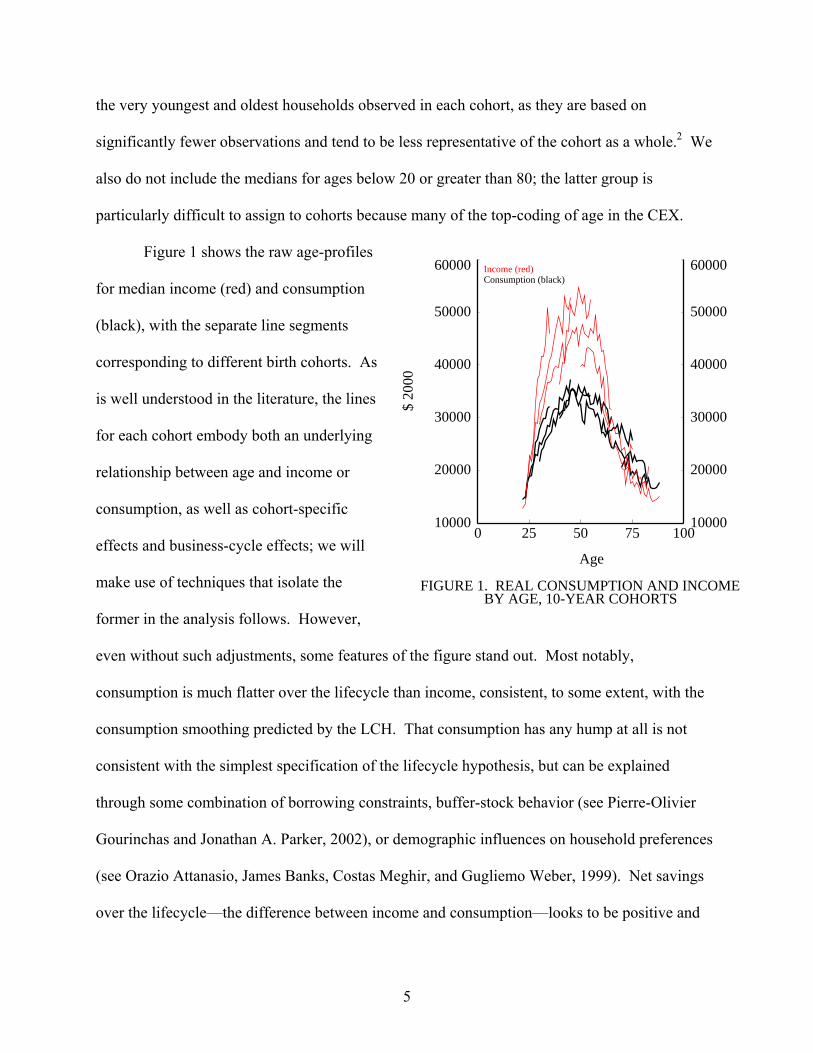
Figure 1 shows the raw age-profiles
for median income (red) and consumption
(black), with the separate line segments
corresponding to different birth cohorts. As
is well understood in the literature, the lines
for each cohort embody both an underlying
relationship between age and income or
consumption, as well as cohort-specific
effects and business-cycle effects; we will
make use of techniques that isolate the
former in the analysis follows. However,
even without such adjustments, some features of the figure stand out. Most notably,
consumption is much flatter over the lifecycle than income, consistent, to some extent, with the
consumption smoothing predicted by the LCH. That consumption has any hump at all is not
consistent with the simplest specification of the lifecycle hypothesis, but can be explained
through some combination of borrowing constraints, buffer-stock behavior (see Pierre-Olivier
Gourinchas and Jonathan A. Parker, 2002), or demographic influences on household preferences
(see Orazio Attanasio, James Banks, Costas Meghir, and Gugliemo Weber, 1999). Net savings
over the lifecycle—the difference between income and consumption—looks to be positive and
0 25 50 75 10010000
20000
30000
40000
50000
60000
10000
20000
30000
40000
50000
60000Income (red)Consumption (black)
FIGURE 1. REAL CONSUMPTION AND INCOMEBY AGE, 10-YEAR COHORTS
$ 20
00
Age

6
quite larger in magnitude than one would expect given the saving rates reported in the NIPA.
We do not view this result as reflecting true behavior so much as a tendency for CEX
respondents to be worse at remembering all of their expenditures than at recalling the full extent
of their income. In any event, we make adjustments to reflect the discrepancy when we draw
lessons for the NIPA saving rate from our CEX results.
III. Using the CEX to Account for Demographic Effects on the Aggregate Saving Rate
The aggregate U.S. saving rate has shown a pronounced downtrend over the past two
decades, falling from an average of 9.1 percent in the 1980s, to 5.2 percent in the 1990s, to
1.6 percent in the first six years of the current decade. We will explore whether the aging of the
population has contributed to this downtrend and how it should be expected to affect aggregate
saving going forward, should current projections of the age structure turn out to be accurate.
The key challenge in using synthetic cohort data to estimate the effect of population
aging on the aggregate saving rate is distinguishing between the various determinants of the
saving of any given cohort at a particular age. In addition to the lifecycle influences on saving
discussed in section I, one would expect saving to vary with the business cycle, as households
seek to smooth their consumption in the face of job losses or other transitory shocks to income.
One might also expect different cohorts to save more or less over the lifecycle, depending, for
example, on differing tastes, shocks to wealth, or changes in social programs providing income
in retirement.
We build on a framework suggested by Orazio Attanasio (1998) for distinguishing
between these factors. We regress median cohort saving rates at each age on a 5th degree
polynomial in age, cohort dummies, and year dummies. The year dummies are included to
capture business-cycle effects; if left unrestricted, however, the coefficients will not be identified
7
because year can be expressed as a linear function of age and cohort. To achieve identification,
we follow Attanasio in restricting the coefficients to average to zero and to be orthogonal to a
linear trend. These identifying assumptions are strong—they imply that all linear trends in the
data are attributable to age or cohort effects. One might be particularly worried that the
estimated cohort effects might pick up business cycle effects if the sample covered just a short
time span that was unbalanced in terms of the phase of the macroeconomic expansion or
contraction. However, this possibility is not a significant obstacle to our analysis since our
primary interest is in the estimated relationship between age and saving.
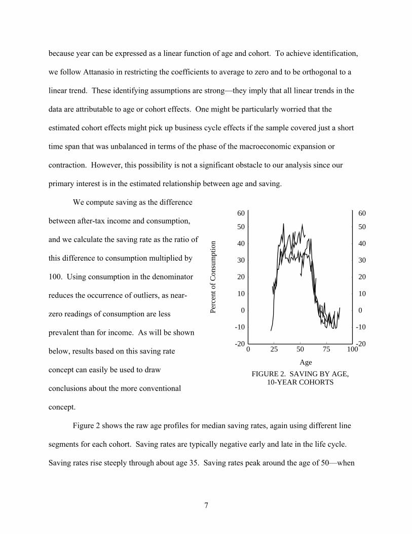
We compute saving as the difference
between after-tax income and consumption,
and we calculate the saving rate as the ratio of
this difference to consumption multiplied by
100. Using consumption in the denominator
reduces the occurrence of outliers, as near-
zero readings of consumption are less
prevalent than for income. As will be shown
below, results based on this saving rate
concept can easily be used to draw
conclusions about the more conventional
concept.
Figure 2 shows the raw age profiles for median saving rates, again using different line
segments for each cohort. Saving rates are typically negative early and late in the life cycle.
Saving rates rise steeply through about age 35. Saving rates peak around the age of 50—when
0 25 50 75 100-20
-10
0
10
20
30
40
50
60
-20
-10
0
10
20
30
40
50
60
FIGURE 2. SAVING BY AGE,10-YEAR COHORTS
Perc
ent o
f Con
sum
ptio
n
Age
8
household income is at its highest—although differences in typical saving rates between about
ages 35 and 55 are rather small. The saving rates also take on some very high values, both
because we put consumption (not income) in the denominator and, we think more important,
because of the aforementioned tendency for CEX households to underreport their consumption
more than their income.
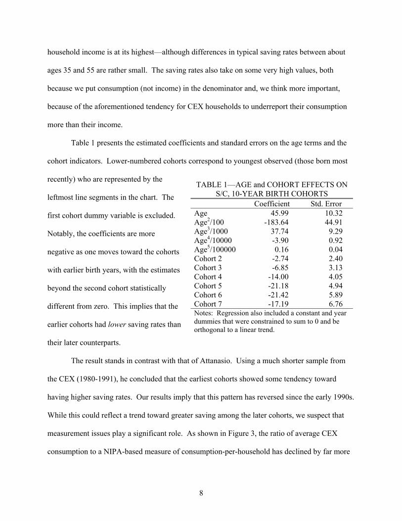
Table 1 presents the estimated coefficients and standard errors on the age terms and the
cohort indicators. Lower-numbered cohorts correspond to youngest observed (those born most
recently) who are represented by the
leftmost line segments in the chart. The
first cohort dummy variable is excluded.
Notably, the coefficients are more
negative as one moves toward the cohorts
with earlier birth years, with the estimates
beyond the second cohort statistically
different from zero. This implies that the
earlier cohorts had lower saving rates than
their later counterparts.
The result stands in contrast with that of Attanasio. Using a much shorter sample from
the CEX (1980-1991), he concluded that the earliest cohorts showed some tendency toward
having higher saving rates. Our results imply that this pattern has reversed since the early 1990s.
While this could reflect a trend toward greater saving among the later cohorts, we suspect that
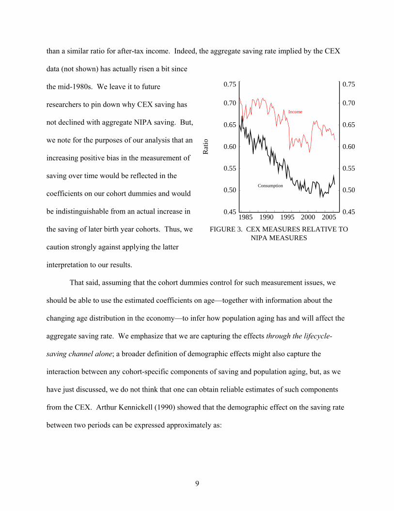
measurement issues play a significant role. As shown in Figure 3, the ratio of average CEX
consumption to a NIPA-based measure of consumption-per-household has declined by far more
TABLE 1—AGE and COHORT EFFECTS ON S/C, 10-YEAR BIRTH COHORTS
Coefficient Std. Error Age 45.99 10.32 Age2/100 -183.64 44.91 Age3/1000 37.74 9.29 Age4/10000 -3.90 0.92 Age5/100000 0.16 0.04 Cohort 2 -2.74 2.40 Cohort 3 -6.85 3.13 Cohort 4 -14.00 4.05 Cohort 5 -21.18 4.94 Cohort 6 -21.42 5.89 Cohort 7 -17.19 6.76 Notes: Regression also included a constant and year dummies that were constrained to sum to 0 and be orthogonal to a linear trend.
9
than a similar ratio for after-tax income. Indeed, the aggregate saving rate implied by the CEX
data (not shown) has actually risen a bit since
the mid-1980s. We leave it to future
researchers to pin down why CEX saving has
not declined with aggregate NIPA saving. But,
we note for the purposes of our analysis that an
increasing positive bias in the measurement of
saving over time would be reflected in the
coefficients on our cohort dummies and would
be indistinguishable from an actual increase in
the saving of later birth year cohorts. Thus, we
caution strongly against applying the latter
interpretation to our results.
That said, assuming that the cohort dummies control for such measurement issues, we
should be able to use the estimated coefficients on age—together with information about the
changing age distribution in the economy—to infer how population aging has and will affect the
aggregate saving rate. We emphasize that we are capturing the effects through the lifecycle-
saving channel alone; a broader definition of demographic effects might also capture the
interaction between any cohort-specific components of saving and population aging, but, as we
have just discussed, we do not think that one can obtain reliable estimates of such components
from the CEX. Arthur Kennickell (1990) showed that the demographic effect on the saving rate
between two periods can be expressed approximately as:
1985 1990 1995 2000 20050.45
0.50
0.55
0.60
0.65
0.70
0.75
0.45
0.50
0.55
0.60
0.65
0.70
0.75
Consumption
Income
FIGURE 3. CEX MEASURES RELATIVE TONIPA MEASURES
Rat
io
10
00
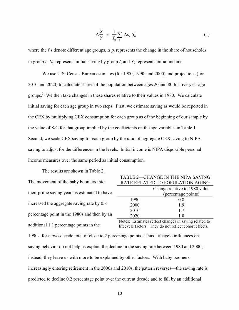
1 ii
i
S p SY Y
Δ ≈ Δ∑ (1)
where the i’s denote different age groups, Δ pi represents the change in the share of households
in group i, 0iS represents initial saving by group I, and Y0 represents initial income.
We use U.S. Census Bureau estimates (for 1980, 1990, and 2000) and projections (for
2010 and 2020) to calculate shares of the population between ages 20 and 80 for five-year age
groups.3 We then take changes in these shares relative to their values in 1980. We calculate
initial saving for each age group in two steps. First, we estimate saving as would be reported in
the CEX by multiplying CEX consumption for each group as of the beginning of our sample by
the value of S/C for that group implied by the coefficients on the age variables in Table 1.
Second, we scale CEX saving for each group by the ratio of aggregate CEX saving to NIPA
saving to adjust for the differences in the levels. Initial income is NIPA disposable personal
income measures over the same period as initial consumption.
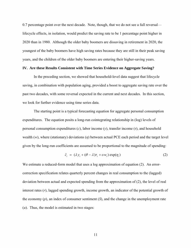
The results are shown in Table 2.
The movement of the baby boomers into
their prime saving years is estimated to have
increased the aggregate saving rate by 0.8
percentage point in the 1980s and then by an
additional 1.1 percentage points in the
1990s, for a two-decade total of close to 2 percentage points. Thus, lifecycle influences on
saving behavior do not help us explain the decline in the saving rate between 1980 and 2000;
instead, they leave us with more to be explained by other factors. With baby boomers
increasingly entering retirement in the 2000s and 2010s, the pattern reverses—the saving rate is
predicted to decline 0.2 percentage point over the current decade and to fall by an additional
TABLE 2—CHANGE IN THE NIPA SAVING RATE RELATED TO POPULATION AGING
Change relative to 1980 value (percentage points)
1990 0.8 2000 1.9 2010 1.7 2020 1.0
Notes: Estimates reflect changes in saving related to lifecycle factors. They do not reflect cohort effects.
11
0.7 percentage point over the next decade. Note, though, that we do not see a full reversal—
lifecycle effects, in isolation, would predict the saving rate to be 1 percentage point higher in
2020 than in 1980. Although the older baby boomers are dissaving in retirement in 2020, the
youngest of the baby boomers have high saving rates because they are still in their peak saving
years, and the children of the older baby boomers are entering their higher-saving years.
IV. Are these Results Consistent with Time Series Evidence on Aggregate Saving?
In the preceding section, we showed that household-level data suggest that lifecycle
saving, in combination with population aging, provided a boost to aggregate saving rate over the
past two decades, with some reversal expected in the current and next decades. In this section,
we look for further evidence using time series data.
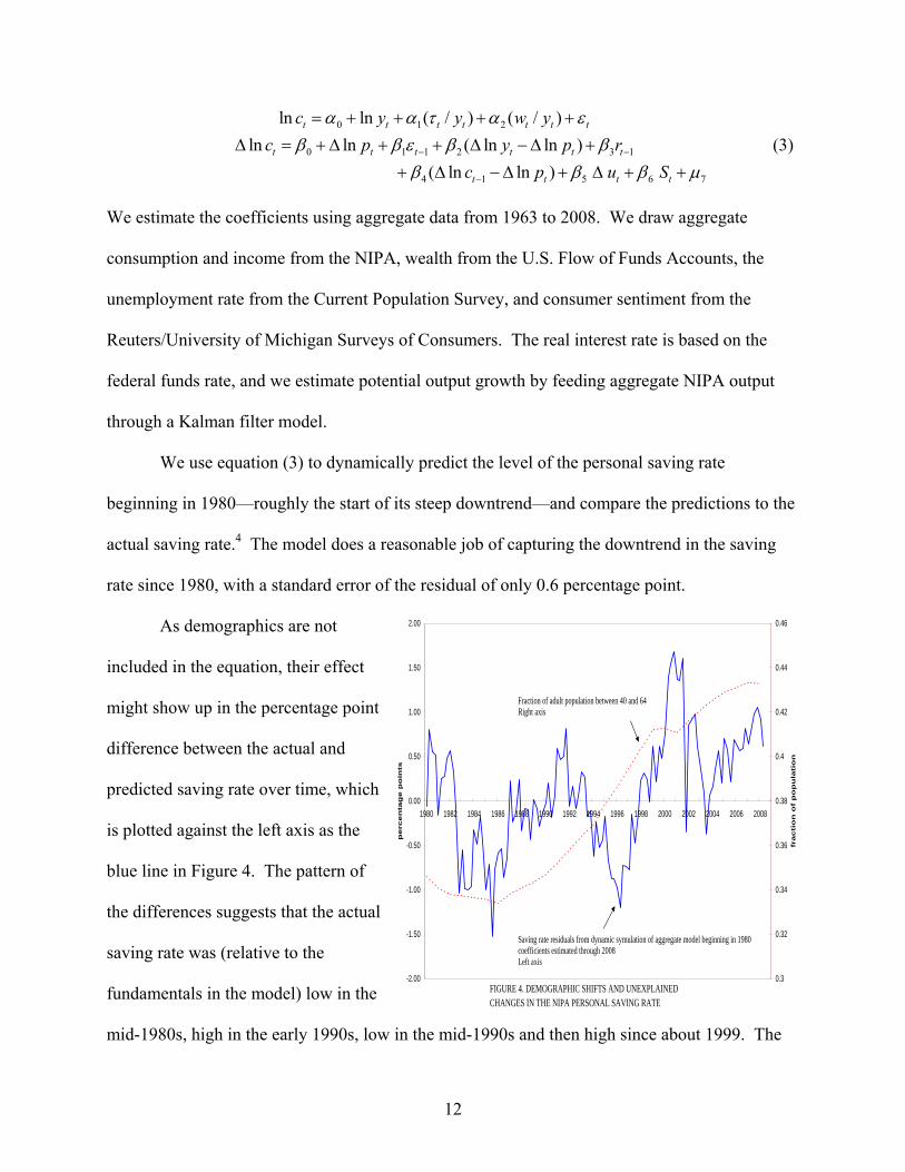
The starting point is a typical forecasting equation for aggregate personal consumption
expenditures. The equation posits a long-run cointegrating relationship in (log) levels of
personal consumption expenditures (c), labor income (y), transfer income (τ), and household
wealth (w), where (stationary) deviations (η) between actual PCE each period and the target level
given by the long-run coefficients are assumed to be proportional to the magnitude of spending:
( ( ) ) exp( )t t t t tc y wλ θ λ τ υ η= + − + (2)
We estimate a reduced-form model that uses a log approximation of equation (2). An error-
correction specification relates quarterly percent changes in real consumption to the (lagged)
deviation between actual and expected spending from the approximation of (2), the level of real
interest rates (r), lagged spending growth, income growth, an indicator of the potential growth of
the economy (p), an index of consumer sentiment (S), and the change in the unemployment rate
(u). Thus, the model is estimated in two stages:
12
0 1 2
0 1 1 2 3 1
4 1 5 6 7
ln ln ( / ) ( / )ln ln ( ln ln )
( ln ln )
t t t t t t t
t t t t t t
t t t t
c y y w yc p y p r
c p u S
α α τ α εβ β ε β β
β β β μ− −
−
= + + + +Δ = + Δ + + Δ −Δ +
+ Δ −Δ + Δ + + (3)
We estimate the coefficients using aggregate data from 1963 to 2008. We draw aggregate
consumption and income from the NIPA, wealth from the U.S. Flow of Funds Accounts, the
unemployment rate from the Current Population Survey, and consumer sentiment from the
Reuters/University of Michigan Surveys of Consumers. The real interest rate is based on the
federal funds rate, and we estimate potential output growth by feeding aggregate NIPA output
through a Kalman filter model.
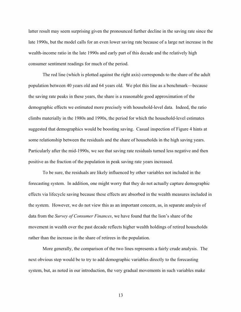
We use equation (3) to dynamically predict the level of the personal saving rate
beginning in 1980—roughly the start of its steep downtrend—and compare the predictions to the
actual saving rate.4 The model does a reasonable job of capturing the downtrend in the saving
rate since 1980, with a standard error of the residual of only 0.6 percentage point.
As demographics are not
included in the equation, their effect
might show up in the percentage point
difference between the actual and
predicted saving rate over time, which
is plotted against the left axis as the
blue line in Figure 4. The pattern of
the differences suggests that the actual
saving rate was (relative to the
fundamentals in the model) low in the
mid-1980s, high in the early 1990s, low in the mid-1990s and then high since about 1999. The
-2.00
-1.50
-1.00
-0.50
0.00
0.50
1.00
1.50
2.00
1980 1982 1984 1986 1988 1990 1992 1994 1996 1998 2000 2002 2004 2006 2008
perc
en
tag
e p
oin
ts
0.3
0.32
0.34
0.36
0.38
0.4
0.42
0.44
0.46
fracti
on
of
po
pu
lati
on
Fraction of adult population between 40 and 64Right axis
Saving rate residuals from dynamic symulation of aggregate model beginning in 1980coefficients estimated through 2008Left axis
FIGURE 4. DEMOGRAPHIC SHIFTS AND UNEXPLAINED CHANGES IN THE NIPA PERSONAL SAVING RATE
13
latter result may seem surprising given the pronounced further decline in the saving rate since the
late 1990s, but the model calls for an even lower saving rate because of a large net increase in the
wealth-income ratio in the late 1990s and early part of this decade and the relatively high
consumer sentiment readings for much of the period.
The red line (which is plotted against the right axis) corresponds to the share of the adult
population between 40 years old and 64 years old. We plot this line as a benchmark—because
the saving rate peaks in these years, the share is a reasonable good approximation of the
demographic effects we estimated more precisely with household-level data. Indeed, the ratio
climbs materially in the 1980s and 1990s, the period for which the household-level estimates
suggested that demographics would be boosting saving. Casual inspection of Figure 4 hints at
some relationship between the residuals and the share of households in the high saving years.
Particularly after the mid-1990s, we see that saving rate residuals turned less negative and then
positive as the fraction of the population in peak saving rate years increased.
To be sure, the residuals are likely influenced by other variables not included in the
forecasting system. In addition, one might worry that they do not actually capture demographic
effects via lifecycle saving because these effects are absorbed in the wealth measures included in
the system. However, we do not view this as an important concern, as, in separate analysis of
data from the Survey of Consumer Finances, we have found that the lion’s share of the
movement in wealth over the past decade reflects higher wealth holdings of retired households
rather than the increase in the share of retirees in the population.
More generally, the comparison of the two lines represents a fairly crude analysis. The
next obvious step would be to try to add demographic variables directly to the forecasting
system, but, as noted in our introduction, the very gradual movements in such variables make

14
identification difficult, particularly if factors such as tastes and the economic environment facing
the household are also changing gradually.
V. Aging and the Relationship between Changes in Consumption and Income
We can use the CEX data to compare the relative magnitudes of typical changes in
consumption from age to age with typical changes in income to get a handle on how closely they
tend to move together. Algebraically, the ratio of the age-differentials for consumption, dcda
, and
income, dyda
, defines a differential of consumption to income, dcdy
. However, interpreting that
ratio is not straightforward. With respect to income, we capture typical changes over the
lifecycle—very different in nature from the sort of “shock” that is often considered when
estimating the mpc. Moreover, the correspondence observed between lifecycle changes in
consumption and income may not even be causal. That said, we think it is informative to use our
comprehensive CEX data to revisit how closely consumption tracks income over the lifecycle, in
the spirit, for instance, of Christopher D. Carroll and Lawrence H. Summers (1991).
We estimate dcda
and dyda
with separate regressions. To preserve the nonlinear age-
consumption and age-income profiles apparent in the raw CEX cohort data, we use linear spline
regression models with knots that correspond to the 12 five-year age groups between ages 20 and
80. Using household-level data (restricted as above), we regress real consumption (and then real
income) on the spline terms, as well as cohort and time dummies, with the latter restricted as in
our saving rate regressions. Our procedure estimates the typical change in consumption (or in
income) as households age; within a five-year age group, the relationship is linear, but the slope
is allowed to vary non-linearly as households move across age categories.
15
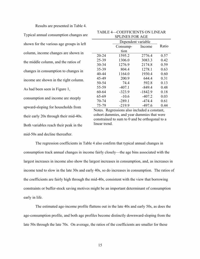
Results are presented in Table 4.
Typical annual consumption changes are
shown for the various age groups in left
column, income changes are shown in
the middle column, and the ratios of
changes in consumption to changes in
income are shown in the right column.
As had been seen in Figure 1,
consumption and income are steeply
upward-sloping for households from
their early 20s through their mid-40s.
Both variables reach their peak in the
mid-50s and decline thereafter.
The regression coefficients in Table 4 also confirm that typical annual changes in
consumption track annual changes in income fairly closely—the age bins associated with the
largest increases in income also show the largest increases in consumption, and, as increases in
income tend to slow in the late 30s and early 40s, so do increases in consumption. The ratios of
the coefficients are fairly high through the mid-40s, consistent with the view that borrowing
constraints or buffer-stock saving motives might be an important determinant of consumption
early in life.
The estimated age-income profile flattens out in the late 40s and early 50s, as does the
age-consumption profile, and both age profiles become distinctly downward-sloping from the
late 50s through the late 70s. On average, the ratios of the coefficients are smaller for these
TABLE 4—COEFFICIENTS ON LINEAR SPLINES FOR AGE
Dependent variable Consump-
tion Income Ratio
20-24 1595.2 2776.4 0.57 25-39 1306.0 3083.3 0.42 30-34 1276.9 2174.8 0.59 35-39 804.4 1278.1 0.63 40-44 1164.0 1930.4 0.60 45-49 200.9 644.4 0.31 50-54 74.4 592.8 0.13 55-59 -407.1 -849.4 0.48 60-64 -323.9 -1842.9 0.18 65-69 -10.6 -407.2 0.03 70-74 -289.1 -474.4 0.61 75-79 -219.9 -497.6 0.44
Notes. Regressions also included a constant, cohort dummies, and year dummies that were constrained to sum to 0 and be orthogonal to a linear trend.
16
groups than for the younger groups. One interpretation of the change would be that households’
incomes have risen sufficiently such that borrowing constraints no longer bind by this age or that
households have already built their desired precautionary buffers. Given our concerns about the
interpretation of the dcdy
implied by lifecycle patterns of consumption and income in household
data, we do not attempt to formally tie our estimates to the aggregate mpc as we did for the
saving rate. However, the analysis is at least suggestive that the aggregate marginal propensity
to consume might have been expected to decline as the baby boomers moved out of its early
working years and into the years in which their spending patterns were not dominated by
borrowing constraints or precautionary motives.
VI. Using Time Series Data to Estimate Demographic Effects on the Aggregate Marginal
Propensity to Consume out of Disposable Personal Income
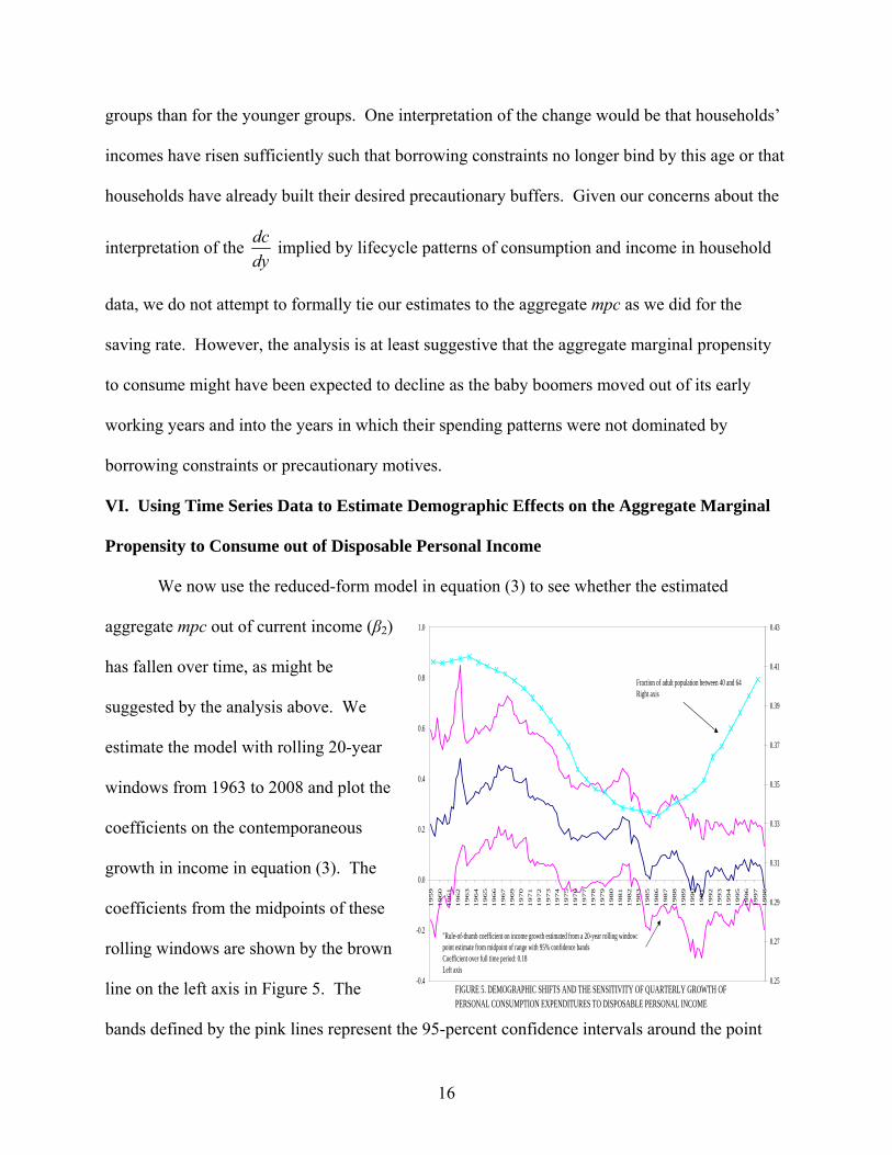
We now use the reduced-form model in equation (3) to see whether the estimated
aggregate mpc out of current income (β2)
has fallen over time, as might be
suggested by the analysis above. We
estimate the model with rolling 20-year
windows from 1963 to 2008 and plot the
coefficients on the contemporaneous
growth in income in equation (3). The
coefficients from the midpoints of these
rolling windows are shown by the brown
line on the left axis in Figure 5. The
bands defined by the pink lines represent the 95-percent confidence intervals around the point
-0.4
-0.2
0.0
0.2
0.4
0.6
0.8
1.0
1959
1960
1961
1962
1963
1964
1965
1966
1967
1969
1970
1971
1972
1973
1974
1975
1976
1977
1978
1979
1980
1981
1982
1983
1985
1986
1987
1988
1989
1990
1991
1992
1993
1994
1995
1996
1997
1998
0.25
0.27
0.29
0.31
0.33
0.35
0.37
0.39
0.41
0.43
"Rule-of-thumb coefficient on income growth estimated from a 20-year rolling window:point estimate from midpoint of range with 95% confidence bandsCoefficient over full time period: 0.18Left axis
Fraction of adult population between 40 and 64Right axis
FIGURE 5. DEMOGRAPHIC SHIFTS AND THE SENSITIVITY OF QUARTERLY GROWTH OFPERSONAL CONSUMPTION EXPENDITURES TO DISPOSABLE PERSONAL INCOME

17
estimates. As can be seen, the point estimates fall over the period shown. In fact, they are not
statistically different from 0 after the mid-1980s.
There are different ways in which this parameter can be interpreted. John Y. Campbell
and N. Gregory Mankiw (1990) interpret the coefficient on contemporaneous aggregate income
from a similar framework as the fraction of the population represented by so-called “rule-of-
thumb” households who spend their current income instead of smoothing consumption according
to the LCH. One might also interpret this coefficient as the fraction of any given household’s
consumption that is matched one-for-one with income changes—in other words, an mpc out of
current income.
Again, as a benchmark, we show the fraction of the adult population between ages 40 and
64 (the dashed line plotted against the right axis). After 1980 or so, the mpc declines as the
portion of the population in peak saving years increases. However, the share of the population in
this group is also high in the 1960s and early 1970s, a period when the estimated aggregate mpc
is much larger and statistically significant. Thus, the evidence for a significant demographic
effect on the aggregate mpc is, at best, weak. Indeed, other factors are at play; for example,
Karen E. Dynan, Douglas W. Elmendorf, and Daniel E. Sichel (2006) interpret the lower mpc
observed since the early 1980s as reflecting a greater ability to smooth consumption because of
financial innovation.
VII. Conclusion
Analysis based on household-level data suggests that population aging has had a material
effect on the pattern of the aggregate saving rate over time. In particular, the movement of the
baby boom into its higher saving years should have provided an increasing boost to the aggregate
saving rate in the 1980s and 1990s. We expect some reversal of this pattern as this cohort moves

18
into retirement in the current and next decade. Furthermore, we show with time series data, that
these effects appear to be at least roughly consistent with the realized pattern of the aggregate
saving rate, after controlling for other determinants. Our analysis regarding the aggregate
marginal propensity to consume comes to less firm conclusions. The household-level data are, at
best, suggestive that demographics might explain why time series data exhibit a reduced
response of consumption to contemporaneous income over the past two decades.
19
REFERENCES
Attanasio, Orazio. 1998. “A Cohort Analysis of Saving Behaviour by U.S. Households.”
Journal of Human Resources, 33(3): 575-609.
Attanasio, Orazio, James W. Banks, Costas Meghir, and Gugliemo Weber. “Humps and Bumps
in Lifetime Consumption.” 1999. Journal of Business and Economic Statistics, 17(1):
22-35.
Blinder, Alan S. “Distribution Effects and the Aggregate Consumption Function.” 1975.
Journal of Political Economy, 83( 3): 447-475.
Browning, Martin, Angus Deaton, and Margaret Irish. 1985. “A Profitable Approach to Labor
Supply and Commodity Demands over the Life-Cycle.” Econometrica, 53(3): 503-543.
Campbell, John Y., and N. Gregory Mankiw. 1990. “Permanent Income, Current Income, and
Consumption,” Journal of Business and Economic Statistics 8(3), 265-79.
Carroll, Christopher D., and Lawrence H. Summers. 1991. “Consumption Growth Parallels
Income Growth: Some New Evidence.” In National Saving and Economic Performance,
ed. B. Douglas Bernheim and John B. Shoven, 305-48. Chicago: University of Chicago
Press.
Dominguez, Kathryn M., and Ray C. Fair. 1991. “Effects of the Changing U.S. Age
Distribution on Macroeconomic Equations.” American Economic Review, 81(5): 1276-
94.
Dynan, Karen E., Douglas W. Elmendorf, and Daniel E. Sichel. 2006. “Can Financial
Innovation Help to Explain the Reduced Volatility of Economic Activity?” Journal of
Monetary Economics, 53(1): 123-50.

20
Gourinchas, Pierre-Olivier and Jonathan A. Parker. 2002. “Consumption Over the Life Cycle.”
Econometrica, 70(1): 47-89.
Kennickell, Arthur. 1990. “Demographics and Household Savings.” Federal Reserve Board
Finance and Economics Discussion Series Number 123.

21
* Dynan: Federal Reserve Board, Washington, DC 20551 (email: [email protected]); Edelberg: Federal Reserve Board, Washington, DC 20551 (email: [email protected]); Palumbo: Federal Reserve Board, Washington, DC 20551 (email: [email protected]). We thank … for helpful comments. The views expressed are those of the authors and not necessarily those of the Federal Reserve Board or the other members of its staff.
1 An appendix with a more complete description of the data is available upon request from the authors. 2 For example, the medians for the 46-year-olds for the cohort born between 1960 and 1969 are based solely on data for households born in 1960 or the first quarter of 1961 and interviewed in 2006 or the first quarter of 2007. 3 Data limitations prevent us from doing the calculation precisely. For example, ideally, we would like to use shares of households with heads of different ages rather than shares of the population at different ages. However, the estimates presented are not very sensitive to modest changes in the underlying data, so we believe they are informative about the sign and the rough magnitude of the actual effects. 4 This simulation fixes all coefficients at the values estimated for the full sample and then conditions on actual realizations of the determinants of consumption.
Recommended