The effects of climate on the epidemiology of plague in
Madagascar Kathy Kreppel
Matthew Baylis; Sandra Telfer; Lila Rahalison; Andy Morse

Presently 38 countries in Asia, Africa and America report human plague cases
Most cases annually reported from the African continent
Within the African countries 60% of all cases reported from Madagascar and
Tanzania
Human Plague
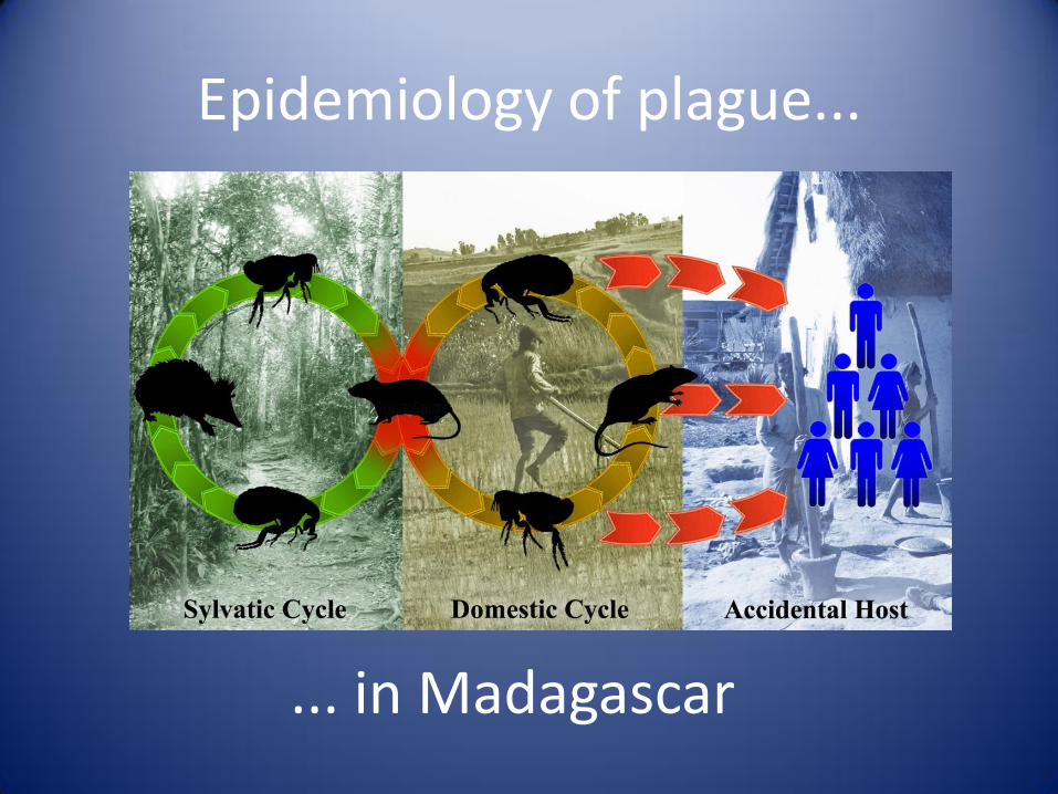
Epidemiology of plague...
... in Madagascar

Climate
Humidity • Precipitation • Temperature
Flea vector density Flea vector infection rate
Rodent host parasite burden
Proportion of infected rodents
Flea vector habitat
&
Pathogen environment
Micro-Climate
Desiccation • Flooding • Temperature Fluctuation
Pathogen within vector
• Pathogen survival • Pathogen multiplication
Flea Vector
• Reproduction rate • Development rate • Adult longevity

16
17
18
19
20
21
22
23
24
25
0 10 20 30 40 50 60 70 80 90
Jan
Feb
Mar
Ap
r M
ay Ju
n
Jul
Au
g Sep
O
ct N
ov
Dec
Cas
es
Average monthly plague cases and average monthly temperature °C
Tem
per
atu
re
C°
Wet and Hot
Wet and Hot
Dry and Cool
Climate and plague Climate effects on plague are not obvious and direct as with malaria
Copyright: Jamstec
Madagascar is affected by:
- El Niño Southern Oscillation (ENSO)
- Indian Ocean Dipole (IOD)
- Frequent cyclones

Climate analysis El Niño event => drier and warmer conditions than usual 12 months later
(the hot season gets hotter)
Positive IOD => warmer conditions than usual 1-2 months later (the cold
season gets warmer)
Significant correlations in time frequency
space
- ENSO and plague
- IOD and plague
El Nino => decreased plague incidence
9-12 months later
Positive IOD => increased plague
incidence 1-2 months later
Interplay can result in plague epidemics

ENSO and plague incidence
Figure: Phase angle evolution of JMA and incidence anomalies with 2-5 year periodicity. The
red line represents incidence anomalies, the blue line the ENSO index. The x-axis is the
wavelet location in time. The y-axis denotes the phase angles.

Summary of climate analysis
Global climate:
- El Niño Southern Oscillation affects human
plague in Madagscar
- The Indian Ocean Dipole affects plague
incidence from the 1990s
-There is a non-stationarity in the
relationship

Districts reporting
plague from 1975 to
2008
1. Absence – Presence
Maximum Entropy model
2. Magnitude of incidence
Linear regression model
Spatial analysis of plague incidence and
environmental variables
MODIS variables:
-NDVI
-EVI
-MIR
-dLST
-nLST
Altitude

Maximum Entropy
Response curve of the NDVI to plague presence Response curve of dLST to plague presence
Model performance Response curve of altitude to plague presence

Absence – Presence
Altitude is positively correlated with
plague presence in districts
NDVI is negatively correlated (peak
timing of triannual cycle)
dLST is positively correlated (peak
timing of biannual cycle and
variation )
nLST is positively correlated (peak
timing of biannual cycle)
Magnitude of incidence
nLST is negatively correlated
dLST is negatively correlated
EVI is positively correlated
MIR (amplitude) is positively
correlated
Spatial analysis of plague incidence and environmental variables

Effects on....
Vector
- mortality
- survival
- development
Rodent Host
- Mortality
- survival
- Habitat
Pathogen
- Temperature
Human host
- migration
- poverty
- crop choice
- housing conditions

Study location
Step 1

Micro-climate
9
11
13
15
17
19
21
23
25
Jan Apr Jul Sep Nov
Tem
pe
ratu
re *
C
Average burrow temperatures
House burrow temperature
Outside burrow temperature
• It is warmer and less humid indoors • Temperature values are very similar between house burrows and outside burrows • Humidity values show large differences
70
75
80
85
90
95
100
Jan Apr Jul Sep Nov
Re
lati
ve H
um
idit
y %
Average burrow humidities
House burrow humidity
Outside burrow humidity

0
0.2
0.4
0.6
0.8
1
1.2
1.4
1.6
1.8
2
Jan-0
9
Ap
r-09
Jul-0
9
Sep-0
9
No
v-09
Feb-1
0
Fle
a in
dex
Fieldtrip
Number of fleas per trapped rat
Xch
Sf
Sf is more abundant in the cold months July and September, while Xch is most abundant in November... is the endemic Sf adapted to the colder highlands?
Fleas

Laboratory data • Larvae of the endemic Sf pupate on average 8.5 days later
• At individual temperatures humidity affects development
• No consistent effect of humidity across the range of temperatures
• Humidity seems to affect Sf more
0
5
10
15
20
25
30
35
40
18 21 25 28.5 32
Me
an d
eve
lop
me
nt
tim
e in
day
s
Temperature ˚C
Mean development time of Sf at different treatments
At 80%RH
At 90% RH
0
5
10
15
20
25
30
35
40
18 21 25 28.5 32
Me
an d
eve
lop
me
nt
tim
e in
day
s
Temperature ˚C
Mean development time of Xch at different treatments
At 80% RH
At 90% RH
Endemic Sf Ubiquitous Xch
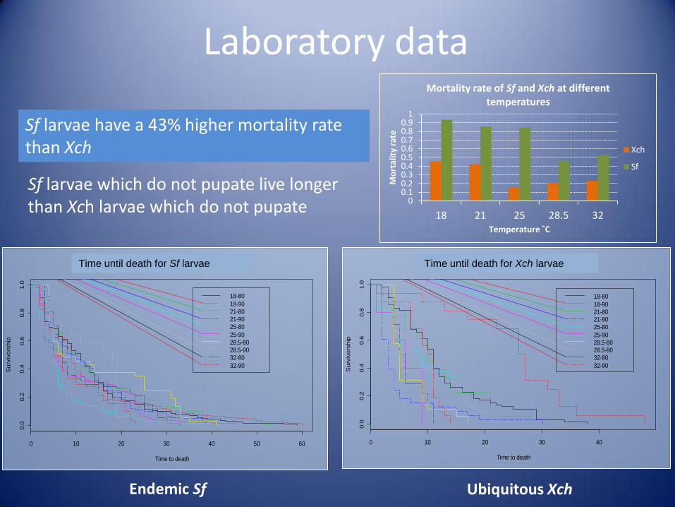
Laboratory data
Sf larvae have a 43% higher mortality rate than Xch
0 0.1 0.2 0.3 0.4 0.5 0.6 0.7 0.8 0.9
1
18 21 25 28.5 32
Mo
rtal
ity
rate
Temperature ˚C
Mortality rate of Sf and Xch at different temperatures
Xch
Sf
Endemic Sf Ubiquitous Xch
0 10 20 30 40 50 60
0.0
0.2
0.4
0.6
0.8
1.0
Time to death
Su
rviv
ors
hip
Time to death for Sf. by treatment
18-80
18-90
21-80
21-90
25-80
25-90
28.5-80
28.5-90
32-80
32-90
0 10 20 30 40
0.0
0.2
0.4
0.6
0.8
1.0
Time to death
Su
rviv
ors
hip
Time to death of Xch per treatment
18-80
18-90
21-80
21-90
25-80
25-90
28.5-80
28.5-90
32-80
32-90
Time until death for Sf larvae Time until death for Xch larvae
Sf larvae which do not pupate live longer than Xch larvae which do not pupate

Combining field and laboratory data
0 5
10 15 20 25 30 35 40 45 50 55 60 65 70 75
Jan Apr Jul Sep Dec
Days to complete larval development in an outside burrow
Xch outside
Sf outside
0 5
10 15 20 25 30 35 40 45 50 55 60 65 70 75
Jan Apr Jul Sep Dec
Days to complete larval development in a house burrow
Xch inside
Sf inside
The larvae of Sf take longer to develop than Xch except in an outside burrow during July

Summary of vector study
Vector presence all year round Vectors link the exterior focus with houses – human infection Sf have a slight advantage in summer
Xenopsylla
cheopis
(ubiquitous)
Synopsyllus
fonquerniei
(endemic)

Conclusion
- Temperature and humidity affect the vectors Plague season onset
-All year round vector cover and transmission
cycle is only in the highlands Altitudinal threshold
-Host burrow climate differs between indoor
and outdoor Different habitats favoured at different times of the year

Overall conclusions • Climate does affect human plague incidence in Madagascar
Global climate drivers such as El Niño and the Indian Ocean Dipole influence the epidemiology of plague
• Spatial analysis identified altitude and environmental variables such as vegetation cover and temperature as predictors of presence and absence of plague and magnitude of incidence
• Evidence suggests that temperature and humidity
have a significant effect on both flea vectors
• This implies that climate and environmental variables have an impact and could be used as warning and forecasting tools in a country with very limited resources.

Acknowledgements
I would like to thank my supervisors
Sandra Telfer, Matthew Baylis and Andy Morse for help and support, Nohal Elissa for the opportunity to work in Entomology at the IPM, and LUCINDA
group members for moral support!
Many thanks to the technicians Corinne and Tojo for their help with the lab experiment and the
technicians of the plague unit for their hard work during each field trip.

Questions?

Environmental variables
Variable Feature Coefficient
Average altitude quadratic
hinge
9.016
-0.319
Average NDVI peak
timing of triannual cycle
quadratic -1.082
Average dLST peak
timing of biannual cycle
linear 0.668
Average dLSTd2 quadratic 0.937
Average nLSTp2 quadratic 0.875

Magnitude of plague Variable Feature Coefficient Std Error t P>|t| 95% Conf. Interval
Average MIR a2 linear -.0717949 .0194965 -3.68 0.001 -.1114164 -.0321733
Average MIR a2 quadratic .0001889 .0000496 3.81 0.001 .0000881 .0002896
Average MIR d2 linear .3156656 .121508 2.60 0.014 .0687316 .5625995
Average dLST d2 linear .3680068 .086814 4.24 0.000 .1915796 .544434
Average dLST d2 quadratic -.0074938 .0019328 -3.88 0.000 -.0114217 -.0035658
Average nLST d1 linear .1554398 .0291623 5.33 0.000 .0961749 .2147047
Average nLST d1 quadratic -.001523 .0003071 -4.96 0.000 -.0021472 -.0008989
Average EVI d3 linear -1.919053 .5244084 -3.66 0.001 -2.984779 -.8533271
Average EVI d3 quadratic .7311711 .2387242 3.06 0.004 .2460252 1.216317
Constant -3.123993 .9695764 -3.22 0.003 -5.094409 -1.153577
Recommended