The Divergence of Stock Index
Futures from Their Underlying
Cash Values*
J.Q. Hu
Fudan University
August 24, 2017

Introduction
Stock Index Futures was first introduced in US in
1982 (SP500 futures)
Since then, stock index futures have been
introduced in many markets in different countries,
and CSI 300 index futures was introduced in
China in 2010.
In general, stock index futures prices are based on
the cost-to-carry model (Cornell and France 1983)
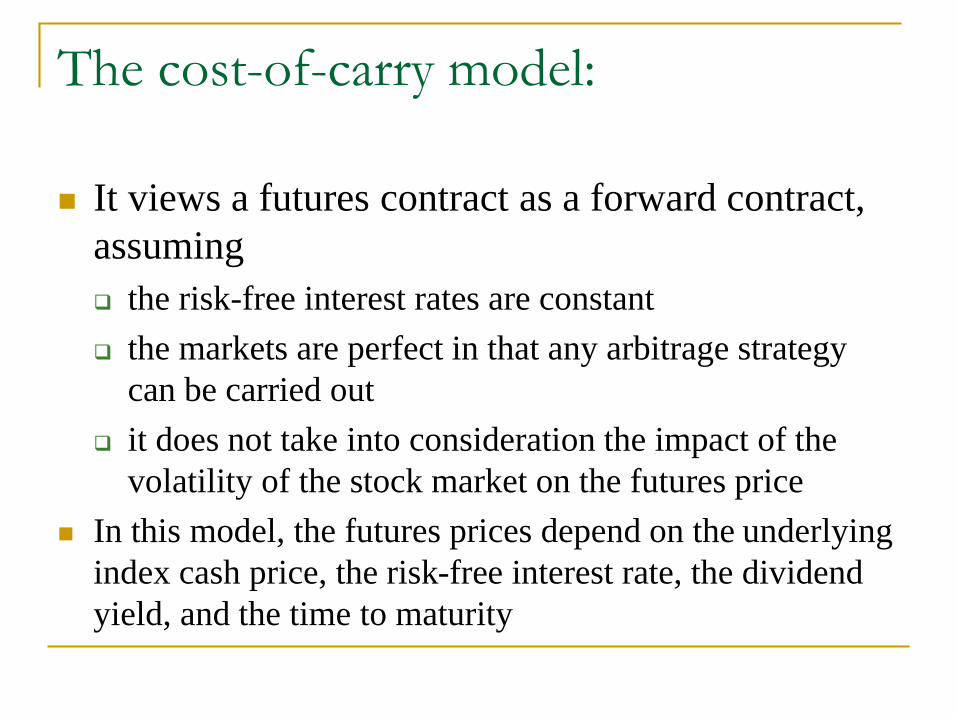
The cost-of-carry model:
It views a futures contract as a forward contract,
assuming
the risk-free interest rates are constant
the markets are perfect in that any arbitrage strategy
can be carried out
it does not take into consideration the impact of the
volatility of the stock market on the futures price
In this model, the futures prices depend on the underlying
index cash price, the risk-free interest rate, the dividend
yield, and the time to maturity

Introduction
No-arbitrage model with stochastic interest rates
(Ranaswamy and Sundaresan 1985)
Models in which both interest rates and market
volatility are stochastic (Bailey and Stulz 1989,
Hemler and Longstaff 1991)
However, very few study on the effects of trading
and regulatory constraints on index futures prices.

The basis of CSI 300 stock indexbasis = futures price – cash price

The basic model(based on the work by Robert Jarrow (1980), “Heterogeneous Expectations, Restrictions on Short
Sales, and Equilibrium Asset Prices.” The Journal of Finance.)
Consider a market with 𝐾 investors, J risky assets,
and one risk-free asset
▪ Investor 𝑘 ∈ {1,… , 𝐾}
▪ Asset 𝑗 ∈ {0,1,… , J}, (0 is risk-free asset)
The basic model
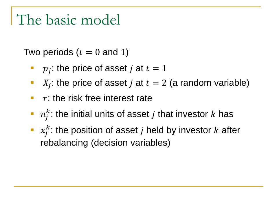
Two periods (𝑡 = 0 and 1)
▪ 𝑝𝑗: the price of asset 𝑗 at 𝑡 = 1
▪ 𝑋𝑗: the price of asset 𝑗 at 𝑡 = 2 (a random variable)
▪ 𝑟: the risk free interest rate
▪ 𝑛𝑗𝑘: the initial units of asset 𝑗 that investor 𝑘 has
▪ 𝑥𝑗𝑘: the position of asset 𝑗 held by investor 𝑘 after
rebalancing (decision variables)
The basic model
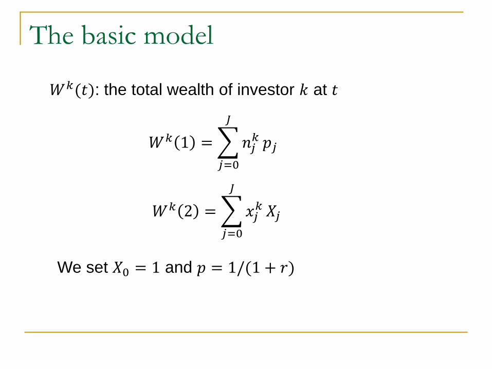
𝑊𝑘(𝑡): the total wealth of investor 𝑘 at 𝑡
𝑊𝑘 1 =
𝑗=0
𝐽
𝑛𝑗𝑘 𝑝𝑗
𝑊𝑘 2 =
𝑗=0
𝐽
𝑥𝑗𝑘 𝑋𝑗
We set 𝑋0 = 1 and 𝑝 = 1/(1 + 𝑟)

The basic model
For investor 𝑘, his utility is given by
𝑈𝑘 𝑊𝑘 2 = 𝐸𝑘 𝑊𝑘 2 − 𝛼𝑘𝑉𝑎𝑟𝑘[𝑊𝑘 2 ]
where 𝛼𝑘 > 0 is a constant measuring risk aversion,
and 𝐸𝑘[∙] and 𝑉𝑎𝑟𝑘[∙] are the expectation and
variance taken w.r.t the distribution of investor 𝑘’s
belief regarding asset payoffs.
The basic model
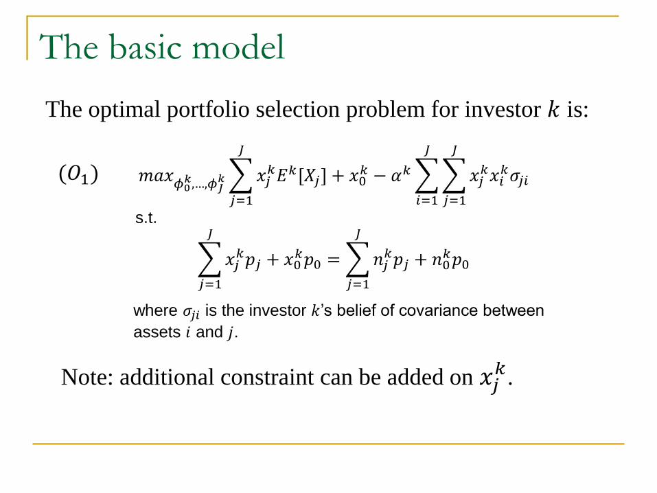
The optimal portfolio selection problem for investor 𝑘 is:
𝑚𝑎𝑥𝜙0𝑘,…,𝜙𝐽
𝑘
𝑗=1
𝐽
𝑥𝑗𝑘𝐸𝑘[𝑋𝑗] + 𝑥0
𝑘 − 𝛼𝑘
𝑖=1
𝐽
𝑗=1
𝐽
𝑥𝑗𝑘𝑥𝑖
𝑘𝜎𝑗𝑖
s.t.
𝑗=1
𝐽
𝑥𝑗𝑘𝑝𝑗 + 𝑥0
𝑘𝑝0 =
𝑗=1
𝐽
𝑛𝑗𝑘𝑝𝑗 + 𝑛0
𝑘𝑝0
(𝑂1)
where 𝜎𝑗𝑖 is the investor 𝑘’s belief of covariance between
assets 𝑖 and 𝑗.
Note: additional constraint can be added on 𝑥𝑗𝑘.

Equilibrium
Definition: A vector 𝑃∗ ∈ 𝑅𝐽 is called an
equilibrium price of the market if there exist 𝑥𝑘∗ ∈𝑅𝐽 for 𝑘 = 1,⋯ ,𝐾 such that
𝑥𝑘∗ solves the optimization problem 𝑂1 at 𝑃 = 𝑃∗ for
𝑘 = 1,⋯ , 𝐾
σ𝑘=1𝐾 𝑥𝑘∗ = σ𝑘=1
𝐾 𝑁𝑘 for 𝑗 = 1,⋯ , 𝐽.
where 𝑁𝑘 = 𝑛1𝑘 , ⋯ , 𝑛𝐽
𝐾 𝑇
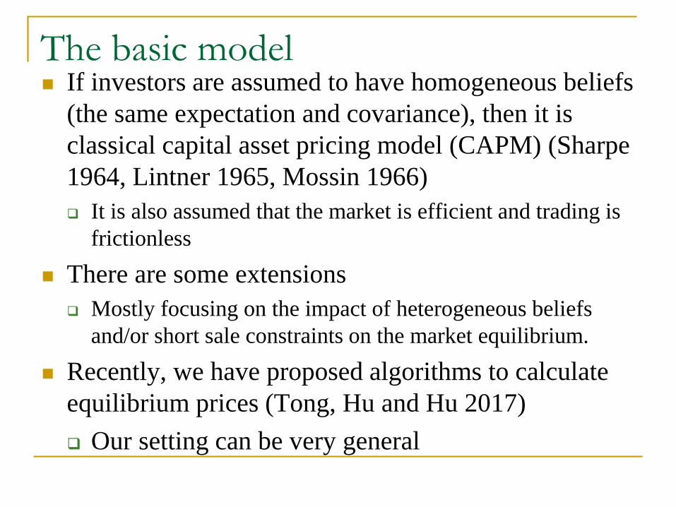
The basic model If investors are assumed to have homogeneous beliefs
(the same expectation and covariance), then it is
classical capital asset pricing model (CAPM) (Sharpe
1964, Lintner 1965, Mossin 1966)
It is also assumed that the market is efficient and trading is
frictionless
There are some extensions
Mostly focusing on the impact of heterogeneous beliefs
and/or short sale constraints on the market equilibrium.
Recently, we have proposed algorithms to calculate
equilibrium prices (Tong, Hu and Hu 2017)
Our setting can be very general

Model (with stock index futures)
Investor 𝑘 ∈ 1,…𝐾
Asset 𝑗 ∈ 0,1,… 𝐽 (0 is the risk-free asset)
𝜔𝑗 is the weight of asset j in the stock index (j=1,…,J)
Consider a market with 𝐾 investors, one risk-free
asset (bond), J risky assets (stocks), and stock index
futures
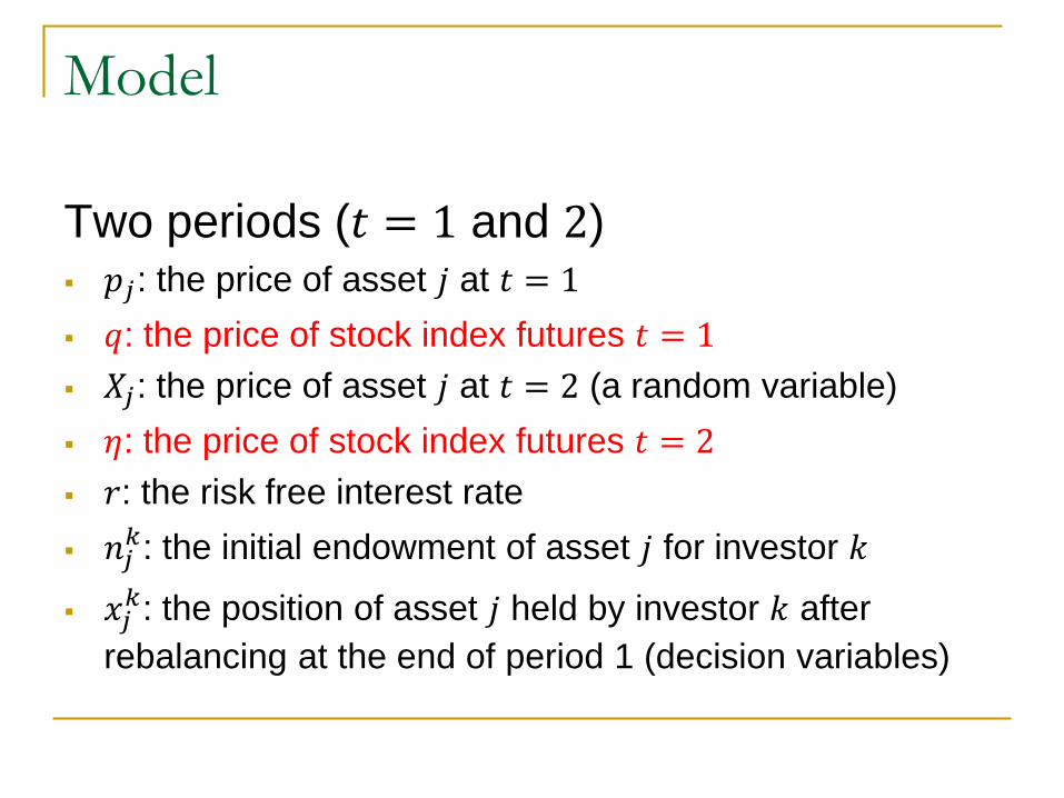
Model
Two periods (𝑡 = 1 and 2)▪ 𝑝𝑗: the price of asset 𝑗 at 𝑡 = 1
▪ 𝑞: the price of stock index futures 𝑡 = 1
▪ 𝑋𝑗: the price of asset 𝑗 at 𝑡 = 2 (a random variable)
▪ 𝜂: the price of stock index futures 𝑡 = 2
▪ 𝑟: the risk free interest rate
▪ 𝑛𝑗𝑘: the initial endowment of asset 𝑗 for investor 𝑘
▪ 𝑥𝑗𝑘: the position of asset 𝑗 held by investor 𝑘 after
rebalancing at the end of period 1 (decision variables)
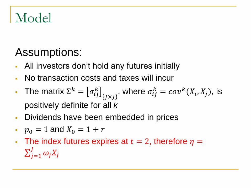
Model
Assumptions:▪ All investors don’t hold any futures initially
▪ No transaction costs and taxes will incur
▪ The matrix Σ𝑘 = 𝜎𝑖𝑗𝑘
𝐽×𝐽, where 𝜎𝑖𝑗
𝑘 = 𝑐𝑜𝑣𝑘(𝑋𝑖 , 𝑋𝑗), is
positively definite for all k
▪ Dividends have been embedded in prices
▪ 𝑝0 = 1 and 𝑋0 = 1 + 𝑟
▪ The index futures expires at 𝑡 = 2, therefore 𝜂 =
σ𝑗=1𝐽
𝜔𝑗𝑋𝑗

The model
𝑊𝑘(𝑡): the total wealth of investor 𝑘 at 𝑡, we have
𝑊𝑘 1 = 𝑛0𝑘 +
𝑗=1
𝐽
𝑛𝑗𝑘 𝑝𝑗 = 𝑥0
𝑘 +
𝑗=1
𝐽
𝑥𝑗𝑘 𝑝𝑗 + 𝑞𝑓𝑘
𝑊𝑘 2 = 1 + 𝑟 𝑥0𝑘 + σ𝑗=1
𝐽𝑥𝑗𝑘 𝑋𝑗 + 𝜂𝑓𝑘
= 𝑊𝑘 1 + 𝑋 − 𝑃 𝑇𝑥𝑘 + 𝜔𝑇𝑋 − 𝑞 𝑓𝑘 + 𝑟𝑥0𝑘
𝑤ℎ𝑒𝑟𝑒 𝑋 = 𝑋1, … , 𝑋𝐽𝑇, 𝑃 = 𝑝1, … , 𝑝𝐽
𝑇,
𝜔 = 𝜔1, … , 𝜔𝐽 , 𝑥𝑘 = (𝑥1𝑘 , … , 𝑥𝐽
𝑘)

Model
For investor 𝑘, his utility is given by
𝑈𝑘 𝑊𝑘 2 = 𝐸𝑘 𝑊𝑘 2 − 𝛼𝑘𝑉𝑎𝑟𝑘[𝑊𝑘 2 ]
where 𝛼𝑘 > 0 is a constant measuring risk aversion, and
𝐸𝑘[∙] and 𝑉𝑎𝑟𝑘[∙] are the expectation and variance taken
w.r.t the distribution of investor 𝑘’s belief regarding asset
payoffs.
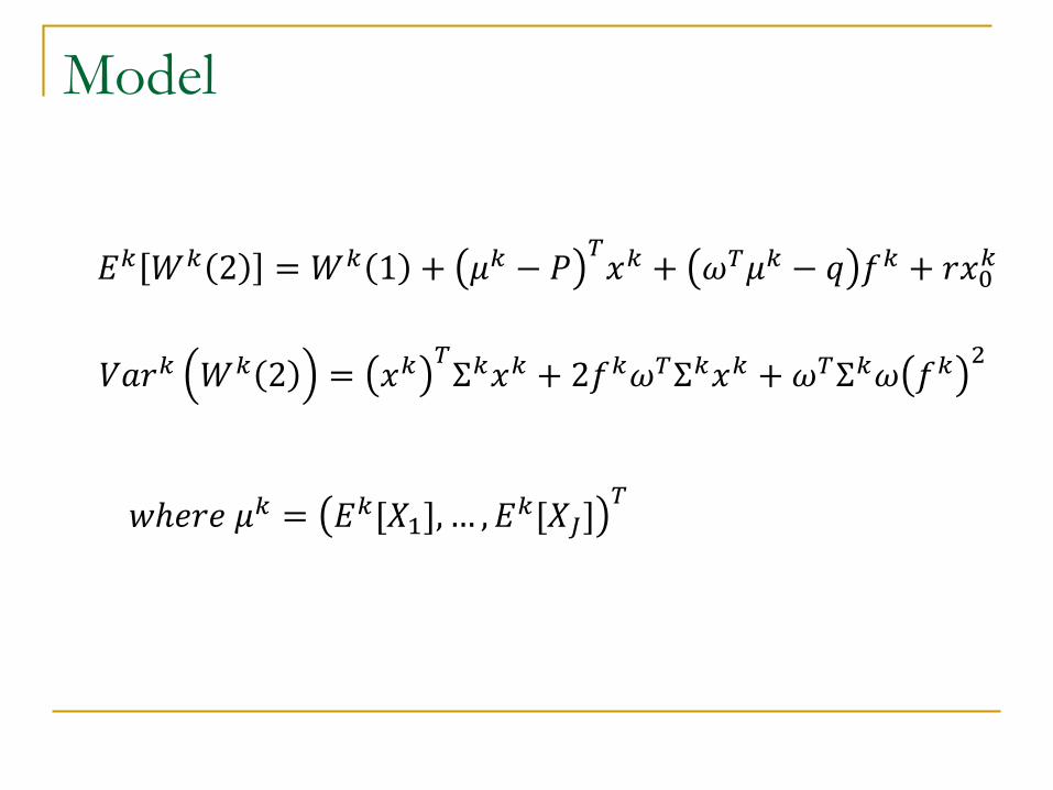
Model
𝐸𝑘 𝑊𝑘 2 = 𝑊𝑘 1 + 𝜇𝑘 − 𝑃𝑇𝑥𝑘 + 𝜔𝑇𝜇𝑘 − 𝑞 𝑓𝑘 + 𝑟𝑥0
𝑘
𝑉𝑎𝑟𝑘 𝑊𝑘 2 = 𝑥𝑘𝑇Σ𝑘𝑥𝑘 + 2𝑓𝑘𝜔𝑇Σ𝑘𝑥𝑘 +𝜔𝑇Σ𝑘𝜔 𝑓𝑘
2
𝑤ℎ𝑒𝑟𝑒 𝜇𝑘 = 𝐸𝑘[𝑋1], … , 𝐸𝑘[𝑋𝐽]𝑇

The basic problem
In a perfect market (with no trading restriction), the
optimal portfolio selection problem for investor 𝑘 is:
𝑚𝑎𝑥𝑥0𝑘,…,𝑥𝐽
𝑘,𝑓𝑘𝑈𝑘 𝑊𝑘 2
s.t. 𝑃𝑇𝑥𝑘 + 𝑞𝑓𝑘 + 𝑥0𝑘 = 𝑃𝑇𝑁𝑘 + 𝑁0
𝑘
(𝑃𝑀𝑘)
Note: additional constraint can be added on 𝑥𝑗𝑘 later.
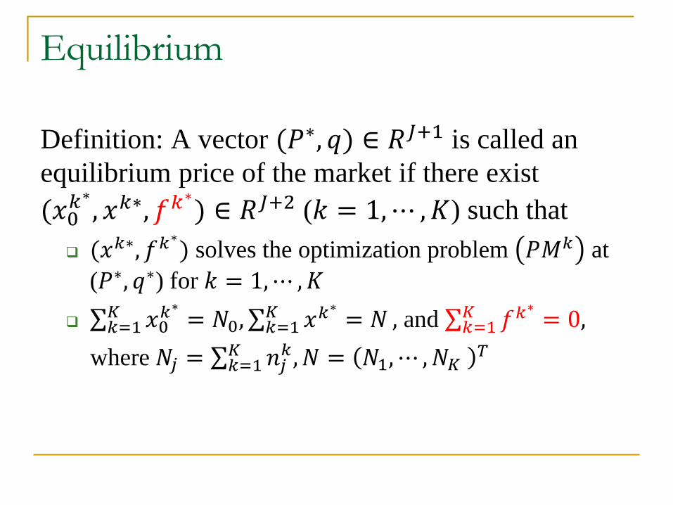
Equilibrium
Definition: A vector (𝑃∗, 𝑞) ∈ 𝑅𝐽+1 is called an
equilibrium price of the market if there exist
(𝑥0𝑘∗ , 𝑥𝑘∗, 𝑓𝑘
∗) ∈ 𝑅𝐽+2 (𝑘 = 1,⋯ ,𝐾) such that
(𝑥𝑘∗, 𝑓𝑘∗) solves the optimization problem 𝑃𝑀𝑘 at
(𝑃∗, 𝑞∗) for 𝑘 = 1,⋯ , 𝐾
σ𝑘=1𝐾 𝑥0
𝑘∗ = 𝑁0, σ𝑘=1𝐾 𝑥𝑘
∗= 𝑁 , and σ𝑘=1
𝐾 𝑓𝑘∗= 0,
where 𝑁𝑗 = σ𝑘=1𝐾 𝑛𝑗
𝑘 , 𝑁 = 𝑁1, ⋯ , 𝑁𝐾𝑇

Main Results
𝐸𝑘 𝑊𝑘 2 = 𝑊𝑘 1 + 𝜇𝑘 − 𝑃𝑇𝑥𝑘 + 𝜔𝑇𝜇𝑘 − 𝑞 𝑓𝑘 + 𝑟𝑥0
𝑘
𝑉𝑎𝑟𝑘 𝑊𝑘 2 = 𝑥𝑘𝑇Σ𝑘𝑥𝑘 + 2𝑓𝑘𝜔𝑇Σ𝑘𝑥𝑘 +𝜔𝑇Σ𝑘𝜔 𝑓𝑘
2
𝑚𝑎𝑥𝑥0𝑘,…,𝑥𝐽
𝑘,𝑓𝑘𝐸𝑘 𝑊𝑘 2 − 𝛼𝑘𝑉𝑎𝑟𝑘[𝑊𝑘 2 ]
s.t. 𝑃𝑇𝑥𝑘 + 𝑞𝑓𝑘 + 𝑥0𝑘 = 𝑃𝑇𝑁𝑘 + 𝑁0
𝑘
(𝑃𝑀𝑘)
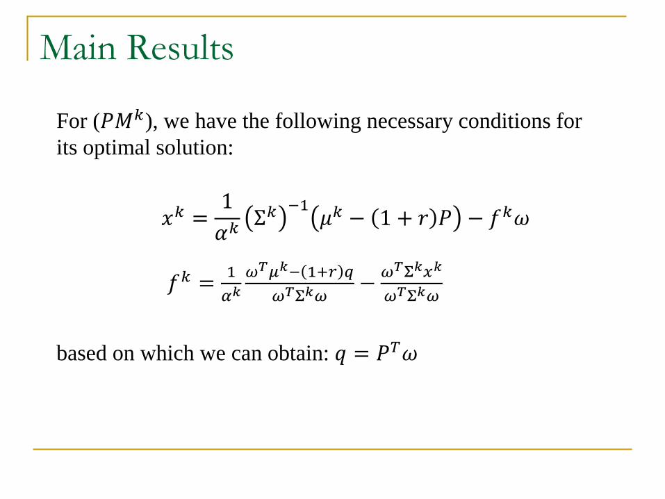
Main Results
𝑥𝑘 =1
𝛼𝑘Σ𝑘
−1𝜇𝑘 − 1 + 𝑟 𝑃 − 𝑓𝑘𝜔
𝑓𝑘 =1
𝛼𝑘𝜔𝑇𝜇𝑘− 1+𝑟 𝑞
𝜔𝑇Σ𝑘𝜔−
𝜔𝑇Σ𝑘𝑥𝑘
𝜔𝑇Σ𝑘𝜔
For (𝑃𝑀𝑘), we have the following necessary conditions for
its optimal solution:
based on which we can obtain: 𝑞 = 𝑃𝑇𝜔
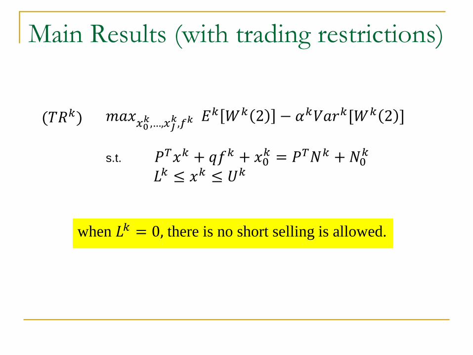
Main Results (with trading restrictions)
𝑚𝑎𝑥𝑥0𝑘,…,𝑥𝐽
𝑘,𝑓𝑘𝐸𝑘 𝑊𝑘 2 − 𝛼𝑘𝑉𝑎𝑟𝑘[𝑊𝑘 2 ]
s.t. 𝑃𝑇𝑥𝑘 + 𝑞𝑓𝑘 + 𝑥0𝑘 = 𝑃𝑇𝑁𝑘 + 𝑁0
𝑘
𝐿𝑘 ≤ 𝑥𝑘 ≤ 𝑈𝑘
(𝑇𝑅𝑘)
when 𝐿𝑘 = 0, there is no short selling is allowed.
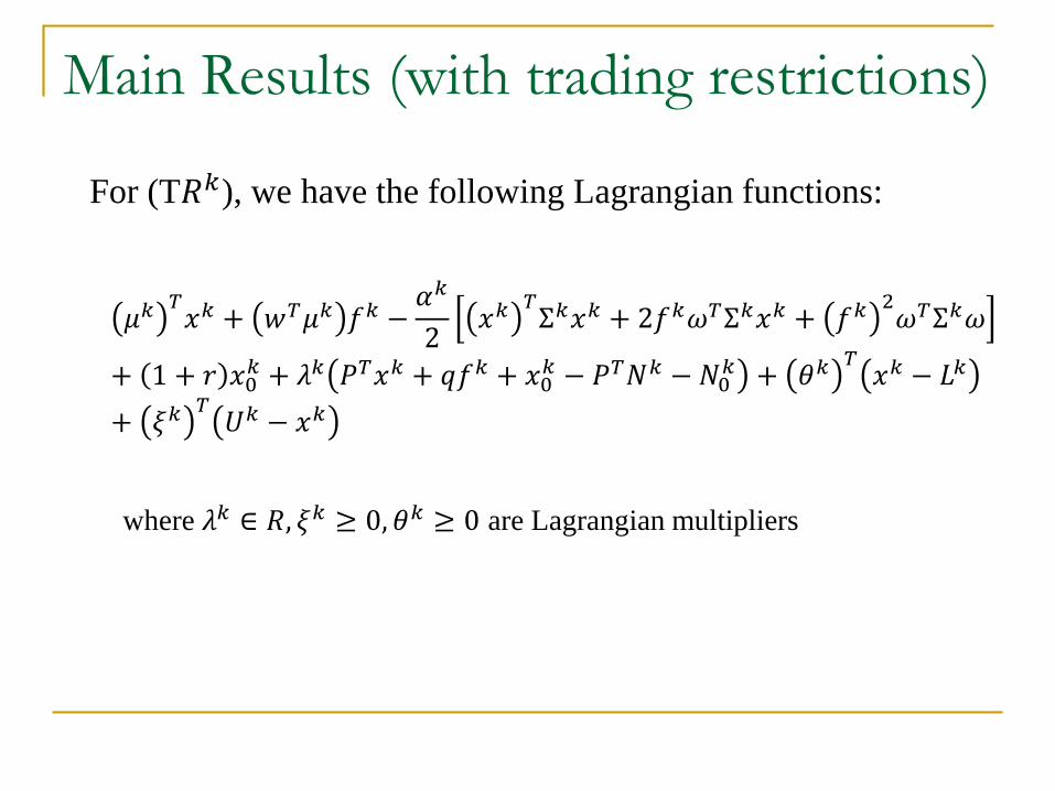
Main Results (with trading restrictions)
𝜇𝑘𝑇𝑥𝑘 + 𝑤𝑇𝜇𝑘 𝑓𝑘 −
𝛼𝑘
2𝑥𝑘
𝑇Σ𝑘𝑥𝑘 + 2𝑓𝑘𝜔𝑇Σ𝑘𝑥𝑘 + 𝑓𝑘
2𝜔𝑇Σ𝑘𝜔
+ 1 + 𝑟 𝑥0𝑘 + 𝜆𝑘 𝑃𝑇𝑥𝑘 + 𝑞𝑓𝑘 + 𝑥0
𝑘 − 𝑃𝑇𝑁𝑘 − 𝑁0𝑘 + 𝜃𝑘
𝑇𝑥𝑘 − 𝐿𝑘
+ 𝜉𝑘𝑇𝑈𝑘 − 𝑥𝑘
where 𝜆𝑘 ∈ 𝑅, 𝜉𝑘 ≥ 0, 𝜃𝑘 ≥ 0 are Lagrangian multipliers
For (T𝑅𝑘), we have the following Lagrangian functions:
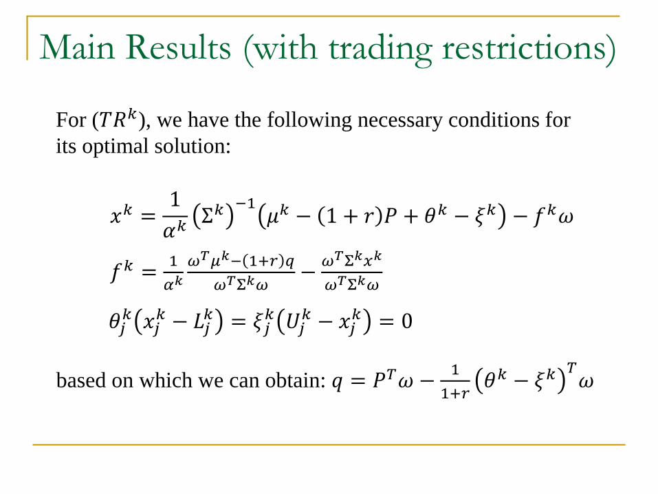
Main Results (with trading restrictions)
𝑥𝑘 =1
𝛼𝑘Σ𝑘
−1𝜇𝑘 − 1 + 𝑟 𝑃 + 𝜃𝑘 − 𝜉𝑘 − 𝑓𝑘𝜔
𝑓𝑘 =1
𝛼𝑘𝜔𝑇𝜇𝑘− 1+𝑟 𝑞
𝜔𝑇Σ𝑘𝜔−
𝜔𝑇Σ𝑘𝑥𝑘
𝜔𝑇Σ𝑘𝜔
For (𝑇𝑅𝑘), we have the following necessary conditions for
its optimal solution:
𝜃𝑗𝑘 𝑥𝑗
𝑘 − 𝐿𝑗𝑘 = 𝜉𝑗
𝑘 𝑈𝑗𝑘 − 𝑥𝑗
𝑘 = 0
based on which we can obtain: 𝑞 = 𝑃𝑇𝜔 −1
1+𝑟𝜃𝑘 − 𝜉𝑘
𝑇𝜔

Main Results (with trading restrictions)
Hence, in general, we have 𝑞 ≠ 𝑃𝑇𝜔.
In particular, if 𝑈𝑘 = ∞, then 𝜉𝑘 = 0, we have 𝑞 ≤ 𝑃𝑇𝜔

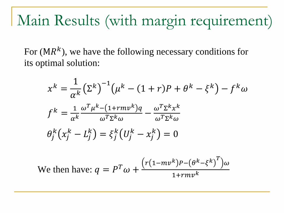
Main Results (with margin requirement)
𝑚𝑎𝑥𝑥0𝑘,…,𝑥𝐽
𝑘,𝑓𝑘𝐸𝑘 𝑊𝑘 2 − 𝛼𝑘𝑉𝑎𝑟𝑘[𝑊𝑘 2 ]
s.t. 𝑃𝑇𝑥𝑘 +𝑚𝑞 𝑓𝑘 + 𝑥0𝑘 = 𝑃𝑇𝑁𝑘 +𝑁0
𝑘
𝐿𝑘 ≤ 𝑥𝑘 ≤ 𝑈𝑘
(𝑀𝑅𝑘)
where 0 < 𝑚 ≤ 1 is the margin requirement for trading
stock index futures, i.e., if an investor trades (either
longs or shorts) one unit of stock index futures, then his
margin requirement is m units of cash.

Main Results (with margin requirement)
𝜇𝑘 − 𝑃𝑇𝑥𝑘 + 𝑤𝑇𝜇𝑘 − 𝑞 𝑓𝑘
−𝛼𝑘
2𝑥𝑘
𝑇Σ𝑘𝑥𝑘 + 2𝑓𝑘𝜔𝑇Σ𝑘𝑥𝑘 + 𝑓𝑘
2𝜔𝑇Σ𝑘𝜔 + 𝑟𝑥0
𝑘
+ 𝜆𝑘 𝑃𝑇𝑥𝑘 +𝑚𝑞|𝑓𝑘| + 𝑥0𝑘 − 𝑃𝑇𝑁𝑘 − 𝑁0
𝑘 + 𝜃𝑘𝑇𝑥𝑘 − 𝐿𝑘
+ 𝜉𝑘𝑇𝑈𝑘 − 𝑥𝑘
where 𝜆𝑘 ∈ 𝑅, 𝜉𝑘 ≥ 0, 𝜃𝑘 ≥ 0 are Lagrangian multipliers
For (M𝑅𝑘), we have the following Lagrangian functions:
Main Results (with margin requirement)
𝑥𝑘 =1
𝛼𝑘Σ𝑘
−1𝜇𝑘 − 1 + 𝑟 𝑃 + 𝜃𝑘 − 𝜉𝑘 − 𝑓𝑘𝜔
𝑓𝑘 =1
𝛼𝑘𝜔𝑇𝜇𝑘− 1+𝑟𝑚𝑣𝑘 𝑞
𝜔𝑇Σ𝑘𝜔−
𝜔𝑇Σ𝑘𝑥𝑘
𝜔𝑇Σ𝑘𝜔
For (M𝑅𝑘), we have the following necessary conditions for
its optimal solution:
𝜃𝑗𝑘 𝑥𝑗
𝑘 − 𝐿𝑗𝑘 = 𝜉𝑗
𝑘 𝑈𝑗𝑘 − 𝑥𝑗
𝑘 = 0
We then have: 𝑞 = 𝑃𝑇𝜔 +𝑟 1−𝑚𝑣𝑘 𝑃− 𝜃𝑘−𝜉𝑘
𝑇𝜔
1+𝑟𝑚𝑣𝑘
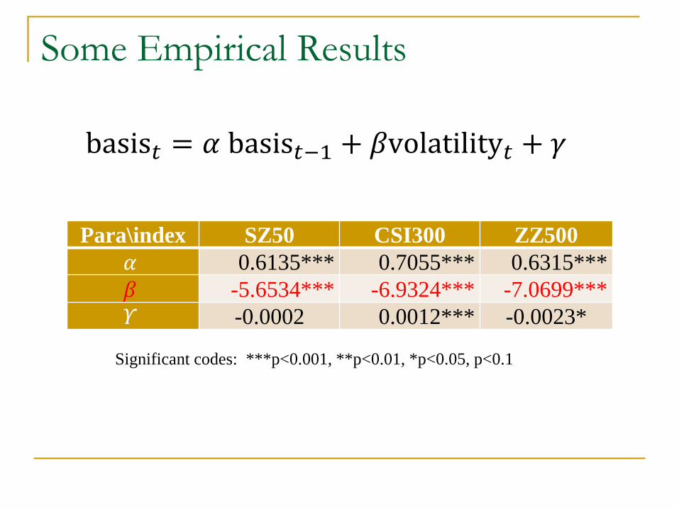
Some Empirical Results
Para\index SZ50 CSI300 ZZ500
𝛼 0.6135*** 0.7055*** 0.6315***
𝛽 -5.6534*** -6.9324*** -7.0699***
𝛶 -0.0002 0.0012*** -0.0023*
basis𝑡 = 𝛼 basis𝑡−1 + 𝛽volatility𝑡 + 𝛾
Significant codes: ***p<0.001, **p<0.01, *p<0.05, p<0.1
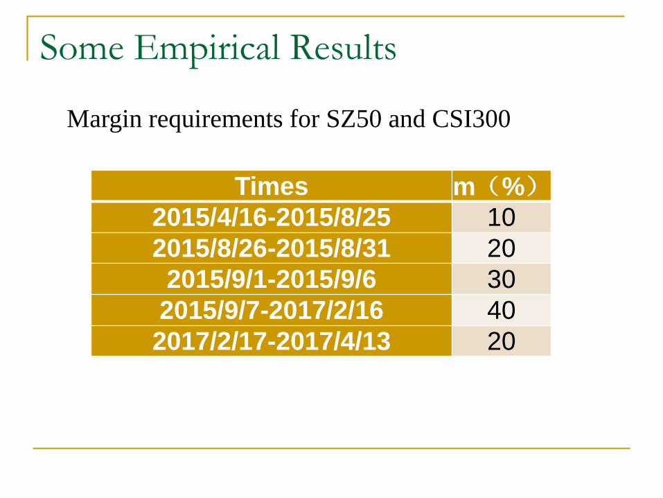
Some Empirical Results
Times m(%)2015/4/16-2015/8/25 10
2015/8/26-2015/8/31 20
2015/9/1-2015/9/6 30
2015/9/7-2017/2/16 40
2017/2/17-2017/4/13 20
Margin requirements for SZ50 and CSI300

Some Empirical Results
basis𝑡 = 𝛼 ∗ basis𝑡−1 + 𝛽 ∗ volatility𝑡 + 𝛾 + 𝑘 ∗ Dummyt
Para\index SZ50 CSI300
𝛼 0.5683*** 0.6031***
𝛽 -8.4435*** -9.8030***
𝛶 0.0034* 0.0016
k -0.0035** -0.0024*
as m increases from 10% to 40% …

Some Empirical Results
basis𝑡 = 𝛼 ∗ basis𝑡−1 + 𝛽 ∗ volatility𝑡 + 𝛾 + 𝑘 ∗ Dummyt
Para\index SZ50 CSI300
𝛼 0.3716*** 0.5098***
𝛽 -5.8229*** -6.6331***
𝛶 -0.0026*** -0.0033***
k 0.0015* 0.0018*
as m decreases from 40% to 20% …

Disclaimer: try this at your own risk …

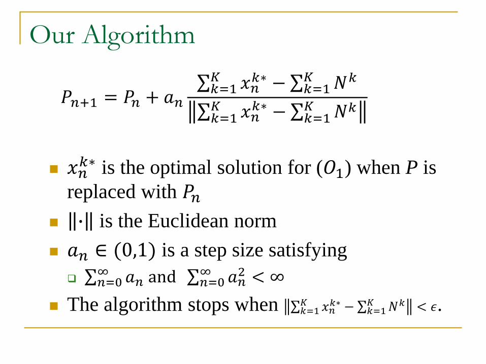
Our Algorithm
𝑥𝑛𝑘∗ is the optimal solution for (𝑂1) when P is
replaced with 𝑃𝑛 ∙ is the Euclidean norm
𝑎𝑛 ∈ (0,1) is a step size satisfying
σ𝑛=0∞ 𝑎𝑛 and σ𝑛=0
∞ 𝑎𝑛2 < ∞
The algorithm stops when σ𝑘=1𝐾 𝑥𝑛
𝑘∗ − σ𝑘=1𝐾 𝑁𝑘 < 𝜖.
𝑃𝑛+1 = 𝑃𝑛 + 𝑎𝑛σ𝑘=1𝐾 𝑥𝑛
𝑘∗ − σ𝑘=1𝐾 𝑁𝑘
σ𝑘=1𝐾 𝑥𝑛
𝑘∗ − σ𝑘=1𝐾 𝑁𝑘
Our Algorithm
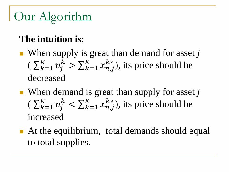
The intuition is:
When supply is great than demand for asset j
( σ𝑘=1𝐾 𝑛𝑗
𝑘 > σ𝑘=1𝐾 𝑥𝑛,𝑗
𝑘∗ ), its price should be
decreased
When demand is great than supply for asset j
( σ𝑘=1𝐾 𝑛𝑗
𝑘 < σ𝑘=1𝐾 𝑥𝑛,𝑗
𝑘∗ ), its price should be
increased
At the equilibrium, total demands should equal
to total supplies.
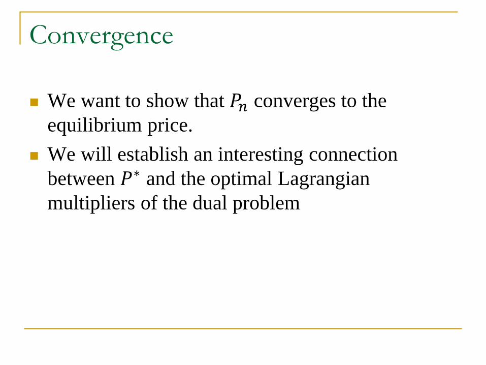
Convergence
We want to show that 𝑃𝑛 converges to the
equilibrium price.
We will establish an interesting connection
between 𝑃∗ and the optimal Lagrangian
multipliers of the dual problem
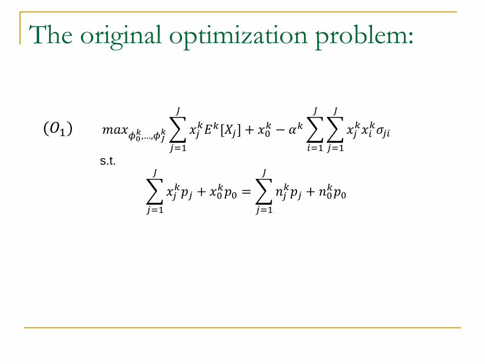
The original optimization problem:
𝑚𝑎𝑥𝜙0𝑘,…,𝜙𝐽
𝑘
𝑗=1
𝐽
𝑥𝑗𝑘𝐸𝑘[𝑋𝑗] + 𝑥0
𝑘 − 𝛼𝑘
𝑖=1
𝐽
𝑗=1
𝐽
𝑥𝑗𝑘𝑥𝑖
𝑘𝜎𝑗𝑖
s.t.
𝑗=1
𝐽
𝑥𝑗𝑘𝑝𝑗 + 𝑥0
𝑘𝑝0 =
𝑗=1
𝐽
𝑛𝑗𝑘𝑝𝑗 + 𝑛0
𝑘𝑝0
(𝑂1)

Convergence
Theorem 1. Assume an equilibrium price 𝑃∗ exists. The
optimization problem (𝑂1) at 𝑃 = 𝑃∗ for 𝑘 = 1,⋯ , 𝐾have the same optimal solutions as the following
problem:
𝑚𝑎𝑥𝜙1𝑘,…,𝜙𝐽
𝑘
𝑘=1
𝐾
𝑗=1
𝐽
𝑥𝑗𝑘𝐸𝑘[𝑋𝑗] − 𝛼𝑘
𝑖=1
𝐽
𝑗=1
𝐽
𝑥𝑗𝑘𝑥𝑖
𝑘𝜎𝑗𝑖
s.t.
𝑘=1
𝐾
𝑥𝑗𝑘 =
𝑘=1
𝐾
𝑛𝑗𝑘 , 𝑗 = 1,⋯ , 𝐽
(𝑂3)

Convergence
(𝑂3) doesn’t depend explicitly on 𝑃∗. So what is
the connection between 𝑃∗ and (𝑂3)?
(𝑂3)𝑚𝑎𝑥𝜙1
𝑘,…,𝜙𝐽𝑘
𝑘=1
𝐾
𝑗=1
𝐽
𝑥𝑗𝑘𝐸𝑘[𝑋𝑗] − 𝛼𝑘
𝑖=1
𝐽
𝑗=1
𝐽
𝑥𝑗𝑘𝑥𝑖
𝑘𝜎𝑗𝑖
s.t.
𝑘=1
𝐾
𝑥𝑗𝑘 =
𝑘=1
𝐾
𝑛𝑗𝑘 , 𝑗 = 1,⋯ , 𝐽
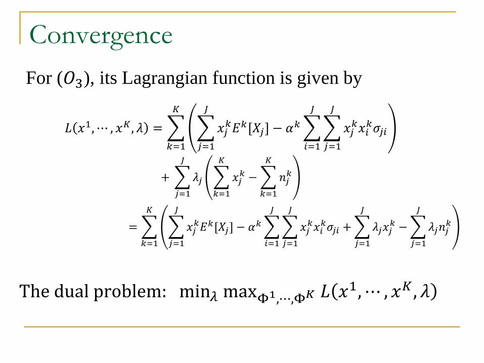
Convergence
For (𝑂3), its Lagrangian function is given by
𝐿 𝑥1, ⋯ , 𝑥𝐾, 𝜆 =
𝑘=1
𝐾
𝑗=1
𝐽
𝑥𝑗𝑘𝐸𝑘[𝑋𝑗] − 𝛼𝑘
𝑖=1
𝐽
𝑗=1
𝐽
𝑥𝑗𝑘𝑥𝑖
𝑘𝜎𝑗𝑖
+
𝑗=1
𝐽
𝜆𝑗
𝑘=1
𝐾
𝑥𝑗𝑘 −
𝑘=1
𝐾
𝑛𝑗𝑘
=
𝑘=1
𝐾
𝑗=1
𝐽
𝑥𝑗𝑘𝐸𝑘[𝑋𝑗] − 𝛼𝑘
𝑖=1
𝐽
𝑗=1
𝐽
𝑥𝑗𝑘𝑥𝑖
𝑘𝜎𝑗𝑖 +
𝑗=1
𝐽
𝜆𝑗𝑥𝑗𝑘 −
𝑗=1
𝐽
𝜆𝑗𝑛𝑗𝑘
The dual problem: min𝜆 maxΦ1,⋯,Φ𝐾 𝐿 𝑥1, ⋯ , 𝑥𝐾 , 𝜆

Convergence
Theorem 2. Let 𝜆∗ be the optimal solution to the
dual problem, then there exists an equilibrium price
vector given by 𝑃∗ = −𝑝0𝜆∗.

Convergence
Denote 𝑔 𝜆 as the subjective function of the dual:
𝑔 𝜆 = max𝑥1,⋯,𝑥𝐾 𝐿 𝑥1, ⋯ , 𝑥𝐾 , 𝜆
Then we can use the following subgradient algorithm
to search for the optimal 𝜆∗:
𝜆𝑛+1 = 𝜆𝑛 − 𝑎𝑛𝑑𝑛/ 𝑑𝑛
where 𝑑𝑛 is a subgradient of 𝑔 𝜆 , which can be
taken as:
𝑑𝑛 =𝑘=1
𝐾
𝑥𝑛𝑘 −
𝑘=1
𝐾
𝑁𝑘

Extensions
𝑥𝑗𝑘 may be constrained, e.g., 𝑥𝑗
𝑘 ≥ 0
σ𝑗=1𝐽
𝑥𝑗𝑘𝑝𝑗 + 𝑥0
𝑘𝑝0 = σ𝑗=1𝐽
𝑛𝑗𝑘𝑝𝑗 + 𝑛0
𝑘𝑝0 may
be modified as
The objective function could be more general
…
𝑗=1
𝐽
𝑚𝑗𝑘𝑥𝑗
𝑘− + 𝑥𝑗𝑘+ 𝑝𝑗 + 𝑥0
𝑘𝑝0 =
𝑗=1
𝐽
𝑛𝑗𝑘𝑝𝑗 + 𝑛0
𝑘𝑝0
Recommended