THE CONDITION OF QUADRATIC AND CUBIC BEZIER CURVES TO
TOUCH A CONSTRAINT LINE
by
FUZIATUL NORSYIHA BINTI AHMAD SHUKRI
Dissertation submitted in partial fulfillment
of the requirements for the degree
of Master of Science in Mathematics
June 2010

ACKNOWLEDGEMENT
I would like to setze this opportunity to express my deepest gratitude to my
supervisor, Pn Ena bt Jamal for her guidance and support throughout this work.
Without her guidance and drive, I would never have completed this dissertation.
Also, I would like to thank Prof. Madya Dr J amaludin Md Ali for his guidance and
suggestion which had really improved the quality of this work. Besides that, I would
like to express my appreciation to all the staff of Mathematical School, course mates
and friends for their constant encouragement and best wishes.
Finally, my very special thanks go to my parents for their financial support and
endless moral support throughout the preparation of this dissertation. I would not
have accomplished my goal without all of you.
Thank you.
ii
CONTENTS
Acknowledgement
Contents
List of Figures
Abstrak
Abstract
Chapter 1: Introduction
1.1 Background of CAGD
1.2 Statement ofProblem
1.3 Literature Review
1.4 Objective ofDissertation
1.5 Scope of Study
1.6 Significance of Study
1.7 Summary and Structure
Chapter 2: Introduction of Bezier Curve
2.1 Bernstein Polynomial
2.1.1 Bernstein Polynomial Degree 1
2.1.2 Bernstein Polynomial Degree 2
iii
11
111
Vll
lX
X
1
1
2
2
3
3
3
4
6
6
6
7
2.1.3 Bernstein Polynomial Degree 3 8
2.2 Properties of Bernstein Polynomial 9
2.2.1 Endpoints 9
2.2.2 Recursion 10
2.2.3 Non-Negativity 10
2.2.4 Symmetry 11
2.2.5 Derivatives 11
2.3 Bezier Curve 12
2.3.1 Linear Bezier Curve 13
2.3.2 Quadratic Bezier Curve 14
2.3.3 Cubic Bezier Curve 15
2.4 Properties ofBezier Curve 17
2.4.1. Endpoint Interpolation 17
2.4.2 Designing ofBezier Polygon 17
2.4.3 Bezier Curve Derivative 18
2.5 Matrix Formulation Bezier Curve 19
Chapter 3: Condition of Quadratic Bezier Curve to Touch a Constraint Line 21
3.1 Introduction 21
3.2 Condition for Quadratic Bezier Curve to Touch a Constraint Line 21
3.2.1 Case I: The Constraint Line is the x-Axis
3.2.2 Case II: The Constraint Line is Any Straight Line
21
23
3.3 Algorithm 25
3.3.1 Condition for Quadratic Bezier Curve to Touch the x-Axis 25
3.3.2 Condition for Quadratic Bezier curve to Touch Any Straight Line 25
3.4 Graphical Results 26
iv
3.4.1 Quadratic Bezier Curve Touching the x-Axis 27
3.4.2 Quadratic Bezier Curve Touching Any Straight Line 29
Chapter 4: Condition of Cubic Bezier Curve to Touch a Constraint Line 32
4.1 Introduction 32
4.2 Condition for Cubic Bezier Curve to Touch a Constraint Line 32
4.2.1 Case 1: The Constraint Line is the x-Axis
4.2.2 Case II: The Constraint Line is Any Straight Line
4.3 Algorithm
4.3.1 Condition for Cubic Bezier Curve to Touch thex-Axis
32
35
38
38
4.3.2 Condition for Cubic Bezier Curve to Touch Any Straight Line 39
4.4 Graphical Results
4.4.1 Cubic Bezier Curve Touching the x-Axis
4.4.1.1 C-shape
4.4.1.2 S-shape
4.4.2 Cubic Bezier curve touching Any Straight Line
Chapter 5: Applications
5.1 Application ofBezier Curve
5.2 Application ofBezier Curve and Constraint Line
5.2.1 Graphical Results
Chapter 6: Conclusion
6.1 Conclusion
6.2 Future Work
Bibliography
v
39
40
40
42
44
46
46
48
51
53
53
55
56
Appendixes
Appendix A: Quadratic Bezier Curve Touching the x-Axis
Appendix B: Quadratic Bezier Curve Touching Any Straight Line
Appendix C: Cubic Bezier Curve Touching the x-Axis (C-shape)
Appendix D: Cubic Bezier Curve Touching the x-Axis (S-shape)
Appendix E: Cubic Bezier Curve Touching Any Straight Line
vi
58
60
63
67
71
LIST OF FIGURES
Figure 2.1 Bernstein polynomial of degree 1 7
Figure 2.2 Bernstein polynomial of degree 2 8
Figure 2.3 Bernstein polynomial of degree 3 9
Figure 2.4 Bezier curve of degree 1 13
Figure 2.5 Bezier curve of degree 2 14
Figure 2.6 Bezier curve of degree 3 15
Figure 2.7 Other example of cubic Bezier curve 16
Figure 2.8 Example of Convex Bezier curve/ C-shape 17
Figure 2.9 Example ofBezier curve with an inflection point/ S-shape 18
Figure 3.1 Quadratic Bezier curve touching the x-axis without control polygon 27
Figure 3.2 Quadratic Bezier curve touching the x-axis with control polygon 27
Figure 3.3 Quadratic Bezier curve touching the x-axis without control polygon 28
Figure 3.4 Quadratic Bezier curve touching the x-axis with control polygon 28
Figure 3.5: Quadratic Bezier curve touching straight line without control polygon 29
Figure 3.6: Quadratic Bezier curve touching straight line with control polygon 29
Figure 3.7: Quadratic Bezier curve touching straight line without control polygon 30
vii
Figure 3.8 Quadratic Bezier curve touching straight line with control polygon 30
Figure 4.1 Cubic Bezier curve touching the x-axis without control polygon (C-shape) 40
Figure 4.2 Cubic Bezier curve touching the x-axis with control polygon (C-shape) 40
Figure 4.3 Cubic Bezier curve touching the x-axis without control polygon (C-shape) 41
Figure 4.4 Cubic Bezier curve touching the x-axis with control polygon (C-shape) 41
Figure 4.5 Cubic Bezier curve touching the x-axis without control polygon (S-shape) 42
Figure 4.6 Cubic Bezier curve touching the x-axis with control polygon (S-shape) 42
Figure 4.7 Cubic Bezier curve touching the x-axis without control polygon (S-shape) 43
Figure 4.8 Cubic Bezier curve touching the x-axis with control polygon (S-shape) 43
Figure 4.9 Cubic Bezier curve touching straight line without Control polygon 44
Figure 4.10 Cubic Bezier curve touching straight line with control polygon 44
Figure 4.11 Cubic Bezier curve touching straight line without control polygon 45
Figure 4.12 Cubic Bezier curve touching straight line with control polygon 45
Figure 5.1 Aladdin drawing 47
Figure 5.2 Robot motion through point (3, 3) 51
Figure 5.3 Robot motion through point (4, 4) 52
viii
SYARAT BAGI LENGKUNG BEZIER KUADRATIK DAN KUBIK UNTUK MENYENTUH GARIS KEKANGAN
ABSTRAK
Bezier merupakan satu daripada polinomial yang paling berpengaruh untuk
interpolasi. Interpolasi lengkung Bezier selalu berada di dalam hull cembung titik
kawalan dan tidak pemah bergerak terlampau jauh dari titik kawalan. Interpolasi
polinomial Bezier mempunyai aplikasi yang sangat luas kerana ia senang untuk
dikira dan sangat stabil.
Di dalam disertasi ini, kami menyelidik syarat lengkung Bezier kuadratik dan kubik
untuk menyentuh garis kekangan. Jadi, titik kawalan memainkan peranan penting
untuk mencapai matlamat ini kerana titik kawalan boleh bergerak ke seluruh arah
dan memberikan pelbagai bentuk lengkung Bezier. Walaubagaimanapun, titik
kawalan pertama dan terakhir akan diberikan dalam disertasi ini. Oleh itu, hanya titik
kawalan di tengah sahaja yang akan mengubah bentuk bagi setiap lengkung Bezier
ini. Oleh hal demikian, bagi menentukan syarat lengkung Bezier kuadratik dan kubik
untuk menyentuh garis kekangan, kami perlu mencari lokasi setiap titik kawalan
yang berada di tengah lengkung Bezier supaya lengkung Bezier hanya menyentuh
tetapi tidak melepasi garis kekangan.
ix
ABSTRACT
Bezier is one of the most influential polynomial representations for interpolation.
The Bezier interpolating curve always lies within the convex hull of its control points
and it never oscillates wildly away from the control points. Bezier polynomial
interpolation has wide applications because it is easy to compute and is also very
stable.
In this dissertation, discussion is made on the conditions for quadratic and cubic
Bezier curve to touch a constraint line. Thus, control points play important role in
order to achieve this goal because control points can oscillate and will illustrate a
various shape of Bezier curve. However, the first control point and the last control
point of quadratic and cubic Bezier curve will be given in this dissertation. Hence,
only the middle control point will change the whole shape of each Bezier curve.
Therefore, in order to determine the condition of quadratic and cubic Bezier curve so
as to touch a constraint line, the location of each middle control points has to be
identified so that the curve will only touch the constraint line but without crossing it.
X
CHAPTER!
INTRODUCTION
1.1 Background
Computer Aided Geometric Design (CAGD) is a branch of applied mathematics
concerned with algorithms for the design of smooth curves and surfaces and for their
efficient mathematical representations. The representations are used for the
computation of curves and surfaces, as well as geometrical quantities of importance
such as curvatures, intersections curves between two surfaces and offset surfaces
(Joy, 2000).
The Bezier curve is an important part of almost every computer graphics illustration
program and Computer Aided Geometric Design (CAGD) system in use today. It is
used in many ways, from designing the curves and surfaces of automobiles until to
defining the shape of letters in type fonts. Since it is numerically and the most stable
of all the polynomial-based curves used in these applications, the Bezier curve is an
ideal standard for representing the more complex piecewise polynomial curve
(Mortenson, 1999). Besides, in vector graphics, a Bezier curve is an important tool
used to model smooth curves that can be scaled indefinitely. Bezier curves are also
used in animation as a tool to control motion (Wikipedia, 2010).
1
The Bezier curves were first developed independently by two Frenchmen, Paul de
Casteljau and Pierre Bezier at two car companies, Renault and Citroen, during the
period 1958-1960 (Farin & Hansford, 2000). In 1970, R.Forrest discovered the
connection between the Bezier's work and Bernstein polynomials. The underlying
mathematical theory of Bezier' s work is based on the concept of Bernstein
polynomials.
1.2 Statement of Problem
In this dissertation, a discussion is made on how to generate a Bezier curve so that it
touches a given constraint line. However, there are some conditions that need to be
considered in order to generate the curve. So, these conditions have to be determined
so that a Bezier curve will touch any given constraint line.
1.3 Literature Review
In the case of constrained interpolation, Goodman et al. (1991) had proposed a
scheme for the construction of a G2 parametric interpolating curve which lies on the
same side of a given set of constraint lines as the data. The interpolant is actually a
parametric rational cubic Bezier curve. Meek et al. (2003), extended this result to
generate the curve for a given set of ordered planar points lying on one side of a
polyline, a planar G2 interpolating curve to these data which lies on the same side of
the polyline as data. After that, Jeok and Ong (2006) generated G1 curves which are
constrained to lie on the same side of the given constraint lines as the data and the
interpolant is actually a parametric cubic Bezier-like curve. They also did a
2
modification so that the curve from across the given line would just touch the given
line.
1.4 Objectives of Dissertation
The objectives of this dissertation are:
• to determine the condition of quadratic Bezier curve so that it can touch a
constraint line.
• to determine the condition of cubic Bezier curve so that it can touch a
constraint line.
• to show the application ofBezier curve with a constraint line.
1.5 Scope of Study
This study will investigate the condition of quadratic and cubic Bezier curve in order
to touch a constraint line where the constraint line is x-axis and any straight line
where the tangent slope of the straight line is positive or m ? 0. In addition, the first
control point and the last control point will be of positive values and they will be
provided.
1.6 Significance of Study
This study is useful for those who are interested to do animation films or to make
advertisements in animation.
3
1. 7 Summary and Structure of Dissertation
This dissertation consists of six chapters and the summary of the major contribution
of this dissertation is as follows:
Chapter 1 presents a brief account of Computer Aided Geometry Design (CAGD)
and the background of Bezier Curve. The objectives of the dissertation, statement of
problem, literature review, scope of study and the significance of this dissertation are
also included in this chapter.
Chapter 2 is a brief introduction of Bezier curve. It also explains some properties of
Bernstein polynomial and Bezier curve for degree one, degree two and degree three.
The graphical examples of Bernstein polynomial and Bezier curve are also presented
in this chapter.
Chapter 3 focus on ways of determining the condition of quadratic Bezier curve in
order to touch a constraint line. First, the focus is on ways of determining the
condition of quadratic Bezier curve in order to touch a constraint line where the
constraint line is the x-axis. Next, this is extended to the case where the constraint
line can be of any straight line.
Chapter 4 focuses on ways of determining the condition of cubic Bezier curve in
order to touch a constraint line. First, the focus is on ways of determining the
condition of cubic Bezier curve in order to touch a constraint line where the
4
constraint line is the x-axis. This is then extended to the case where the constraint
line can be of any straight line.
Chapter 5 demonstrates some applications of the Bezier curve which is a 2D drawing
produced through the combination ofBezier curves of different degrees. Besides, this
chapter also illustrates the applications of the Bezier curve and a constraint line
which can be applied in a robotic motion and parabolic wall.
Chapter 6 is the conclusion and some recommendations of this dissertation are
discussed in this chapter.
5
CHAPTER2
INTRODUCTION OF BEZIER CURVE
2.1 Bernstein Polynomials
The Bernstein polynomials of degree n are defined as
O::;t::;1
for i = 0, 1, ... , n, where the binomial coefficients are given by
(n) n! i = i!(n-i)!
if 0 ::; i ::; n
and for mathematical convenience, it is usually set as Br = 0 if i < 0 or i > n.
These polynomials are quite simple to be written down. The coefficient (7) can be
obtained from Pascal's triangle where the exponents on the t term increases by one
as i increases and the exponents on the ( 1 - t) term decreases by one as i increases
(Joy, 2000).
2.1.1 Bernstein Polynomial of Degree 1
=1-t
6
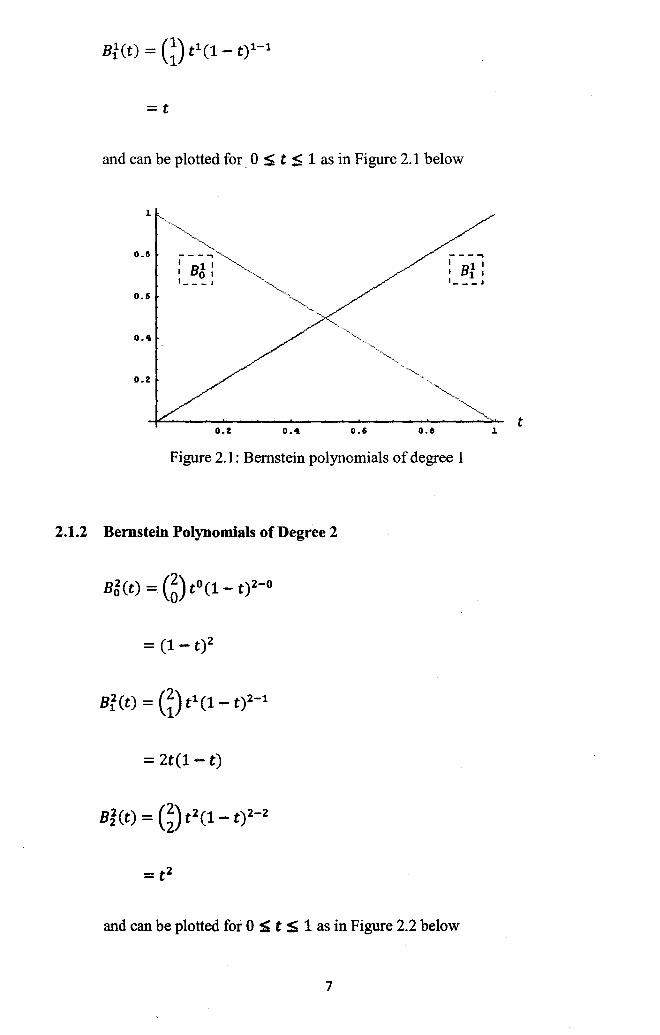
=t
and can be plotted for. 0 :s; t ::;; 1 as in Figure 2.1 below
---"""' I 1 I I Bt I I_-- J
o.t
t O.t 0.4 0.6 0.11 l.
Figure 2.1: Bernstein polynomials of degree 1
2.1.2 Bernstein Polynomials of Degree 2
= 2t(1- t)
= t~
and can be plotted for 0 S t S 1 as in Figure 2.2 below
7
l.
0.0
0.11
0.4:
o.z
-----. I 2 I I Bo I I_-- J
0.2: 0.4:
---"""') I 2 I I Bt I I_-- J
·-~ ·--.... -"'-....
-----I 2 I 1 8 2 1 I_-- J
-------~-~~-~---
0.11 0.0
Figure 2.2: Bernstein polynomials of degree 2
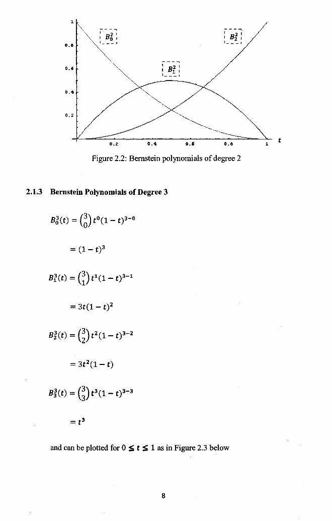
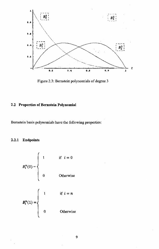
2.1.3 Bernstein Polynomials of Degree 3
= (1- t) 3
= 3t(1- t)2
and can be plotted for 0 S t S 1 as in Figure 2.3 below
8
l. t
l.
0.0
0.15
0.4
----. I 3 1 I 81 I I_--'
0.2 0.4 0.15
----; I 3 I I 83 1 ! - <-- J
0.0
----a I • 3 1 I 82 1 I_-- J
Figure 2.3: Bernstein polynomials of degree 3
2.2 Properties of Bernstein Polynomial
Bernstein basis polynomials have the following properties:
2.2.1 Endpoints
1 if i = 0
0 Otherwise
1 if i = n
0 Otherwise
9
t l.
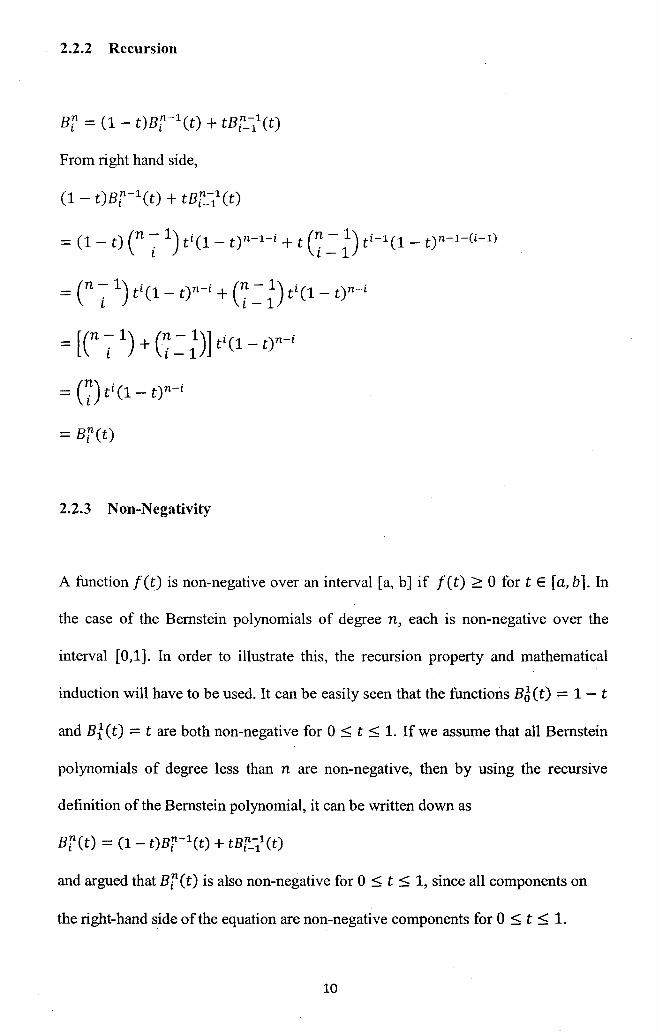
2.2.2 Recursion
Bi = (1- t)Bi-1(t) + tBi--~/(t)
From right hand side,
(1- t)Bi-1(t) + tBi_-~/(t)
= (1- t) (n ~ 1) ti(1- t)n-1-i + t (7 ~ ~) ti-1(1- t)n-1-(i-1)
= (n ~ 1) ti(1- t)n-i + (7 ~ ~) ti(1- t)n-i
= [(n~1)+(7~~)]ti(1 -t)n-i
= (7) ti (1- t)n-i
= Bi(t)
2.2.3 Non-Negativity
A function f(t) is non-negative over an interval [a, b) if f(t) ;:::: 0 fortE [a, b]. In
the case of the Bernstein polynomials of degree n, each is non-negative over the
interval [0,1 ]. In order to illustrate this, the recursion property and mathematical
induction will have to be used. It can be easily seen that the functions BJ(t) = 1- t
and B.f(t) =tare both non-negative for 0:::; t:::; 1. If we assume that all Bernstein
polynomials of degree less than n are non-negative, then by using the recursive
definition of the Bernstein polynomial, it can be written down as
Bi(t) = (1- t)B[-1(t) + tBf_-/(t)
and argued that Bi(t) is also non-negative for 0 :::; t < 1, since all components on
the right-hand side of the equation are non-negative components for 0 :::; t :::; 1.
10
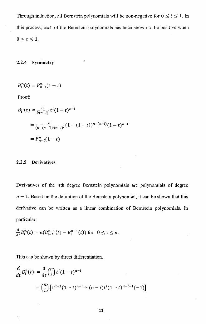
Through induction, all Bernstein polynomials will be non-negative for 0 ~ t ~ 1. In
this process, each of the Bernstein polynomials has been shown to be positive when
O~t~l.
2.2.4 Symmetry
srct) = s:;_i(1- t)
Proof:
B!l(t) = _n_! -ti(1- t)n-i t i!(n-i)!
= n! (1- (1- t))n-(n-i)(1- t)n-i (n-(n-i))!(n-i)!
= sn ·(1- t) n-t
2.2.5 Derivatives
Derivatives of the nth degree Bernstein polynomials are polynomials of degree
n - 1. Based on the definition of the Bernstein polynomial, it can be shown that this
derivative can be written as a linear combination of Bernstein polynomials. In
particular:
:t sr(t) = n(Bf_-~/(t)- sr-1 (t)) for o ~ i ~ n.
This can be shown by direct differentiation.
d d (n) . . -B!I(t) =- . tt(1- t)n-t dt t dt l
11
= n(n-1)! ti-1(1- t)n-i- n(n-1)! ti(1- t)n-i-1 (i-1)!(n-i)! i!(n-i-1)!
= n ( (n-1)! ti-1(1- t)n-i- (n-1)! ti(1- t)n-i-1) (i-1)!(n-i)! i!(n-i-1)!
2.3 Bezier Curves
By using the Bernstein basis functions, the Bezier polynomial of degree n can be
defined as:
n
P(t)= 'LC;B;n(t), O~t~1 ;~o
with coefficients ci E RT(r = 1,2,3).
If Ci are vectors in R 2 or R 3 , then
• Ci are called as a Bezier points or control points of curve and
• P(t) is a curve in the parametric form.
If Ci are real numbers R1 , then
• Ci are named as Bezier ordinates and
• P ( t) is a Bezier function of the variable t with Bezier points (!.., ca. n
The polygon C0 C1 ... Cn formed by connecting the Bezier points with line segments is
called Bezier polygon or control polygon of the curve.
12
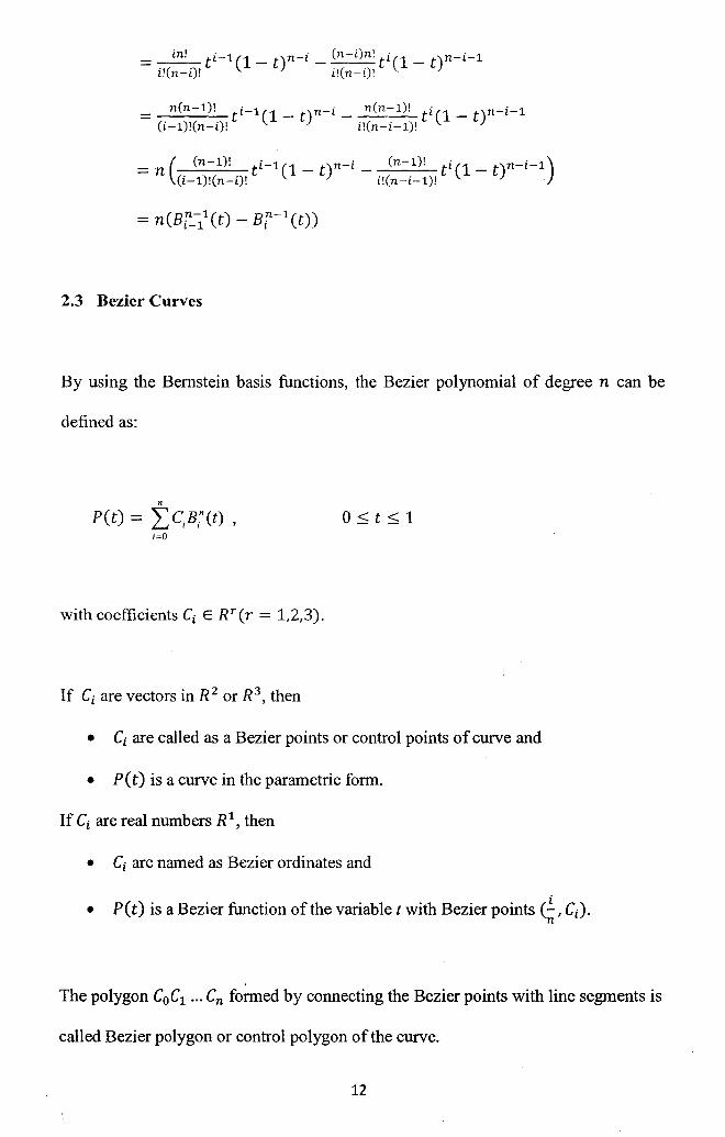
2.3.1 Linear Bezier Curve
Bezier curve of Degree 1 is written as:
Bfi(t) = 1- t
Bt(t) = t
P(t) = (1- t)Co + tC1
4.0
3.5
3.0
:u
1.5 :u 2.5 3.0 3 . .S
Figure 2.4: Bezier curve of degree 1
• '
4.0
Figure 2.4 shows a straight line segment from C0 to C1 (a linear interpolation) and
the curve lies in the convex hull of the Bezier polygon.
13
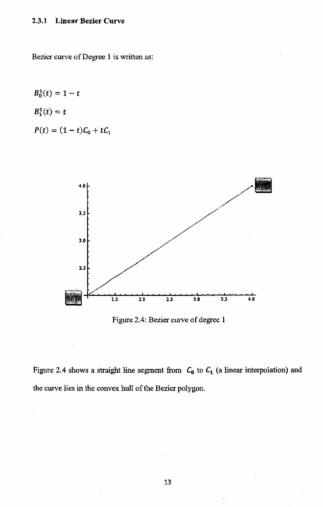
2.3.2 Quadratic Bezier Curve
Bezier curve of Degree two is written as:
B5(t) = (1- t) 2
Bf(t) = 2t(1- t)
Bi(t) = t 2
P(t) = (1- t) 2C0 + 2t(1- t)C1 + t 2C2
s
Figure 2.5: Bezier curve of degree 2
Figure 2.5 shows a parabolic arc from C0 to C2 . The control polygon in Figure 2.5 is
approximately the shape of the Bezier curve and the curve lies within the convex hull
of the Bezier polygon.
14
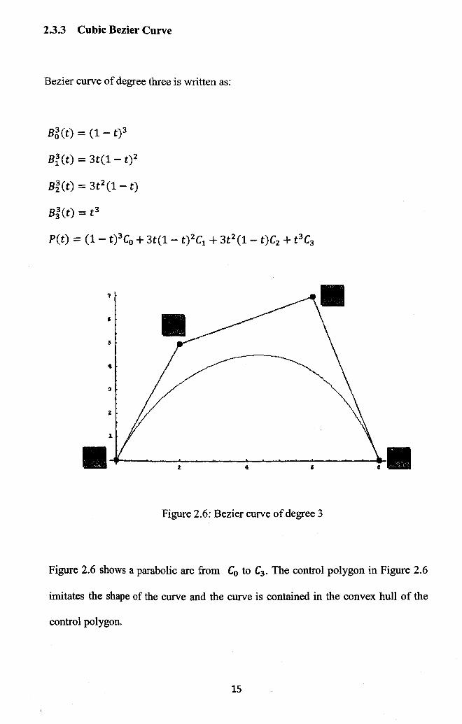
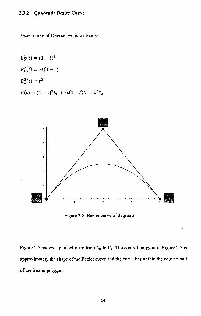
2.3.3 Cubic Bezier Curve
Bezier curve of degree three is written as:
Bg(t) = (1- t) 3
Bi(t) = 3t(1- t) 2
B~(t) = 3t2 (1- t)
Bj(t) = t 3
P(t) = (1- t) 3 Co + 3t(1- t) 2 C1 + 3t2 (1- t)C2 + t 3 C3
Figure 2.6: Bezier curve of degree 3
Figure 2.6 shows a parabolic arc from C0 to C3 . The control polygon in Figure 2.6
imitates the shape of the curve and the curve is contained in the convex hull of the
control polygon.
15
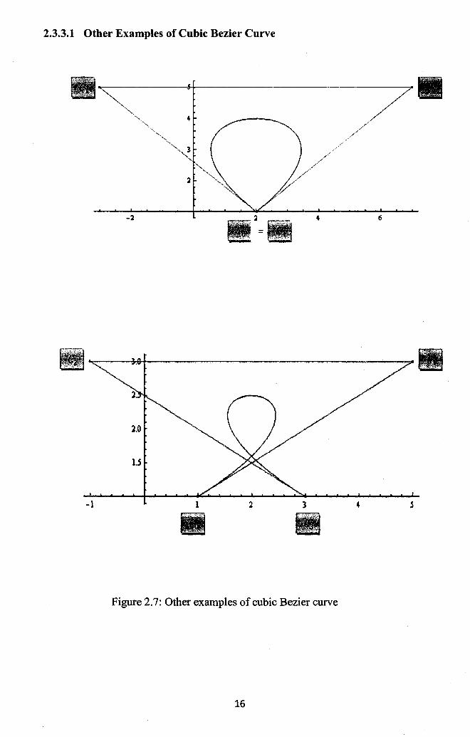
2.3.3.1 Other Examples of Cubic Bezier Curve
-1
'"'-~-""""'--,_ ·,·,,"" 4
'·"'--, 3
-2
l.O
1.5
4
3
Figure 2.7: Other examples of cubic Bezier curve
16
4 5
2.4 Properties of Bezier Curve
The Bezier curve has the following properties:
2.4.1 Endpoint Interpolation
The Bezier curve P(t) always passes through the first control point C0 and the last
control points Cn·
n
P(O) = L (B;n (0) = Co, i=O
n
P(1) = L(B;n (1) = Cn. i=O
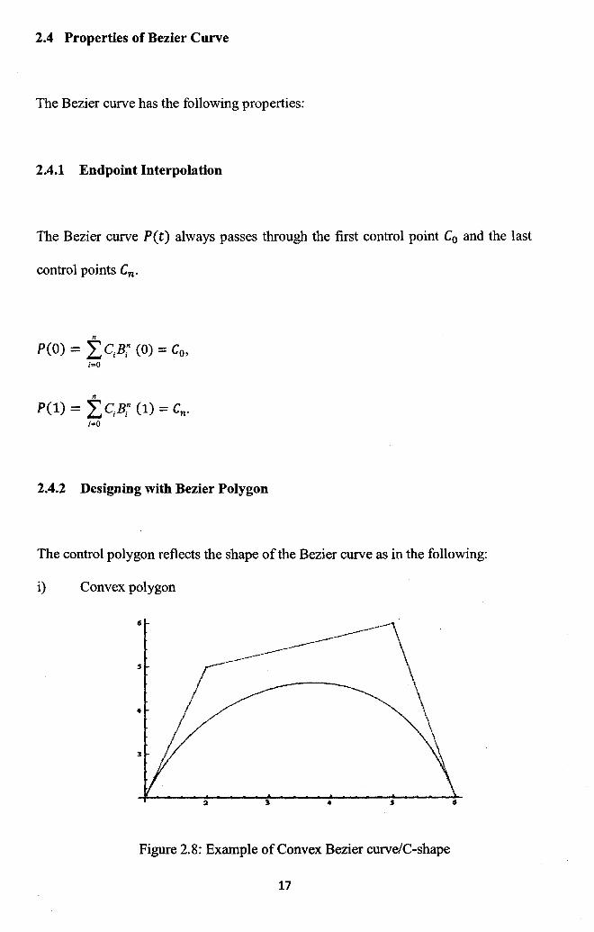
2.4.2 Designing with Bezier Polygon
The control polygon reflects the shape of the Bezier curve as in the following:
i) Convex polygon
Figure 2.8: Example of Convex Bezier curve/C-shape
17
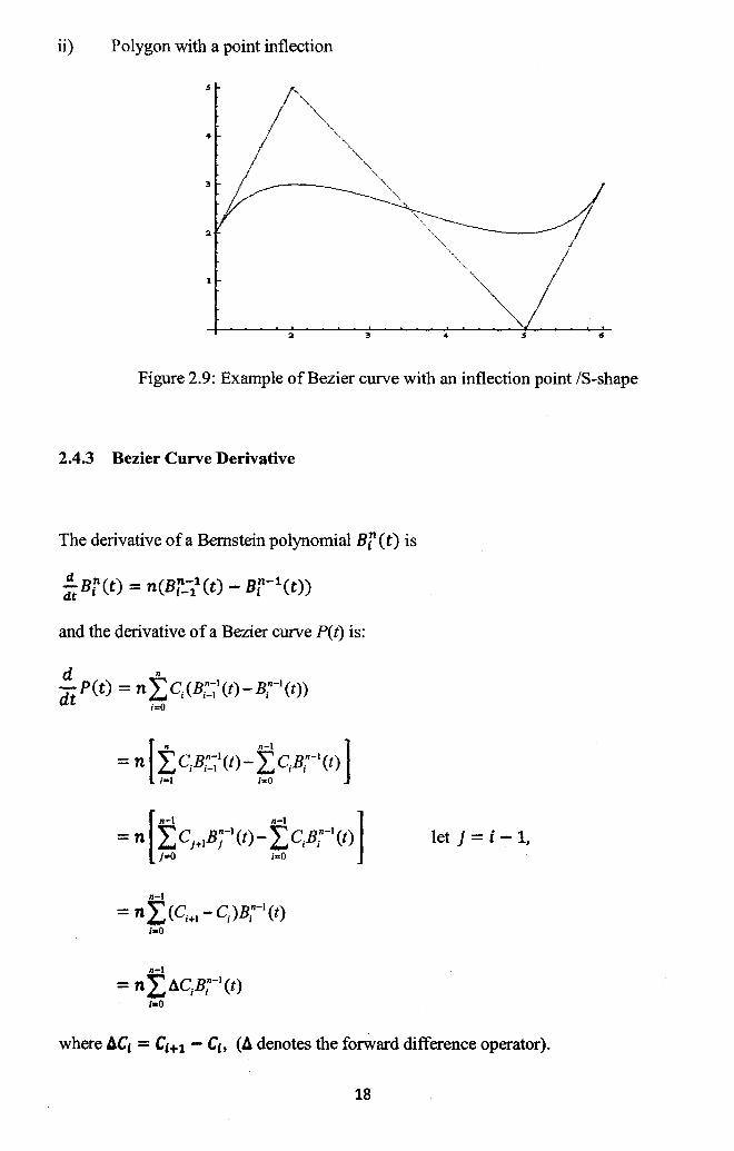
ii) Polygon with a point inflection
3 ..
Figure 2.9: Example ofBezier curve with an inflection point IS-shape
2.4.3 Bezier Curve Derivative
The derivative of a Bernstein polynomial Br(t) is
and the derivative of a Bezier curve P(t) is:
let j = i -1,
n-1
= n L ( ci+l - C1 )Bt-l (t) i•O
n-1
= n L ACIBin-1 (t) i•O
where ACt = Ct+l - Ch (A denotes the forward difference operator).
18
2.5 Matrix Formulation of Bezier Curve
A Bezier curve can be written in a matrix form by expanding the analytic definition
of the curve into its Bernstein polynomial coefficients, and then writing these
coefficients in a matrix form by using the polynomial power basis.
2.5.1 Quadratic Bezier Curve
2
The quadratic Bezier curve is P(t) = L C;B;2 (t) or it can be re-written as: ;~o
= [(1- t) 2 2t(1- t)
= [1 t t 2] M [m
whereM= H 0
H 2 -2
Let T = [1 t t 2 ] and C = [~~]· Hence, the matrix representation of quadratic
Bezier curve is
P(t) = TMC
= [1 t t2] H J mm .
19
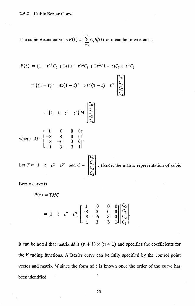
2.5.2 Cubic Bezier Curve
3
The cubic Bezier curve is P(t) = I C;B;3(t) or it can be re-written as: ;~o
= ((1 - t) 3 3t(1- t) 2 3t2 (1- t) t 3] [~~]
r
1 -3 where M=
3 -1
0 3
-6 3 JH
Let T ~ [1 t t 2 t 3] and C ~ [~;1· Hence, the matrix representation of cubic
Bezier curve is
P(t) = TMC
= [1 t t 2
0 0 3 0
-6 3 3 -3
It can be noted that matrix M is (n + 1) X (n + 1) and specifies the coefficients for
the blending functions. A Bezier curve can be fully specified by the control point
vector and matrix M since the form of t is known once the order of the curve has
been identified.
20
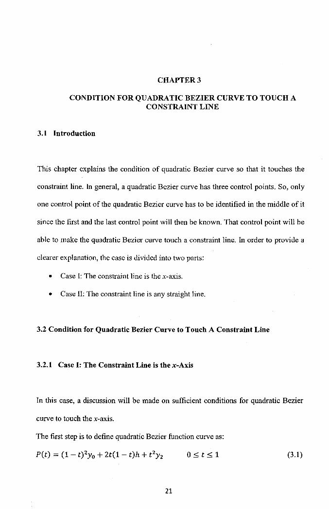
CHAPTER3
CONDITION FOR QUADRATIC BEZIER CURVE TO TOUCH A CONSTRAINT LINE
3.1 Introduction
This chapter explains the condition of quadratic Bezier curve so that it touches the
constraint line. In general, a quadratic Bezier curve has three control points. So, only
one control point of the quadratic Bezier curve has to be identified in the middle of it
since the first and the last control point will then be known. That control point will be
able to make the quadratic Bezier curve touch a constraint line. In order to provide a
clearer explanation, the case is divided into two parts:
• Case I: The constraint line is the x-axis.
• Case ll: The constraint line is any straight line.
3.2 Condition for Quadratic Bezier Curve to Touch A Constraint Line
3.2.1 Case I: The Constraint Line is the x-Axis
In this case, a discussion will be made on sufficient conditions for quadratic Bezier
curve to touch the x-axis.
The first step is to define quadratic Bezier function curve as:
o:::;t<l (3.1)
21
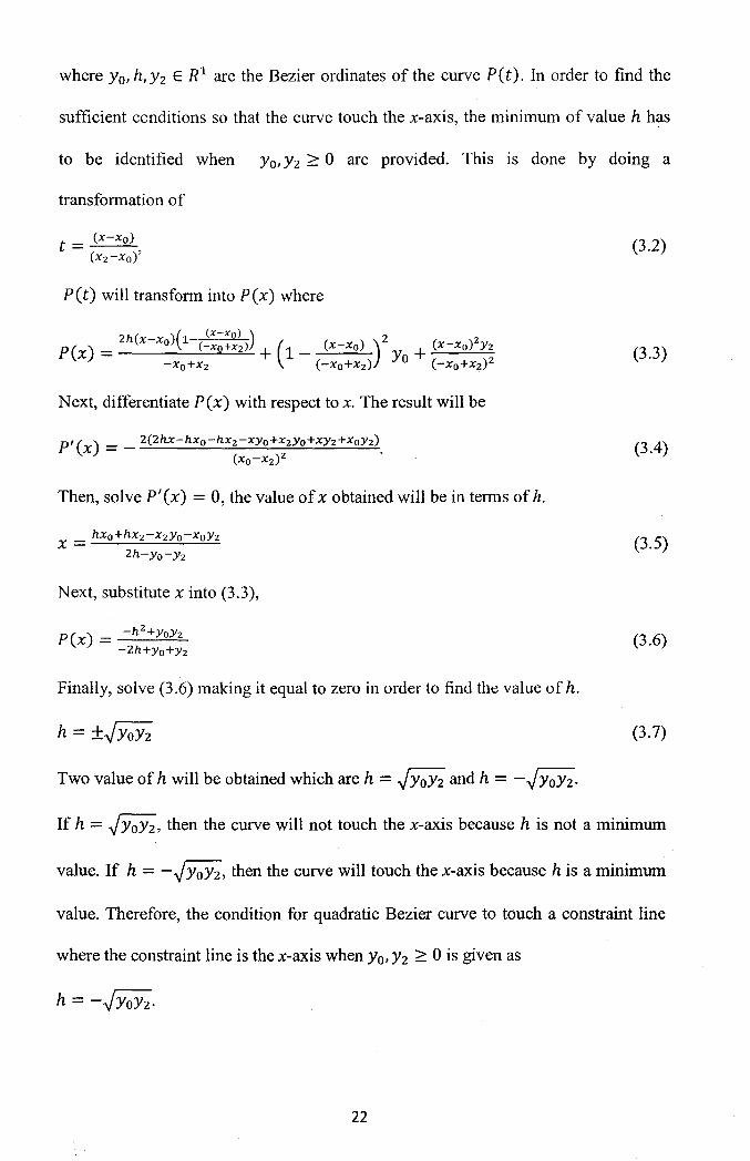
where y 0 , h, y 2 E R 1 are the Bezier ordinates of the curve P ( t). In order to find the
sufficient ccnditions so that the curve touch the x-axis, the minimum of value h has
to be identified when y 0 , y 2 ~ 0 are provided. This is done by doing a
transformation of
t = (x-xo) (xz-Xo)'
P(t) will transform into P(x) where
Zh(x x )(1 (x-xo) ) 2 z P(x) = - 0
(-x0+x2 ) + (l _ (x-xo) ) Yo + (x-xo) Yz -x0+x2 ( -x0+x2 ) ( -x0+xz) 2
Next, differentiate P(x) with respect to x. The result will be
P'(x) = _ Z(Zhx-hxo-hxz-XYo+XzYo+Xyz+XoYz). (xo-Xz)z
Then, solve P'(x) = 0, the value ofx obtained will be in terms of h.
Next, substitute x into (3.3),
Finally, solve (3.6) making it equal to zero in order to find the value of h.
h = ±.JYoYz
Two value of h will be obtained which are h = .Jy0y2 and h = -.JYoYz·
(3.2)
(3.3)
(3.4)
(3.5)
(3.6)
(3.7)
If h = .Jy0y2 , then the curve will not touch the x-axis because his not a minimum
value. If h = -.Jy0y2 , then the curve will touch the x-axis because his a minimum
value. Therefore, the condition for quadratic Bezier curve to touch a constraint line
where the constraint line is the x-axis when y0 , y 2 ~ 0 is given as
h = -.JYoYz·
22
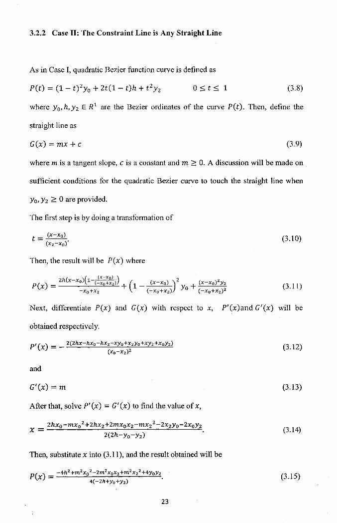
3.2.2 Case II: The Constraint Line is Any Straight Line
As in Case I, quadratic Bezier function curve is defined as
o::;t::; 1 (3.8)
where y 0 , h, y 2 E R1 are the Bezier ordinates of the curve P(t). Then, define the
straight line as
G(x) = mx + c (3.9)
where m is a tangent slope, cis a constant and m 2:: 0. A discussion will be made on
sufficient conditions for the quadratic Bezier curve to touch the straight line when
Yo, Yz > 0 are provided.
The first step is by doing a transformation of
t = (x-xo). (xz-xo)
Then, the result will be P(x) where
2h(x x )(1 (x-xo) ) 2 z P(x) = - 0 (-x0 +x2 ) + (1 _ (x-xo) ) Yo + (x-xo) Yz
-x0 +x2 (-xo+xz) (-x0 +x2 ) 2
(3.1 0)
(3.11)
Next, differentiate P(x) and G(x) with respect to x, P'(x)and G'(x) will be
obtained respectively.
P' (x) = _ 2(2hx-hx0 -hx2 -xy0 +x2 y0 +xy2 +x0 y 2 )
(xo-Xz) 2
and
G'(x) = m
After that, solve P' (x) = G' (x) to find the value of x,
Then, substitute x into (3.11), and the result obtained will be
P(x) = -4hz+mzxoZ-zmZxoXz+mZxzz+4yoYz.
4( -2h+yo+Yz)
23
(3.12)
(3.13)
(3.14)
(3.15)
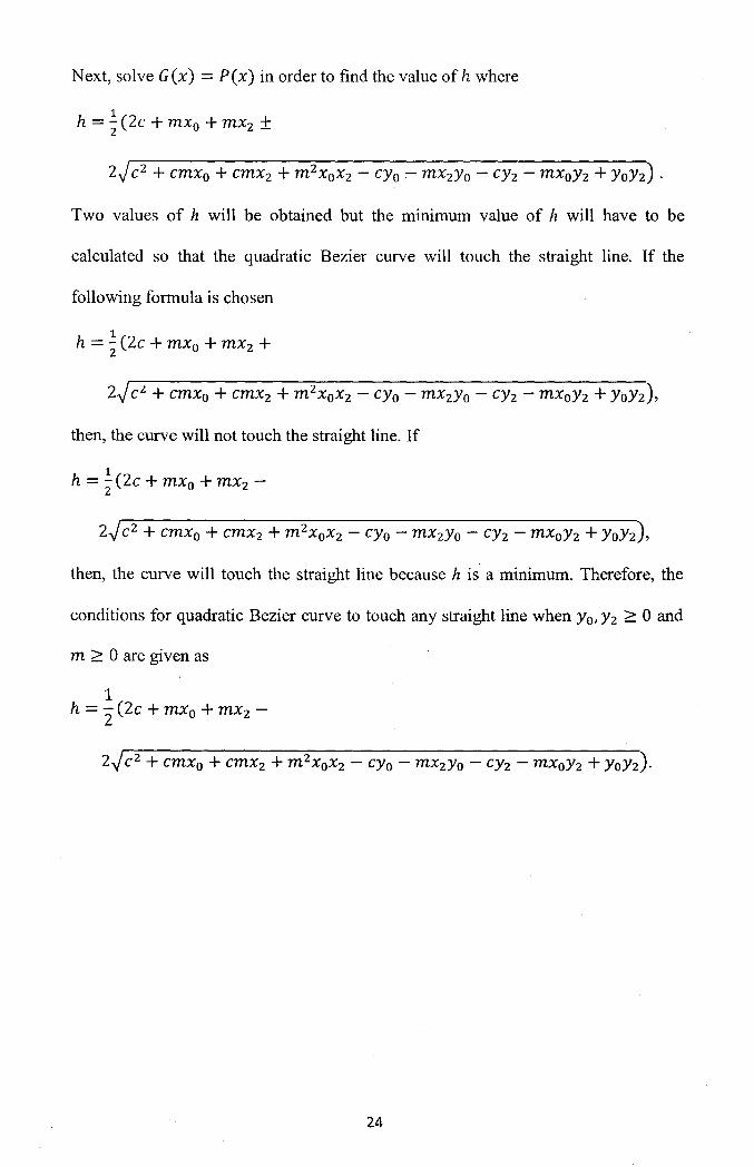
Next, solve G (x) = P ( x) in order to find the value of h where
1 h = 2 (2c + mx0 + mx2 ±
z.J c2 + cmx0 + cmx2 + m2x0 x2 - cyo :- mx2Yo - cy2 - mxoY2 + YoY2) ·
Two values of h will be obtained but the minimum value of h will have to be
calculated so that the quadratic Bezier curve will touch the straight line. If the
following formula is chosen
1 h = - (2c + mx0 + mx2 +
2
z.J cl. + cmx0 + cmx2 + m2XoX2 - CYo - mX2Yo - cy2 - mxoY2 + YoYz),
then, the curve will not touch the straight line. If
1 h = - (2c + mx0 + mx2 -2
z.Jc2 + cmx0 + cmx2 + m2x0 x2 - cy0 - mX2Yo- cy2- mXoY2 + YoY2),
then, the curve will touch the straight line because h is a minimum. Therefore, the
conditions for quadratic Bezier curve to touch any straight line when y0 , y2 ~ 0 and
m ~ 0 are given as
1 h = 2 (2c + mx0 + mx2 -
2.Jc2 + cmx0 + cmx2 + m 2x0x2 - cy0 - mx2Yo- cy2- mxoY2 +YoY2).
24
Recommended