The Cause of Housing Market
Fluctuations in ChinaAn Indirect Inference Perspective
Yue Gai
Supervisor: Prof. Patrick Minford
Dr Zhirong Ou
Economics Department
Cardiff University
A Thesis Submitted in Fulfilment of the Requirements for the
Degree of Doctor of Philosophy of Cardiff University
Cardiff Business School May 2019


Declaration
I hereby declare that except where specific reference is made to the work of others, the
contents of this dissertation are original and have not been submitted in whole or in part
for consideration for any other degree or qualification in this, or any other university. This
dissertation is my own work and contains nothing which is the outcome of work done in
collaboration with others, except as specified in the text and Acknowledgements. This
dissertation contains fewer than 65,000 words including appendices, bibliography, footnotes,
tables and equations and has fewer than 150 figures.
Yue Gai
May 2019


Acknowledgements
This thesis becomes a reality with the kind support and help of many individuals. I would
like to extend my sincere thanks to all of them.
First and foremost, I would like to express my sincere gratitude to my supervisor Prof.
Patrick Minford for the continuous support of my PhD study and research, for his patience,
motivation, enthusiasm and immense knowledge. Also, thank him for providing me with a
full PhD scholarship. I would also like to thank my secondary supervisor, Dr Zhirong Ou for
his encouragement, insightful comments and hard questions.
I thank all my fellow in office B48 for the stimulating discussion, for the days we were
working together before exam and deadlines, and for all the fun we have had in the last five
years. ’The big family’ belong to us. And also thank my friends who support me and help
me in every way.
Last, I would like to dedicate my work to my beloved parents Renlong Gai and Juan
Li for their love, endless support, encouragement and always standing by me. I would also
thank my husband Qiupeng Kong for always believing in me, encourage me and raising me
up when I was feeling down.
As a final word, I would like to thank each and every individual who has been a source
of support and encouragement and helped me to achieve my goal and complete my thesis
successfully.


Abstract
This thesis addresses two main issues related to the housing market in China. It discovers:
i) the key driving forces behind the movements of housing price and the evaluation of
the model’s capacity in fitting the data. ii) try to identify whether the Chinese housing
market can be explained better by using a model with collateral constraint. The Dynamic
Stochastic General Equilibrium (DSGE) model including the housing sector and capturing
some important features of the Chinese economy is employed to explore the above questions.
Moreover, an Indirect Inference method is used to explore these issues in an empirical way.
Estimation results show that the estimated model using Indirect Inference method can explain
the data behaviour well. The estimated model shows that the capital demand shock plays a
significant major role in explaining the housing price dynamic. In terms of the second issue,
the Indirect Inference testing results show that the model with collateral constraint cannot
provide better performance in explaining the data.


Table of contents
List of figures xv
List of tables xvii
1 Introduction 1
1.1 Background and Motivation . . . . . . . . . . . . . . . . . . . . . . . . . 1
1.2 Methodology and Findings . . . . . . . . . . . . . . . . . . . . . . . . . . 4
1.3 Thesis Structure . . . . . . . . . . . . . . . . . . . . . . . . . . . . . . . 6
2 Literature Review 7
2.1 The Source of Housing price Dynamics . . . . . . . . . . . . . . . . . . . 7
2.2 Collateral Constraint . . . . . . . . . . . . . . . . . . . . . . . . . . . . . 15
3 Benchmark Model 21
3.1 Introduction . . . . . . . . . . . . . . . . . . . . . . . . . . . . . . . . . . 21
3.2 Model . . . . . . . . . . . . . . . . . . . . . . . . . . . . . . . . . . . . . 24
3.2.1 Key Features in the Model . . . . . . . . . . . . . . . . . . . . . . 24
3.2.2 The Model Setting . . . . . . . . . . . . . . . . . . . . . . . . . . 27
3.2.3 The Linearised Housing Model . . . . . . . . . . . . . . . . . . . 41
3.3 The Method of Indirect Inference . . . . . . . . . . . . . . . . . . . . . . . 45
3.3.1 Introduction of Indirect Inference . . . . . . . . . . . . . . . . . . 45

xii Table of contents
3.3.2 Indirect Inference Testing . . . . . . . . . . . . . . . . . . . . . . 47
3.3.3 Indirect Inference Estimation . . . . . . . . . . . . . . . . . . . . . 52
3.3.4 The Choice of the Auxiliary Model . . . . . . . . . . . . . . . . . 53
3.4 Data and Calibration . . . . . . . . . . . . . . . . . . . . . . . . . . . . . 57
3.4.1 Description of Data . . . . . . . . . . . . . . . . . . . . . . . . . . 57
3.4.2 The Advantage of Non-stationary data . . . . . . . . . . . . . . . . 58
3.4.3 Calibration . . . . . . . . . . . . . . . . . . . . . . . . . . . . . . 59
3.5 Empirical Results . . . . . . . . . . . . . . . . . . . . . . . . . . . . . . . 62
3.5.1 Estimation . . . . . . . . . . . . . . . . . . . . . . . . . . . . . . 62
3.5.2 Properties of the Model . . . . . . . . . . . . . . . . . . . . . . . . 69
3.6 Conclusion . . . . . . . . . . . . . . . . . . . . . . . . . . . . . . . . . . 78
4 Model with Collateral Constraint 81
4.1 Introduction . . . . . . . . . . . . . . . . . . . . . . . . . . . . . . . . . . 81
4.2 Model . . . . . . . . . . . . . . . . . . . . . . . . . . . . . . . . . . . . . 84
4.3 Estimation . . . . . . . . . . . . . . . . . . . . . . . . . . . . . . . . . . . 92
4.3.1 Data . . . . . . . . . . . . . . . . . . . . . . . . . . . . . . . . . . 92
4.3.2 Calibration . . . . . . . . . . . . . . . . . . . . . . . . . . . . . . 92
4.3.3 Empirical Results . . . . . . . . . . . . . . . . . . . . . . . . . . . 95
4.3.4 Indirect Inference Power Test . . . . . . . . . . . . . . . . . . . . 99
4.3.5 Error Properties on Non-Stationary Data . . . . . . . . . . . . . . . 101
4.4 Standard Analysis . . . . . . . . . . . . . . . . . . . . . . . . . . . . . . . 104
4.4.1 Impulse Response Functions . . . . . . . . . . . . . . . . . . . . . 104
4.4.2 Variance Decomposition . . . . . . . . . . . . . . . . . . . . . . . 109
4.4.3 Historical Decomposition . . . . . . . . . . . . . . . . . . . . . . 113
4.5 Conclusion . . . . . . . . . . . . . . . . . . . . . . . . . . . . . . . . . . 115

Table of contents xiii
5 Conclusion 117
References 121
Appendix A Data 127
Appendix B Impulse Responses of Main Variables 133


List of figures
1.1 The housing price index . . . . . . . . . . . . . . . . . . . . . . . . . . . 2
1.2 The growth rate of housing price . . . . . . . . . . . . . . . . . . . . . . . 3
3.1 China real GDP per capita and pre-crisis trend . . . . . . . . . . . . . . . . 26
3.2 The Principle of testing using indirect inference . . . . . . . . . . . . . . . 51
3.3 Chinese macroeconomic data: 2001Q1 to 2014Q4 . . . . . . . . . . . . . . 57
3.4 Structure Shocks . . . . . . . . . . . . . . . . . . . . . . . . . . . . . . . 67
3.5 Shock Decomposition - Real Housing Price . . . . . . . . . . . . . . . . . 74
3.6 Impulse responses to Housing Demand Shock . . . . . . . . . . . . . . . . 76
3.7 Impulse responses to Monetary Policy Shock . . . . . . . . . . . . . . . . 77
3.8 Impulse responses to Technology shocks in general sector . . . . . . . . . . 78
4.1 Structure Shocks - Model with Collateral Constraint . . . . . . . . . . . . . 104
4.2 Impulse Response to a 0.1 SE Housing Demand Shock . . . . . . . . . . . 106
4.3 Impulse Response to a 0.1 standard error Monetary Policy Shock . . . . . . 107
4.4 Impulse Response to a 0.1 standard error Productivity Shock in General Sector108
4.5 Historical Decomposition of Real Housing Price . . . . . . . . . . . . . . . 114
4.6 Historical Decomposition of Real Consumption . . . . . . . . . . . . . . . 115
B.1 Government Spending Shock . . . . . . . . . . . . . . . . . . . . . . . . . 133
B.2 Preference Shock . . . . . . . . . . . . . . . . . . . . . . . . . . . . . . . 134

xvi List of figures
B.3 Labour Supply Shock . . . . . . . . . . . . . . . . . . . . . . . . . . . . . 134
B.4 Productivity Shock in Housing Sector . . . . . . . . . . . . . . . . . . . . 135
B.5 Labour Demand Shock in General Sector . . . . . . . . . . . . . . . . . . 135
B.6 Capital Demand Shock in General Sector . . . . . . . . . . . . . . . . . . 136
B.7 Capital Demand Shock in Housing Sector . . . . . . . . . . . . . . . . . . 136
B.8 Government Spending Shock . . . . . . . . . . . . . . . . . . . . . . . . . 137
B.9 Preference Shock . . . . . . . . . . . . . . . . . . . . . . . . . . . . . . . 137
B.10 Labour Supply Shock . . . . . . . . . . . . . . . . . . . . . . . . . . . . . 138
B.11 Productivity Shock in Housing Sector . . . . . . . . . . . . . . . . . . . . 138
B.12 Labour Demand Shock in General Sector . . . . . . . . . . . . . . . . . . 139
B.13 Labour Demand Shock in Housing Sector . . . . . . . . . . . . . . . . . . 139
B.14 Capital Demand Shock in General Sector . . . . . . . . . . . . . . . . . . 140
B.15 Capital Demand Shock in Housing Sector . . . . . . . . . . . . . . . . . . 140

List of tables
3.1 Calibrated Coefficients - Benchmark Model . . . . . . . . . . . . . . . . . 61
3.2 Steady state ratios- Benchmark Model . . . . . . . . . . . . . . . . . . . . 62
3.3 Model Coefficients: 2000Q1-2014Q4 . . . . . . . . . . . . . . . . . . . . 65
3.4 Stationarity of Residual . . . . . . . . . . . . . . . . . . . . . . . . . . . . 68
3.5 Estimated Shocks Coefficient . . . . . . . . . . . . . . . . . . . . . . . . . 69
3.6 Variance Decomposition of aggregate variables- Benchmark Model . . . . . 72
4.1 Calibrated Coefficients - Model with Collateral Constraint . . . . . . . . . 94
4.2 Estimated Coefficients - Model with Collateral Constraint . . . . . . . . . . 98
4.3 Comparison of the Testing Results Based on II estimation . . . . . . . . . . 99
4.4 Monte Carlo Power test- 3 variables VARX(1) . . . . . . . . . . . . . . . . 100
4.5 Monte Carlo Power test- 4 variables VARX(1) . . . . . . . . . . . . . . . . 101
4.6 Stationarity of Residual and AR parameters . . . . . . . . . . . . . . . . . 103
4.7 Variance Decomposition of aggregate variables- Collateral Model . . . . . 112
A.1 Data Description and Source of Benchmark Model . . . . . . . . . . . . . 128
A.2 Data Description and Source of Model with Collateral Constraint . . . . . . 131


Chapter 1
Introduction
1.1 Background and Motivation
Background
The housing market in China has experienced extraordinary development during recent
decades. There was no housing market before 1980, with the Chinese government controlling
housing investment and construction, treating houses as welfare goods before commencing
reform. The state allocated housing to enterprises and institutions (also known as work units),
with the work units providing apartments directly to their workers as welfare goods charging
very low rent. According to Minetti and Peng (2012), ’welfare-oriented’ public housing had
some weaknesses. First, the state could not supply enough funding to take responsibility for
housing maintenance or the increase in housing supply. Second, the low rent did not ensure
good residential conditions. Gradual and persistent housing institution reforms started to be
issued from 1980 onwards. In the very beginning, individuals could get state-owned houses
at a lower price, roughly one-third of the cost of similar privately owned housing.
Full marketisation reform in the housing market started in 1998, promoting the privati-
sation of housing. The abolishment of the ’welfare-oriented’ public housing provision and

2 Introduction
adoption of a more radically ’market-oriented’ housing provision accelerated the devel-
opment of the housing market in China. Houses were treated as a commodity at prices
determined by the market after market-oriented reform. This reform lead to the Chinese
housing market boom. Figure 1.1 presents the official housing index obtained from the China
Real Estate Index System (CREIS) 1 and shows that although full marketisation reform
started in 1998, there was no significant increase until 2002. The Chinese housing market
experienced substantial growth from 2002 until the recent global financial crisis in 2007. The
housing price index jumped from 98 points at the very beginning to around 145 points in
2006 and around 190 points in 2010, an increase of 1.5 times in the former period and almost
double in the latter period. Also, Liu and Ou (2017) highlight the dramatic increase (184%)
in the price of commercial residential housing in China between 2002 and 2014.
Fig. 1.1 The housing price indexSource: cited in Wu (2015)
The dramatic rise is not the only feature of Chinese housing prices, with volatility also a
significant factor. Minetti and Peng (2012) use the log difference of seasonally adjusted real
housing price to show the growth rate of housing price between 1998 and 2011. Figure 1.2
1The National Statistics Bureau compile CREIS, which is based on a property sample from 70 cities.

1.1 Background and Motivation 3
shows the volatility of housing prices in China during that period, with the growth rate of
housing prices changing frequently, ranging from approximately -7.5% to 10%.
Fig. 1.2 The growth rate of housing priceSource: cited in Minetti and Peng (2012)
Motivation
Considerable attention is paid by not only academia but also society to the dynamic of housing
prices, arousing wide concern and discussion. Many would agree that the development of the
housing market has made an important contribution to the Chinese economy. Fluctuations
in the Chinese housing market are also a concern, especially with the collapse of the US
housing market in 2007 fresh in the memory. The following issues related to the housing
market in China also focused my attention on undertaking research in this area.
Firstly, the large volatility in housing prices in China mentioned in the last section
attracted me to understand what determines housing price dynamics in China? Accordingly,
it is necessary to develop a theoretical framework that can maximally replicate housing
market behaviour in China.
Secondly, there is growing interest in following Iacoviello type models that use housing
as collateral to study the Chinese economy. However, whether housing collateral is important
to the business cycle is an important question to investigate. I want to ascertain whether the
model assumption (housing collateral) can fit the data in China. One reason for doubting

4 Introduction
the reasonableness of the assumption concerns the propensity of consumption in China. The
reason for introducing housing collateral in developed countries is practical, with housing
often used as collateral for a large proportion of borrowing (Iacoviello (2005)). Compared
to the high propensity to consume in developed countries, China has the highest saving
rate in the world according to Kraay (2000). Household in China usually use their saving
to consume, not borrowing, especially using housing as collateral. Baldacci et al. (2010)
highlight this, showing that two components lead to a decline in the household consumption
ratio, one being changes in the savings rate and the other the share of household income in
GDP. Accordingly, Chapter 4 will test whether housing collateral is statistically important to
the business cycle in China.
In summary, this thesis will examine two main issues: the key driving forces behind
housing price movements and the evaluation of the benchmark model’s capacity to fit the
data; ii) to identify whether the Chinese housing market can be explained better by using a
model with collateral constraint rather than the benchmark model.
1.2 Methodology and Findings
Methodology
A Dynamic Stochastic General Equilibrium (DSGE) model with Indirect Inference evaluation
and estimation are employed to explore the above questions. In particular, some important
features of the Chinese housing sector are considered in my model. Firstly, two sectors are
allowed on the supply side of the economy with explicit modelling of the price and quantity
of the housing sector to study the behaviour of the housing sector. Secondly, productivity
shock in both housing and general sectors are assumed to be non-stationary. The reasons for
including these features in the model will be carefully discussed in Chapter 3.

1.2 Methodology and Findings 5
There are two contributions in this thesis. First, the New Keynesian dynamic stochastic
general equilibrium (DSGE) model is set up by incorporating housing sector and some
important features of the Chinese economy, providing a framework to describe the Chinese
housing market in reasonable detail. Second, differing from previous literature, this research
employs a different evaluation and estimation strategy - Indirect Inference method.
In order to check whether a theoretical framework can explain housing market behaviour
in China, a powerful Indirect Inference testing procedure is employed to apply in the New
Keynesian DSGE model with the housing sector. The Indirect Inference method evaluates
the model’s capacity to fit the data by providing a classical statistical inferential framework,
as introduced by Minford et al. (2009) with Le et al. (2011) refining this method using Monte
Carlo experiments. The evaluation aims to compare the simulated data generated by the
model and the actual data through the auxiliary model . A cointegrated vector autoregressive
with exogenous variables (VARX) has been chosen as the auxiliary model. The Wald statistic
is employed as the criterion for evaluating the model, which compare the Wald statistic
calculating using simulated data with using actual data.
The Indirect Inference estimation strategy is also used in this thesis. This estimation
method is widely used in the estimation of structural models, such as by Smith (1993),
Gregory and Smith (1991), Gourieroux et al. (1993) and Canova (2007). The idea behind the
Indirect Inference estimation is to search for a set of parameters that are best able to satisfy
the test criterion, with the details of Indirect Inference testing and estimation procedure
introduced in Chapter 3.
Findings
The main empirical findings related to the above two research questions reveal: i) Indirect
Inference testing results show that the data reject the model using the calibration values.
However, the estimated model using Indirect Inference method can explain the data behaviour

6 Introduction
well. I discover the housing market using the estimated model. Concerning the driving force
behind fluctuations in the Chinese housing market, the variance and shock decomposition
suggest that capital demand shock plays a significant major role in explaining housing prices.
ii) Indirect Inference testing results show that the model with collateral constraint does not
perform better at explaining the data. The benchmark model using the Wald statistic as a
guide is the best model.
1.3 Thesis Structure
The remainder of this thesis is structured as follows. Chapter 2, following the above two
motivations, summarises literature on the volatility of housing prices in term of theoretical
and empirical works, and reviews structured DSGE models with collateral constraint and the
transmission mechanism working behind it. Chapter 3 focuses on exploring the first research
question concerning the key driving forces behind movements in the housing sector. In order
to answer this question, a New Keynesian DSGE model incorporating the housing sector
and some important features of the Chinese economy has been established as the benchmark
model. This theoretical framework is then evaluated using Indirect Inference testing and
estimated during the sample period by using Indirect Inference estimation. Standard analyses
of housing price dynamics are also presented. Chapter 4 focuses on the second research
question. One more feature, collateral constraint, is added to the benchmark model to identify
whether the Chinese housing market can be explained better using a model with collateral
constraint than the benchmark model. The Indirect Inference method is used to discriminate
between these two models, with Monte Carlo experiments showing how powerful the test is.
In addition, empirical analyses of the collateral model are displayed at the end of this chapter.
Chapter 5 concludes all the findings of the different chapters.

Chapter 2
Literature Review
As mentioned in Chapter 1, there are two main research questions relating to the Chinese
housing market I am going to answer in this thesis: i) The key driving forces behind the
movements of housing price and the evaluation of the model’s capacity in fitting the data.
ii) try to identify whether the Chinese housing market can be explained better by using a
model with collateral constraint compared to the benchmark model. Following these two
motivations, this chapter surveys the literature on the housing market. More specifically,
Section 2.1 summarises the literature on the volatility of housing price in terms of theoretical
and empirical works. Section 2.2 reviews the structured DSGE models with collateral
constraint and the transmission mechanism working behind it.
2.1 The Source of Housing price Dynamics
Empirical
In the existing empirical literature, the housing price fluctuation is affected by the economic
fundamentals. The main fundamental explanatory factors are construction costs, disposal

8 Literature Review
income and population. There is no consensus among researchers regarding the source of
housing price dynamics in the existing empirical literature.
Case and Shiller (1990) find various fundamental factors can explain the variation in
housing prices, especially positively correlated with the change in construction costs, pop-
ulation growth and disposal income. The analogous results given by Clapp and Giaccotto
(1994) show that population growth and employment have considerable forecasting ability
to forecast the residential housing price variations. Capozza et al. (2002) use panel data to
explore the driving force of real house price dynamics. The results of their research show that
shocks such as growth rates,and construction costs affect house price differently. The high
real income growth and high real construction costs lead to real house price continue to rise,
which cause significant overshooting. However, population growth does not have explanatory
power in explaining real house price dynamics. The results coincide with the findings given
by Poterba et al. (1991). He attempts to explain why housing prices vary so dramatically in
the US using the regression model. The empirical results suggest that household income and
construction costs are the most important driving force leading house price dynamics.
Potepan (1996) include more social environmental variables into his research such as
rent, land prices, household income, population, quality of public services, criminal rate, air
pollution, inflation, mortgage, interest rates, property tax rate, construction costs, agricultural
land prices and legal land use constraints. The results show that household disposable income
and construction costs have stronger explanatory power on house price fluctuation.
Some fundamentals variables considerably influence housing price in the short-term,
other variables have more explanatory power in the long-term. Quigley (2002) employ 41 U.S.
metropolitan areas data over a fifteen-year period to study the average housing price variation
influenced by economic fundamentals. The empirical findings show that some fundamentals
variables such as unemployment rate, housing supply and construction permission cannot

2.1 The Source of Housing price Dynamics 9
give the powerful explanation in housing variation in the short run, but explain well in the
long run.
Another explanation for the fluctuation of housing price is monetary policy. Jud and
Winkler (2002) study the dynamics of real housing price appreciation in 130 metropolitan
areas across the United States. Their study finds that not only population growth, real
income changes can strongly affect real house price, but monetary policies also influence
the variation in housing price in the long run. Ahearne et al. (2005) focus on the study
of the influence of monetary policy on the housing price dynamics. The empirical results
show that monetary policy plays a significant role in explaining the fluctuation of the house
price. Similar results reported by Jacobsen and Naug (2005) show that interest rates, housing
construction, unemployment rates and household income play an important role in explaining
the house price dynamics in Norwegian.
For China, researchers also want to explore whether these factors have the same ex-
planatory power on house price dynamics. They explore Chinese housing market influenced
by the fundamental factors from both demand and supply sides. Many have the similar
conclusion that the fluctuation of housing price in China is mainly a reflection of the market
fundamentals.
Li and Chand (2013) study the contribution of market fundamentals to house prices in
urban China using annual data from 29 provinces. Their findings show that the level of
income, construction cost and user cost of capital are the primary determinants of house
prices. It is quite interesting to find that the supply factors including construction costs, the
user cost of capital play a significant role in explaining more developed provinces. Wang
and Zhang (2014) evaluate the importance of fundamental changes in explaining the rising
housing prices in China. The results suggest that the fundamental factors such as population,
wage income and construction costs can account for a major proportion of the housing price
rise. Similar results can be found in Chow and Niu (2015). They use annual data to show

10 Literature Review
that the fundamental economic factors in both demand and supply side can explain well in
the variation in housing prices, with income determining demand and construction affecting
supply. Deng et al. (2009) agree the conclusion that the fundamental factors such as income,
housing supply and construction cost are the important determinant, but in their research,
interest rate and population growth cannot explain the variation of housing price.
Monetary policy is also an explanation for the house price dynamics in China. Some
researchers believe that the monetary policy plays a significant major role in explaining
the real housing price in China rather than economic fundamentals. Xu and Chen (2012)
employ quarterly data from 1998 to 2009 to study the impact of monetary policy variables
on the fluctuation of house prices in China. Empirical results suggest that the volatility of
housing prices is mainly driven by monetary policy, which an expansionary monetary policy
increase the growth of housing price while restrictive monetary policy decreases the growth
of housing price. The similar results can be found in Zhang et al. (2012), Yu (2010) and Guo
and Li (2011). They believe that monetary factors such as bank loan rate, excess liquidity,
money supply growth, mortgage rate and mortgage down payment requirement can explain
the housing price dynamics well.
There is no consensus among researchers regarding the source of housing price dynamics
in the existing empirical literature using a single regression model. Liu and Ou (2017) give
the explanation why use single regression model may come across such an ambiguity. The
first reason they summarised is using a single regression model may exit the omitted variable
problem when the ’equilibrium conditions’ are derived and put forward for estimation. Hence,
it is easy to understand why some factor is shown to be significant in one model, but in other
models not. It may be because the model has failed to consider other important factors that
would reflect the facts.
The second issue when using this method is endogeneity problem, which forces econome-
tricians either to assume these variables are exogenous such as Deng et al. (2009) just cited,

2.1 The Source of Housing price Dynamics 11
or using ’instruments’ to avoid inconsistent estimation. Liu and Ou (2017) list two reasons
showing that endogeneity problem does not go away even employing a more inclusive model,
which is just inherent in any model version where equilibrium is estimated with a single
equation. On the one hand, the economic interactions as reflected by the data would be
artificially abandoned in the modelling process by imposing exogeneity. On the other, the
partial equilibrium model omits the information about the rest of the world. The endogeneity
arises due to little information about the ’true’ instruments, which can overstate the standard
error of the coefficients of these variables causing some variables to be shown insignificant
even they are important.
These studies of the housing price dynamics using the various econometric models exist
the above two issues that cannot solve to its root. Therefore, some researchers go one further
to employ a dynamic econometric model (VAR or VECM). There are some advantages
of using VAR and VECM model. On the one hand, VAR and VECM can circumvent the
endogeneity problem through using lag for all explanatory variables. On the other hand,
some factors such as gender, marriage and urbanisation are difficult to model in a structural
model, but VAR and VECM can consider as one of the explanatory variables. (Liu and Ou
(2017))
Vargas-Silva (2008) study the importance of monetary policy shock in explaining the
housing market in the U.S. using VAR. The results show that monetary policy shock plays
a significant role in explaining the house price dynamics. There is a negative relationship
between housing price and contractionary monetary policy shock. Lastrapes et al. (2002) use
a different identifying restriction to study the impact of money on the housing price. They
have a similar conclusion that money supply shock contributes significantly to the variance
in housing price. Gete (2009) use an SVAR to study the housing market in OECD countries.
He finds that housing demand shock is the essential factor for house price dynamics.

12 Literature Review
In terms of the literature of housing price dynamics in China using VAR or VECM, Bian
and Gete (2015) employ VAR identified with theory-consistent sign restrictions to study
housing dynamics in China. They consider seven potential determining factors such as
population increase, credit constraint, housing preference, savings rate, tax policy, change in
land supply and productivity progress. Their results suggest that productivity, savings and
policy stimulus play an important role in explaining the housing price dynamics in China,
even if all shocks play relevant roles. Garriga et al. (2017) study the importance of the
structural transformation and urbanisation process to the Chinese housing market. Their
findings suggest that supply factors and productivity are the dominant drivers in housing
price dynamics in China.
However, according to Liu and Ou (2017), there are some limitations that VAR or VECM
cannot address. In terms of policy analyses, there is little information about the transmission
mechanism that policymakers would be interested since these reduced form models cannot
provide such information about how the housing price is determined. Although some
researchers try to use theoretical restrictions on estimating to cover this issue, however, the
implication is often sensitive to the imposed restrictions. Therefore, a micro-foundation
structural model is chosen in this thesis to study the housing market dynamics in China,
which can show the causalities among economic variables that established as a result of
different agents’ interactions with their optimal choice. Hence, it is necessary to set up a
model that can capture the transmission mechanism and fit the data well.
Theoretical
A micro-founded dynamic stochastic general equilibrium (DSGE) model is widely used to
study the dynamics of the housing market and the transmission mechanism working behind
it. The increasing researchers have followed Iacoviello (2005) and Iacoviello and Neri (2010)
to discover the housing market fluctuation, which use housing as collateral for loans to study

2.1 The Source of Housing price Dynamics 13
the housing sector and business cycles. In their extended model, the collateral constraint is
faced by both firms and impatient households. Iacoviello and Neri (2010) construct a DSGE
model including a rich housing sector to a framework to study the sources and consequences
of fluctuations in the U.S. housing market using the Bayesian method. On the supply side
of their model, they consider a multi-sector structure with different rates of technological
progress to capture some important observations in the housing market. The other feature
of their model is on the demand side. They introduce the collateral constraint by splitting
households into two different types: patient (lenders) and impatient (borrowers). They treat
the constraint as a channel to emphasise the spillovers effect, which the increase of housing
price affect borrowing and consumption of constrained households. Their results show that
housing demand shock and productivity shock in the housing sector are the main driving
force of the volatility of housing prices. The contribution of monetary factors in housing
price appears more important in the long term. In terms of consequences of fluctuations,
their results show that the collateral constraint amplifies the effects on consumption given the
increase of housing price.
There is growing interest in Iacoviello-type model studying the driving forces of housing
price dynamics in China. More factors are considered to enrich the model based on their
analysis framework in the following literature. Minetti and Peng (2012) focus on the demand
side and try to identify whether there is social psychology - the ’keeping up with the Zhangs’
behaviour - that influence households’ behaviour and thus drives the fluctuation of housing
price. They include the factor of ’keeping up with the Zhangs’ in the utility function and
assume that there is a positive relationship between the household’s utility and individual
consumption in housing purchases. On the contrary, there is a negative relationship between
the household’s utility and society’s average consumption in housing services. Their Bayesian
estimation results show that there is ’keeping up with the Zhangs’ and the presence of this
social psychology play a significant major role in explaining the volatility of real housing

14 Literature Review
prices. Liu and Ou (2017) focus on the banking system to investigate the source of housing
price dynamics, which allow for a ’shadow’ bank affiliated to the ’normal’ bank capturing
Chinese economy. They find that housing demand shock is the main driving force for housing
price fluctuation, which accounts for over 80%.
In terms of the DSGE framework, monetary policy variable is also an important explana-
tion for the fluctuation of the house price. Researchers analyse different monetary policies to
study how to stabilise the housing market in China. Ng (2015) use an estimated DSGE model
with a Taylor rule to discover the sources and consequence of fluctuations in the Chinese
housing market. In addition, they also discover what is housing demand shock in China.
Their model is based on Iacoviello and Neri (2010)’s framework with sectoral heterogeneity
on the supply side and collateral constraint considered on the demand side. Their estimated
results show that housing demand shock is the main driving force in explaining the house
price dynamics. Monetary policy also contributes significantly and appears more important
in the 1990s. Ng (2015) employ a price rule - Taylor rule to study, while Wen and He (2015)
adopt a quantity rule - McCallum rule to discover the key driving force of housing price
fluctuations in China. Money supply and credit constraint are considered in their model to
capture some features of the Chinese economy. Empirical results show that housing demand
shock plays an important role in explaining the fluctuation of the house price. Money supply
shock cannot explain housing price movements compared with housing demand shock. On
the other hand, their policy suggestion shows that it is better to include the real housing price
in monetary policymaking. The combination of real housing price and money supply rule
can stabilise the Chinese economy. Zhou et al. (2013) consider in a similar vein. In order to
study how to stabilise the expanding housing market, they summarised a series policies that
the Chinese government issued into four different categories: land policy, monetary policy,
property tax policy and affordable housing policy. The empirical results show that a policy

2.2 Collateral Constraint 15
mix can keep the housing market stable, which the property tax policy control the demand
side while the land policy adjusts the supply side.
In summary, most of the literature that using a micro-founded DSGE model employing
Bayesian estimation have come to conclude that the housing demand shock plays an important
role in explaining the fluctuation of housing price in China. Policy suggestion given by
the above literature shows that some policy such as property tax and property purchasing
limitations could affect housing demand directly so that to decrease the house price and keep
the housing market stable.
2.2 Collateral Constraint
In the last section, I summarise the literature about the sources of fluctuations in the Chinese
housing market. In this section, I am going to focus on the literature about collateral constraint
in the structured DSGE model. We learn a lesson from some developed countries that a
slump in housing prices might have a seriously negative effect on the wider macroeconomy.
The reason is the housing property is usually used as a significant collateral. Therefore, the
transmission mechanisms is set up through the collateral constraint and link the housing
market and the real economy.
The model with collateral constraint
I introduce a channel that connects the housing market and the wider economy: the collateral
constraint. There are different ways to introduce the collateral constraint into the structure
model either on the firm side or the household side. In this thesis, I focus on the household
side, which follows Iacoviello and Neri (2010) and includes the collateral constraints into the
structured DSGE model.

16 Literature Review
The increasing interest in DSGE housing model literature have focused on the role of
collateral constraint.The collateral constraint is first introduced to explain the financial crisis
by Kiyotaki and Moore (1997). The line of this research introduces how collateral constraint
interact with aggregate economic activity over the business cycle. More specifically, they
endogenise the collateral constraint that limits the borrowing capacity. There are two types
of agents in their framework: patient agent and impatient agent. The patient agents are
called gatherers in their paper, which is a saver. The impatient one are called farmers in
their paper, which can be thought as entrepreneurs or firms that wish to borrow from the
patient agent to finance their investment projects. The difference between the patient agent
and impatient agent is that they have a different rate of time preference. The collateral
constraint is faced only by the impatient agent.1 Therefore, loans will only be made when the
impatient household use some other form of capital (such as land, buildings and machinery)
as collateral. The borrowers’ credit limit and an investment decision are affected by the value
of the collateral asset and the tightness of the credit market. That implies if the value of
durable assets decreases for any reason, the borrowing capacity of the impatient household
also decreases. In such an economy, A significant transmission mechanism is generated
through the dynamic interaction between credit constraint and asset prices, which the effects
of exogenous shocks persist, amplify and spread out.
The transmission mechanism of collateral constraint in Kiyotaki and Moore (1997) shows
that how a small scale, temporary shocks to productivity or income distribution can give rise
to large changes in production and asset prices and also their effects spillover to the rest of the
economy. The key point in their paper is the collateralisable asset plays two different roles in
their model: i) they are a factor of production. ii) they serve as collateral for loans. Suppose
that there is a negative productivity shock, which reduces the land price. The decrease in land
price reduces the net worth of the impatient agents because land is the collateralisable asset.
1The collateral constraint in Kiyotaki and Moore (1997) is: Rtbt ≤ qt+1kt , where Rt is the nominal interestrate, bt is the amount of borrowing, qt+1 is the durable asset price in the next period,kt is the durable asset.

2.2 Collateral Constraint 17
The constrained agents are forced to reduce their investment, which also affects them in the
next period. The credit cycle works like this: less revenue they earn (due to less investment),
less net worth they gain. Again they reduce investment because of credit constraints. That
implies the temporary shock in period t has a significant impact on the behaviour of the
constrained agents not only in period t but also in following periods. There are two factors
affect the amplification of the shock: the credit limit and the price of the collateralisable
asset. Therefore, a significant transmission mechanism is generated through the dynamic
interaction between credit limits and asset prices, which amplify the shocks and spillover to
the economy.
Extension of the model with collateral constraint
Following Kiyotaki and Moore (1997)’s work, Iacoviello (2005) extend his work by including
two features. First, instead of using land as the collateral, he uses housing stock owned by the
entrepreneurs as the collateral to borrow. Second, he uses nominal debts like Christiano et al.
(2010). He studies a monetary business cycle model with endogenous collateral constraints
and nominal debt. The estimation results show that the collateral effects significantly improve
the efficiency of the economy to a positive demand shock. In particular, Iacoviello and Neri
(2010) consider the collateral constraint in the housing market. They construct a dynamic
stochastic general equilibrium model with collateral constraints estimated using Bayesian
methods to study the source and consequence in the US housing market.
There are two important features of housing captured by the DSGE model of the housing
market they developed. The first is sectoral heterogeneity on the supply side. The second is
the collateral constraint on the demand side. On the supply side of the economy, Iacoviello
and Neri (2010) allow for multiple sectors with different rates of technological progress. The
non-housing sector employs labour and capital to produces consumption, business investment
and intermediate goods. The housing sector using capital, labour land and intermediate goods

18 Literature Review
to produce new houses. In their model, following most of the DSGE literature, nominal
wage rigidity is presented in both the non-housing and housing model and price rigidity is
only allowed in the non-housing sector. The reason for developing the multi-sector structure
is based on the observation of the housing market. The post-world-war-II U.S. data show
that the relative price of housing has a long-run upward trend. The probable reason is
heterogeneous trend technological progress between the housing and other sectors of the
economy.
The second feature of their model is the collateral constraint on the demand side. Ia-
coviello and Neri (2010) introduce this constraint on the demand side by splitting households
into two different types: patient household (lenders) and impatient household (borrowers).
Similar in Kiyotaki and Moore (1997), the difference between patient and impatient house-
hold is they have a different rate of time preferences. Patient households buy consumption
goods and housing goods and also supply labour. They lend funds to both firms and impatient
household. Impatient households also buy consumption and housing goods and supply labour.
The difference is they need to borrow money from the patient household to finance their
down payment due to their high impatience. Hence, the change in housing price affects the
behaviour of the impatient household.
The collateral constraint is one of the important feature in Iacoviello and Neri (2010)’s
work. The transmission mechanism of collateral constraint in Iacoviello type model work
as following. When there is a positive demand shock, the demand for housing rise, housing
price also increases. The rise in asset prices increases the borrowing capacity of the debtors.
That implies they can borrow more due to the high asset prices, allowing them to spend
and invest more. The change in investment will cause the output to fluctuate, which in turn
influences the current asset price. Therefore, a significant transmission channel is generated
through the dynamic interaction between the credit constraint and asset prices.

2.2 Collateral Constraint 19
Based on their analysis framework, more types of shocks and frictions are introduced
to study the housing market. Ng (2015) employ Iacoviello type model to study the sources
and consequences of the fluctuations in the Chinese housing market. In terms of the nature
of shocks driving housing price dynamic, they find that housing demand shock explains the
majority of the fluctuations in housing price. In terms of spillover effect work through the
collateral constraint, there is not a unique way to quantify the effect, which depends on the
nature of shocks. Housing demand shock has a larger contribution to the spillover effect
compared to the technology shock. However, the technology shock plays a negligible role
in the spillover effect. Liu and Ou (2017) use a DSGE model with a collateral constraint
considering shadow bank to study the Chinese housing market. Apart from investigating
the main driving force of housing market fluctuation, they also study the housing market
spillovers effect in China. They find that there is a weak spillover effect from the housing
market to the wide economy. He et al. (2017) employ a Bayesian DSGE model with collateral
constraints to investigate the interaction between the housing market and the business cycle.
They find that the collateral constraint plays a significant role in explaining the fluctuate of
the business cycle in China, which amplifies the impact of various economic shocks.


Chapter 3
Benchmark Model
3.1 Introduction
Based on the background of the housing market in China discussed in Chapter 1, we know that
the Chinese housing market has experienced extraordinary growth during the past decades.
In the very beginning, the individuals could get the state-owned houses at a meagre price
which is only one-third of the cost of housing. The full marketisation reform started in July
1998 in the following stages. The housing market in China has experienced the first round of
market boom since that. Liu and Ou (2017) mentioned in their paper, there is a considerable
increase (184%) of commercial residential housing price in China over the period between
2002 and 2014. Besides, according to Minetti and Peng (2012), the Chinese housing prices
are volatile. They show that the growth rate of housing prices approximately ranged from
-7.5% to 10% and the growth rate changes frequently. Therefore, these factors raise my
interest to think about what is the main driving force behind housing price fluctuations in
China. This is also one of the research questions I listed in Chapter 1, which I am going to
answer in this chapter.
As Reviewed in Chapter 2, the Chinese housing market has been attracting the increasing
economists to study although it does not exist for a long time. A dynamic stochastic

22 Benchmark Model
general equilibrium (DSGE) model constructed by Iacoviello and Neri (2010) estimated
using Bayesian methods is widely used to identify the main driving force of housing price
fluctuation in China and study the transmission mechanism working behind it. Ng (2015)
use an estimated DSGE model with a Taylor rule (price rules) to discover the sources and
consequence of fluctuations in the Chinese housing market. They find that not only housing
preference shock, monetary policy shock also contribute significantly to the volatility of
housing prices in China. While in the same year, Wen and He (2015) adopt another policy
rule, McCallum rule (quantity rules), to check whether it can stabilise the housing market.
They show that housing demand shock is the main driving force in housing price dynamics,
and a real house price-augmented money supply rule is a better monetary policy for China’s
economic stabilisation. Minetti and Peng (2012) using a DSGE model to analyse China’s
housing market in a different way. They focus on the demand side and try to identify whether
there is a social psychology force that affects households’ behaviour in the housing market
and thus drives the housing price dynamic. The results show that the social psychology
"keeping up with the Zhangs" plays an important role in explaining housing price dynamic.
Liu and Ou (2017) employ a DSGE model to investigate the driving force of housing price
dynamics in China. In order to capture the situation in China, they model the featured
operating of the ordinary and ’shadow’ banks in China. They have the similar findings that
the housing demand shock is the essential factor of the housing price fluctuation. In summary,
most of the literature that using a micro-founded structural DSGE model employing Bayesian
methods have come to conclude that the housing demand shock plays an important role in
explaining the fluctuation of housing price in China.
It should be noticed that none of the previous DSGE literature about Chinese housing
market evaluates the model’s capacity in fitting the data. It is quite important to evaluate
how best the empirical performance of DSGE models is. Therefore, this gap is going to
be filled in this chapter. A powerful testing procedure (Indirect Inference) is employed to

3.1 Introduction 23
apply in the New Keynesian dynamic stochastic general equilibrium (DSGE) model with the
housing sector in China and check whether this theory can explain China’s housing market.
The Indirect Inference evaluation is proposed initially in Minford et al. (2009) and refines
by Le et al. (2011) who evaluate this method using Monte Carlo experiments. This testing
aims to compare the simulated data with the actual data through the auxiliary model. An
auxiliary model that is entirely independent of the theoretical one is used in this approach to
generate a description of data against the performance of the theory. A cointegrated vector
autoregressive with exogenous variables (VARX) is chosen as the auxiliary model. The
Wald statistic is employed as the criterion for evaluating the model, which compare the
Wald statistic calculating using simulated data and using actual data. For Indirect Inference
estimation, a set of parameters that are best able to satisfy the test criterion are found when
carried out the testing. In the empirical procedures, Indirect Inference is used to test the
model on some initial parameter values that mainly based on previous literature. If the
structured model with calibrated value cannot pass the test, Indirect Inference estimation
is used to improve the overall performance of modelling fitting, which is based on Indirect
Inference testing. It allows the parameters to move flexibly to the values that maximise
the criterion of replicating the data behaviour. The detail of Indirect Inference testing and
estimation procedure are going to be introduced in Section 3.3.
This chapter is organised as follows: In Section 3.2, I first highlight some features of
the model in this chapter and then display the model setting. The principles and procedures
of the indirect inference method for evaluating and estimation are explained in Section 3.3.
Section 3.4 displays data description and also shows the calibration of the structure model.
Empirical results are discussed in Section 3.5. Firstly, I present the estimation and testing
results and then check the properties of the model like impulse response functions, shock
and variance decomposition. Section 3.6 is the conclusion part.

24 Benchmark Model
3.2 Model
3.2.1 Key Features in the Model
As mentioned in Chapter 1, there are two main research questions relating to the Chinese
housing market I am going to answer: i) the key driving forces behind the movements of
housing price and the evaluation of the model’s capacity in fitting the data. ii) try to identify
whether the Chinese housing market can be explained better by using a model with collateral
constraint compared to the benchmark model. A Dynamic Stochastic General Equilibrium
(DSGE) model with Indirect Inference evaluation and estimation are employed to explore the
above questions. This chapter focus on the first issue that what is the sources of fluctuations
in the Chinese housing market. There are some important features of the Chinese housing
sector considered in my research. First of all, two sectors are allowed on the supply side of
the economy with explicit modelling of the price and quantity of the housing sector to study
the behaviour of the housing sector. Secondly, the productivity shock in both housing and
general sector are assumed to be the non-stationary shock.
In terms of the first feature, early literature on using a micro-foundation based DSGE
modelling approach studying the housing sector usually construct a multi-sector structure
which includes housing and non-housing products in a Real Business Cycle (RBC) model
such as Campbell and Ludvigson (1998), Davis and Heathcote (2005) and Baxter (1996).
They allow homogeneity among different sector enjoying the same competitive attribute -
perfect competition. However, in the Real Business Cycle (RBC) model, money is typically
said to be neutral in both the long run and short run. Some monetary transmission mechanism
cannot work in this scenario. As we know from some previous literature, monetary policy
variables play a significant role in explaining the real housing price. I also want to check
how monetary policy works in the structure model. In Iacoviello and Neri (2010)’s work,
price rigidity is introduced in the general sector and keep the housing price flexible. There

3.2 Model 25
are several reasons why housing might have the flexible price. According to Barsky et al.
(2003), housing production is very sensitive to a monetary contraction, while the production
of general goods not. More specifically, the value of new houses decreases by almost 10%
compared to CPI when there is a monetary contraction. They also show that compared to the
inflation persistence of CPI, there do not exhibit any inflation persistence of new houses. As
in Barsky et al. (2007), a high value on the housing allows a bargaining space on the price of
housing goods. I follow their idea to construct the firm side with two sectors but simplify
their setting, which assumes factor market in both sectors operates perfectly competitive.
In terms of the second feature of the model, other than most previous literature, the
productivity shocks in both housing sector and general sector are assumed to be non-stationary.
The reason for setting non-stationary productivity shock is practical and substantial: practical
because, empirically, after the financial crisis, the output cannot go back to the previous level.
Le et al. (2014) use Figure 3.1 to show this stylized fact in China, which shows the level of
output cannot reach its previous level after the crisis. The non-stationary shocks could shed
light on the large deviations from steady time trends that economies experience no matter
booms or crises; Substantial because, non-stationary is the feature of macroeconomic data.
On the other hand, a model using nonstationary data could explain the large deviations from
steady state, which those models using stationary data do not. The business cycle model
focus on studying the dynamics and choice of macroeconomic policy on stabilising the
fluctuations, which try to abstract from the uncertainty surrounding the economy’s long-term
future and eliminate the trends from the data so as to make it stationary. Hodrick-Prescott
(HP) and Band Pass (BP) filters are the most common techniques that used in trend-removal.
However, HP and BP filters are a mathematical tool used in the business cycle to decompose
the raw data into cyclical and trend component, which are not based on theories. Hence, the
precision of the driving process that leads to trend behaviour cannot be identified using these
techniques. In addition, according to Cogley and Nason (1995) and Murray (2003), they

26 Benchmark Model
study the spurious dynamic causing from HP and BP filters to non-stationary data and show
that these filters cannot distinguish between difference-stationary and trend-stationary. The
business cycle dynamics can be generated using the HP filter even if they are not present in
the original data. Therefore, instead of using filtered data, the non-stationary data are used to
evaluate and estimate the model.
In addition, according to Le et al. (2014), they develop a model of the Chinese economy
using a DSGE framework with a banking sector based on non-stationarity to shed light on the
banking crisis in China. The model with non-stationary productivity shock can successfully
explain China’s economy well. Therefore, I follow Le et al. (2014) to propose a DSGE model
with non-stationary productivity shock to study the Chinese housing market in my research.
Fig. 3.1 China real GDP per capita and pre-crisis trendSource: cited in Le et al. (2014)

3.2 Model 27
3.2.2 The Model Setting
The households on the demand side of the economy try to maximise their lifetime utility by
choosing general consumption goods as well as bond, supplying labour and accumulating
housing in each period. There are two goods sectors on the supply side: housing goods
sector and general goods sector. Housing sector produces new housings, and general sector
produces general consumption goods. Assuming labour and capital markets in both sectors
operate perfectly competitive and factors flow freely across two sectors. Price rigidity is
allowed in the general sector and flexible price presents in the housing sector. Taylor rule
is used as monetary policy by the central bank. A various of shocks are introduced in the
economy, which will be specified in the model.
Households
There is a continuum of measure one of households. The household’s decisions consist
of maximising lifetime utility subject to a period by period budget constraint. Assuming
a constant relative risk aversion utility function (CRRA), the representative households’
lifetime utility can be written as
U = E0
∞
∑t=0
βtε
pt
[C1−σc
t
1−σc+ ε
ht
H1−σht
1−σh− ε
ltN1+η
t
1+η
](3.1)
where E0 is the expectation formed at period 0, β ∈ (0,1) is the discount factor. The
households obtain utility from general consumption goods Ct ,houses Ht and disutility from
labour supply Nt . The parameters σc,σh are the inverse of intertemporal elasticity of substi-
tution of consumption and housing, while η denotes the inverse of the elasticity of labour
supply with respect to real wage. It measures the substitution effect of a change in the wage
rate on labour supply.

28 Benchmark Model
Three shocks are introduced in the utility function: εpt ,ε
ht and ε l
t . The terms εpt and ε l
t
capture the shocks to intertemporal preferences and to labour supply. The shock εht is what
the previous literature called housing preference shock or housing demand shock. According
to Iacoviello and Neri (2010), the housing demand shock can be some social, institutional or
income changes and so on, which might shift households preferences on purchase housing
relative to other consumption goods. According to the literature, all these three shocks are
assumed followed an AR(1) process:
lnεpt = ρp lnε
pt−1 + vp,t (3.2)
lnεht = ρh lnε
ht−1 + vh,t (3.3)
lnεlt = ρl lnε
lt−1 + vl,t (3.4)
where vp,t , vh,t and vl,t are independently and identically distributed i.i.d. processes with
variances σ2p , σ2
h and σ2l .
The households’ period by period budget constraint in real terms is given by:
Ct + ph,t [Ht − (1−δh)Ht−1]+Bt = wtNt +(1+ rt−1)Bt−1 +Πt (3.5)
From equation (3.5), it should be noticed that the households can use his wealth in each
period to buy consumption goods, bond and also to accumulate houses. Note that the housing
price is the relative price. All of these outflows of funds of the households is shown on the
left-hand side of equation (3.5). The households’ wealth on the right-hand side consists of
real wages wt earned from supplying labour Nt , the interest rate gain of bond holdings from
the previous period (1+ rt−1)Bt−1 and also the real profits Πt from firms. Then, the aim of
the households is trying to maximise the utility function (3.1), subject to the budget constraint

3.2 Model 29
(3.5) by choosing Ct , Nt , Bt and Ht via the Lagrangian. Given the first order conditions, there
comes:
εpt C−σc
t = λt (3.6)
εlt ε
pt Nη
t = λtwt (3.7)
λt = βEtλt+1(1+ rt) (3.8)
λt ph,t = εpt ε
ht H−σh
t +βEtλt+1(1−δh)ph,t+1 (3.9)
For all the above equations, the marginal utility loss of choosing relevant allocations is
shown on the left-hand side. Compared to that, the right-hand side expresses the marginal
utility gain. Combining equation (3.6) and equation (3.8), we could get the well-known Euler
equation. It is a dynamic optimality condition showing a dynamic optimality decision for
consumption in the present and the future. The optimal intra-temporal substitution between
labour and consumption is shown when combining equation (3.7) and equation (3.6). The
difference between this paper and the classical New Keynesian model is I have one more
equation to represent housing demand, which can be found in equation (3.9). In the housing
demand equation, we can see that the marginal utility gain of increasing in housing services is
equal to the marginal utility loss of decreasing in consumption. There are two parts consisting
of marginal utility gain of increasing housing housing services. One is housing services in
the current period. The other is the expected value of housing.

30 Benchmark Model
Firms
On the supply side, as mentioned earlier, there are two sectors: general sector as well as
the housing sector. The general sector and housing sector produce consumption goods and
new houses using capital (Kc,t , Kh,t) and labour (Nc,t , Nh,t). Sticky prices is introduced
in the general sector by assuming monopolistic competition through Calvo-style contracts
and flexible housing price is allowed in the housing sector, which two sectors use different
technologies (Ac,t , Ah,t). As mentioned in Section 3.2.1, there are two reasons why housing
might have flexible prices. First, housing is relatively expensive, which have a bargaining
space on the price of housing. Second, housing production is very sensitive to a monetary
contraction. In the following, I first display some common features in both housing sector
and general sector and then discuss the behaviour of each sector respectively.
The Representative Firm
The general sector and housing sector both hire labour (Nc,t , Nh,t) and buy capital (Kc,t , Kh,t)
to produce consumption goods (Yc,t) and new houses (Yh,t). The technology in different
sectors available to economy is described by a constant-return to scale production function 1:
Yi,t = Ai,tKαi,t−1N1−α
i,t i = c,h (3.10)
where 0 ≤ α ≤ 1 is output elasticities of capital. It measures the responsiveness of output
to the change of capital. Yi,t is consumption goods when i = c and is housing goods when
1I do not include the factor land on the supply side of the housing sector in my research. The reason is Ifocus on the cyclical fluctuations in the Chinese housing market and abstract from the long-run housing pricedynamics that may be related to long-run income and population growth. Land expansion is a proportion of thepopulation growth. According to Deng et al. (2008), they use the empirical study to show that the populationgrowth in China is one of the key variables in the urban land expansion. And also, Deng et al. (2009) rejectthe role that population growth is an important determinant factor in explaining the fluctuation of housingprice in China. In addition, the housing price consists of land price and house value. The land price rise inproportion with population, which is not concerned in my research. I focus on the later one housing value thatis the fluctuation of the housing price.

3.2 Model 31
i = h. Ki,t−1 and Ni,t represent capital and labour in the different sectors. Ac,t measures
productivity in the non-housing sector and Ah,t captures the technology in the housing sector.
As mentioned earlier, the productivity shock in both sectors are assumed to be non-stationary,
which follow a stochastic trend. Therefore, the stochastic process of productivity shock can
be written as:
∆lnAc,t = ρc,t∆lnAc,t−1 + vc,t (3.11)
∆lnAh,t = ρh,t∆lnAh,t−1 + vh,t (3.12)
This specification implies that shocks, vi,t , will have permanent effects on the level of Ai,t .
The firm invest capital following the linear capital accumulation identity.
Ki,t = Ii,t +(1−δk)Ki,t−1 i = c,h (3.13)
where δk is the depreciation rate and Ii,t is the gross investment in the different sector.
Housing Sector
Firms in the housing market operate the perfectly competitive product, which hire labours
and buy capitals to produce new houses. Empirical studies show that the capital stock does
not change very much from period to period. Economists usually rationalise this by assuming
that there are some forms of "adjustment costs" that prevent firms from changing their capital
stock too quickly. Hence, the "capital adjustment costs" is introduced in the firm side so that
to avoid the investment excessively volatility. Assuming there is a convex adjustment cost to
capital facing by the representative firm. I use the quadratic form for tractability.
Φ(.) =κ
2(Kh,t+1 −Kh,t)
2 (3.14)

32 Benchmark Model
The function Φ(.) represents capital adjustment costs, which is assumed to satisfy Φ(0) =
Φ′(0) = 0 and Φ′′(0) > 0. κ captures a multiplicative constant, which affects adjustment
costs. The firms discount future profit flows by stochastic discount factor. The stochastic
discount factor was defined as:
Mt = βt E0u′(Ct)
u′(C0)(3.15)
The reason why the stochastic discount factor written like this is because this is how
households value future dividends. An additional units of utility u′(Ct) is generated at time t
because of one unit of dividend returned to the household, which using β to discount back to
the present period 0. Therefore, the firm maximise the present discounted value of profit,
Vh = E0
∞
∑t=0
Mt [Yh,t ph,t − Ih,t − (wt + εnht )Nh,t −
κ
2(∆Kh,t)
2] (3.16)
subject to the constraints law of motion of the capital stock (3.13) and production function
(3.10) by choosing capital Kh,t and labour Nh,t
Imposing the constraints in each period, the firm’s problem can be re-written as:
maxKh,t ,Nh,t
Vh = E0
∞
∑t=0
Mt [(Ah,tKαh,t−1N1−α
h,t )ph,t − (wt + εnht )Nh,t
−(1+ εkht )Kh,t +(1−δk)Kh,t−1 −
κ
2(∆Kh,t)
2]
(3.17)
where the terms εnht and εkh
t are the labour demand shock and capital demand shock in the
housing sector, which capture other imposts or regulation on firms’ use of capital and labour
respectively. Over the last two decades, China has maintained a rapid economic growth
rate and experienced housing institution reforms. These have significantly affected capital
demand of housing industries and are plausible sources of capital demand shock. The firms
in the housing sector optimally choose capital and labour to maximise their profits. The

3.2 Model 33
demand for labour and capital are represented below:
(1−α)Yh,t
Nh,tph,t = (wt + ε
nht ) (3.18)
Equation (3.18) shows the labour demand of firms in the housing sector, which sets the
marginal product of labour equal to labour price- the real unit cost of labour to the firm wt
and the stochastic shock term εnht .
(1+ rt)[1+κ(Kh,t −Kh,t−1)+ εkht ] =
αYh,t
Kh,tph,t +(1−δk)+κ(Kh,t+1 −Kh,t) (3.19)
Equation (3.19) represents the capital demand of firms in the housing sector. εkht is the
stochastic shock to capital demand. From the above equation, we can see that firms can either
invest 1+κ(Kh,t −Kh,t−1)+ εkht amounts of bonds in period t, which yields a gross return of
(1+ rt)[1+κ(Kh,t −Kh,t−1)] in period t +1 or to get the additional unit of capital (marginal
product of capital) yields AtFK(Kt ,Nt) units of output next periods. Also, an extra unit of
capital reduces tomorrow’s adjustment costs by κ(Kh,t+1 −Kh,t)
General Sector
Production in the general sector is split into two stages, where the final goods stage operate
perfect competition and the intermediate goods stage is monopolistic competition. For the
final goods stage, the general final goods are produced by applying a constant elasticity (CES)
bundler of intermediate goods. The downward sloping demand curve for intermediate goods
producers is obtained through the profit maximisation in the final goods sector operating
competitively. For the intermediates goods stage, the intermediate goods are produced using
the Cobb-Douglas production function. The large number of intermediates producers behave
as monopolistically competitive and have pricing power. The difference between the general

34 Benchmark Model
sector and the housing sector is the intermediate producers in the general sector optimises
along three dimensions, not only capital and labour but also price of intermediate goods. The
intermediate goods firms in the general sector can exploit their market power.
The Final Goods
There are one final goods firm and a continuum of intermediate goods firms (of unit indexed
by k ∈ [0,1]) . The final goods firms behave as perfectly competitive and produce the final
goods at the time t,Yc,t , which aggregates the continuum of intermediate goods in period t,
Yc,t(k) according to the CES production function.
Yc,t =
[∫ 1
0Yc,t(k)
ψ−1ψ dk
] ψ
ψ−1
(3.20)
where there is an assumption: ψ > 1; ψ is the elasticity of substitution among the different
intermediate goods. The integral is raised to the power ψ/(ψ −1) to make the production
function display constant returns to scale.
Final good firms face the problem of profit maximising.
maxYc,t(k)
Pc,tYc,t −∫ 1
0Pc,t(k)Yc,t(k)dk (3.21)
substitute out Yc,t using equation (3.20). The profits will end up with zero since the firm
behaves as perfectly competitive, which total revenue that the final goods price times the
amount of final goods minus total cost that the price of all intermediate goods times quantity.
maxYc,t(k)
Pc,t
[∫ 1
0Yc,t(k)
ψ−1ψ dk
] ψ
ψ−1
−∫ 1
0Pc,t(k)Yc,t(k)dk (3.22)
The first order conditions with respect to Yc,t(k):

3.2 Model 35
Pc,t
[∫ 1
0Yc,t(k)
ψ−1ψ dk
] 1ψ−1
Yc,t(k)− 1
ψ = Pc,t(k) (3.23)
this results in the demand function for intermediate goods k
Yc,t(k) = Yc,t
(Pc,t(k)
Pc,t
)−ψ
(3.24)
this demand function represents that the demand for intermediate goods depends negatively
on its relative price and positively on total production. Substitute out Yc,t(k) using equation
(3.24) into (3.20) comes:
Yc,t =
∫ 1
0
[Yc,t
(Pc,t(k)
Pc,t
)−ψ]ψ−1
ψ
dk
ψ
ψ−1
= Yc,t
[∫ 1
0
(Pc,t(k)
Pc,t
)1−ψ] ψ
ψ−1
(3.25)
rewrite equation (3.25) gives,
1Pc,t
=
[∫ 1
0
(1
Pc,t(k)
)ψ−1
dk
] 1ψ−1
(3.26)
and this results the aggregate price level,
Pc,t =
[∫ 1
0Pc,t(k)1−ψdk
] 11−ψ
(3.27)
The Intermediate Goods Firms
The intermediate goods firms behave as monopolistically competitive, and the Cobb-Douglas
production function is used to produce intermediate goods. They optimise along three
dimensions, not only capital and labour like in the housing sector but also price. The
intermediate goods firms set price following a Calvo rule (Calvo (1983)). That is in each
period, a fraction 1−ω of firms are randomly selected to reset their price for period t, P⋆t (k).

36 Benchmark Model
The rest fraction ω of firms are not able to choose their prices optimally. They keep their
price as same as the last updating.
The intermediate goods firms in the general sector share the similar optimal behaviour
of choosing capital and labour like in the housing sector. The optimal choice of labour and
capital in the general sector are presented below 2:
(1−α)Yc,t
Nc,t= (wt + ε
nct ) (3.28)
Equation (3.28) shows the labour demand of firms in the general sector. The marginal
product of labour equal to its price wt , which is the real wage that is common to all firms in
both sectors. εnct is the labour demand shock in the general sector.
(1+ rt)[1+κ(Kc,t −Kc,t−1)+ εkct ] =
αYc,t
Kc,t+(1−δk)+κ(Kc,t+1 −Kc,t) (3.29)
Equation (3.29) represents the capital demand in the general sector. It shares the
same interpretation in the housing sector. The left-hand side of equation (3.29) gives
the intermediate firms behaviour of investing bonds in period t with the gross return of
(1+ rt)[1+κ(Kc,t −Kc,t−1)] in period t +1. The right-hand side shows the return of getting
the additional unit of physical capital. Therefore, it is equivalent to invest bond or capital.
εkct is capital demand shock in the general sector.
The labour demand and capital demand in the general sector are obtained by maximising
the discounted present value of profits. However, the choice of optimal price is not part of
today’s maximisation problem. The reason is the optimal price that chosen in period t +n is
independent of the price chosen today, which depends on the realisation of the economy from
period t to period t +n and information available in period t +n. There are often two steps to
2The detailed derivation can be found in Housing sector

3.2 Model 37
obtain the optimal price. First, minimise the costs to get marginal cost and then maximise
the market value of intermediate goods firms subject to the demand for their output by the
final goods firm following a Calvo contract (Calvo (1983)).
The firms in the general sector face the cost minimisation problem.
minKc,t(k),Nc,t(k)
[rtKc,t(k)+wtNc,t(k)] (3.30)
subject to the production function, equation (3.10). obtain the marginal cost
mct =1
αα(1−α)1−αA−1
t rαt w1−α
t (3.31)
Price rigidity is introduced in the general sector and follow Calvo (1983) contract. That
implies the firms cannot change their prices freely each period. In particular, in each period
a fraction ω of firms are not able to change its price and has to stick to the price chosen
in the previous period. The rest firms (1−ω) can adjust their prices at time t. A firm is
given the ability to change its price at time t. It adjusts their prices to maximise the expected
discounted value of profits, since it will, in expectation, be stuck with this price for more
than just the current period. In this case, the firm discount factor contains two parts, not only
have the usual stochastic discount factor but also include the probability that firm cannot
change their price. Hence, the firms will discount profits s periods into the future by:
βs u′(Ct+s)
u′(Ct)ω
s (3.32)
where β s u′(Ct+s)u′(Ct)
is the usual stochastic discount factor and ωs is the probability that firm
will be stuck with a price for s periods. If ω is small, then the firms get to update their prices
frequently and thus will heavily discount future profit flows when making current pricing
decisions. On the other hand, if ω is large, it is very likely that a firm will be "stuck" with

38 Benchmark Model
whatever price it chooses today for a long time and thus be relatively more concerned about
the future when making its current pricing decisions.
The intermediate goods firms choose the optimal price in case of the possibility of being
stuck with a price. The firms try to maximise the profit :
maxPc,t(k)
Et
∞
∑s=0
(ωβ )s u′(Ct+s)
u′(Ct)
(Pc,t(k)Pc,t+s
Yc,t+s(k)−mct+sYc,t+s(k))
(3.33)
substitute out Yc,t+s(k) using equation (3.24) gives:
maxPc,t(k)
Et
∞
∑s=0
(ωβ )s u′(Ct+s)
u′(Ct)
(Pc,t(k)Pc,t+s
(Pc,t(k)Pc,t+s
)−ψ
Yc,t+s −mct+s
(Pc,t(k)Pc,t+s
)−ψ
Yc,t+s
)(3.34)
Equation (3.34) shows the problem that intermediate goods firm faced to maximise the
real profits discounted by the stochastic discount factor and the probability of being able to
change the price. The optimal behaviour of choosing price is:
Et
∞
∑s=0
(ωβ )sΛt,t+s((1−ψ)Pc,t(k)−ψP−(1−ψ)
c,t+s Yt+s +ψPc,t(k)−ψ−1mct+sP−(1−ψ)c,t+s Yc,t+s) = 0
(3.35)
where Λ = u′(Ct+s)u′(Ct)
, to make it simply:
Et
∞
∑s=0
(ωβ )sΛt,t+s((ψ −1)Pc,t(k)−ψP−(1−ψ)
c,t+s Yc,t+s)
= Et
∞
∑s=0
(ωβ )sΛt,t+s(ψPc,t(k)−ψ−1mct+sP
−(1−ψ)c,t+s Yc,t+s)
(3.36)
Here come the optimal price P⋆t that replaced Pc,t(k) set by intermediate goods firms:

3.2 Model 39
P⋆t =
ψ
ψ −1Et ∑
∞s=0(ωβ )sΛt,t+s(mct+sP
−(1−ψ)c,t+s Yc,t+s)
Et ∑∞s=0(ωβ )sΛt,t+s(P
−(1−ψ)c,t+s Yc,t+s)
(3.37)
Each firm updating their price will follow the same optimal pricing behaviour, which
is shown in equation (3.37) since each firm face the same marginal cost and take aggregate
variables as given. This optimal price setting equation will be used to derive the equation for
price dynamics of the model.
As mentioned, there are 1−ω of firms optimal reset their price for period t, P⋆t (k) and ω
fraction of the firms cannot adjust their price following the assumption that keeps their price
as same as in the previous period. Recall the pricing rule of final goods firms (3.27) and split
it into two part: the optimal pricing part and the previous price part. This gives the updating
price level expression:
Pc,t = (1−ω)P⋆t +ωPc,t−1 (3.38)
log-linearisation of optimal price equation (3.37) and updating price level (3.38), Combining
them gives the standard forward-looking New Keynesian Phillips curve:
πc,t = βEt πc,t+1 +(1−ω)(1−ωβ )
ωmct (3.39)
Monetary Policy
Monetary policy is determined by a version of a Taylor rule, which is the central bank reacts
to the inflation. In my research, the central bank reacts to the inflation of consumption goods
and total GDP.
it = i+θπ(πc,t −π⋆)+θGDP( ˜GDPt − ˜GDP⋆
t )+ εmt (3.40)
where following Iacoviello and Neri (2010), GDP consists of the value of consumption goods
and the value of housing. That is GDPt = Yc,t + ph,tYh,t . where ph,t is the steady state real

40 Benchmark Model
housing prices. In consonance with the definition, GDP growth will not be affected when
changing the housing price in the short run. In equation (3.59), it is the target short-term
nominal interest rate. πc,t is the rate of inflation as measured by the GDP deflator, π⋆ is the
desired rate of inflation, i is the assumed equilibrium real interest rate, ˜GDPt is the logarithm
of real GDP, ˜GDP⋆t is a function of productivity in both general and housing sectors.
Market Equilibrium and Identities
The equilibrium of this economy are shown in this section, which solves the different agents’
maximisation problems given the exogenous stochastic processes and initial state variables.
The housing market clears:
Yh,t = Ht − (1−δh)Ht−1 (3.41)
The general market clears:
Yc,t =Ct +(Ic,t + Ih,t)+Gt (3.42)
The Defination of GDP
GDPt = Yc,t + ph,tYh,t (3.43)
Total Labour Demand:
Nt = Nc,t +Nh,t (3.44)
Total Capital Demand:
Kt = Kc,t +Kh,t (3.45)
Fisher Identity:
rt = it −Etπc,t+1 (3.46)

3.2 Model 41
3.2.3 The Linearised Housing Model
The log-linearised housing model is presented in this section. It is convenient for the empirical
analysis when the models described above are linearised. Log-linearisation is a technique
that can convert a non-linear equation into a linear equation, which non-linear model cannot
be solved in a closed form. Moreover, it is quite useful to study economic data using the
logarithm term. I take nature logarithms for the variables in the model. The˜above represents
the logarithmic variables.
Household
The consumption equation is given by:
ct = Et ct+1 −1σc
rt +1σc
(ε pt −Et ε
pt+1) (3.47)
This equation is a traditional forward-looking consumption equation. From this equation,
it can be seen that consumption depends positively on expected future consumption and
negatively on real interest rate.
The housing demand equation is given by:
ht =1−AAσh
Et ph,t+1 −1
Aσhph,t +
σc
Aσhct −
(1−A)σc
AσhEt ct+1 −
1−AAσh
(ε pt −Et ε
pt+1)+
1σh
εht
(3.48)
where A = 1−β (1−δh). From the housing demand equation, it is known that the housing
demand depends on the current and the future relative price of housing and the current and
expected future consumption. It is obviously seen from the equation that no matter the
current and future relative price or consumption, all of them depend on the intertemporal
elasticity of substitution of the housing.
The total labour supply is given by:
wt = η nt +σcct + εlt (3.49)

42 Benchmark Model
Equation (3.49) is labour supply function. The total labour supply is given by the household.
From this equation, we can see that the real wage depends positively on the labour supply
and real consumption.
Housing Sector
The labour demand equation is shown as:
nh,t = yh,t − wt + ph,t + εnht (3.50)
Equation (3.50) is labour demand equation in the housing sector. From this equation, it can
be seen that labour demand in housing sector have a positive relationship with housing price
and housing supply. On the contrary, it depends negatively on the real wage.
The capital demand equation is shown as:
kh,t = k11kh,t−1 + k12Et kh,t+1 + k13yh,t − k14rt + k15 ph,t + εkht (3.51)
Equation (3.51) is the capital demand equation in the housing sector. The coefficients in
front of each variable are calibrated value followed by Meenagh et al. (2010). As we can see
that the expected and past capital, housing output, housing price as well as real interest rate
all affect the capital demand in the housing sector. There is negative effect on real interest
rate and positive effect on other variables.
The housing supply is shown as:
yh,t = α kh,t +(1−α)nh,t + εpht (3.52)
Equation (3.52) is housing supply function. The housing goods are supplied according to a
constant returns to scale production function. The firms use capital and labour to produces
housing goods.

3.2 Model 43
The housing market clearing condition can be written as:
yh,t =HYh
ht − (1−δh)HYh
ht−1 (3.53)
Equation (3.53) is the housing market clearing condition. The total housing supply is equal
to the total housing demand, where HYh
is the proportion of housing demand in the total supply
of housing.
General Sector
The labour demand equation is shown as:
nc,t = yc,t − wt + εnct (3.54)
Equation (3.54) is labour demand equation in the general sector. Similar to the labour demand
in the housing sector, the labour demand in the general sector have positive effect on general
output and negative effect on real wage.
The capital demand equation is shown as:
kc,t = k11kc,t−1 + k12Et kc,t+1 + k13yc,t − k14rt + εkct (3.55)
Equation (3.55) is capital demand equation in the general sector. Similar to the capital
demand in the housing sector, the capital demand in the general sector depends negatively
on the real interest rate and positively on other variables. I follow Meenagh et al. (2010) to
calibrate these parameters.
The price setting equation is given by:
πc,t = βEt πc,t+1 +(1−ω)(1−ωβ )
ωmct (3.56)

44 Benchmark Model
The corresponding marginal cost is given by:
mct = (1−α)wt +α rt − εpnt (3.57)
Equation (3.56) is the standard purely forward-looking New Keynesian Phillips curve. The
above two equations (3.56) and (3.57) show that the current inflation depends on expected
future inflation and the current cost, which the marginal cost is a function of real interest rate,
the real wage and the productivity.
The general goods market clearing condition can be written as:
yc,t = c0ct + k0kt − k0(1−δk)kt−1 + εgt (3.58)
Equation (3.58) is the general goods market equilibrium condition, where c0 is the steady-
state consumption-output ratio, k0 is the steady state capital-output ratio. There are two
kinds of goods produced in the general goods sector: general consumption goods and capital
goods. Therefore, the supply of capital goods can be found in this equation. The general
consumption goods can be consumed by the household and the capital goods can be invested
by firms themselves in both sectors.
Central Bank
The Taylor rule can be expressed as:
it = i+θπ(πc,t −π⋆)+θGDP( ˜GDPt − ˜GDP⋆
t )+ εmt (3.59)
The simply Taylor’s rule is set to achieve both its short-run goal for stabilising the economy
and its long-run goal for inflation. Coefficients θπ and θGDP are assumed to be positively and
chosen by the monetary authority. εmt can be interpreted as monetary policy shock, which
deviates from the steady state due to a change in the policy. A positive εmt can be interpreted

3.3 The Method of Indirect Inference 45
as a contractionary monetary policy shock. On the contrary, a negative εmt represents an
expansionary monetary policy shock.
It should be noticed that the model is loglinearised around a steady state growth path
driven by the growth of the shocks, including the drift term in non stationary productivity.
On the other hand, the level of potential GDP varies with the stochastic trend in produc-
tivity. Therefore, the model is loglinearising around potential GDP which is following the
deterministic trend and stochastic trend.
Equations (3.47) to (3.59) and some identities equations ((3.43) to (3.46)) determine
seventeen endogenous variables in the model. There are eleven exogenous shock variables
in the model driving the stochastic behaviour of the system of linear rational expectations
equations.
3.3 The Method of Indirect Inference
3.3.1 Introduction of Indirect Inference
There are two contributions in this chapter. First, the dynamic stochastic general equilibrium
model is set up incorporating housing sector and some important features of the Chinese
economy. This provides a framework to describe the Chinese housing market in a reasonable
detail. Second, the evaluation and estimation strategy followed Indirect Inference method
using unfiltered non-stationary data are employed in this chapter. The benchmark model
has already discussed in the last section. Therefore, in this section, I focus on introducing
the Indirect Inference method. To be specific, Indirect Inference evaluation and estimation
are going to be introduced in the following. I will emphasise the feature of the unfiltered
non-stationary data in the next section.
Indirect Inference method evaluates the model’s capacity in fitting the data, which
introduced by Minford et al. (2009) and Le et al. (2011) refine this method using Monte

46 Benchmark Model
Carlo experiments. Bayesian also can evaluate the model by creating a likelihood ratio, but
the problem is it can only compare the model with the benchmark model and cannot evaluate
the model against the real data. However, Indirect Inference can provide a classical statistical
inferential framework for testing, which provides a statistical criterion and tells how close
the model is to the actual data. In addition, Le et al. (2016) use Monte Carlo experiments
to compare the power of the Indirect Inference test with the power of the likelihood ratio
test 3. The results show that the power of the Likelihood Ratio test is much lower than
the Indirect Inference test especially in the small sample. The idea of Indirect Inference
evaluation is that the auxiliary model completely independent of the theoretical model is used
to compare the performance estimated on the real data and simulated data. The auxiliary
model in my research is VARX since the unfiltered data are used in evaluation and estimation.
According to Meenagh et al. (2012b), a Vector Error Correction (VECM) model or Vector
Auto Regression with the Exogenous variable model (VARX) can be used as an auxiliary
model if the shocks are non-stationary. Wald test is employed as the criterion when evaluating
the model, which compare the Wald statistic calculated using simulated data with the Wald
statistic calculated using actual data. If the model can pass the test, that implies the simulated
data generated by the model are similar to those generated using the actual data. It shows
that the model can explain the economy properly. For this reason, the behaviour of simulated
data is not significantly different from the behaviour of actual data. If the model fails the test,
Indirect Inference estimation is used to search for a set of coefficients that could improve the
performance of the model.
In terms of indirect inference estimation, which has been widely used in the estima-
tion of structural models (eg.Smith (1993), Gregory and Smith (1991) Gourieroux et al.
(1993)(Gregory and Smith, 1991); Gourieroux and Monfort (1996) and Canova (2007))4.
Indirect Inference estimation is based on the Indirect Inference testing, which repeats the3They use both stationary and non-stationary data to do the comparison.4Recent literature using this method include Minford and Ou (2010), Liu and Minford (2014) and Le et al.
(2014)

3.3 The Method of Indirect Inference 47
testing procedure to find out the global minima of the Wald statistic. The basic idea of
Indirect Inference is trying to search for a set of coefficients that are best able to satisfy the
test criterion. Simulated Annealing algorithm is employed to execute the idea of finding the
minimum Wald statistics.
In summary, the reason why use Indirect Inference evaluation and estimation in my
research is one can test the model unconditionally against the data and can find a certain
set of structural parameters to ensure it to fit the data as closely as possible. On the other
hand, according to Le et al. (2015) the low sample bias feature is another advantage of the
Indirect Inference for small samples. Consider the Chinese housing market does not last for
a long time, the data is limited. Therefore, it is valid and efficient for using indirect inference
method.
3.3.2 Indirect Inference Testing
Indirect Inference is a simulation-based method for estimating the parameters of economic
models. Therefore, it is better to know the testing principle and procedure before estimation.
Testing uses the auxiliary model to compare the actual data with the simulated data generated
from the model. Vector Auto Regression with the Exogenous variable model (VARX) is
employed as an auxiliary model following Meenagh et al. (2012b). The detail of the auxiliary
model will be discussed in the following section. The Wald statistic is used as the criterion
when testing the model, which is the differences between the coefficients from simulated and
actual data. The VAR coefficients β α can get from the actual data and the N sets of VAR
coefficients β i(i = 1 : N) can be obtained from the simulated data, from which we perform
the relevant calculation. The Wald statistic is calculated as following:
W = (β α − β )′Ω−1(β α − β ) (3.60)

48 Benchmark Model
where β = E(β i) = 1N ∑
Ni=1 β i and Ω = cov(β i − β ) = 1
N ∑Ni=1(β
i − β )(β i − β )′
It is interesting to find whether the Wald statistic calculated using actual data lie in the
range of Wald statistic get from the N sets of simulated data. If in that range the model can
pass the test, which means the macroeconomic model is the data generating mechanism.
There are three steps to perform the testing procedure, which originally proposed in
Minford et al. (2009) and Le et al. (2011) refined using Monte Carlo experiments, and also Le
et al. (2016) apply this testing procedure using non-stationary data. A brief testing procedure
is presented in the following.
Step1: Calculate shock processes
The residual and innovation of economic model condition on the data and parameters
are calculated first. If the model equation has no future expectations, the structural errors
can be simply back out from the observed data and parameters of the model. If there are
expectations in the model equations, the rational expectation terms can be calculated using
the robust instrumental variables methods of McCallum (1976) and Wickens (1982). The
lagged endogenous data are used as instruments and hence the auxiliary VAR model are used
as the instrumental variables regression. The errors are treated as autoregressive processes
and use OLS to estimate the autoregressive coefficients and innovations.
Step 2: Simulated data by bootstrapping
Step two is simulating the data. The innovation can be obtained from step one, and
the simulated data can be obtained by bootstrapping these innovations. Bootstrap by time
vector is used to preserve any simultaneity between them and solve the resulting model using
Dynare. This process needs to be repeated so that I can get the N bootstrapped simulations 5,
drawing each sample independently.
Step 3: Compute the Wald statistic5I bootstrap 1000 times in my research.

3.3 The Method of Indirect Inference 49
I use both actual data and the N samples of simulated data obtained from the last step
to estimate the auxiliary model, which can obtain the coefficients of the auxiliary model
from both actual and simulated data. Then, I use Equation (3.60) to calculate the Wald
statistic. According to Le et al. (2011), there are two different types of Wald statistic: the
’Full Wald’ and the ’Directed Wald’. In the Full Wald, all the endogenous variables from
the DSGE model need to be considered in the auxiliary model. It should be noticed that the
more variables and lags are included in the auxiliary model, the higher the chance that the
model will be rejected. Adding more endogenous variables to the auxiliary model will raise
the power of the test, which provides a more stringent test. Therefore, the Directed Wald
statistic is used to focus on some aspects of the model’s performance, which consider some
key endogenous variables in the auxiliary model.
In order to make the model to fit the data at the 95% confidence level, Wald statistic
for the actual data should be less than the 95th percentile of the Wald statistics from the
simulated data. In order to make it easier to understand whether the model has been rejected
by the data, the transformed Wald is introduced. The criteria of rejection is that when the
Wald statistic was equal to the 95th percentile from the simulated data, which the transformed
Wald is 1.645 using Formula 3.61. Then compare the transformed Wald of the actual data
with the criteria (Transformed Wald of 1.645). If the transformed Wald of the actual data is
greater than 1.645, then the model reject by the actual data. If it is less than the criteria, that
means the structure model can replicate the behaviour of the data.
T = 1.648(
√2wα −
√2k−1√
2w0.95 −√
2k−1) (3.61)
where wα is the Wald statistic on the actual data and w0.95 is the Wald statistic for the
95th percentile of the simulated data.

50 Benchmark Model
The above steps show how to test a given model with particular parameter values. These
steps can be also shown graphically. I follow Minford and Ou (2010) to illustrate testing
procedure using the diagram (Figure 3.2) below. Panel A of Figure 3.2 summarises the main
features of Indirect Inference testing I described above. The mountain-shape diagram in
Panel B, replicated from Meenagh et al. (2009), shows that how ‘reality’ is compared to the
model’s predictions using the Wald test when two parameters are considered. In panel B, the
mountain represents the corresponding joint distribution generated from model simulations
and the real data estimation can be either spot. If point A is the real data based estimates, the
theoretical model falls the test because what the model predicts is too far away from what
reality suggests. In contrast, if the real data based estimates ‘on the mountain’,that means the
reality is captured by the joint distribution of the chosen features implied by the model. The
Wald statistic I introduce above formally evaluates these distances.

3.3 The Method of Indirect Inference 51
Fig. 3.2 The Principle of testing using indirect inferenceSource: Minford and Ou (2010)
The above have already shown how a given model with particular parameter values is
tested specifically and expressed the principle using the graph. These parameter values can
get from calibration. However, if the calibrated value is inaccurate, the model would be
probability rejected since the power of the test is high. Therefore, it is necessary to search
for a set of coefficients that can explain the behaviour of data. This is where I introduce
Indirect Inference Estimation. The idea of this estimation is that searching for the numerical
parameter values to minimise the Wald statistic and test the model on these values. The

52 Benchmark Model
model itself is rejected if it is rejected on these values. The detail of Indirect Inference
estimation is going to be introduced in the next section.
3.3.3 Indirect Inference Estimation
The evaluation method using Indirect Inference is to check whether the chosen parameter set
could have generated the actual data. As discussed in the above section, the model would be
probability rejected if the calibrated value is inaccurate. Another set of parameters could pass.
If no set of parameters can be found to pass the test, then the model itself is rejected. Maybe
the model has already unrejected since it has already gotten closer to the data with alternative
parameters. Indirect estimation is used to find the parameters that can minimise the overall
Wald statistic and maximise the chances of the model will not be rejected. The process of
Indirect Inference estimation is simply shown as the following: First, the coefficients are
taken as an input to minimise the object function, then do the testing procedure as mentioned
above. At last, the output is the Wald statistic.
Following Le and Meenagh (2013), a simulated annealing algorithm is chosen as the
minimising algorithm to perform the Indirect Inference estimation, which is a way to imply
the Indirect Inference into practice. Simulated annealing is the physical process of heating
to minimising the system energy by lowering the temperature to decrease defects. It is the
same logic to search for a minimum in a more general system when applying to Indirect
Inference. The algorithm is used when finding the minimum Wald statistics implied by the
real and simulated data. A new state is randomly generated at each iteration of the simulated
annealing algorithm and then decides whether to moving the system to a new state or just
staying in the current state. The distance between new state and the current state is based on
a probability distribution with a scale proportion to the temperature. This leads the system to
move to the states of lower Wald statistic. At last, this iteration will stop when the objective
function is minimised.

3.3 The Method of Indirect Inference 53
The advantage of simulated annealing compare to other methods is the algorithm avoids
become trapped in the local minima and can find globally for more possible solutions. It
repeats the testing procedure to search for the global minima of the Wald statistic. A smaller
Wald statistic compared with any point preceding it in the previous is found at a new point in
the parameter space. The algorithm chooses this current point as a starter to search for the
minimum proceeds. In the following searching procedure, it is normal for the algorithm to
move to points with larger Wald statistic. At last, after a certain number of best points are
found, the search is once again widened by increasing the acceptance probability. There are
different setting for Simulated Annealing. In my research, the bounds are set to be within
40% of the initial calibrated parameters and the maximum number of iterations is set to be
1000.
3.3.4 The Choice of the Auxiliary Model
As mentioned in Section 3.2.1, the technology shock in both housing and general sector are
non-stationary shock and the data used in the evaluation and estimation are unfiltered data.
According to Le et al. (2016), if the data are non-stationary, in order to do the evaluation, an
auxiliary model with stationary errors need to be created. Therefore, VAR with the exogenous
variable is used as the auxiliary model when data are non-stationary. Meenagh et al. (2009)
also mentioned that the VAR model is an approximation of the reduced form of the DSGE
model.
The structural DSGE model after log-linearisation usually can be written as a function:
A(L)yt = B(L)Etyt+1 +C(L)xt +D(L)et (3.62)
54 Benchmark Model
where yt is a vector of endogenous variables, Etyt+1 is a vector of expected future
endogenous variables, xt is an exogenous variable which is assumed to be driven by
∆xt = α(L)∆xt−1 +d +b(L)zt−1 + c(L)εt (3.63)
The exogenous variables xt including stationary and non-stationary shocks like productiv-
ity shocks. et and εt are both i.i.d and the means are zero. xt is non-stationary, yt is linearly
dependent on xt . Therefore, yt is also non-stationary. L is the lag operator Yt−s = LsYt and
A(L), B(L) etc is a matrix polynomial functions in the lag operator of order h that have roots
of the determinantal polynomial lies outside the complex unit circle.
The general solution of yt can be written as
yt = G(L)yt−1 +H(L)xt + f +M(L)et +N(L)εt (3.64)
where f is a vector of constants and polynomial functions in the lag operator have roots
outside of the unit circle. Since yt and xt are both non-stationary, the solution of the model
has p cointegrated relations given by:
yt = [I −G(1)]−1[H(1)xt + f ] = Πxt +g (3.65)
The matrix Π is a p∗ p matrix, which has rank 0≤ r < p, where r is the number of linearly
independent cointegrating vectors. yt − [Πxt +g] = ηt , where ηt is the error correction term.
yt is a function of deviation from the equilibrium in the short run. In the long run, the solution
to the model is given by:
yt = Πxt +g (3.66)

3.3 The Method of Indirect Inference 55
xt = [1−α(1)]−1[dt + c(1)ξ ] (3.67)
ξt =t−1
∑s=0
εt−s (3.68)
where yt and xt are the long run solution to yt and xt respectively. It can be seen
that the long run solution of xt can be decomposed into two components: a deterministic
trend xdt = [1−α(1)]−1dt and a stochastic trend xs
t = [1−α(1)]−1c(1)ξt . There are two
components in the endogenous variables: this trend and a VARMA in deviations from it.
Meenagh et al. (2012a) formulate this as a cointegrated VECM with a mixed moving average
error term, wt .
∆yt =−[I −G(1)](yt−1 −Πxt−1)+P(L)∆yt−1 +Q(L)∆xt + f +M(L)et +N(L)εt
=−[I −G(1)](yt−1 −Πxt−1)+P(L)∆yt−1 +Q(L)∆xt + f +wt
(3.69)
wt = M(L)et +N(L)εt (3.70)
This suggests that the VECM can be approximated by the VARX:
∆yt =−K(yt−1 −Πxt−1)+R(L)∆yt−1 +S(L)∆xt +g+ζt (3.71)
where ζt is an i.i.d with zero mean, since
xt = xt−1 +[1−α(1)]−1[d + εt ] (3.72)
yt = Πxt +g (3.73)

56 Benchmark Model
The VECM can be also rewritten as:
∆yt = K[(yt−1 − yt−1)−Π(xt−1 − xt−1)]+R(L)∆yt−1 +S(L)∆xt +h+ζt (3.74)
According to Le et al. (2016), either equations (3.71) or (3.74) can be used as the auxiliary
model. The equation (3.71) can be rewritten as following:
yt = [I −K]yt−1 +KΠxt−1 +n+ t +qt (3.75)
where the errors qt now consist of the lagged difference regressors and the deterministic
time trend in xt which affect both endogenous and exogenous variables. The equation (3.74)
is used throughout my research followed Le et al. (2016), which distinguishes between
the effect of the trend component and the temporary deviation of xt from the trend. The
advantage is that it is possible to estimate the parameters of equation (3.74) using classical
OLS methods. It also proved by Meenagh et al. (2012a) that this procedure is extremely
accurate using Monte Carlo experiments.

3.4 Data and Calibration 57
3.4 Data and Calibration
3.4.1 Description of Data
Chinese quarterly data over the period 2000Q1 - 2014Q4 are used to do the evaluation and
estimation. A full data description can be found in the Appendix A. In order to match the
variables in the log-linear model, I first convert all the nominal variables to the real term per
capita. Then, I take nature logarithms of the unfiltered observable. Figure 3.3 shows the real
term per capita time series data.
data.png data.png data.png data.png
Fig. 3.3 Chinese macroeconomic data: 2001Q1 to 2014Q4
It can be seen from the Figure 3.3, the Chinese real housing price has been increasing
dramatically since the end of 2002 and is sustained for several years until the recent global
financial crisis. It should be noted that there is a significant drop after 2007. The housing
price rises immediately and reaches its peak in 2009. It also can be seen that the growth rate
become less immoderate after 2009.

58 Benchmark Model
3.4.2 The Advantage of Non-stationary data
As mentioned earlier, one of the important contribution made in this research is that the
unfiltered data are used in the evaluation and estimation. The business cycle model focus on
studying the dynamics and the choice of macroeconomic policy on stabilising the fluctuations,
which try to abstract from the long run uncertainty economic surrounding. Most researchers
use some technique such as the Band Pass (BP) and the Hodrick-Prescott (HP) filters to
abstract the uncertainty trend. However, there is a criticism of both the HP filter and BP filter.
According to Harvey and Jaeger (1993), the HP filter can lead to spurious cyclical behaviour.
Moreover, Cogley and Nason (1995) and Murray (2003) study the spurious dynamic causing
from HP and BP filters to non-stationary data and show that these filters cannot distinguish
between difference-stationary and trend-stationary. The HP and BP filters are a mathematical
tool used in the business cycle, which are not based on theories. Hence, the precision of
the driving process that leads to trend behaviour cannot be identified using these techniques.
Some researchers maybe consider linear detrend to make the time series stationary. However,
the problem of this method is some data cannot be stationary even if they have already
linear detrended. According to Canova (1998), the linear detrend maybe not accurate when
the data have a stochastic trend since it cannot isolate fluctuations. On the other hand, the
non-stationary data used in the model could shed light on the economy in a significant way
where the stationary data do not. Meenagh et al. (2012b) take the recent Great Recession as
an example to express this idea.6 Le et al. (2014) also find this stylised fact in China.
In summary, the advantage of using non-stationary data would be twofold: On the
one hand, the filters cannot provide an appropriate and precise decomposition into a non-
stationary time series. The business cycle dynamics can be generated using the filters even
if they are not present in the original data. On the other, I am interested in the stochastic
trend, which arises from the unit root processes of the technology shocks. I want to keep
6There is a severe decrease in the OECD after the crisis. However, the trend level of GDP still cannot reachits previous level.

3.4 Data and Calibration 59
the non-stationarity and do not remove it since the non-stationary data could explain some
dynamic properties of the model that stationary data could not.
3.4.3 Calibration
In this section, the calibrated values in my research are introduced before evaluating and
estimating. The parameter values are partitioned into two groups. The first group of
parameters conduct the dynamics of the model, which can be found in Table 3.1. These
parameter values are calibrated according to the previous literature and the observations in
some empirical analyses. For example, the coefficients of the Taylor rule and the quarterly
depreciation rate of housing and capital. The second group of the parameters are the steady
state of the model, which is shown in Table 3.2. These kinds of parameter values used in this
chapter are obtained from the data. For example, the consumption output ratio or residential
investment ratio. I am going to test the model with these calibration values in the following.
If the model cannot pass the test, the Indirect Inference estimation will carry out to reestimate
these parameters. In the estimation, I fix these parameters (β ,δk,δh) because the accounting
information is used to identify them.
On the households side, β is set to be 0.985, using Chinese quarterly data. This is in line
with the standard in the most DSGE housing literature, which implies a steady state annual
real interest rate of around 4 percent7.
σi denotes the coefficient of relative risk aversion of households. The elasticity of
intertemporal substitution is given by 1/σi, which measures the responsiveness of the growth
rate of consumption to the real interest rate. The range of σi, according to Gandelman and
Hernández-Murillo (2015) , is between 0 and 3. I calibrate coefficient of relative risk aversion
for consumption (σc) at 2 in the general sector according to Walsh (2003) and 1 (σh) in the
housing sector in accordance with Iacoviello (2005), implying the elasticity of intertemporal
7Using steady state R = 1β
to get β

60 Benchmark Model
substitution of 0.5 in the general sector and 1 in the housing sector. In general, a low value of
σi (high intertemporal elasticity) means that consumption growth is very sensitive to changes
in the real interest rate. I calibrate σh is lower than σc since substitution of housing goods is
relatively more sensitive compared to the substitution of general consumption goods when
changing in the real interest rate.
η is the inverse of elasticity of labour supply, that is η = 1/ξ , where ξ is the Frisch
elasticity of labour supply. The Frisch elasticity of labour supply measures the elasticity of
labour supply with respect to wages, which captures the substitution effect of a change in the
wage on labour supply. I follow Iacoviello and Neri (2010) to set the inverse of elasticity of
labour supply at 0.5, which implies the elasticity of labour supply at 2. The lower inverse of
elasticity of labour supply makes the labour supply elastic.
On the firm side, I follow Liu and Ou (2017) to set quarterly depreciation rate of
housing and capital (δh and δk) equaling to 0.015 and 0.03 respectively. It implies an annual
depreciation rate of around 6% in housing and 12% in general capital.
Following Liu and Ou (2017)’s study, the capital-output elasticity α in the Cobb-Douglas
production function is set to 0.3, which is consistent with previous literature. I calibrate price
rigidity ω at 0.84, which in line with Zhang (2009) who employ Chinese quarterly data to
estimate the New Keynesian Phillips curve using GMM. The higher ω implies the longer
durations between price changes. The capital demand coefficients in both sectors getting
from Meenagh et al. (2010) are 0.51, 0.47, 0.02, 025, 0.5 respectively.
In terms of the monetary policy rule, The standard value of θπ=1.5 and θGDP=0.125 are
chosen in line with Taylor (1993). The coefficient of interest rate response to inflation (θπ ) is
set greater than one, which satisfies the Taylor principle. I follow Smets and Wouters (2003)
to set the persistence parameters for different shocks of the exogenous processes, which most
of them are chosen to be 0.85.

3.4 Data and Calibration 61
Table 3.1 Calibrated Coefficients - Benchmark Model
Defination Parameter Calibration
Households:
Elasticity of substitution of normal goods consumption σc 2
Elasticity of substitution of housing goods consumption σh 1
Inverse of elasticity of labour η 0.5
Household’s discount factor β 0.985
Firms:
Price rigidity ω 0.84
Output elasticity of capital α 0.3
Quarterly depreciation rate of housing δh 0.015
Quarterly depreciation rate of capital δk 0.03
Capital demand coefficients k11, k12 0.51, 0.47
Capital demand coefficients k13, k14 0.02, 0.25
Capital demand coefficients k15 0.5
Monetary Policy:
Taylor Rule response to inflation θπ 1.5
Taylor Rule response to output θGDP 0.125
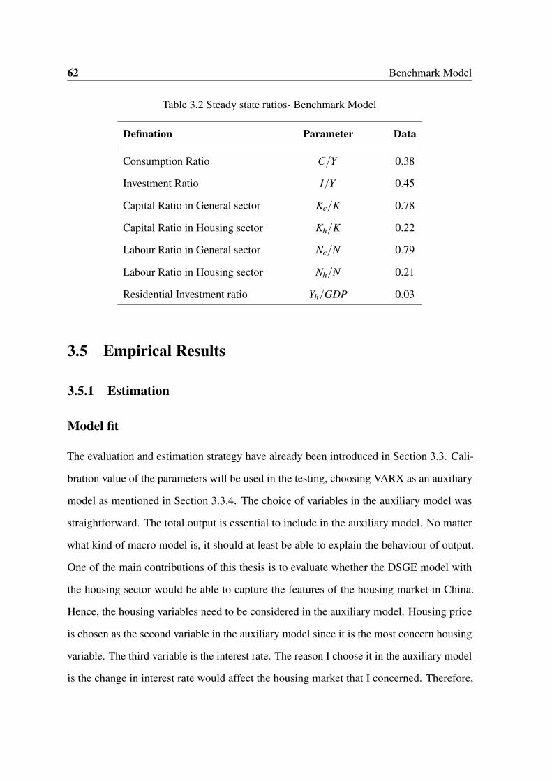
62 Benchmark Model
Table 3.2 Steady state ratios- Benchmark Model
Defination Parameter Data
Consumption Ratio C/Y 0.38
Investment Ratio I/Y 0.45
Capital Ratio in General sector Kc/K 0.78
Capital Ratio in Housing sector Kh/K 0.22
Labour Ratio in General sector Nc/N 0.79
Labour Ratio in Housing sector Nh/N 0.21
Residential Investment ratio Yh/GDP 0.03
3.5 Empirical Results
3.5.1 Estimation
Model fit
The evaluation and estimation strategy have already been introduced in Section 3.3. Cali-
bration value of the parameters will be used in the testing, choosing VARX as an auxiliary
model as mentioned in Section 3.3.4. The choice of variables in the auxiliary model was
straightforward. The total output is essential to include in the auxiliary model. No matter
what kind of macro model is, it should at least be able to explain the behaviour of output.
One of the main contributions of this thesis is to evaluate whether the DSGE model with
the housing sector would be able to capture the features of the housing market in China.
Hence, the housing variables need to be considered in the auxiliary model. Housing price
is chosen as the second variable in the auxiliary model since it is the most concern housing
variable. The third variable is the interest rate. The reason I choose it in the auxiliary model
is the change in interest rate would affect the housing market that I concerned. Therefore,

3.5 Empirical Results 63
the three variables used in the auxiliary model are: GDP, housing price and interest rate. If
the model does not pass the test, the calibrated value can be predefined as starting value to
implement Indirect Inference estimation. Hence, in this section, I am going to discuss the
Indirect Inference empirical results. Table 3.3 shows the model coefficients of calibration
and estimation together with the testing results that presented in the form of transformed
Wald and P value.
In terms of evaluation, the testing results show in the bottom of Table 3.3, which represents
that the structural model with the calibrated parameters cannot explain the data behaviour.
More specifically, the Transformed Wald statistic for variables GDP, housing price and the
interest rate is 7.41 that greater than the critical value 1.645. Also, the P-value is 0 when
the model employs calibration value, which shows that the model is severely rejected. This
indicates that the structural model does not perform well in generating the observed data
using calibrated parameters. The reason might be either the unreasonable values for some
parameters or the failure of the structural model. Therefore, it is necessary to search for
the numerical parameter values that minimise the Wald statistic and then test the model on
these values. This is why Indirect Inference estimation is employed. The bottom of the last
column in Table 3.3 shows the transformed Wald statistic of the estimated coefficients. The
results show that the estimated model using Indirect Inference method can fit the data well
according to the transformed Wald 1.02 comparing with the critical transformed Wald of
1.645. The p-value of 0.11 also verifies the finding.
In terms of estimated results, the last column in Table 3.3 provides the best fit of coeffi-
cients values. It should be noticed that all coefficients are allowed to change except quarterly
household’s discount factor (β ), the depreciation rate of capital and housing (δk, δh) since
other information are used to identify them.
All of these coefficients have moved within the 40% interval of the initial calibration
value. On the household side, the estimated elasticity of substitution of normal goods

64 Benchmark Model
consumption (σc) has jumped to 2.65. The higher value of σc implies the lower intertemporal
in general sector, which means the consumption is relatively insensitive to the change in the
real interest rate compared with the calibration value. In the housing sector, the elasticity of
substitution of housing goods consumption (σh) decreases to 0.73 , implying that the housing
consumption growth is much more sensitive to changes in the real interest rate than that in
calibration. These estimated elasticity coefficients are in line with the assumption, which the
consumption is very insensitive in the general sector and sensitive in the housing sector to the
change in the real interest rate in China. The estimated coefficient of the inverse elasticity of
labour supply (η) is 0.41 lower than its calibrated value of 0.5, which implies the elasticity
of labour supply is around 2.5. This makes the labour supply more elastic comparing with
the calibration value, which implies that the workers in China are more willing to smooth
working hours when the wage rate change.
On the firm side, the price stickiness ω adjusts to 0.52 after estimation, lower than the
calibration value. That implies the data suggest a lower degree of nominal rigidity in China,
which shows short durations (around two quarters) between price changes. This estimation
result is similar to the finding in Liu and Ou (2017) who provide the estimated price rigidity
ω=0.41. The value of the share of capital in production is significantly higher than what
was initially thought, a value of 0.66 is much closer to Zhang (2009) in their work. For
the capital demand coefficients, the coefficients k11 is lower than the starting value of 0.51,
which implies lower adjustment cost. The higher value of estimated k12 in the housing sector
implies that a lower discount rate of capital. The estimated coefficients in the capital demand
equation satisfy that the sum of k11, k12 and k13 is equal to 1.
For Taylor rule, monetary policy is estimated to be more responsive to inflation and
output fluctuation. More specifically, the inflation response θπ increase from 1.5 to 1.88,
which satisfies the Taylor principle. That implies when interest rate change one unit, the
reaction of inflation will be greater than one-for-one.

3.5 Empirical Results 65
Table 3.3 Model Coefficients: 2000Q1-2014Q4
Defination Parameter Calibration Estimation
Households:
Elasticity of substitution of consumption σc 2 2.65
Elasticity of substitution of consumption σh 1 0.73
Inverse of elasticity of labour η 0.5 0.41
Household’s discount factor β 0.985 0.985
Firms:
Price rigidity ω 0.84 0.52
Output elasticity of capital α 0.3 0.66
Quarterly depreciation rate of housing δh 0.015 0.015
Quarterly depreciation rate of capital δk 0.03 0.03
Capital demand coefficients k11, k12 0.51, 0.47 0.30, 0.69
Capital demand coefficients k13, k14 0.02, 0.25 0.01, 0.37
Capital demand coefficients k15 0.5 0.86
Monetary Policy:
Taylor Rule response to inflation θπ 1.5 1.88
Taylor Rule response to output θGDP 0.125 0.25
Trans-Wald (GDP, HP, R) 7.41 1.02
P-value 0.00 0.11
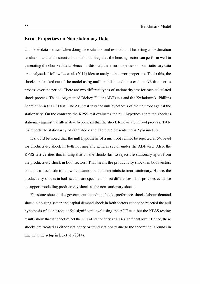
66 Benchmark Model
Error Properties on Non-stationary Data
Unfiltered data are used when doing the evaluation and estimation. The testing and estimation
results show that the structural model that integrates the housing sector can perform well in
generating the observed data. Hence, in this part, the error properties on non-stationary data
are analysed. I follow Le et al. (2014) idea to analyse the error properties. To do this, the
shocks are backed out of the model using unfiltered data and fit to each an AR time-series
process over the period. There are two different types of stationarity test for each calculated
shock process. That is Augmented Dickey-Fuller (ADF) test and the Kwiatkowski Phillips
Schmidt Shin (KPSS) test. The ADF test tests the null hypothesis of the unit root against the
stationarity. On the contrary, the KPSS test evaluates the null hypothesis that the shock is
stationary against the alternative hypothesis that the shock follows a unit root process. Table
3.4 reports the stationarity of each shock and Table 3.5 presents the AR parameters.
It should be noted that the null hypothesis of a unit root cannot be rejected at 5% level
for productivity shock in both housing and general sector under the ADF test. Also, the
KPSS test verifies this finding that all the shocks fail to reject the stationary apart from
the productivity shock in both sectors. That means the productivity shocks in both sectors
contains a stochastic trend, which cannot be the deterministic trend stationary. Hence, the
productivity shocks in both sectors are specified in first differences. This provides evidence
to support modelling productivity shock as the non-stationary shock.
For some shocks like government spending shock, preference shock, labour demand
shock in housing sector and capital demand shock in both sectors cannot be rejected the null
hypothesis of a unit root at 5% significant level using the ADF test, but the KPSS testing
results show that it cannot reject the null of stationarity at 10% significant level. Hence, these
shocks are treated as either stationary or trend stationary due to the theoretical grounds in
line with the setup in Le et al. (2014).

3.5 Empirical Results 67
For labour supply shock, housing demand shock, monetary policy shock and labour
demand in general sector no matter the P-value from the ADF test or the statistics from the
KPSS test all imply that these shocks processes are stationary. In the previous literature,
some works using different specification for the exogenous processes. For example, Smets
and Wouters (2007) employ an ARMA mark-up shock to help to fit the model well and also a
higher-order autoregressive process used as the government spending shock in Del Negro and
Schorfheide (2009). In my research, apart from the productivity shocks in different sectors,
the other exogenous shocks processes follow AR(1) dynamics or AR(1) dynamics with a
deterministic trend. The AR coefficients are determined by the estimation process, which
also can be found in Table 3.5. Most of the exogenous process are highly persistence.
Fig. 3.4 Structure Shocks

68 Benchmark Model
Table 3.4 Stationarity of Residual
Shocks ADF p-value KPSS Statistic Conclusion
Government spending 0.4593 0.238410 Trend Stationary
Preference 0.1980 0.195231 Trend Stationary
Labour supply 0.0497** 0.180101 Trend Stationary
TFP – General sector 0.9993 0.955905*** Nonstationary
TFP – Housing sector 0.7184 0.885958*** Nonstationary
Housing Demand 0.0246** 0.120453 Stationary
Monetary policy 0.0327** 0.061916 Stationary
Labour demand - General 0.0451** 0.213222 Trend Stationary
Labour demand - Housing 0.1381 0.236403 Trend Stationary
Capital demand - General 0.1401 0.209563 Trend Stationary
Capital demand - Housing 0.1801 0.179087 Trend Stationary
Notes:1. p-value with ** rejects the unit root process at 5%2. KPSS with ** (***) rejects stationarity at 5% (1%)
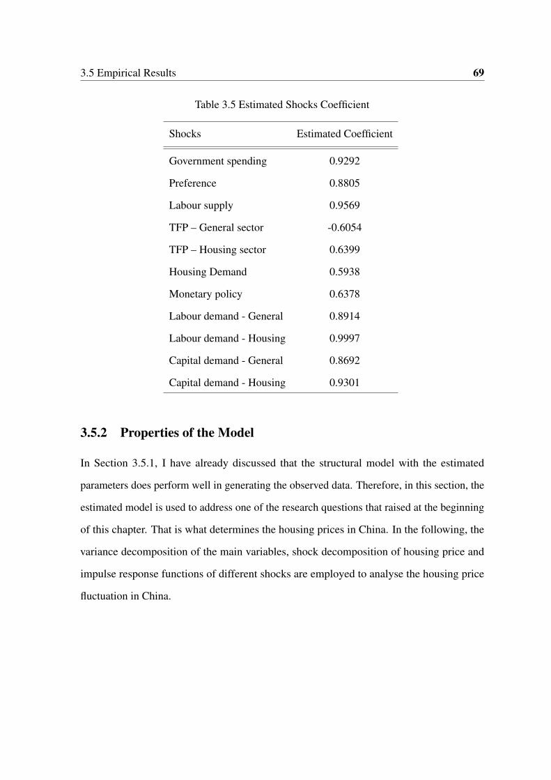
3.5 Empirical Results 69
Table 3.5 Estimated Shocks Coefficient
Shocks Estimated Coefficient
Government spending 0.9292
Preference 0.8805
Labour supply 0.9569
TFP – General sector -0.6054
TFP – Housing sector 0.6399
Housing Demand 0.5938
Monetary policy 0.6378
Labour demand - General 0.8914
Labour demand - Housing 0.9997
Capital demand - General 0.8692
Capital demand - Housing 0.9301
3.5.2 Properties of the Model
In Section 3.5.1, I have already discussed that the structural model with the estimated
parameters does perform well in generating the observed data. Therefore, in this section, the
estimated model is used to address one of the research questions that raised at the beginning
of this chapter. That is what determines the housing prices in China. In the following, the
variance decomposition of the main variables, shock decomposition of housing price and
impulse response functions of different shocks are employed to analyse the housing price
fluctuation in China.

70 Benchmark Model
Variance Decomposition
Variance decomposition of forecast errors investigates how much of the forecast error variance
of each of the variables can be explained by exogenous shocks to the other variables. Table 3.6
reports the variance decomposition of forecast errors of total output, inflation, consumption,
housing price and the interest rate at different horizons using estimated coefficients.
In terms of housing price, in the short run (1 year), the dominant driving force of housing
price fluctuations is capital demand shock in the housing sector, which explain 65.59% of
the variance in housing price. The housing demand shock also contributes to the volatility of
housing price, which accounts for 18%. By contrast, monetary policy shock only accounts
for 9.90% in the short run. In the long run (10 years), the influence of capital demand shock
and housing demand shock decrease, which the former explains 51.65% while the latter
explains only 10.32%. By contrast, the influence of technology shock in the general sector
on housing price increase, which accounts for 21.26%
As mentioned previously, the capital demand shock in housing sector captures the
regulation on firms’ use of capital. That implies the change in regulation on supply side related
to capital usage affects the housing price dramatically. Chinese housing market experiences
substantial reforms starting in 1998, the full marketisation reform promoted the privatisation
of housing. A series of regulation changes on the supply side are plausible sources of capital
demand shock. Houses were treated as welfare before reform, which the Chinese government
control the housing construction. There is no housing market at that time. However, after
reform, houses were treated as a commodity at prices determined by the market, which can be
purchased or rented. In order to boost housing market development, a series of reforms were
established on the supply side when housing has been commodified, which develop some
new regime of capital accumulation such as expanding production capacity and attracting
foreign investment in economic development. This reform witnessed the Chinese housing
market boom and the Chinese housing industry have become a pillar industry in the Chinese

3.5 Empirical Results 71
economy. According to Wu (2015), he believed that capital accumulation is a causative
factor in the growth of the housing market. The change in capital accumulation is linked
with related regulation changes8. These regulations on the supply side played a key role in
housing development.
For the real consumption, the variance decomposition shows that intertemporal preference
shock and technology shock in the general sector play a significant major role. The volatility
of real consumption is mainly driven by intertemporal preference shock. The shock explains
47.74% of the variance in real consumption in the short run (1-year forecast horizons) and
explains 13.49% in the long run (10-year forecast horizons). Technology shock in the
general sector also contributes significantly and explains 22.06% of the variance in real
consumption in the short run. However, in the long run, technology shock in the general
sector becomes more important and explains 68%. The reason why the preference shocks
play an important role in explaining the real consumption in the short run due to the inter-
temporal Euler equation, which directly affects the real consumption. We know from the
model that the productivity technology shock is the non-stationary shock, which implies
it has a permanent effect on output, consumption, capital and investment. Therefore, this
explains why productivity shock contributes significantly to explaining real consumption in
the long run.
The following variables in Table 3.6 GDP, inflation, and interest rate are non-housing
variables. The demand shock (housing preference) in the housing market plays a role in
driving the cyclical fluctuations, which account for over 10% of most variables in the short
run. The supply shock (housing technology), however, plays a minor role in driving the
cyclical fluctuations, which accounts for less than 5% of most variables. However, The
contribution of productivity shock in the general sector to the fluctuations in non-housing
variables is more important especially for the most non-housing variable. Technology shock
explains 37.87% of the variances in GDP in short tun and about 67.66% in the long run.
8Regulation change such as economic decentralisation, fiscal reform etc.
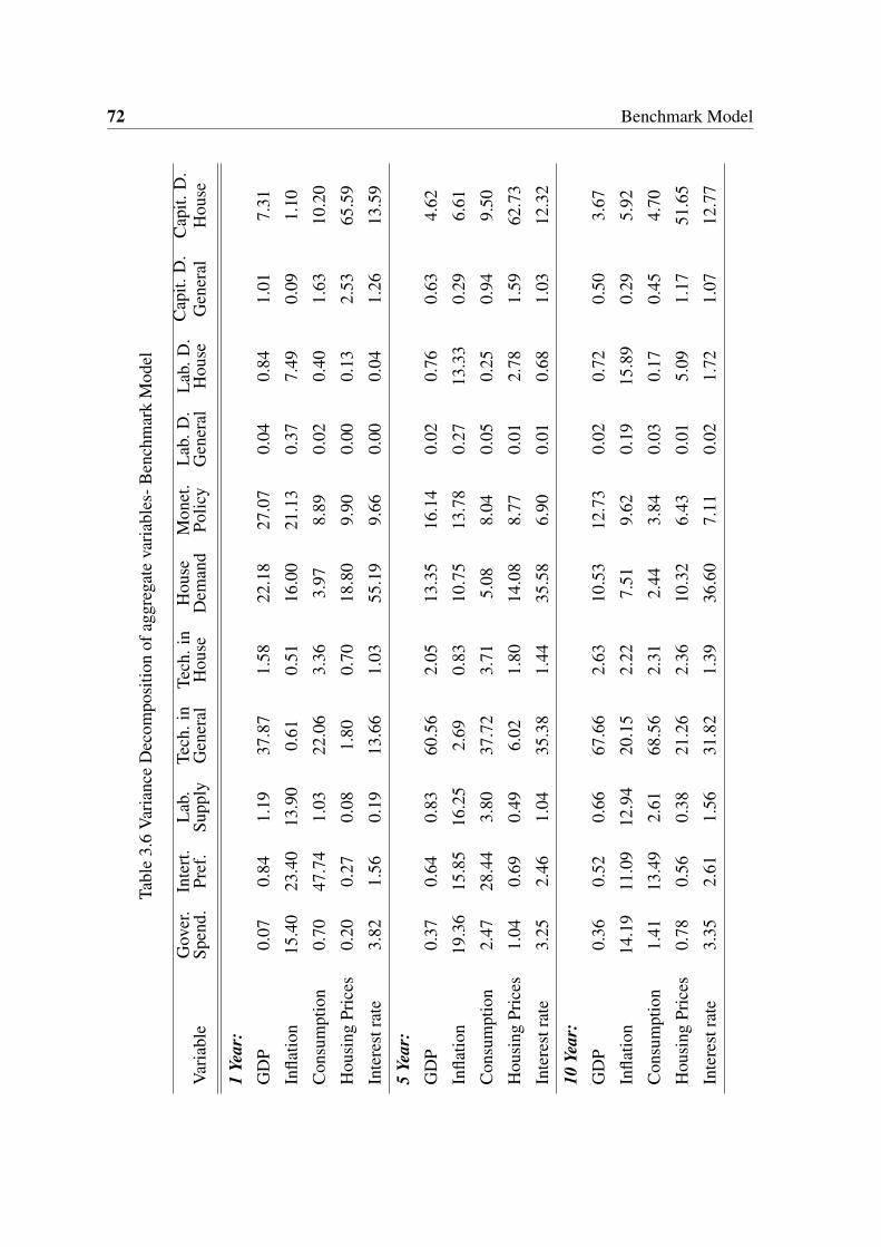
72 Benchmark Model
Tabl
e3.
6V
aria
nce
Dec
ompo
sitio
nof
aggr
egat
eva
riab
les-
Ben
chm
ark
Mod
el
Var
iabl
eG
over
.Sp
end.
Inte
rt.
Pref
.L
ab.
Supp
lyTe
ch.i
nG
ener
alTe
ch.i
nH
ouse
Hou
seD
eman
dM
onet
.Po
licy
Lab
.D.
Gen
eral
Lab
.D.
Hou
seC
apit.
D.
Gen
eral
Cap
it.D
.H
ouse
1Ye
ar:
GD
P0.
070.
841.
1937
.87
1.58
22.1
827
.07
0.04
0.84
1.01
7.31
Infla
tion
15.4
023
.40
13.9
00.
610.
5116
.00
21.1
30.
377.
490.
091.
10
Con
sum
ptio
n0.
7047
.74
1.03
22.0
63.
363.
978.
890.
020.
401.
6310
.20
Hou
sing
Pric
es0.
200.
270.
081.
800.
7018
.80
9.90
0.00
0.13
2.53
65.5
9
Inte
rest
rate
3.82
1.56
0.19
13.6
61.
0355
.19
9.66
0.00
0.04
1.26
13.5
9
5Ye
ar:
GD
P0.
370.
640.
8360
.56
2.05
13.3
516
.14
0.02
0.76
0.63
4.62
Infla
tion
19.3
615
.85
16.2
52.
690.
8310
.75
13.7
80.
2713
.33
0.29
6.61
Con
sum
ptio
n2.
4728
.44
3.80
37.7
23.
715.
088.
040.
050.
250.
949.
50
Hou
sing
Pric
es1.
040.
690.
496.
021.
8014
.08
8.77
0.01
2.78
1.59
62.7
3
Inte
rest
rate
3.25
2.46
1.04
35.3
81.
4435
.58
6.90
0.01
0.68
1.03
12.3
2
10Ye
ar:
GD
P0.
360.
520.
6667
.66
2.63
10.5
312
.73
0.02
0.72
0.50
3.67
Infla
tion
14.1
911
.09
12.9
420
.15
2.22
7.51
9.62
0.19
15.8
90.
295.
92
Con
sum
ptio
n1.
4113
.49
2.61
68.5
62.
312.
443.
840.
030.
170.
454.
70
Hou
sing
Pric
es0.
780.
560.
3821
.26
2.36
10.3
26.
430.
015.
091.
1751
.65
Inte
rest
rate
3.35
2.61
1.56
31.8
21.
3936
.60
7.11
0.02
1.72
1.07
12.7
7

3.5 Empirical Results 73
Historical Decompositions
The historical decomposition measures the contribution of each shock to the volatility of
variables over a certain sample period. Figure 3.5 decompose the real housing price over the
shocks during 2000Q1 to 2013Q4. There are some common features when decomposing the
real housing price comparing with those of the forecast error variance decompositions.
In order to make the figure clear, I classify these 11 shocks (government spending shock,
preference shock, housing demand shock, labour supply shock, productivity shock in both
housing and general sectors, capital demand as well as labour demand in both sectors and
monetary policy shock) into 6 categories. The preference shock and labour supply shock
belong to private shocks. The public shocks contain labour demand shock in different sectors
and capital demand shock in the general sector and housing sector. The policy shocks consist
of monetary policy shock and government spending shock. The total factor productivity
(TFP) include the technology shock in two sectors. The housing demand shock does not
classify into private shocks category as I want to observe how this shock influence the real
housing price.
From Figure 3.5, I find that the fluctuation of housing price is mainly driven by the
technology shock, public shocks as well as housing demand shock, which in line with
the finding in the variance decomposition. As can be seen in Figure 3.5, the housing
price experienced a sharp increase at the middle of 2005 and public shock made a major
contribution to the surge in the real housing price. An explanation of this sharp increase
is the abolishment of welfare housing provision and adoption of a more radically market-
oriented approach to housing provision at the beginning of 2005. Housing commodification
accelerates the development of housing industries, that implies more capital are needed.
The injection of capital has to lead to a new housing market cycle, which in line with Wu
(2015). It also supports the finding in variance decomposition that capital demand shock is
the main driving force of the fluctuation of real housing price. A series of housing tightening

74 Benchmark Model
policies were issued to slow down the housing price increase at starting from 2006. These
policies affect the sharp increase in the real housing price but the housing market did not
experience a sharp downturn before the global financial crisis. Hence, households needed to
think carefully about housing purchase. However, the housing boom was hit hardest in late
2007. The outflow of capital caused by the boom of the stock market in 2007. Households
engaged in the stock market. Hence, the demand of housing decrease. In the following, the
housing market also hit by the global economic crisis in 2008. One of the approaches that
the central government attempt to stimulate economic growth after the crisis is using housing
industries as a booster. The stimulation package includes investment in the housing market,
a reduction in interest rates and enhancing capital liquidity. Some new regimes of capital
accumulation such as expanding production capacity and attracting foreign investment were
launched to encourage the housing market. According to Wu (2015), the minimum capital
requirement for commodity housing projects was reduced from 30% to 20%. This is shown
clearly from the graph, in which the rapid rebound following the temporary slowdown. After
2010, the housing price started to fall down. A series of property purchases restrictions and
low productivity, I believe, is the main culprit.
Fig. 3.5 Shock Decomposition - Real Housing Price

3.5 Empirical Results 75
Impulse Response Functions
Impulse response functions obtained from the estimated model are shown in this section.
There are three main shocks I concern about: housing demand shock, monetary policy shock
and technology shock in the general sector. In order to study the reaction to these shocks
in different sectors, in the first row I report the response of main model variables in the
general sector and the response of main model variables in the housing sector are shown in
the second row. The third row shows the total GDP and interest rate. The other shocks can
be found in Appendix B
The effects of housing demand shock
Figure 3.6 shows how these key macro variables behave in different sectors when there is
a positive housing demand shock (15.5 standard error). It is assumed that the shocks εht
following the exogenous process lnεht = ρh lnεh
t−1 + vh,t . I focus on the housing sector first.
A positive housing demand shock leads to a significant increase in housing demand, which
lead to the increments in housing price. Supply of housing also rises to meet the high demand
for housing. The housing boom not only affect the housing sector, but the general sector
is also been affected. The housing boom leads to the expansion of output in the general
sector and inflation, which slightly increase compared to those in the housing sector. And a
subsequent increase in interest rate. The impulse responses of selected variables to housing
demand shock are in line with the main findings in many previous literature.
As mentioned in the model part, housing demand shock can be think as the change of
preferences on housing due to social, institutional or income changes. The housing institution
reforms can be explained as the important institutional changes. The private housing market
was established after a series of reforms. A series of reforms were launched, and the welfare-
oriented housing provision was abolished. These lead to the increments in housing demand.
In order to meet the extra demand, the supply of housing raised. Overall, the housing

76 Benchmark Model
Fig. 3.6 Impulse responses to Housing Demand Shock
reform stimulate the whole economic growth, which is a significant fundamental economic
change. On the other hand, China has experienced economic transformation involving fast
productivity progress. According to Bian and Gete (2015), the higher income the household
obtain benefit from higher productivity, the higher demand for housing they desire.
The effects of the monetary policy shock
Figure 3.7 plots impulse responses to the monetary policy shock (0.45 standard error) to
the economy. A positive shock to the monetary policy decrease all the variables in different
sectors. The standard interest rate channel of monetary policy transmission show that such
monetary contraction discourages the investment and consumption so that decrease the total
output. The decrease of consumption shifts the pressure through changes in inflation, which
lower the inflation as well as housing price. That means a tightening of monetary policy
can have a drop in housing price. This maybe due to the Taylor Rule in the model affect
the consumption through Euler equation. This leads to influence the demand of housing,

3.5 Empirical Results 77
Fig. 3.7 Impulse responses to Monetary Policy Shock
which triggers the housing price. These results are consistent with the main finding of many
previous literature. A tightening of monetary policy shock decreases all components of real
aggregate demand and real housing prices.
The effects of technology shocks in the general sector
Figure 3.8 plots the impulse responses of model variables to a 3.20 standard error total
factor productivity shock. It should be noticed that the productivity shock in both sectors
follow a unit root process. This non-stationary process has the permanent effect on some
macroeconomic variables such as total output, output in different sectors, real consumption,
housing demand and the stock of physical capital. These variables become more persistent
afterwards lasting over 40 quarters. In response to a positive productivity shock in the
general sector, the supply of output in the general sector goes up due to superior technology.
The increase in supplying lead to the decrease in inflation. The interest rate decrease as a
results of falling inflation. In the housing sector, we can see that the increase of housing

78 Benchmark Model
Fig. 3.8 Impulse responses to Technology shocks in general sector
supply decrease the housing price at the very beginning. As the demand for housing increase
significantly after period 5, the housing price pushes up at the same period.
3.6 Conclusion
The aim of this chapter is focusing on answering the first research question: What is the
driving force in the fluctuations of housing price. The estimated DSGE model with explicit
modelling of the price and quantity of the housing sector and non-stationary productivity
shock is used to study housing market fluctuations in China. Indirect Inference method
is employed to find a right model to explain the data behaviour in the Chinese housing
market. The testing results show that the model using the calibration value is rejected by the
data. Hence, the Indirect Inference method is used to estimate the model over the period
2000-2014, which find out a set of coefficients that can past the test. The model can fit the
data well when a variety of endogenous variables are added to the auxiliary model, explaining
the output, housing price and interest rate that I concerned about. Once find the right model

3.6 Conclusion 79
that can perform well in explaining the data, I discover the housing market using this model.
In terms of the driving force of fluctuations in the Chinese housing market, the variance and
shock decomposition suggest that the capital demand shock plays a significant major role in
explaining the housing price. That maybe because the housing market reform stimulates the
Chinese housing industry, which develops some new regime of capital accumulation. These
regulation change on the supply side played a key role in housing development.


Chapter 4
Model with Collateral Constraint
4.1 Introduction
In the last chapter, I have established a benchmark model with a rich set of shocks to explain
the behaviours and the sources of fluctuations in the Chinese housing market using Indirect
Inference method. The testing results show that the estimated benchmark model can fit
the Chinese data well on the one hand, and that encompasses most of the views on the
sources and propagation mechanism of business cycles on the other hand. The increasing
interest in the DSGE housing model literature have focused on the collateral constraint
on the households’ side, which treats as a channel that connects the housing market to
the wider economy. Previous studies emphasise the role play as the housing collateral in
the households’ optimal decision. They add the channel by splitting the households into
two types: patient (lenders) and impatient (borrowers). The impatient households in the
economy face a binding collateral constraint when participating in loan and mortgage market.
Therefore, the collateral constraint is a channel to amplify the collateral effect on households
borrowing to the whole economy.
One important work is that Iacoviello and Neri (2010) present a Bayesian estimated
DSGE model to study the housing market and business cycle, which emphasise the spillovers

82 Model with Collateral Constraint
effect from the housing market to the wider economy by adding the collateral constraint on
the households’ side. There are different ways to quantify housing market spillovers. The
Iacoviello type model focus on one aspect of spillovers, that is, the relationship between
housing wealth and non-housing consumption. Inspired by Kiyotaki and Moore (1997), these
Iacoviello type model feature a collateral constraint on the households side. That implies
the borrowing capacity of impatient households is limited by a fraction of the expected
present value of total assets such as houses, lands and capitals. In their model, the borrowing
constraint can be thought as a channel to connect the housing market and the rest of the
economy, allowing for ’spillover’ from one sector to the other through that channel.
Iacoviello (2005) constructs a DSGE model including collateral constraints tied to real
estate values for the impatient households. In the extended model, both firms and impatient
households face the credit constraint. The model is used to explain both the business cycle
facts and the interaction between asset prices and economic activity. Then, Iacoviello and
Neri (2010) extend the work of Iacoviello (2005) and present a Bayesian estimated DSGE
model. They show that collateral effects on households borrowing amplify the response
of non-housing consumption to given changes in fundamentals, thus alter the propagation
mechanism.
The transmission mechanism of collateral constraint in Iacoviello type model work as
following. When there is a positive demand shock, the demand for housing rise, housing
price also increases. The rise in asset prices increases the borrowing capacity of the debtors.
That implies they can borrow more due to the high asset prices, allowing them to spend
and invest more. The change in investment will cause the output to fluctuate, which in turn
influences the current asset price. Therefore, a significant transmission channel is generated
through the dynamic interaction between the credit constraint and asset prices.
Based on their analysis framework, more types of shocks and frictions are introduced
to study the housing market. Ng (2015) employ Iacoviello type model to study the sources

4.1 Introduction 83
and consequences of the fluctuations in the Chinese housing market. In terms of the nature
of shocks driving housing price dynamic, they find that housing demand shock explains the
majority of the fluctuations in housing price. In terms of spillover effect work through the
collateral constraint, there is not a unique way to quantify the effect, which depends on the
nature of shocks. Housing demand shock has a larger contribution to the spillover effect
compared to the technology shock. However, the technology shock plays a negligible role in
the spillover effect. Liu and Ou (2017) also use a DSGE model with a collateral constraint
to study the Chinese housing market. Apart from investigating the main driving force of
housing market fluctuation, they also study the housing market spillovers effect in China.
They find that there is a weak spillover effect from the housing market to the wide economy.
He et al. (2017) employ a Bayesian DSGE model with collateral constraints to investigate the
interaction between the housing market and the business cycle. They find that the collateral
constraint plays a significant role in explaining the fluctuate of the business cycle in China,
which amplifies the impact of various economic shocks.
While these studies have highlighted the collateral constraint on households borrowing, to
date there has been no evaluation of the general equilibrium model with collateral constraint.
This is the perspective adopted here. Indirect Inference evaluation is used to check whether
the DSGE housing model with a collateral constraint on the household side can explain the
Chinese housing market well. From the modelling point of view, my starting point is the
benchmark model that introduced in Chapter 3, which a DSGE model include the explicit
modelling of the price and quantity of the housing sector with non-stationary productivity
shock. In order to examine whether the model with collateral constraint can explain the
Chinese housing market well, I include another feature into the benchmark model. That is
collateral constraints tied to the housing values for impatient households, as in Iacoviello
and Neri (2010). This chapter tries to identify whether the Chinese housing market can be

84 Model with Collateral Constraint
explained better using a model with collateral constraint compared to the benchmark model
through Indirect Inference evaluation.
This chapter is structured as follows: the model with a collateral constraint is presented
in Section 4.2, and the collateral channel is also analysed. The estimation part is outlined in
Section 4.3, which introduce the data used in this chapter and the baseline calibration as well
as the estimation results. In this section, I will explore whether the model can perform well if
it introduces the collateral constraint. The standard analyses are shown in Section 4.4 that
including historical and variance decomposition and impulse response functions to different
shocks. Finally, I conclude the housing model with collateral constraint in Section 4.5.
4.2 Model
Impatient households are introduced to feature the collateral constraint. Therefore, there is
one more household on the demand side. Five types of agent exist in the economy: patient
households, impatient households, housing sector, general sector and central bank. The
key feature that distinguishes between patient and impatient households is the discount rate.
Impatient households discount future utilities more heavily than the patient ones due to the
heterogeneous preference. In each period, patient households consume, accumulate housing
and supply funds to impatient households. Impatient households work, consume, purchase
housing through borrowing from patient households. The firms in both sectors behave as
before, and I keep them as same as in the benchmark model.
Impatient Households
There is a continuum of measure 1 of impatient households. The representative impatient
households derive utility from consumption, housing purchase and disutility from supplying
labour. The representative impatient households expected discounted lifetime utility is given

4.2 Model 85
by
UIt = E0
∞
∑t=0
βIt
εpt
[C1−σc
It1−σc
+ εht
H1−σhIt
1−σh− ε
ltN1+η
t
1+η
](4.1)
where E0 is the expectation formed at period 0, β It is the subjective discount factor, the
impatient households obtain utility from consumption goods CIt , new housing HIt and get
disutility from labour supply Nt . The parameters σc, σh are the inverse of intertemporal
elasticity of substitution of consumption and housing, while η denotes the inverse of the
elasticity of work time with respect to real wage.There are three shocks in the utility function
like in Chapter 2. They are εpt , εh
t and ε lt respectively. ε
pt and ε l
t are shown here to express
intertemporal preferences shock and labour supply shock. The term εht captures shock to
housing demand 1. The impatient households’ budget constraint is
CIt + ph,t(HIt − (1−δh)HI,t−1)+(1+ rt−1)BI,t−1 = wtNt +BIt (4.2)
From equation (4.2), it can be seen that the wealth of impatient households consists of two
parts, which is shown on the right-hand side. One of the incomes comes from supplying
labour wtNt . The other comes from borrowing from patient households BIt . The left-hand
side displays the outflow of funds. The impatient households use his wealth in each period
for buying consumption goods CIt , new housing HIt with relative price ph,t and payback last
period’s debt with rt−1.
Collateral constraint
Private borrowing is subject to an endogenous limit as in Iacoviello and Neri (2010). Impa-
tient households borrow from patient households to finance their consumption and housing
purchases. The borrowers face the borrow constraint: the value they can borrow is limited by
1The detail of housing demand shock can be found in Chapter 2

86 Model with Collateral Constraint
a fraction of the expected present value of their housing asset. That is,
BIt ≤ mEt(ph,t+1HIt
1+ rt) (4.3)
where m is the loan to value ratio for impatient households. It should be noticed that the
change in the expected relative price of housing affects the ability of borrowing directly. This
collateral constraint can be treated as a channel to evaluate the transmission of monetary
policy shocks in the model. For simplicity, there is an assumption that has to hold when
finding the optimal behaviour of impatient households: the collateral constraint (4.3) is
always satisfied with equality. That means parameters are calibrated in a way to make it
bind. Therefore, in the steady state, the impatient households’ borrowing constraint is always
binding.
Impatient households’ Problem
The impatient households’ problem is choosing CIt ,Nt ,BIt and HIt to maximise their lifetime
utility (4.1) subject to (4.2) and (4.3). The Lagrangian:
L = E0
∞
∑t=0
βIt
εpt (
C1−σcIt
1−σc+ ε
ht
H1−σhIt
1−σh− ε
ltN1+η
t
1+η)
−λIt [CIt + ph,t(HIt − (1−δh)HI,t−1)+(1+ rt−1)BI,t−1 −wtNt −BIt ]
−λ′It [BIt −mEt(
ph,t+1HIt
1+ rt)]
(4.4)
The first order conditions:
CIt : C−σcIt ε
pt = λIt (4.5)
Nt : εpt ε
lt Nη
t = wtλIt (4.6)

4.2 Model 87
BIt : βItEtλI,t+1(1+ rt) = λIt −λ
′It (4.7)
HIt : λIt ph,t = εpt ε
ht H−σh
It +βIEt(λI,t+1 ph,t+1(1−δh))+λ
′Itm
Et ph,t+1
1+ rt(4.8)
The marginal utility losses of choosing relevant allocation are shown on the left-hand
sides of the above equations. On the contrary, marginal utility gains of choosing relevant
allocations are represented on the right-hand sides of the above equations. It should be
noticed that both the Euler equation (4.7) and the housing demand equation (4.8) are different
from the standard form due to the presence of λ ′It , which is the Lagrange multiplier on the
borrowing constraint. The multiplier λ ′It represents utility increase that would come from
borrowing, consuming in (4.7) or investing in (4.8).
Equation (4.5) links the borrower’s marginal utility of consumption to the Lagrangian
multiplier. Equation (4.6) is a standard labour supply equation which represents the sub-
stitution between labour supply and consumption. Equation (4.7) is impatient households’
borrowing. The left-hand side of equation (4.7) is the marginal utility loss, which is the
expected value of debt repayment of one unit of borrowing β ItEtλI,t+1(1+ rt). The right-
hand side shows the marginal utility gain, which is the utility gain comes from one unit of
additional consumption λIt , get rid of the loss of value due to the borrowing constraint, λ ′It .
A standard Euler condition is presented when λ ′It = 0 for all t in equation (4.7). Equation
(4.8) represents an intertemporal condition on housing demand, which requires the marginal
utility of current general goods consumption equal to the marginal gain of housing services.
The marginal utility gain of housing services shown on the right-hand sides of equation (4.8)
consists of three components: first, the direct utility from an additional unit of housing. The
second component is the expected utility coming from the possibility of expanding future

88 Model with Collateral Constraint
consumption relying on the realised resale value of the housing purchased in the previous
period. The third component is the marginal utility gain from the value of housing as the
collateral asset. Further imply:
Nη
t
C−σct
εlt = wt (4.9)
H−σhIt
C−σcIt
εht +β
I(1−δh)Et(ph,t+1C−σc
I,t+1
C−σcIt
εpt+1
εpt
)+(1−βI(1+rt)Et(
C−σcI,t+1
C−σcIt
εpt+1
εpt
))mEt ph,t+1
1+ rt= ph,t
(4.10)
In order to understand the behaviour of impatient households of housing purchases, I
combine the binding borrowing constraint (4.3) with the budget constraint (4.2) and obtain:
(ph,t −m
1+ rtEt ph,t+1)HIt = wtNt + ph,t(1−δh)HI,t−1 −CI,t − (1+ rt−1)BI,t−1 (4.11)
From equation (4.11), the term mEt ph,t+1/(1 + rt) represents the amount of funds
that the impatient households can borrow from the patient households. The term ph,t −
mEt ph,t+1/(1+ rt) is the instalment payment required to purchase one unit of housing. The
net worth of the impatient households in period t can be found on the right-hand side of
equation (4.11). The total worth consists of the labour income from supplying labour to
the firms plus the value of housing accumulated in the previous periods. The net worth
of the impatient households is that the total worth gets rid of the net of consumption and
debt repayment. In the long equilibrium, the impatient households use all their net worth to
finance the instalment payment that required to purchase HIt units of housing.

4.2 Model 89
Patient Households
The representative patient households derive utility from consumption and housing. In
this category of consumers, I follow Monacelli (2009) assuming that the typical patient
households are the owner of the monopolistic firms in each sector. The patient households
try to maximise lifetime utility:
Upt = E0
∞
∑t=0
βpt
εpt [
C1−σcpt
1−σc+ ε
ht
H1−σhpt
1−σh] (4.12)
where the variables in (4.12) share the similar interpretations in equation (4.1). The key
feature that distinguishes the patient and impatient households’ behaviour is the discount
factor. In equilibrium, the patient households lend to the impatient households with borrowing
constraint binding in the steady state. I assume that patient households are more patient than
impatient households, implying
βpt ≥ β
It (4.13)
The patient’s sequence of budget constraints reads:
Cpt + ph,t(Hpt − (1−δh)Hp,t−1)+St = (1+ rt−1)St−1 +π (4.14)
The right-hand side of equation (4.14) represents the total wealth of patient households,
which consists of gross returns from lending and the profits from the holding of monopolistic
competitive firms. The left-hand side of equation (4.14) is the outflow of funds of the
patient households, which contain consumption, housing purchase and lending. Following
Monacelli (2009), there are two reasons to disregard the labour supply choice by the patients’
households. First, for simplicity, I disregard for labour supply of patient households making
the level of output independent of the relative labour share of the two households. Second,
the patient households are more patient than impatient households, which prefer to hold their

90 Model with Collateral Constraint
wealth obtain from lending funds and from owning firms in different sectors. Hence, they
will end up owning all assets and choose to work very little in the steady state.
Patient households’ Problem
The patient households try to maximise a lifetime utility function (4.12) subject to the budget
constraint (4.14) through Lagrangian:
L =E0
∞
∑t=0
βpt
εpt (
C1−σcpt
1−σc+ε
ht
H1−σht
1−σh)−λpt [Cpt + ph,t(Hpt −(1−δh)Hp,t−1)+St −(1+rt−1)St−1−π]
(4.15)
The first order conditions:
Cpt : C−σcpt ε
pt = λpt (4.16)
St : λpt = βptEtλp,t+1(1+ rt) (4.17)
Hpt : λpt ph,t = εpt ε
ht H−σh
pt +βpEt(λp,t+1 ph,t+1(1−δh)) (4.18)
Again, in the above equations, the marginal utility losses of choosing relevant allocations
is shown on the left-hand sides; the marginal utility gains of choosing relevant allocations
is presented on the right-hand sides. For housing demand of patient households (4.18), the
marginal utility gain only depends on two components compared to the housing demand of
impatient households. That is the direct utility gain of an additional unit of housing and the
expected utility coming from the future consumption. Further imply:
C−σcpt ε
pt = β
pEtC−σcp,t+1ε
pt+1(1+ rt) (4.19)

4.2 Model 91
εht H−σh
pt =C−σcpt ph,t −β
pEt(C−σcp,t+1 ph,t+1(1−δh)
εpt+1
εpt
) (4.20)

92 Model with Collateral Constraint
4.3 Estimation
4.3.1 Data
The collateral constraint is introduced in the benchmark model by splitting the households
into two types (patient households and impatient households). Therefore, five more variables
involved in this model. They are consumption of patient households (Cpt), consumption of
impatient households (CIt), housing demand of patient households (Hpt), housing demand of
impatient households (HIt) and impatient households borrowing (BIt). The rest variables are
the same as that used in Chapter 3, which sample period covers from 2001Q1 to 2014Q4.
The detail of data description are outlined in the Appendix A. It should be noticed that the
unfiltered data also used in this chapter to do the evaluation and estimation.
4.3.2 Calibration
Calibrated parameter values are introduced in this section, which are divided into two groups
like in Chapter 3. The parameter values in the first group govern the dynamics of the model,
which are calibrated according to previous literature and the observations in some empirical
analyses. If the model using these calibrated values cannot pass the test, I would reestimate
these parameters using Indirect Inference estimation. The calibration values in this group
keep as same as those in Chapter 3 except for β p, β I , m. These three more parameters are
introduced since the collateral constraint is employed in this chapter. The second group of
the parameters are the steady state of the model, which are obtained from the data same in
those in Chapter 3.
In this chapter, I split out the households into two types (patient households and impatient
households) and introduce the collateral constraint between these two households. The key
feature that distinguishes between patient and impatient households is they have the different
discount factor. The discount factor of impatient households is less than the discount factor of

4.3 Estimation 93
patient households, which implies the patient households are more patient than the impatient
households. Hence, these two parameters are calibrated to evaluate and estimate. They are
the discount factor of patient households β p, the discount factor of impatient households β I .
Because of lending between two different households, one more parameter is introduced.
That is loan-to-value ratio m.
In terms of the discount factor, I calibrate β p at 0.985 and β I at 0.97 in line with Iacoviello
and Neri (2010) to guarantees that the borrowing constraint is binding for the impatient
households in equilibrium. The binding constraint captures the financial accelerator effect,
which allows the interaction between the housing sector and the rest of the economy.
m is the loan-to-value ratio, which captures the amount of loan that impatient households
can get with a given market value of the house. The maximum loan-to-value ratio in China is
0.8. However, the average loan-to-value ratio is much lower than that, around 0.3 to 0.42.
According to Liu and Ou (2017), the observed debt-to-GDP ratios of households is around
23%. Hence, I calibrate the loan-to-value ratio at 0.3, which captures the features of the
Chinese economy.
2The data are from Housing Finance Network.

94 Model with Collateral Constraint
Table 4.1 Calibrated Coefficients - Model with Collateral Constraint
Defination Parameter Calibration
Households:
Elasticity of substitution of normal goods consumption σc 2
Elasticity of substitution of housing goods consumption σh 1
Inverse of elasticity of labour η 0.5
Patient households’ discount factor β p 0.985
Impatient households’ discount factor β I 0.97
Loan-to-value ratio m 0.3
Firms:
Price rigidity ω 0.84
Output elasticity of capital α 0.3
Quarterly depreciation rate of housing δh 0.015
Quarterly depreciation rate of capital δk 0.03
Capital demand coefficients k11, k12 0.51, 0.47
Capital demand coefficients k13, k14 0.02, 0.25
Capital demand coefficients k15 0.5
Monetary Policy:
Taylor Rule response to inflation θπ 1.5
Taylor Rule response to output θGDP 0.125

4.3 Estimation 95
4.3.3 Empirical Results
In this section, I am going to discuss the Indirect Inference empirical results. The VARX
auxiliary model is still used in the evaluation and estimation in this chapter. The choice
of the auxiliary model is in line with the model in Chapter 3, which include total output,
housing price and nominal interest rate in the auxiliary model. I do the evaluation first. If
the model does not pass the test, the calibrated value can be predefined as starting value to
implement Indirect Inference estimation. It should be noticed that all the coefficients are
allowed to change when doing the estimation except for quarterly discount rate of patient
and impatient households (β p,β I), quarterly depreciation rate of capital and housing (δk,δh)
and the loan-to-value ratio (m) because they are identified through accounting information
or other government policy. The simulated annealing algorithm is used when applying
Indirect Inference estimation to discover the best fit set of coefficients. Table 4.2 presents
the empirical results for the model with collateral constraint. The calibration values are also
shown here for comparison.
I compare the estimated values with the calibrated values. The results show that all of
these estimated values have moved some way from the initial calibration values. On the
households side, for the estimated elasticity of substitution of consumption and housing, σc
is estimated to be 3.30 and σh has increased to 2.55, both estimated values are larger than the
initial values. The higher value of σi means that the consumption growth is less sensitive to
changes in the real interest rate. From the estimated results, the estimated σh is still lower
than the estimated σc, which implies that the substitution of housing goods is still relatively
more sensitive compared to the substitution of general consumption goods when changing in
the real interest rate. The estimated inverse of elasticity of labour supply η is significantly
larger than the starting value, which implies that labour supply inelastic. However, this high
inverse of elasticity of labour supply is much closer to other research reported by Zhang
(2009) who employed the DSGE model to study Chinese monetary policy.

96 Model with Collateral Constraint
On the firm side, for nominal rigidities parameters, the price stickiness ω is estimated
to be 0.33, much lower than the calibration value. The parameter ω measure the degree of
nominal rigidity. The estimated result shows that only around 33% of all firms cannot adjust
their price while the remaining 67% can adjust. This implies that the Chinese economy may
not be that sticky, which is similar to the empirical results in Liu and Ou (2017).
The value of the share of capital in production adjusts slightly, which only increase to
0.31. For capital demand coefficients, the coefficient k11 is lower than the starting value.
This implies that lower adjustment cost. The higher value of estimated k12 implies that lower
discount rate of capital. The coefficients k13 remains the same as the starting value. The
long-run relationship among coefficients in the capital demand equation is also approximately
satisfied, which is that k11 + k12 + k13 = 1.
Overall, monetary policy is estimated to be less responsive to inflation and more respon-
sive to output fluctuation. More specifically, the responsiveness of interest rates to inflation
θπ increase from 1.5 to 1.2. On the contrary, the responsiveness of output increase to 0.42
compared with the calibrated value.
This chapter aims to investigate the case when there is a collateral constraint. I want to
explore whether the model can perform well if it introduces the collateral constraint. To this
end, I compare the testing results generated from the benchmark model, where there is no
lending, with those with collateral constraint. Table 4.3 represents the comparison of the
testing results based on Indirect Inference estimation of the two models. The results show
that both models can pass on the weaker test, but the model with the collateral constraint is
obviously inferior to the benchmark model according to the Wald statistic. The benchmark
model is more probable.
In order to check both models performance with the stronger test, I add one more
endogenous variable to the existing auxiliary model. The test becomes more stringent and
powerful when I extend the features of the structural model that the auxiliary model seeks

4.3 Estimation 97
to match. The second row of Table 4.3 shows the testing results when I raise the power of
the test. The results display that the only benchmark model can pass the stronger test at 3%
significance level, while the collateral model does not pass. That implies the benchmark
model is the best model using the Wald statistic as a guide.
Different model with different coefficients may give different analysing results. Therefore,
it should be cautious when choosing the model. The benchmark model is better to be chosen
when do not focus on the lending since it has the better Wald statistic. If lending is the
important part when analysing the economy, the model with collateral constraint should be
considered. In the following, I am going to do the standard analysis such as impulse response
functions, variance and historical decomposition for the model with collateral constraint.

98 Model with Collateral Constraint
Table 4.2 Estimated Coefficients - Model with Collateral Constraint
Defination Parameter Calibration Estimation
Households:
Elasticity of substitution of consumption σc 2 3.30
Elasticity of substitution of housing σh 1 2.55
Inverse of elasticity of labour η 0.5 6.96
Patient households’ discount factor β p 0.985 0.985
Impatient households’ discount factor β I 0.97 0.97
Loan-to-value ratio m 0.3 0.3
Firms:
Price rigidity ω 0.84 0.33
Output elasticity of capital α 0.3 0.31
Quarterly depreciation rate of housing δh 0.015 0.015
Quarterly depreciation rate of capital δk 0.03 0.03
Capital demand coefficients k11, k12 0.51, 0.47 0.46, 0.53
Capital demand coefficients k13, k14 0.02, 0.25 0.02, 0.14
Capital demand coefficients k15 0.5 1.33
Monetary Policy:
Taylor Rule response to inflation θπ 1.5 1.2
Taylor Rule response to output θGDP 0.125 0.42
Trans-Wald (GDP, HP, R) 22.67 1.49
P-value 0.00 0.06

4.3 Estimation 99
Table 4.3 Comparison of the Testing Results Based on II estimation
Auxiliary Model-VARX(1) Benchmark Model Collateral Model
GDP, HP, R 1.02 1.49
(0.11) (0.06)
GDP, HP, R, C 1.92 3,46
(0.03) (0.00)
4.3.4 Indirect Inference Power Test
In the last section, the Indirect Inference testing is employed to evaluate the estimated
structural model. We would like to know how powerful the Indirect Inference test is.
Therefore, in this section, I am going to check the evaluation of the power of Indirect
Inference. In order to evaluate the power of Indirect Inference test on both benchmark
model and model with collateral constraint, I follow Le et al. (2012) and Le et al. (2016) to
conduct Monte Carlo power statistical test against parameter misspecification. Following
their research, they assume the models they used is the true model and the estimated residuals
are also treated as the true residual. Then they use the result of the Monte Carlo experiment
to establish their degree of accuracy.3 They use the Monte Carlo experiment to show that
how often the test rejects at the chosen nominal rejection rate. Their results show that
the confidence level is 5.7% when the true rejection rate at a nominal 5%. Therefore, this
experiment is fairly accurate. I employ their experiment results and treat estimated benchmark
model as well as the constraint model as the true model, using the true rejection rate at a
nominal 5% with a three variables VARX(1). Now I am interested in how the frequency of
rejection of the false model when both true models deviate increasingly from the original.
310000 Monte Carlo experiments are set up to obtain the 10000 sample of data. In each sample, theinnovations were bootstrapped to find the Wald distribution.

100 Model with Collateral Constraint
The false models are created by moving the parameters away from their true values (estimated
value) by x % in both directions for alternate values.
Table 4.4 displays the rejection rates at a nominal 5% given the parameter falseness from
0.5% to 7%. 4 We can see clearly from the table that when the falsity of parameters increases,
the probability of rejecting the false model increase. This implies the power is considerably
high given a significant falseness. More specifically, the benchmark model is 100% rejected
when the falsity of parameters increases to 7%. Comparing with the benchmark model,
the model with collateral constraint seems more sensitive to the increase in the degree of
falseness. The rejection rate has already increased to 100 when the degree of falseness
equal to 3. It is interesting to find that the model with collateral constraint has more power
compared with the benchmark model. It might be because the collateral model has more
restrictions, so a small change in the parameter will create the more significant overall worse
match.
Table 4.4 Monte Carlo Power test- 3 variables VARX(1)
Parameter Falseness TRUE 0.5% 1% 1.5% 3% 3.5% 5% 7%
Benchmark Model 5 7.2 9.6 13.4 41.1 63 85.6 100
Model with collateral constraint 5 20.5 57.4 88.7 100 100 100 100
The testing results in the last section show that the benchmark model passed at 3%
significance level while the model with collateral constraint did not pass when a 4-variable
VARX(1) was used. I want to check how robust the benchmark model is with respect to
misspecification and I also want to gauge to what extent the collateral model was misspecified.
Hence, this attracts me to do the Monte Carlo experiment again, but this time, the rejection
rates at a nominal 3% with a 4-variable VAR. Table 4.5 displays that how the rejection rates
vary when one more endogenous variable is included in the auxiliary models. It is interesting
4The rejection rate is obtained using true data from the true model and false model, which calculate howmany false model would be rejected by the true data from the true model with 95% confidence.

4.3 Estimation 101
to find that increasing one more endogenous variable raise the power of Indirect Inference test
as well. In this case, the benchmark model is already 100% when the falsity of parameters
just increase to 5%. Comparing with the benchmark model, the collateral model rejects 99%
of the time when the parameter falseness only raises to 3.5%. The more features that the
auxiliary model tries to match, the higher the probability that model is rejected by the data,
which is in line with the argument.
Table 4.5 Monte Carlo Power test- 4 variables VARX(1)
Parameter Falseness TRUE 0.5% 1% 1.5% 3% 3.5% 5% 7%
Benchmark Model 3 3.7 4.9 6.6 42 82.2 100 100
Model with collateral constraint 3 6.1 7.1 8.4 65.8 99 100 100
4.3.5 Error Properties on Non-Stationary Data
In the last section, I discuss the estimation and testing results of the model with collateral
constraint. Before doing the standard analysis such as IRFs, variance and historical decom-
position, I follow Le et al. (2014) to analyse the error properties. These shocks are backed
out of the model using the non-stationary data (Figure 4.1) and fit to each an AR time series
process over the period. Table 4.6 shows the stationarity of each shock and also the estimated
AR parameters. I employ two different types of stationarity test for each calculated shock
process: Augmented Dickey- Fuller (ADF) test and Kwiatkowski Phillips Schmidt Shin
(KPSS) test.
The ADF test tests the null hypothesis that the shock follows a unit root process, against
the alternative hypothesis that the shock is stationary. The ADF testing results show in
the second column of Table 4.6, we can see from the table that the labour supply shock,
housing demand shock, capital and labour demand shock in general sector as well as the
monetary policy shock reject the unit root process at 10%, 5% and 1% significant level

102 Model with Collateral Constraint
respectively. The p-value of the rest shocks, except for productivity shock in different sectors,
show the borderline non-rejection at 10% significance. However, the p-value of productivity
shock in both sectors approximately equals to 1, which implies a strong non-rejection of
the null hypothesis. According to DeJong et al. (1992), the very low power when errors are
autoregressively correlated is one of the problems of the ADF test. That implies the testing
does not perform well when errors are autoregression. Therefore, the KPSS stationary test is
employed to re-evaluate the structural error.
In terms of the KPSS test, on the contrary, tests the null hypothesis that the shock is
stationary against the alternative hypothesis that the shock follows a unit root process. The
KPSS testing results represent on the third column of Table 4.6. The results show that all
the shocks fail to reject the stationary except for the productivity shock in both sectors. It
should be noticed that no matter an ADF test or KPSS test, the stationarity test show that
productivity shock in different sectors contains a stochastic trend. This interesting finding
support modelling productivity shock as the non-stationary shock.
The last column of Table 4.6 shows the estimated AR coefficients of the shock process,
which allow the error data to determine it. We can see clearly from the table that many of the
estimated AR coefficients show high persistence even though those errors are stationary.

4.3 Estimation 103
Table 4.6 Stationarity of Residual and AR parameters
ShocksADF
p-valueKPSS
statistic ConclusionEstimatedCoefficient
Government spending 0.1873 0.238410 Trend Stationary 0.9292
Preference 0.3118 0.191114 Stationary 0.9048
Labour supply 0.0712* 0.242881 Trend Stationary 0.9745
TFP – General sector 0.9905 0.963698*** Nonstationary -0.6121
TFP – Housing sector 0.8919 0.932474*** Nonstationary 0.5483
Housing Demand 0.0246** 0.120453 Stationary 0.7895
Monetary policy 0.0172*** 0.052904 Stationary 0.7710
Labour demand - General 0.0647** 0.210822 Trend Stationary 0.8923
Labour demand - Housing 0.1262 0.213745 Trend Stationary 0.9893
Capital demand - General 0.0635** 0.095722 Trend Stationary 0.9017
Capital demand - Housing 0.1710 0.167694 Trend Stationary 0.9207
Notes:
1. p-value with *,** and *** rejects the unit root process at 10%, 5% and 1%
2. KPSS with ** (***) rejects stationarity at 5% (1%)

104 Model with Collateral Constraint
Fig. 4.1 Structure Shocks - Model with Collateral Constraint
4.4 Standard Analysis
4.4.1 Impulse Response Functions
In this section, I evaluate the role of collateral constraint by comparing the structural impulse
response functions generated from the estimated benchmark model with those from the esti-
mated model including collateral constraint. In order to make these two models comparable,
I give them the same scaled shock (0.1 standard error). In the following, I will analyse the
impulse response to housing demand shock, monetary policy shock and productivity shock in
the general sector respectively. The impulse responses of key macroeconomic variables such
as housing-related variables to traditional shocks are worth mentioning. The key macroeco-
nomic variables are total GDP, general goods consumption, housing consumption, housing
price, inflation, as well as output in different sectors. The dashed line shows the impulse

4.4 Standard Analysis 105
response of the model with collateral constraint, while the solid line represents the response
of the benchmark model.
Housing Demand shock – According to Iacoviello and Neri (2010), the housing demand
shock can be interpreted as the change in households’ preference of purchase housing. It
implies unexpected changes in individual households’ preferences caused by the social and
institutional changes or the availability of resources needed to purchase housing.
Figure 4.2 demonstrates information about the responses of housing demand shock for
the two versions of the model. We can see clearly from the figure that all variables move in
the same directions in both benchmark model and model with collateral constraint. However,
the model with collateral constraint reacts more magnitudes when there is 0.1 standard error
of housing demand shock hitting the economy. More specifically, there is an immediate
increase in the housing price and housing demand when a positive housing demand shock
occurs. It also raises the output of housing to meet the extra housing demand. The impulse
responses of selected variables to housing demand shock in both models are in line with the
main findings in many previous works of literatures.
As mentioned in the beginning, the housing demand shock can be thought as the variations
in housing demand due to the social and institutional changes. In China, the housing
institution reforms can be explained as the important institutional change. There is no
housing market before the reforms. A gradual and persistent housing institution reforms
had been launched since 1980. Hence, the demand for housing increased. The supply of
housing raised in order to meet the extra demand. Overall, the reforms in the housing market
simulated the whole economic growth, which is a significant fundamental economic change.
The more wealth the households get, the better living conditions they desire. Therefore, the
demand for housing simulates the change in the housing market and economic growth.
I also want to explore one aspect of the spillovers effect that mentioned in Iacoviello and
Neri (2010). The spillover focused on in this chapter is the relationship between housing

106 Model with Collateral Constraint
wealth and the general consumption. According to Iacoviello and Neri (2010), they use
the US data to study the housing market spillovers. Their empirical results show that
the collateral constraints alter the transmission mechanism, which amplifies the response
of general consumption. Hence, this propagation mechanism shows through the impulse
responses functions (IRFs) they obtained. From their IRFs of housing demand shock, the
collateral constraint presents the key feature of explaining the spillovers effect, which implies
housing demand shock lead to an increase in general consumption. However, my results
show that there is no obvious positive spillovers effect from the housing wealth to the general
consumption in China. This is maybe because the total income effect is greater than the
substitution effect according to the estimated parameters.
Fig. 4.2 Impulse Response to a 0.1 standard error Housing Demand Shock
Monetary Policy shock – Figure 4.3 shows the response of monetary policy shock. In
general, As the figure reflects, a tightening of monetary policy decreases all components of
real aggregate demand and real housing prices in both models. The positive monetary policy
shock discourages the investment and consumption in both sectors, which decrease the total

4.4 Standard Analysis 107
output. The decrease of housing output and housing demand shift the pressure to housing
price, which lowers the housing price as well. However,compared with the benchmark model,
this effect is not obvious on some variables in the housing sector. The lower consumption
also affects the changes in inflation.
In the benchmark model, the Taylor Rule in our model affect the consumption through
the Euler equation and therefore influence the demand for housing. As the results, it triggers
the housing price. However, in the model with collateral constraint, the interest rate also
comes in the borrowing constraint (see Equation 4.3), which add another channel to affect the
whole economy. It implies that the tightening monetary policy shock also affects impatient
households borrowing, which decreases the collateral capacity and amplifies the negative
response of consumption.
Fig. 4.3 Impulse Response to a 0.1 standard error Monetary Policy shock
General sector Productivity shock – One of the features in my model is I treat the
productivity shock in both sectors as non-stationary. In this part, I focus on the impulse
response of general sector productivity shock. Figure 4.4 shows the impulse response of

108 Model with Collateral Constraint
key variables to a positive productivity shock in the general sector. The non-stationary
productivity shock has the permanent effect, which influences the macroeconomic variables
including output, consumption, housing demand and these variables become more persistent
afterwards lasting over 40 quarters. In response to a 0.1 standard error technology shocks,
output in the general sector and total GDP react positively to the realisation of technological
progress. Inflation decrease due to the decreasing in marginal cost and the increasing in the
supply of general goods with a positive productivity shock.
The positive productivity shock also lowers the real housing price. we can see clearly from
the figure that the consumption in the model with collateral constraint increase less than the
consumption in the benchmark model. The reason maybe because the decreasing of housing
price drops the collateral capacity of impatient households, which implies the impatient
households borrow less. The less borrowing induces them to consume less. Therefore, the
collateral constraints alter the transmission mechanism, which amplifies the response of
general consumption.
Fig. 4.4 Impulse Response to a 0.1 standard error Productivity Shock in General Sector

4.4 Standard Analysis 109
4.4.2 Variance Decomposition
In this section, I focus on answering the same question as in Chapter 3 but using the
model with collateral constraint. The question is what drives fluctuations in the housing
market. Variance decomposition is also employed to investigate the contributions of shocks to
future forecast uncertainties. Table 4.7 shows the variance decomposition of GDP, inflation,
consumption and housing price at different horizons, which are computed based on the model
with collateral constraint using estimated coefficients reported in Section 4.3.3.
In terms of housing prices, we can see clearly from the Table 4.7 that the productivity
shock in general sector plays a significant role in driving the cyclical fluctuation in housing
price no matter in short run or in the long run. It explains 92.42% of the variance in housing
price in the first year and about 95% in the long run. However, the other shocks like housing
demand shock, capital and labour demand shock play a minor role in explaining the real
housing price. The housing demand shock only accounts for 1.16% of the variance in the
real housing price in the short run and decrease in the long run with 0.53% in the long run.
That is because the rapid technological change in China leads to the economic boom. The
increasing wealth leads the households in China tend to use their income to purchases houses
when the state and companies no longer to allocated urban houses treated as welfare goods.
Although the housing demand shock is the main driven force in fluctuating housing price
in previous literature, in my research, the productivity shock dominates housing price in
China. In empirically, this idea is also supported by Bian and Gete (2015). They believe
China has experienced significant development involving fast productivity progress. Higher
productivity leads to higher households’ income, which raises the higher demand for housing.
And also, Kahn (2008) argues that the productivity growth in the U.S. is a key driver of
medium to long-term movements in housing prices. In addition, the price of the new house
is also affected if the productivity growth in the construction sector is slower than in other
sectors. This idea is also approved in the case of Canada by Sharpe et al. (2001). And Moro

110 Model with Collateral Constraint
and Nuño (2012) also argue that this is usually the case for most countries such as Germany,
Spain, the U.K. and the U.S.
The real consumption is the non-housing variable but it does be affected by the housing
demand shock. The cyclical fluctuations in consumption are driven mainly by preference
shock and housing demand shock, which explain 39.20% and 33.70% of the variance in
housing price in the first year. In the long run, the influence of preference shock and
housing demand on housing price fluctuations decreases with around 27% and 24% in the
long run. The preference shock plays a significant role in explaining the real consumption
because the shock influences the inter-temporal Euler equation, which directly affects the
real consumption. The reason why housing demand shock also plays a role in explaining the
real consumption maybe due to, I believe, the collateral constraint. The borrowing capacity
of impatient households mainly depends on the housing price. The change in housing price
affects the borrowing, in turn, the consumption.
The following variables in the Table 4.7 GDP, inflation and interest rate are also non-
housing variables. However, the housing demand shock plays a minor role in driving the
cyclical fluctuations, which account for less than 15% of most variables. The supply shock
does affect some variables, but it is not the dominant driving force. However, the contribution
of productivity shock in the general sector to the fluctuations in non-housing variables is
more important especially for the most non-housing variable in the long run. Technology
shock explains 84% of the variances in GDP in the short run and about 91% in the long run.
In terms of inflation and interest rate, the shock explains 70%-90% in inflation and 60%-80%
in interest rate different horizons.
Technology shock in the general sector plays a significant role in the movements of the
key macroeconomic variables. These interesting findings can explain the Chinese economic
development. According to Hsu and Zhao (2009), they find that the total factor productivity
growth rates are the main reason for the economic volatility especially when China started

4.4 Standard Analysis 111
its market-oriented reforms. Therefore, technology becomes an engine to promote Chinese
economic growth. This is the intuition to explain why the technology productivity shock is
quite important when explaining the key macroeconomic variables.

112 Model with Collateral Constraint
Tabl
e4.
7V
aria
nce
Dec
ompo
sitio
nof
aggr
egat
eva
riab
les-
Col
late
ralM
odel
Var
iabl
eG
over
.Sp
end.
Inte
rt.
Pref
.L
ab.
Supp
lyTe
ch.i
nG
ener
alTe
ch.i
nH
ouse
Hou
seD
eman
dM
onet
.Po
licy
Lab
.D.
Gen
eral
Lab
.D.
Hou
seC
apit.
D.
Gen
eral
Cap
it.D
.H
ouse
1Ye
ar:
GD
P0.
400.
230.
2084
.82
3.74
0.35
0.23
1.34
5.99
1.32
1.38
Infla
tion
0.16
0.32
1.25
70.7
32.
2713
.65
0.73
0.68
2.74
1.09
6.39
Con
sum
ptio
n0.
5439
.20
0.32
1.00
6.96
33.7
00.
300.
061.
661.
2914
.99
Hou
sing
Pric
es0.
110.
040.
0692
.42
0.93
1.16
0.86
0.62
2.15
0.68
0.96
5Ye
ar:
GD
P0.
370.
270.
1586
.39
6.88
0.24
0.10
0.64
3.62
0.70
0.65
Infla
tion
0.19
0.20
2.25
81.6
93.
196.
330.
440.
351.
790.
573.
01
Con
sum
ptio
n1.
4232
.61
1.08
3.72
17.1
428
.58
0.30
0.44
1.52
1.09
12.1
0
Hou
sing
Pric
es0.
170.
100.
0592
.32
2.84
0.94
0.57
0.38
1.57
0.47
0.61
10Ye
ar:
GD
P0.
190.
140.
0991
.89
4.48
0.12
0.05
0.33
2.02
0.36
0.33
Infla
tion
0.09
0.09
1.34
91.3
01.
702.
760.
190.
150.
820.
251.
32
Con
sum
ptio
n1.
6527
.48
1.38
10.5
921
.11
24.2
90.
250.
681.
370.
9210
.30
Hou
sing
Pric
es0.
090.
060.
0395
.16
2.08
0.53
0.32
0.21
0.91
0.27
0.34

4.4 Standard Analysis 113
4.4.3 Historical Decomposition
I have already discussed the fluctuation of the key macroeconomic variables in terms of
variables decomposition. In this section, I focus on the historical decompositions that indicate
the contribution of each shock to the volatility of variables over a certain sample period.
Figure 4.5 and Figure 4.6 show the historical decomposition of real housing price and real
consumption. The results in historical decompositions mirror some common features with
those in variance decomposition.
According to the effects of shocks on various aspects of the economy, I classify these
11 shocks (government spending shock, preference shock, housing demand shock, labour
supply shock, productivity shock in both housing and general sectors, capital demand as
well as labour demand in both sectors and monetary policy shock) into six categories. The
preference shock and labour supply shock belong to private shocks. The public shocks contain
labour demand shock in different sectors and capital demand shock in the general sector
and housing sector. The policy shocks consist of monetary policy shock and government
spending shock.The TFP including the technology shock in two sectors. The housing demand
shock does not be classified into private shocks category since I want to observe how this
shock influence the real housing price and real consumption.
From Figure 4.5, I find that the fluctuation of housing price is mainly driven by the
technology shock and public shocks. The contribution of housing demand shock appears less
important. The figure also displays that the housing price seems relatively stable during the
period 2000-2003 and period 2010-2012, but it fluctuated a lot during the crisis period. It
should also be noticed that there was a drop started in 2007, which reflected the stock market
boom in 2007 and the market’s reaction to the global crisis. The housing market recovered
after the crisis and rise dramatically until earlier 2010. The economy increased rapidly these
years, which lead households in China earning increasing wealth. They tended to use their
wealth to purchase the house since housing market developed these years rapidly. I also

114 Model with Collateral Constraint
Fig. 4.5 Historical Decomposition of Real Housing Price
find that after 2010, the housing price decreased continuously as lower productivity. These
findings are generally in line with Liu and Ou (2017). They show that the housing market
triggered another significant slowdown as demand and productivity both continued to fall
from 2013 onwards, which the housing price was corrected toward its equilibrium level.
As for the macroeconomy, I focus on the dynamic of consumption. Figure 4.6 shows the
historical decomposition of real consumption. We can see clearly from the figure that the
fluctuation of real consumption is driven by private shocks like preference shock, housing
demand shock and productivity shock, which in line with the finding in variance decompo-
sition. More specifically, during period 2000-2003, the real consumption seems relatively
stable. The positive productivity shock increased the real consumption, which implies higher
productivity translated into higher household income and higher real consumption. The
negative effect can be found during period 2011-2013. The real consumption started to
fall since productivity fell. The historical shock decomposition of real consumption further
suggests the contribution of collateral constraint, which housing demand shock affected
the real consumption dramatically in late 2007. However, during period 2008-2011, the
contribution of preference shock appears more important.

4.5 Conclusion 115
Fig. 4.6 Historical Decomposition of Real Consumption
4.5 Conclusion
The aim of the chapter is that I want to explore whether the model can explain the Chinese
housing market well if I include the collateral constraint. Indirect Inference evaluation is
employed to answer this question. The testing results show that both benchmark model and
model with collateral constraint can match the data, but the model with collateral constraint
is obviously inferior to the benchmark model according to the Wald statistic. This implies
the benchmark model is the best model using the Wald statistic as a guide. Hence, it should
be quite cautioned when choosing the model. In the following, I conduct IRFs, variance and
historical decomposition to further study the model with collateral constraint. The results
show that the collateral constraint explains the spillover effect from the housing market to
the wider economy. The productivity shock in the general sector plays a significant role in
the movements of the key macroeconomic variables.


Chapter 5
Conclusion
The dramatic rise and the large fluctuation of housing price motivate me to study the Chinese
housing market. This thesis addresses two research questions related to the housing market
in China: i) the sources of fluctuations in the Chinese housing market. ii) identify whether
the model with collateral constraint enables a better performance. A DSGE model using
Indirect Inference method is employed to explore these two issues.
Following the above two motivations, I reviewed the literature about the driving forces
behind movements in the housing sector and the structured DSGE models with collateral
constraint in Chapter 2. In the existing empirical literature, the housing price fluctuation
is affected by the economic fundamentals such as construction costs, disposal income and
population. There is no consensus among researchers regarding the source of housing price
dynamics in the existing empirical literature. There are some limitations when using various
econometric models such as omitted variables problem and endogeneity problem. Therefore,
a micro-foundation structural model is chosen in this thesis to study the housing market
dynamics in China. The increasing researchers have followed Iacoviello and Neri (2010)
who use a Bayesian estimated DSGE model to discover the housing market fluctuation. More
factors are considered to enrich the model based on their analysis framework. In summary,
most of the literature that using a micro-founded DSGE model employing Bayesian estima-

118 Conclusion
tion have concluded that the housing demand shocks play an important role in explaining
the fluctuation of housing price in China. In terms of the model with collateral constraint,
I reviewed Kiyotaki and Moore (1997) who first introduced the collateral constraint and
Iacoviello (2005) who extend Kiyotaki and Moore (1997) ’s work by using housing stock as
the collateral.
Chapter 3 focus on answering the first research question: What is the driving force in
the fluctuation of housing price. A DSGE model with housing sector and some important
features of the Chinese economy is established to address this question. Two features of
the Chinese housing sector are considered in this model: i) two sectors on the supply side.
ii) the non-stationary productivity shock in both housing and general sector. In order to
check whether this model can explain the data behaviour in the Chinese housing market,
Indirect Inference evaluation is employed. The testing results show that the model using
the calibration value is rejected by the data. Hence, Indirect Inference estimation is used
to estimate the model over the period 2000-2014, which find out a set of coefficients that
can pass the test. The estimated model can fit the data well when a variety of endogenous
variables are added to the auxiliary model, explaining the output, housing price and interest
rate that I concerned about. I discovered the housing market using this right estimated model,
which can perform well in explaining the data. In terms of the driving force of fluctuations in
the Chinese housing market, the variance and shock decomposition suggest that the capital
demand shock play a significant major role in explaining the housing price. That maybe
because the housing market reform stimulates the Chinese housing industry, which develops
some new regime of capital accumulation. These regulation change on the supply side played
a key role in housing development.
The increasing interest in the DSGE housing model literature have focused on the
collateral constraint on the households’ side, which treats as a channel that connects the
housing market to the wider economy. Hence, in Chapter 4, I focus on discovering that

119
whether adding a collateral constraint to a New Keynesian DSGE model enables a better
performance. Indirect Inference evaluation is used to examine it. From the modelling point
of view, my starting point is the benchmark model that introduced in Chapter 3. In order to
examine whether the model with collateral constraint can explain the Chinese housing market
well, I include another feature into the benchmark model: collateral constraint. I add this
constraint by splitting the households into patient and impatient households. The impatient
households in the economy face a binding collateral constraint when participating in loan
and mortgage market. Indirect Inference testing results show that the model with collateral
constraint cannot provide a better performance in explaining the data. More specifically,
both benchmark model and model with collateral constraint model can match the data, but
the model with collateral constraint is obviously inferior to the benchmark model according
to the Wald statistic. This implies the benchmark model is the best model using the Wald
statistic as a guide. Hence, it should be quite cautioned when choosing the model. I also use
Monte Carlo experience to show how the power of Indirect Inference. I evaluate the power of
Indirect Inference test on both benchmark model and model with collateral constraint. The
experience results show that the power is considerably high given a significant falseness. It is
also interesting to find that the model with collateral constraint has more power compared
with the benchmark model. It might be because the collateral model has more restrictions, so
a small change in the parameter will create the more significant overall worse match.
There are two contributions in this thesis. First, the dynamic stochastic general equilib-
rium model is set up incorporating housing sector and some important features of the Chinese
economy. This provides a framework to describe the Chinese housing market in a reasonable
detail. Differing from the most previous literature, the productivity shock in both the housing
sector and general sector are assumed to be non-stationary. The non-stationary shocks could
shed light on some stylized fact in China. Second, the evaluation and estimation strategy
followed Indirect Inference method using unfiltered non-stationary data are employed in this

120 Conclusion
thesis. To my knowledge, there has been no evaluation of DSGE model with housing sector.
This is the perspective adopted in this thesis.

References
Ahearne, A. G., Ammer, J., Doyle, B. M., Kole, L., Martin, R. F., 2005. Monetary policy andhouse prices: a cross-country study .
Andrés, J., Boscá, J. E., Ferri, J., 2013. Household debt and labor market fluctuations. Journalof Economic Dynamics and Control 37, 1771–1795.
Baldacci, M. E., Ding, D., Coady, D., Callegari, G., Tommasino, P., Woo, J., Kumar, M.M. S., 2010. Public Expenditureson Social Programs and Household Consumption inChina. No. 10-69, International Monetary Fund.
Barsky, R., House, C. L., Kimball, M., 2003. Do flexible durable goods prices underminesticky price models? Tech. rep., National Bureau of Economic Research.
Barsky, R. B., House, C. L., Kimball, M. S., 2007. Sticky-price models and durable goods.American Economic Review 97, 984–998.
Baxter, M., 1996. Are consumer durables important for business cycles? The Review ofEconomics and Statistics pp. 147–155.
Bian, T. Y., Gete, P., 2015. What drives housing dynamics in china? a sign restrictions varapproach. Journal of Macroeconomics 46, 96–112.
Calvo, G. A., 1983. Staggered prices in a utility-maximizing framework. Journal of monetaryEconomics 12, 383–398.
Campbell, J. Y., Ludvigson, S., 1998. Elasticities of substitution in real business cycle modelswith home production. Tech. rep., National Bureau of Economic Research.
Canova, F., 1998. Detrending and business cycle facts. Journal of monetary economics 41,475–512.
Canova, F., 2007. Methods for applied macroeconomic research. Princeton University Press.

122 References
Capozza, D. R., Hendershott, P. H., Mack, C., Mayer, C. J., 2002. Determinants of real houseprice dynamics. Tech. rep., National Bureau of Economic Research.
Case, K. E., Shiller, R. J., 1990. Forecasting prices and excess returns in the housing market.Real Estate Economics 18, 253–273.
Chow, G. C., Niu, L., 2015. Housing prices in urban c hina as determined by demand andsupply. Pacific Economic Review 20, 1–16.
Christiano, L., Motto, R., Rostagno, M., 2010. Financial factors in economic fluctuations .
Clapp, J. M., Giaccotto, C., 1994. The influence of economic variables on local house pricedynamics. Journal of Urban Economics 36, 161–183.
Cogley, T., Nason, J. M., 1995. Effects of the hodrick-prescott filter on trend and differencestationary time series implications for business cycle research. Journal of EconomicDynamics and control 19, 253–278.
Davis, M. A., Heathcote, J., 2005. Housing and the business cycle. International EconomicReview 46, 751–784.
DeJong, D. N., Nankervis, J. C., Savin, N. E., Whiteman, C. H., 1992. The power problemsof unit root test in time series with autoregressive errors. Journal of Econometrics 53,323–343.
Del Negro, M., Schorfheide, F., 2009. Monetary policy analysis with potentially misspecifiedmodels. American Economic Review 99, 1415–50.
Deng, C., Ma, Y., Chiang, Y.-M., et al., 2009. The dynamic behavior of chinese housingprices. International Real Estate Review 12, 121–134.
Deng, X., Huang, J., Rozelle, S., Uchida, E., 2008. Growth, population and industrialization,and urban land expansion of china. Journal of Urban Economics 63, 96–115.
Gandelman, N., Hernández-Murillo, R., 2015. Risk aversion at the country level .
Garriga, C., Hedlund, A., Tang, Y., Wang, P., 2017. Rural-urban migration, structuraltransformation, and housing markets in china. Tech. rep., National Bureau of EconomicResearch.
Gete, P., 2009. Housing markets and current account dynamics .

References 123
Gourieroux, C., Monfort, A., 1996. Simulation-based econometric methods. Oxford univer-sity press.
Gourieroux, C., Monfort, A., Renault, E., 1993. Indirect inference. Journal of appliedeconometrics 8.
Gregory, A. W., Smith, G. W., 1991. Calibration as testing: inference in simulated macroeco-nomic models. Journal of Business & Economic Statistics 9, 297–303.
Guo, S., Li, C., 2011. Excess liquidity, housing price booms and policy challenges in china.China & World Economy 19, 76–91.
Harvey, A. C., Jaeger, A., 1993. Detrending, stylized facts and the business cycle. Journal ofapplied econometrics 8, 231–247.
He, Q., Liu, F., Qian, Z., Chong, T. T. L., 2017. Housing prices and business cycle in china:A dsge analysis. International Review of Economics & Finance 52, 246–256.
Hsu, M., Zhao, M., 2009. China’s business cycles between 1954–2004: Productivity andfiscal policy changes .
Iacoviello, M., 2005. House prices, borrowing constraints, and monetary policy in thebusiness cycle. American economic review 95, 739–764.
Iacoviello, M., Neri, S., 2010. Housing market spillovers: evidence from an estimated dsgemodel. American Economic Journal: Macroeconomics 2, 125–64.
Jacobsen, D. H., Naug, B. E., 2005. What drives house prices? Norges Bank. EconomicBulletin 76, 29.
Jud, G. D., Winkler, D. T., 2002. The dynamics of metropolitan housing prices. The journalof real estate research 23, 29–46.
Kahn, J. A., 2008. What drives housing prices? .
Kiyotaki, N., Moore, J., 1997. Credit cycles. Journal of political economy 105, 211–248.
Kraay, A., 2000. Household saving in china. The World Bank Economic Review 14, 545–570.
Lastrapes, W. D., et al., 2002. The real price of housing and money supply shocks: timeseries evidence and theoretical simulations. Journal of Housing Economics 11, 40–74.

124 References
Le, V. P., Meenagh, D., Minford, P., Wickens, M., 2015. Small sample performance ofindirect inference on dsge models .
Le, V. P. M., Matthews, K., Meenagh, D., Minford, P., Xiao, Z., 2014. Banking and themacroeconomy in china: a banking crisis deferred? Open Economies Review 25, 123–161.
Le, V. P. M., Meenagh, D., 2013. Testing and estimating models using indirect inference.Tech. rep., Cardiff Economics Working Papers.
Le, V. P. M., Meenagh, D., Minford, P., Wickens, M., 2011. How much nominal rigidity isthere in the us economy? testing a new keynesian dsge model using indirect inference.Journal of Economic Dynamics and Control 35, 2078–2104.
Le, V. P. M., Meenagh, D., Minford, P., Wickens, M., Xu, Y., 2016. Testing macro models byindirect inference: a survey for users. Open Economies Review 27, 1–38.
Le, V. P. M., Meenagh, D., Minford, P., Wickens, M. R., 2012. Testing dsge models byindirect inference and other methods: some monte carlo experiments .
Li, Q., Chand, S., 2013. House prices and market fundamentals in urban china. HabitatInternational 40, 148–153.
Liu, C., Minford, P., 2014. Comparing behavioural and rational expectations for the uspost-war economy. Economic Modelling 43, 407–415.
Liu, C., Ou, Z., 2017. What determines china’s housing price dynamics? new evidence froma dsge-var. Tech. rep., Cardiff University, Cardiff Business School, Economics Section.
McCallum, B. T., 1976. Rational expectations and the natural rate hypothesis: some consistentestimates. Econometrica: Journal of the Econometric Society pp. 43–52.
Meenagh, D., Minford, P., Nowell, E., Sofat, P., 2010. Can a real business cycle modelwithout price and wage stickiness explain uk real exchange rate behaviour? Journal ofInternational Money and Finance 29, 1131–1150.
Meenagh, D., Minford, P., Wickens, M., 2009. Testing a dsge model of the eu using indirectinference. Open Economies Review 20, 435–471.
Meenagh, D., Minford, P., Wickens, M. R., 2012a. Testing macroeconomic models byindirect inference on unfiltered data .
Meenagh, D., Minford, P., et al., 2012b. Non stationary shocks, crises and policy. Rivistaitaliana degli economisti 17, 191–224.

References 125
Minetti, R., Peng, T., 2012. rhousing demand shocks, keeping up with the zhangs andhousing price dynamics in chinas. Working Paper, Available at: https://editorialexpress.com/cgibin/conference/download. cgi.
Minford, P., Ou, Z., 2010. Us post-war monetary policy: what caused the great moderation? .
Minford, P., Theodoridis, K., Meenagh, D., 2009. Testing a model of the uk by the method ofindirect inference. Open Economies Review 20, 265–291.
Monacelli, T., 2009. New keynesian models, durable goods, and collateral constraints. Journalof Monetary Economics 56, 242–254.
Moro, A., Nuño, G., 2012. Does total-factor productivity drive housing prices? a growth-accounting exercise for four countries. Economics Letters 115, 221–224.
Murray, C. J., 2003. Cyclical properties of baxter-king filtered time series. Review ofEconomics and Statistics 85, 472–476.
Ng, E. C., 2015. Housing market dynamics in china: Findings from an estimated dsge model.Journal of Housing Economics 29, 26–40.
Potepan, M. J., 1996. Explaining intermetropolitan variation in housing prices, rents and landprices. Real Estate Economics 24, 219–245.
Poterba, J. M., Weil, D. N., Shiller, R., 1991. House price dynamics: the role of tax policyand demography. Brookings Papers on Economic Activity 1991, 143–203.
Quigley, J. M., 2002. Real estate prices and economic cycles .
Sharpe, A., et al., 2001. Productivity trends in the construction sector in canada: a case oflagging technical progress. International Productivity Monitor 3, 52–68.
Smets, F., Wouters, R., 2003. An estimated dynamic stochastic general equilibrium model ofthe euro area. Journal of the European economic association 1, 1123–1175.
Smets, F., Wouters, R., 2007. Shocks and frictions in us business cycles: A bayesian dsgeapproach. American economic review 97, 586–606.
Smith, A. A., 1993. Estimating nonlinear time-series models using simulated vector autore-gressions. Journal of Applied Econometrics 8.
Taylor, J. B., 1993. Discretion versus policy rules in practice. In: Carnegie-Rochesterconference series on public policy, Elsevier, vol. 39, pp. 195–214.
126 References
Vargas-Silva, C., 2008. Monetary policy and the us housing market: A var analysis imposingsign restrictions. Journal of Macroeconomics 30, 977–990.
Walsh, C. E., 2003. Monetary policy and theory. Massachusetts Institute of Technology,Cambridge, MA Google Scholar .
Wang, Z., Zhang, Q., 2014. Fundamental factors in the housing markets of china. Journal ofHousing Economics 25, 53–61.
Wen, X.-C., He, L.-Y., 2015. Housing demand or money supply? a new keynesian dynamicstochastic general equilibrium model on china’s housing market fluctuations. Physica A:Statistical Mechanics and its Applications 432, 257–268.
Wickens, M. R., 1982. The efficient estimation of econometric models with rational expecta-tions. The Review of Economic Studies 49, 55–67.
Wu, F., 2015. Commodification and housing market cycles in chinese cities. InternationalJournal of Housing Policy 15, 6–26.
Xu, X. E., Chen, T., 2012. The effect of monetary policy on real estate price growth in china.Pacific-Basin Finance Journal 20, 62–77.
Yu, H., 2010. China’s house price: Affected by economic fundamentals or real estate policy?Frontiers of Economics in China 5, 25–51.
Zhang, W., 2009. China’s monetary policy: Quantity versus price rules. Journal of Macroeco-nomics 31, 473–484.
Zhang, Y., Hua, X., Zhao, L., 2012. Exploring determinants of housing prices: A case studyof chinese experience in 1999–2010. Economic Modelling 29, 2349–2361.
Zhou, Z., Jariyapan, P., et al., 2013. The impact of macroeconomic policies to real estate mar-ket in people’s republic of china. The Empirical Econometrics and Quantitative EconomicsLetters 2, 75–92.

Appendix A
Data
Benchmark Model
The sources of these observables from 2000Q1 to 2014Q4 are from the National Bureau
of Statistics of China (NBSC), Ministry of Human Resources and Social Security,P.R.C
(MHRSS), the People’s Bank of China (PBOC) and the Oxford Economics (OE). In this case
where the quarterly data are not available, it is only available on annual basis. I follow Liu
and Ou (2017) to convert the annual data into the quarterly data using either the ’quadratic-
match sum’ or the ’quadratic-match average’ algorithms with Eviews. The Table A.1 below
summarise all the description and sources of the data used in the evaluation and estimation.

128 Data
Table A.1 Data Description and Source of Benchmark Model
Symbol Variable Source
GDP Total Output NBSC
Yc,Yh Output in different sector Model implied2
C Total private consumption NBSC
H Total housing consumption Model implied2
W Average Wage per person MHRSS
π Quarter-on-quarter CPI inflation NBSC
N1 Total Employment Oxford Economic
Nc,Nh Employment in two sectors Model implied4
ph Real housing price NBSC
I, Ic, Ih Investment NBSC
K,Kc,Kh capital Model implied3
i Nominal interest rate POBC
Notes on Table A.1:
1. The variable Nt in the model represent the aggregate supply of labour hour of household.
The measurement of the aggregate supply of labour is the multiplication of supply of labour
in each household and the total employment. It is assumed that the working hour in the
contract is fixed (around 8 hours). Therefore, the aggregate supply of labour hour can be
equal to the total employment. In my research, due to the data limitation in China, the total
employment is used to represent Nt in the model.
2. Constructed data: Yc,Yh, H
The output in different sectors are constructed following Liu and Ou (2017). The value
of housing (Residential investment) is the multiply of the price of housing (ph) and the
quantity of housing (Yh). In this identification, the value of housing and the price housing

129
are all available from NBSC. Therefore, it is easy to the quantity of housing (Yh). The
unobservable variable Ht is obtain from the marketing clearing condition in housing sector.
The depreciation rate used in calculating Ht following Liu and Ou (2017). The output in
general sector (Yc) is calculated using the definition of GDP.
3. Constructed data: Kc,Kh,K
The total capital and the capital in different in different sectors are calculated following
Caselli(2004) using the capital accumulation equation (3.13). The investment can obtain
from NBSC. The depreciation in each sector follow Liu and Ou (2017).
4. Constructed data: Nc,Nh
Follow Barsky et al. (2007)’s assumption and the identification equation (3.44) to con-
struct Nc and Nh. Barsky et al. (2007) assume that factors flow freely across industries,
nominal wages and rental prices will be equal in each sector. That means the capital-to-
labour ratios will equalize across industries since the production function is homogeneous
of degree one no matter which sector have sticky prices and which one have flexible prices.
Consider the identification equation, there are two equations and two unknown, it is easy to
solve for Nc and Nh

130 Data
Model with Collateral Constraint
Five more variables are introduced in this model due to the inclusion of the collateral
constraint by splitting the households into two types. They are consumption of patient
households (Cpt), consumption of impatient households (CIt), housing demand of patient
households (Hpt), housing demand of impatient households (HIt) and impatient households
borrowing (BIt). The rest variables are the same as that used in Chapter 3, which sample
period covers from 2001Q1 to 2014Q4. These five variables cannot be obtained from database
directly. Hence, the observables and model equations are used to construct these variables.
The identification and steady state ratio following Andrés et al. (2013) are used to calculate
consumption and housing demand of different type of households. The unfiltered data also
used in this chapter to do the evaluation and estimation. The reason why using unfiltered data
have already been discussed in the last chapter. Table A.2 below summarise the variables
and source of the data used in this model.

131
Table A.2 Data Description and Source of Model with Collateral Constraint
Symbol Variable Source
GDP Total Output NBSC
Yc,Yh Output in different sector Model implied2
C Total private consumption NBSC
Cp Patient households consumption Model implied5
CI Impatient households consumption Model implied 5
H Total housing consumption Model implied2
Hp Patient households housing consumption Model implied6
HI Impatient households housing consumption Model implied6
BI Total borrowing of Impatient households Model implied7
W Average Wage per person MHRSS
π Quarter-on-quarter CPI inflation NBSC
N1 Total Employment Oxford Economic
Nc,Nh Employment in two sectors Model implied4
ph Real housing price NBSC
I, Ic, Ih Investment NBSC
K,Kc,Kh capital Model implied3
i Nominal interest rate POBC

132 Data
Notes on Table A.2: The detail of Note 1 to Note 4 can be found in Appendix A
benchmark model.
Note 5: Model implied data: Cp, CI . The identified equation of total consumption
goods Ct = Cpt +CIt along with the ratio of consumption of patient and impatient house-
holds following Andrés et al. (2013) are used to construct consumption of different type of
households.
Note 6: Model implied data: Hp, HI . They are calculated applying the same logic like
calculating Cp, CI . Using total housing demand together with the ratio of housing demand
of patient and impatient households by Andrés et al. (2013) to calculate housing demand of
patient and impatient households.
Note 7: Model implied data: BI . The total borrowing of impatient households can be
obtained from the binding borrowing constraint (equation 4.3). The data on the right-hand
sides of equation 4.3 are available. Hence, it is easy to get BI
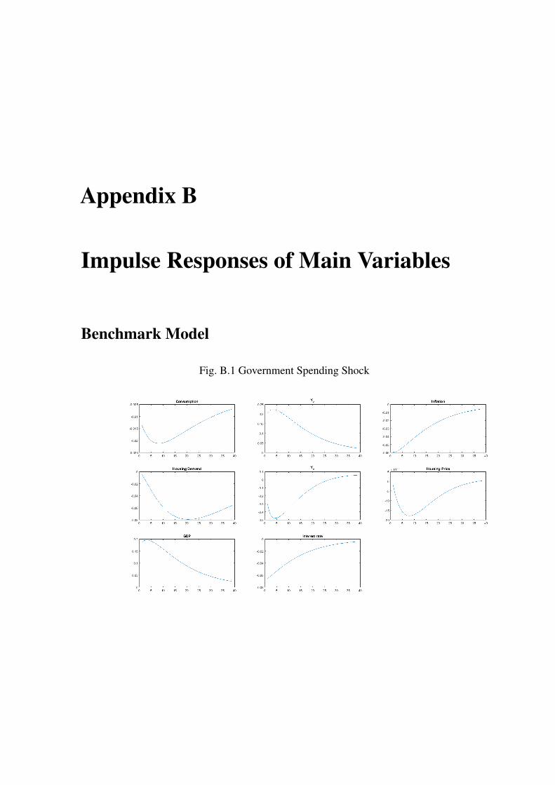
Appendix B
Impulse Responses of Main Variables
Benchmark Model
Fig. B.1 Government Spending Shock

134 Impulse Responses of Main Variables
Fig. B.2 Preference Shock
Fig. B.3 Labour Supply Shock

135
Fig. B.4 Productivity Shock in Housing Sector
Fig. B.5 Labour Demand Shock in General Sector

136 Impulse Responses of Main Variables
Fig. B.6 Capital Demand Shock in General Sector
Fig. B.7 Capital Demand Shock in Housing Sector

137
Model with Collateral Constraint
Fig. B.8 Government Spending Shock
Fig. B.9 Preference Shock

138 Impulse Responses of Main Variables
Fig. B.10 Labour Supply Shock
Fig. B.11 Productivity Shock in Housing Sector

139
Fig. B.12 Labour Demand Shock in General Sector
Fig. B.13 Labour Demand Shock in Housing Sector

140 Impulse Responses of Main Variables
Fig. B.14 Capital Demand Shock in General Sector
Fig. B.15 Capital Demand Shock in Housing Sector
Recommended