Testing the CAPM:
developed vs. emerging
markets
Alexander Tholenaar
Supervisor: Guilherme de Oliveira
University of Amsterdam
Faculty of Economics and Business
Bachelor thesis Economics and Finance
Abstract
The capital asset pricing model (CAPM) is one of the most important models in asset pricing.
Since it has been introduced, the model has often been tested mostly in developed
countries, only a few researchers tried to test the model in emerging countries. In this study
it is questioned whether the CAPM is a better predictor in developed markets than in
emerging markets. The results show that when a local index is used in emerging markets,
the CAPM performs just as good in emerging markets as in developed markets.

1. Introduction
Ever since the capital asset pricing model (CAPM) is introduced by Sharpe (1964) and
Lintner (1965), it has been widely tested by researchers from all over the world. Although
most of the research rejected the model, it is still the most popular model for estimating the
expected return of an asset.
The CAPM explains the relation between return and risk in a linear model. The model
suggests that the expected return can be predicted by the risk free rate and the assets beta.
In the early empirical tests, a static version of the model is tested where the beta does not
vary through time, these tests firmly rejected the model. Two decades later it is argued that
the beta does vary through time and a conditional model with time varying betas is tested.
These tests gave some evidence in favor of the CAPM.
Almost all research that tested the CAPM has been done in developed countries,
especially in the United States. Only some tests are performed in emerging countries. The
results of these studies are contradictory, some of them found evidence in favor of the model
and some did not.
The previous tests of the model gave different outcomes, for both developed and
emerging markets. From these previous tests it is unclear if the model is a better predictor in
developed or in emerging markets. For investors it is relevant to know in which markets the
CAPM works. As a result, the central research question in this paper is:
Does the CAPM predict stock returns better in developed markets than in emerging
markets?
To test this question, this paper uses weekly portfolio returns rather than individual
assets returns. Portfolio betas and expected returns are calculated according to equation
(11) and (12) respectively. Than a regression can be performed of the realized returns on
the expected CAPM returns, when it is found that this regression line is equal to the identity
line than the conclusion can be made that that the CAPM is a good predictor of asset
returns. The expected outcome of this regression is that this regression line is closer to the
identity line for developed markets than in emerging markets.
In contradiction to our expectation we found that the CAPM model works in both
markets, as long as a local market index is used in emerging markets.
The paper begins by explaining the CAPM, followed by some summarizing literature.
Section 3 presents the data that is used and in section 4 the methodology is explained. In
section 5 the results from the regressions are interpreted. Finally, a conclusion will be drawn
in section 6.
2. Literature review
2.1 Theoretical background
In this paragraph the basic fundamentals and the origins of the CAPM are discussed
followed by the main equation of the model.
The foundations of the CAPM developed by Sharpe (1964) and Lintner (1965) are to
be found in the paper introduced by Markowitz (1952). In his paper he begins by rejecting
the assumption that investors should only maximize the discounted expected return. He
argues that investors should care, about the variance of returns besides expected return. He
states that investors should build portfolios by 1) maximizing expected returns given
variances and 2) minimize the variance of return given expected return. This is known as
“mean-variance-efficient” portfolios.
Tobin (1958) expanded the model of Markowitz by introducing lending at a risk-free
rate. Tobin states that the portfolio choice is separated into two stages. The first stage is to
find the efficient portfolio of risky assets; in the second stage, the investor has to find the
optimum fractions of risk-free lending and the risky portfolio that meets his/her risk
preference.
By adding two key assumptions to the model, first formulated by Markowitz and later
extended by Tobin, Sharpe (1964) and Lintner (1965) introduced their famous capital asset
pricing model (hereafter CAPM). The first assumption is that investors have a joint
probability distribution, so each investor has the same and true distribution function. The
second assumption is that every investor can borrow and lend at the same risk-free rate,
Tobin (1958) only assumed lending.
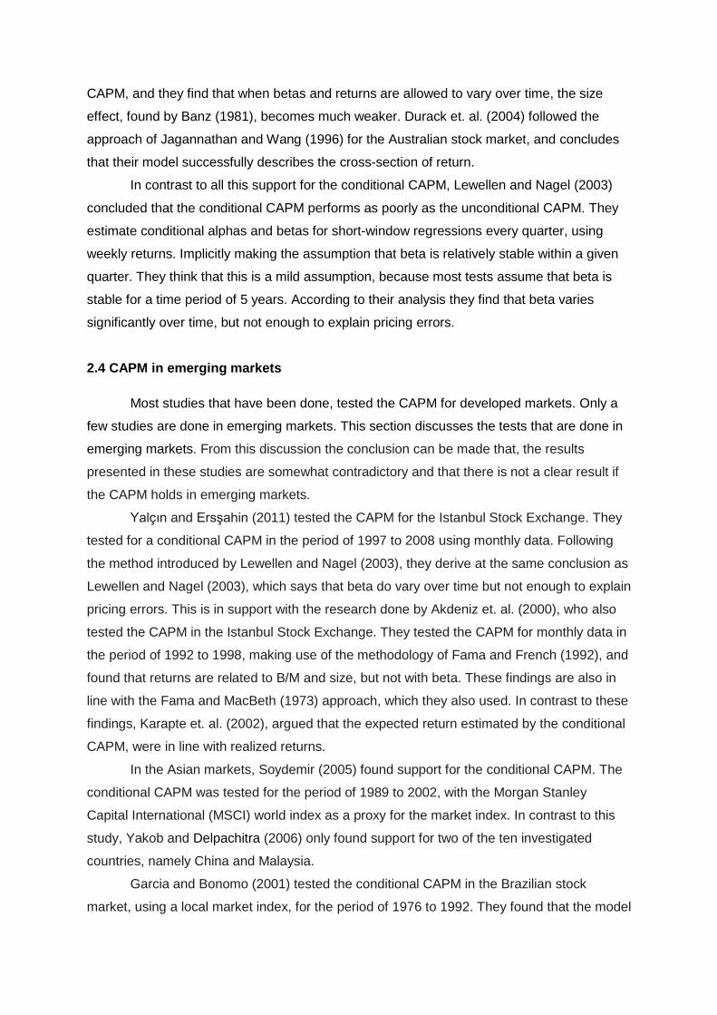
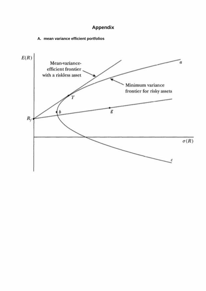
Figure 1 in appendix A shows this story graphically. The curve 'abc’ is the curve that,
for different levels of expected return, minimizes the variance of risky portfolios and is called
the minimum variance frontier. By adding risk-free borrowing and lending, the set of efficient
portfolio becomes a straight line. To derive the mean-variance efficient portfolio with a risk-
less asset, one needs to draw a straight line from Rf up to the left as far as possible until it is
tangent with the minimum variance frontier. The tangent point is called the tangency
portfolio, indicated by T. Because all investors have the same probability distribution and can
borrow and lend at the same risk-free rate, all investors hold the same tangency portfolio T.
Since all investors are holding the same portfolio T, it must be the case that this portfolio is
equal to the value-weighted market portfolio (Fama and French, 2004). Only the level of
preferred risk, observed by the fraction x invested in the risk-free asset, makes the difference
in investors’ portfolios. Since the assumptions made by Sharpe (1964) and Lintner (1965)

imply that the market portfolio lies on the minimum-variance frontier, the relationship that
holds for minimum-variance frontier must also hold for the market portfolio.
The minimum-variance condition can be algebraically formulated in the following
equation,
(𝑅𝑖) = 𝐸(𝑅𝑍𝑀) + 𝛽𝑖𝑀[𝐸(𝑅𝑀) − 𝐸(𝑅𝑍𝑀)] (1)
Where E(Ri) is the expected return on asset i, E(RZM) is the expected return of an asset that
is uncorrelated with the market return. The last term is called the risk premium and the beta
term is the covariance of asset i and the market portfolio M relative to the variance of the
market portfolio,
𝛽𝑖𝑀 =𝐶𝑜𝑣(𝑅𝑖,𝑅𝑀)
𝑉𝑎𝑟(𝑅𝑀) (2)
This beta term can be interpreted as the sensitivity of the assets return to variation in the
market portfolio, which means it can be seen as a risk measure.
To derive at the well-known Sharpe-Lintner CAPM equation, one must bring in the
assumption of risk-free borrowing and lending. When a risky asset is uncorrelated with the
market, this risky asset is riskless in the market portfolio because it adds nothing to the
variance of the market return. By introducing risk-free borrowing and lending, the expected
return of this asset that is uncorrelated with the market return must equal the risk-free rate,
Rf. and the following equation can be derived,
𝐸(𝑅𝑖) = 𝑅𝑓 + 𝛽𝑖[𝐸(𝑅𝑀) − 𝑅𝑓] (3)
2.2 Conditional CAPM
In this paragraph an extension of the basic (static) CAPM will be introduced which
allow beta to vary over time.
In the early empirical tests of the CAPM, researchers assumed that the beta remains
constant over time and tested for a static model. However in the eighties researchers tried to
determine the importance of changing risk premia and returns variability over time. Bodurtha
and Mark (1991) and Ng (1991) incorporated these variabilities that other researchers have
found into a conditional CAPM where the beta does vary over time. This conditional model
states that risk and return on time t are conditioned on the information set available at t-1.
Both papers followed a different approach in testing the model, but both found evidence that
support the conditional version of the CAPM.
2.2 CAPM in developed markets
In this section the main literature that tested the CAPM in developed markets are
summarized. The conclusion that can be drawn from these studies is that, it is not clear
whether the CAPM holds in developed markets. Although the conditional CAPM performs
perhaps as poorly as the unconditional CAPM, betas do vary over time.
Ever since the CAPM is introduced it has been widely tested by researchers
worldwide. One of the earliest tests were done by Black, Jensen and Scholes (1972). They
stated that the cross-section tests done by Douglas (1969) and later by Miller and Scholes
(1972) can be misleading and therefore do not provide direct tests of the validity of the
model. Instead Black, Jensen and Scholes (1972) performed a time-series test, which is free
of the problems that come with a cross-section test. They perform regressions with monthly
data, for every stock listed on the New York stock exchange in the period from 1926 to 1966,
on portfolios based on a beta ranking system. First they estimated the betas for the period
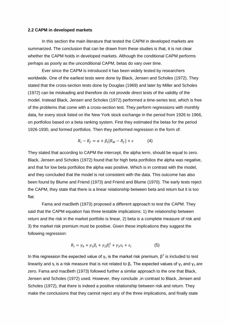
1926-1930, and formed portfolios. Then they performed regression in the form of:
𝑅𝑖 − 𝑅𝑓 = 𝛼 + 𝛽𝑖[𝑅𝑀 − 𝑅𝑓] + 휀 (4)
They stated that according to CAPM the intercept, the alpha term, should be equal to zero.
Black, Jensen and Scholes (1972) found that for high beta portfolios the alpha was negative,
and that for low beta portfolios the alpha was positive. Which is in contrast with the model,
and they concluded that the model is not consistent with the data. This outcome has also
been found by Blume and Friend (1973) and Friend and Blume (1970). The early tests reject
the CAPM, they state that there is a linear relationship between beta and return but it is too
flat.
Fama and macBeth (1973) proposed a different approach to test the CAPM. They
said that the CAPM equation has three testable implications: 1) the relationship between
return and the risk in the market portfolio is linear, 2) beta is a complete measure of risk and
3) the market risk premium must be positive. Given these implications they suggest the
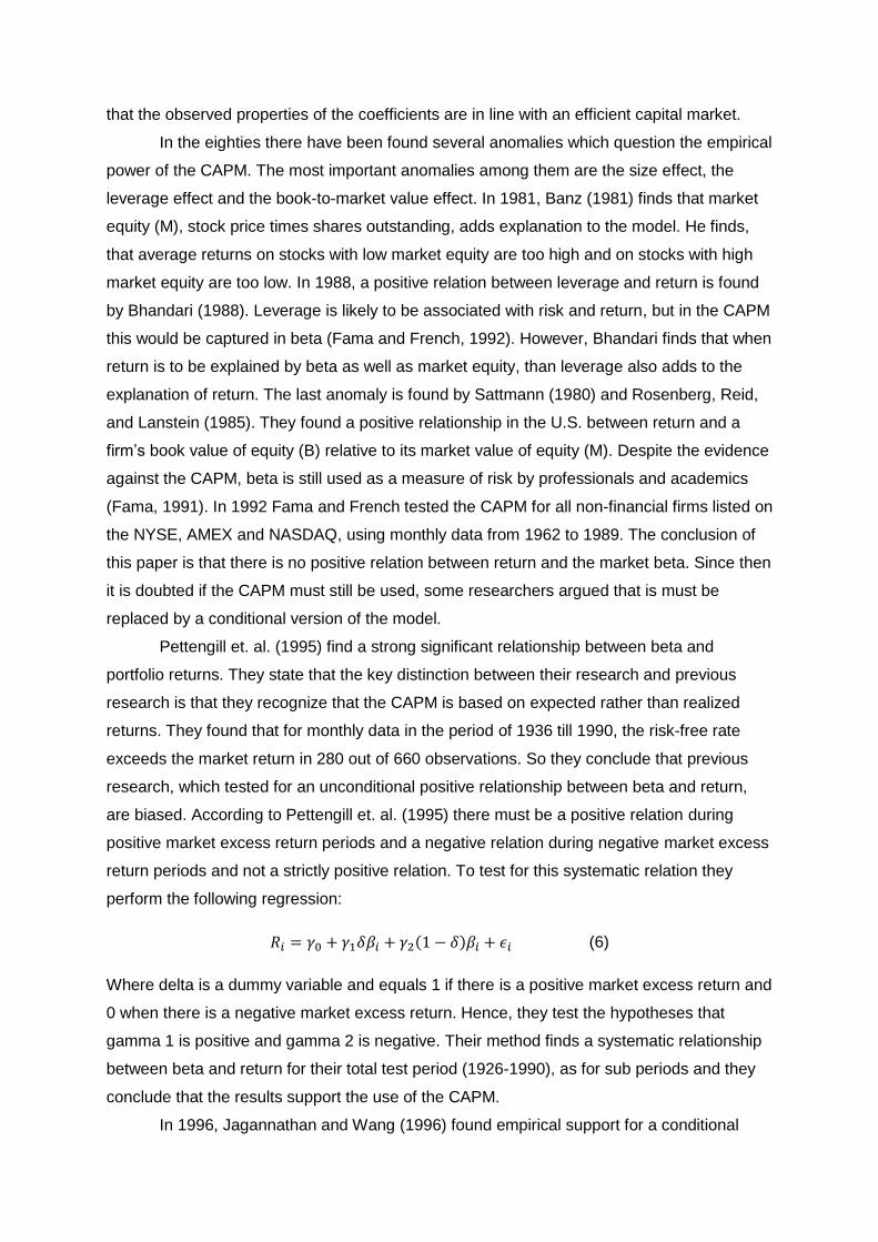
following regression:
𝑅𝑖 = 𝛾0 + 𝛾1𝛽𝑖 + 𝛾2𝛽𝑖2 + 𝛾3𝑠𝑖 + 휀𝑖 (5)
In this regression the expected value of γ1 is the market risk premium, β2 is included to test
linearity and si is a risk measure that is not related to βi. The expected values of γ2 and γ3 are
zero. Fama and macBeth (1973) followed further a similar approach to the one that Black,
Jensen and Scholes (1972) used. However, they conclude ,in contrast to Black, Jensen and
Scholes (1972), that there is indeed a positive relationship between risk and return. They
make the conclusions that they cannot reject any of the three implications, and finally state
that the observed properties of the coefficients are in line with an efficient capital market.
In the eighties there have been found several anomalies which question the empirical
power of the CAPM. The most important anomalies among them are the size effect, the
leverage effect and the book-to-market value effect. In 1981, Banz (1981) finds that market
equity (M), stock price times shares outstanding, adds explanation to the model. He finds,
that average returns on stocks with low market equity are too high and on stocks with high
market equity are too low. In 1988, a positive relation between leverage and return is found
by Bhandari (1988). Leverage is likely to be associated with risk and return, but in the CAPM
this would be captured in beta (Fama and French, 1992). However, Bhandari finds that when
return is to be explained by beta as well as market equity, than leverage also adds to the
explanation of return. The last anomaly is found by Sattmann (1980) and Rosenberg, Reid,
and Lanstein (1985). They found a positive relationship in the U.S. between return and a
firm’s book value of equity (B) relative to its market value of equity (M). Despite the evidence
against the CAPM, beta is still used as a measure of risk by professionals and academics
(Fama, 1991). In 1992 Fama and French tested the CAPM for all non-financial firms listed on
the NYSE, AMEX and NASDAQ, using monthly data from 1962 to 1989. The conclusion of
this paper is that there is no positive relation between return and the market beta. Since then
it is doubted if the CAPM must still be used, some researchers argued that is must be
replaced by a conditional version of the model.
Pettengill et. al. (1995) find a strong significant relationship between beta and
portfolio returns. They state that the key distinction between their research and previous
research is that they recognize that the CAPM is based on expected rather than realized
returns. They found that for monthly data in the period of 1936 till 1990, the risk-free rate
exceeds the market return in 280 out of 660 observations. So they conclude that previous
research, which tested for an unconditional positive relationship between beta and return,
are biased. According to Pettengill et. al. (1995) there must be a positive relation during
positive market excess return periods and a negative relation during negative market excess
return periods and not a strictly positive relation. To test for this systematic relation they
perform the following regression:
𝑅𝑖 = 𝛾0 + 𝛾1𝛿𝛽𝑖 + 𝛾2(1 − 𝛿)𝛽𝑖 + 𝜖𝑖 (6)
Where delta is a dummy variable and equals 1 if there is a positive market excess return and
0 when there is a negative market excess return. Hence, they test the hypotheses that
gamma 1 is positive and gamma 2 is negative. Their method finds a systematic relationship
between beta and return for their total test period (1926-1990), as for sub periods and they
conclude that the results support the use of the CAPM.
In 1996, Jagannathan and Wang (1996) found empirical support for a conditional
CAPM, and they find that when betas and returns are allowed to vary over time, the size
effect, found by Banz (1981), becomes much weaker. Durack et. al. (2004) followed the
approach of Jagannathan and Wang (1996) for the Australian stock market, and concludes
that their model successfully describes the cross-section of return.
In contrast to all this support for the conditional CAPM, Lewellen and Nagel (2003)
concluded that the conditional CAPM performs as poorly as the unconditional CAPM. They
estimate conditional alphas and betas for short-window regressions every quarter, using
weekly returns. Implicitly making the assumption that beta is relatively stable within a given
quarter. They think that this is a mild assumption, because most tests assume that beta is
stable for a time period of 5 years. According to their analysis they find that beta varies
significantly over time, but not enough to explain pricing errors.
2.4 CAPM in emerging markets
Most studies that have been done, tested the CAPM for developed markets. Only a
few studies are done in emerging markets. This section discusses the tests that are done in
emerging markets. From this discussion the conclusion can be made that, the results
presented in these studies are somewhat contradictory and that there is not a clear result if
the CAPM holds in emerging markets.
Yalçın and Ersşahin (2011) tested the CAPM for the Istanbul Stock Exchange. They
tested for a conditional CAPM in the period of 1997 to 2008 using monthly data. Following
the method introduced by Lewellen and Nagel (2003), they derive at the same conclusion as
Lewellen and Nagel (2003), which says that beta do vary over time but not enough to explain
pricing errors. This is in support with the research done by Akdeniz et. al. (2000), who also
tested the CAPM in the Istanbul Stock Exchange. They tested the CAPM for monthly data in
the period of 1992 to 1998, making use of the methodology of Fama and French (1992), and
found that returns are related to B/M and size, but not with beta. These findings are also in
line with the Fama and MacBeth (1973) approach, which they also used. In contrast to these
findings, Karapte et. al. (2002), argued that the expected return estimated by the conditional
CAPM, were in line with realized returns.
In the Asian markets, Soydemir (2005) found support for the conditional CAPM. The
conditional CAPM was tested for the period of 1989 to 2002, with the Morgan Stanley
Capital International (MSCI) world index as a proxy for the market index. In contrast to this
study, Yakob and Delpachitra (2006) only found support for two of the ten investigated
countries, namely China and Malaysia.
Garcia and Bonomo (2001) tested the conditional CAPM in the Brazilian stock
market, using a local market index, for the period of 1976 to 1992. They found that the model
is supported by their dataset. In contrast to this result found by Garcia and Bonomo (2001),
Yoshino (2009) concluded that the CAPM is not supported with the data. He performed
regressions using data from 1998 to 2006, making use of the same local market index as
Garcia and Bonomo (2001). Yoshino made the conclusion that the CAPM is not supported
for two reasons. First, the intercept of the security market line is not zero, and second, he
finds other variables, such as size and B/M, that add explanatory value to the model.
2.5 Developed versus emerging markets
The previous studies that tested the validity of the CAPM did not investigated the
validity in both markets, some studies tested the CAPM only in developed markets and some
tested the CAPM only in emerging markets. The studies that tested the CAPM in developed
markets gave contradictory conclusions, some did gave evidence in favor of the CAPM and
others did not. For the studies that investigated the CAPM in emerging markets the same
conclusions are given as in the developed markets. From the previous literature it is not
clear if the CAPM works in both markets, consequently we cannot draw a straight conclusion
whether the CAPM works better in a developed market or in an emerging market.
3. Data
3.1 Sample overview
This paper examines whether the CAPM holds better in developed countries than in
emerging countries from a time period of July 1994 till June 2016. Weekly returns from 38
stocks in Australia, 12 in Brazil, 21 in Hong Kong and 15 in The Netherlands have been
used, this difference in stock quantities is due to availability of stock prices in the period that
this paper uses. If a later time period would be chosen to increase the number of stocks,
then this increase in the number of stocks would be relatively small comparing to the
decrease in the time period . The stock opening prices are collected from the UvA
DataStream database. In total there are 1143 data points collected for each stock. Weekly
returns are being used because not all stocks around the world are traded every day. So
there would be a lot of missing data points in data of daily returns. Weekly returns diminishes
this.
3.2 Market proxy
To estimate the expected return proposed by the CAPM, one needs to have the
expected return of the market portfolio. This market portfolio is difficult to observe because
not all assets are marketable, such as human capital and private business (Mirza and
Shabbir, 2005). The outcome of this is that if one wants to test the CAPM he/she is
constrained to use a proxy for the market portfolio (Fama and French, 2004, p. 25). For
developed countries this paper assumes that these stocks are intergraded in the world
market, so for these stocks only the MSCI world index, maintained by Morgan Stanley
Capital International (MSCI) and containing 1643 stocks from 23 countries, is used as a
proxy for the market portfolio. For emerging markets the assumption of world market
integration is doubted. So for the two emerging markets there will be two test, namely one
that assumes world market integration and uses the MSCI world index as a proxy for the
market portfolio, and the other which do not assumes world integration and uses the local
market index, being the MSCI Brazil index for Brazil and the Hang Seng index for Hong
Kong.
3.3 Risk-free rate
The risk-free rate used in this paper is the 3-month rate of US Treasury Bills. The
rates are adjusted from annually to weekly as followed:
𝑅𝑓 = (1 + 3 𝑚𝑜𝑛𝑡ℎ 𝑟𝑎𝑡𝑒)1/52 − 1 (7)
4. Methodology
This paper does not investigate the linear risk-return trade-off, it tests if the model is
a better predictor in developed markets than in emerging markets. So the methods used in
the previous papers do not apply in this paper, instead this paper uses a different approach.
4 steps are followed to test in which country/countries applies the CAPM the best.
1) Previous tests of the CAPM such as those performed by Blume (1970) and Black,
Jensen and Scholes (1972) suggested that the precision of the estimated is improved
by using portfolios instead of individual stocks.
Estimates for diversified portfolios are more precise than for individual assets
(Fama, French, 2004, p.31), this is due to the fact that beta estimates give a
measurement error. Black, Jensen and Scholes (1972) claimed that if the estimation
errors are uncorrelated among stocks, the effect of this measurement error in
portfolio betas could be reduced.
In the first step, unconditional betas are estimated using the full time series of
return, and are ranked from small to large. Then portfolios are being formed
according to the ranking in beta, within each country . Starting with the portfolio that
contains the lowest beta stocks, up to the last portfolio that contains the highest beta
stocks. This sorting procedure is standard in empirical tests (Fama and French,
2004).
2) The second step is to calculate the return of each portfolio according to the following
formula:
𝑅𝑃𝑖 =1
𝑁∑ 𝑅𝑖
𝑁𝑖=1 (10)
3) The third step is to calculate the conditional portfolio betas. The portfolio beta’s are
being calculated every day from July 1994 until June 2016 using the weekly returns
of the previous 52 weeks, given:
𝛽𝑃𝑖 =𝐶𝑜𝑣(𝑅𝑝𝑖,𝑅𝑀)
𝑉𝑎𝑟(𝑅𝑀) (11)
4) Given these portfolio beta’s one can calculate the expected return given by the
CAPM equation:
𝐸(𝑅𝑝𝑖) = 𝑅𝑓 + 𝛽𝑃[𝐸(𝑅𝑀) − 𝑅𝑓] (12)
From this a regression of the given historical realized portfolio return on the expected
return imposed by the CAPM can be performed:
𝑅𝑃𝑖 = 𝛼�̂� + 𝛾�̂�𝐸(𝑅𝑃𝑖) + 휀𝑖 (13)
Implicating that when 𝛼𝑖 = 0 𝑎𝑛𝑑 𝛾�̂� = 1 the CAPM gives a good estimate of stock
returns.
Besides these 4 steps there will also be a two-sided Z-test1 of comparing averages
performed. The idea comes from a paper written by Karatepe et. al. in 2002. In this paper
they tested the conditional CAPM for the Istanbul stock exchange. The assumption is made
that the data fit in the normal distribution, because n>30, which is in line with the Central limit
theorem.
According to these methods several hypotheses will be formed, given below.
Hypothesis 1:
H0: αi=0
H1: αi≠0
Hypothesis 2:
H0: γi=1
H1: γi≠1
Hypothesis 3:
H0: Ri-Ri*2=0
H1: Ri-Ri*≠0
1 𝑧 =
𝑥1̅̅̅̅ −𝑥2̅̅̅̅ −0
√𝜎1
2
𝑛1+
𝜎22
𝑛2
2 Ri
* equals the expected return on asset i according to CAPM
5. Results
In this section the main results will be discussed. It is found that for most portfolios
the CAPM holds in developed markets. For the emerging markets the CAPM does not hold
when world market integration is assumed, but when a local market index is used as a proxy
for the market portfolio, the model works just as well as in developed markets.
Using equation (2), each stock unconditional beta is calculated and the results are
presented in appendix B. According to this table portfolios are being formed, as explained in
section 4. After this forming of portfolios, daily changing betas of each portfolio are
calculated using equation (11). With these betas the expected return of each portfolio can be
calculated according to CAPM for each day by using equation (12), some descriptive
statistics are presented in appendix B. According to the CAPM, high beta portfolios must
also have a higher expected return. As we can see from the graph in appendix F this
relationship can clearly be seen. Now that we know the expected returns according to CAPM
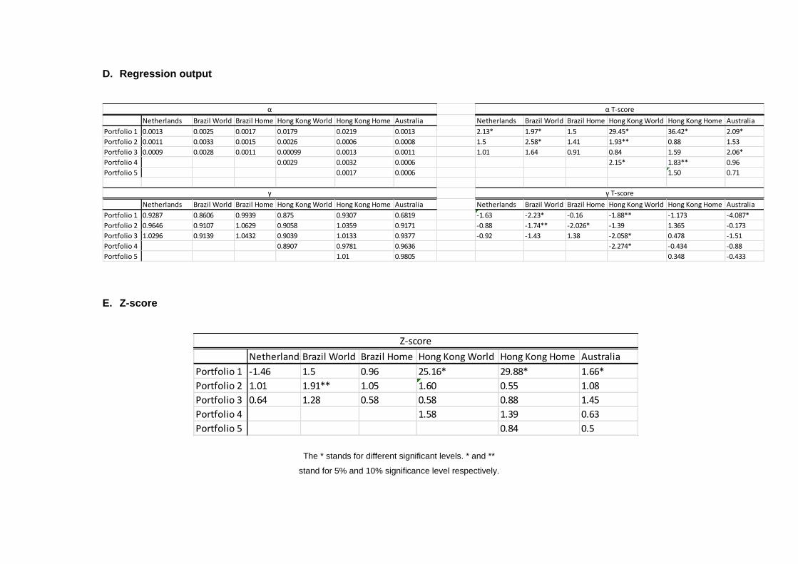
for each day, regression (13) can be performed. The results from the regression output are
presented in appendix D. The expected CAPM returns reflects the realized if 𝛼𝑖 = 0 𝑎𝑛𝑑 𝛾�̂� =
1.
Using the t-statistic3, the following portfolios in the developed markets reject the null
of hypothesis 1:
1) for a 5% critical value:
Netherlands: 1
Australia: 1 and 3
The following portfolios in the developed markets reject the null of hypothesis 2:
1) for a 5% critical value
Australia: 1
The following portfolios in the emerging markets reject the null of hypothesis 1:
1) for a 5% critical value
Brazil World: 1 and 2
Hong Kong World: 1 and 4
Hong Kong Home: 1
3 𝑡(𝛾�̂�) =
𝛾�̂�−1
𝑠(𝛾�̂�) , 𝑡(𝛼�̂�) =
𝛼�̂�−0
𝑠(𝛼�̂�)
2) for a 10% critical value
Hong Kong World: 2
Hong Kong Home: 4
The following portfolios in the emerging markets reject the null of hypothesis 2:
1) for a 5% critical value
Brazil World: 1
Brazil Home: 2
Hong Kong World: 3 and 4
2) for a 10% critical value
Brazil World: 2
Hong Kong World: 1
From this the conclusion can be drawn that for portfolios 1 and 2 in Brazil the CAPM with the
world market portfolio do not give a good representation of the realized return. The same
applies for all portfolios in Hong Kong given the world market and also for portfolio 1 in
Australia.
According to the results of the Z-tests, presented in appendix E, the null of
hypothesis 3 is rejected at the 5% level for both portfolios 1 in Hong Kong and Australia and
at the 10% level for portfolio 2 in Brazil estimated with the world index. These results imply
that for almost every portfolio the CAPM gives a good representation of the realized returns.
These findings are in line with some of the previous literature. The results are in line
with the research done by Garcia and Bonomo (2001), who also found that when using a
local market index the CAPM gives a good approximation of the realized returns in Brazil.
Our results are however in contrast with the results presented by Soydemir (2005), who
supported the model in Asia by using the MSCI world index. Our study used the same world
market index, but come to the conclusion that the model is not supported in Hong Kong.
6. Conclusion
This paper investigated if the CAPM predicts stock returns better in developed
markets or in emerging markets. It is found that the CAPM is valid in both developed and
emerging markets, as long as the local index is used as a proxy for the market portfolio in
emerging markets.
The results show that the expected returns according to CAPM are a good
approximation of realized return in developed markets. The null of hypothesis 1 is only
rejected for portfolio 1 in the Netherlands and for portfolio 1 and 3 in Australia. The null of
hypothesis 2 and 3 is only rejected for portfolio 1 in Australia.
In the emerging markets the CAPM returns give a good approximation of the realized
returns as long as the local market index is used for a proxy of the market portfolio. The null
of hypothesis 1 and 2 is for almost every portfolio, regressed with the world index, rejected.
Almost none portfolio, regressed on the local index, rejected the null of hypothesis 1 and 2.
This paper tested whether the CAPM predicts stock returns better in developed
markets or in emerging markets for the period of 1994 till 2016. Further research can
perform tests for sub periods to see if the CAPM begins to work better as a market becomes
more mature.
References
Akdeniz, L., Altay-Salih, A., & Aydogan, K. (2000). A cross-section of expected stock
returns on the Istanbul stock exchange. Russian & East European Finance and Trade, 36(5),
6-26.
Black, F. (1972). Capital market equilibrium with restricted borrowing. The Journal of
Business, 45(3), 444-455.
Blume, M. E. (1970). Portfolio theory: a step toward its practical application.The
Journal of Business, 43(2), 152-173.
Bodurtha, J. N., & Mark, N. C. (1991). Testing the CAPM with Time‐Varying risks and
returns. The Journal of Finance, 46(4), 1485-1505.
Douglas, G. W. (1968). Risk in the Equity Markets: An Empirical Appraisal of Market
Effeciency. University Microfilms, Incorporated.
Durack, N., Durand, R. B., & Maller, R. A. (2004). A best choice among asset pricing
models? The conditional capital asset pricing model in Australia. Accounting &
Finance, 44(2), 139-162.
Fama, E. F. (1991). Efficient capital markets: II. The journal of finance,46(5), 1575-
1617.
Fama, E. F., & French, K. R. (2004). The capital asset pricing model: Theory and
evidence. Journal of Economic Perspectives, 18, 25-46.
Fama, E. F., & MacBeth, J. D. (1973). Risk, return, and equilibrium: Empirical
tests. The Journal of Political Economy, 607-636.
Garcia, R., & Bonomo, M. (2001). Tests of conditional asset pricing models in the
Brazilian stock market. Journal of International Money and Finance, 20(1), 71-90.
Jensen, M. C., Black, F., & Scholes, M. S. (1972). The capital asset pricing model:
Some empirical tests.
Karatepe, Y., Karaaslan, E., & Gokgoz, F. (2002). Conditional CAPM and an
Application on the ISE. Istanbul Stock Exchange Review, 6(21), 21-36.
Lewellen, J., & Nagel, S. (2006). The conditional CAPM does not explain asset-
pricing anomalies. Journal of financial economics, 82(2), 289-314.
Lintner, J. (1965). The valuation of risk assets and the selection of risky investments
in stock portfolios and capital budgets. The review of economics and statistics, 13-37.
Markowitz, H. (1952). Portfolio selection. The journal of finance, 7(1), 77-91.
Miller, M. H., & Scholes, M. (1972). Rates of return in relation to risk: A reexamination
of some recent findings. Studies in the theory of capital markets, 23.
Mirza, N., & Shabbir, G. (2005). The death of CAPM: A critical review. Lahore J.
Econ, 10(2), 35-54.
Ng, L. (1991). Tests of the CAPM with time‐varying covariances: A multivariate
GARCH approach. The Journal of Finance, 46(4), 1507-1521.
Olakojo, S. A., & Ajide, K. B. (2010). Testing the Capital Asset Pricing Model
(CAPM): The Case of the Nigerian Securities Market. International Business
Management, 4(4), 239-242.
Pettengill, G. N., Sundaram, S., & Mathur, I. (1995). The conditional relation between
beta and returns. Journal of Financial and quantitative Analysis,30(01), 101-116.
Sharpe, W. F. (1964). Capital asset prices: A theory of market equilibrium under
conditions of risk. The journal of finance, 19(3), 425-442.
Soydemir, G. A. (2005). Differences in the price of risk and the resulting response to
shocks: an analysis of Asian markets. Journal of International Financial Markets, Institutions
and Money, 15(4), 285-313.
Tobin, J. (1958). Liquidity preference as behavior towards risk. The review of
economic studies, 25(2), 65-86.
Yalçın, A., & Ersşahin, N. (2011). Does the conditional CAPM work? Evidence from
the Istanbul Stock Exchange. Emerging Markets Finance and Trade, 47(4), 28-48.
Yakob, N. A., & Delpachitra, S. (2007). On risk-return relationship: an application of
GARCH (p, q)-M model to Asia _ Pacific region. International Journal of Science and
Research, 2(1), 33-39.
Yoshino, J. A. (2009). Is CAPM Dead or Alive in the Brazilian Equity Market?.Review
of Applied Economics, 5(1), 127.
Appendix
A. mean variance efficient portfolios
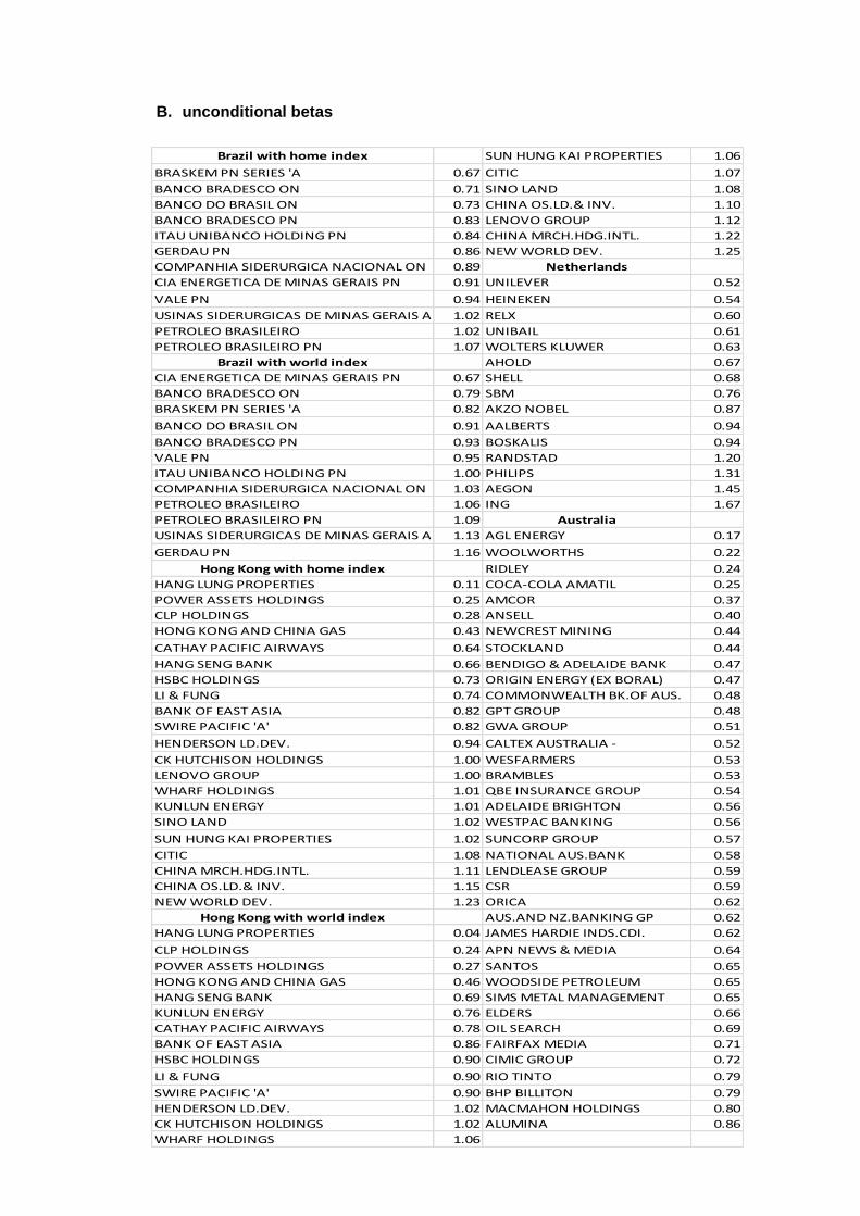
B. unconditional betas
Brazil with home index SUN HUNG KAI PROPERTIES 1.06
BRASKEM PN SERIES 'A 0.67 CITIC 1.07
BANCO BRADESCO ON 0.71 SINO LAND 1.08
BANCO DO BRASIL ON 0.73 CHINA OS.LD.& INV. 1.10
BANCO BRADESCO PN 0.83 LENOVO GROUP 1.12
ITAU UNIBANCO HOLDING PN 0.84 CHINA MRCH.HDG.INTL. 1.22
GERDAU PN 0.86 NEW WORLD DEV. 1.25
COMPANHIA SIDERURGICA NACIONAL ON 0.89 Netherlands
CIA ENERGETICA DE MINAS GERAIS PN 0.91 UNILEVER 0.52
VALE PN 0.94 HEINEKEN 0.54
USINAS SIDERURGICAS DE MINAS GERAIS A PN1.02 RELX 0.60
PETROLEO BRASILEIRO 1.02 UNIBAIL 0.61
PETROLEO BRASILEIRO PN 1.07 WOLTERS KLUWER 0.63
Brazil with world index AHOLD 0.67
CIA ENERGETICA DE MINAS GERAIS PN 0.67 SHELL 0.68
BANCO BRADESCO ON 0.79 SBM 0.76
BRASKEM PN SERIES 'A 0.82 AKZO NOBEL 0.87
BANCO DO BRASIL ON 0.91 AALBERTS 0.94
BANCO BRADESCO PN 0.93 BOSKALIS 0.94
VALE PN 0.95 RANDSTAD 1.20
ITAU UNIBANCO HOLDING PN 1.00 PHILIPS 1.31
COMPANHIA SIDERURGICA NACIONAL ON 1.03 AEGON 1.45
PETROLEO BRASILEIRO 1.06 ING 1.67
PETROLEO BRASILEIRO PN 1.09 Australia
USINAS SIDERURGICAS DE MINAS GERAIS A PN1.13 AGL ENERGY 0.17
GERDAU PN 1.16 WOOLWORTHS 0.22
Hong Kong with home index RIDLEY 0.24
HANG LUNG PROPERTIES 0.11 COCA-COLA AMATIL 0.25
POWER ASSETS HOLDINGS 0.25 AMCOR 0.37
CLP HOLDINGS 0.28 ANSELL 0.40
HONG KONG AND CHINA GAS 0.43 NEWCREST MINING 0.44
CATHAY PACIFIC AIRWAYS 0.64 STOCKLAND 0.44
HANG SENG BANK 0.66 BENDIGO & ADELAIDE BANK 0.47
HSBC HOLDINGS 0.73 ORIGIN ENERGY (EX BORAL) 0.47
LI & FUNG 0.74 COMMONWEALTH BK.OF AUS. 0.48
BANK OF EAST ASIA 0.82 GPT GROUP 0.48
SWIRE PACIFIC 'A' 0.82 GWA GROUP 0.51
HENDERSON LD.DEV. 0.94 CALTEX AUSTRALIA - 0.52
CK HUTCHISON HOLDINGS 1.00 WESFARMERS 0.53
LENOVO GROUP 1.00 BRAMBLES 0.53
WHARF HOLDINGS 1.01 QBE INSURANCE GROUP 0.54
KUNLUN ENERGY 1.01 ADELAIDE BRIGHTON 0.56
SINO LAND 1.02 WESTPAC BANKING 0.56
SUN HUNG KAI PROPERTIES 1.02 SUNCORP GROUP 0.57
CITIC 1.08 NATIONAL AUS.BANK 0.58
CHINA MRCH.HDG.INTL. 1.11 LENDLEASE GROUP 0.59
CHINA OS.LD.& INV. 1.15 CSR 0.59
NEW WORLD DEV. 1.23 ORICA 0.62
Hong Kong with world index AUS.AND NZ.BANKING GP 0.62
HANG LUNG PROPERTIES 0.04 JAMES HARDIE INDS.CDI. 0.62
CLP HOLDINGS 0.24 APN NEWS & MEDIA 0.64
POWER ASSETS HOLDINGS 0.27 SANTOS 0.65
HONG KONG AND CHINA GAS 0.46 WOODSIDE PETROLEUM 0.65
HANG SENG BANK 0.69 SIMS METAL MANAGEMENT 0.65
KUNLUN ENERGY 0.76 ELDERS 0.66
CATHAY PACIFIC AIRWAYS 0.78 OIL SEARCH 0.69
BANK OF EAST ASIA 0.86 FAIRFAX MEDIA 0.71
HSBC HOLDINGS 0.90 CIMIC GROUP 0.72
LI & FUNG 0.90 RIO TINTO 0.79
SWIRE PACIFIC 'A' 0.90 BHP BILLITON 0.79
HENDERSON LD.DEV. 1.02 MACMAHON HOLDINGS 0.80
CK HUTCHISON HOLDINGS 1.02 ALUMINA 0.86
WHARF HOLDINGS 1.06
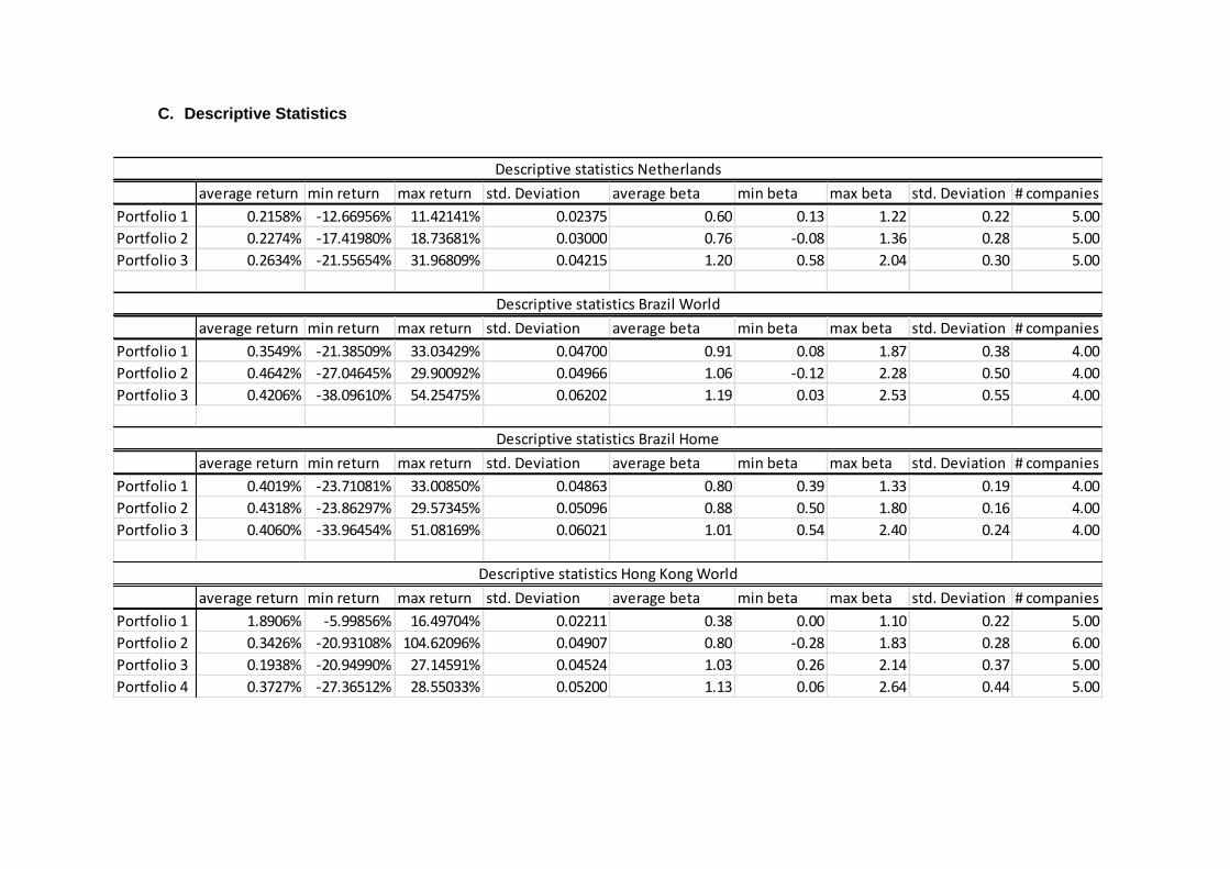
C. Descriptive Statistics
average return min return max return std. Deviation average beta min beta max beta std. Deviation # companies
Portfolio 1 0.2158% -12.66956% 11.42141% 0.02375 0.60 0.13 1.22 0.22 5.00
Portfolio 2 0.2274% -17.41980% 18.73681% 0.03000 0.76 -0.08 1.36 0.28 5.00
Portfolio 3 0.2634% -21.55654% 31.96809% 0.04215 1.20 0.58 2.04 0.30 5.00
average return min return max return std. Deviation average beta min beta max beta std. Deviation # companies
Portfolio 1 0.3549% -21.38509% 33.03429% 0.04700 0.91 0.08 1.87 0.38 4.00
Portfolio 2 0.4642% -27.04645% 29.90092% 0.04966 1.06 -0.12 2.28 0.50 4.00
Portfolio 3 0.4206% -38.09610% 54.25475% 0.06202 1.19 0.03 2.53 0.55 4.00
average return min return max return std. Deviation average beta min beta max beta std. Deviation # companies
Portfolio 1 0.4019% -23.71081% 33.00850% 0.04863 0.80 0.39 1.33 0.19 4.00
Portfolio 2 0.4318% -23.86297% 29.57345% 0.05096 0.88 0.50 1.80 0.16 4.00
Portfolio 3 0.4060% -33.96454% 51.08169% 0.06021 1.01 0.54 2.40 0.24 4.00
average return min return max return std. Deviation average beta min beta max beta std. Deviation # companies
Portfolio 1 1.8906% -5.99856% 16.49704% 0.02211 0.38 0.00 1.10 0.22 5.00
Portfolio 2 0.3426% -20.93108% 104.62096% 0.04907 0.80 -0.28 1.83 0.28 6.00
Portfolio 3 0.1938% -20.94990% 27.14591% 0.04524 1.03 0.26 2.14 0.37 5.00
Portfolio 4 0.3727% -27.36512% 28.55033% 0.05200 1.13 0.06 2.64 0.44 5.00
Descriptive statistics Hong Kong World
Descriptive statistics Netherlands
Descriptive statistics Brazil World
Descriptive statistics Brazil Home
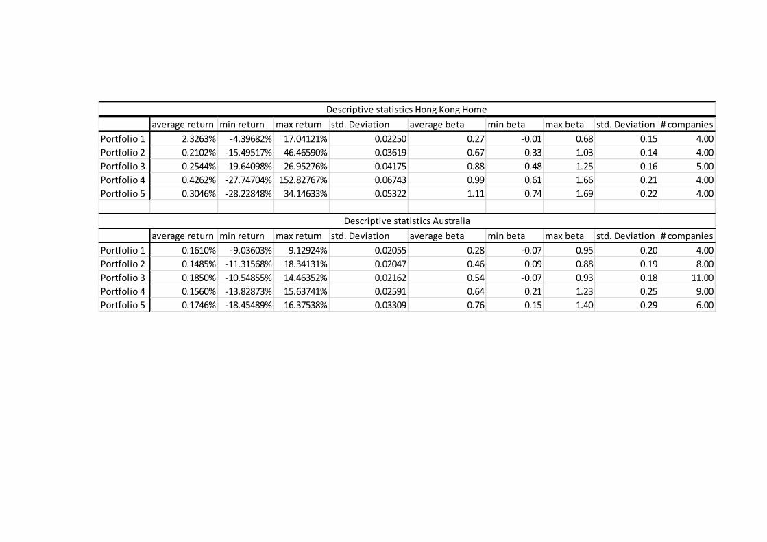
average return min return max return std. Deviation average beta min beta max beta std. Deviation # companies
Portfolio 1 2.3263% -4.39682% 17.04121% 0.02250 0.27 -0.01 0.68 0.15 4.00
Portfolio 2 0.2102% -15.49517% 46.46590% 0.03619 0.67 0.33 1.03 0.14 4.00
Portfolio 3 0.2544% -19.64098% 26.95276% 0.04175 0.88 0.48 1.25 0.16 5.00
Portfolio 4 0.4262% -27.74704% 152.82767% 0.06743 0.99 0.61 1.66 0.21 4.00
Portfolio 5 0.3046% -28.22848% 34.14633% 0.05322 1.11 0.74 1.69 0.22 4.00
average return min return max return std. Deviation average beta min beta max beta std. Deviation # companies
Portfolio 1 0.1610% -9.03603% 9.12924% 0.02055 0.28 -0.07 0.95 0.20 4.00
Portfolio 2 0.1485% -11.31568% 18.34131% 0.02047 0.46 0.09 0.88 0.19 8.00
Portfolio 3 0.1850% -10.54855% 14.46352% 0.02162 0.54 -0.07 0.93 0.18 11.00
Portfolio 4 0.1560% -13.82873% 15.63741% 0.02591 0.64 0.21 1.23 0.25 9.00
Portfolio 5 0.1746% -18.45489% 16.37538% 0.03309 0.76 0.15 1.40 0.29 6.00
Descriptive statistics Hong Kong Home
Descriptive statistics Australia
D. Regression output
E. Z-score
The * stands for different significant levels. * and **
stand for 5% and 10% significance level respectively.
Netherlands Brazil World Brazil Home Hong Kong World Hong Kong Home Australia Netherlands Brazil World Brazil Home Hong Kong World Hong Kong Home Australia
Portfolio 1 0.0013 0.0025 0.0017 0.0179 0.0219 0.0013 2.13* 1.97* 1.5 29.45* 36.42* 2.09*
Portfolio 2 0.0011 0.0033 0.0015 0.0026 0.0006 0.0008 1.5 2.58* 1.41 1.93** 0.88 1.53
Portfolio 3 0.0009 0.0028 0.0011 0.00099 0.0013 0.0011 1.01 1.64 0.91 0.84 1.59 2.06*
Portfolio 4 0.0029 0.0032 0.0006 2.15* 1.83** 0.96
Portfolio 5 0.0017 0.0006 1.50 0.71
Netherlands Brazil World Brazil Home Hong Kong World Hong Kong Home Australia Netherlands Brazil World Brazil Home Hong Kong World Hong Kong Home Australia
Portfolio 1 0.9287 0.8606 0.9939 0.875 0.9307 0.6819 -1.63 -2.23* -0.16 -1.88** -1.173 -4.087*
Portfolio 2 0.9646 0.9107 1.0629 0.9058 1.0359 0.9171 -0.88 -1.74** -2.026* -1.39 1.365 -0.173
Portfolio 3 1.0296 0.9139 1.0432 0.9039 1.0133 0.9377 -0.92 -1.43 1.38 -2.058* 0.478 -1.51
Portfolio 4 0.8907 0.9781 0.9636 -2.274* -0.434 -0.88
Portfolio 5 1.01 0.9805 0.348 -0.433
γ
α α T-score
γ T-score
NetherlandsBrazil World Brazil Home Hong Kong World Hong Kong Home Australia
Portfolio 1 -1.46 1.5 0.96 25.16* 29.88* 1.66*
Portfolio 2 1.01 1.91** 1.05 1.60 0.55 1.08
Portfolio 3 0.64 1.28 0.58 0.58 0.88 1.45
Portfolio 4 1.58 1.39 0.63
Portfolio 5 0.84 0.5
Z-score
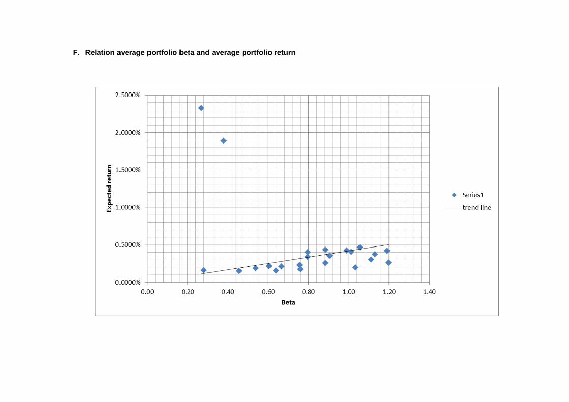
F. Relation average portfolio beta and average portfolio return
Recommended


![Examining CAPM in Today's Markets - [email protected]](https://img.pdfslide.us/doc/110x75/613d246b736caf36b759d09b/examining-capm-in-todays-markets-emailprotected.jpg)