Skyline queries Tecnologie delle Basi di Dati M
Limits of scoring functions
Although scoring functions are widely used to rank a set of objects, it is nowadays recognized that they have some major problems:
First, they have a limited expressive power, i.e., they can only capture
those user preferences that “translates into numbers”, which is not always the case (or, at least, doing so is not so natural!)
“I prefer having white wine with fish and red wine with meat”
Second, deciding on the “best” scoring function to use and/or the specific weights can be hardly left to the final user, especially when there are several ranking attributes
In this set of slides we will study an alternative to scoring functions, the so-called skyline queries, that have relevant practical applicability, and also represent a major step towards more general (i.e., powerful) preference models
Tecnologie delle Basi di Dati M 2

The concept of tuple domination
A fundamental concept underlying the definition of skyline queries is that of
The generalization to the case when the values of some attributes need to be maximized and to arbitrary target points is immediate
Tecnologie delle Basi di Dati M 3
Tuple domination: Given a relation R(A1,A2,…,Am,…), in which the Ai’s are ranking attributes,
assume without loss of generality that on each Ai lower values are better.
A tuple t dominates tuple t’ with respect to A = {A1,A2,…,Am}, written t ≻A t’ or simply t ≻ t’, iff:
j = 1,…,m: t.Aj t’.Aj j: t.Aj < t’.Aj
that is:
• t is no worse than t’ on all the attributes, and
• strictly better than t’ for at least one attribute
Notice that it can well be the case that neither t ≻ t’ nor t’ ≻ t hold
Tuple domination: example (1)
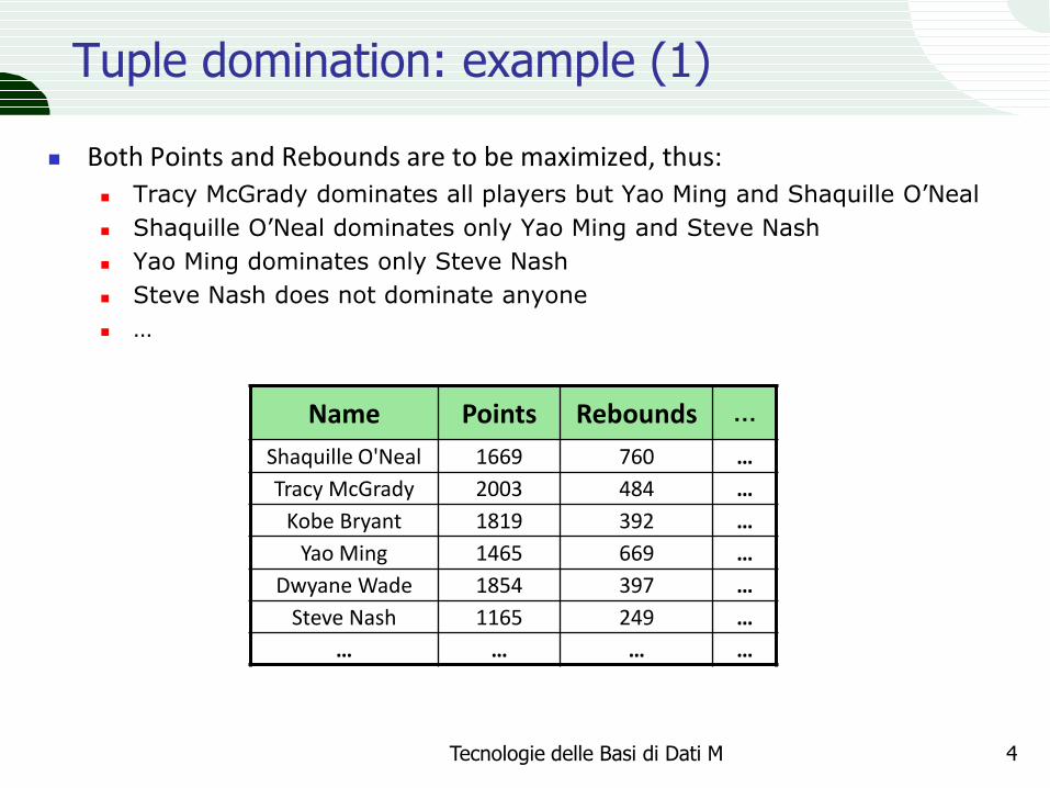
Both Points and Rebounds are to be maximized, thus: Tracy McGrady dominates all players but Yao Ming and Shaquille O’Neal
Shaquille O’Neal dominates only Yao Ming and Steve Nash
Yao Ming dominates only Steve Nash
Steve Nash does not dominate anyone
…
Tecnologie delle Basi di Dati M 4
Name Points Rebounds …
Shaquille O'Neal 1669 760 …
Tracy McGrady 2003 484 …
Kobe Bryant 1819 392 …
Yao Ming 1465 669 …
Dwyane Wade 1854 397 …
Steve Nash 1165 249 …
… … … …
Tuple domination: example (2)
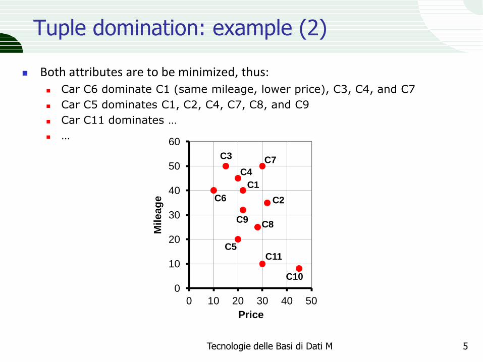
Both attributes are to be minimized, thus: Car C6 dominate C1 (same mileage, lower price), C3, C4, and C7
Car C5 dominates C1, C2, C4, C7, C8, and C9
Car C11 dominates …
…
Tecnologie delle Basi di Dati M 5
0
10
20
30
40
50
60
0 10 20 30 40 50
Mile
ag
e
Price
C1
C2
C3
C4
C5
C6
C7
C8 C9
C10
C11
Dominance region
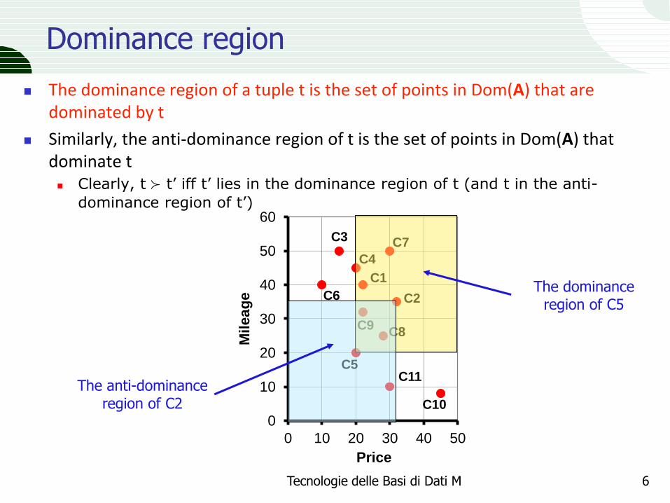
The dominance region of a tuple t is the set of points in Dom(A) that are dominated by t
Similarly, the anti-dominance region of t is the set of points in Dom(A) that dominate t Clearly, t ≻ t’ iff t’ lies in the dominance region of t (and t in the anti-
dominance region of t’)
Tecnologie delle Basi di Dati M 6
0
10
20
30
40
50
60
0 10 20 30 40 50
Mil
ea
ge
Price
C1
C2
C3
C4
C5
C6
C7
C8 C9
C10
C11
The dominance region of C5
The anti-dominance region of C2
The dominance graph
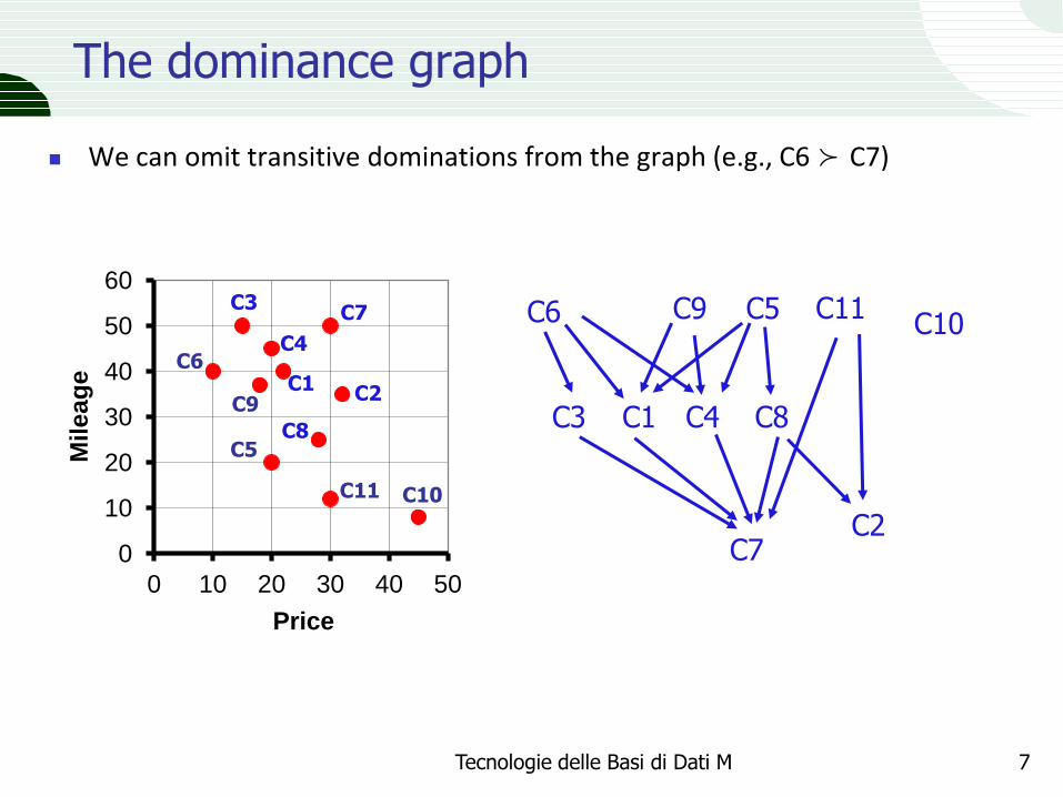
We can omit transitive dominations from the graph (e.g., C6 ≻ C7)
Tecnologie delle Basi di Dati M 7
0
10
20
30
40
50
60
0 10 20 30 40 50
Mile
ag
e
Price
C1 C2
C3
C4
C5
C6
C7
C8
C9
C10 C11
C5
C2
C3 C1 C4
C6
C8
C7
C10 C11 C9
Skyline queries
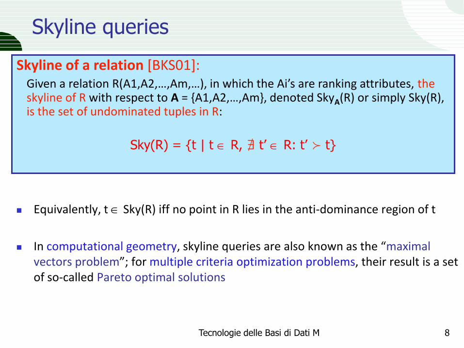
Equivalently, t Sky(R) iff no point in R lies in the anti-dominance region of t
In computational geometry, skyline queries are also known as the “maximal vectors problem”; for multiple criteria optimization problems, their result is a set of so-called Pareto optimal solutions
Tecnologie delle Basi di Dati M 8
Skyline of a relation [BKS01]: Given a relation R(A1,A2,…,Am,…), in which the Ai’s are ranking attributes, the
skyline of R with respect to A = {A1,A2,…,Am}, denoted SkyA(R) or simply Sky(R), is the set of undominated tuples in R:
Sky(R) = {t | t R, ∄ t’ R: t’ ≻ t}
A skyline example
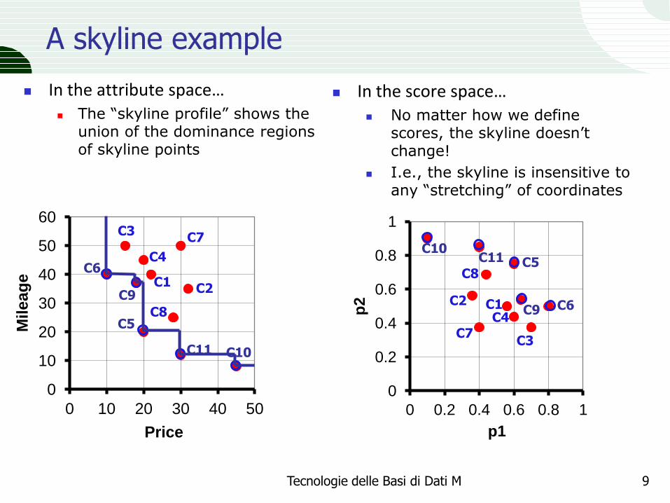
In the attribute space… The “skyline profile” shows the
union of the dominance regions of skyline points
Tecnologie delle Basi di Dati M 9
0
10
20
30
40
50
60
0 10 20 30 40 50
Mile
ag
e
Price
C1 C2
C3
C4
C5
C6
C7
C8
C9
C10 C11
0
0.2
0.4
0.6
0.8
1
0 0.2 0.4 0.6 0.8 1
p2
p1
C1 C2
C3
C4
C5
C6
C7
C8
C9
C10 C11
In the score space… No matter how we define
scores, the skyline doesn’t change!
I.e., the skyline is insensitive to any “stretching” of coordinates
What’s so special about skyline queries?
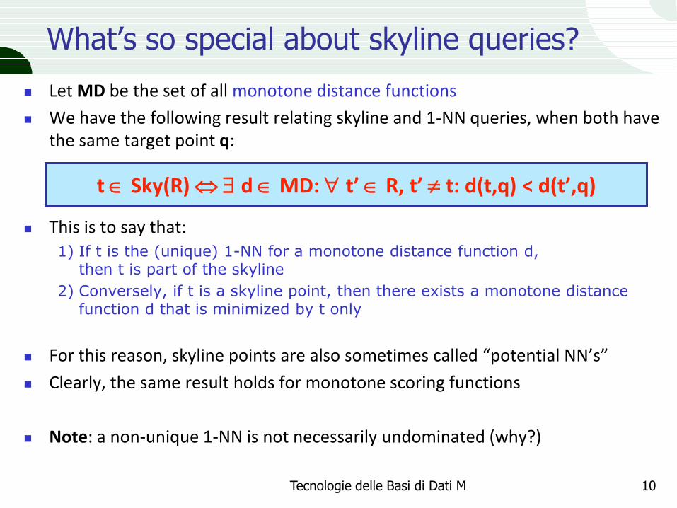
Let MD be the set of all monotone distance functions
We have the following result relating skyline and 1-NN queries, when both have the same target point q:
This is to say that: 1) If t is the (unique) 1-NN for a monotone distance function d,
then t is part of the skyline
2) Conversely, if t is a skyline point, then there exists a monotone distance function d that is minimized by t only
For this reason, skyline points are also sometimes called “potential NN’s”
Clearly, the same result holds for monotone scoring functions
Note: a non-unique 1-NN is not necessarily undominated (why?)
Tecnologie delle Basi di Dati M 10
t Sky(R) d MD: t’ R, t’ t: d(t,q) < d(t’,q)
Proof
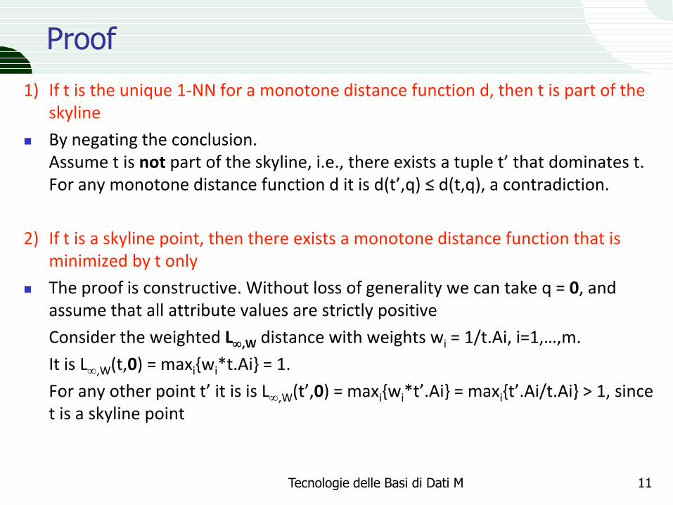
1) If t is the unique 1-NN for a monotone distance function d, then t is part of the skyline
By negating the conclusion. Assume t is not part of the skyline, i.e., there exists a tuple t’ that dominates t. For any monotone distance function d it is d(t’,q) ≤ d(t,q), a contradiction.
2) If t is a skyline point, then there exists a monotone distance function that is minimized by t only
The proof is constructive. Without loss of generality we can take q = 0, and assume that all attribute values are strictly positive
Consider the weighted L,W distance with weights wi = 1/t.Ai, i=1,…,m.
It is L,W(t,0) = maxi{wi*t.Ai} = 1.
For any other point t’ it is is L,W(t’,0) = maxi{wi*t’.Ai} = maxi{t’.Ai/t.Ai} > 1, since t is a skyline point
Tecnologie delle Basi di Dati M 11

“Accessibility” of skyline points
Tecnologie delle Basi di Dati M 12
Name Price Stars
Jolly 10 1
Rome 60 5
Paradise 40 3
S = Ws * Stars – Wp * Price
0
1
2
3
4
5
0 10 20 30 40 50 60
Sta
rs
Price
Jolly
Rome
Paradise
For no weights combination Paradise is the top-1 hotel
Similar problems with: Arbitrary values of k and/or
Almost all scoring functions
Hotels
Skylines do not admit any distance function
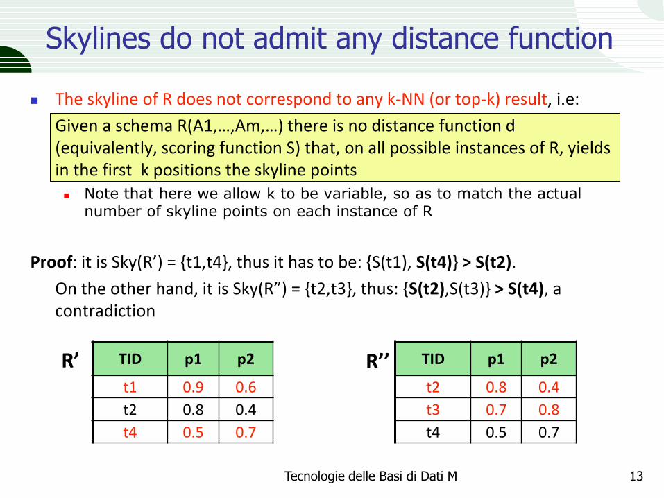
The skyline of R does not correspond to any k-NN (or top-k) result, i.e:
Given a schema R(A1,…,Am,…) there is no distance function d (equivalently, scoring function S) that, on all possible instances of R, yields in the first k positions the skyline points Note that here we allow k to be variable, so as to match the actual
number of skyline points on each instance of R
Proof: it is Sky(R’) = {t1,t4}, thus it has to be: {S(t1), S(t4)} > S(t2).
On the other hand, it is Sky(R”) = {t2,t3}, thus: {S(t2),S(t3)} > S(t4), a contradiction
Tecnologie delle Basi di Dati M 13
TID p1 p2
t1 0.9 0.6
t2 0.8 0.4
t4 0.5 0.7
TID p1 p2
t2 0.8 0.4
t3 0.7 0.8
t4 0.5 0.7
R’ R’’
Ranking with skylines
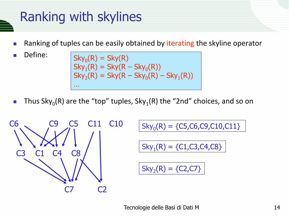
Ranking of tuples can be easily obtained by iterating the skyline operator
Define:
Thus Sky0(R) are the “top” tuples, Sky1(R) the “2nd” choices, and so on
Tecnologie delle Basi di Dati M 14
Sky0(R) = Sky(R) Sky1(R) = Sky(R – Sky0(R)) Sky2(R) = Sky(R – Sky0(R) – Sky1(R)) …
C5
C2
C3 C1 C4
C6
C8
C7
C10 C11 C9 Sky0(R) = {C5,C6,C9,C10,C11}
Sky1(R) = {C1,C3,C4,C8}
Sky2(R) = {C2,C7}
The issue of efficiently evaluating a skyline query has been largely investigated, and many algorithms introduced so far
A basic reason is that the problem is “more difficult” than top-k queries, since it has a worst-case complexity of (N2) for a DB with N objects
What we see are some algorithms that follow one of the two basic approaches:
Generic: it computes the skyline without any auxiliary access method (indexes) Thus, the input relation can also be the output of some other operation
(join, group by, etc.)
Index-based: it is assumed that an index is available
Tecnologie delle Basi di Dati M 15
Evaluation of skyline queries

The naïve Nested-Loops (NL) algorithm
The simplest (and very inefficient!) way to compute the skyline of R is to compare each tuple with all the others
Tecnologie delle Basi di Dati M 16
ALGORITHM NL (nested-loops)
Input: a dataset R, a set of attributes A inducing ≻
Output: Sky(R), the skyline of R with respect to A
1. Sky(R) := ;
2. for all tuples t in R:
3. undominated := true;
4. for all tuples t’ in R:
5. if t’ ≻ t then: {undominated := false; break}
6. if undominated then: Sky(R) := Sky(R) {t};
7. return Sky(R);
8. end.
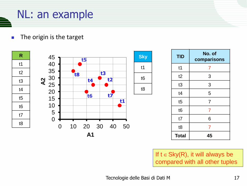
NL: an example
The origin is the target
Tecnologie delle Basi di Dati M 17
Sky
t1
t6
t8
0
5
10
15
20
25
30
35
40
45
0 10 20 30 40 50
A2
A1
t1
t2
t3
t4
t5
t6 t7
t8
R
t1
t2
t3
t4
t5
t6
t7
t8
TID No. of
comparisons
t1 7
t2 3
t3 3
t4 5
t5 7
t6 7
t7 6
t8 7
Total 45
If t Sky(R), it will always be
compared with all other tuples
The Block-Nested-Loops (BNL) algorithm
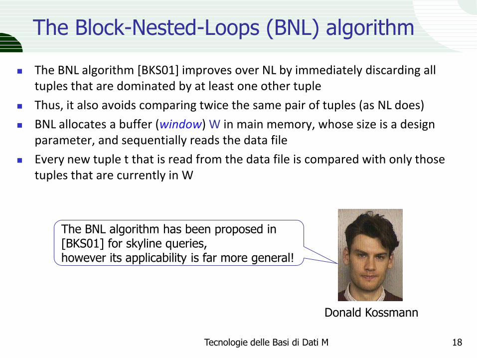
The BNL algorithm [BKS01] improves over NL by immediately discarding all tuples that are dominated by at least one other tuple
Thus, it also avoids comparing twice the same pair of tuples (as NL does)
BNL allocates a buffer (window) W in main memory, whose size is a design parameter, and sequentially reads the data file
Every new tuple t that is read from the data file is compared with only those tuples that are currently in W
Tecnologie delle Basi di Dati M 18
The BNL algorithm has been proposed in [BKS01] for skyline queries, however its applicability is far more general!
Donald Kossmann
The logic of the BNL algorithm
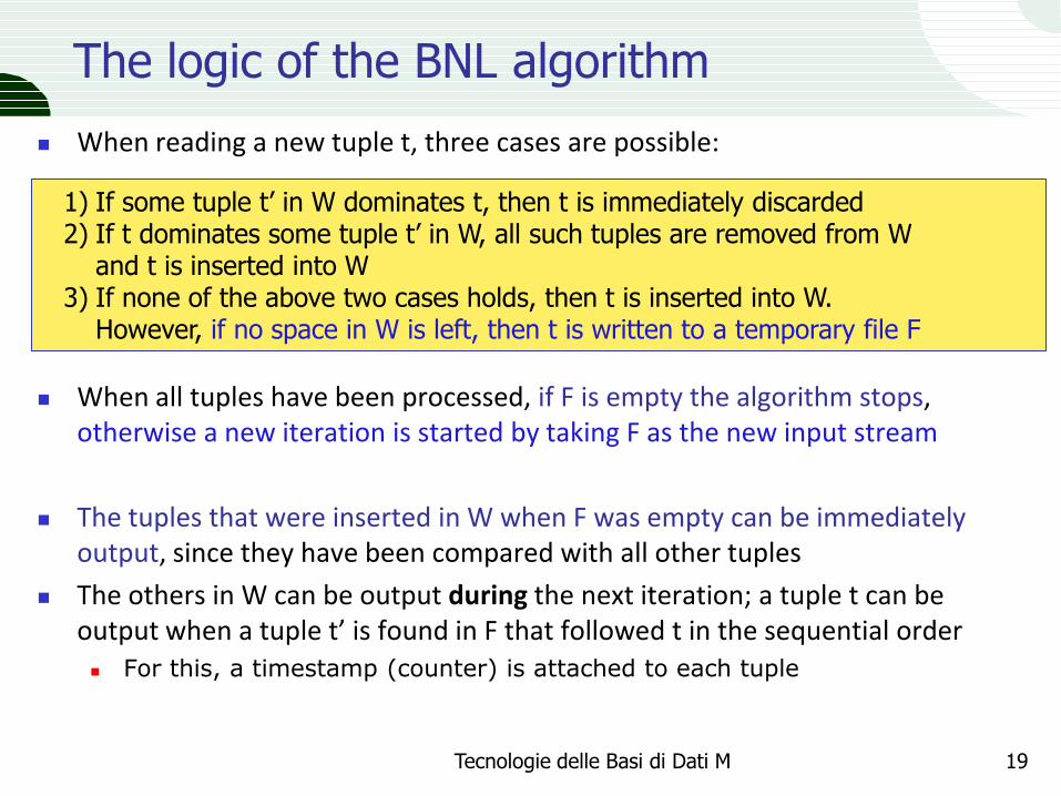
When reading a new tuple t, three cases are possible:
When all tuples have been processed, if F is empty the algorithm stops, otherwise a new iteration is started by taking F as the new input stream
The tuples that were inserted in W when F was empty can be immediately output, since they have been compared with all other tuples
The others in W can be output during the next iteration; a tuple t can be output when a tuple t’ is found in F that followed t in the sequential order For this, a timestamp (counter) is attached to each tuple
Tecnologie delle Basi di Dati M 19
1) If some tuple t’ in W dominates t, then t is immediately discarded 2) If t dominates some tuple t’ in W, all such tuples are removed from W
and t is inserted into W 3) If none of the above two cases holds, then t is inserted into W.
However, if no space in W is left, then t is written to a temporary file F
BNL: an example
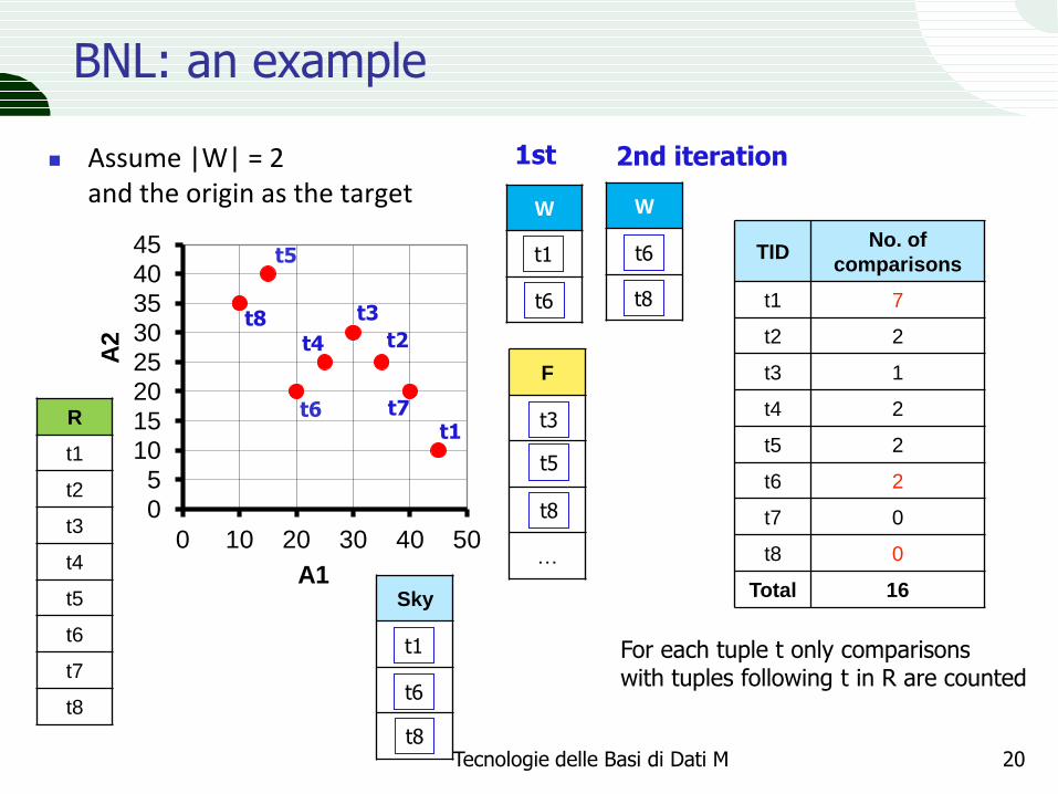
Assume |W| = 2 and the origin as the target
Tecnologie delle Basi di Dati M 20
W
t1
t2 t4
F
…
t3
t5
t6
t8
t1
W
t6
t5 t8
2nd iteration
t6
t8
0
5
10
15
20
25
30
35
40
45
0 10 20 30 40 50
A2
A1
t1
t2
t3
t4
t5
t6 t7
t8
R
t1
t2
t3
t4
t5
t6
t7
t8
TID No. of
comparisons
t1 7
t2 2
t3 1
t4 2
t5 2
t6 2
t7 0
t8 0
Total 16
1st
For each tuple t only comparisons with tuples following t in R are counted
Sky
21
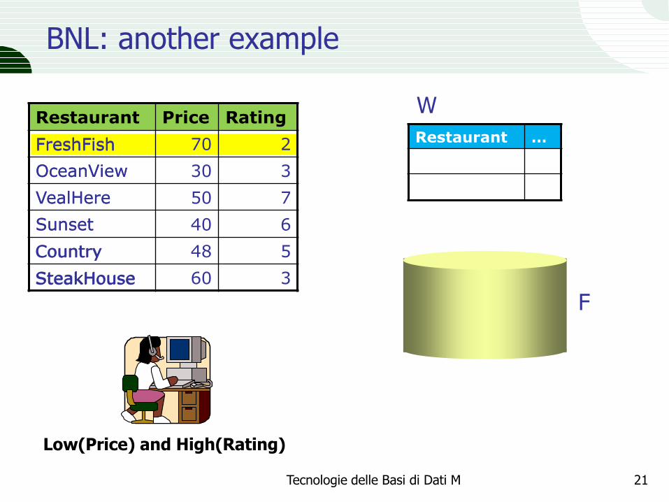
Restaurant Price Rating
FreshFish 70 2
OceanView 30 3
VealHere 50 7
Sunset 40 6
Country 48 5
SteakHouse 60 3
BNL: another example
Restaurant …
Low(Price) and High(Rating)
OceanView
FreshFish
Sunset
VealHere
Country
SteakHouse
W
Tecnologie delle Basi di Dati M
F
BNL: some comments
Experimental results in [BKS01] show that BNL is CPU-bound and that its performance deteriorates if W grows Since with larger W BNL executes more comparisons
On the other hand, BNL has a relatively low I/O cost
Performance is also negatively affected by the number of skyline points
The skyline cardinality depends on the number of attributes and on their correlation Negatively (or anti-)correlated attributes, like Price and Mileage, lead to
larger skylines
[BKS01] also introduces some variants of BNL, among which BNL-sol, that manages W as a self-organizing list The idea is to first compare incoming objects with those in W (called “killer”
objects) that have been found to dominate several other objects
… and another algorithm (D&C) based on a “divide-and-conquer” approach
Tecnologie delle Basi di Dati M 22
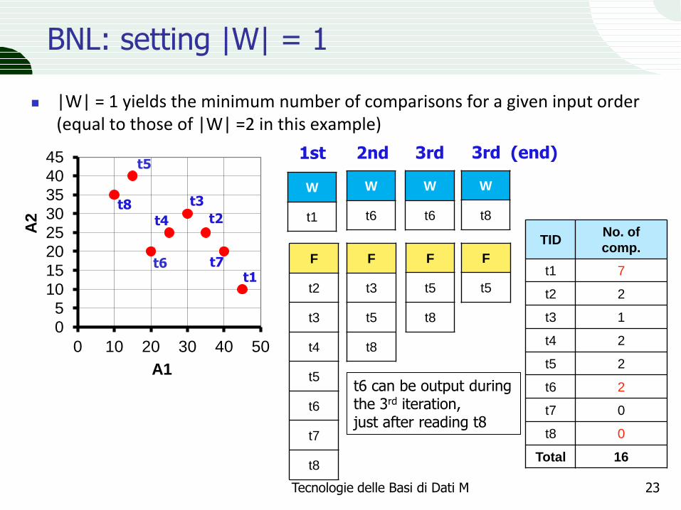
BNL: setting |W| = 1
|W| = 1 yields the minimum number of comparisons for a given input order (equal to those of |W| =2 in this example)
Tecnologie delle Basi di Dati M 23
W
t1
F
t2
t3
t4
t5
t6
t7
t8
W
t6
0
5
10
15
20
25
30
35
40
45
0 10 20 30 40 50
A2
A1
t1
t2
t3
t4
t5
t6 t7
t8
TID No. of
comp.
t1 7
t2 2
t3 1
t4 2
t5 2
t6 2
t7 0
t8 0
Total 16
F
t3
t5
t8
W
t6
F
t5
t8
W
t8
F
t5
1st 2nd 3rd 3rd (end)
t6 can be output during the 3rd iteration, just after reading t8
BNL: datasets and experiments (1) [BKS01]
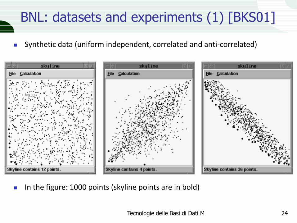
Synthetic data (uniform independent, correlated and anti-correlated)
In the figure: 1000 points (skyline points are in bold)
Tecnologie delle Basi di Dati M 24
BNL: datasets and experiments (2) [BKS01]
Tecnologie delle Basi di Dati M 25
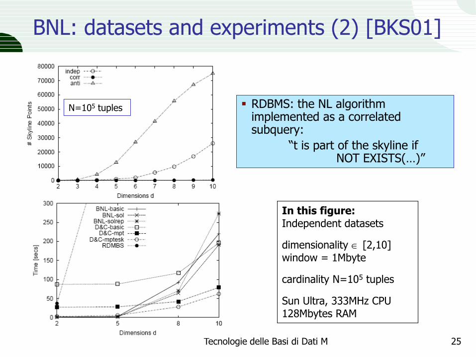
RDBMS: the NL algorithm implemented as a correlated subquery:
“t is part of the skyline if NOT EXISTS(…)”
In this figure: Independent datasets
dimensionality [2,10] window = 1Mbyte
cardinality N=105 tuples
Sun Ultra, 333MHz CPU 128Mbytes RAM
N=105 tuples
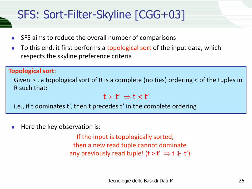
SFS: Sort-Filter-Skyline [CGG+03]
SFS aims to reduce the overall number of comparisons
To this end, it first performs a topological sort of the input data, which respects the skyline preference criteria
Here the key observation is:
If the input is topologically sorted, then a new read tuple cannot dominate
any previously read tuple! (t > t’ t ⊁ t’)
Tecnologie delle Basi di Dati M 26
Topological sort:
Given ≻, a topological sort of R is a complete (no ties) ordering < of the tuples in R such that:
t ≻ t’ t < t’
i.e., if t dominates t’, then t precedes t’ in the complete ordering
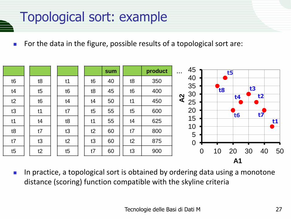
Topological sort: example
For the data in the figure, possible results of a topological sort are:
In practice, a topological sort is obtained by ordering data using a monotone distance (scoring) function compatible with the skyline criteria
Tecnologie delle Basi di Dati M 27
0
5
10
15
20
25
30
35
40
45
0 10 20 30 40 50
A2
A1
t1
t2
t3
t4
t5
t6 t7
t8
t6
t4
t2
t3
t1
t8
t7
t5
t8
t5
t6
t1
t4
t7
t3
t2
t1
t6
t4
t7
t8
t3
t2
t5
… sum
t6 40
t8 45
t4 50
t5 55
t1 55
t2 60
t3 60
t7 60
product
t8 350
t6 400
t1 450
t5 600
t4 625
t7 800
t2 875
t3 900
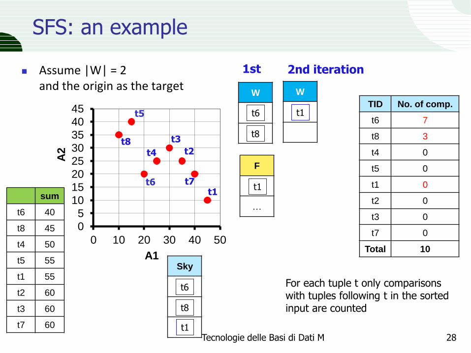
SFS: an example
Assume |W| = 2 and the origin as the target
Tecnologie delle Basi di Dati M 28
W
t6
t8
F
…
t1
t6
W
t1
2nd iteration
t8
t1
0
5
10
15
20
25
30
35
40
45
0 10 20 30 40 50
A2
A1
t1
t2
t3
t4
t5
t6 t7
t8
TID No. of comp.
t6 7
t8 3
t4 0
t5 0
t1 0
t2 0
t3 0
t7 0
Total 10
1st
For each tuple t only comparisons with tuples following t in the sorted input are counted
Sky
sum
t6 40
t8 45
t4 50
t5 55
t1 55
t2 60
t3 60
t7 60
SFS: further properties
At the end of each iteration all the tuples in W can be output since no tuple in W can be discarded by a subsequent tuple
The number of iterations is therefore the minimum one: |Sky(R)|/|W| In contrast, BNL has no such guarantee
SFS can return a tuple as soon as it is inserted in the window Therefore, in W one can just store the skyiline attribute values, which
leads to save (much) space
Two non-skyline tuples will never be compared Since in W only skyline tuples are present
Managing the window data structure is now much easier Since only insertions are to be supported
No deletion of specific tuples, thus no need to manage empty slots
Tecnologie delle Basi di Dati M 29

Experimental results (from [CGG+03])
Data sorted using the “entropy” distance function:
d(t,0) = - i=1,m ln(2 - t.Ai)
= - ln(exp(i=1,m ln(2 - t.Ai))) = - ln ( i=1,m(2-t.Ai) )
which yields the same ordering as 2m - i=1,m(2-t.Ai) ( [0,2m – 1])
Tecnologie delle Basi di Dati M 30
BNL w/RE: input sorted using the “reverse” entropy
Independent dataset cardinality N=106 tuples dimensionality = 7 window = # 4Kbyte pages AMD Athlon, 900MHz CPU 384Mbytes RAM
SaLSa [BCP06,BCP08]
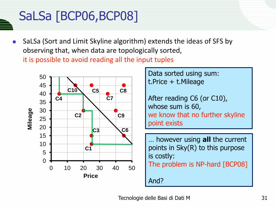
SaLSa (Sort and Limit Skyline algorithm) extends the ideas of SFS by observing that, when data are topologically sorted, it is possible to avoid reading all the input tuples
Tecnologie delle Basi di Dati M 31
0
5
10
15
20
25
30
35
40
45
50
0 10 20 30 40 50
Mile
ag
e
Price
C1
C2
C3
C4
C5
C6
C7
C8
C9
C10
Data sorted using sum: t.Price + t.Mileage After reading C6 (or C10), whose sum is 60, we know that no further skyline point exists
… however using all the current points in Sky(R) to this purpose is costly: The problem is NP-hard [BCP08] And?

The “stop-point”
SaLSa makes use of a single skyline tuple, the so-called stop-point , tstop, to determine when execution can be halted
In this case it is sufficient to check that what is still to be read lies in the dominance region of tstop
Tecnologie delle Basi di Dati M 32
0
5
10
15
20
25
30
35
40
45
50
0 10 20 30 40 50
Mile
ag
e
Price
C1
C2
C3
C4
C5
C6
C7
C8
C9
C10
tstop
halt when
sum ≥
C1 75
C2 80
C4 90 75
80
90
Choosing the stop-point
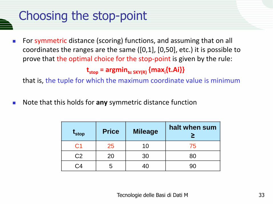
For symmetric distance (scoring) functions, and assuming that on all coordinates the ranges are the same ([0,1], [0,50], etc.) it is possible to prove that the optimal choice for the stop-point is given by the rule:
tstop = argmintSKY(R) {maxi{t.Ai}}
that is, the tuple for which the maximum coordinate value is minimum
Note that this holds for any symmetric distance function
Tecnologie delle Basi di Dati M 33
tstop Price Mileage
halt when sum
≥
C1 25 10 75
C2 20 30 80
C4 5 40 90
Optimally ordering the points
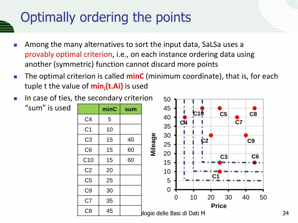
Among the many alternatives to sort the input data, SaLSa uses a provably optimal criterion, i.e., on each instance ordering data using another (symmetric) function cannot discard more points
The optimal criterion is called minC (minimum coordinate), that is, for each tuple t the value of mini{t.Ai} is used
In case of ties, the secondary criterion “sum” is used
Tecnologie delle Basi di Dati M 34
0
5
10
15
20
25
30
35
40
45
50
0 10 20 30 40 50
Mile
ag
e
Price
C1
C2
C3
C4
C5
C6
C7
C8
C9
C10 minC sum
C4 5
C1 10
C3 15 40
C6 15 60
C10 15 60
C2 20
C5 25
C9 30
C7 35
C8 45
Stopping with minC
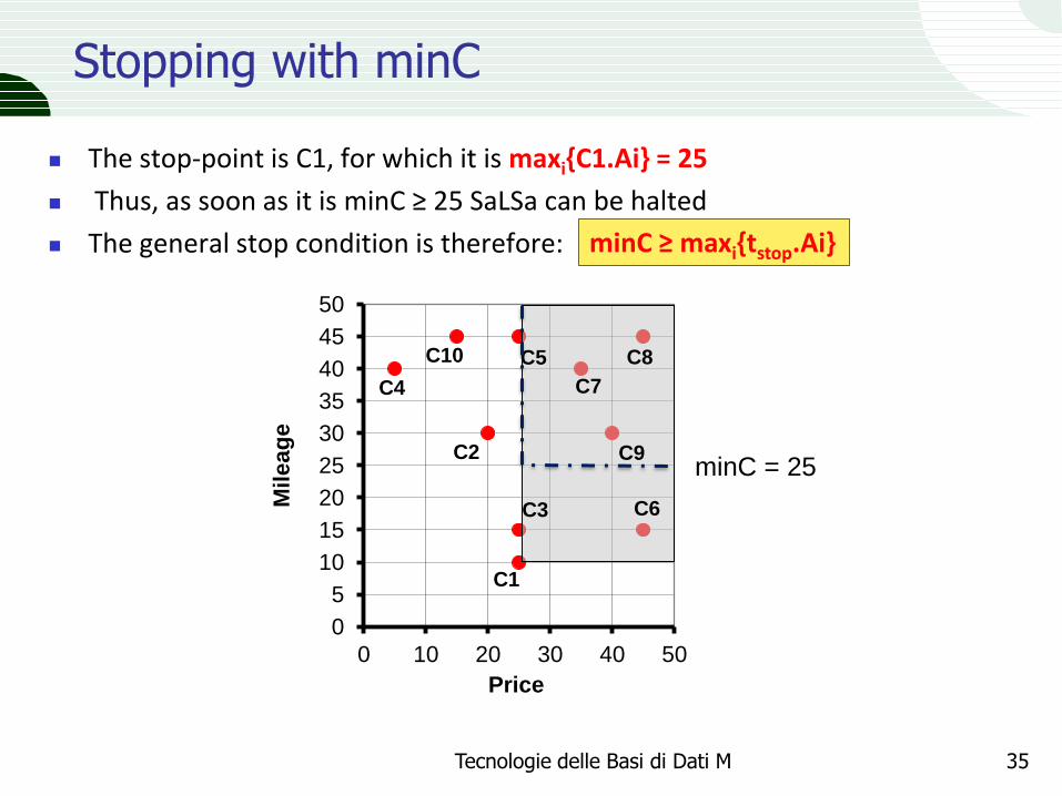
The stop-point is C1, for which it is maxi{C1.Ai} = 25
Thus, as soon as it is minC ≥ 25 SaLSa can be halted
The general stop condition is therefore:
Tecnologie delle Basi di Dati M 35
0
5
10
15
20
25
30
35
40
45
50
0 10 20 30 40 50
Mile
ag
e
Price
C1
C2
C3
C4
C5
C6
C7
C8
C9
C10
minC ≥ maxi{tstop.Ai}
minC = 25

Experimental results (from [BCP08]) (1)
FP = fraction of fetched points, independent datasets (vol = SFS)
Tecnologie delle Basi di Dati M 36
cardinality N [105,5*105] tuples dimensionality = 4
cardinality N=5*105 tuples dimensionality [2,6]
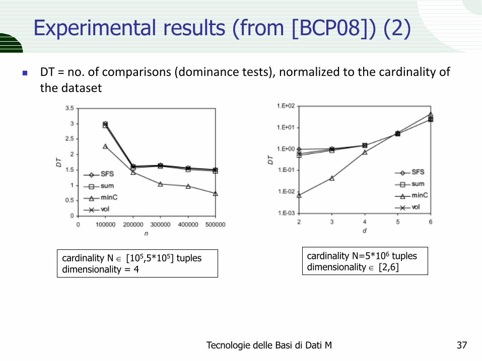
Experimental results (from [BCP08]) (2)
DT = no. of comparisons (dominance tests), normalized to the cardinality of the dataset
Tecnologie delle Basi di Dati M 37
cardinality N [105,5*105] tuples dimensionality = 4
cardinality N=5*106 tuples dimensionality [2,6]
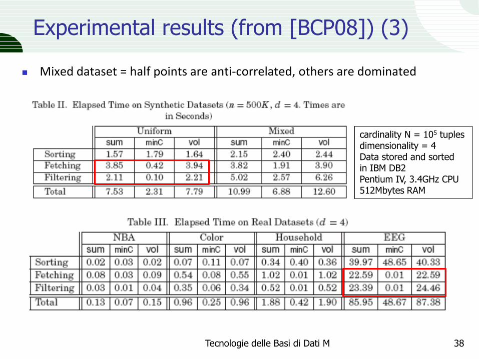
Experimental results (from [BCP08]) (3)
Mixed dataset = half points are anti-correlated, others are dominated
Tecnologie delle Basi di Dati M 38
cardinality N = 105 tuples dimensionality = 4 Data stored and sorted in IBM DB2 Pentium IV, 3.4GHz CPU 512Mbytes RAM
Computing the skyline with R-trees
If we have an index over the ranking attributes, we can use it to avoid scanning the whole DB
The BBS (Branch and Bound Skyline) algorithm [PTF+03] is reminiscent of kNNOptimal, in that it accesses index nodes by increasing values of MinDist (in the following the query/target point coincides with the origin) and of next-NN, in that the queue PQ keeps both tuples and nodes For computational economy, [PTF+03] evaluates distances using L1
(Manhattan distance)
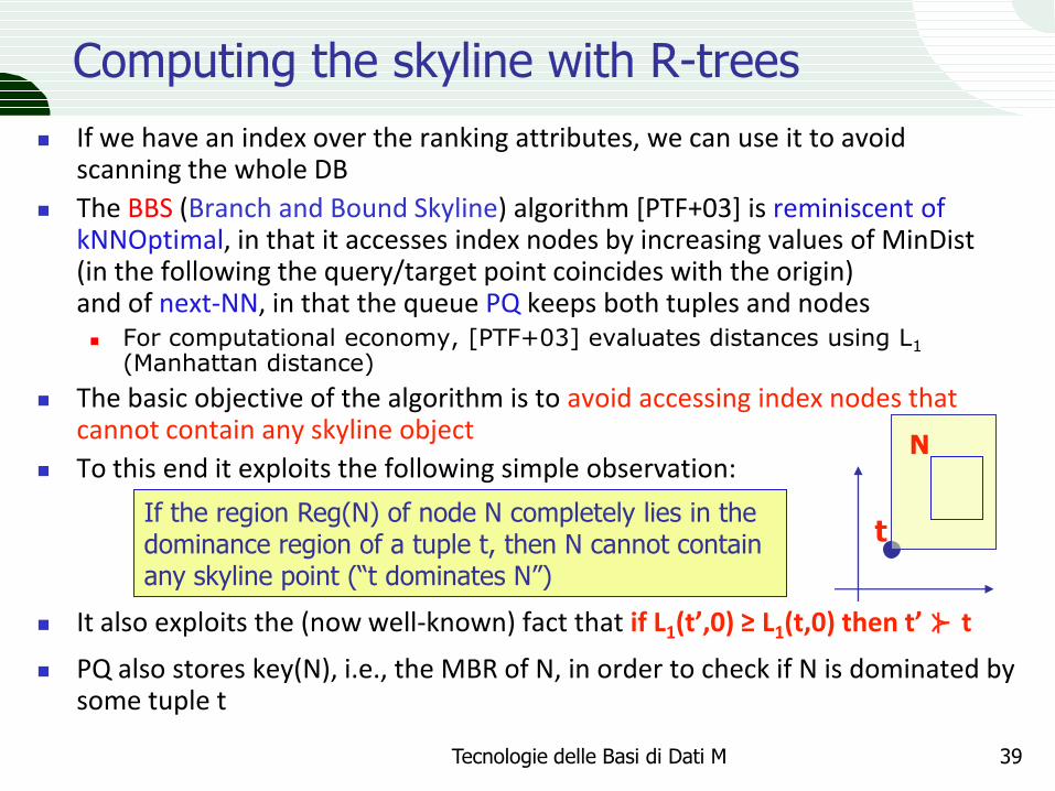
The basic objective of the algorithm is to avoid accessing index nodes that cannot contain any skyline object
To this end it exploits the following simple observation:
It also exploits the (now well-known) fact that if L1(t’,0) ≥ L1(t,0) then t’ ⊁ t
PQ also stores key(N), i.e., the MBR of N, in order to check if N is dominated by some tuple t
Tecnologie delle Basi di Dati M 39
If the region Reg(N) of node N completely lies in the dominance region of a tuple t, then N cannot contain any skyline point (“t dominates N”)
t
N
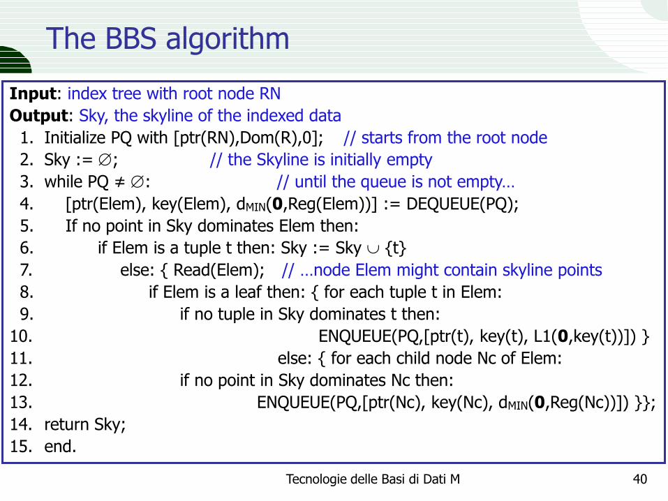
The BBS algorithm
Tecnologie delle Basi di Dati M 40
Input: index tree with root node RN
Output: Sky, the skyline of the indexed data
1. Initialize PQ with [ptr(RN),Dom(R),0]; // starts from the root node
2. Sky := ; // the Skyline is initially empty
3. while PQ ≠ : // until the queue is not empty…
4. [ptr(Elem), key(Elem), dMIN(0,Reg(Elem))] := DEQUEUE(PQ);
5. If no point in Sky dominates Elem then:
6. if Elem is a tuple t then: Sky := Sky {t}
7. else: { Read(Elem); // …node Elem might contain skyline points
8. if Elem is a leaf then: { for each tuple t in Elem:
9. if no tuple in Sky dominates t then:
10. ENQUEUE(PQ,[ptr(t), key(t), L1(0,key(t))]) }
11. else: { for each child node Nc of Elem:
12. if no point in Sky dominates Nc then:
13. ENQUEUE(PQ,[ptr(Nc), key(Nc), dMIN(0,Reg(Nc))]) }};
14. return Sky;
15. end.
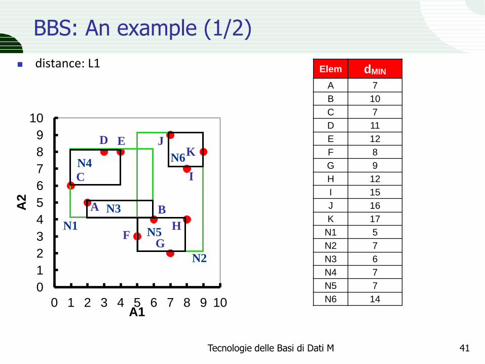
BBS: An example (1/2)
distance: L1
Tecnologie delle Basi di Dati M 41
0
1
2
3
4
5
6
7
8
9
10
0 1 2 3 4 5 6 7 8 9 10
A2
A1
N1
A
Elem dMIN
A 7
B 10
C 7
D 11
E 12
F 8
G 9
H 12
I 15
J 16
K 17
N1 5
N2 7
N3 6
N4 7
N5 7
N6 14
B
C
D E
F G
H
I
J K
N2
N3
N4
N5
N6
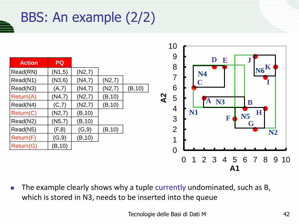
BBS: An example (2/2)
The example clearly shows why a tuple currently undominated, such as B, which is stored in N3, needs to be inserted into the queue
Tecnologie delle Basi di Dati M 42
Action PQ
Read(RN) (N1,5) (N2,7)
Read(N1) (N3,6) (N4,7) (N2,7)
Read(N3) (A,7) (N4,7) (N2,7) (B,10)
Return(A) (N4,7) (N2,7) (B,10)
Read(N4) (C,7) (N2,7) (B,10)
Return(C) (N2,7) (B,10)
Read(N2) (N5,7) (B,10)
Read(N5) (F,8) (G,9) (B,10)
Return(F) (G,9) (B,10)
Return(G) (B,10) 0
1
2
3
4
5
6
7
8
9
10
0 1 2 3 4 5 6 7 8 9 10 A
2
A1
N1
A B
C
D E
F G
H
I
J K
N2
N3
N4
N5
N6
Tecnologie delle Basi di Dati M 43
NN BBS
1e+0
1e+1
1e+2
1e+3
1e+4
1e+5
1e+6
1e+7
2 3 4 5
dimensionality
node accesses
1e+0
1e+1
1e+2
1e+3
1e+4
1e+5
1e+6
1e+7
2 3 4 5
dimensionality
node accesses
Independent Anti-correlated
Node accesses vs. d (N=1M)
CPU time (secs)
dimensionality0
1e-2
1e-1
1e+0
1e+1
1e+2
1e+3
2 3 4 5 1e-3
1e-2
1e-1
1e+0
1e+1
1e+2
1e+3
1e+4
2 3 4 5
dimensionality
CPU time (secs)
Independent Anti-correlated
CPU-time vs. d (N=1M)
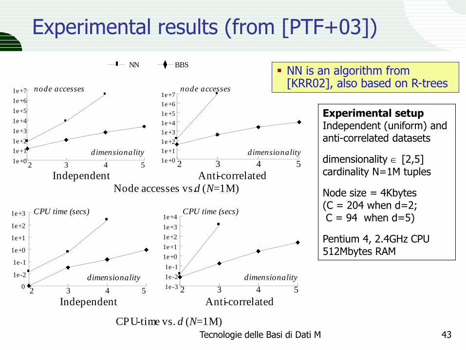
NN is an algorithm from [KRR02], also based on R-trees
Experimental setup Independent (uniform) and anti-correlated datasets
dimensionality [2,5] cardinality N=1M tuples
Node size = 4Kbytes (C = 204 when d=2; C = 94 when d=5)
Pentium 4, 2.4GHz CPU 512Mbytes RAM
Experimental results (from [PTF+03])
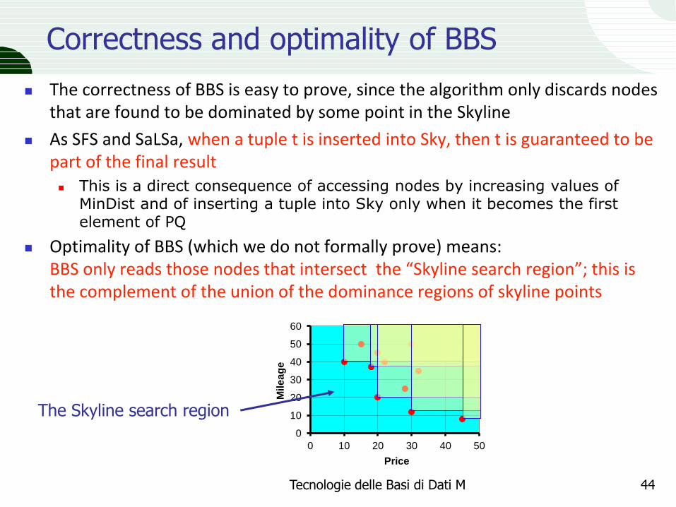
Correctness and optimality of BBS
The correctness of BBS is easy to prove, since the algorithm only discards nodes that are found to be dominated by some point in the Skyline
As SFS and SaLSa, when a tuple t is inserted into Sky, then t is guaranteed to be part of the final result This is a direct consequence of accessing nodes by increasing values of
MinDist and of inserting a tuple into Sky only when it becomes the first element of PQ
Optimality of BBS (which we do not formally prove) means: BBS only reads those nodes that intersect the “Skyline search region”; this is the complement of the union of the dominance regions of skyline points
Tecnologie delle Basi di Dati M 44
0
10
20
30
40
50
60
0 10 20 30 40 50
Mile
ag
e
Price
The Skyline search region
Skylines for low-cardinality domains
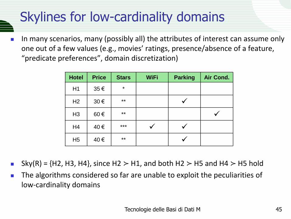
In many scenarios, many (possibly all) the attributes of interest can assume only one out of a few values (e.g., movies’ ratings, presence/absence of a feature, “predicate preferences”, domain discretization)
Sky(R) = {H2, H3, H4}, since H2 ≻ H1, and both H2 ≻ H5 and H4 ≻ H5 hold
The algorithms considered so far are unable to exploit the peculiarities of low-cardinality domains
Tecnologie delle Basi di Dati M 45
Hotel Price Stars WiFi Parking Air Cond.
H1 35 € *
H2 30 € **
H3 60 € **
H4 40 € ***
H5 40 € **
LS-B: all attributes have low cardinality
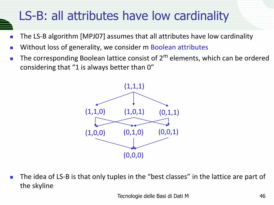
The LS-B algorithm [MPJ07] assumes that all attributes have low cardinality
Without loss of generality, we consider m Boolean attributes
The corresponding Boolean lattice consist of 2m elements, which can be ordered considering that “1 is always better than 0”
The idea of LS-B is that only tuples in the “best classes” in the lattice are part of the skyline
Tecnologie delle Basi di Dati M 46
(1,1,0)
(1,0,0)
(0,0,0)
(1,0,1)
(0,1,0) (0,0,1)
(0,1,1)
(1,1,1)
The LS-B algorithm
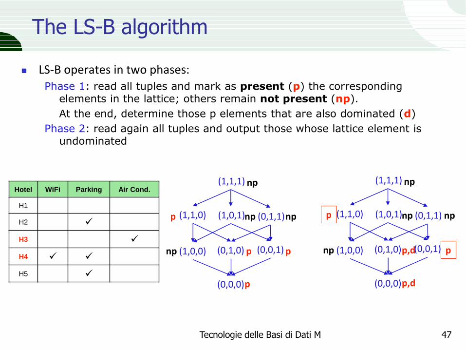
LS-B operates in two phases: Phase 1: read all tuples and mark as present (p) the corresponding
elements in the lattice; others remain not present (np).
At the end, determine those p elements that are also dominated (d)
Phase 2: read again all tuples and output those whose lattice element is undominated
Tecnologie delle Basi di Dati M 47
Hotel WiFi Parking Air Cond.
H1
H2
H3
H4
H5
(1,1,0)
(1,0,0)
(0,0,0)
(1,0,1)
(0,1,0) (0,0,1)
(0,1,1)
(1,1,1) np
np
p
p p np
p np (1,1,0)
(1,0,0)
(0,0,0)
(1,0,1)
(0,1,0) (0,0,1)
(0,1,1)
(1,1,1) np
np
p,d
p p,d np
p np
LS: all attributes but one have low cardinality
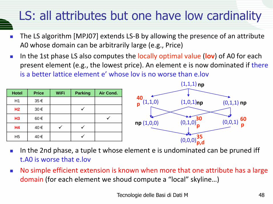
The LS algorithm [MPJ07] extends LS-B by allowing the presence of an attribute A0 whose domain can be arbitrarily large (e.g., Price)
In the 1st phase LS also computes the locally optimal value (lov) of A0 for each present element (e.g., the lowest price). An element e is now dominated if there is a better lattice element e’ whose lov is no worse than e.lov
In the 2nd phase, a tuple t whose element e is undominated can be pruned iff t.A0 is worse that e.lov
No simple efficient extension is known when more that one attribute has a large domain (for each element we shoud compute a “local” skyline…)
Tecnologie delle Basi di Dati M 48
Hotel Price WiFi Parking Air Cond.
H1 35 €
H2 30 €
H3 60 €
H4 40 €
H5 40 €
(1,1,0)
(1,0,0)
(0,0,0)
(1,0,1)
(0,1,0) (0,0,1)
(0,1,1)
(1,1,1) np
np
p,d
p p np
p np 40
60 30
35
Variants of skyline queries
[PTF+03] introduces some variants of basic skyline queries:
Many other skyline-related problems have been proposed/studied so far, e.g.: Reverse skyline queries: given a query point q, which are the tuples t such
that q is in the skyline computed with respect to t (when t is the target)?
Representative skyline points: which are the k “most representative” points in the skyline?
See [CCM13] for a recent survey on the subject
Tecnologie delle Basi di Dati M 49
1. Ranked skyline queries ranking within the skyline with a scoring function
2. Constrained skyline queries limiting the search region
3. K-dominating queries the k tuples that dominate the largest number of other tuples
Dimitris Papadias
Summary on skyline queries
Skyline queries represent a valid alternative to top-k queries, since they do not require any choice of scoring functions and weights
The skyline of a relation R, Sky(R), contains all and only the undominated tuples in R, i.e., those tuples representing “interesting alternatives” to consider
Computing Sky(R) can rely on both sequential and index-based algorithms
The BNL algorithm works by allocating a main-memory window, and then comparing incoming tuples with those in the window
SFS pre-sorts data yielding a topological sort that introduces several benefits compared to BNL
SaLSa adds a stop condition, that avoids reading all the data
BBS is a provably I/O-optimal algorithm for computing Sky(R) using an R-tree
LS-B and LS are designed to work with low-cardinality domains (and at most one large attribute domain)
Tecnologie delle Basi di Dati M 50
References
[BCP06] Ilaria Bartolini, Paolo Ciaccia, Marco Patella: SaLSa: computing the skyline without scanning the whole sky. CIKM 2006: 405-414
[BCP08] Ilaria Bartolini, Paolo Ciaccia, Marco Patella: Efficient sort-based skyline evaluation. ACM Trans. Database Syst. 33(4): (2008)
[BKS01] Stephan Börzsönyi, Donald Kossmann, Konrad Stocker: The Skyline Operator. ICDE 2001: 421-430
[CCM13] Jan Chomicki, Paolo Ciaccia, Niccolò Meneghetti: Skyline Queries, Front and Back. SIGMOD RECORD 2013: 6-18
[CGG+03] Jan Chomicki, Parke Godfrey, Jarek Gryz, Dongming Liang: Skyline with Presorting. ICDE 2003: 717-719
[KRR02] Donald Kossmann, Frank Ramsak, Steffen Rost: Shooting Stars in the Sky: An Online Algorithm for Skyline Queries. VLDB 2002: 275-286
[MPJ07] Michael D. Morse, Jignesh M. Patel, H. V. Jagadish: Efficient Skyline Computation over Low-Cardinality Domains. VLDB 2007: 267-278
[PTF+03] Dimitris Papadias, Yufei Tao, Greg Fu, Bernhard Seeger: An Optimal and Progressive Algorithm for Skyline Queries. SIGMOD Conference 2003: 467-478
Tecnologie delle Basi di Dati M 51
Recommended