Technological Change and Reallocation∗
Junghoon Lee†
September 14, 2017
Abstract
This paper considers a technological change that can be utilized only
by production units adapting to new technology. A simple firm dynam-
ics model is used to show how such an innovation enhances reallocation,
whereas a technological advance that is available to all production units
does not. This implication is used in structural vector autoregressions
to study the driving force behind cyclical movements in reallocation and
the rival/nonrival nature of technology. This paper finds that one sin-
gle shock explains most of the unpredictable movements in reallocation
over a three- to ten-year horizon and that this shock is closely related
to the investment-specific technology shock identified by long-run re-
strictions. The investment-specific technology shock also accounts for
more than 35 percent of hours forecast errors over a two- to ten-year
horizon. These findings imply that technology shocks responsible for a
large portion of economic fluctuations are the main driving force behind
cyclical variations in reallocation, confirming a rival or Schumpeterian
nature of technological progress.
∗I thank R. Anton Braun, Thorsten Drautzburg, Shigeru Fujita, Andre Kurmann, B.Ravikumar, Harald Uhlig, Tao Zha, and especially Steven J. Davis for their helpful commentsand suggestions. All remaining errors are my own.†Department of Economics, Emory University, 1602 Fishburne Drive, Atlanta, GA 30322,
USA. Email: [email protected].
1

1 Introduction
This paper seeks to answer the following questions. What types of shocks
drive cyclical movements in reallocation? What do fluctuations in reallocation
tell us about the nature—rival or nonrival—of technological change?
Reallocation is a pervasive feature of market economies.1 Reallocation also
accounts for a large portion of productivity growth2 and the pace of realloca-
tion varies considerably over time.3 These facts have motivated many studies
to investigate the role of reallocation shocks.4
Whether technology is rival or nonrival has also received a lot of attention
in the literature (see Acemoglu, 2009). The standard Solow and neoclassical
growth models assume that technology is a nonrival good: once a new tech-
nology is developed, it can be used by any producer without precluding its
use by others. In contrast, the Schumpeterian growth models (e.g., Aghion
and Howitt, 1992) feature the rival nature of technology so that a technologi-
cal innovation can be utilized only by some producers that adapt to the new
knowledge.5
1For example, Davis and Haltiwanger (1999a) document that more than one in ten jobsis either created or destroyed every year in the U.S. Baldwin et al. (1993) show that entryand exit accounts for about 40 percent of job creation and destruction over a five-year span inthe U.S. and Canada manufacturing sectors between 1972 and 1982. Eisfeldt and Rampini(2006) report that the reallocation of existing capital of publicly traded firms comprisesabout one quarter of the U.S. total investment from 1971 to 2000.
2Foster et al. (2001), for example, find that over 50 percent of productivity growth inthe U.S. manufacturing sector between 1977 and 1987 is attributed to reallocation; entryand exit in turn account for half of this contribution.
3Davis and Haltiwanger (1999a) document that the job destruction rate ranges from 2.9percent to 10.8 percent per quarter, while the job creation rate ranges from 3.8 percent to10.2 percent for the U.S. manufacturing sector from 1947:I to 1993:IV.
4To name a few, Lilien (1982), Abraham and Katz (1986), and Blanchard and Diamond(1989) are early contributions to this large literature.
5Hence, like these different strands of the growth literature, I broadly interpret therival/nonrival nature of technology as including all factors affecting the ease of technologyadoption rather than the intrinsic nature of technology per se.
2

This paper addresses the two questions above jointly by finding a strong
link between technology shocks and reallocation shocks. By reallocation shocks,
I mean shocks that account for the most variation in reallocation. I show that
investment-specific technology shocks account for over 50 percent of all un-
predictable movements in reallocation over a four- to ten-year horizon. These
results hold for various reallocation measures over the period 1993-2014; i.e,
establishment turnover (entry plus exit) rates, job reallocation (creation plus
destruction) rates, and capital turnover rates. Hence, investment-specific tech-
nology shocks are the main driving force behind cyclical movements in reallo-
cation.
My findings also reveal the rival nature of investment-specific technology.
If new technology is nonrival and readily available, all production units can
avoid becoming obsolete and aggregate productivity can grow without the need
for restructuring. Technological progress entails incessant reallocation only
when new knowledge is rival, thereby involving the replacement of outdated
units by new ones. Hours worked rise gradually after an investment-specific
technology shock, which explains more than 35 percent of the unpredictable
variations in hours over a two- to ten-year horizon.6 Therefore, technology
shocks responsible for a large portion of aggregate fluctuations are rival and
disruptive, leading to increased reallocation.
In sum, this paper finds that technological progress fostering ongoing real-
location is a major driver of economic fluctuations. This finding confirms the
importance of Schumpeterian creative destruction for reallocation and macroe-
conomic fluctuations.
6These findings are consistent with the business cycle literature documenting investment-specific technological change as a major source of business cycle fluctuations (e.g., Green-wood et al., 2000; Fisher, 2006; Justiniano et al., 2010).
3

My analysis starts by constructing a simple firm dynamics model and
demonstrates the different impact of various types of technological change on
reallocation. The economy consists of plants and potential entrants. Plants
produce aggregate output with their plant-specific productivity and can exit
the market by selling off their capital. Potential entrants are those who possess
new technology and they can build new plants by purchasing capital goods.
There are four types of technology shocks. First, nonrival investment-neutral
technology shocks enhance the productivity of all plants. Second, nonrival
investment-specific technology shocks lower the price of capital goods traded
by all plants. Third, rival investment-neutral technology shocks increase the
average productivity level of new technology (e.g., new skills or organization)
that can be implemented by startups only. Finally, rival investment-specific
technology shocks improve the efficiency of new vintage capital. The second
and fourth types of shocks lower the quality-adjusted price of capital. The lat-
ter two types of technology are distinctive in that they can be taken advantage
of by entrants only and not by all production units.
All four types of shocks in this economy encourage entry and result in an
economic boom. However, only the third and fourth types—both of which are
rival technology shocks—increase exit as well. Only new plants become more
productive and the widened productivity gap between entrants and incumbents
makes old plants less valuable in production. In contrast, the other two types
of shocks do not encourage exit because they affect new and old plants equally.
I then consider a vector autoregression (VAR) that combines reallocation
variables with standard macroeconomic aggregates. I first identify a realloca-
tion shock as one that accounts for most of the forecast error variance (FEV) of
the reallocation rate over the business cycle horizon.7 This data-driven iden-
7This identification of the reallocation shock is different from previous works, which
4

tification quantitatively uncovers the most important shock for reallocation
but does not offer any economic interpretation. I then interpret this shock
by examining its impulse responses through the lens of the theoretical model.
The responses of entry/exit, job creation/destruction, and capital reallocation
to this reallocation shock are similar to what is seen in the rival technology
shock in my firm dynamics model.
The identified reallocation shock accounts for over 50 to 75 percent of all
unpredictable fluctuations in reallocation over a three- to ten-year horizon.
This shock persistently lowers the quality-adjusted price of capital goods. It is
then compared to the investment-specific technology shock identified by long-
run restrictions in the manner of Fisher (2006), which is the only shock to
have a long-run effect on the capital goods price. I find that these two shocks
are highly correlated with a correlation coefficient larger than 85 percent and
their estimated impulse responses are also very similar. This finding suggests
that the investment-specific technology shocks featured in the business cycle
literature are the main driving force behind cyclical movements in reallocation
and that this Schumpeterian or disruptive technological change is a major
source of business cycle fluctuations.
1.1 Related Literature
The cyclicality of reallocation has been studied in many previous works. For
example, Davis and Haltiwanger (1992) and Davis et al. (2006) document con-
typically identify the reallocation shock as the shock orthogonal to the aggregate shock (see,for example, Blanchard and Diamond, 1989; Davis and Haltiwanger, 1999b; Caballero andHammour, 2005). In other words, previous studies extract the shock affecting the remainingvariations in reallocation after controlling for the effect of aggregate activity (expansion orcontraction) on the reallocation, whereas the reallocation shock in this study achieves themaximal variation in reallocation.
5

tercyclical fluctuations in job reallocation and Campbell (1998) reports that
the entry rate is procyclical, whereas the exit rate is countercyclical. These
studies, however, are based on unconditional correlations and are not contra-
dictory to my findings that the job reallocation and establishment turnover
rates rise conditional on expansionary technology shocks.8 My time-series re-
sults are also in line with the cross-section results of Samaniego (2009), who
finds that industry turnover rates are positively related to the industry rates
of investment-specific technological change.
Ravn and Simonelli (2007), Balleer (2012), and Canova et al. (2013) also
use long-run restrictions in VAR9 to study the effects of technology shocks
on labor market dynamics. These authors are, however, motivated by search
models and analyze cyclical movements in worker flow such as job finding
and separation rates. In contrast, this paper is interested in the effects of
technological progress on restructuring production units, thereby focusing on
job flow as well as establishment/capital turnover.
The most closely related paper is Michelacci and Lopez-Salido (2007). They
apply the same long-run restrictions and find that investment-specific technol-
ogy shocks decrease job reallocation and that investment-neutral technology
shocks increase it, which is in contrast to the positive reallocation effect of
investment-specific technology shocks in this paper. While their results are
8The countercyclicality of job reallocation in Davis and Haltiwanger (1992) and Daviset al. (2006) comes from the fact that job destruction varies more over time than job cre-ation. Foster et al. (2014), however, argue that this pattern is reversed during the GreatRecession—job creation became more cyclically sensitive and reallocation fell. My resultscan be explained by these new patterns in the recent data.
9The use of long-run restrictions in VAR for identifying technology shocks build onGali (1999) and Fisher (2006). Gali (1999) identifies technology shocks as the only shocksthat have a long-run impact on labor productivity. Fisher (2006) decomposes technologyshocks into investment-specific and investment-neutral components; only the former affectsthe relative price of capital goods to consumption goods in the long run.
6

found on job flow data in the manufacturing sector for 1972:I–1993:IV, my
finding is based on the total private sector job flow data for 1993:II–2014:II.10
This finding of subsample instability is not new. For example, Fernald (2007)
shows that there was a structural change around 1997 and that this break
complicates inference about labor productivity and hours. Interestingly, I find
that the investment-specific technology shocks account for less than 30 percent
of the permanent change in labor productivity in 1972:I–1993:IV, whereas they
account for about 80 percent in 1993:II–2014:II. Hence the primary technology
shocks—investment-neutral in the early periods and investment-specific in the
later periods—enhance job reallocation. These findings suggest a change in
the nature of labor market or technology progress and call for further investi-
gation.
Although Michelacci and Lopez-Salido (2007) and this paper share a com-
mon theme of technology shocks and job flows, there are important differences.
First, this paper focuses on what the reallocation dynamics reveal about the
rival/nonrival nature of technological change, whereas Michelacci and Lopez-
Salido (2007) are interested in how investment-specific/neutral technology
shocks interact differently with search frictions in the labor market. To inves-
tigate the effects of technological progress on restructuring production units
in general, this paper examines establishment turnover (entry plus exit) and
capital reallocation as well as job flow. Of course, search frictions and the ri-
val/nonrival nature of technology offer two complementary, not contradictory,
perspectives in interpreting the reallocation patterns in the data. Second, by
constructing reallocation shocks, this paper also seeks to discover the dom-
10The job flow data in the total private sector is available only from 1993. Michelacciand Lopez-Salido (2007) note that manufacturing employment closely tracks aggregate em-ployment only in the period 1972:I–1993:IV.
7

inant driving force behind reallocation fluctuations. I find that technology
shocks not only have a positive impact on reallocation but are also the single
most important force behind cyclical variations in reallocation.
My findings are also related to a growing literature on capital realloca-
tion and liquidity. Using Compustat data, Eisfeldt and Rampini (2006) show
that capital reallocation between firms is procyclical. Standard heterogeneous
firm models, however, imply contercyclical or acyclical reallocation because
unproductive firms are more willing to sell off their capital in recessions when
profitability is low. To explain the procyclical capital reallocation, Eisfeldt and
Rampini (2006) suggest that capital liquidity is procyclical, that is, frictions
hindering capital redeployment rise in recessions.
Various channels have been proposed through which the procyclical capital
reallocation and liquidity arise. Cui (2013) shows that a positive credit shock
relaxes the borrowing constraint and allows productive firms to expand, which
in turn raises input costs and drives unproductive firms out of the market.
Lanteri (2014) emphasizes that new and used capital are imperfect substitutes.
A shock to aggregate total factor productivity (TFP) shifts the supply curve
of used capital from disinvesting firms inward and the demand curve of used
capital from expanding firms outward, thereby raising the price of used capital.
For low elasticity of substitution between new and used capital, the rise in used
capital price is large enough to offset the inward shift in supply and increase the
equilibrium quantity of used capital supplied. Li and Whited (2015) instead
assume that new and used capital are perfect substitutes and focus on the
adverse selection problem11 in which buyers of used capital do not know the
11Eisfeldt (2004), Kurlat (2013), and Bigio (2015) analyze how adverse selection endoge-nously determines asset liquidity. A rise in aggregate TFP (Eisfeldt, 2004, and Kurlat, 2013)or a fall in the dispersion of capital quality (Bigio, 2015) increases liquidity by increasingthe average quality of assets supplied in the market.
8

quality of capital. The price of used capital reflects a mix of good and bad
capital. An aggregate TFP shock raises the price of used capital and elicits
more high-quality capital in the resale market, thereby mitigating adverse
selection and leading to more sales of used capital. Cao and Shi (2016) feature
search friction in the capital market. An aggregate TFP shock raises the value
of firms and induces more buyers to enter the capital market, which increases
the selling probability of capital, thereby increasing capital reallocated.
All these channels, however, generate procyclical reallocation by shifts in
investment demand and would imply a procyclical price of investment (new
capital).12 Hence, these channels are at odds with the close relationship be-
tween reallocation shocks and investment-specific technology shocks found in
this paper; that is, a rise in reallocation comes with a fall in investment good
price. This paper emphasizes investment supply13 and offers an alternative
and complementary explanation for procyclical capital reallocation: if rival or
Schumpeterian innovation that widens the gap between good and bad produc-
tion units is a major source of business cycles, it can generate a procyclical
reallocation without time-varying capital liquidity.
The rest of this paper is organized as follows. Section 2 uses a firm dynamics
model to derive the different effects of various technological shocks. Section 3
explains my empirical approach. Section 4 presents the empirical results and
12These models assume that the supply of new capital is perfectly elastic and its priceis fixed at one in units of output. In the case of imperfectly elastic supply, demand-drivenfluctuations lead to a procyclical price of new capital.
13Investigating how asset liquidity channels respond to an investment-specific technologyshock would be of substantial interest. The rise in the value of used capital or firm drivesan increase in capital liquidity in those models. They consider aggregate shocks that do notchange the price of new capital and study how increased investment raises the used capitalprice by lowering the resale discount. An investment-specific technology shock, however,lowers the value of new capital and it is not clear whether the value of used capital or firm(thereby capital liquidity) will rise or fall even if high investment lowers the resale discount.
9
Section 5 concludes.
2 Theory
This section derives different effects of various technology shocks on realloca-
tion from a general equilibrium model of entry and exit. Four types of shocks
are considered depending on whether technological change is rival or nonrival
and whether it is investment-specific or neutral.
It is important to note that the rival/nonrival distinction is orthogonal to
the investment-specific/neutral distinction. The investment-specific/neutral—
capital embodied/disembodied—distinction focuses on whether a technologi-
cal advance is mediated through capital formation. On the other hand, the
rival/nonrival distinction is about whether a technological advance is medi-
ated through unit formation. Accordingly, rival or Schumpeterian innovation
can be called a unit-embodied technological change (Caballero and Hammour,
1996). Hence, both investment-specific and neutral technologies can be either
rival or nonrival depending on the ease of adoption.
Consider, for example, investment-specific technology. Its advance can
represent either a fall in the cost of producing capital goods or a quality
improvement of a new vintage of capital. As Greenwood et al. (1997) show,
these two interpretations are equivalent in a representative firm economy as
the same representative firm replaces old capital with new. This equivalence,
however, no longer holds in a heterogenous firm economy if a new vintage
of capital cannot be easily deployed. A less expensive capital good affects
investment and disinvestment decisions of all production units; whereas, only
a production unit that possesses the necessary skills or knowledge can adopt
a new vintage of capital. Hence, although a fall in capital good price and
10

a rise in capital quality both cause a decline in the quality-adjusted price of
capital goods—which is the main evidence for identifying investment-specific
technological progress—the former is nonrival and the latter is rival in this
case.
The model in this section builds on a standard firm dynamics model (e.g.,
Hopenhayn, 1992, and more closely, Campbell, 1998) with one main difference.
The standard models assume that a new entrant discovers its idiosyncratic
productivity only after entry, whereas this paper follows Lee and Mukoyama
(2007) and assumes a prospective entrant decides on entry after observing its
productivity. The latter assumption enables the endogenous determination of
the average productivity of new entrants.
2.1 The Model
The economy consists of plants, potential entrants, and households. I use
the term “plants” loosely in this section to mean production units at various
levels of disaggregation. The entry and exit dynamics in the model will be later
compared to the entry and exit of establishments, the creation and destruction
of jobs, and the flow of capital across firms in the data.
A continuum of production units exists. Each plant behaves competitively
and produces the consumption good using a Cobb-Douglas production func-
tion:
yt = ezt+ωt(ewk)1−αnαt .
The plant’s output is yt and its labor input is nt. The plant’s capital k is a
fixed factor at the plant level and is normalized to one. ew is the efficiency of
capital of a given vintage that is determined at the birth of the plant.14 The
14How the efficiency of a new vintage of capital evolves over time will be detailed later.
11

plant cannot adjust its capital over its life cycle and all variation in aggregate
capital comes from the extensive margin: that is, from the entry and exit of
plants. In contrast, labor can be freely adjusted.
The plant’s productivity consists of two components: zt, which is the aggre-
gate productivity common across all plants, and ωt, which is the idiosyncratic
productivity specific to each plant. Aggregate and idiosyncratic productivities
follow independent random walks:
zt+1 = µz + zt + σzεzt+1, εzt+1 ∼ i.i.d. (across time) N(0, 1),
ωt+1 = ωt + σωεωt+1, εωt+1 ∼ i.i.d. (across time/plants) N(0, 1). (1)
Note that zt represents the nonrival investment-neutral technology available
to all plants.
Building a new plant means combining physical capital with new plant-
specific technology. In each period, there is a fixed mass of potential entrants
who possess new technology. The initial productivity of new technology is
drawn from a normal distribution:
ωt ∼ N(ut, σ2e). (2)
Once adopted at the plant level, the idiosyncratic productivity of new tech-
nology also evolves by equation (1). I call this idiosyncratic technology before
adoption by the plant an idea.
ut is the aggregate level of the technology that affects the pool of new ideas
and evolves by:
ut+1 = µu + ut + σuεut+1, εut+1 ∼ i.i.d. N(0, 1).
12

ut represents the rival investment-neutral technology exclusively available to
new plants only.
The potential entrant (i.e., the idea owner) makes a once-and-for-all deci-
sion about entry. If the productivity of the idea is not good enough, the idea
owner decides against entry and the idea disappears. If the idea owner decides
to enter the market, the owner then builds a plant by purchasing a unit of
capital good. The cost of producing a capital good is time varying so that the
price of the capital good is given by e−xt , where xt also follows a random walk:
xt+1 = µx + xt + σxεxt+1, εxt+1 ∼ i.i.d. N(0, 1).
Once a plant is built, it acquires a disinvestment option and decides when to
sell off its capital and leave the economy. If a plant decides to exit, it can
recover a (1 − η)e−xt unit of consumption good. Note that except for the
resale loss of η, all plants—both new and incumbent—trade capital goods at
the same price governed by xt. Hence, xt represents the nonrival investment-
specific technology applicable to all plants.
In each period, a new vintage of capital goods is produced and its quality
is also time varying. More specifically, the efficiency of new vintage capital is
given by ewt , which evolves by:
wt+1 = µw + wt + σwεwt+1, εwt+1 ∼ i.i.d. N(0, 1).
The efficiency of capital deployed by entrants at time t is fixed at wt and
is not affected by any further change in vintage. Hence, wt represents the
rival investment-specific technology only available to entrants adopting a new
13

vintage of capital.15 Note that e−xt represents the quality-unadjusted price of
capital goods, whereas e−xt−wt is the quality-adjusted price.
Now consider the entry and exit decision. The idea owner enters the market
if and only if the level of productivity is good enough. Similarly, the incumbent
plant exits if and only if its productivity is bad enough. The optimal entry
decision is therefore characterized by the productivity thresholds ωt, above
which the idea owner builds a plant and begins operation. The exit decision
is in turn characterized by the productivity thresholds ωt, below which the
plant exits. I assume that plants die at probability δ, which can be justified
by capital depreciation.
Finally, the economy is populated by a unit measure of identical households
with the following utility function in consumption ct and labor nt:
vt = maxct,nt
(1− β) [log ct − κnt] + βEt[vt+1].
Households supply the labor and finance the investments in plants so that
their wealth is held as shares in plants.
2.2 Solving Equilibrium
To characterize the equilibrium, I solve the social planner’s problem.16 Let
Kt(·) and Ht(·) denote measures over the plants’ and ideas’ productivity, re-
15I assume that the efficiency of capital is retained by the initial owner only and isnot transferred to a new plant when capital is reallocated. This is consistent with theconcept of rival technology, which is unit-specific and determined by the entity that deploysit. Accordingly, the resale value of capital, (1 − η)e−xt , is the same for all exiting plantsindependently from its original vintage. This assumption also makes it unnecessary to keeptrack of the distribution of different vintages: capital efficiency can simply be treated as aproductivity shifter for entrants; that is, ωt—the initial productivity of the idea owner—becomes ωt + (1− α)wt after entry.
16The competitive equilibrium is presented in Appendix B.
14

spectively. Also, let φ(·) denote the pdf of the standard normal distribution.
The social planner’s problem is then
V (Kt(·), H t, zt, xt, ut, wt) = maxCt,Nt,nt(·),ωt,ωt
(1− β) [logCt − κNt]
+βEt[V (Kt+1(·), H t+1, zt+1, xt+1, ut+1, wt+1)
],
subject to
Yt = Ct + e−xt[∫ ∞
ωt
Ht(ωt)dωt − (1− η)
∫ ωt
−∞Kt(ωt)dωt
], (3)
Yt =
∫ ∞−∞
ezt+ωtnt(ωt)αKt(ωt)dωt, (4)
Nt =
∫ ∞−∞
nt(ωt)Kt(ωt)dωt,
Kt+1(ωt+1) = (1− δ)∫ ∞ωt
1
σωφ
(ωt+1 − ωt
σω
)Kt(ωt)dωt (5)
+
∫ ∞ωt
1
σωφ
(ωt+1 − ωt − (1− α)wt
σω
)Ht(ωt)dωt,
Ht(ωt) =1
σeφ
(ωt − utσe
)×H t, (6)
where H t is a fixed mass of new idea discovery.17 The social planner optimally
chooses aggregate consumption Ct, aggregate labor Nt, labor allocation at
each plant nt(·), and entry and exit thresholds (ωt and ωt). Note that the
plant’s output is ezt+ωtnt(ωt)α in equation (4) because the efficiency of capital
is incorporated into the plant-specific productivity ωt (see footnote 15).
Equation (5) captures the main dynamics. Ht(·) represents the current
stock of ideas. Ideas with good enough productivity (higher than ωt) are
adopted and added to the stock of plants Kt+1(·) in the next period; by using
a new vintage of capital, the productivity of entrants is shifted by (1− α)wt.
17More precisely, Ht exogenously grows with the stochastic trend of the economy.
15
This entry deploys∫∞ωtHt(ωt)dωt amount of capital goods, which represents
the total measure of entrants or aggregate investment in this economy. Plants
with sufficiently bad productivity (lower than ωt) exit and disappear from the
next period’s stock of plants. This exit releases (1− η)∫ ωt−∞Kt(ωt)dωt amount
of capital goods, which represents the total measure of exit or aggregate dis-
investment.
Four technology processes (zt, xt, ut, and wt) have distinct effects on this
economy. Nonrival investment-neutral technology zt raises the productivity
of new and old plants altogether. Nonrival investment-specific technology xt
affects both the investment and disinvestment margins equally in equation (3).
Rival technologies, wt and ut, improve the productivity level of entrants only
in equations (5) and (6), respectively. Investment-specific technologies, xt and
wt, lower the quality-adjusted price of capital goods:
Pt = e−xt−wt .
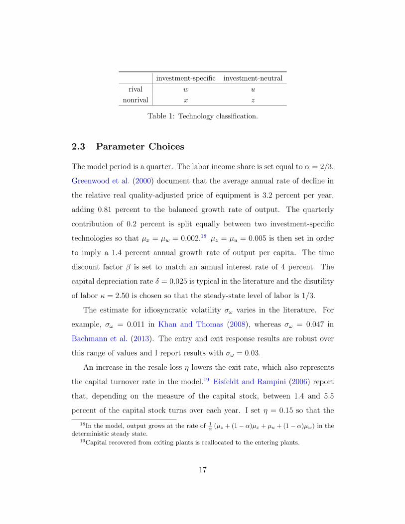
Table 1 summarizes four types of technology in the model.
The equilibrium conditions of the model (see Appendix A) are functional
equations that require solving for the distribution of plant productivity. To
deal with this infinite dimensional problem, I adopt an approach developed by
Campbell (1998) of approximating the distribution functions by their values at
a large but finite set of grid points and then applying a perturbation method
that can handle many state variables relatively easily. I obtain the solution by
using Dynare++ (Kamenik, 2011).
16
investment-specific investment-neutral
rival w u
nonrival x z
Table 1: Technology classification.
2.3 Parameter Choices
The model period is a quarter. The labor income share is set equal to α = 2/3.
Greenwood et al. (2000) document that the average annual rate of decline in
the relative real quality-adjusted price of equipment is 3.2 percent per year,
adding 0.81 percent to the balanced growth rate of output. The quarterly
contribution of 0.2 percent is split equally between two investment-specific
technologies so that µx = µw = 0.002.18 µz = µu = 0.005 is then set in order
to imply a 1.4 percent annual growth rate of output per capita. The time
discount factor β is set to match an annual interest rate of 4 percent. The
capital depreciation rate δ = 0.025 is typical in the literature and the disutility
of labor κ = 2.50 is chosen so that the steady-state level of labor is 1/3.
The estimate for idiosyncratic volatility σω varies in the literature. For
example, σω = 0.011 in Khan and Thomas (2008), whereas σω = 0.047 in
Bachmann et al. (2013). The entry and exit response results are robust over
this range of values and I report results with σω = 0.03.
An increase in the resale loss η lowers the exit rate, which also represents
the capital turnover rate in the model.19 Eisfeldt and Rampini (2006) report
that, depending on the measure of the capital stock, between 1.4 and 5.5
percent of the capital stock turns over each year. I set η = 0.15 so that the
18In the model, output grows at the rate of 1α (µz + (1− α)µx + µu + (1− α)µw) in the
deterministic steady state.19Capital recovered from exiting plants is reallocated to the entering plants.
17

annual turnover rate of capital is 3.2 percent in the steady state.20
Finally, the standard deviation of the entrant’s initial productivity distri-
bution is set to σe = 0.09, which is much larger than the idiosyncratic volatility
σω based on the finding that entering plants face a higher productivity uncer-
tainty than old plants (Bartelsman and Dhrymes, 1999). I experiment with a
wide range of values for this parameter as well as others and the qualitative
results remain intact.
2.4 Effects of Technology Shocks
Figure 1 displays the impulse responses of the entry and exit thresholds (ωt
and ωt), the entry and exit rates21, and the quality-adjusted price of capital
goods Pt to four technology shocks in the model.22 The stochastic trend of
output in the model is 1α
(zt + (1− α)xt + ut + (1− α)wt). Hence, I consider
a 1 percent shock to each technology—zt, (1− α)xt, ut, (1− α)wt—so that all
four shocks have the same size effect on output—a 1α
percent increase—in the
long run. The pool of new ideas H t is also set to jump upon impact to a new
steady state value.
All four technology shocks encourage entry. Although the new idea pool
increases by the same percentage, a rise in entry is bigger than an increase in
the steady state level during the transition; this results in a lower entry thresh-
old for nonrival technology shocks. The incumbent plants then compete with
new plants that have lower productivity, thereby reducing the exit threshold
and the exit rate. In contrast, rival technology shocks induce a rise in the
20More precisely, η and the (normalized) level of the new idea pool—H?
in AppendixA—are set to imply a capital turnover rate of 3.2 percent and an investment to output ratioof 20 percent in the steady state.
21
∫∞ωtHt(ωt)dωt∫∞
−∞Kt(ωt)dωtand
∫ ωt−∞Kt(ωt)dωt∫∞−∞Kt(ωt)dωt
.
22See Appendix C for the impulse responses of key macroeconomic variables.
18

10 20 30 40−8
−6
−4
−2
0x 10
−4
quarters
Entry threshold
10 20 30 40−6
−4
−2
0x 10
−4
quarters
Exit threshold
10 20 30 400
0.02
0.04
0.06
0.08
pe
rce
nt
quarters
Entry rate
10 20 30 40−0.02
−0.01
0
0.01
pe
rce
nt
quarters
Exit rate
10 20 30 40−1
−0.5
0
0.5
1
pe
rce
nt
quarters
Capital price
10 20 30 40−2
−1.5
−1
−0.5
0x 10
−3
quarters
Entry threshold
10 20 30 40−2
−1.5
−1
−0.5
0x 10
−3
quarters
Exit threshold
10 20 30 400
0.1
0.2
0.3
pe
rce
nt
quarters
Entry rate
10 20 30 40−0.06
−0.04
−0.02
0
0.02
pe
rce
nt
quarters
Exit rate
10 20 30 40−3
−2
−1
0
pe
rce
nt
quarters
Capital price
10 20 30 400
0.002
0.004
0.006
0.008
0.01
quarters
Entry threshold
10 20 30 400
0.002
0.004
0.006
0.008
0.01
quarters
Exit threshold
10 20 30 400
0.05
0.1
0.15
pe
rce
nt
quarters
Entry rate
10 20 30 400
0.05
0.1
0.15
0.2
pe
rce
nt
quarters
Exit rate
10 20 30 40−1
−0.5
0
0.5
1
pe
rce
nt
quarters
Capital price
10 20 30 40−4
−3
−2
−1
0x 10
−3
quarters
Entry threshold
10 20 30 400
0.002
0.004
0.006
0.008
0.01
quarters
Exit threshold
10 20 30 400
0.05
0.1
0.15
pe
rce
nt
quarters
Entry rate
10 20 30 400
0.05
0.1
0.15
0.2p
erc
en
t
quarters
Exit rate
10 20 30 40−3
−2
−1
0
pe
rce
nt
quarters
Capital price
Figure 1: Impulse responses of entry and exit to a 1 percent increase in nonrivalinvestment-neutral technology zt (top panel), nonrival investment-specific technol-ogy (1 − α)xt (second panel), rival investment-neutral technology ut (third panel),and rival investment-specific technology (1− α)wt (bottom panel).
productivity of new plants and the resulting competition with a better cohort
of entrants pushes out old plants. Note that although the entry threshold for
new ideas drops in the case of a rival investment-specific technology shock
(bottom panel), those ideas are equipped with a better quality capital so that
the productivity of new plants rise.23 Hence, the exit rate rises for both rival
23In fact, if we plot the entry threshold for an entrant’s productivity after her productivityis enhanced by more efficient capital (ωt in Appendix A), the response is exactly the sameas that of a rival investment-neutral technology shock. See footnote 15 and Appendix A.
19

technology shocks.
The different signs of the exit responses, of course, depend on how elas-
tically the pool of new ideas responds to the shocks; however, the different
sizes of the exit responses are more robust. Note that the response of the exit
rate is an order of magnitude smaller than that of the entry rate in the case
of nonrival technology shocks. This comes from the fact that these shocks
do not affect new and old plants differentially: a nonrival investment-neutral
technology shock makes both new and old capital more productive, while a
nonrival investment-specific technology shock lowers the value of new capital
as well as the scrap value of old capital. In contrast, rival technology shocks
increase both the entry and exit rates by a similar magnitude; only new units
become more productive and this widened productivity gap between entrants
and incumbents makes old plants more valuable in a sell-off as their capital
can be deployed by more productive entrants.24
I will later show that the empirical impulse responses to the investment-
specific technology shocks are characterized by a lead-lag pattern—the entry
and job creation rates rise on impact, whereas the exit and job destruction
rates initially fall but subsequently rise above the average for an extended
amount of time. This response is predicted by a version of the model, which
is extended to assume that more than one time period is required for an exit
and job destruction.25
24This result is similar to Michelacci and Lopez-Salido (2007), who show in a searchmodel that investment-neutral technological advances increase job destruction and realloca-tion; whereas, investment-specific technological advances that make new capital equipmentless expensive reduce job destruction. The authors assume old plants can adopt investment-neutral technology with a small probability; hence, this technology is closer to rival tech-nology than the nonrival investment-neutral technology studied in my model.
25The responses of the existing plants to a new wave of entrants are likely to take asubstantial time in the real world. Liquidating and selling off existing assets takes time. Inaddition to physical frictions, the delay can be due to informational frictions: the incumbents
20

3 Empirical Approach
3.1 Identification
Consider the vector moving average representation of a VAR:
yt = C(L)ut, (7)
where yt is a n×1 vector, C(L) = I+C1L+C2L2+. . . is a matrix of polynomials
in the lag operator L, and ut is a n × 1 vector of one-step ahead forecasting
errors with a variance-covariance matrix E[utu′t] = Σ. Identification of the
structural shocks amounts to finding a matrix A and a vector of mutually
orthogonal shocks εt, such that ut = Aεt.
The elements of yt are [∆pt,∆at,∆ht, enrt, exrt]′, where pt is the log of the
quality-adjusted capital good price, at is the log of labor productivity, ht is
the log of per capita hours worked,26 enrt is the entry rate, exrt is the exit
rate, and ∆ = 1− L.
This paper identifies the reallocation shock by extracting the shock that
explains the maximal amount of the FEV over the business cycle horizon up to
32 quarters for the turnover rate enrt + exrt.27 First, fix A to some arbitrary
might not immediately realize that the entrants have better productivity. See Appendix Dfor the impulse responses with a time-to-exit assumption.
26I consider the differenced hours as my benchmark case. The literature on the long-run identification of technology shocks reaches different conclusions depending on how re-searchers deal with the low frequency variation in hours (e.g., Gali, 1999, and Christianoet al., 2004). This literature typically finds that the technology shocks are less expansion-ary and account for a smaller fraction of hours variation when hours enters the VAR as indifferences rather than in levels. I indeed find stronger results with the level specification.
27This identification strategy to extract shocks that explain the majority of FEV of atarget variable is developed by Uhlig (2003) and is adopted in Barsky and Sims (2011),Kurmann and Otrok (2013), and Francis et al. (2014). Such identified shocks in generaldepend on the forecast horizon over which the FEV is maximized. The similarity between areallocation shock and an investment-specific technology shock remains strong in my study
21

matrix satisfying Σ = AA′. Finding A is then equivalent to choosing an
orthonomal matrix Q, such that ut = AQεt. The k-step ahead forecast error
of the turnover rate is given by:
enrt+k + exrt+k − Et(enrt+k + exrt+k) = e′i
[k−1∑l=0
ClAQεt+k−l
],
where ei is a column vector with 1 in the 4th and 5th positions and 0 elsewhere.
Let q be a column vector of Q. I then solve
q = arg maxq
e′i
k∑k=k
k−1∑l=0
ClAqq′AC ′l
ei subject to q′q = 1
so that q′A−1ut is a reallocation shock.
For comparison, I also identify the investment-specific technology shock fol-
lowing Fisher (2006). I impose all first-row elements except the (1, 1) position
of C(1)A to be equal to zero so that only the investment-specific technology
shock has a long-run impact on the capital good price. The investment-neutral
technology shock can in turn be identified by imposing that all second-row el-
ements except the (2, 1) and (2, 2) positions of C(1)A are equal to zero. Table
2 summarizes the long-run restrictions.
ShocksPermanent effects on:
capital price labor productivity
investment-specific technology shock yes yes
investment-neutral technology shock no yes
all other shocks no no
Table 2: Identification by long-run restrictions.
unless I focus on a short forecast horizon of less than three years.
22
3.2 Data
The real price of quality-adjusted capital goods is an investment deflator for
equipment and software divided by a consumption deflator for nondurables
and services. This series is constructed by Liu et al. (2011),28 who adopt the
method used by Fisher (2006)29 and extend the series to more recent periods.
Labor productivity is measured by the nonfarm business series published by
the Bureau of Labor Statistics (BLS).30 Following Fisher (2006), productivity
is also expressed in consumption units using the same consumption deflator
that underlies the capital goods price. Per capita hours are measured with
the BLS hours series for the nonfarm business sector divided by the civilian
noninstitutionalized population over the age of 16.
For the entry and exit rates, I use the rates of total private sector establish-
ment births and deaths from the BLS Business Employment Dynamics (BED)
data. The BED series are quarterly and seasonally adjusted and they have
been available since 1993:II. The BED defines births as those records that
have positive employment in the third month of a quarter and zero employ-
ment in the third month of the previous four quarters. Similarly, deaths are
units that report zero employment in the third month of a quarter and do not
report positive employment in the subsequent third months of the next four
quarters.
28Their benchmark series is the quality-adjusted deflator for equipment and software,nonresidential and residential structures, and consumer durables. I instead use a versionincluding equipment and software only because the technology embodied in equipment andsoftware better represents the type of technology I am interested in; that is, innovationthat requires restructuring the production unit. My results are slightly stronger with thisdeflator for equipment and software only, but the difference is small. Fisher (2006) also usesthe deflator for only equipment and software as his benchmark deflator.
29Fisher (2006) builds on Gordon (1990) and Cummins and Violante (2002).30Fernald (2012) constructs a quarterly utilization-adjusted series on TFP. I also use his
measure of TFP instead of labor productivity and find very similar results.
23

The BLS BED data contain job flow rates as well. Job creation and de-
struction rates are defined as private sector gross job gains and job losses,
respectively, as a percent of employment. This data have also been available
since 1993:II, and these series are quarterly and seasonally adjusted.
I also consider the capital turnover rates used by Eisfeldt and Rampini
(2006). They construct two capital turnover rates from the annual Com-
pustat data—acquisitions divided by lagged total assets as well as sales of
property, plant, and equipment divided by lagged total property, plant, and
equipment. To obtain more observations, I follow Cui (2013) to construct the
corresponding quarterly series from the quarterly Compustat data and apply
a X-12-ARIMA seasonal adjustment.
Appendix E provides a time-series plot and summary statistics of this data.
4 Empirical Findings
The sample period used in this paper is 1993:II–2014:II. The baseline VAR are
estimated with 4 lags of each variable and no time trend. To compute error
bands, I impose a diffuse (Jeffreys) prior and display 68 percent error bands.
4.1 Baseline Estimates
Figure 2 shows the impulse responses to reallocation shocks identified by maxi-
mizing the FEV. The investment price keeps falling and the labor productivity
gradually increases after an initial rise and drop. Hours respond positively and
with a hump shape; the entry rate immediately rises and gradually declines,
whereas the exit rate rises significantly above zero after two-and-a-half years.
Figure 3 displays the fraction of the FEV explained by the reallocation
24

5 10 15 20 25 30 35 40
−3.5
−3
−2.5
−2
−1.5
−1
−0.5
0
Investment price
pe
rce
nt
quarters5 10 15 20 25 30 35 40
0
0.5
1
1.5
2
2.5
Labor productivity
pe
rce
nt
quarters5 10 15 20 25 30 35 40
−3
−2.5
−2
−1.5
−1
−0.5
0
0.5
1
1.5
2
Hours
pe
rce
nt
quarters
5 10 15 20 25 30 35 40
0
0.01
0.02
0.03
0.04
0.05
0.06
0.07
0.08
0.09
Entry rate
pe
rce
nt
quarters5 10 15 20 25 30 35 40
−0.04
−0.02
0
0.02
0.04
0.06
Exit rate
pe
rce
nt
quarters5 10 15 20 25 30 35 40
0
0.02
0.04
0.06
0.08
0.1
0.12
Turnover rate
pe
rce
nt
quarters
Figure 2: Impulse responses to a reallocation shock based on entry and exit data.
0 10 20 30 400
0.1
0.2
0.3
0.4
0.5
0.6
0.7
0.8
0.9
1
Investment price
fra
ctio
n o
f F
EV
exp
lain
ed
quarters0 10 20 30 40
0
0.1
0.2
0.3
0.4
0.5
0.6
0.7
0.8
0.9
1
Labor productivity
fra
ctio
n o
f F
EV
exp
lain
ed
quarters0 10 20 30 40
0
0.1
0.2
0.3
0.4
0.5
0.6
0.7
0.8
0.9
1
Hours
fra
ctio
n o
f F
EV
exp
lain
ed
quarters
0 10 20 30 400
0.1
0.2
0.3
0.4
0.5
0.6
0.7
0.8
0.9
1
Entry rate
fra
ctio
n o
f F
EV
exp
lain
ed
quarters0 10 20 30 40
0
0.1
0.2
0.3
0.4
0.5
0.6
0.7
0.8
0.9
1
Exit rate
fra
ctio
n o
f F
EV
exp
lain
ed
quarters0 10 20 30 40
0
0.1
0.2
0.3
0.4
0.5
0.6
0.7
0.8
0.9
1
Turnover rate
fra
ctio
n o
f F
EV
exp
lain
ed
quarters
Figure 3: Fraction of forecast error variance (FEV) explained by reallocation shockbased on entry and exit data.
shock. It is noteworthy that the reallocation shock accounts for most medium-
25

and longer-term variations in the turnover rate. This shock by construction
maximizes its contribution among possible shocks, but nothing requires that
a single shock account for over 50 to 75 percent of all unpredictable fluctua-
tions from one-and-a-half to ten years. Hence, the identified shock is truly a
dominant driving force behind fluctuations in reallocation.
5 10 15 20 25 30 35 40
−3.5
−3
−2.5
−2
−1.5
−1
−0.5
0
Investment price
perc
ent
quarters5 10 15 20 25 30 35 40
0
0.5
1
1.5
2
Labor productivity
perc
ent
quarters5 10 15 20 25 30 35 40
−1.5
−1
−0.5
0
0.5
1
1.5
2
2.5
Hours
perc
ent
quarters
5 10 15 20 25 30 35 40
0
0.01
0.02
0.03
0.04
0.05
0.06
0.07
0.08
0.09
Entry rate
perc
ent
quarters5 10 15 20 25 30 35 40
−0.06
−0.04
−0.02
0
0.02
0.04
0.06
Exit rate
perc
ent
quarters5 10 15 20 25 30 35 40
−0.02
0
0.02
0.04
0.06
0.08
0.1
0.12
Turnover rate
perc
ent
quarters
Figure 4: Impulse responses to an investment-specific technology shock based onentry and exit data.
Figure 4 displays the impulse responses to investment-specific technology
shocks identified by the long-run restrictions. These results are very similar
to the results for reallocation shocks. The initial drop of the exit rate is more
significant, but as mentioned earlier, this pattern of a lagged response of exit
is consistent with a version of the model extended to include the time to
exit. The fraction of the FEV explained by the investment-specific technology
shock (Figure 5) is also very similar.31 The investment-specific technology
31As can be expected from the result that most variations in entry and turnover rates areaccounted for by investment-specific technology shocks, the responses of reallocation rates
26

0 10 20 30 400
0.1
0.2
0.3
0.4
0.5
0.6
0.7
0.8
0.9
1
Investment price
fra
ctio
n o
f F
EV
exp
lain
ed
quarters0 10 20 30 40
0
0.1
0.2
0.3
0.4
0.5
0.6
0.7
0.8
0.9
1
Labor productivity
fra
ctio
n o
f F
EV
exp
lain
ed
quarters0 10 20 30 40
0
0.1
0.2
0.3
0.4
0.5
0.6
0.7
0.8
0.9
1
Hours
fra
ctio
n o
f F
EV
exp
lain
ed
quarters
0 10 20 30 400
0.1
0.2
0.3
0.4
0.5
0.6
0.7
0.8
0.9
1
Entry rate
fra
ctio
n o
f F
EV
exp
lain
ed
quarters0 10 20 30 40
0
0.1
0.2
0.3
0.4
0.5
0.6
0.7
0.8
0.9
1
Exit rate
fra
ctio
n o
f F
EV
exp
lain
ed
quarters0 10 20 30 40
0
0.1
0.2
0.3
0.4
0.5
0.6
0.7
0.8
0.9
1
Turnover rate
fra
ctio
n o
f F
EV
exp
lain
ed
quarters
Figure 5: Fraction of forecast error variance (FEV) explained by investment-specifictechnology shock based on entry and exit data.
shock accounts for more than 35 percent of hours variation after one year,
confirming that it is a major shock driving the business cycle fluctuations.
Fisher (2006) finds that the investment-specific technology shock accounts for
9 to 22 percent of hours’ FEV in the sample period of 1982:III–2000:IV. Figure
5 shows that the importance of an investment-specific technology shock is even
larger in the more recent periods of 1993:II–2014:II, the time period studied
in this paper.
The identified investment-specific technology shocks are conceptually a
weighted average of rival and nonrival shocks (shocks to w and x in Section 2).
The strong positive effects on reallocation suggest that the identified shocks
to investment-neutral technology shocks (not shown) are weak and the error bands includezero in most periods. In addition, the hours response is no longer robust across differentspecifications: hours fall (rise) after a positive investment-neutral technology shock whenhours enters the VAR in differences (in levels with/without time trends). I find the sameresults for job flow and capital reallocation data as well.
27

5 10 15 20 25 30 35 40−1.8
−1.6
−1.4
−1.2
−1
−0.8
−0.6
−0.4
−0.2
0
Investment price pe
rcen
t
quarters5 10 15 20 25 30 35 40
−0.6
−0.4
−0.2
0
0.2
0.4
Labor productivity
perc
ent
quarters5 10 15 20 25 30 35 40
0
0.5
1
1.5
2
2.5
3
Hours
perc
ent
quarters
5 10 15 20 25 30 35 400
0.02
0.04
0.06
0.08
0.1
0.12
0.14
0.16
0.18
Job creation rate
perc
ent
quarters5 10 15 20 25 30 35 40
−0.1
−0.05
0
0.05
0.1
Job destruction rate
perc
ent
quarters5 10 15 20 25 30 35 40
0
0.05
0.1
0.15
0.2
Job reallocation rate
perc
ent
quarters
Figure 6: Impulse responses to an investment-specific technology shock based onjob flow data.
0 10 20 30 400
0.1
0.2
0.3
0.4
0.5
0.6
0.7
0.8
0.9
1
Investment price
fract
ion
of F
EV
exp
lain
ed
quarters0 10 20 30 40
0
0.1
0.2
0.3
0.4
0.5
0.6
0.7
0.8
0.9
1
Labor productivity
fract
ion
of F
EV
exp
lain
ed
quarters0 10 20 30 40
0
0.1
0.2
0.3
0.4
0.5
0.6
0.7
0.8
0.9
1
Hours
fract
ion
of F
EV
exp
lain
ed
quarters
0 10 20 30 400
0.1
0.2
0.3
0.4
0.5
0.6
0.7
0.8
0.9
1
Job creation rate
fract
ion
of F
EV
exp
lain
ed
quarters0 10 20 30 40
0
0.1
0.2
0.3
0.4
0.5
0.6
0.7
0.8
0.9
1
Job destruction rate
fract
ion
of F
EV
exp
lain
ed
quarters0 10 20 30 40
0
0.1
0.2
0.3
0.4
0.5
0.6
0.7
0.8
0.9
1
Job reallocation rate
fract
ion
of F
EV
exp
lain
ed
quarters
Figure 7: Fraction of forecast error variance (FEV) explained by investment-specifictechnology shock based on job flow data.
28

are mostly rival (shocks to w).32
I also find similar results for other reallocation measures. Figures 6 and 7
show the results when job creation and destruction rates are used in place of
entry and exit rates. As the results for the reallocation shock are very similar,
they are omitted from this paper. The investment-specific technology shock
explains over 50 percent of the job reallocation rate’s FEV for three to ten
years. The impulse responses are similar to that seen in the case of entry and
exit data and the only notable difference is that labor productivity falls below
zero in the medium term. Note, however, that output still rises as the hours
response is larger than the productivity response.
The positive responses of job creation and reallocation rates to an investment-
specific technology shock are different from the results of Michelacci and Lopez-
Salido (2007), who find that this shock leads to a fall in job destruction and
reallocation rates. This difference in findings results from different data sam-
ples being used in these two studies. Michelacci and Lopez-Salido (2007) use a
quarterly series of job flow data in the manufacturing sector for 1972:I–1993:IV;
I in fact find similar results to theirs when using this data (see Appendix F).
Interestingly, the contribution of the investment-specific technology shock
to the long-run variation in labor productivity differs substantially among the
two samples. The investment-specific technology shock accounts for less than
30 percent of the permanent change in labor productivity in the manufacturing
sector for 1972:I–1993:IV, whereas it accounts for about 80 percent in the total
private sector for 1993:II–2014:II (see Table 3). In other words, the technol-
ogy shocks identified by long-run restrictions in the former sample are mostly
32Similarly, the identified reallocation shocks are in principle a combination of multipleshocks; however, the close relationship between reallocation and investment-specific tech-nology shocks suggests that the identified reallocation shocks are mostly investment-specifictechnology shocks (shocks to w).
29

5 10 15 20 25 30 35 40
−3.5
−3
−2.5
−2
−1.5
−1
−0.5
0
Investment price pe
rcen
t
quarters5 10 15 20 25 30 35 40
0
0.5
1
1.5
2
Labor productivity
perc
ent
quarters5 10 15 20 25 30 35 40
−1
−0.5
0
0.5
1
1.5
2
Hours
perc
ent
quarters
5 10 15 20 25 30 35 40
−0.005
0
0.005
0.01
0.015
0.02
0.025
0.03
0.035
Acquisitions turnover rate
perc
ent
quarters5 10 15 20 25 30 35 40
0
0.01
0.02
0.03
0.04
0.05
Property sale turnover rate
perc
ent
quarters5 10 15 20 25 30 35 40
−0.01
0
0.01
0.02
0.03
0.04
0.05
0.06
0.07
0.08
Sum of turnover rates
perc
ent
quarters
Figure 8: Impulse responses to an investment-specific technology shock based oncapital reallocation data.
0 10 20 30 400
0.1
0.2
0.3
0.4
0.5
0.6
0.7
0.8
0.9
1
Investment price
fract
ion
of F
EV
exp
lain
ed
quarters0 10 20 30 40
0
0.1
0.2
0.3
0.4
0.5
0.6
0.7
0.8
0.9
1
Labor productivity
fract
ion
of F
EV
exp
lain
ed
quarters0 10 20 30 40
0
0.1
0.2
0.3
0.4
0.5
0.6
0.7
0.8
0.9
1
Hours
fract
ion
of F
EV
exp
lain
ed
quarters
0 10 20 30 400
0.1
0.2
0.3
0.4
0.5
0.6
0.7
0.8
0.9
1
Acquisitions turnover rate
fract
ion
of F
EV
exp
lain
ed
quarters0 10 20 30 40
0
0.1
0.2
0.3
0.4
0.5
0.6
0.7
0.8
0.9
1
Property sale turnover rate
fract
ion
of F
EV
exp
lain
ed
quarters0 10 20 30 40
0
0.1
0.2
0.3
0.4
0.5
0.6
0.7
0.8
0.9
1
Sum of turnover rates
fract
ion
of F
EV
exp
lain
ed
quarters
Figure 9: Fraction of forecast error variance (FEV) explained by investment-specifictechnology shock based on capital reallocation data.
30

investment-neutral, whereas they are mostly investment-specific in the latter
one. Hence, the dominant technology shocks enhance job reallocation in both
samples,33 which is in line with the positive relationship between reallocation
and productivity growth documented in the productivity literature.34
Figures 8 and 9 display the results when capital turnover rates are used.
The elements of yt in the VAR system (7) are [∆pt,∆at,∆ht, tr1t , tr
2t ]′, where
tr1t is acquisitions divided by lagged total assets and tr2
t is the sales of property,
plant, and equipment divided by lagged total property, plant, and equipment.35
Note that both turnover rates are reallocation measures,36 whereas only the
sum of the entry and exit rates—or the sum of the job creation and destruction
rates—represents reallocation in the previous cases. This explains why both
rates rise together without a lead-lag pattern. The fraction of the FEV ex-
plained by the investment-specific technology shock is again large—it explains
over 50 percent of the variations of the capital turnover rates after three years.
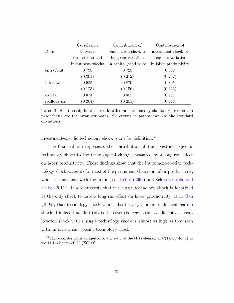
The tight link between reallocation and investment-specific technology
shocks can also be seen in Table 3. The mean estimates of the correlation
coefficient between the two shocks are over 0.79 for all three reallocation mea-
sures. The contribution of the reallocation shock to the long-run variation in
the capital goods price is also over 0.72. Note that the contribution of the
33However, the hours response differs. The investment-neutral technology shock in theearlier sample is contractionary, whereas the investment-specific technology shock in thelater sample is expansionary.
34The findings in this literature are mainly based on cross-sectional decomposition—thosestudies decompose the total industry-wide productivity growth over the sample period intocomponents that reflect an improvement in individual units and the reallocation of resourcesacross units. They find that the reallocation component is substantial. See Foster et al.(2001) and references therein.
35The correlation coefficient of these two series is 0.56.36A reallocation shock is again identified as a shock that explains the maximum amount
of the FEV of the sum of the two turnover rates tr1t + tr2t . The results are very similar andare therefore omitted.
31
Correlation Contribution of Contribution of
Data between reallocation shock to investment shock to
reallocation and long-run variation long-run variation
investment shocks in capital good price in labor productivity
entry/exit 0.795 0.725 0.802
(0.301) (0.272) (0.242)
job flow 0.925 0.870 0.805
(0.123) (0.156) (0.226)
capital 0.874 0.805 0.787
reallocation (0.204) (0.201) (0.216)
Table 3: Relationship between reallocation and technology shocks. Entries not inparentheses are the mean estimates; the entries in parentheses are the standarddeviations.
investment-specific technology shock is one by definition.37
The final column represents the contribution of the investment-specific
technology shock to the technological change measured by a long-run effect
on labor productivity. These findings show that the investment-specific tech-
nology shock accounts for most of the permanent change in labor productivity,
which is consistent with the findings of Fisher (2006) and Schmitt-Grohe and
Uribe (2011). It also suggests that if a single technology shock is identified
as the only shock to have a long-run effect on labor productivity, as in Gali
(1999), that technology shock would also be very similar to the reallocation
shock. I indeed find that this is the case; the correlation coefficient of a real-
location shock with a single technology shock is almost as high as that seen
with an investment-specific technology shock.
37This contribution is computed by the ratio of the (1,1) element of C(1)Aqq′AC(1) tothe (1,1) element of C(1)ΣC(1)′.
32

4.2 Robustness
This subsection considers a number of potential specification issues. First, the
baseline estimates focus on a 5-variable VAR system primarily because the
quarterly reallocation measures of the total private sector are only available
for a short sample period. However, adding two more variables considered
by Fisher (2006)—nominal interest rate38 and inflation—barely changes the
strong link between the shock driving the reallocation and the investment-
specific technology shock.
Second, the baseline specification has hours included in differences. There
is a disagreement in the literature about the treatment of the low frequency
component of hours (see, for example, Gali, 1999; Christiano et al., 2004;
Francis and Ramey, 2005). The literature also considers the level specification
of hours with linear/quadratic detrending; these specifications lead to different
conclusions about whether hours rise or fall after a positive technology shock
and how important the role of the technology shocks is in explaining hours and
output fluctuations. I find that hours rise after a positive investment-specific
technology shock and that this shock accounts for over 30 percent of hours FEV
after one year for all those specifications. Hence, the prominent contribution
of the investment-specific technology shocks to cyclical fluctuations is very
robust for the sample period in this paper.
More importantly, I examine the robustness of the strong correlation be-
tween the reallocation shock and the investment-specific technology shock. I
find the correlation remains strong except for the entry and exit data; how-
ever, even in this case, the impulse responses to the two shocks are broadly
38Because the zero lower bound becomes binding in the latter part of my sample, I alsouse the Wu-Xia shadow Federal Funds rate (Wu and Xia, 2014) instead of the three-monthTreasury bill rate; however, the results do not change.
33

1996 1998 2000 2002 2004 2006 2008 2010 2012 2014−4
−2
0
2
4
pe
rce
nt
first differenced hours
1996 1998 2000 2002 2004 2006 2008 2010 2012 2014−6
−4
−2
0
2
4
pe
rce
nt
linear time trend
1996 1998 2000 2002 2004 2006 2008 2010 2012 2014−6
−4
−2
0
2
4
pe
rce
nt
quadratic time trend
Figure 10: Comparison of the reallocation shock (solid line) and the investment-specific technology shock (dash-dot line) based on entry and exit data. Correlationcoefficients are 0.92 (0.30, top panel), 0.49 (0.34, middle panel), and 0.53 (0.39,bottom panel). Numbers in parentheses are the standard deviations.
similar. To illustrate the dependence on different specifications, Figures 10,
11, and 12 extract the time series of the reallocation and investment-specific
technology shocks for the mean (OLS) estimates of the VAR parameters and
plot them together.39 I do not show the results for the level specification of
39I find that technology shocks account for a larger fraction of hours variations when thelevel specifications of hours with time trends are considered. This is consistent with thefindings of the aforementioned papers. The contribution to reallocation variations, however,becomes smaller than the benchmark case of differenced hours, as can be seen in the lowercorrelation coefficient.
34

1996 1998 2000 2002 2004 2006 2008 2010 2012 2014−4
−2
0
2
4
perc
ent
first differenced hours
1996 1998 2000 2002 2004 2006 2008 2010 2012 2014−2
−1
0
1
2
3
perc
ent
linear time trend
1996 1998 2000 2002 2004 2006 2008 2010 2012 2014−4
−2
0
2
4
perc
ent
quadratic time trend
Figure 11: Comparison of the reallocation shock (solid line) and the investment-specific technology shock (dash-dot line) based on job flow data. Correlation coeffi-cients are 0.95 (0.12, top panel), 0.82 (0.34, middle panel), and 0.82 (0.28, bottompanel). Numbers in parentheses are the standard deviations.
hours without the time trend because the extracted shocks are almost identical
with a correlation coefficient over 0.95. Although the correlation coefficients
are substantially smaller for the linear/quadratic trending in the case of the
entry and exit data, the two identified shocks broadly move together even in
this case. For all other cases, the two shocks very closely mirror each other
and represent a similar innovation to the economy.
35

1996 1998 2000 2002 2004 2006 2008 2010 2012 2014−4
−2
0
2
4
perc
ent
first differenced hours
1996 1998 2000 2002 2004 2006 2008 2010 2012 2014−6
−4
−2
0
2
4
perc
ent
linear time trend
1996 1998 2000 2002 2004 2006 2008 2010 2012 2014−6
−4
−2
0
2
4
perc
ent
quadratic time trend
Figure 12: Comparison of the reallocation shock (solid line) and the investment-specific technology shock (dash-dot line) based on capital reallocation data. Cor-relation coefficients are 0.93 (0.20, top panel), 0.87 (0.20, middle panel), and 0.91(0.29, bottom panel). Numbers in parentheses are the standard deviations.
5 Concluding Remarks
This paper studies two related questions: what drives cyclical movements in
reallocation and is the technological change rival or nonrival? By showing the
close link between the main shock affecting reallocation and the investment-
specific technology shock, I address these questions jointly. The investment-
specific technology shock is the dominant driving force behind reallocation; it
is the main technological progress accounting for a large portion of aggregate
36
fluctuations and is rival and disruptive.
My findings are subject to some caveats. Because of the data availability,
this study covers a relatively short sample period, which includes only two
recessions. It is hard to judge at this time whether the difference between my
findings and previous studies are due to a structural change in the 1990s or
factors unique to the Great Recession.
In addition, my results rely on the premise that the long-run restriction
identifies the exogenous technology shocks. A simple demand-side story can-
not explain my results because increased demand would lead to a higher price
of capital goods. However, if a higher demand encourages innovation in the
capital goods producing sector, resulting in a lower quality-adjusted price of
capital (in a way similar to Comin and Gertler, 2006), what I identify as a
disruptive innovation could be the confounding effects of various economic
shocks. Investigating the robustness of my findings to an endogenous techno-
logical change would be important and interesting and I hope to pursue this
matter in future research.
References
Abraham, Katharine G. and Lawrence F. Katz. 1986. Cyclical Unemployment:
Sectoral Shifts or Aggregate Disturbances? Journal of Political Economy
94 (3):507–522.
Acemoglu, Daron. 2009. Introduction to Modern Economic Growth. Princeton
University Press.
Aghion, Philippe and Peter Howitt. 1992. A Model of Growth Through Cre-
ative Destruction. Econometrica 60 (2):323–351.
37
Bachmann, Ruediger, Ricardo J. Caballero, and Eduardo M.R.A. Engel. 2013.
Aggregate Implications of Lumpy Investment: New Evidence and a DSGE
Model. American Economic Journal: Macroeconomics 5 (4):29–67.
Baldwin, John R., Timothy Dunne, and John C. Haltiwanger. 1993. Plant
Turnover in Canada and the United States. In The Dynamics of Industrial
Competition, edited by John R. Baldwin. Cambridge University Press.
Balleer, Almut. 2012. New Evidence, Old Puzzles: Technology Shocks and
Labor Market Dynamics. Quantitative Economics 3:363–392.
Barro, Robert J. and Robert G. King. 1984. Time-Separable Preferences and
Intertemporal-Substitution Models of Business Cycles. Quarterly Journal
of Economics 99 (4):817–839.
Barsky, Robert B. and Eric R. Sims. 2011. News Shocks and Business Cycles.
Journal of Monetary Economics 58:273–289.
Bartelsman, Eric J. and Phoebus J. Dhrymes. 1999. Productivity Dynamics:
U.S. Manufacturing Plants, 1972-1986. Journal of Productivity Analysis
9:5–34.
Bigio, Saki. 2015. Endogenous Liquidity and the Business Cycle. American
Economic Review 105 (6):1883–1927.
Blanchard, Olivier J. and Peter Diamond. 1989. The Beveridge Curve. Brook-
ings Papers on Economic Activity 1989 (1):1–60.
Caballero, Ricardo J. and Mohamad L. Hammour. 1996. On the Timing and
Efficiency of Creative Destruction. Quarterly Journal of Economics 111:805–
852.
38

———. 2005. The Cost of Recessions Revisited: A Reverse-Liquidationist
View. Review of Economic Studies 72:313–341.
Campbell, Jeffrey R. 1998. Entry, Exit, Embodied Technology, and Business
Cycles. Review of Economic Dynamics 1 (2):371–408.
Canova, Fabio, David Lopez-Salido, and Claudio Michelacci. 2013. The Ins and
Outs of Unemployment: An Analysis Conditional on Technology Shocks.
Economic Journal 123 (June):515–539.
Cao, Melanie and Shouyong Shi. 2016. Endogenously Procyclical Liquidity,
Capital Reallocation, and q. Working Paper.
Christiano, Lawrence J., Martin Eichenbaum, and Robert Vigfusson. 2004.
The Response of Hours to a Technology Shock: Evidence Based on Direct
Measures of Technology. Journal of the European Economic Association
2 (2-3):381–395.
Cochrane, John H. 1994. Shocks. Carnegie-Rochester Conference Series on
Public Policy 41:295–364.
Comin, Diego and Mark Gertler. 2006. Medium-Term Business Cycles. Amer-
ican Economic Review 96 (3):523–551.
Cui, Wei. 2013. Delayed Capital Reallocation. Working Paper.
Cummins, Jason G. and Giovanni L. Violante. 2002. Investment-Specific Tech-
nical Change in the United States (1947-2000): Measurement and Macroe-
conomic Consequences. Review of Economic Dynamics 5 (2):243–284.
39

Davis, Steven J. and John C. Haltiwanger. 1992. Gross Job Creation, Gross
Job Destruction, and Employment Reallocation. Quarterly Journal of Eco-
nomics 107 (3):819–863.
———. 1999a. Gross Job Flows. In Handbook of Labor Economics, vol. 3,
edited by Orley Ashenfelter and David Card. Elsevier.
———. 1999b. On the Driving Forces behind Cyclical Movements in Employ-
ment and Job Reallocation. American Economic Review 89 (5):1234–1258.
Davis, Steven J., R. Jason Faberman, and John C. Haltiwanger. 2006. The
Flow Approach to Labor Markets: New Data Sources and Micro-Macro
Links. Journal of Economic Perspectives 20 (3):3–26.
Eisfeldt, Andrea L. 2004. Endogenous Liquidity in Asset Markets. Journal of
Finance 59 (1):1–30.
Eisfeldt, Andrea L. and Adriano A. Rampini. 2006. Capital Reallocation and
Liquidity. Journal of Monetary Economics 53 (3):369–399.
Fernald, John G. 2007. Trend Breaks, Long-Run Restrictions, and Con-
tractionary Technology Improvements. Journal of Monetary Economics
54:2467–2485.
———. 2012. A Quarterly, Utilization-Adjusted Series on Total Factor Pro-
ductivity. Federal Reserve Bank of San Francisco Working Paper 2012-19.
Fisher, Jonas D. M. 2006. The Dynamic Effects of Neutral and Investment-
Specific Technology Shocks. Journal of Political Economy 114 (3):413–451.
Foster, Lucia, John Haltiwanger, and C. J. Krizan. 2001. Aggregate Produc-
tivity Growth. In New Developments in Productivity Analysis, edited by
40

Charles R. Hulten, Edwin R. Dean, and Michael J. Harper. University of
Chicago Press.
Foster, Lucia, Cheryl Grim, and John Haltiwanger. 2014. Reallocation in the
Great Recession: Cleansing or Not? NBER Working Paper 20427.
Francis, Neville and Valerie A. Ramey. 2005. Is the Technology-Driven Real
Business Cycle Hypothesis Dead? Shocks and Aggregate Fluctuations Re-
visited. Journal of Monetary Economics 52:1379–1399.
Francis, Neville, Michael T. Owyang, Jennifer E. Roush, and Riccardo DiCe-
cio. 2014. A Flexible Finite-Horizon Alternative to Long-Run Restrictions
with an Application to Technology Shocks. Review of Economics and Statis-
tics 96 (4):638–647.
Gali, Jordi. 1999. Technology, Emloyment, and the Business Cycle: Do Tech-
nology Shocks Explain Aggregate Fluctuations? American Economic Re-
view 89 (1):249–271.
Gordon, Robert J. 1990. The Measurement of Durable Goods Prices. University
of Chicago Press.
Greenwood, Jeremy, Zvi Hercowitz, and Gregory W. Huffman. 1988. Invest-
ment, Capacity Utilization, and the Real Business Cycle. American Eco-
nomic Review 78 (3):402–417.
Greenwood, Jeremy, Zvi Hercowitz, and Per Krusell. 1997. Long-Run Impli-
cations of Investment-Specific Technological Change. American Economic
Review 87 (3):342–362.
———. 2000. The Role of Investment-Specific Technological Change in the
Business Cycle. European Economic Review 44 (1):91–115.
41

Hopenhayn, Hugo A. 1992. Entry, Exit, and Firm Dynamics in Long Run
Equilibrium. Econometrica 60 (5):1127–1150.
Jaimovich, Nir and Sergio Rebelo. 2009. Can News about the Future Drive
the Business Cycle? American Economic Review 99 (4):1097–1118.
Justiniano, Alejandro, Giorgio E. Primiceri, and Andrea Tambalotti. 2010.
Investment Shocks and Business Cycles. Journal of Monetary Economics
57 (2):132–145.
Kamenik, Ondra. 2011. DSGE Models with Dynare++. A Tutorial.
Khan, Aubhik and Julia K. Thomas. 2008. Idiosyncratic Shocks and the Role of
Nonconvexities in Plant and Aggregate Investment Dynamics. Econometrica
76 (2):395–436.
Kurlat, Pablo. 2013. Lemons Markets and the Transmission of Aggregate
Shocks. American Economic Review 103 (4):1463–1489.
Kurmann, Andre and Christopher Otrok. 2013. News Shocks and the Slope
of the Term Structure of Interest Rates. American Economic Review
103:6:2612–2632.
Lanteri, Andrea. 2014. The Market for Used Capital: Endogenous Irreversibil-
ity and Reallocation over the Business Cycle. Working Paper.
Lee, Yoonsoo and Toshihiko Mukoyama. 2007. Entry, Exit, and Plant-level
Dynamics Over the Business Cycle. Federal Reserve Bank of Cleveland
Working Paper 07-18.
Li, Shaojin and Toni M. Whited. 2015. Capital Reallocation and Adverse
Selection. Working Paper.
42

Lilien, David M. 1982. Sectoral Shifts and Cyclical Unemployment. Journal
of Political Economy 90 (4):777–793.
Liu, Zheng, Daniel F. Waggoner, and Tao Zha. 2011. Sources of Macroeco-
nomic Fluctuations: A Regime-Switching DSGE Approach. Quantitative
Economics 2:251–301.
Michelacci, Claudio and David Lopez-Salido. 2007. Technology Shocks and
Job Flows. Review of Economic Studies 74 (4):1195–1227.
Ravn, Morten O. and Saverio Simonelli. 2007. Labor Market Dynamics and
the Business Cycle: Structural Evidence for the United States. Scandinavian
Journal of Economics 109 (4):743–777.
Samaniego, Roberto M. 2009. Entry, Exit, and Investment-Specific Technical
Change. American Economic Review 100 (1):164–192.
Schmitt-Grohe, Stephanie and Martin Uribe. 2011. Business Cycles with a
Common Trend in Neutral and Investment-specific Productivity. Review of
Economic Dynamics 14:122–135.
———. 2012. What’s News in Business Cycles. Econometrica 80 (6):2733–
2764.
Uhlig, Harald. 2003. What Drives GNP? Unpublished.
Wu, Jing Cynthia and Fan Dora Xia. 2014. Measuring the Macroeconomic
Impact of Monetary Policy at the Zero Lower Bound. NBER Working Paper
20117.
43

Appendix A First-order Conditions of the So-
cial Planner’s Problem
The social planner’s problem in Section 2.2 can be transformed in the following
ways. First, note that the labor allocation decision is atemporal so it can be
solved separately:
maxnt(·)
Yt =
∫ ∞−∞
ezt+ωtnt(ωt)αKt(ωt)dωt
subject to
Nt =
∫ ∞−∞
nt(ωt)Kt(ωt)dωt. (8)
The solution is
nt(ωt) =e
11−αωt
Kt
Nt, (9)
Yt =
∫ ∞−∞
ezt+ωtnt(ωt)αKt(ωt)dωt = eztK1−α
t Nαt , (10)
where
Kt =
∫ ∞−∞
e1
1−αωtKt(ωt)dωt (11)
is the productivity-weighted capital stock. Second, by replacing Ht(ωt) with
1σeφ(ωt−utσe
)×H t and applying a change of variable ωt = ωt + (1−α)wt, dωt =
dωt, the resulting integrals in equations (3) and (5) become
∫ ∞ωt
1
σeφ
(ωt − utσe
)H tdωt
=
∫ ∞ωt+(1−α)wt
1
σeφ
(ωt − ut − (1− α)wt
σe
)H tdωt,∫ ∞
ωt
1
σωφ
(ωt+1 − ωt − (1− α)wt
σω
)1
σeφ
(ωt − utσe
)H tdωt
44

=
∫ ∞ωt+(1−α)wt
1
σωφ
(ωt+1 − ωt
σω
)1
σeφ
(ωt − ut − (1− α)wt
σe
)H tdωt.
Once we define
ωt = ωt + (1− α)wt,
the social planner’s problem can be rewritten as:40
V (Kt(·), H t, zt, xt, ut, wt) = maxCt,Nt,ωt′ ,ωt′
(1− β) [logCt − κNt]
+βEt[V (Kt+1(·), H t+1, zt+1, xt+1, ut+1, wt+1)
],
subject to
eztK1−αt Nα
t = Ct + e−xt
[∫ ∞ωt
1
σeφ
(ωt − ut − (1− α)wt
σe
)H tdωt (12)
−(1− η)
∫ ωt
−∞Kt(ωt)dωt
],
Kt =
∫ ∞−∞
e1
1−αωtKt(ωt)dωt,
Kt+1(ωt+1) = (1− δ)∫ ∞ωt
1
σωφ
(ωt+1 − ωt
σω
)Kt(ωt)dωt (13)
+
∫ ∞ωt
1
σωφ
(ωt+1 − ωt
σω
)1
σeφ
(ωt − ut − (1− α)wt
σe
)H tdωt.
Note that this social planner’s problem is identical to one in which the capital
efficiency is not time varying and the initial productivity of potential entrants
is drawn from
ωt ∼ N(ut + (1− α)wt, σ2e)
40ωt is a dummy variable that is integrated out; hence, we can use ωt again—or anyletter—to denote this variable.
45

instead of (2).41 Hence two rival technologies, ut and wt, are isomorphic except
that their effects on the quality-adjusted price of capital goods P and the
original entry threshold ωt are different.42
The economy grows because of technological progress. To solve the social
planner’s problem, the problem must be transformed into a stationary one.
Expressing idiosyncratic productivity as a deviation from rival technologies,43
ω?t = ωt − ut−1 − (1− α)wt−1,
and dividing all variables except labor and entry/exit thresholds by the corre-
sponding stochastic trends,
C?t =
Ct
e1α
(zt+(1−α)xt+ut+(1−α)wt), K?
t (ω?t ) =Kt (ω?t + ut−1 + (1− α)wt−1)
e1α
(zt+xt+ut+(1−α)wt), . . . ,
accomplish this transformation. The resulting stationary problem is:
V ?(K?t (·),∆ut + (1− α)∆wt) = max
C?t ,Nt,ω?t ,ω
?t
(1− β) [logC?t − κNt] (14)
+βEt[V ?(K?
t+1(·),∆ut+1 + (1− α)∆wt+1)],
41Because the idea of the potential entrant who decides against entry disappears, allsurviving ideas in a given period are ones that are combined with capital in the sameperiod. Hence, it does not affect the outcome regardless of whether the initial productivityis shifted—ωt becomes ωt + (1− α)wt—before or after entry.
42ωt is the entry threshold for an entrant’s productivity before her initial productivity isshifted by (1− α)wt, whereas ωt is one after the productivity shift.
43Normalizing with respect to the lagged values of rival technologies is convenient be-cause the evolution of the normalized idiosyncratic productivity, ω?t to ω?t+1, is expressedas depending on the aggregate information up to the present, ∆ut + (1−α)∆wt, instead of∆ut+1 + (1− α)∆wt+1.
46

subject to
(K?t )1−αNα
t = C?t +
∫ ∞ω?t
1
σeφ
(ω?t −∆ut − (1− α)∆wt
σe
)H?dω?t
−(1− η)
∫ ω?t
−∞K?t (ω?t )dω
?t ,
K?t =
∫ ∞−∞
e1
1−α (ω?t−∆ut−(1−α)∆wt)K?t (ω?t )dω
?t ,
e1α
(∆zt+1+∆xt+1+∆ut+1+(1−α)∆wt+1)K?t+1(ω?t+1)
= (1− δ)∫ ∞ω?t
1
σωφ
(ω?t+1 − ω?t + ∆ut + (1− α)∆wt
σω
)K?t (ω?t )dω
?t
+
∫ ∞ω?t
1
σωφ
(ω?t+1 − ω?t + ∆ut + (1− α)∆wt
σω
)× 1
σeφ
(ω?t −∆ut − (1− α)∆wt
σe
)H?dω?t ,
where H?
is a constant number.
The Lagrangian for the problem is:
L = max (1− β) [logC?t − κNt] + βEt
[V ?(K?t+1(·),∆ut+1 + (1− α)∆wt+1
)]+Mt
[(K?
t )1−αNαt − Ct −
∫ ∞ω?t
1
σeφ
(ω?t −∆ut − (1− α)∆wt
σe
)H?dω?t
+(1− η)
∫ ω?t
−∞K?t (ω?t )dω
?t
]+MtDt
[∫ ∞−∞
e1
1−α (ω?t−∆ut−(1−α)∆wt)K?t (ω?t )dω
?t − K?
t
]
+Mt
∫ ∞−∞Qt(ω?t+1)
[(1− δ)
∫ ∞ω?t
1
σωφ
(ω?t+1 − ω?t + ∆ut + (1− α)∆wt
σω
)×K?
t (ω?t )dω?t +
∫ ∞ω?t
1
σωφ
(ω?t+1 − ω?t + ∆ut + (1− α)∆wt
σω
)× 1
σeφ
(ω?t −∆ut − (1− α)∆wt
σe
)H?dω?t
−e1α
(∆zt+1+∆xt+1+∆ut+1+(1−α)∆wt+1)K?t+1(ω?t+1)
]dω?t+1.
47

Note that the Lagrange multipliers44 Qt(ω?t+1) represent the value of a unit
of e1α
(∆zt+1+∆xt+1+∆ut+1+(1−α)∆wt+1)K?t+1(ω?t+1) =
Kt+1(ω?t+1+ut+(1−α)wt)
e1α (zt+xt+ut+(1−α)wt)
denomi-
nated in units of the normalized output Y ?t = Yt
e1α (zt+(1−α)xt+ut+(1−α)wt)
; equiva-
lently, Qt(ω?t+1) is the value of a unit of Kt+1(ωt+1) denominated in units of
(unnormalized) capital goods.
The first-order conditions are as follows:
• Optimal labor:
κ =1
C?t
× α
(K?t
Nt
)1−α
. (15)
The marginal disutility of labor equals the product of the marginal utility
of consumption and the marginal product of labor.
• Plant asset pricing45:
Qt(ω?t+1) = Et
[βe−
1α
(∆zt+1+∆xt+1+∆ut+1+(1−α)∆wt+1)
(C?t+1
C?t
)−1
(16)
×(
(1− α)
(K?t+1
Nt+1
)−αe
11−α(ω?t+1−∆ut+1−(1−α)∆wt+1)
+I(ω?t+1 ≤ ω?t+1)(1− η) + I(ω?t+1 > ω?t+1)(1− δ)
×∫ ∞−∞
1
σωφ
(ω?t+2 − ω?t+1 + ∆ut+1 + (1− α)∆wt+1
σω
)×Qt+1(ω?t+2)dω?t+2
)].
The value of a plant with the idiosyncratic productivity ω?t+1 is the ex-
44The other Lagrange multipliers are straightforward(Mt = 1−β
C?t, Dt = (1 −
α)
(K?t+1
Nt+1
)−α )and are substituted out in the following first-order conditions.
45I(·) is an indicator function.
48

pected discounted value of the following terms: the marginal product of
the plant with ω?t+1, the resale value of capital if the plant exits, and
the transition probability from ω?t+1 to ω?t+2 multiplied by the value of a
plant with ω?t+2 if the plant does not exit.
• Optimal entry:
1 =
∫ ∞−∞
1
σωφ
(ω?t+1 − ω?t + ∆ut + (1− α)∆wt
σω
)(17)
×Qt(ω?t+1)dω?t+1.
The marginal benefit of increasing the entry threshold ω?t is saving the
purchase cost of capital. The marginal cost is giving up the value of new
plant.
• Optimal exit:
1− η = (1− δ)∫ ∞−∞
1
σωφ
(ω?t+1 − ω?t + ∆ut + (1− α)∆wt
σω
)(18)
×Qt(ω?t+1)dω?t+1.
The marginal benefit of increasing the exit threshold ω?t is earning the
resale value of capital. The marginal cost is losing the continuation value
of the plant.
49

Appendix B Competitive Equilibrium and the
Social Planner’s Problem
B.1 Recursive Competitive Equilibrium
The aggregate state of the economy is described by Λt = (Kt(·), H t, zt, xt, ut, wt).
Denote the perceived law of motion for Kt(·) by Γk:
Kt+1(·) = Γk(Λt).
Let Mt,t+1 represent the stochastic discount factor between t and t + 146 and
W (Λt) represent the equilibrium wage rate.
To be well defined, the following problems must be transformed into sta-
tionary ones by appropriately scaling in a similar way to Appendix A. To avoid
an explosion of notation, the problems are stated below without scaling as if
all variables are stationary. A recursive competitive equilibrium is defined by
the following conditions:
• Plants optimally decide how much labor to hire and whether to exit the
market. The plant’s problem is:
46Mt,t+1(Λt,Λt+1) depends on the aggregate state of the economy in the current andnext periods. Its arguments are dropped for notational simplicity.
50

vk(ωt; Λt) = maxn
[ezt+ωtnα −W (Λt)n+ max
{(1− η)e−xt ,
(1− δ)∫ ∞−∞
1
σωφ
(ωt+1 − ωt
σω
)E[Mt,t+1v
k(ωt+1; Λt+1)∣∣∣Λt
]dωt+1
}]
= maxn,ω
[ezt+ωtnα −W (Λt)n+ I(ωt ≤ ω)(1− η)e−xt
+I(ωt > ω)(1− δ)∫ ∞−∞
1
σωφ
(ωt+1 − ωt
σω
)×E
[Mt,t+1v
k(ωt+1; Λt+1)∣∣∣Λt
]dωt+1
].
The policy functions are employment nk(ωt; Λt) and exit threshold ω(Λt),
which satisfy
nk(ωt; Λt) =α
11−α e
11−α (zt+ωt)
W (Λt)1
1−α(19)
(1− η)e−xt = (1− δ)∫ ∞−∞
1
σωφ
(ωt+1 − ω(Λt)
σω
)(20)
×E[Mt,t+1v
k(ωt+1; Λt+1)∣∣∣Λt
]dωt+1.
The resulting value (share price) of the plant is
vk(ωt; Λt) = (1− α)α
α1−α e
11−α (zt+ωt)
W (Λt)α
1−α(21)
+I(ωt ≤ ω(Λt))(1− η)e−xt + I(ωt > ω(Λt))(1− δ)
×∫ ∞−∞
1
σωφ
(ωt+1 − ωt
σω
)E[Mt,t+1v
k(ωt+1; Λt+1)∣∣∣Λt
]dωt+1.
• There are a mass H t of idea owners, who make the following once-and-
51

for-all decision about entry:
vh(ωt; Λt) = max
{0,−e−xt +
∫ ∞−∞
1
σωφ
(ωt+1 − ωt − (1− α)wt
σω
)×E
[Mt,t+1v
k(ωt+1; Λt+1)∣∣∣Λt
]dωt+1
},
where ωt is the idea owner’s productivity before it is shifted by (1−α)wt,
distributed by N(ut, σ2e). Equivalently, we can define the idea owner’s
problem in terms of the productivity after it is shifted by (1− α)wt:47
vh(ωt; Λt) = max
{0,−e−xt +
∫ ∞−∞
1
σωφ
(ωt+1 − ωt
σω
)×E
[Mt,t+1v
k(ωt+1; Λt+1)∣∣∣Λt
]dωt+1
},
where ωt is now distributed by N(ut + (1− α)wt, σ2e).
The policy function is the entry threshold ω(Λt), which satisfies
e−xt =
∫ ∞−∞
1
σωφ
(ωt+1 − ω(Λt)
σω
)(22)
×E[Mt,t+1v
k(ωt+1; Λt+1)∣∣∣Λt
]dωt+1.
The resulting value of the idea is
vh(ωt; Λt) = I(ωt > ω(Λt))
[− e−xt (23)
+
∫ ∞−∞
1
σωφ
(ωt+1 − ωt
σω
)E[Mt,t+1v
k(ωt+1; Λt+1)∣∣∣Λt
]dωt+1
].
47vh(ωt; Λt) = vh(ωt − (1− α)wt; Λt) holds. Also see footnote 41.
52

• Households’ state variables include their share holding of plants Kt(·) in
addition to aggregate state variables Λt. Note that households receive
endowments of ideas H t in each period. They solve:
vc(Kt(·),Λt) = maxc,nc,Kc(·)
(1− β) [log c− κnc] + βE[vc(Kc(·),Λt+1)|Λt],
subject to
c+
∫ ∞−∞
qk(ωt+1; Λt)Kc(ωt+1)dωt+1 = W (Λt)n
c (24)
+
∫ ∞−∞
vk(ωt; Λt)Kt(ωt)dωt
+
∫ ∞−∞
vh(ωt; Λt)1
σeφ
(ωt − ut − (1− α)wt
σe
)H tdωt,
where qk(ωt+1; Λt) is the current period share price of plants that begin
the next period with productivity ωt+1; that is,
qk(ωt+1; Λt) = E[Mt,t+1v
k(ωt+1,Λt+1)|Λt
]. (25)
The policy functions are consumption c(Kt(·),Λt), labor supply nc(Kt(·),Λt),
and shares of plants Kc(ωt+1; Kt(·),Λt), which satisfy
κ =1
c(Kt(·),Λt)W (Λt), (26)
qk(ωt+1; Λt) = E
β(c(Kt+1(·),Λt+1)
c(Kt(·),Λt)
)−1
vk(ωt+1; Λt+1)
∣∣∣∣∣Λt
(27)
• The labor market clears:
nc(Kt(·),Λt) =
∫ ∞−∞
nk(ωt; Λt)Kt(ωt)dωt. (28)
53

• The good market clears:
c(Kt(·),Λt) =
∫ ∞−∞
ezt+ωtnk(ωt; Λt)αKt(ωt)dωt (29)
−e−xt[∫ ∞
ω(Λt)
1
σeφ
(ωt − ut − (1− α)wt
σe
)H tdωt
−(1− η)
∫ ω(Λt)
−∞Kt(ωt)dωt
].
• The asset market clears:
Kc(ωt+1;Kt(·),Λt) = Kt+1(ωt+1) for all ωt+1. (30)
• Rational expectations: the economy indeed evolves as Kt+1(·) = Γk(Λt);
that is, for all ωt+1,
Γk(Λt)(ωt+1) = (1− δ)∫ ∞ω(Λt)
1
σωφ
(ωt+1 − ωt
σω
)Kt(ωt)dωt (31)
+
∫ ∞ω(Λt)
1
σωφ
(ωt+1 − ωt
σω
)1
σeφ
(ωt − ut − (1− α)wt
σe
)H tdωt.
Note that in equilibrium, households’ asset holding is equal to the economy-
wide capital stock:
Kt(·) = Kt(·), (32)
which is imposed in market clearing conditions (28)–(30).
B.2 Comparison
This subsection shows that the solution to the social planner’s problem in
Appendix A satisfies the conditions of recursive competitive equilibrium. Sup-
54

pose that C?t , Nt, ω
?t , ω
?t ,Qt(·) solves the problem (14) and the endogenous
state variable K?t (·) evolves accordingly. Consider the following allocations
and prices from the social planner’s problem:
nk(ωt; Λt) = nt(ω) (33)
ω(Λt) = ω?t + ut−1 + (1− α)wt−1 = ωt (34)
ω(Λt) = ω?t + ut−1 + (1− α)wt−1 = ωt (35)
c(Kt(·),Λt) = C?t e
1α
(zt+(1−α)xt+ut+(1−α)wt) = Ct (36)
nc(Kt(·),Λt) = Nt (37)
Kc(ωt+1;Kt(·),Λt) = K?t+1(ω?t+1)e
1α
(zt+1+xt+1+ut+1+(1−α)wt+1) (38)
= Kt+1(ωt+1)
Mt,t+1 = βe−1α
(∆zt+1+(1−α)∆xt+1+∆ut+1+(1−α)∆wt+1)
(C?t+1
C?t
)−1
(39)
= β
(Ct+1
Ct
)−1
W (Λt) = α
(K?t
Nt
)1−α
e1α
(zt+(1−α)xt+ut+(1−α)wt) (40)
= αezt
(Kt
Nt
)1−α
.
Because the competitive equilibrium conditions are presented with unscaled
variables, it is important to keep the correspondence between scaled and un-
scaled variables. The second, if any, equality in each of the above equations
are in terms of unscaled variables of the original—before being transformed
into a stationary one—social planer’s problem.48
48The second equality in equation (40) comes from
Kt =
∫ ∞−∞
e1
1−αωtKt(ωt)dωt
55

Substituting (34) and (40) into (21), we get:
vk(ωt; Λt) = (1− α)
(K?t
Nt
)−αe
11−α (ω?t−∆ut−(1−α)∆wt)e−xt
+I(ω?t ≤ ω?t )(1− η)e−xt + I(ω?t > ω?t )(1− δ)
×∫ ∞−∞
1
σωφ
(ω?t+1 − ω?t + ∆ut + (1− α)∆wt
σω
)×E
[Mt,t+1v
k(ωt+1; Λt+1)∣∣∣Λt
]dω?t+1.
Therefore, equation (25) implies
qk(ωt+1; Λt) = E[Mt,t+1v
k(ωt+1,Λt+1)|Λt
]= E
[Mt,t+1
((1− α)
(K?t+1
Nt+1
)−αe
11−α(ω?t+1−∆ut+1−(1−α)∆wt+1)e−xt+1
+I(ω?t+1 ≤ ω?t+1)(1− η)e−xt+1 + I(ω?t+1 > ω?t+1)(1− δ)
×∫ ∞−∞
1
σωφ
(ω?t+2 − ω?t+1 + ∆ut+1 + (1− α)∆wt+1
σω
)×qk(ωt+2; Λt+1)dω?t+2
)∣∣∣∣∣Λt
].
By comparing the above with equation (16) using (39), we obtain
qk(ωt+1,Λt) = Qt(ω?t+1)e−xt . (41)
In other words, the values of plants—vk(ωt; Λt), qk(ωt+1; Λt)—that are implied
by the allocations and prices considered in (33)–(40) satisfy equation (41).
Now examine whether these allocations and prices satisfy the conditions of
=
∫ ∞−∞
e1
1−α (ω?t+ut−1+(1−α)wt−1)K?t (ω?t )e
1α (zt+xt+ut+(1−α)wt)dω?t
= K?t e
1α (zt+xt+ 1
1−αut+wt).
56

recursive competitive equilibrium:
• Condition (19) is implied by equations (9), (33), and (40).
• Condition (20) is implied by equations (18), (25), (34), and (41).
• Condition (22) is implied by equations (17), (25), (35), and (41).
• Condition (24) is implied by equations (12) and (13): plugging equations
(21), (23), (25), (32), (34)–(38), and (40) into (24) gives
Ct +
∫ ∞−∞
qk(ωt+1; Λt)Kt+1(ωt+1)dωt+1
= αeztK1−αt Nα
t
+
∫ ∞−∞
[(1− α)ezt
(Kt
Nt
)−αe
11−αωt + I(ωt ≤ ωt)(1− η)e−xt
+I(ωt > ωt)(1− δ)∫ ∞−∞
1
σωφ
(ωt+1 − ωt
σω
)qk(ωt+1; Λt)dωt+1
]Kt(ωt)dωt
+
∫ ∞−∞
I(ωt > ωt)
[− e−xt +
∫ ∞−∞
1
σωφ
(ωt+1 − ωt
σω
)×qk(ωt+1; Λt)dωt+1
]1
σeφ
(ωt − ut − (1− α)wt
σe
)H tdωt
= αeztK1−αt Nα
t + (1− α)ezt
(Kt
Nt
)−α ∫ ∞−∞
e1
1−αωtKt(ωt)dωt
+(1− η)e−xt∫ ωt
−∞Kt(ωt)dωt
+
∫ ∞−∞
qk(ωt+1; Λt)
[(1− δ)
∫ ∞ωt
1
σωφ
(ωt+1 − ωt
σω
)Kt(ωt)dωt
]dωt+1
−e−xt∫ ∞ωt
1
σeφ
(ωt − ut − (1− α)wt
σe
)H tdωt +
∫ ∞−∞
qk(ωt+1; Λt)
×
[∫ ∞ωt
1
σωφ
(ωt+1 − ωt
σω
)1
σeφ
(ωt − ut − (1− α)wt
σe
)H tdωt
]dωt+1
= eztK1−αt Nα
t − e−xt[∫ ∞
ωt
1
σeφ
(ωt − ut − (1− α)wt
σe
)H tdωt
57

−(1− η)
∫ ωt
−∞Kt(ωt)dωt
]
+
∫ ∞−∞
qk(ωt+1; Λt)
[(1− δ)
∫ ∞ωt
1
σωφ
(ωt+1 − ωt
σω
)Kt(ωt)dωt
+
∫ ∞ωt
1
σωφ
(ωt+1 − ωt
σω
)1
σeφ
(ωt − ut − (1− α)wt
σe
)H tdωt
]dωt+1
where equation (11) is applied in the last equality; hence equation (24)
becomes
eztK1−αt Nα
t = Ct + e−xt
[∫ ∞ωt
1
σeφ
(ωt − ut − (1− α)wt
σe
)H tdωt
−(1− η)
∫ ωt
−∞Kt(ωt)dωt
]
+
∫ ∞−∞
qk(ωt+1; Λt)
[Kt(ωt+1)− (1− δ)
∫ ∞ωt
1
σωφ
(ωt+1 − ωt
σω
)Kt(ωt)dωt
−∫ ∞ωt
1
σωφ
(ωt+1 − ωt
σω
)1
σeφ
(ωt − ut − (1− α)wt
σe
)H tdωt
]dωt+1,
which is implied by equations (12) and (13).
• Condition (26) is implied by equations (15), (32), (36), and (40).
• Condition (27) is implied by equations (25), (32), (36), and (39).
• Condition (28) is implied by equations (8), (33), and (37).
• Condition (29) is implied by equations (10), (12), (34), (35), and (36).
• Condition (30) is implied by equation (38).
• Condition (31)—rational expectations—is trivially satisfied because all
agents’ perceived law of motion for Kt(·) is assumed to be the actual law
of motion for Kt(·) from the social planner’s problem.
58

Therefore, all conditions of recursive competitive equilibrium are satisfied
and the solution to the social planner’s problem indeed forms a competitive
equilibrium.
Appendix C Model Implications on Macroe-
conomic Variables
Figure 13 plots the impulse responses of key macroeconomic variables49 in the
model. Note that the responses in the last two panels are identical because
two rival technologies, ut and wt, are isomorphic except for their effects on the
quality-adjusted price of capital and the entry threshold (see Appendix A).
All four shocks lead to an economic expansion, but the initial responses to
shocks other than the first one do not exhibit a typical pattern of comovements.
First, consumption and labor move in opposite directions (bottom three
panels). This negative comovement of consumption and labor on the im-
pact of non-TFP shocks is common in the standard neoclassical growth model
(Barro and King, 1984): consumption and leisure are both normal goods and
therefore, unless shocks affect the relative price (marginal product of labor),
consumption and leisure move in the same direction.
Second, output and labor fall at the outset of the rival technology shocks
(bottom two panels). Innovation to the rival technologies in the model gradu-
ally spreads across the whole economy as a new generation of plants takes over
and thus it represents an anticipated increase in future TFP. The initial fall
of output and labor in response to a news shock is also common in neoclassi-
49Investment here is net investment, representing e−xt[∫∞ωtHt(ωt)dωt − (1− η)
∫ ωt−∞Kt(ωt)dωt
]in equation (3).
59

10 20 30 400
0.5
1
1.5
pe
rce
nt
quarters
Output
10 20 30 400
0.5
1
1.5
pe
rce
nt
quarters
Consumption
10 20 30 400
1
2
3
pe
rce
nt
quarters
Investment
10 20 30 400
0.1
0.2
0.3
0.4
pe
rce
nt
quarters
Labor
10 20 30 400
0.5
1
1.5
pe
rce
nt
quarters
Labor Productivity
10 20 30 400
0.5
1
1.5
pe
rce
nt
quarters
Output
10 20 30 40−0.5
0
0.5
1
1.5
pe
rce
nt
quarters
Consumption
10 20 30 400
2
4
6
8
10
pe
rce
nt
quarters
Investment
10 20 30 400
0.5
1
1.5
pe
rce
nt
quarters
Labor
10 20 30 40−0.5
0
0.5
1
1.5
pe
rce
nt
quarters
Labor Productivity
10 20 30 40−0.5
0
0.5
1
1.5
pe
rce
nt
quarters
Output
10 20 30 400
0.5
1
1.5
pe
rce
nt
quarters
Consumption
10 20 30 40−1
0
1
2
3
pe
rce
nt
quarters
Investment
10 20 30 40−0.2
0
0.2
0.4
pe
rce
nt
quarters
Labor
10 20 30 400
0.5
1
1.5
pe
rce
nt
quarters
Labor Productivity
10 20 30 40−0.5
0
0.5
1
1.5
pe
rce
nt
quarters
Output
10 20 30 400
0.5
1
1.5
pe
rce
nt
quarters
Consumption
10 20 30 40−1
0
1
2
3
pe
rce
nt
quarters
Investment
10 20 30 40−0.2
0
0.2
0.4p
erc
en
t
quarters
Labor
10 20 30 400
0.5
1
1.5
pe
rce
nt
quarters
Labor Productivity
Figure 13: Impulse responses of entry and exit to a 1 percent increase in nonrivalinvestment-neutral technology zt (top panel), nonrival investment-specific technol-ogy (1 − α)xt (second panel), rival investment-neutral technology ut (third panel),and rival investment-specific technology (1− α)wt (bottom panel).
cal environments (e.g., Cochrane, 1994): good news about future productivity
makes households wealthier, thereby reducing labor supply.
Various specifications have been introduced in the literature (e.g., Green-
wood et al., 1988; Justiniano et al., 2010; Jaimovich and Rebelo, 2009; Schmitt-
Grohe and Uribe, 2012) to generate positive comovement in response to investment-
specific technology shocks and news shocks. These specifications include vari-
able capital utilization, preferences with a weak wealth effect on labor supply,
and investment adjustment costs.
60
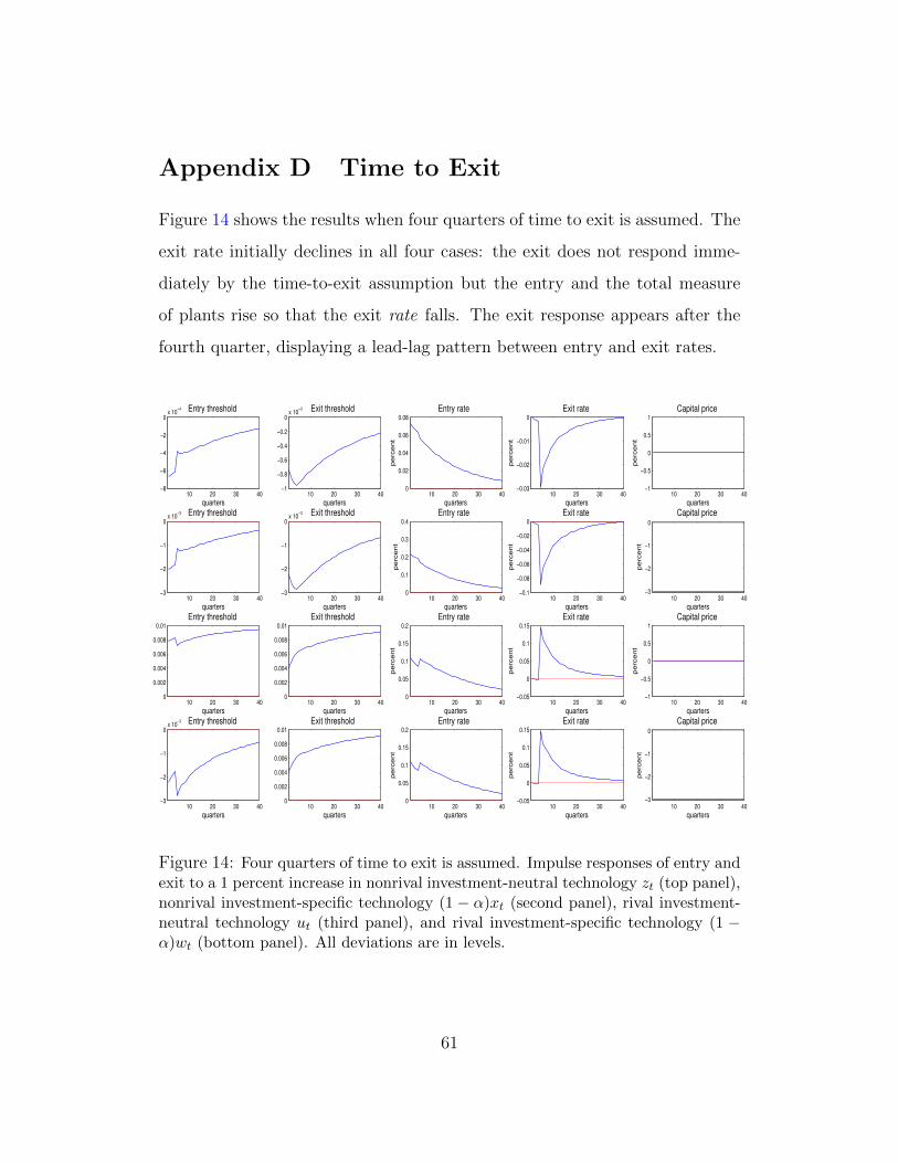
Appendix D Time to Exit
Figure 14 shows the results when four quarters of time to exit is assumed. The
exit rate initially declines in all four cases: the exit does not respond imme-
diately by the time-to-exit assumption but the entry and the total measure
of plants rise so that the exit rate falls. The exit response appears after the
fourth quarter, displaying a lead-lag pattern between entry and exit rates.
10 20 30 40−8
−6
−4
−2
0x 10
−4
quarters
Entry threshold
10 20 30 40−1
−0.8
−0.6
−0.4
−0.2
0x 10
−3
quarters
Exit threshold
10 20 30 400
0.02
0.04
0.06
0.08
pe
rce
nt
quarters
Entry rate
10 20 30 40−0.03
−0.02
−0.01
0
pe
rce
nt
quarters
Exit rate
10 20 30 40−1
−0.5
0
0.5
1
pe
rce
nt
quarters
Capital price
10 20 30 40−3
−2
−1
0x 10
−3
quarters
Entry threshold
10 20 30 40−3
−2
−1
0x 10
−3
quarters
Exit threshold
10 20 30 400
0.1
0.2
0.3
0.4
pe
rce
nt
quarters
Entry rate
10 20 30 40−0.1
−0.08
−0.06
−0.04
−0.02
0
pe
rce
nt
quarters
Exit rate
10 20 30 40−3
−2
−1
0
pe
rce
nt
quarters
Capital price
10 20 30 400
0.002
0.004
0.006
0.008
0.01
quarters
Entry threshold
10 20 30 400
0.002
0.004
0.006
0.008
0.01
quarters
Exit threshold
10 20 30 400
0.05
0.1
0.15
0.2
pe
rce
nt
quarters
Entry rate
10 20 30 40−0.05
0
0.05
0.1
0.15
pe
rce
nt
quarters
Exit rate
10 20 30 40−1
−0.5
0
0.5
1
pe
rce
nt
quarters
Capital price
10 20 30 40−3
−2
−1
0x 10
−3
quarters
Entry threshold
10 20 30 400
0.002
0.004
0.006
0.008
0.01
quarters
Exit threshold
10 20 30 400
0.05
0.1
0.15
0.2
pe
rce
nt
quarters
Entry rate
10 20 30 40−0.05
0
0.05
0.1
0.15
pe
rce
nt
quarters
Exit rate
10 20 30 40−3
−2
−1
0
pe
rce
nt
quarters
Capital price
Figure 14: Four quarters of time to exit is assumed. Impulse responses of entry andexit to a 1 percent increase in nonrival investment-neutral technology zt (top panel),nonrival investment-specific technology (1 − α)xt (second panel), rival investment-neutral technology ut (third panel), and rival investment-specific technology (1 −α)wt (bottom panel). All deviations are in levels.
61

Appendix E Data Summary Statistics
Figure 15: Data. Shaded areas indicate NBER recessions.
62

Variable Description Mean Std AC(1) AC(4)Corr
with ∆y
∆p log difference of investment price -1.32 0.61 0.46 0.02 -0.43
∆a log difference of labor productivity 0.30 0.70 -0.03 -0.08 0.36
h log of per capita hours -7.66 0.07 0.99 0.93 0.28
∆h log difference of per capita hours -0.08 0.77 0.71 0.27 0.61
enr establishment entry rate 3.22 0.25 0.87 0.78 0.36
exr establishment exit rate 2.94 0.20 0.79 0.57 -0.36
exr + enr establishment turnover rate 6.17 0.34 0.87 0.81 0.04
jcr job creation rate 7.20 0.81 0.92 0.93 0.45
jdr job destruction rate 6.91 0.68 0.94 0.76 -0.04
jcr + jdr job reallocation rate 14.10 1.35 0.96 0.97 0.25
tr1 acquisitions/lagged total assets 0.22 0.09 0.75 0.59 0.23
tr2 sales of PP&E/lagged total PP&E 0.45 0.14 0.87 0.77 0.16
tr1 + tr2 capital turnover rate 0.68 0.21 0.90 0.78 0.20
Table 4: Summary Statistics. Sample period is 1993:II–2014:II. The expressionAC(j) is the jth autocorrelation, ∆y is real per capital GDP growth, and PP&Estands for property, plant, and equipment. All variables are expressed as a percent-age except for log per capita hours h.
Appendix F Job Flow in the Manufacturing
Sector for 1972:I-1993:IV
Figure 16 shows that on impact, job destruction rate falls while job creation
rate slightly rises. As a result, job reallocation rate falls, which confirms the
finding of Michelacci and Lopez-Salido (2007). Note that the investment-
specific technology shock accounts for a small fraction of the job creation and
destruction rates in Figure 17. Not surprisingly, the correlation between the
reallocation shock and the investment-specific technology shock is low in this
sample.
63

5 10 15 20 25 30 35 40
−2
−1.5
−1
−0.5
0
Investment price
perc
ent
quarters5 10 15 20 25 30 35 40
−0.8
−0.7
−0.6
−0.5
−0.4
−0.3
−0.2
−0.1
0
0.1
0.2
Labor productivity
perc
ent
quarters5 10 15 20 25 30 35 40
0
0.2
0.4
0.6
0.8
1
1.2
1.4
1.6
Hours
perc
ent
quarters
5 10 15 20 25 30 35 40−0.2
−0.15
−0.1
−0.05
0
0.05
0.1
0.15
Job creation rate
perc
ent
quarters5 10 15 20 25 30 35 40
−0.4
−0.3
−0.2
−0.1
0
0.1
Job destruction rate
perc
ent
quarters5 10 15 20 25 30 35 40
−0.45
−0.4
−0.35
−0.3
−0.25
−0.2
−0.15
−0.1
−0.05
0
0.05
Job reallocation rate
perc
ent
quarters
Figure 16: Impulse responses to an investment-specific technology shock based onjob flow data in the manufacturing sector for 1972:I-1993:IV.
0 10 20 30 400
0.1
0.2
0.3
0.4
0.5
0.6
0.7
0.8
0.9
1
Investment price
fra
ctio
n o
f F
EV
quarters0 10 20 30 40
0
0.1
0.2
0.3
0.4
0.5
0.6
0.7
0.8
0.9
1
Labor productivity
fra
ctio
n o
f F
EV
quarters0 10 20 30 40
0
0.1
0.2
0.3
0.4
0.5
0.6
0.7
0.8
0.9
1
Hours
fra
ctio
n o
f F
EV
quarters
0 10 20 30 400
0.1
0.2
0.3
0.4
0.5
0.6
0.7
0.8
0.9
1
Job creation rate
fra
ctio
n o
f F
EV
quarters0 10 20 30 40
0
0.1
0.2
0.3
0.4
0.5
0.6
0.7
0.8
0.9
1
Job destruction rate
fra
ctio
n o
f F
EV
quarters0 10 20 30 40
0
0.1
0.2
0.3
0.4
0.5
0.6
0.7
0.8
0.9
1
Job reallocation rate
fra
ctio
n o
f F
EV
quarters
Figure 17: Fraction of forecast error variance (FEV) explained by investment-specific technology shock based on job flow data in the manufacturing sector for1972:I-1993:IV.
64

Appendix G Impulse Responses with 90 Per-
cent Error Bands
5 10 15 20 25 30 35 40
−5
−4
−3
−2
−1
0
Investment price
pe
rce
nt
quarters5 10 15 20 25 30 35 40
0
0.5
1
1.5
2
2.5
3
Labor productivity
pe
rce
nt
quarters5 10 15 20 25 30 35 40
−3
−2
−1
0
1
2
3
4
Hours
pe
rce
nt
quarters
5 10 15 20 25 30 35 40
−0.02
0
0.02
0.04
0.06
0.08
0.1
0.12
Entry rate
pe
rce
nt
quarters5 10 15 20 25 30 35 40
−0.08
−0.06
−0.04
−0.02
0
0.02
0.04
0.06
0.08
Exit rate
pe
rce
nt
quarters5 10 15 20 25 30 35 40
−0.05
0
0.05
0.1
0.15
Turnover rate
pe
rce
nt
quarters
Figure 18: Impulse responses to an investment-specific technology shock based onentry and exit data.
0 10 20 30 400
0.1
0.2
0.3
0.4
0.5
0.6
0.7
0.8
0.9
1
Investment price
fra
ctio
n o
f F
EV
quarters0 10 20 30 40
0
0.1
0.2
0.3
0.4
0.5
0.6
0.7
0.8
0.9
1
Labor productivity
fra
ctio
n o
f F
EV
quarters0 10 20 30 40
0
0.1
0.2
0.3
0.4
0.5
0.6
0.7
0.8
0.9
1
Hours
fra
ctio
n o
f F
EV
quarters
0 10 20 30 400
0.1
0.2
0.3
0.4
0.5
0.6
0.7
0.8
0.9
1
Entry rate
fra
ctio
n o
f F
EV
quarters0 10 20 30 40
0
0.1
0.2
0.3
0.4
0.5
0.6
0.7
0.8
0.9
1
Exit rate
fra
ctio
n o
f F
EV
quarters0 10 20 30 40
0
0.1
0.2
0.3
0.4
0.5
0.6
0.7
0.8
0.9
1
Turnover rate
fra
ctio
n o
f F
EV
quarters
Figure 19: Fraction of forecast error variance (FEV) explained by investment-specific technology shock based on entry and exit data
65

5 10 15 20 25 30 35 40
−2
−1.5
−1
−0.5
0
Investment price
pe
rce
nt
quarters5 10 15 20 25 30 35 40
−1
−0.8
−0.6
−0.4
−0.2
0
0.2
0.4
0.6
0.8
Labor productivity
pe
rce
nt
quarters5 10 15 20 25 30 35 40
0
0.5
1
1.5
2
2.5
3
3.5
4
4.5
5
Hours
pe
rce
nt
quarters
5 10 15 20 25 30 35 400
0.05
0.1
0.15
0.2
Job creation rate
pe
rce
nt
quarters5 10 15 20 25 30 35 40
−0.15
−0.1
−0.05
0
0.05
0.1
0.15
Job destruction rate
pe
rce
nt
quarters5 10 15 20 25 30 35 40
−0.05
0
0.05
0.1
0.15
0.2
0.25
0.3
Job reallocation rate
pe
rce
nt
quarters
Figure 20: Impulse responses to an investment-specific technology shock based onjob flow data.
0 10 20 30 400
0.1
0.2
0.3
0.4
0.5
0.6
0.7
0.8
0.9
1
Investment price
fra
ctio
n o
f F
EV
quarters0 10 20 30 40
0
0.1
0.2
0.3
0.4
0.5
0.6
0.7
0.8
0.9
1
Labor productivity
fra
ctio
n o
f F
EV
quarters0 10 20 30 40
0
0.1
0.2
0.3
0.4
0.5
0.6
0.7
0.8
0.9
1
Hours
fra
ctio
n o
f F
EV
quarters
0 10 20 30 400
0.1
0.2
0.3
0.4
0.5
0.6
0.7
0.8
0.9
1
Job creation rate
fra
ctio
n o
f F
EV
quarters0 10 20 30 40
0
0.1
0.2
0.3
0.4
0.5
0.6
0.7
0.8
0.9
1
Job destruction rate
fra
ctio
n o
f F
EV
quarters0 10 20 30 40
0
0.1
0.2
0.3
0.4
0.5
0.6
0.7
0.8
0.9
1
Job reallocation rate
fra
ctio
n o
f F
EV
quarters
Figure 21: Fraction of forecast error variance (FEV) explained by investment-specific technology shock based on job flow data.
66

5 10 15 20 25 30 35 40
−5
−4.5
−4
−3.5
−3
−2.5
−2
−1.5
−1
−0.5
0
Investment price
perc
ent
quarters5 10 15 20 25 30 35 40
0
0.5
1
1.5
2
2.5
3
Labor productivity
perc
ent
quarters5 10 15 20 25 30 35 40
−1.5
−1
−0.5
0
0.5
1
1.5
2
2.5
Hours
perc
ent
quarters
5 10 15 20 25 30 35 40
−0.01
−0.005
0
0.005
0.01
0.015
0.02
0.025
0.03
0.035
0.04
Acquisitions turnover rate
perc
ent
quarters5 10 15 20 25 30 35 40
−0.01
0
0.01
0.02
0.03
0.04
0.05
0.06
Property sale turnover rate
perc
ent
quarters5 10 15 20 25 30 35 40
−0.02
0
0.02
0.04
0.06
0.08
0.1
Sum of turnover rates
perc
ent
quarters
Figure 22: Impulse responses to an investment-specific technology shock based oncapital reallocation data.
0 10 20 30 400
0.1
0.2
0.3
0.4
0.5
0.6
0.7
0.8
0.9
1
Investment price
frac
tion
of F
EV
quarters0 10 20 30 40
0
0.1
0.2
0.3
0.4
0.5
0.6
0.7
0.8
0.9
1
Labor productivity
frac
tion
of F
EV
quarters0 10 20 30 40
0
0.1
0.2
0.3
0.4
0.5
0.6
0.7
0.8
0.9
1
Hours
frac
tion
of F
EV
quarters
0 10 20 30 400
0.1
0.2
0.3
0.4
0.5
0.6
0.7
0.8
0.9
1
Acquisitions turnover rate
frac
tion
of F
EV
quarters0 10 20 30 40
0
0.1
0.2
0.3
0.4
0.5
0.6
0.7
0.8
0.9
1
Property sale turnover rate
frac
tion
of F
EV
quarters0 10 20 30 40
0
0.1
0.2
0.3
0.4
0.5
0.6
0.7
0.8
0.9
1
Sum of turnover rates
frac
tion
of F
EV
quarters
Figure 23: Fraction of forecast error variance (FEV) explained by investment-specific technology shock based on capital reallocation data.
67
Recommended