Linear Programming ModelLinear Programming ModelLinear Programming ModelLinear Programming Model
TBS910 BUSINESS ANALYTICSTBS910 BUSINESS ANALYTICS
byProf.Stephen Ong
Visiting Professor, Shenzhen University
Visiting Fellow, Sydney Business School, University of Wollongong
Today’s Overview Today’s Overview
7-3
Learning ObjectivesLearning Objectives
1.1. Understand the basic assumptions and properties of Understand the basic assumptions and properties of linear programming (LP).linear programming (LP).
2.2. Graphically solve any LP problem that has only two Graphically solve any LP problem that has only two variables by both the corner point and isoprofit line variables by both the corner point and isoprofit line methods.methods.
3.3. Understand special issues in LP such as Understand special issues in LP such as infeasibility, unboundedness, redundancy, and infeasibility, unboundedness, redundancy, and alternative optimal solutions.alternative optimal solutions.
4.4. Understand the role of sensitivity analysis.Understand the role of sensitivity analysis.
5.5. Use Excel spreadsheets to solve LP problems.Use Excel spreadsheets to solve LP problems.
After this lecture, students will be able to:After this lecture, students will be able to:
7-4
OutlineOutline7.17.1 IntroductionIntroduction7.27.2 Requirements of a Linear Programming Requirements of a Linear Programming
ProblemProblem7.37.3 Formulating LP ProblemsFormulating LP Problems7.47.4 Graphical Solution to an LP ProblemGraphical Solution to an LP Problem7.57.5 Solving Flair Furniture’s LP Problem Solving Flair Furniture’s LP Problem
using QM for Windows and Excelusing QM for Windows and Excel7.67.6 Solving Minimization ProblemsSolving Minimization Problems7.77.7 Four Special Cases in LPFour Special Cases in LP7.87.8 Sensitivity AnalysisSensitivity Analysis
7-5
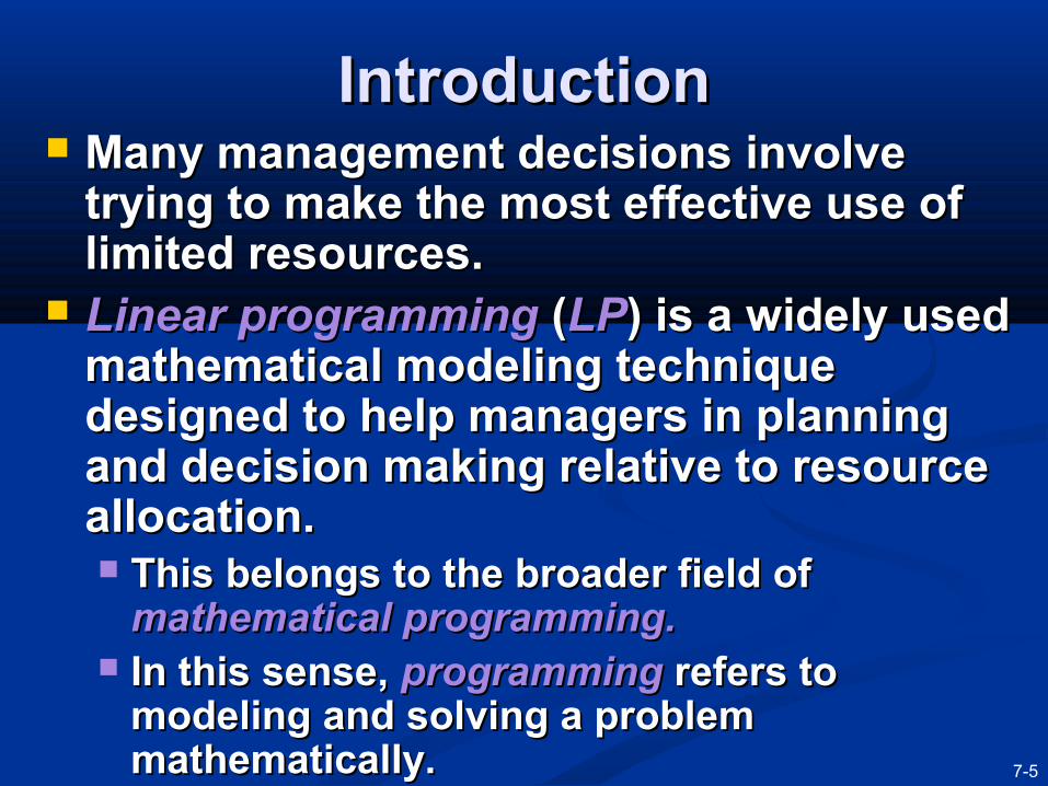
IntroductionIntroduction Many management decisions involve Many management decisions involve
trying to make the most effective use of trying to make the most effective use of limited resources.limited resources.
Linear programmingLinear programming ( (LPLP) is a widely used ) is a widely used mathematical modeling technique mathematical modeling technique designed to help managers in planning designed to help managers in planning and decision making relative to resource and decision making relative to resource allocation.allocation. This belongs to the broader field of This belongs to the broader field of
mathematical programming.mathematical programming. In this sense, In this sense, programmingprogramming refers to refers to
modeling and solving a problem modeling and solving a problem mathematically.mathematically.
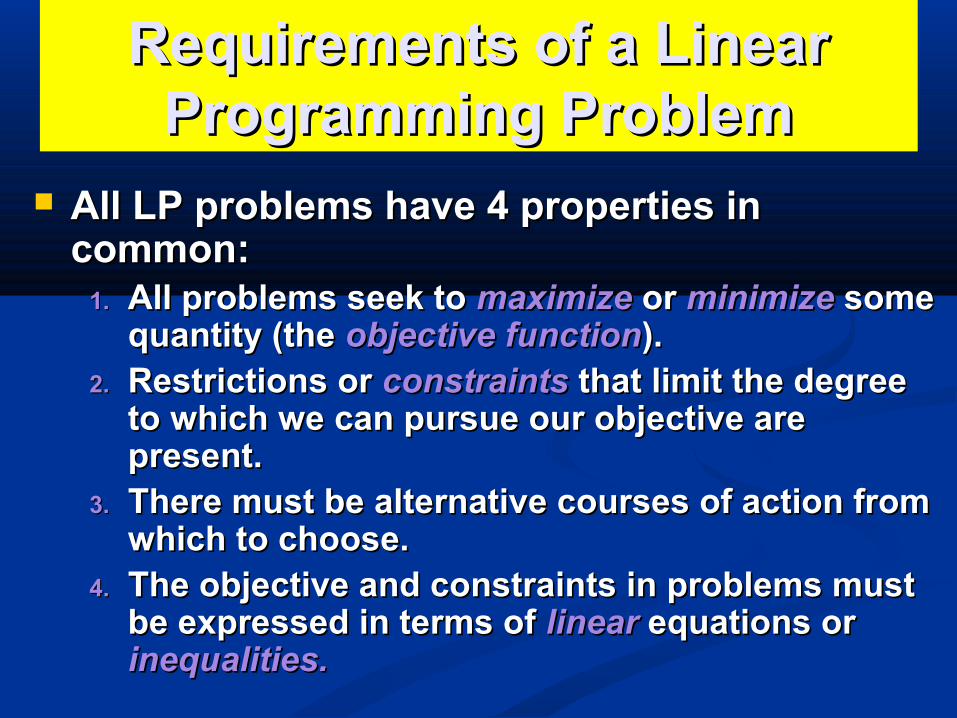
Requirements of a Linear Requirements of a Linear Programming ProblemProgramming Problem
All LP problems have 4 properties in All LP problems have 4 properties in common:common:
1.1. All problems seek to All problems seek to maximizemaximize or or minimizeminimize some some quantity (the quantity (the objective functionobjective function).).
2.2. Restrictions or Restrictions or constraintsconstraints that limit the degree that limit the degree to which we can pursue our objective are to which we can pursue our objective are present.present.
3.3. There must be alternative courses of action from There must be alternative courses of action from which to choose.which to choose.
4.4. The objective and constraints in problems must The objective and constraints in problems must be expressed in terms of be expressed in terms of linearlinear equations or equations or inequalities.inequalities.
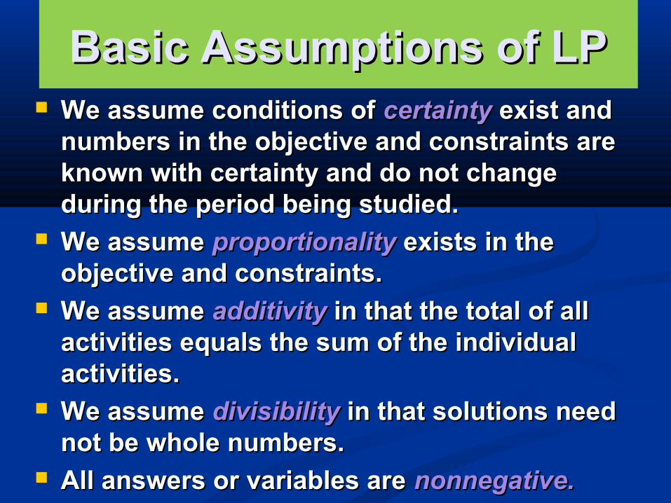
Basic Assumptions of LPBasic Assumptions of LP We assume conditions of We assume conditions of certaintycertainty exist and exist and
numbers in the objective and constraints are numbers in the objective and constraints are known with certainty and do not change known with certainty and do not change during the period being studied.during the period being studied.
We assume We assume proportionalityproportionality exists in the exists in the objective and constraints.objective and constraints.
We assume We assume additivityadditivity in that the total of all in that the total of all activities equals the sum of the individual activities equals the sum of the individual activities.activities.
We assume We assume divisibilitydivisibility in that solutions need in that solutions need not be whole numbers.not be whole numbers.
All answers or variables are All answers or variables are nonnegative.nonnegative.
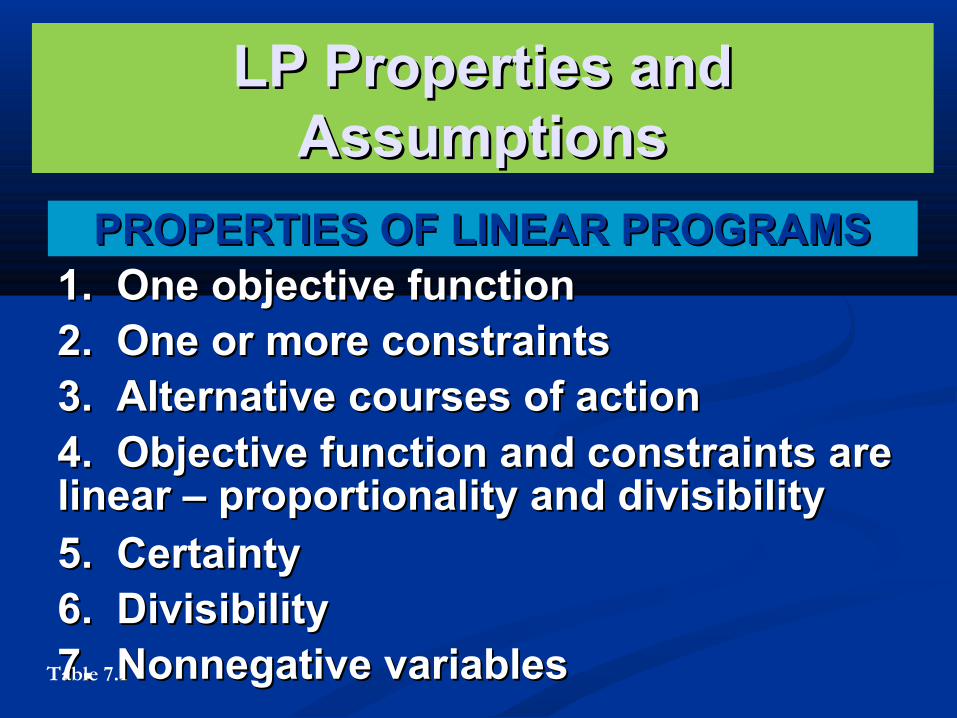
LP Properties and LP Properties and AssumptionsAssumptions
PROPERTIES OF LINEAR PROGRAMSPROPERTIES OF LINEAR PROGRAMS1. One objective function1. One objective function2. One or more constraints2. One or more constraints3. Alternative courses of action3. Alternative courses of action4. Objective function and constraints are 4. Objective function and constraints are linear – proportionality and divisibilitylinear – proportionality and divisibility
5. Certainty5. Certainty6. Divisibility6. Divisibility7. Nonnegative variables7. Nonnegative variablesTable 7.1
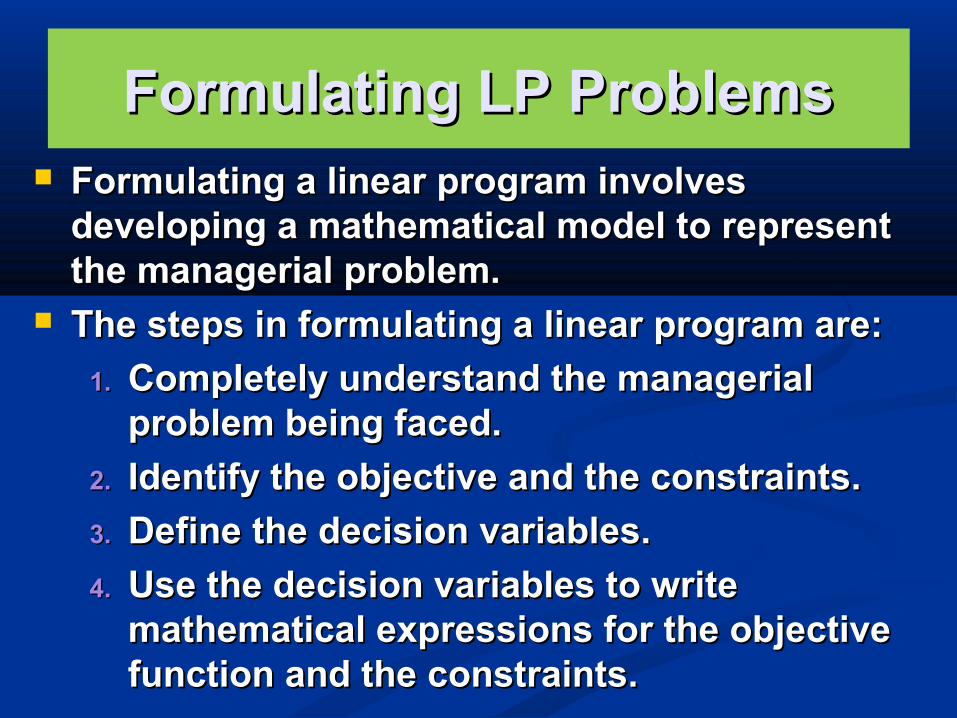
Formulating LP ProblemsFormulating LP Problems Formulating a linear program involves Formulating a linear program involves
developing a mathematical model to represent developing a mathematical model to represent the managerial problem.the managerial problem.
The steps in formulating a linear program are:The steps in formulating a linear program are:
1.1. Completely understand the managerial Completely understand the managerial problem being faced.problem being faced.
2.2. Identify the objective and the constraints.Identify the objective and the constraints.
3.3. Define the decision variables.Define the decision variables.
4.4. Use the decision variables to write Use the decision variables to write mathematical expressions for the objective mathematical expressions for the objective function and the constraints.function and the constraints.
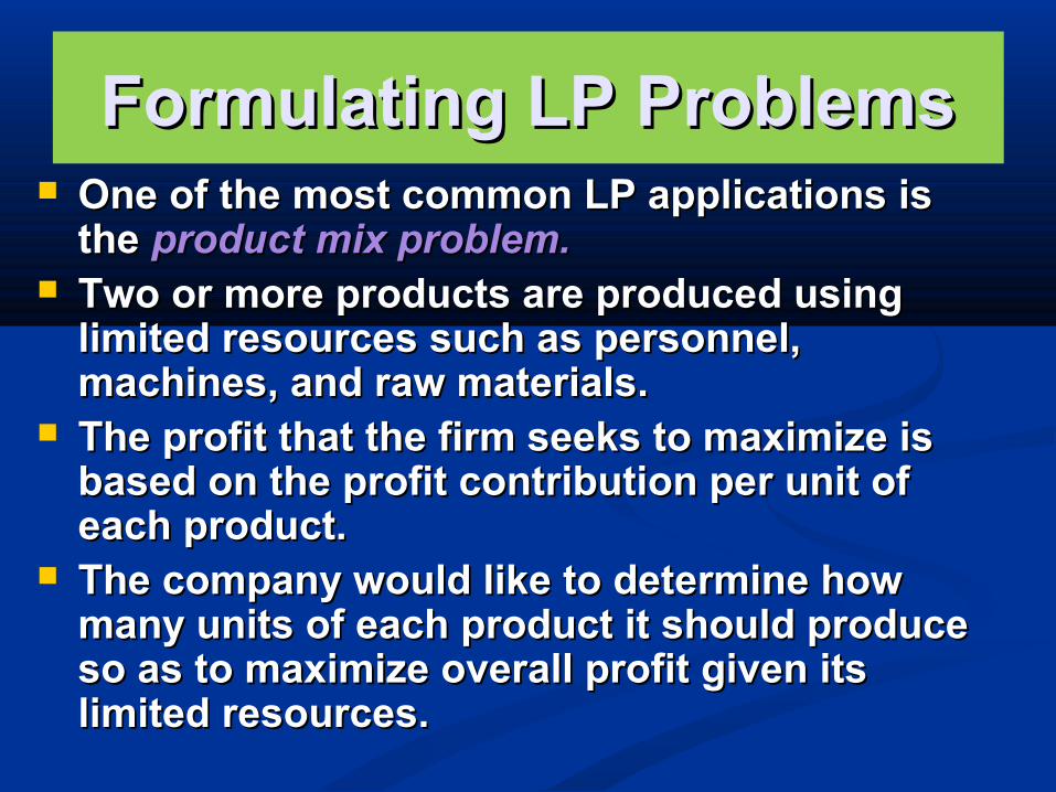
Formulating LP ProblemsFormulating LP Problems One of the most common LP applications is One of the most common LP applications is
the the product mix problem.product mix problem. Two or more products are produced using Two or more products are produced using
limited resources such as personnel, limited resources such as personnel, machines, and raw materials.machines, and raw materials.
The profit that the firm seeks to maximize is The profit that the firm seeks to maximize is based on the profit contribution per unit of based on the profit contribution per unit of each product.each product.
The company would like to determine how The company would like to determine how many units of each product it should produce many units of each product it should produce so as to maximize overall profit given its so as to maximize overall profit given its limited resources.limited resources.
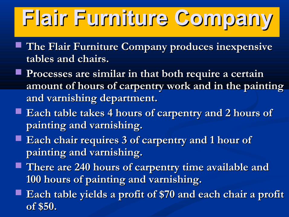
Flair Furniture CompanyFlair Furniture Company The Flair Furniture Company produces inexpensive The Flair Furniture Company produces inexpensive
tables and chairs.tables and chairs. Processes are similar in that both require a certain Processes are similar in that both require a certain
amount of hours of carpentry work and in the painting amount of hours of carpentry work and in the painting and varnishing department.and varnishing department.
Each table takes 4 hours of carpentry and 2 hours of Each table takes 4 hours of carpentry and 2 hours of painting and varnishing.painting and varnishing.
Each chair requires 3 of carpentry and 1 hour of Each chair requires 3 of carpentry and 1 hour of painting and varnishing.painting and varnishing.
There are 240 hours of carpentry time available and There are 240 hours of carpentry time available and 100 hours of painting and varnishing.100 hours of painting and varnishing.
Each table yields a profit of $70 and each chair a profit Each table yields a profit of $70 and each chair a profit of $50.of $50.
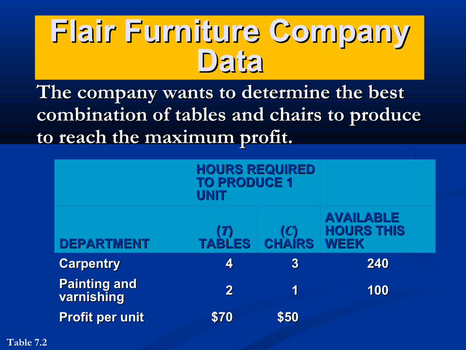
Flair Furniture Company Flair Furniture Company DataData
The company wants to determine the best The company wants to determine the best combination of tables and chairs to produce combination of tables and chairs to produce to reach the maximum profit.to reach the maximum profit.
HOURS REQUIRED HOURS REQUIRED TO PRODUCE 1 TO PRODUCE 1 UNITUNIT
DEPARTMENTDEPARTMENT((TT) )
TABLESTABLES((CC) )
CHAIRSCHAIRS
AVAILABLE AVAILABLE HOURS THIS HOURS THIS WEEKWEEK
CarpentryCarpentry 44 33 240240
Painting and Painting and varnishingvarnishing 22 11 100100
Profit per unitProfit per unit $70$70 $50$50
Table 7.2
Flair Furniture CompanyFlair Furniture Company
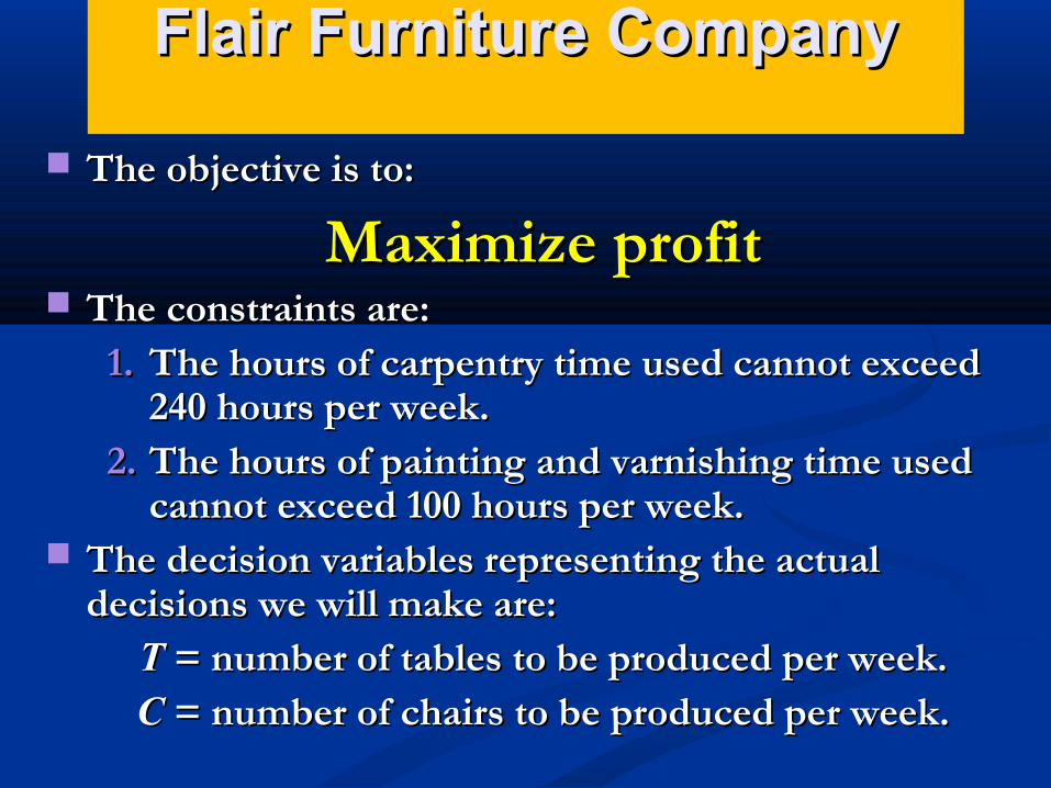
The objective is to:The objective is to:
Maximize profitMaximize profit The constraints are:The constraints are:
1.1. The hours of carpentry time used cannot exceed The hours of carpentry time used cannot exceed 240 hours per week.240 hours per week.
2.2. The hours of painting and varnishing time used The hours of painting and varnishing time used cannot exceed 100 hours per week.cannot exceed 100 hours per week.
The decision variables representing the actual The decision variables representing the actual decisions we will make are:decisions we will make are:
TT = number of tables to be produced per week. = number of tables to be produced per week.CC = number of chairs to be produced per week. = number of chairs to be produced per week.
7-14
Flair Furniture CompanyFlair Furniture Company
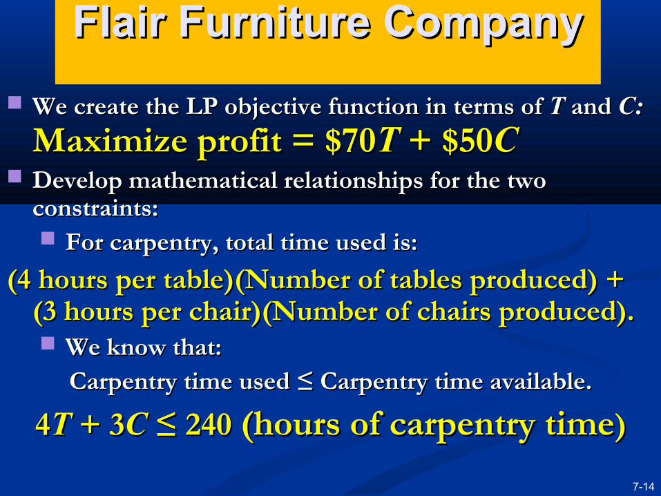
We create the LP objective function in terms of We create the LP objective function in terms of TT and and C: C:
Maximize profit = $70Maximize profit = $70TT + $50 + $50CC Develop mathematical relationships for the two Develop mathematical relationships for the two
constraints:constraints: For carpentry, total time used is:For carpentry, total time used is:
(4 hours per table)(Number of tables produced) + (4 hours per table)(Number of tables produced) + (3 hours per chair)(Number of chairs produced).(3 hours per chair)(Number of chairs produced). We know that:We know that:
Carpentry time used Carpentry time used ≤ Carpentry time available.≤ Carpentry time available.
44TT + 3 + 3CC ≤ 240 ≤ 240 (hours of carpentry time(hours of carpentry time))
Flair Furniture CompanyFlair Furniture Company
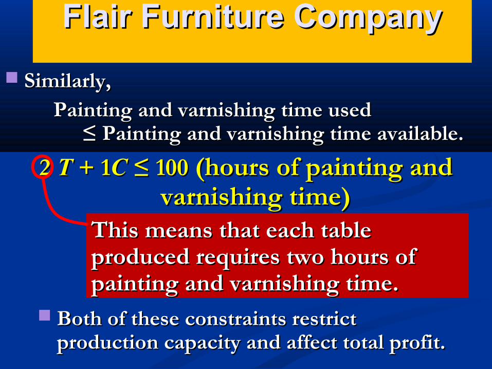
Similarly,Similarly,Painting and varnishing time used Painting and varnishing time used
≤ Painting and varnishing time available.≤ Painting and varnishing time available.
2 2 TT + 1 + 1CC ≤ 100 ≤ 100 (hours of painting and (hours of painting and varnishing time)varnishing time)
This means that each table This means that each table produced requires two hours of produced requires two hours of painting and varnishing time.painting and varnishing time.
Both of these constraints restrict Both of these constraints restrict production capacity and affect total profit.production capacity and affect total profit.
Flair Furniture CompanyFlair Furniture Company
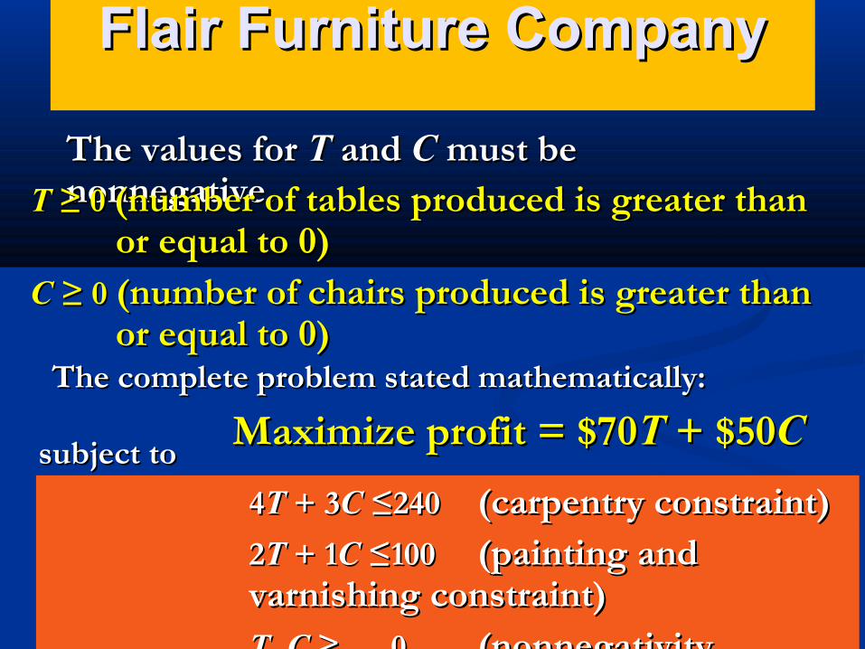
The values for The values for TT and and CC must be must be nonnegative.nonnegative.TT ≥ 0 ≥ 0 (number of tables produced is greater than (number of tables produced is greater than
or equal to 0)or equal to 0)CC ≥ 0 ≥ 0 (number of chairs produced is greater than (number of chairs produced is greater than
or equal to 0)or equal to 0)The complete problem stated mathematically:The complete problem stated mathematically:
Maximize profit = $70Maximize profit = $70TT + $50 + $50CCsubject tosubject to
44TT + 3+ 3CC ≤240 ≤240 (carpentry constraint)(carpentry constraint)22TT + 1 + 1CC ≤ ≤100100 (painting and (painting and varnishing constraint)varnishing constraint)TT, , CC ≥≥ 00 (nonnegativity (nonnegativity constraint)constraint)
Graphical Solution to an LP Graphical Solution to an LP ProblemProblem
The easiest way to solve a small LP The easiest way to solve a small LP problems is graphically.problems is graphically.
The graphical method only works when The graphical method only works when there are just two decision variables. there are just two decision variables.
When there are more than two variables, When there are more than two variables, a more complex approach is needed as it a more complex approach is needed as it is not possible to plot the solution on a is not possible to plot the solution on a two-dimensional graph.two-dimensional graph.
The graphical method provides valuable The graphical method provides valuable insight into how other approaches work.insight into how other approaches work.
Graphical Representation of a Graphical Representation of a ConstraintConstraint
100 –
–
80 –
–
60 –
–
40 –
–
20 –
–
–
C
| | | | | | | | | | | |
0 20 40 60 80 100 T
Num
ber
of C
hair
sN
umbe
r of
Cha
irs
Number of TablesNumber of Tables
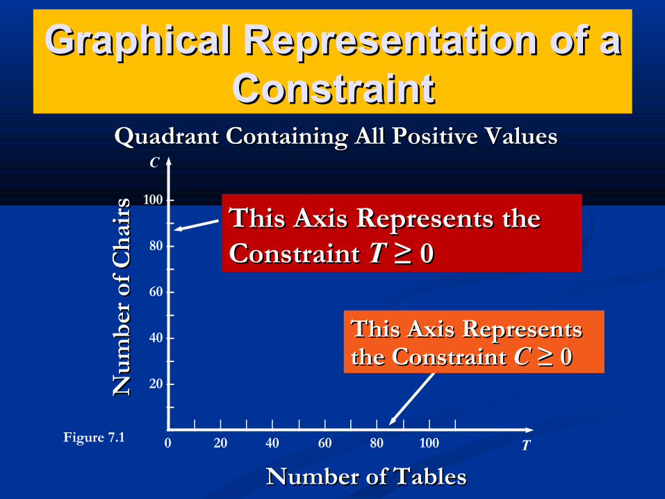
This Axis Represents the This Axis Represents the Constraint Constraint TT ≥ 0≥ 0
This Axis Represents This Axis Represents the Constraint the Constraint CC ≥ 0≥ 0
Figure 7.1
Quadrant Containing All Positive ValuesQuadrant Containing All Positive Values
Graphical Representation of a Graphical Representation of a ConstraintConstraint
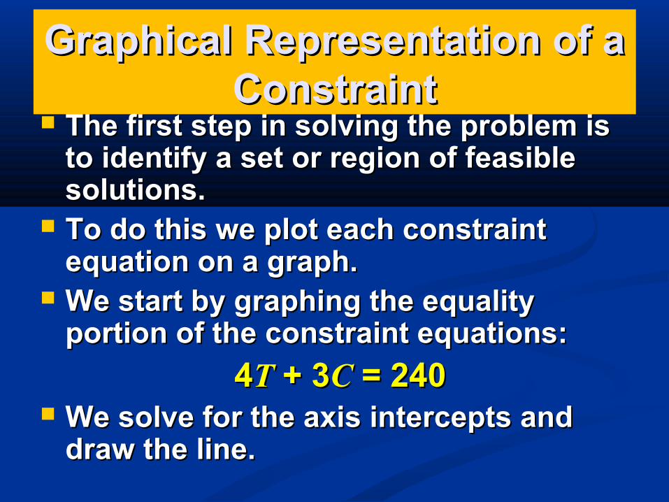
The first step in solving the problem is The first step in solving the problem is to identify a set or region of feasible to identify a set or region of feasible solutions.solutions.
To do this we plot each constraint To do this we plot each constraint equation on a graph.equation on a graph.
We start by graphing the equality We start by graphing the equality portion of the constraint equations:portion of the constraint equations:
44TT + 3 + 3CC = 240 = 240 We solve for the axis intercepts and We solve for the axis intercepts and
draw the line.draw the line.
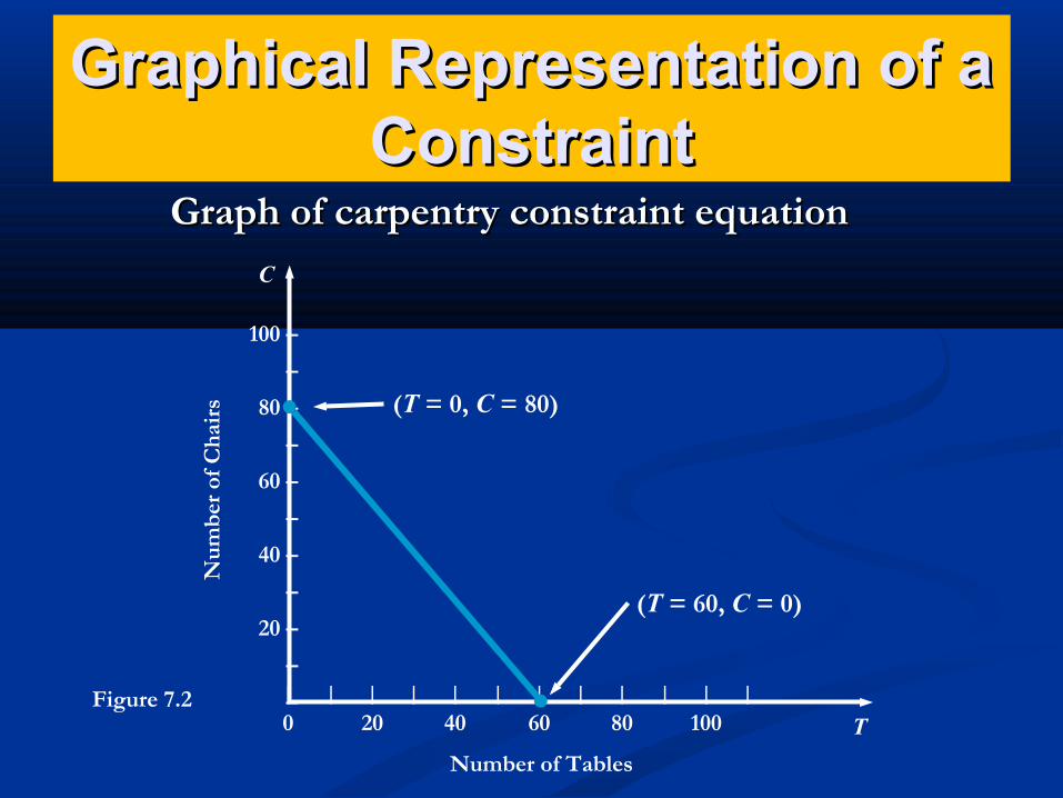
Graphical Representation of a Graphical Representation of a ConstraintConstraint
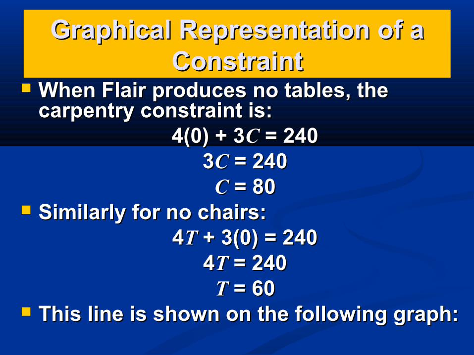
When Flair produces no tables, the When Flair produces no tables, the carpentry constraint is:carpentry constraint is:
4(0) + 34(0) + 3CC = 240 = 24033CC = 240 = 240
CC = 80 = 80 Similarly for no chairs:Similarly for no chairs:
44TT + 3(0) = 240 + 3(0) = 24044TT = 240 = 240
TT = 60 = 60 This line is shown on the following graph:This line is shown on the following graph:
Graphical Representation of a Graphical Representation of a ConstraintConstraint
100 –
–
80 –
–
60 –
–
40 –
–
20 –
–
–
C
| | | | | | | | | | | |
0 20 40 60 80 100 T
Num
ber
of C
hair
s
Number of Tables
(T = 0, C = 80)
Figure 7.2
(T = 60, C = 0)
Graph of carpentry constraint equationGraph of carpentry constraint equation
7-22
Graphical Representation of a Graphical Representation of a ConstraintConstraint
100 –
–
80 –
–
60 –
–
40 –
–
20 –
–
–
C
| | | | | | | | | | | |
0 20 40 60 80 100 T
Num
ber
of C
hair
sN
umbe
r of
Cha
irs
Number of TablesNumber of Tables
Figure 7.3
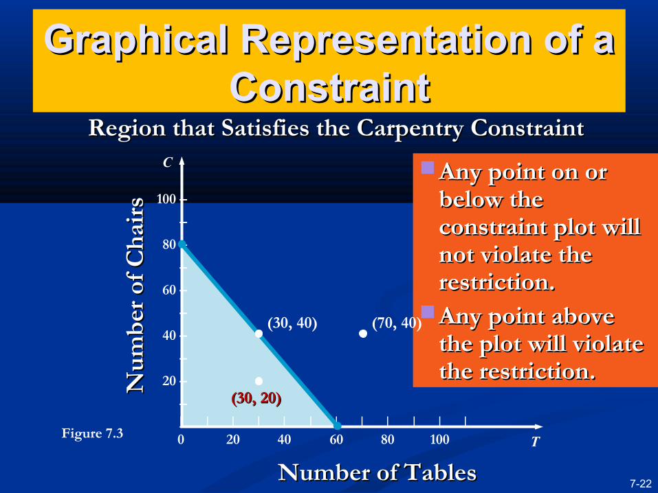
Any point on or Any point on or below the below the constraint plot will constraint plot will not violate the not violate the restriction.restriction.
Any point above Any point above the plot will violate the plot will violate the restriction.the restriction.
(30, 40)
(30, 20)(30, 20)
(70, 40)
Region that Satisfies the Carpentry ConstraintRegion that Satisfies the Carpentry Constraint
Graphical Representation of a Graphical Representation of a ConstraintConstraint
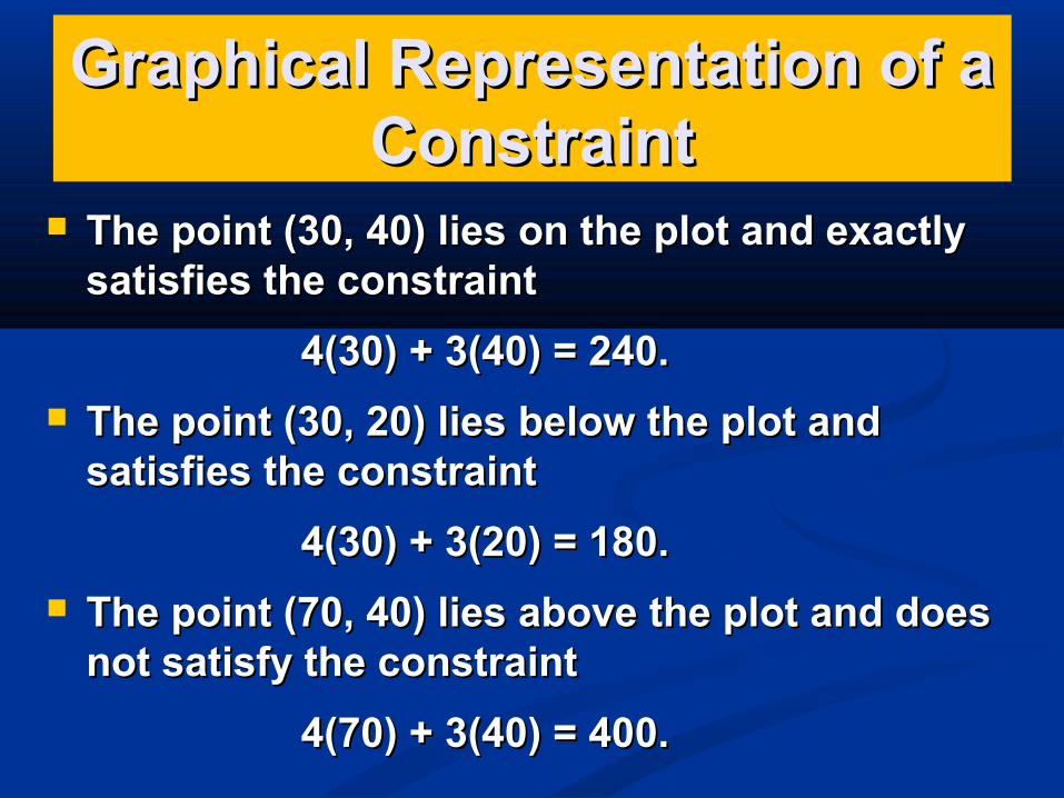
The point (30, 40) lies on the plot and exactly The point (30, 40) lies on the plot and exactly satisfies the constraintsatisfies the constraint
4(30) + 3(40) = 240.4(30) + 3(40) = 240.
The point (30, 20) lies below the plot and The point (30, 20) lies below the plot and satisfies the constraintsatisfies the constraint
4(30) + 3(20) = 180.4(30) + 3(20) = 180.
The point (70, 40) lies above the plot and does The point (70, 40) lies above the plot and does not satisfy the constraintnot satisfy the constraint
4(70) + 3(40) = 400.4(70) + 3(40) = 400.
Graphical Representation of a Graphical Representation of a ConstraintConstraint
100 –
–
80 –
–
60 –
–
40 –
–
20 –
–
–
C
| | | | | | | | | | | |
0 20 40 60 80 100 T
Num
ber
of C
hair
s
Number of Tables
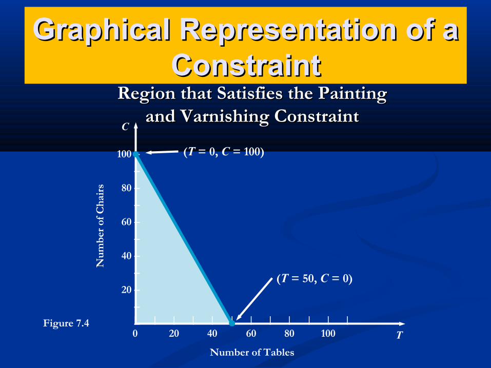
(T = 0, C = 100)
Figure 7.4
(T = 50, C = 0)
Region that Satisfies the Painting Region that Satisfies the Painting and Varnishing Constraintand Varnishing Constraint
Graphical Representation of a Graphical Representation of a ConstraintConstraint
To produce tables and chairs, both To produce tables and chairs, both departments must be used.departments must be used.
We need to find a solution that satisfies both We need to find a solution that satisfies both constraints constraints simultaneously.simultaneously.
A new graph shows both constraint plots.A new graph shows both constraint plots. The The feasible regionfeasible region (or (or area of feasible area of feasible
solutionssolutions) is where all constraints are ) is where all constraints are satisfied.satisfied.
Any point inside this region is a Any point inside this region is a feasiblefeasible solution.solution.
Any point outside the region is an Any point outside the region is an infeasibleinfeasible solution.solution.
Graphical Representation of a Graphical Representation of a ConstraintConstraint
100 –
–
80 –
–
60 –
–
40 –
–
20 –
–
–
C
| | | | | | | | | | | |
0 20 40 60 80 100 T
Num
ber
of C
hair
sN
umbe
r of
Cha
irs
Number of Tables
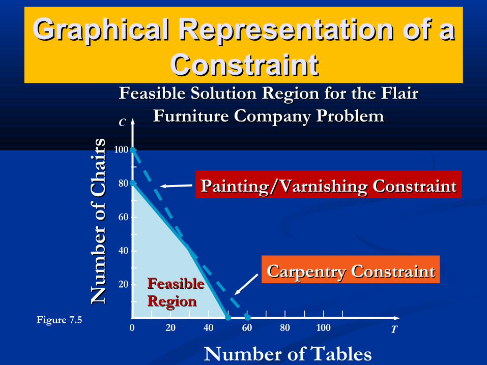
Figure 7.5
Feasible Solution Region for the Flair Feasible Solution Region for the Flair Furniture Company ProblemFurniture Company Problem
Painting/Varnishing ConstraintPainting/Varnishing Constraint
Carpentry ConstraintCarpentry ConstraintFeasible Feasible RegionRegion
Graphical Representation of a Graphical Representation of a ConstraintConstraint
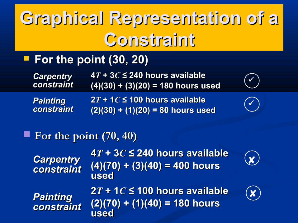
For the point (30, 20)For the point (30, 20)Carpentry Carpentry constraintconstraint
44TT + 3 + 3CC ≤ 240 hours available ≤ 240 hours available(4)(30) + (3)(20) = 180 hours used(4)(30) + (3)(20) = 180 hours used
Painting Painting constraintconstraint
22TT + 1 + 1CC ≤ 100 hours available ≤ 100 hours available(2)(30) + (1)(20) = 80 hours used(2)(30) + (1)(20) = 80 hours used
For the point (70, 40)For the point (70, 40)
Carpentry Carpentry constraintconstraint
44TT + 3 + 3CC ≤ 240 hours available ≤ 240 hours available(4)(70) + (3)(40) = 400 hours (4)(70) + (3)(40) = 400 hours usedused
Painting Painting constraintconstraint
22TT + 1 + 1CC ≤ 100 hours available ≤ 100 hours available(2)(70) + (1)(40) = 180 hours (2)(70) + (1)(40) = 180 hours usedused
Graphical Representation of a Graphical Representation of a ConstraintConstraint
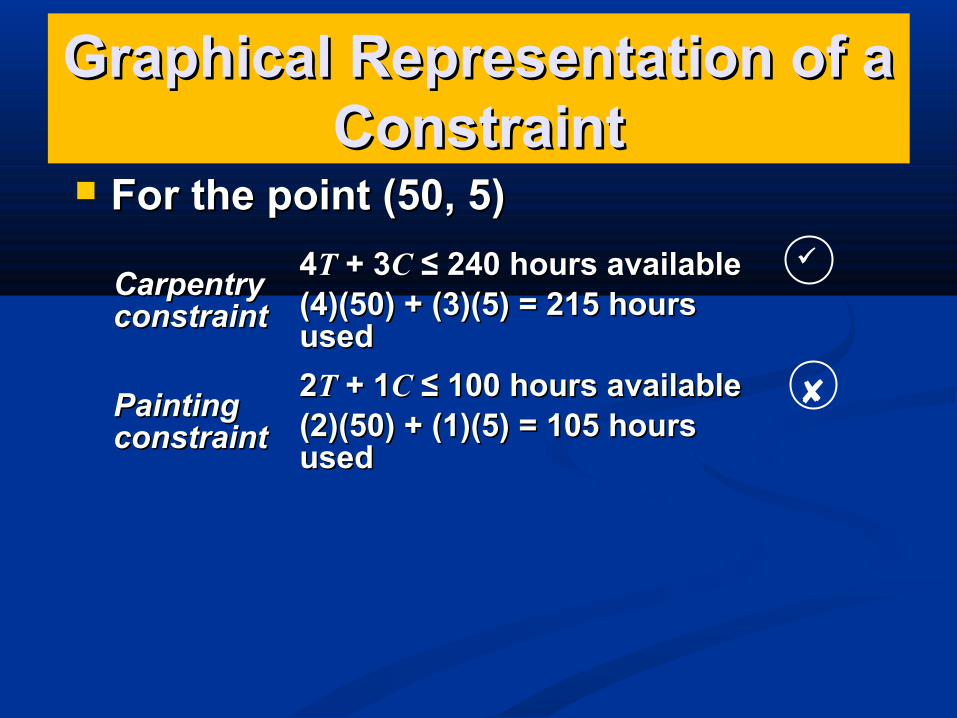
For the point (50, 5)For the point (50, 5)
Carpentry Carpentry constraintconstraint
44TT + 3 + 3CC ≤ 240 hours available ≤ 240 hours available(4)(50) + (3)(5) = 215 hours (4)(50) + (3)(5) = 215 hours usedused
Painting Painting constraintconstraint
22TT + 1 + 1CC ≤ 100 hours available ≤ 100 hours available(2)(50) + (1)(5) = 105 hours (2)(50) + (1)(5) = 105 hours usedused
Isoprofit Line Solution Isoprofit Line Solution MethodMethod
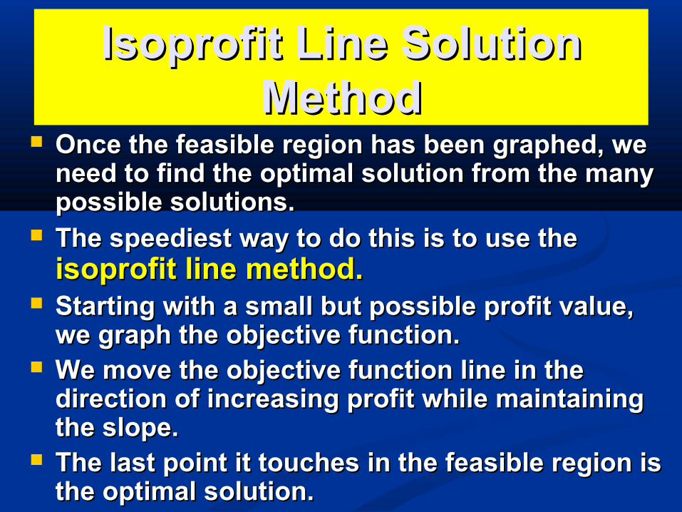
Once the feasible region has been graphed, we Once the feasible region has been graphed, we need to find the optimal solution from the many need to find the optimal solution from the many possible solutions.possible solutions.
The speediest way to do this is to use the The speediest way to do this is to use the isoprofit line method.isoprofit line method.
Starting with a small but possible profit value, Starting with a small but possible profit value, we graph the objective function.we graph the objective function.
We move the objective function line in the We move the objective function line in the direction of increasing profit while maintaining direction of increasing profit while maintaining the slope.the slope.
The last point it touches in the feasible region is The last point it touches in the feasible region is the optimal solution.the optimal solution.
Isoprofit Line Solution Isoprofit Line Solution MethodMethod
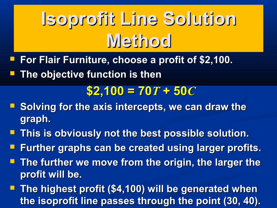
For Flair Furniture, choose a profit of $2,100.For Flair Furniture, choose a profit of $2,100. The objective function is thenThe objective function is then
$2,100 = 70$2,100 = 70TT + 50 + 50CC Solving for the axis intercepts, we can draw the Solving for the axis intercepts, we can draw the
graph.graph. This is obviously not the best possible solution.This is obviously not the best possible solution. Further graphs can be created using larger profits.Further graphs can be created using larger profits. The further we move from the origin, the larger the The further we move from the origin, the larger the
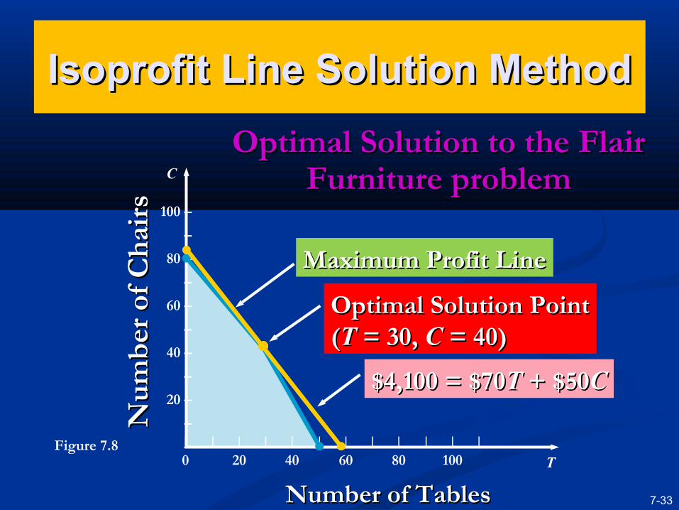
profit will be.profit will be. The highest profit ($4,100) will be generated when The highest profit ($4,100) will be generated when
the isoprofit line passes through the point (30, 40).the isoprofit line passes through the point (30, 40).
100 –
–
80 –
–
60 –
–
40 –
–
20 –
–
–
C
| | | | | | | | | | | |
0 20 40 60 80 100 T
Num
ber
of C
hair
sN
umbe
r of
Cha
irs
Number of TablesNumber of Tables
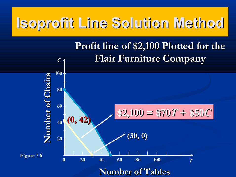
Figure 7.6
Profit line of $2,100 Plotted for the Profit line of $2,100 Plotted for the Flair Furniture CompanyFlair Furniture Company
$2,100 = $70$2,100 = $70TT + $50 + $50CC
(30, 0)(30, 0)
(0, 42)(0, 42)
Isoprofit Line Solution MethodIsoprofit Line Solution Method
100 –
–
80 –
–
60 –
–
40 –
–
20 –
–
–
C
| | | | | | | | | | | |
0 20 40 60 80 100 T
Num
ber
of C
hair
s
Number of Tables
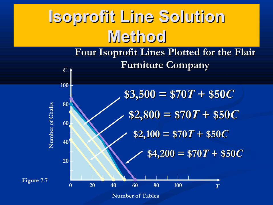
Figure 7.7
Four Isoprofit Lines Plotted for the Flair Four Isoprofit Lines Plotted for the Flair Furniture CompanyFurniture Company
$2,100 = $70$2,100 = $70TT + $50 + $50CC
$2,800 = $70$2,800 = $70TT + $50 + $50CC
$3,500 = $70$3,500 = $70TT + $50 + $50CC
$4,200 = $70$4,200 = $70TT + $50 + $50CC
Isoprofit Line Solution Isoprofit Line Solution MethodMethod
7-33
100 –
–
80 –
–
60 –
–
40 –
–
20 –
–
–
C
| | | | | | | | | | | |
0 20 40 60 80 100 T
Num
ber
of C
hair
sN
umbe
r of
Cha
irs
Number of TablesNumber of Tables
Figure 7.8
Optimal Solution to the Flair Optimal Solution to the Flair Furniture problemFurniture problem
Optimal Solution PointOptimal Solution Point((TT = 30, = 30, CC = 40) = 40)
Maximum Profit LineMaximum Profit Line
$4,100 = $70$4,100 = $70TT + $50 + $50CC
Isoprofit Line Solution MethodIsoprofit Line Solution Method
7-34
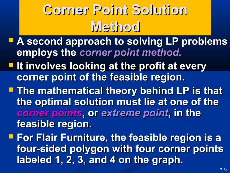
A second approach to solving LP problems A second approach to solving LP problems employs the employs the corner point method.corner point method.
It involves looking at the profit at every It involves looking at the profit at every corner point of the feasible region.corner point of the feasible region.
The mathematical theory behind LP is that The mathematical theory behind LP is that the optimal solution must lie at one of the the optimal solution must lie at one of the corner pointscorner points, or , or extreme pointextreme point, in the , in the feasible region.feasible region.
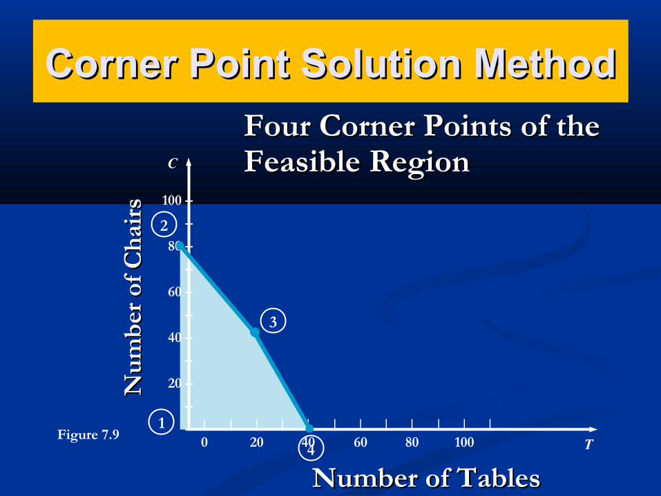
For Flair Furniture, the feasible region is a For Flair Furniture, the feasible region is a four-sided polygon with four corner points four-sided polygon with four corner points labeled 1, 2, 3, and 4 on the graph.labeled 1, 2, 3, and 4 on the graph.
Corner Point Solution Corner Point Solution MethodMethod
100 –
–
80 –
–
60 –
–
40 –
–
20 –
–
–
C
| | | | | | | | | | | |
0 20 40 60 80 100 T
Num
ber
of C
hair
sN
umbe
r of
Cha
irs
Number of TablesNumber of Tables
Figure 7.9
Four Corner Points of the Four Corner Points of the Feasible RegionFeasible Region
1
2
3
4
Corner Point Solution MethodCorner Point Solution Method
Corner Point Solution MethodCorner Point Solution Method
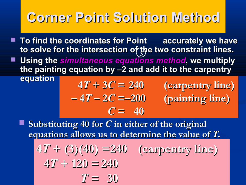
To find the coordinates for Point accurately we have To find the coordinates for Point accurately we have to solve for the intersection of the two constraint lines.to solve for the intersection of the two constraint lines.
Using the Using the simultaneous equations methodsimultaneous equations method, we multiply , we multiply the painting equation by –2 and add it to the carpentry the painting equation by –2 and add it to the carpentry equationequation
44TT + 3 + 3CC = = 240240 (carpentry line)(carpentry line)– – 44TT – 2 – 2CC = =––200200 (painting line)(painting line)
CC = = 4040 Substituting 40 for Substituting 40 for CC in either of the original in either of the original
equations allows us to determine the value of equations allows us to determine the value of T.T.
44TT + (3)(40) = + (3)(40) =240240 (carpentry line)(carpentry line)44TT + 120 = + 120 = 240240
TT = = 3030
3
7-37
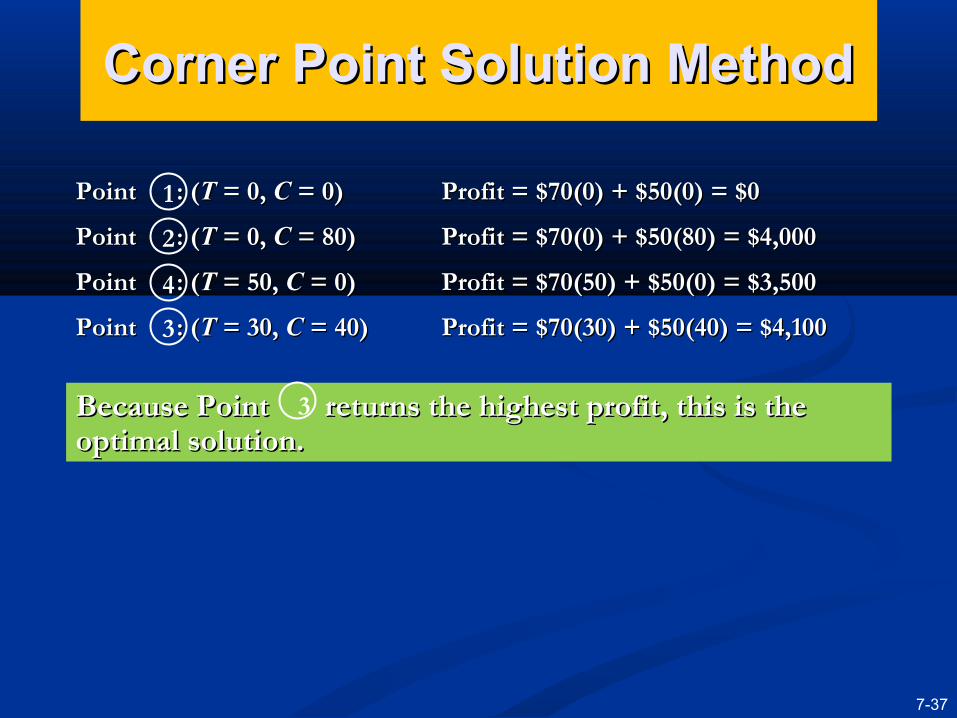
Corner Point Solution MethodCorner Point Solution Method
3
1
2
4
Point : (Point : (TT = 0, = 0, CC = 0) = 0) Profit = $70(0) + $50(0) = $0Profit = $70(0) + $50(0) = $0
Point : (Point : (TT = 0, = 0, CC = 80) = 80) Profit = $70(0) + $50(80) = $4,000Profit = $70(0) + $50(80) = $4,000
Point : (Point : (TT = 50, = 50, CC = 0) = 0) Profit = $70(50) + $50(0) = $3,500Profit = $70(50) + $50(0) = $3,500
Point : (Point : (TT = 30, = 30, CC = 40) = 40) Profit = $70(30) + $50(40) = $4,100Profit = $70(30) + $50(40) = $4,100
Because Point returns the highest profit, this is the Because Point returns the highest profit, this is the optimal solution.optimal solution.
3
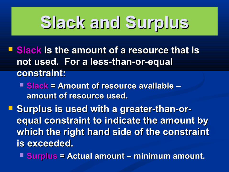
Slack and SurplusSlack and Surplus SlackSlack is the amount of a resource that is is the amount of a resource that is
not used. For a less-than-or-equal not used. For a less-than-or-equal constraint:constraint: SlackSlack = Amount of resource available – = Amount of resource available –
amount of resource used.amount of resource used.
Surplus is used with a greater-than-or-Surplus is used with a greater-than-or-equal constraint to indicate the amount by equal constraint to indicate the amount by which the right hand side of the constraint which the right hand side of the constraint is exceeded.is exceeded. SurplusSurplus = Actual amount – minimum amount. = Actual amount – minimum amount.
Summary of Graphical Summary of Graphical Solution MethodsSolution Methods
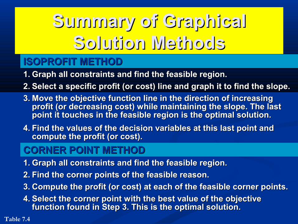
ISOPROFIT METHODISOPROFIT METHOD1.1. Graph all constraints and find the feasible region.Graph all constraints and find the feasible region.
2.2. Select a specific profit (or cost) line and graph it to find the slope.Select a specific profit (or cost) line and graph it to find the slope.
3.3. Move the objective function line in the direction of increasing Move the objective function line in the direction of increasing profit (or decreasing cost) while maintaining the slope. The last profit (or decreasing cost) while maintaining the slope. The last point it touches in the feasible region is the optimal solution.point it touches in the feasible region is the optimal solution.
4.4. Find the values of the decision variables at this last point and Find the values of the decision variables at this last point and compute the profit (or cost).compute the profit (or cost).
CORNER POINT METHODCORNER POINT METHOD1.1. Graph all constraints and find the feasible region.Graph all constraints and find the feasible region.
2.2. Find the corner points of the feasible reason.Find the corner points of the feasible reason.
3.3. Compute the profit (or cost) at each of the feasible corner points.Compute the profit (or cost) at each of the feasible corner points.
4.4. Select the corner point with the best value of the objective Select the corner point with the best value of the objective function found in Step 3. This is the optimal solution.function found in Step 3. This is the optimal solution.
Table 7.4
Copyright ©2012 Pearson Education, Inc. publishing as
Prentice Hall7-40
Solving Flair Furniture’s LP Problem Solving Flair Furniture’s LP Problem Using QM for Windows and ExcelUsing QM for Windows and Excel
Most organizations have access to software Most organizations have access to software to solve big LP problems.to solve big LP problems.
While there are differences between software While there are differences between software implementations, the approach each takes implementations, the approach each takes towards handling LP is basically the same.towards handling LP is basically the same.
Once you are experienced in dealing with Once you are experienced in dealing with computerized LP algorithms, you can easily computerized LP algorithms, you can easily adjust to minor changes.adjust to minor changes.
Using QM for WindowsUsing QM for Windows
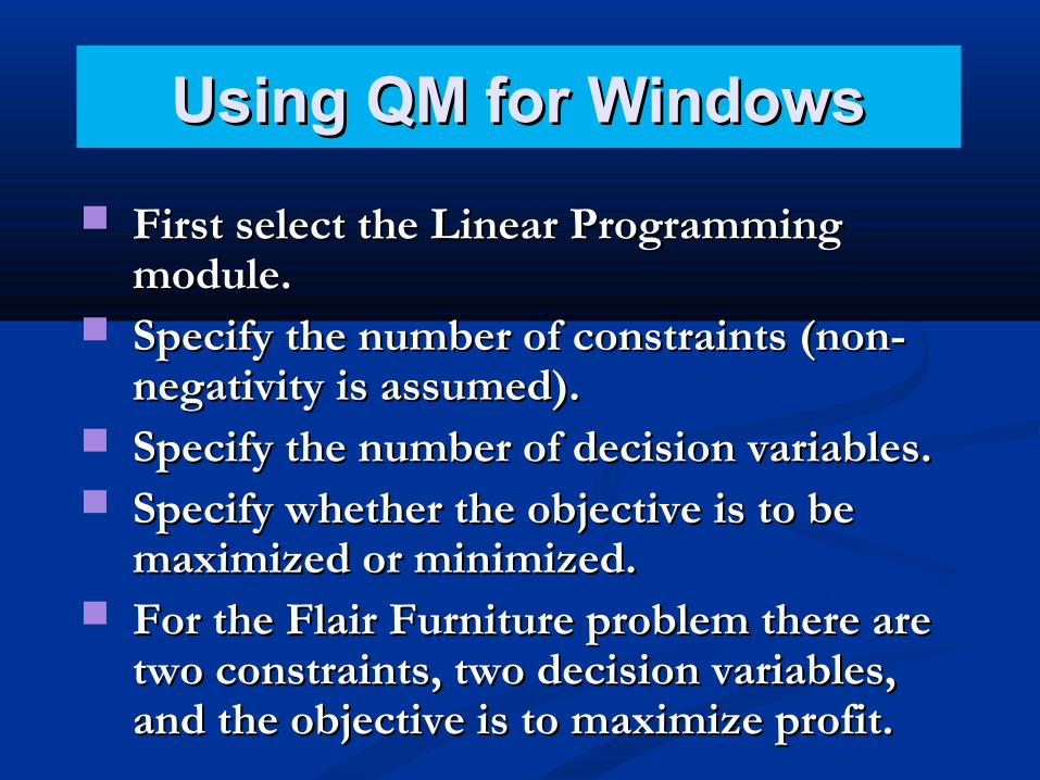
First select the Linear Programming First select the Linear Programming module.module.
Specify the number of constraints (non-Specify the number of constraints (non-negativity is assumed).negativity is assumed).
Specify the number of decision variables.Specify the number of decision variables. Specify whether the objective is to be Specify whether the objective is to be
maximized or minimized.maximized or minimized. For the Flair Furniture problem there are For the Flair Furniture problem there are
two constraints, two decision variables, two constraints, two decision variables, and the objective is to maximize profit.and the objective is to maximize profit.
Using QM for WindowsUsing QM for Windows
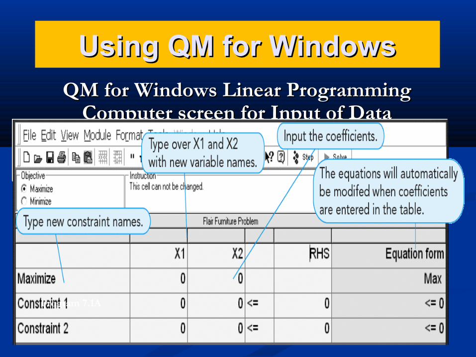
QM for Windows Linear Programming QM for Windows Linear Programming Computer screen for Input of DataComputer screen for Input of Data
Program 7.1A
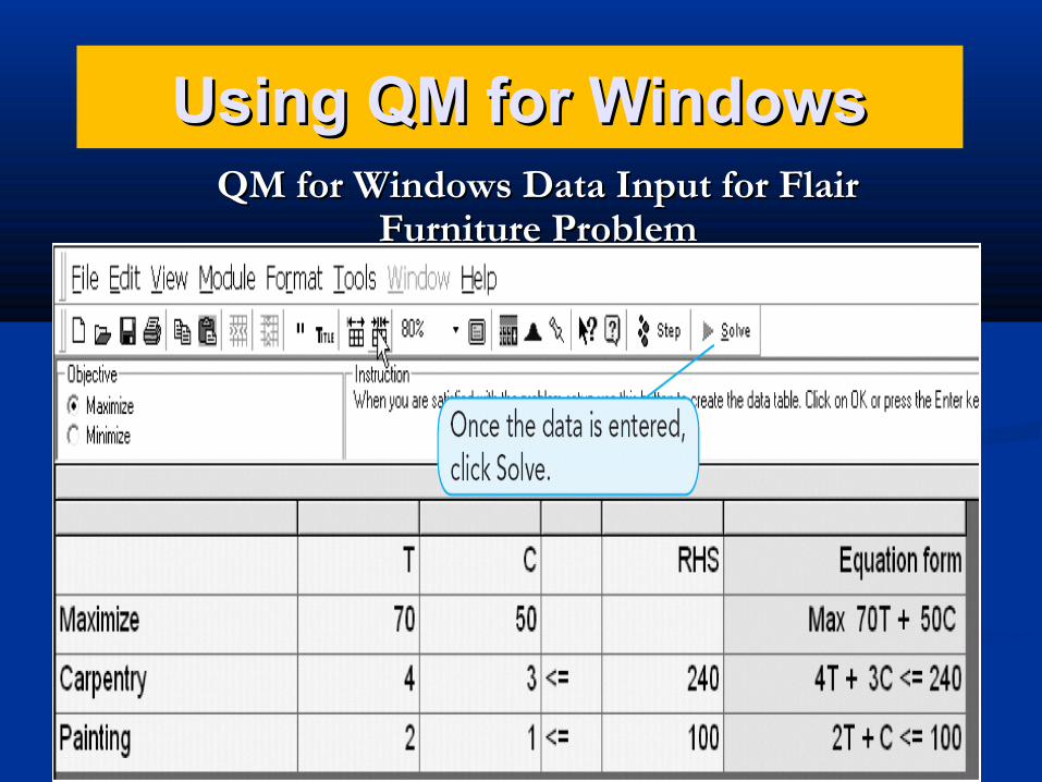
Using QM for WindowsUsing QM for WindowsQM for Windows Data Input for Flair QM for Windows Data Input for Flair
Furniture ProblemFurniture Problem
Program 7.1B
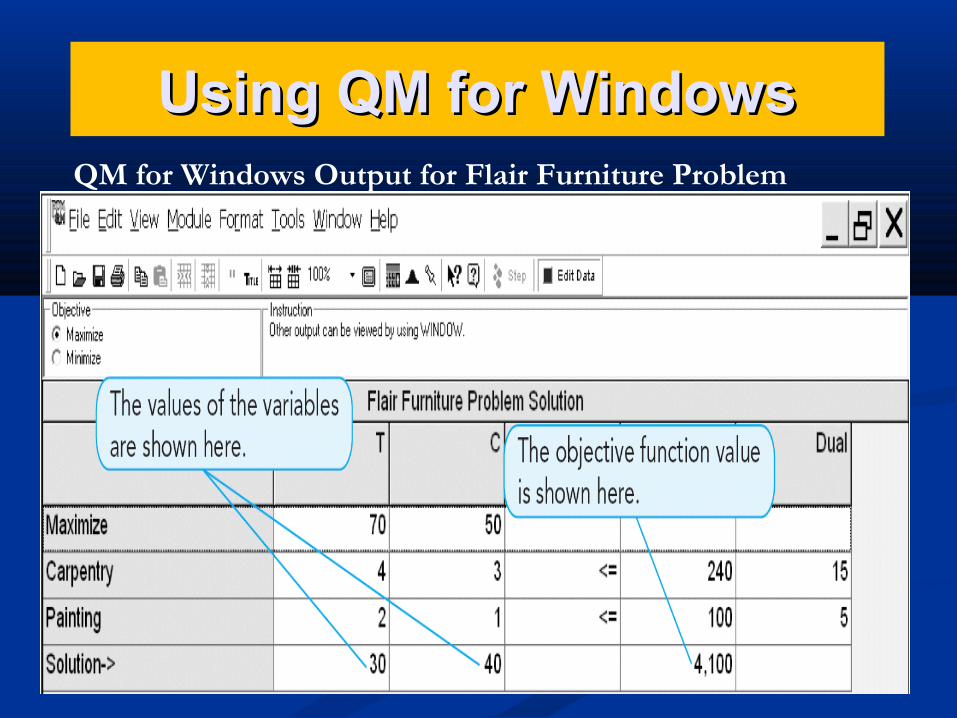
Using QM for WindowsUsing QM for WindowsQM for Windows Output for Flair Furniture Problem
Program 7.1C
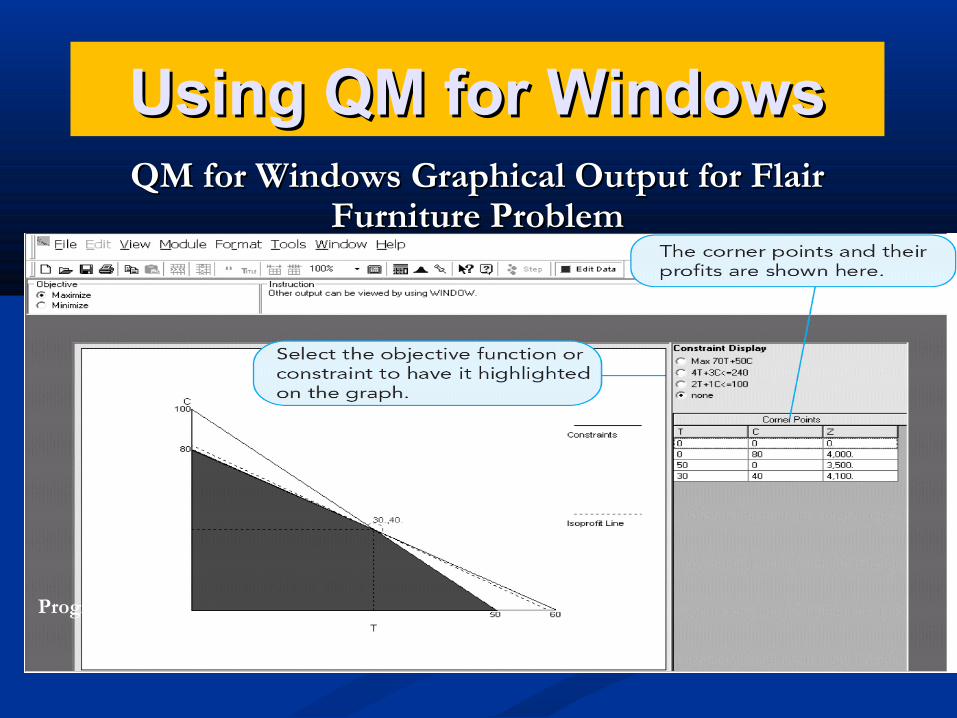
Using QM for WindowsUsing QM for WindowsQM for Windows Graphical Output for Flair QM for Windows Graphical Output for Flair
Furniture ProblemFurniture Problem
Program 7.1D
Using Excel’s Solver Command to Using Excel’s Solver Command to Solve LP ProblemsSolve LP Problems
The Solver tool in Excel can be The Solver tool in Excel can be used to find solutions to:used to find solutions to:LP problems.LP problems.Integer programming problems.Integer programming problems.Noninteger programming Noninteger programming
problems.problems.Solver is limited to 200 variables and Solver is limited to 200 variables and
100 constraints.100 constraints.
Using Solver to Solve the Flair Using Solver to Solve the Flair Furniture ProblemFurniture Problem
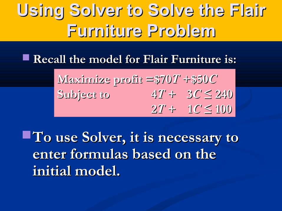
Recall the model for Flair Furniture is:Recall the model for Flair Furniture is:
Maximize profit =Maximize profit =$70$70TT + +$50$50CCSubject toSubject to 44TT + + 33CC ≤ 240≤ 240
22TT + + 11CC ≤ 100≤ 100
To use Solver, it is necessary to To use Solver, it is necessary to enter formulas based on the enter formulas based on the initial model.initial model.
7-48
Using Solver to Solve the Using Solver to Solve the Flair Furniture ProblemFlair Furniture Problem
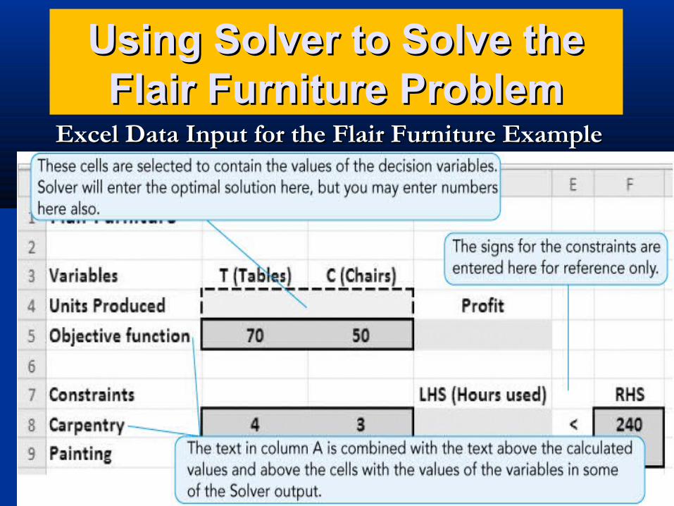
1.1. Enter the variable names, the Enter the variable names, the coefficients for the objective function coefficients for the objective function and constraints, and the right-hand-side and constraints, and the right-hand-side values for each of the constraints.values for each of the constraints.
2.2.Designate specific cells for the values of Designate specific cells for the values of the decision variables.the decision variables.
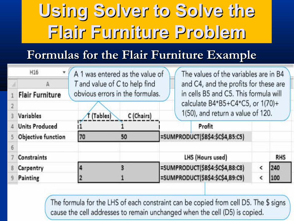
3.3.Write a formula to calculate the value of Write a formula to calculate the value of the objective function.the objective function.
4.4.Write a formula to compute the left-hand Write a formula to compute the left-hand sides of each of the constraints.sides of each of the constraints.
Using Solver to Solve the Using Solver to Solve the Flair Furniture ProblemFlair Furniture Problem
Program 7.2A
Excel Data Input for the Flair Furniture ExampleExcel Data Input for the Flair Furniture Example
Using Solver to Solve the Using Solver to Solve the Flair Furniture ProblemFlair Furniture Problem
Program 7.2B
Formulas for the Flair Furniture ExampleFormulas for the Flair Furniture Example
Using Solver to Solve the Using Solver to Solve the Flair Furniture ProblemFlair Furniture Problem
Program 7.2C
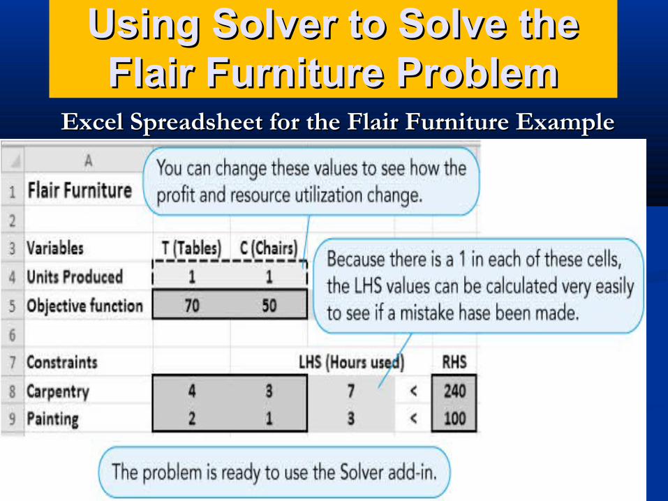
Excel Spreadsheet for the Flair Furniture ExampleExcel Spreadsheet for the Flair Furniture Example
7-52
Using Solver to Solve the Using Solver to Solve the Flair Furniture ProblemFlair Furniture Problem
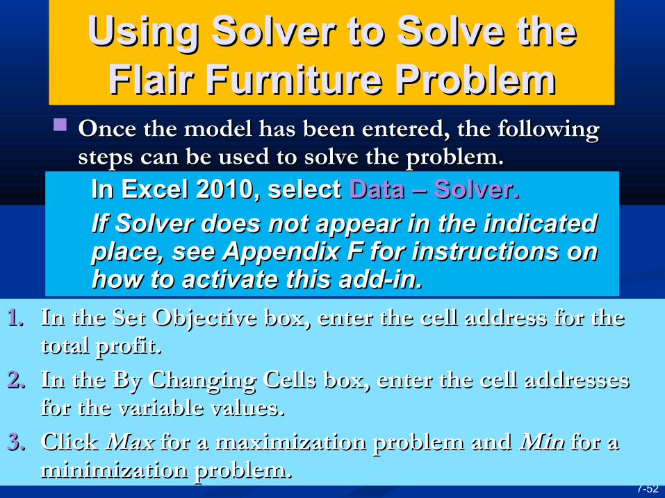
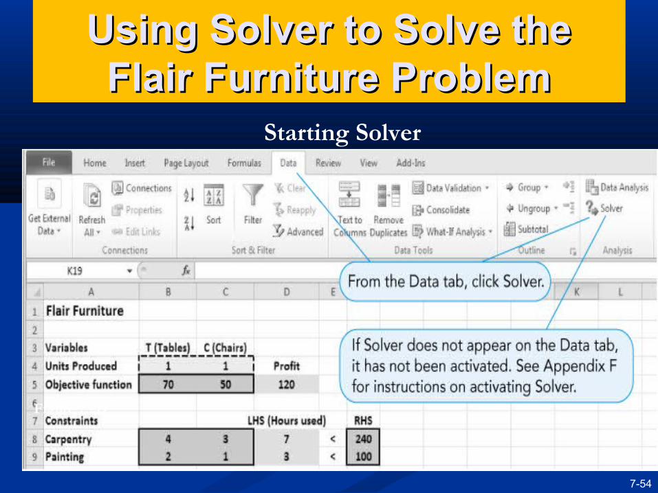
Once the model has been entered, the following Once the model has been entered, the following steps can be used to solve the problem.steps can be used to solve the problem.In Excel 2010, select In Excel 2010, select Data – Solver.Data – Solver.If Solver does not appear in the indicated If Solver does not appear in the indicated place, see Appendix F for instructions on place, see Appendix F for instructions on how to activate this add-in. how to activate this add-in.
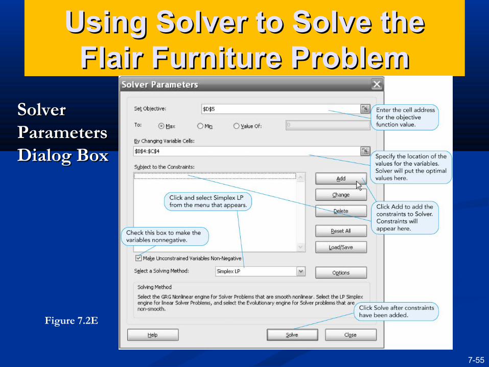
1.1. In the Set Objective box, enter the cell address for the In the Set Objective box, enter the cell address for the total profit.total profit.
2.2. In the By Changing Cells box, enter the cell addresses In the By Changing Cells box, enter the cell addresses for the variable values.for the variable values.
3.3. Click Click MaxMax for a maximization problem and for a maximization problem and MinMin for a for a minimization problem. minimization problem.
7-53
Using Solver to Solve the Flair Using Solver to Solve the Flair Furniture ProblemFurniture Problem
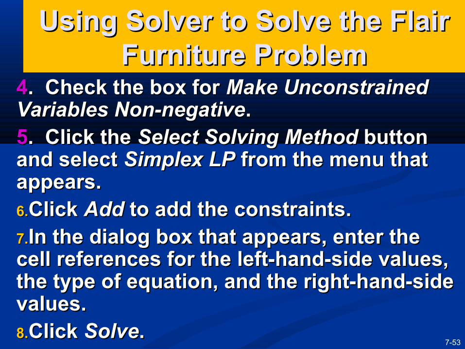
44. Check the box for . Check the box for Make Unconstrained Make Unconstrained Variables Non-negativeVariables Non-negative..55. Click the . Click the Select Solving Method Select Solving Method button button and select and select Simplex LP Simplex LP from the menu that from the menu that appears. appears. 6.6.Click Click AddAdd to add the constraints. to add the constraints.7.7.In the dialog box that appears, enter the In the dialog box that appears, enter the cell references for the left-hand-side values, cell references for the left-hand-side values, the type of equation, and the right-hand-side the type of equation, and the right-hand-side values.values.8.8.Click Click SolveSolve..
7-54
Using Solver to Solve the Using Solver to Solve the Flair Furniture ProblemFlair Furniture Problem
Starting Solver
Figure 7.2D
7-55
Using Solver to Solve the Using Solver to Solve the Flair Furniture ProblemFlair Furniture Problem
Figure 7.2E
Solver Solver Parameters Parameters Dialog BoxDialog Box
7-56
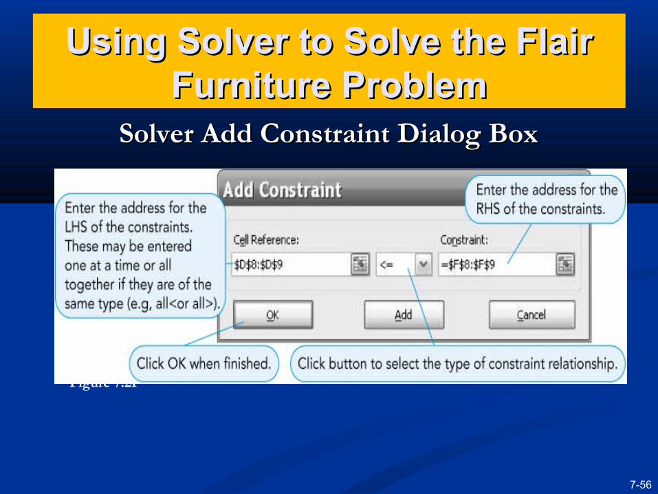
Using Solver to Solve the Flair Using Solver to Solve the Flair Furniture ProblemFurniture Problem
Figure 7.2F
Solver Add Constraint Dialog BoxSolver Add Constraint Dialog Box
7-57
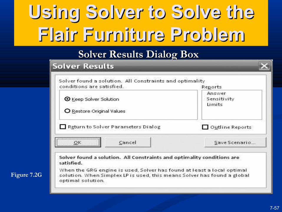
Using Solver to Solve the Using Solver to Solve the Flair Furniture ProblemFlair Furniture Problem
Figure 7.2G
Solver Results Dialog BoxSolver Results Dialog Box
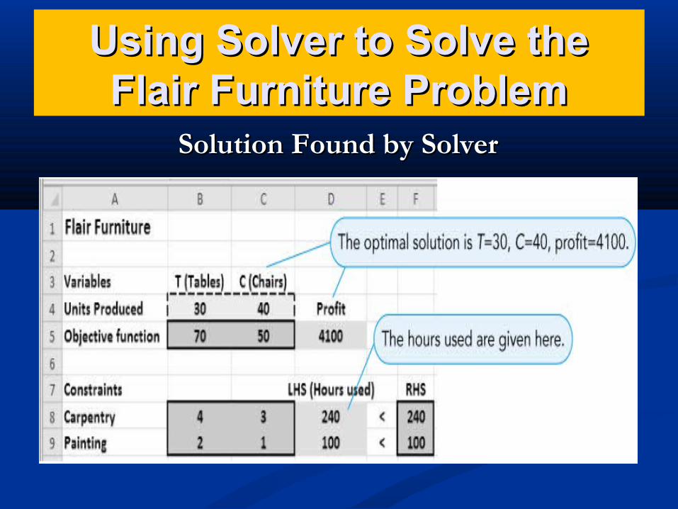
Using Solver to Solve the Using Solver to Solve the Flair Furniture ProblemFlair Furniture Problem
Figure 7.2H
Solution Found by SolverSolution Found by Solver
7-59
Solving Minimization ProblemsSolving Minimization Problems
Many LP problems involve minimizing an Many LP problems involve minimizing an objective such as cost instead of maximizing objective such as cost instead of maximizing a profit function.a profit function.
Minimization problems can be solved Minimization problems can be solved graphically by first setting up the feasible graphically by first setting up the feasible solution region and then using either the solution region and then using either the corner point method or an isocost line corner point method or an isocost line approach (which is analogous to the isoprofit approach (which is analogous to the isoprofit approach in maximization problems) to find approach in maximization problems) to find the values of the decision variables (e.g., the values of the decision variables (e.g., XX11 and and XX22) that yield the minimum cost.) that yield the minimum cost.
7-60
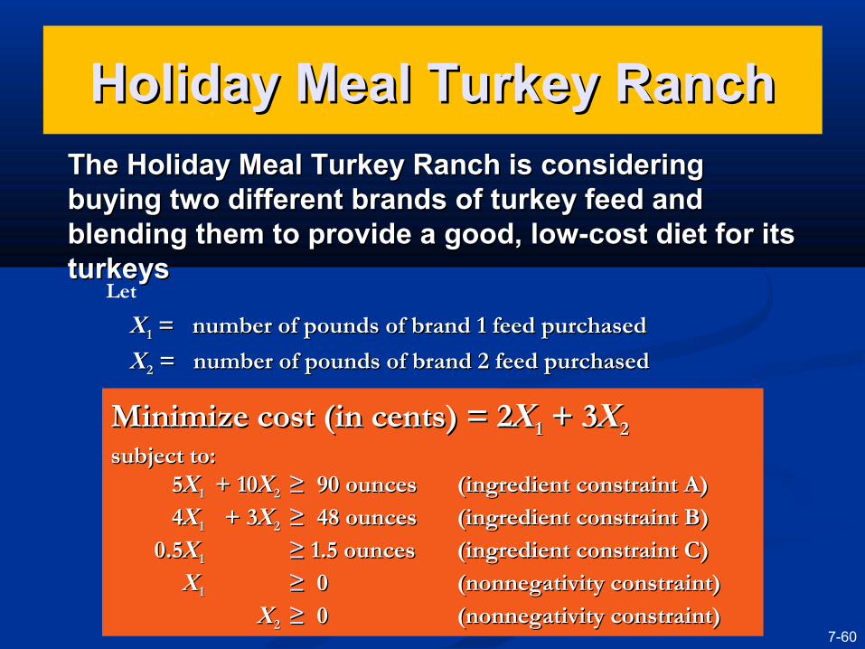
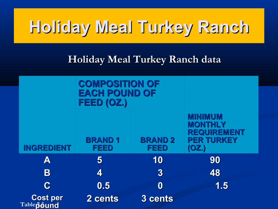
The Holiday Meal Turkey Ranch is considering The Holiday Meal Turkey Ranch is considering buying two different brands of turkey feed and buying two different brands of turkey feed and blending them to provide a good, low-cost diet for its blending them to provide a good, low-cost diet for its turkeys turkeys
Minimize cost (in cents) = 2Minimize cost (in cents) = 2XX11 + 3 + 3XX22
subject to:subject to:55XX11 + 10+ 10XX22 ≥≥ 90 ounces90 ounces (ingredient constraint A)(ingredient constraint A)
44XX11 + 3+ 3XX22 ≥≥ 48 ounces48 ounces (ingredient constraint B)(ingredient constraint B)
0.50.5XX11 ≥≥ 1.5 ounces1.5 ounces (ingredient constraint C)(ingredient constraint C)
XX11 ≥≥ 0 0 (nonnegativity constraint)(nonnegativity constraint)
XX22 ≥≥ 0 0 (nonnegativity constraint)(nonnegativity constraint)
Holiday Meal Turkey RanchHoliday Meal Turkey Ranch
XX11 = number of pounds of brand 1 feed purchased = number of pounds of brand 1 feed purchased
XX22 = number of pounds of brand 2 feed purchased = number of pounds of brand 2 feed purchased
Let
Holiday Meal Turkey RanchHoliday Meal Turkey Ranch
INGREDIENTINGREDIENT
COMPOSITION OF COMPOSITION OF EACH POUND OF EACH POUND OF FEED (OZ.)FEED (OZ.)
MINIMUM MINIMUM MONTHLY MONTHLY REQUIREMENT REQUIREMENT PER TURKEY PER TURKEY (OZ.)(OZ.)
BRAND 1 BRAND 1 FEEDFEED
BRAND 2 BRAND 2 FEEDFEED
AA 55 1010 9090
BB 44 33 4848
CC 0.50.5 00 1.51.5Cost per Cost per poundpound
2 cents2 cents 3 cents3 cents
Holiday Meal Turkey Ranch dataHoliday Meal Turkey Ranch data
Table 7.5
Holiday Meal Turkey RanchHoliday Meal Turkey Ranch
Use the corner point method.Use the corner point method. First construct the feasible First construct the feasible
solution region.solution region. The optimal solution will lie at The optimal solution will lie at
one of the corners as it would one of the corners as it would in a maximization problem.in a maximization problem.
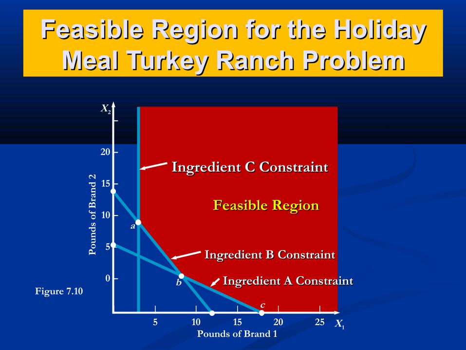
Feasible Region for the Holiday Feasible Region for the Holiday Meal Turkey Ranch ProblemMeal Turkey Ranch Problem
–
20 –
15 –
10 –
5 –
0 –
X2
| | | | | |
5 10 15 20 25 X1
Pou
nds
of B
rand
2
Pounds of Brand 1
Ingredient C ConstraintIngredient C Constraint
Ingredient B ConstraintIngredient B Constraint
Ingredient A ConstraintIngredient A Constraint
Feasible RegionFeasible Regiona
b
cFigure 7.10
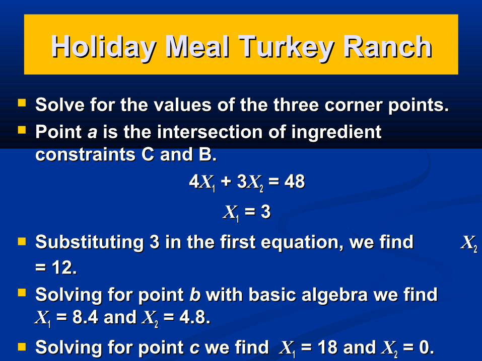
Holiday Meal Turkey RanchHoliday Meal Turkey Ranch
Solve for the values of the three corner points.Solve for the values of the three corner points. Point Point aa is the intersection of ingredient is the intersection of ingredient
constraints C and B.constraints C and B.
44XX11 + 3 + 3XX22 = 48 = 48
XX11 = 3 = 3
Substituting 3 in the first equation, we find Substituting 3 in the first equation, we find XX22
= 12.= 12. Solving for point Solving for point bb with basic algebra we find with basic algebra we find XX11 = 8.4 and = 8.4 and XX22 = 4.8. = 4.8.
Solving for point Solving for point cc we find we find XX11 = 18 and = 18 and XX22 = 0. = 0.
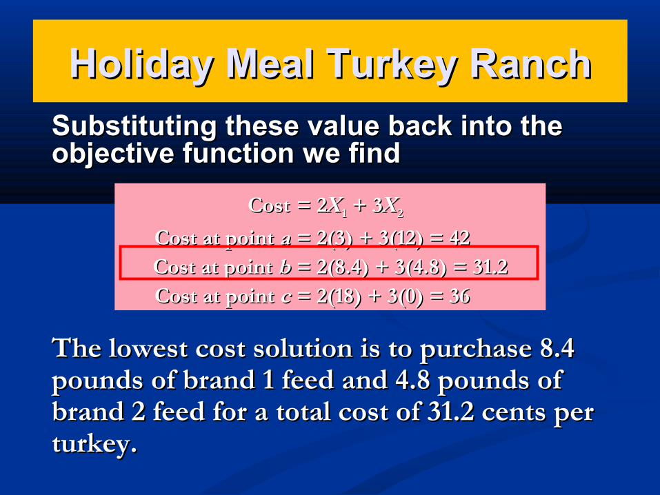
Substituting these value back into the Substituting these value back into the objective function we findobjective function we find
CostCost = 2= 2XX11 + 3 + 3XX22
Cost at point Cost at point aa = 2(3) + 3(12) = 42= 2(3) + 3(12) = 42Cost at point Cost at point bb = 2(8.4) + 3(4.8) = 31.2= 2(8.4) + 3(4.8) = 31.2Cost at point Cost at point cc = 2(18) + 3(0) = 36= 2(18) + 3(0) = 36
Holiday Meal Turkey RanchHoliday Meal Turkey Ranch
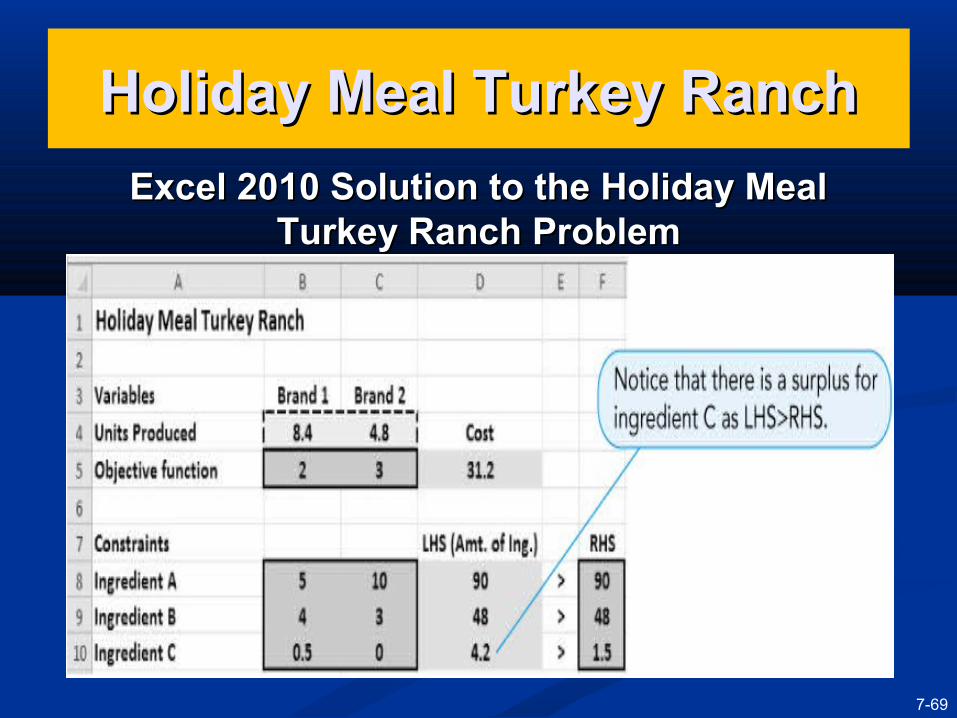
The lowest cost solution is to purchase 8.4 The lowest cost solution is to purchase 8.4 pounds of brand 1 feed and 4.8 pounds of pounds of brand 1 feed and 4.8 pounds of brand 2 feed for a total cost of 31.2 cents per brand 2 feed for a total cost of 31.2 cents per turkey.turkey.
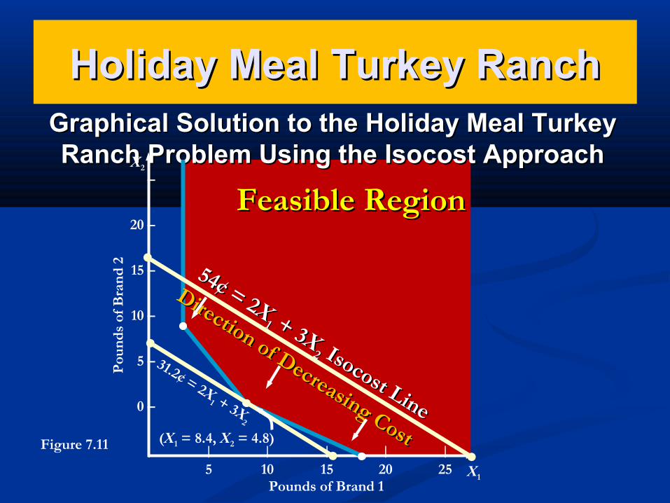
Graphical Solution to the Holiday Meal Turkey Graphical Solution to the Holiday Meal Turkey Ranch Problem Using the Isocost ApproachRanch Problem Using the Isocost Approach
Holiday Meal Turkey RanchHoliday Meal Turkey Ranch
–
20 –
15 –
10 –
5 –
0 –
X2
| | | | | |
5 10 15 20 25 X1
Pou
nds
of B
rand
2
Pounds of Brand 1
Figure 7.11
Feasible RegionFeasible Region
5454¢ = 2¢ = 2XX
11 + 3 + 3XX
22 Isocost Line
Isocost Line
Direction of Decreasing Cost
Direction of Decreasing Cost
31.2¢ = 2X1 + 3X
2
(X1 = 8.4, X2 = 4.8)
7-67
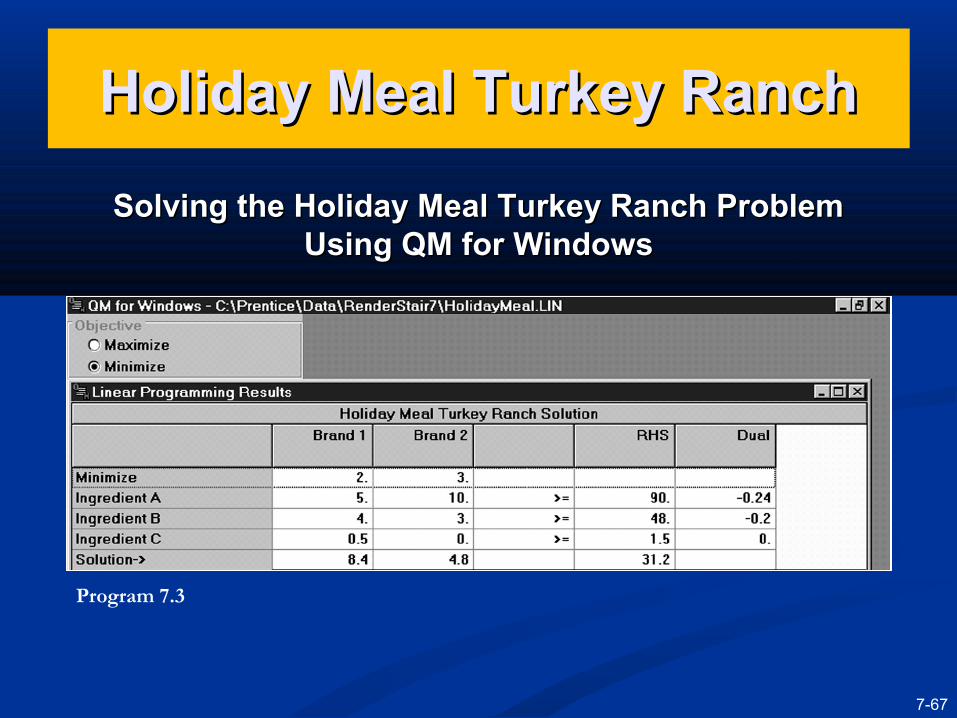
Solving the Holiday Meal Turkey Ranch Problem Solving the Holiday Meal Turkey Ranch Problem Using QM for WindowsUsing QM for Windows
Holiday Meal Turkey RanchHoliday Meal Turkey Ranch
Program 7.3
Holiday Meal Turkey RanchHoliday Meal Turkey Ranch
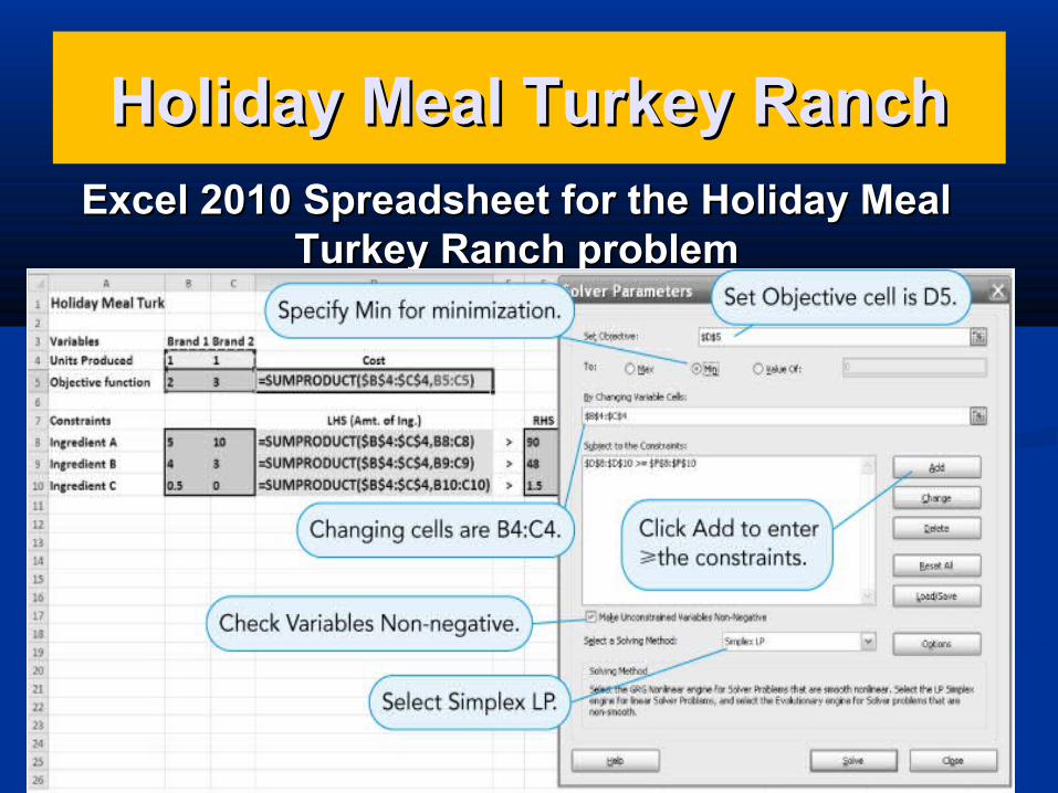
Program 7.4A
Excel 2010 Spreadsheet for the Holiday Meal Excel 2010 Spreadsheet for the Holiday Meal Turkey Ranch problemTurkey Ranch problem
7-69
Holiday Meal Turkey RanchHoliday Meal Turkey Ranch
Program 7.4B
Excel 2010 Solution to the Holiday Meal Excel 2010 Solution to the Holiday Meal Turkey Ranch ProblemTurkey Ranch Problem
7-70
Four Special Cases in LPFour Special Cases in LP
Four special cases and difficulties Four special cases and difficulties arise at times when using the arise at times when using the graphical approach to solving LP graphical approach to solving LP problems.problems. No feasible solutionNo feasible solution UnboundednessUnboundedness RedundancyRedundancy Alternate Optimal SolutionsAlternate Optimal Solutions
7-71
Four Special Cases in LPFour Special Cases in LP
No feasible solutionNo feasible solution This exists when there is no solution to This exists when there is no solution to
the problem that satisfies all the the problem that satisfies all the constraint equations.constraint equations.
No feasible solution region exists.No feasible solution region exists. This is a common occurrence in the real This is a common occurrence in the real
world.world. Generally one or more constraints are Generally one or more constraints are
relaxed until a solution is found.relaxed until a solution is found.
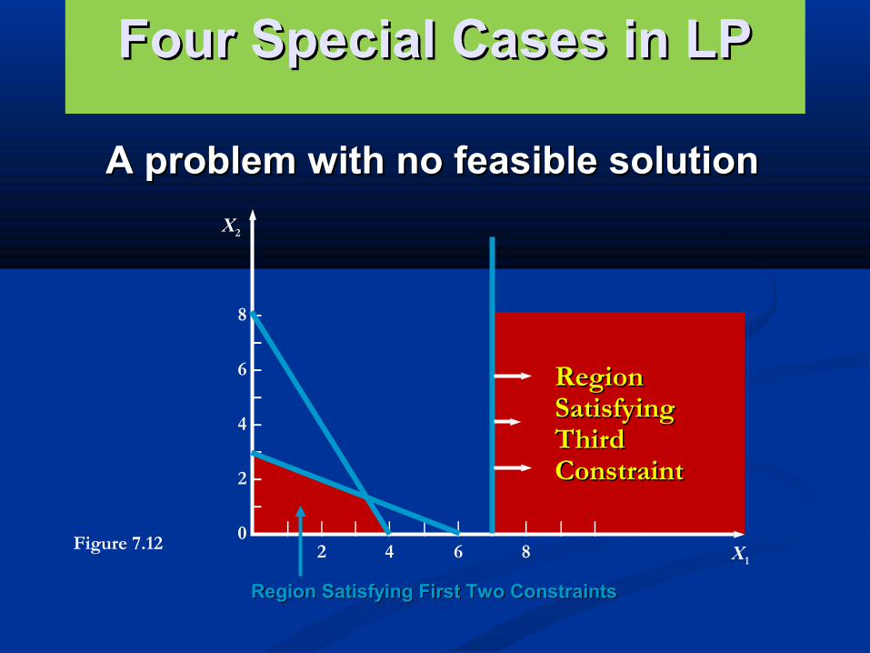
Four Special Cases in LPFour Special Cases in LP
A problem with no feasible solutionA problem with no feasible solution
8 –
–
6 –
–
4 –
–
2 –
–
0 –
X2
| | | | | | | | | |
2 4 6 8 X1
Region Satisfying First Two ConstraintsRegion Satisfying First Two Constraints
Figure 7.12
Region Region Satisfying Satisfying Third Third ConstraintConstraint
7-73
Four Special Cases in LPFour Special Cases in LP
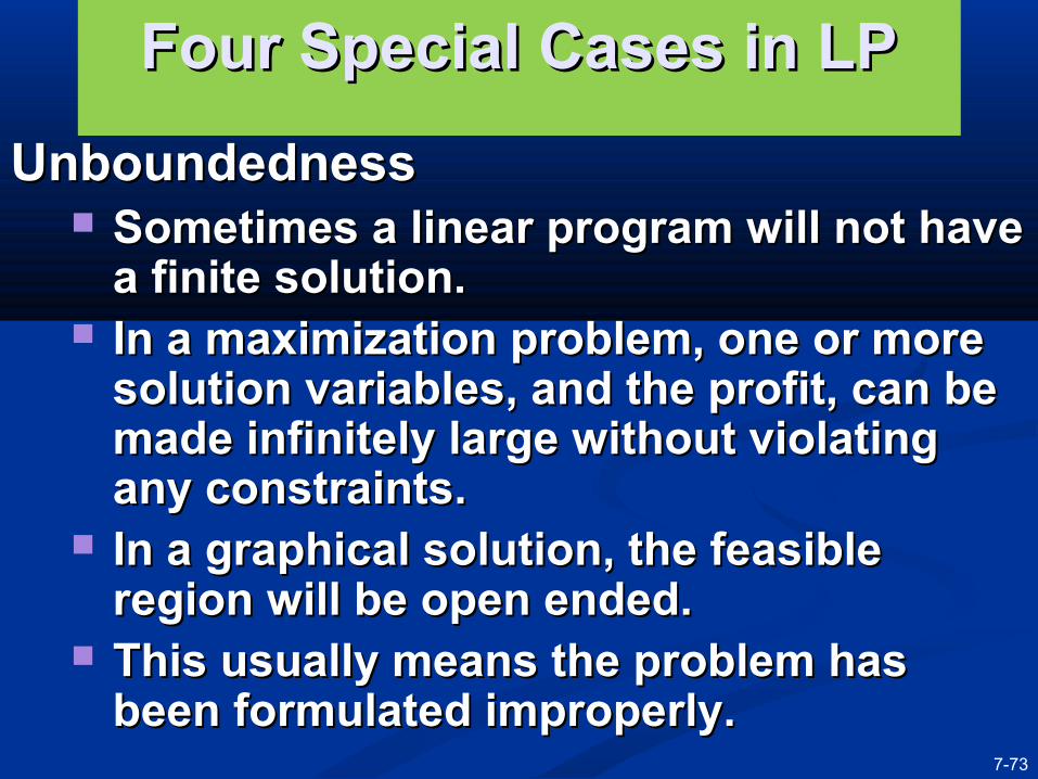
UnboundednessUnboundedness Sometimes a linear program will not have Sometimes a linear program will not have
a finite solution.a finite solution. In a maximization problem, one or more In a maximization problem, one or more
solution variables, and the profit, can be solution variables, and the profit, can be made infinitely large without violating made infinitely large without violating any constraints.any constraints.
In a graphical solution, the feasible In a graphical solution, the feasible region will be open ended.region will be open ended.
This usually means the problem has This usually means the problem has been formulated improperly.been formulated improperly.
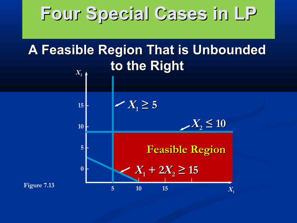
Four Special Cases in LPFour Special Cases in LP
A Feasible Region That is Unbounded A Feasible Region That is Unbounded to the Rightto the Right
15 –
10 –
5 –
0 –
X2
| | | | |
5 10 15 X1
Figure 7.13
Feasible RegionFeasible Region
XX11 ≥ 5≥ 5
XX22 ≤ 10≤ 10
XX11 + 2 + 2XX22 ≥ 15≥ 15
Four Special Cases in LPFour Special Cases in LP
RedundancyRedundancy A redundant constraint is one that does A redundant constraint is one that does
not affect the feasible solution region.not affect the feasible solution region. One or more constraints may be binding.One or more constraints may be binding. This is a very common occurrence in the This is a very common occurrence in the
real world.real world. It causes no particular problems, but It causes no particular problems, but
eliminating redundant constraints eliminating redundant constraints simplifies the model.simplifies the model.
7-76
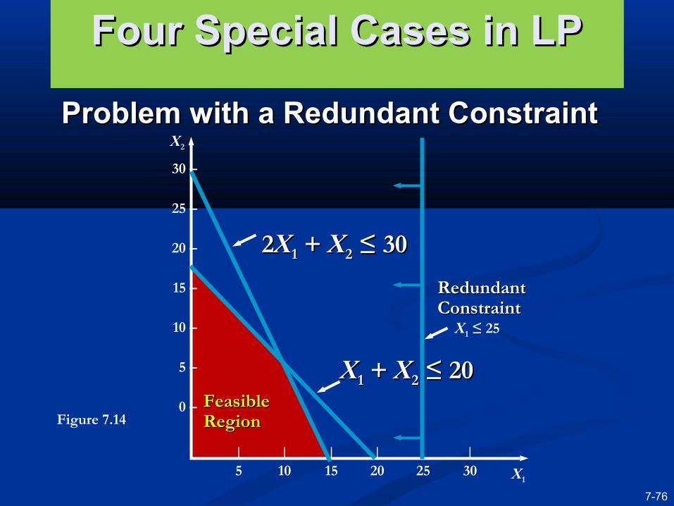
Four Special Cases in LPFour Special Cases in LP
Problem with a Redundant ConstraintProblem with a Redundant Constraint
30 –
25 –
20 –
15 –
10 –
5 –
0 –
X2
| | | | | |
5 10 15 20 25 30 X1
Figure 7.14
Redundant Redundant ConstraintConstraint
Feasible Feasible RegionRegion
X1 ≤ 25
22XX11 + + XX22 ≤ 30≤ 30
XX11 + + XX22 ≤ 20≤ 20
Four Special Cases in LPFour Special Cases in LP
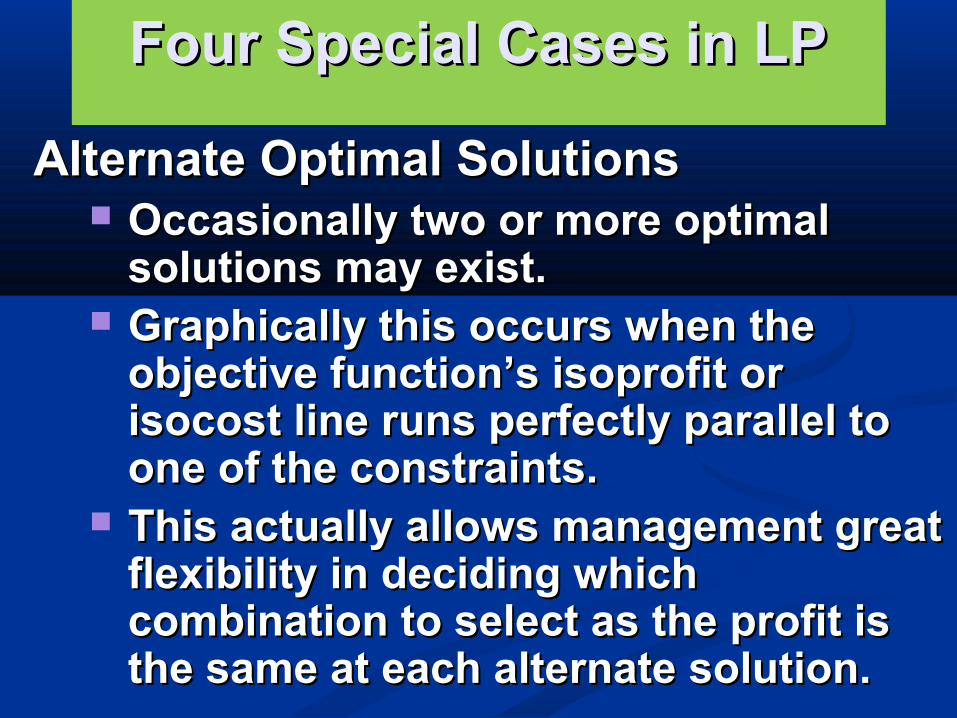
Alternate Optimal SolutionsAlternate Optimal Solutions Occasionally two or more optimal Occasionally two or more optimal
solutions may exist.solutions may exist. Graphically this occurs when the Graphically this occurs when the
objective function’s isoprofit or objective function’s isoprofit or isocost line runs perfectly parallel to isocost line runs perfectly parallel to one of the constraints.one of the constraints.
This actually allows management great This actually allows management great flexibility in deciding which flexibility in deciding which combination to select as the profit is combination to select as the profit is the same at each alternate solution.the same at each alternate solution.
7-78
Four Special Cases in LPFour Special Cases in LP
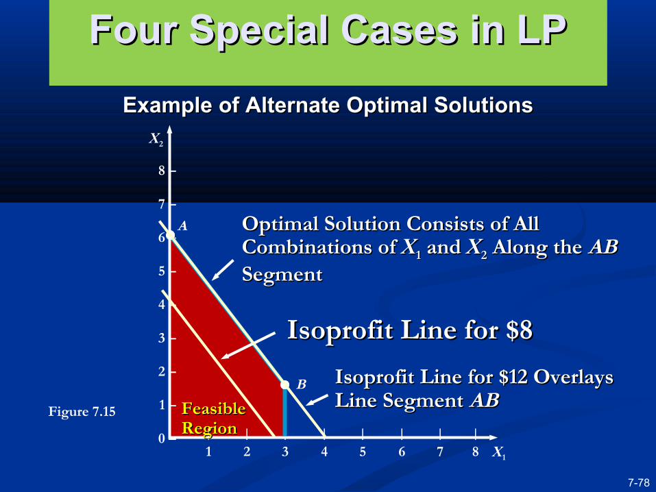
Example of Alternate Optimal SolutionsExample of Alternate Optimal Solutions
8 –
7 –
6 –
5 –
4 –
3 –
2 –
1 –
0 –
X2
| | | | | | | |
1 2 3 4 5 6 7 8 X1
Figure 7.15 Feasible Feasible RegionRegion
Isoprofit Line for $8Isoprofit Line for $8
Optimal Solution Consists of All Optimal Solution Consists of All Combinations of Combinations of XX11 and and XX22 Along the Along the AB AB SegmentSegment
Isoprofit Line for $12 Overlays Isoprofit Line for $12 Overlays Line Segment Line Segment ABAB
B
A
7-79
Sensitivity AnalysisSensitivity Analysis
Optimal solutions to LP problems thus far have Optimal solutions to LP problems thus far have been found under what are called been found under what are called deterministic deterministic assumptions.assumptions.
This means that we assume complete certainty This means that we assume complete certainty in the data and relationships of a problem.in the data and relationships of a problem.
But in the real world, conditions are dynamic But in the real world, conditions are dynamic and changing.and changing.
We can analyze how We can analyze how sensitivesensitive a deterministic a deterministic solution is to changes in the assumptions of the solution is to changes in the assumptions of the model.model.
This is called This is called sensitivity analysissensitivity analysis, , postoptimality postoptimality analysisanalysis, , parametric programmingparametric programming, or , or optimality optimality analysis.analysis.
7-80
Sensitivity AnalysisSensitivity Analysis
Sensitivity analysis often involves a series of Sensitivity analysis often involves a series of what-if? questions concerning constraints, what-if? questions concerning constraints, variable coefficients, and the objective function.variable coefficients, and the objective function.
One way to do this is the trial-and-error method One way to do this is the trial-and-error method where values are changed and the entire model where values are changed and the entire model is resolved.is resolved.
The preferred way is to use an analytic post-The preferred way is to use an analytic post-optimality analysis.optimality analysis.
After a problem has been solved, we determine a After a problem has been solved, we determine a range of changes in problem parameters that will range of changes in problem parameters that will not affect the optimal solution or change the not affect the optimal solution or change the variables in the solution.variables in the solution.
7-81
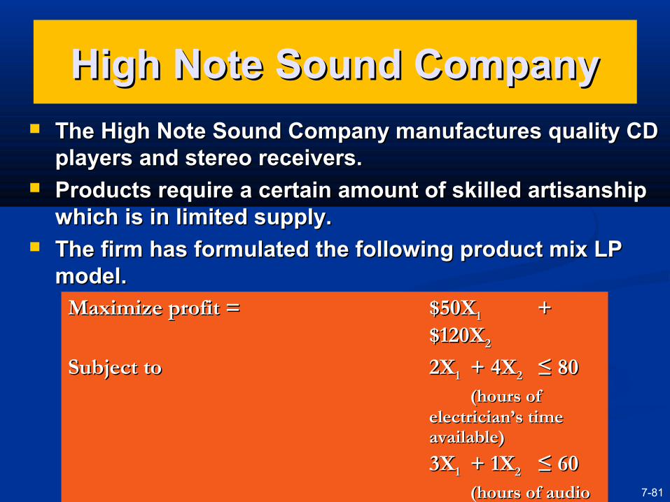
The High Note Sound Company manufactures quality CD The High Note Sound Company manufactures quality CD players and stereo receivers.players and stereo receivers.
Products require a certain amount of skilled artisanship Products require a certain amount of skilled artisanship which is in limited supply.which is in limited supply.
The firm has formulated the following product mix LP The firm has formulated the following product mix LP model.model.
High Note Sound CompanyHigh Note Sound Company
Maximize profit =Maximize profit = $50X$50X11 + + $120X$120X22
Subject toSubject to 2X2X11 + 4X+ 4X22 ≤ 80≤ 80(hours of (hours of
electrician’s time electrician’s time available)available)
3X3X11 + 1X+ 1X22 ≤ 60≤ 60(hours of audio (hours of audio
technician’s time technician’s time available)available)
XX11, X, X22 ≥ 0≥ 0
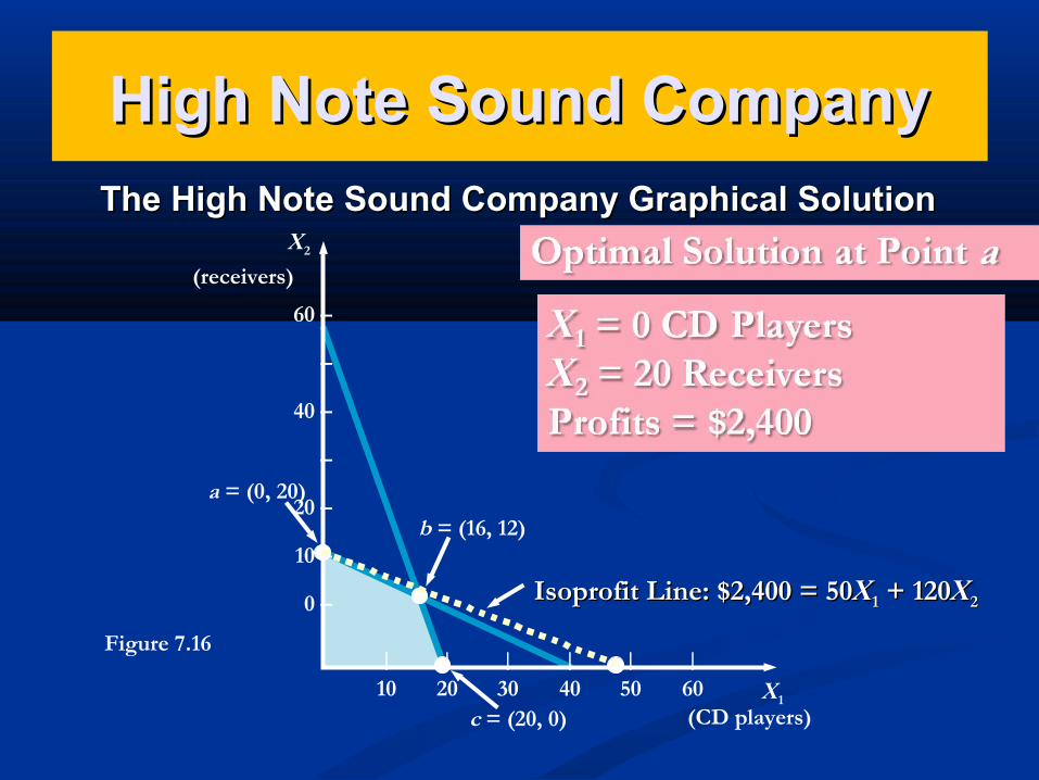
The High Note Sound Company Graphical SolutionThe High Note Sound Company Graphical Solution
High Note Sound CompanyHigh Note Sound Company
b = (16, 12)
a = (0, 20)
Isoprofit Line: $2,400 = 50Isoprofit Line: $2,400 = 50XX11 + 120 + 120XX22
60 –
–
40 –
–
20 –
10 –
0 –
X2
| | | | | |
10 20 30 40 50 60 X1
(receivers)
(CD players)c = (20, 0)
Figure 7.16
7-83
Changes in the Changes in the Objective Function CoefficientObjective Function Coefficient
In real-life problems, contribution rates in the In real-life problems, contribution rates in the objective functions fluctuate periodically.objective functions fluctuate periodically.
Graphically, this means that although the feasible Graphically, this means that although the feasible solution region remains exactly the same, the solution region remains exactly the same, the slope of the isoprofit or isocost line will change.slope of the isoprofit or isocost line will change.
We can often make modest increases or We can often make modest increases or decreases in the objective function coefficient of decreases in the objective function coefficient of any variable without changing the current optimal any variable without changing the current optimal corner point.corner point.
We need to know how much an objective function We need to know how much an objective function coefficient can change before the optimal solution coefficient can change before the optimal solution would be at a different corner point.would be at a different corner point.
7-84
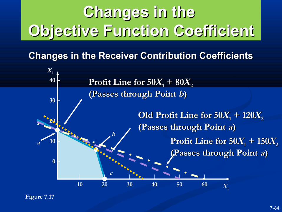
Changes in the Changes in the Objective Function CoefficientObjective Function Coefficient
Changes in the Receiver Contribution CoefficientsChanges in the Receiver Contribution Coefficients
ba
Profit Line for 50Profit Line for 50XX11 + 80 + 80XX22
(Passes through Point (Passes through Point bb))
40 –
30 –
20 –
10 –
0 –
X2
| | | | | |
10 20 30 40 50 60 X1
c
Figure 7.17
Old Profit Line for 50Old Profit Line for 50XX11 + 120 + 120XX22
(Passes through Point (Passes through Point aa))
Profit Line for 50Profit Line for 50XX11 + 150 + 150XX22
(Passes through Point (Passes through Point aa))
7-85
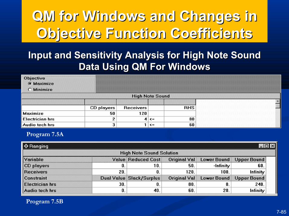
QM for Windows and Changes in QM for Windows and Changes in Objective Function CoefficientsObjective Function Coefficients
Input and Sensitivity Analysis for High Note Sound Input and Sensitivity Analysis for High Note Sound Data Using QM For WindowsData Using QM For Windows
Program 7.5B
Program 7.5A
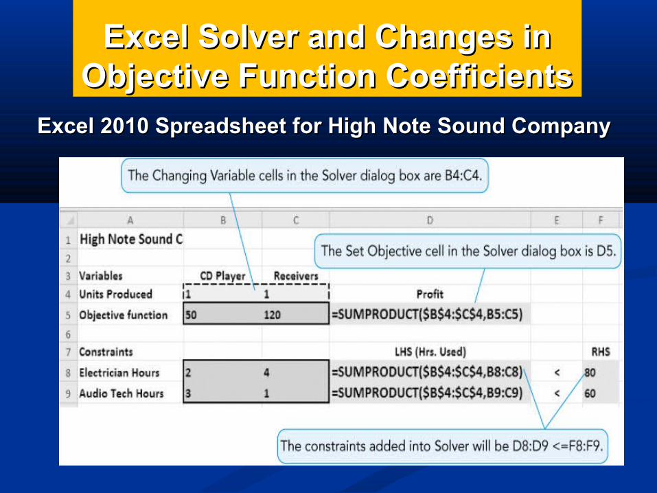
Excel Solver and Changes in Excel Solver and Changes in Objective Function CoefficientsObjective Function Coefficients
Excel 2010 Spreadsheet for High Note Sound CompanyExcel 2010 Spreadsheet for High Note Sound Company
Program 7.6A
7-87
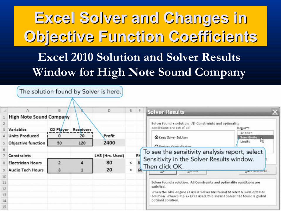
Excel Solver and Changes in Excel Solver and Changes in Objective Function CoefficientsObjective Function Coefficients
Excel 2010 Solution and Solver Results Window for High Note Sound Company
Figure 7.6B
7-88
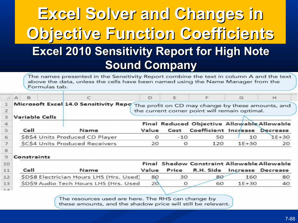
Excel Solver and Changes in Excel Solver and Changes in Objective Function CoefficientsObjective Function CoefficientsExcel 2010 Sensitivity Report for High Note Excel 2010 Sensitivity Report for High Note
Sound CompanySound Company
Program 7.6C
7-89
Changes in the Changes in the Technological CoefficientsTechnological Coefficients
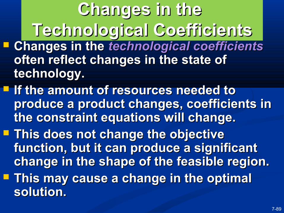
Changes in the Changes in the technological coefficientstechnological coefficients often reflect changes in the state of often reflect changes in the state of technology.technology.
If the amount of resources needed to If the amount of resources needed to produce a product changes, coefficients in produce a product changes, coefficients in the constraint equations will change.the constraint equations will change.
This does not change the objective This does not change the objective function, but it can produce a significant function, but it can produce a significant change in the shape of the feasible region.change in the shape of the feasible region.
This may cause a change in the optimal This may cause a change in the optimal solution. solution.
7-90
Changes in the Changes in the Technological CoefficientsTechnological Coefficients
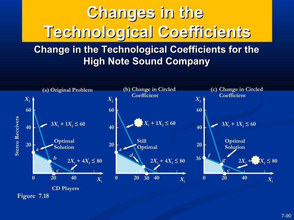
Change in the Technological Coefficients for the Change in the Technological Coefficients for the High Note Sound CompanyHigh Note Sound Company
(a) Original Problem
3X1 + 1X2 ≤ 60
2X1 + 4X2 ≤ 80
Optimal Solution
X2
60 –
40 –
20 –
–
| | |
0 20 40 X1
Ster
eo R
ecei
vers
CD Players
(b) Change in Circled Coefficient
2 X1 + 1X2 ≤ 60
2X1 + 4X2 ≤ 80
Still Optimal
3X1 + 1X2 ≤ 60
2X1 + 5 X2 ≤ 80
Optimal Solutiona
d
e
60 –
40 –
20 –
–
| | |
0 20 40
X2
X1
16
60 –
40 –
20 –
–
| | |
0 20 40
X2
X1
|
30
(c) Change in Circled Coefficient
a
b
c
fg
c
Figure 7.18
7-91
Changes in Resources or Changes in Resources or Right-Hand-Side ValuesRight-Hand-Side Values
The right-hand-side values of the The right-hand-side values of the constraints often represent resources constraints often represent resources available to the firm.available to the firm.
If additional resources were available, a If additional resources were available, a higher total profit could be realized.higher total profit could be realized.
Sensitivity analysis about resources will Sensitivity analysis about resources will help answer questions about how much help answer questions about how much should be paid for additional resources should be paid for additional resources and how much more of a resource would and how much more of a resource would be useful.be useful.
Changes in Resources or Right-Changes in Resources or Right-Hand-Side ValuesHand-Side Values
If the right-hand side of a constraint is changed, If the right-hand side of a constraint is changed, the feasible region will change (unless the the feasible region will change (unless the constraint is redundant).constraint is redundant).
Often the optimal solution will change.Often the optimal solution will change. The amount of change in the objective function The amount of change in the objective function
value that results from a unit change in one of the value that results from a unit change in one of the resources available is called the resources available is called the dual pricedual price or or dual dual valuevalue . .
The dual price for a constraint is the improvement The dual price for a constraint is the improvement in the objective function value that results from a in the objective function value that results from a one-unit increase in the right-hand side of the one-unit increase in the right-hand side of the constraint.constraint.
7-93
Changes in Resources or Changes in Resources or Right-Hand-Side ValuesRight-Hand-Side Values
However, the amount of possible increase in However, the amount of possible increase in the right-hand side of a resource is limited.the right-hand side of a resource is limited.
If the number of hours increased beyond the If the number of hours increased beyond the upper bound, then the objective function upper bound, then the objective function would no longer increase by the dual price.would no longer increase by the dual price.
There would simply be excess (There would simply be excess (slackslack) hours ) hours of a resource or the objective function may of a resource or the objective function may change by an amount different from the dual change by an amount different from the dual price.price.
The dual price is relevant only within limits.The dual price is relevant only within limits.
7-94
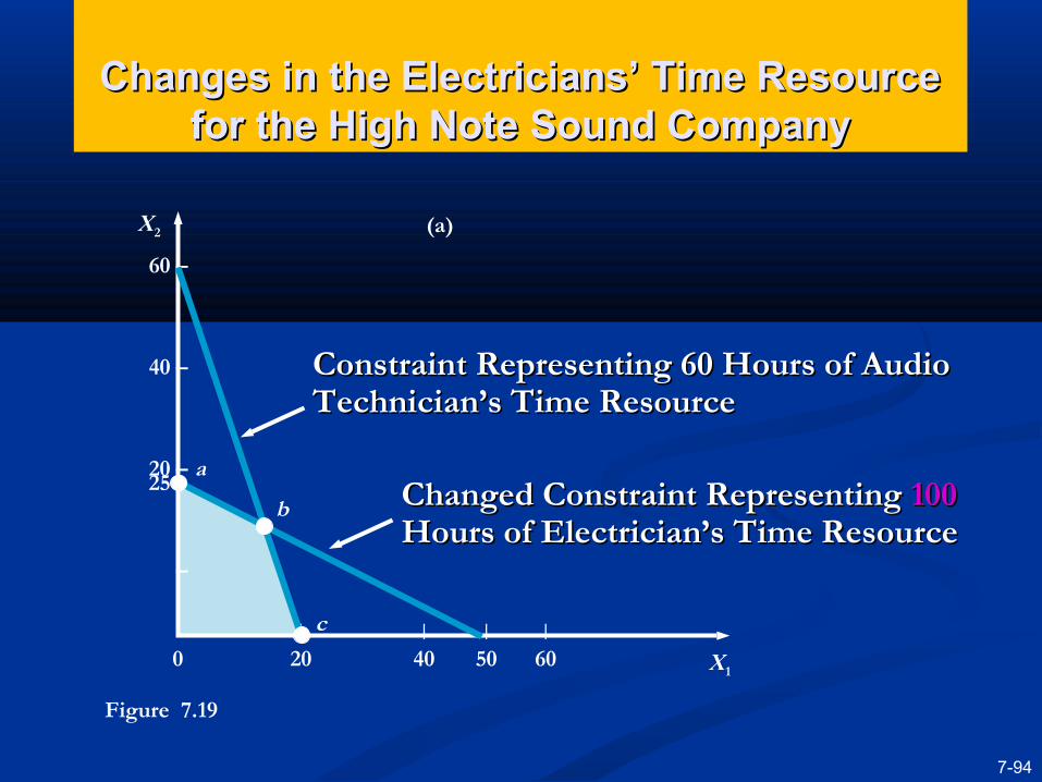
Changes in the Electricians’ Time Resource Changes in the Electricians’ Time Resource for the High Note Sound Companyfor the High Note Sound Company
60 –
40 –
20 –
–
25 –
| | |
0 20 40 60|
50 X1
X2 (a)
a
b
c
Constraint Representing 60 Hours of Audio Constraint Representing 60 Hours of Audio Technician’s Time ResourceTechnician’s Time Resource
Changed Constraint Representing Changed Constraint Representing 100100 Hours of Electrician’s Time ResourceHours of Electrician’s Time Resource
Figure 7.19
7-95
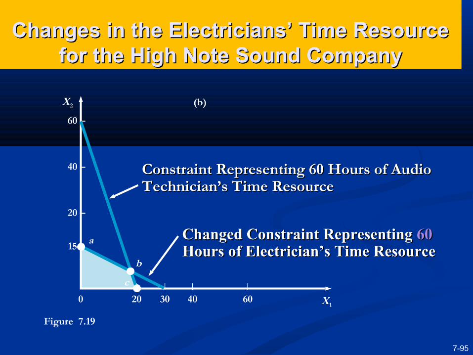
Changes in the Electricians’ Time Resource Changes in the Electricians’ Time Resource for the High Note Sound Companyfor the High Note Sound Company
60 –
40 –
20 –
–15 –
| | |
0 20 40 60|
30 X1
X2 (b)
a
b
c
Constraint Representing 60 Hours of Audio Constraint Representing 60 Hours of Audio Technician’s Time ResourceTechnician’s Time Resource
Changed Constraint Representing Changed Constraint Representing 6060 Hours of Electrician’s Time ResourceHours of Electrician’s Time Resource
Figure 7.19
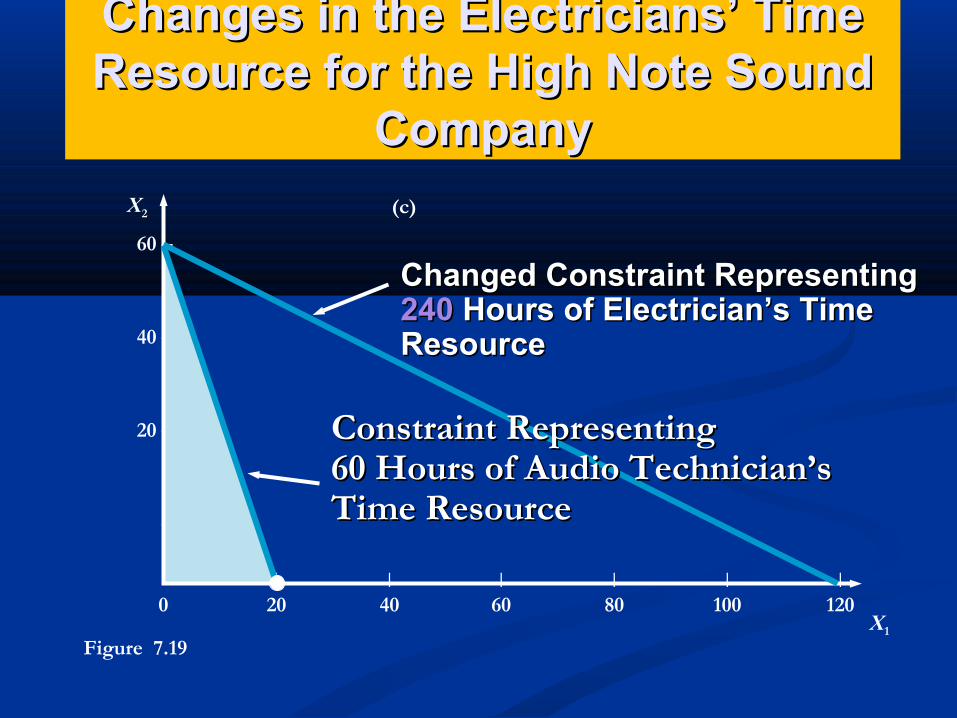
Changes in the Electricians’ Time Changes in the Electricians’ Time Resource for the High Note Sound Resource for the High Note Sound
CompanyCompany
60 –
40 –
20 –
–
| | | | | |
0 20 40 60 80 100 120X1
X2 (c)
Constraint Representing Constraint Representing 60 Hours of Audio Technician’s 60 Hours of Audio Technician’s Time ResourceTime Resource
Changed Constraint Representing Changed Constraint Representing 240240 Hours of Electrician’s Time Hours of Electrician’s Time ResourceResource
Figure 7.19
7-97
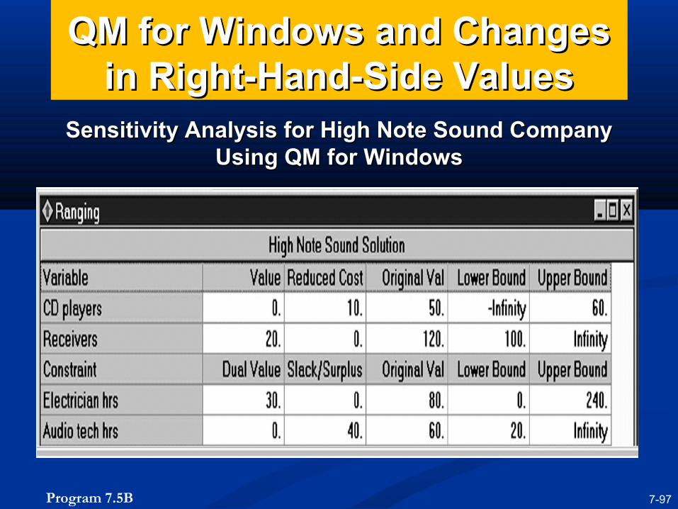
QM for Windows and Changes QM for Windows and Changes in Right-Hand-Side Valuesin Right-Hand-Side Values
Sensitivity Analysis for High Note Sound Company Sensitivity Analysis for High Note Sound Company Using QM for WindowsUsing QM for Windows
Program 7.5B
7-98
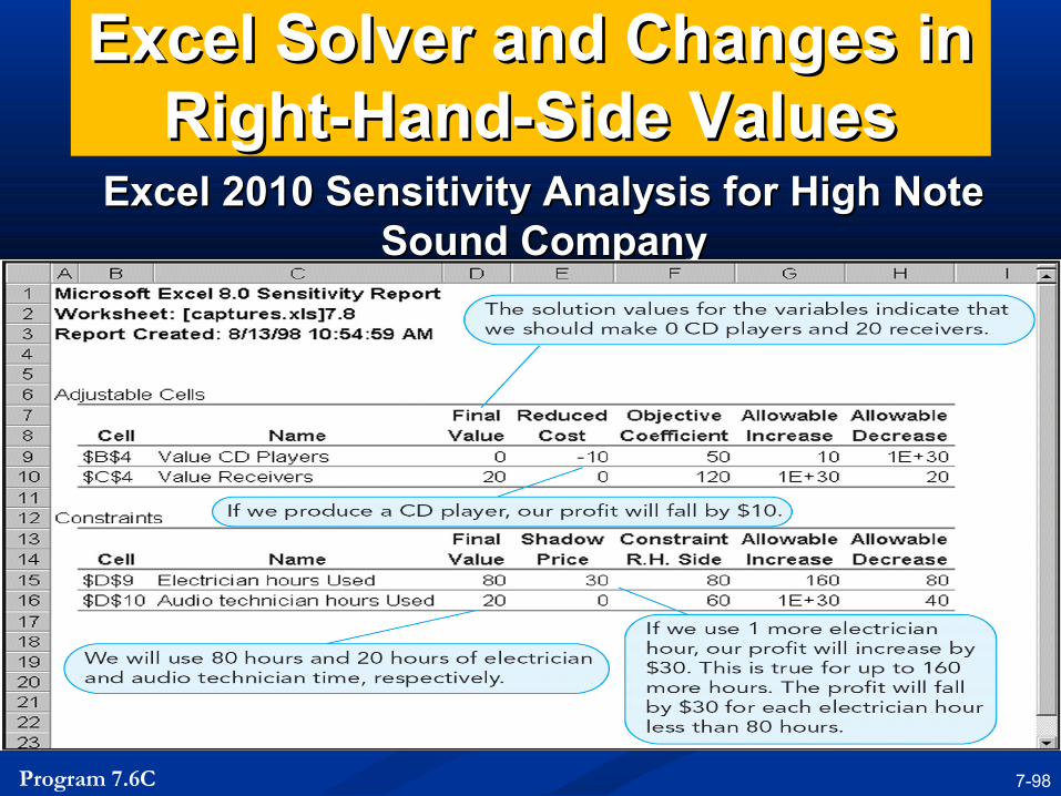
Excel Solver and Changes in Excel Solver and Changes in Right-Hand-Side ValuesRight-Hand-Side Values
Excel 2010 Sensitivity Analysis for High Note Excel 2010 Sensitivity Analysis for High Note Sound CompanySound Company
Program 7.6C
TutorialTutorial
Lab Practical : Spreadsheet Lab Practical : Spreadsheet
1 - 99
Further ReadingFurther Reading
Render, B., Stair Jr.,R.M. & Hanna, M.E. (2013) Quantitative Analysis for Management, Pearson, 11th Edition
Waters, Donald (2007) Quantitative Methods for Business, Prentice Hall, 4 th Edition.
Anderson D, Sweeney D, & Williams T. (2006) Quantitative Methods For Business Thompson Higher Education, 10th Ed.

QUESTIONS?QUESTIONS?
Recommended