A. Hoecker: Statistical Issues 1CAT Physics meeting, Feb 9, 2007
Talking Statistics Impressions from the ATLAS Statistics WS, Jan 2007
Andreas Hoecker (CERN)
CAT Physics meeting, Feb 9, 2007
A. Hoecker: Statistical Issues 2CAT Physics meeting, Feb 9, 2007
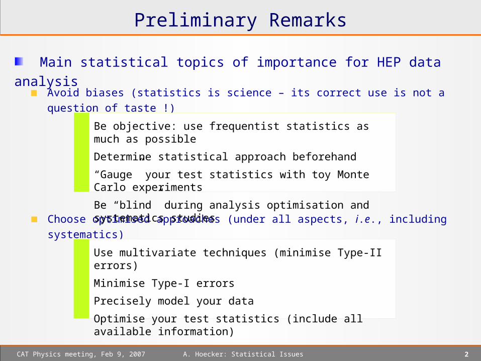
Main statistical topics of importance for HEP data analysis
Avoid biases (statistics is science – its correct use is not a question of taste !)
Choose optimised approaches (under all aspects, i.e., including systematics)
Preliminary Remarks
Be objective: use frequentist statistics as much as possible
Determine statistical approach beforehand
“Gauge” your test statistics with toy Monte Carlo experiments
Be “blind” during analysis optimisation and systematics studies
Use multivariate techniques (minimise Type-II errors)
Minimise Type-I errors
Precisely model your data
Optimise your test statistics (include all available information)

A. Hoecker: Statistical Issues 3CAT Physics meeting, Feb 9, 2007
P r e l i m i n a r i e sP r e l i m i n a r i e s
A. Hoecker: Statistical Issues 4CAT Physics meeting, Feb 9, 2007
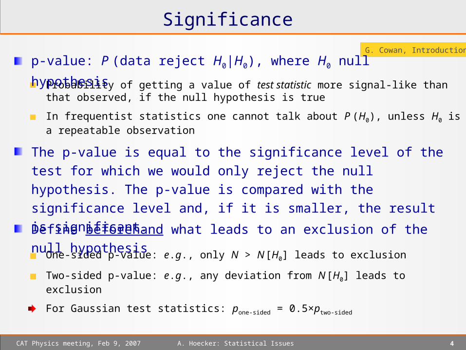
Significance
G. Cowan, Introduction
Probability of getting a value of test statistic more signal-like than that observed, if the null hypothesis is true
In frequentist statistics one cannot talk about P (H0), unless H0 is a repeatable observation
p-value: P (data reject H0|H0), where H0 null hypothesis
One-sided p-value: e.g., only N > N [H0] leads to exclusion
Two-sided p-value: e.g., any deviation from N [H0] leads to exclusion
For Gaussian test statistics: pone-sided = 0.5×ptwo-sided
The p-value is equal to the significance level of the test for which we
would only reject the null hypothesis. The p-value is compared with the
significance level and, if it is smaller, the result is significant.
Define beforehand what leads to an exclusion of the null hypothesis
A. Hoecker: Statistical Issues 5CAT Physics meeting, Feb 9, 2007
Kinds of Errors in Statistical Interpretation
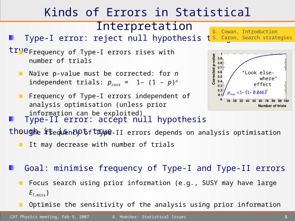
Type-I error: reject null hypothesis though it is true G. Cowan, IntroductionS. Caron, Search strategies …
Frequency of Type-I errors rises with number of trials
Naïve p-value must be corrected: for n independent trials: pcorr = 1– (1 – p)n
Frequency of Type-I errors independent of analysis optimisation (unless prior information can be exploited)
The frequency of Type-II errors depends on analysis optimisation
It may decrease with number of trials
Type-II error: accept null hypothesis though it is not true
Goal: minimise frequency of Type-I and Type-II errors
Focus search using prior information (e.g., SUSY may have large ET,miss)
Optimise the sensitivity of the analysis using prior information
corr 1 1 0.046n
p
“Look else-where effect”
A. Hoecker: Statistical Issues 6CAT Physics meeting, Feb 9, 2007
Frequentist versus Subjective (Bayesian)
G. Cowan, Introduction
The true outcome of an event is fixed but not known and cannot be known
The tools of frequentist statistics tell us what to expect, under the assumption of certain probabilities, about hypothetical repeated observations
Frequentist confidence levels (CLs) are straightforwardly obtained from toy MC samples
The nuisance parameters in these toys must be set such that the lowest CLs are obtained
Confidence levels determine exclusion probabilities. If in presence of nuisance parameters a measurement gave x ± , this does not mean that x is the most probable value !
Frequentist probability defines an event's probability as
the limit of its relative frequency in a large number of trials
Subjective Bayesian statistics gives the probability of x to take some value
It is the result of a convolution of input PDFs for all observables and nuisance parameters
The “posterior” result is subjective w.r.t. the arbitrary prior PDFs, bounds and parameterisations used
It is extremely difficult to reproduce a Bayesian result w/o having all the subjective details
A. Hoecker: Statistical Issues 7CAT Physics meeting, Feb 9, 2007
A Frequentist Analysis
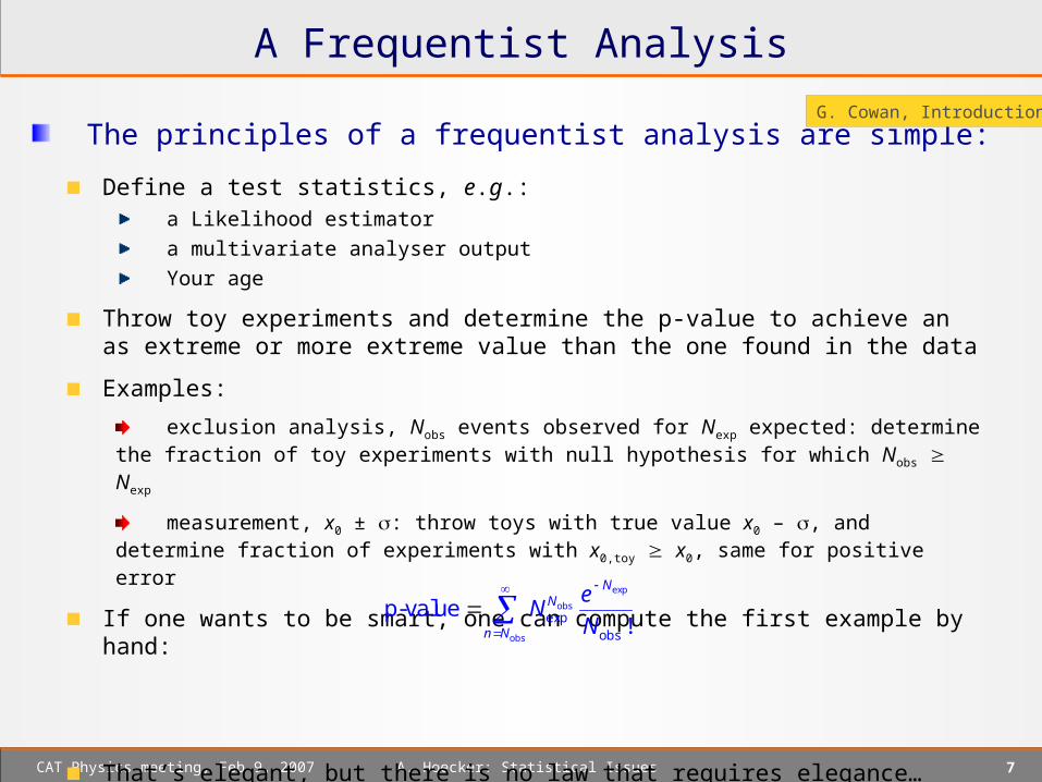
The principles of a frequentist analysis are simple:
Define a test statistics, e.g.: a Likelihood estimator
a multivariate analyser output
Your age
Throw toy experiments and determine the p-value to achieve an as extreme or more extreme value than the one found in the data
Examples:
exclusion analysis, Nobs events observed for Nexp expected: determine the fraction of toy experiments with null hypothesis for which Nobs Nexp
measurement, x0 ± : throw toys with true value x0 – , and determine fraction of experiments with x0,toy x0, same for positive error
If one wants to be smart, one can compute the first example by hand:
That’s elegant, but there is no law that requires elegance…
exp
obs
obs
expobs
p-value!
NN
n N
eN
N
G. Cowan, Introduction
A. Hoecker: Statistical Issues 8CAT Physics meeting, Feb 9, 2007
More Complicated
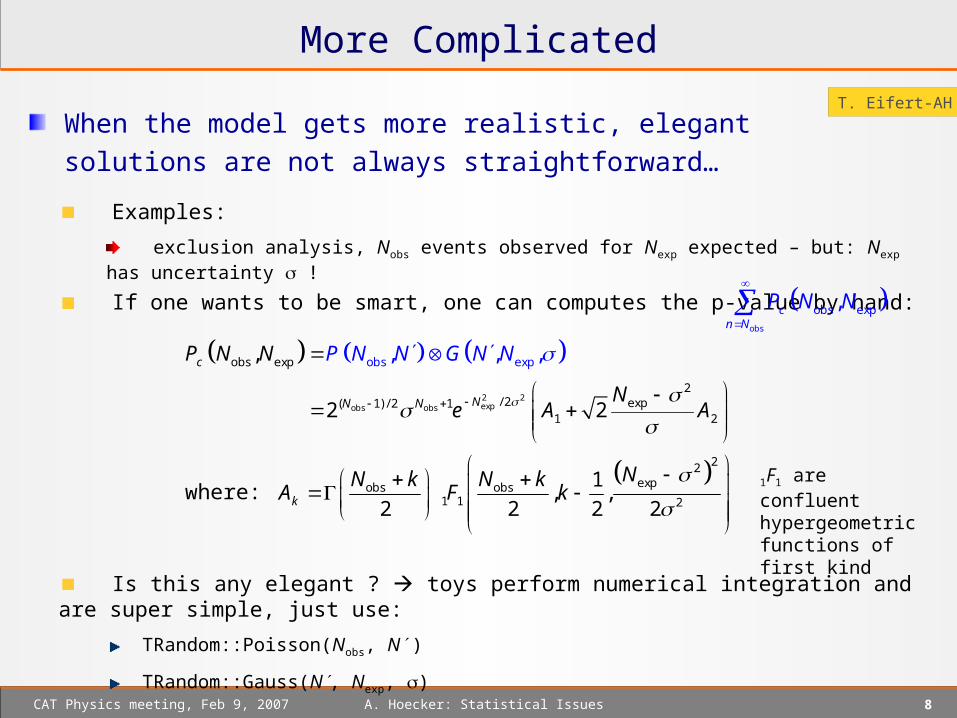
When the model gets more realistic, elegant solutions are not
always straightforward…
Examples:
exclusion analysis, Nobs events observed for Nexp expected – but: Nexp has uncertainty !
If one wants to be smart, one can computes the p-value by hand:
2 2expobs obs
obs exp
2/ 2 exp( 1) /
obs exp
2 11 2
,
2 2
, , ,c
NN N
PP N N
NA
N
A
N N G N
e
22expobs obs
1 1 2
1 , ,
2 2 2 2k
NN k N kA F k
Is this any elegant ? toys perform numerical integration and are super simple, just use:
TRandom::Poisson(Nobs, N )
TRandom::Gauss(N, Nexp, )
1F1 are confluent hypergeometric functions of first kind
where:
obs
obs exp,cn N
P N N
T. Eifert-AH
A. Hoecker: Statistical Issues 9CAT Physics meeting, Feb 9, 2007
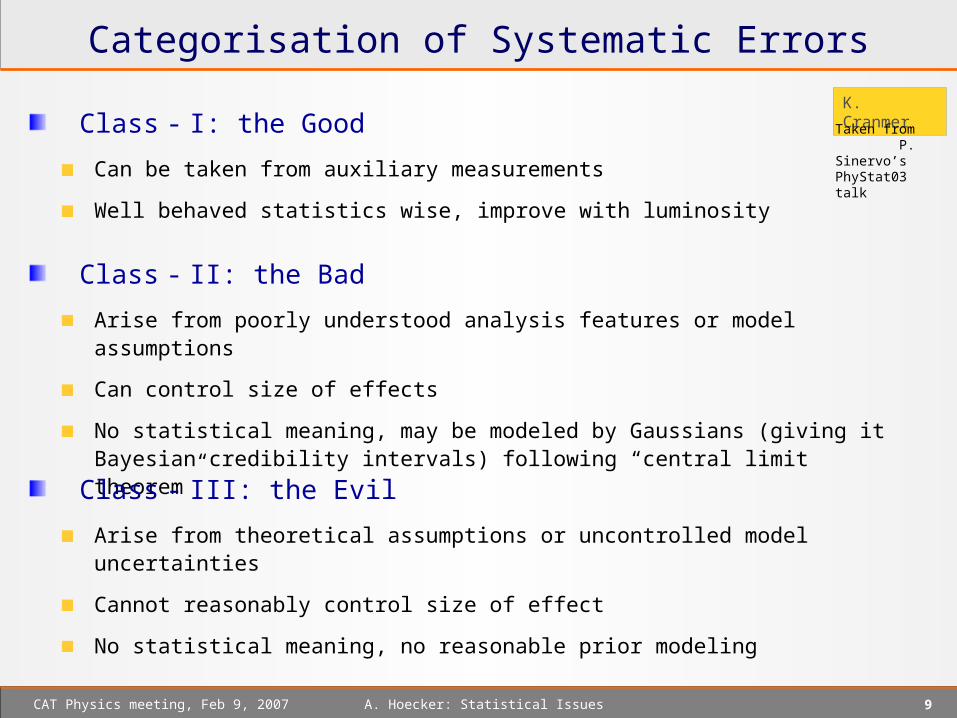
Categorisation of Systematic Errors
K. Cranmer
Class - I: the Good
Can be taken from auxiliary measurements
Well behaved statistics wise, improve with luminosity
Class - II: the Bad
Arise from poorly understood analysis features or model assumptions
Can control size of effects
No statistical meaning, may be modeled by Gaussians (giving it Bayesian credibility intervals) following “central limit theorem”
Class - III: the Evil
Arise from theoretical assumptions or uncontrolled model uncertainties
Cannot reasonably control size of effect
No statistical meaning, no reasonable prior modeling
Taken from P. Sinervo’s PhyStat03 talk
A. Hoecker: Statistical Issues 10CAT Physics meeting, Feb 9, 2007
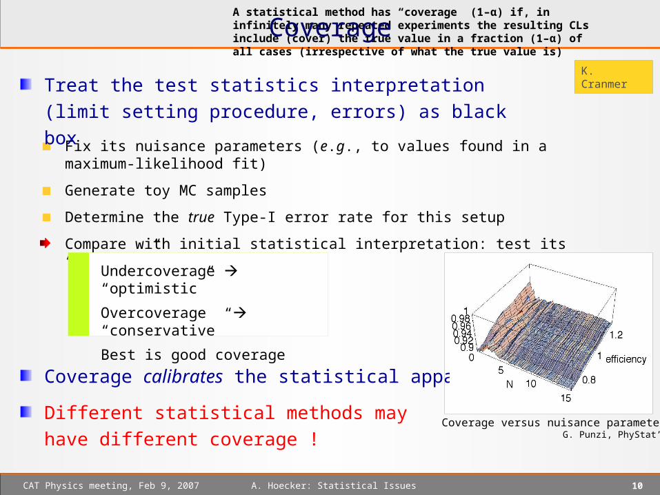
A statistical method has “coverage” (1–α) if, in infinitely many repeated experiments the resulting CLs include (cover) the true value in a fraction (1–α) of all cases (irrespective of what the true value is)Coverage
K. Cranmer
Fix its nuisance parameters (e.g., to values found in a maximum-likelihood fit)
Generate toy MC samples
Determine the true Type-I error rate for this setup
Compare with initial statistical interpretation: test its “coverage”
Treat the test statistics interpretation (limit setting procedure,
errors) as black box
Coverage calibrates the statistical apparatus
Undercoverage “optimistic”
Overcoverage “conservative”
Best is good coverage
Different statistical methods may have
different coverage !Coverage versus nuisance parameters
G. Punzi, PhyStat’05

A. Hoecker: Statistical Issues 11CAT Physics meeting, Feb 9, 2007
A p p l i c a t i o n sA p p l i c a t i o n s
A. Hoecker: Statistical Issues 12CAT Physics meeting, Feb 9, 2007
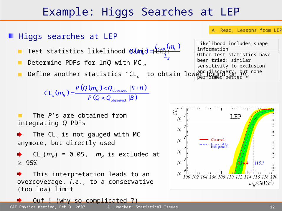
Example: Higgs Searches at LEP
A. Read, Lessons from LEP
Test statistics likelihood ratio (LR):
Determine PDFs for lnQ with MC
Define another statistics “CLs” to obtain lower bound on mH
Higgs searches at LEP
S B HH
B
L mQ m
L
Other test statistics have been tried: similar sensitivity to exclusion and discovery, but none performed better
observed
sobserved
| + CL
|H
H
P Q m Q S Bm
P Q Q B
The P’s are obtained from integrating Q PDFs
The CLs is not gauged with MC anymore, but directly used
CLs(mH) = 0.05, mH is excluded at 95%
This interpretation leads to an overcoverage, i.e., to a conservative (too low) limit
Ouf ! (why so complicated ?)
Likelihood includes shape information
A. Hoecker: Statistical Issues 13CAT Physics meeting, Feb 9, 2007
Example: Lessons from TEVATRON
Tom Junk gave an interesting talk about lessons from Tevatron. Many concrete examples of statistics use cases and pitfalls (some touched in this résumé). Too rich to summarise here. Have a look yourself !
T. Junks, Lessons from Tevatron
A. Hoecker: Statistical Issues 14CAT Physics meeting, Feb 9, 2007
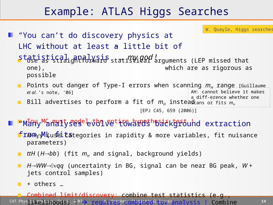
Example: ATLAS Higgs Searches
W. Quayle, Higgs searches
Use as straightforward statistical arguments (LEP missed that one), which are as rigorous as possible
Points out danger of Type-I errors when scanning mH range [Guillaume et al.’s note, ‘06]
Bill advertises to perform a fit of mH instead [EPJ C45, 659 (2006)]
Toy MC must model the entire hypothesis test !
“You can’t do discovery physics at LHC without at
least a little bit of statistical analysis” … my god !
AH: cannot believe it makes a diff-erence whether one scans or fits mH
“Many analyses evolve towards background extraction from ML fits”
H (use categories in rapidity & more variables, fit nuisance parameters)
ttH (Hbb) (fit mH and signal, background yields)
HWWqq (uncertainty in BG, signal can be near BG peak, W + jets control samples)
+ others …
Combined limit/discovery: combine test statistics (e.g., likelihoods) ? requires combined toy analysis ! Combine confidence levels ? not unambiguous ! Hot topic, I guess !
A. Hoecker: Statistical Issues 15CAT Physics meeting, Feb 9, 2007
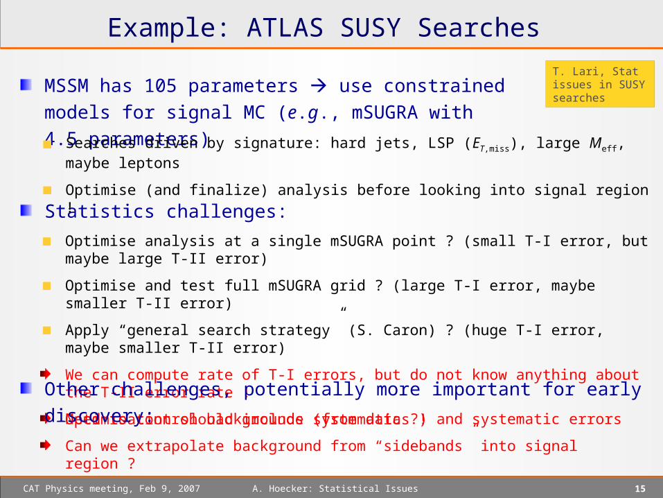
Example: ATLAS SUSY Searches
T. Lari, Stat issues in SUSY searches
Optimise analysis at a single mSUGRA point ? (small T-I error, but maybe large T-II error)
Optimise and test full mSUGRA grid ? (large T-I error, maybe smaller T-II error)
Apply “general search strategy” (S. Caron) ? (huge T-I error, maybe smaller T-II error)
We can compute rate of T-I errors, but do not know anything about the T-II error rate !
Optimisation should include systematics !
MSSM has 105 parameters use constrained models
for signal MC (e.g., mSUGRA with 4.5 parameters)
Statistics challenges:
Need to control backgrounds (from data ?) and systematic errors
Can we extrapolate background from “sidebands” into signal region ?
Other challenges, potentially more important for early discovery:
Searches driven by signature: hard jets, LSP (ET,miss), large Meff, maybe leptons
Optimise (and finalize) analysis before looking into signal region !
A. Hoecker: Statistical Issues 16CAT Physics meeting, Feb 9, 2007
A n a l y s i s O p t i m i s a t i o nA n a l y s i s O p t i m i s a t i o n
A. Hoecker: Statistical Issues 17CAT Physics meeting, Feb 9, 2007
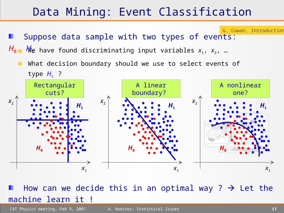
A linear boundary? A nonlinear one?
G. Cowan, Introduction
Data Mining: Event Classification
Suppose data sample with two types of events: H0, H1
We have found discriminating input variables x1, x2, …
What decision boundary should we use to select events of type H1 ?
Rectangular cuts?
H1
H0
x1
x2 H1
H0
x1
x2 H1
H0
x1
x2
How can we decide this in an optimal way ? Let the machine learn it !
A. Hoecker: Statistical Issues 18CAT Physics meeting, Feb 9, 2007
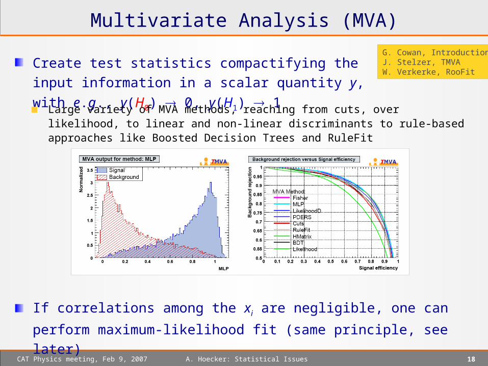
Multivariate Analysis (MVA)
G. Cowan, IntroductionJ. Stelzer, TMVAW. Verkerke, RooFit
Create test statistics compactifying the input information
in a scalar quantity y, with e.g., y(H0) 0, y(H1) 1
If correlations among the xi are negligible, one can perform maximum-
likelihood fit (same principle, see later)
Large variety of MVA methods, reaching from cuts, over likelihood, to linear and non-linear discriminants to rule-based approaches like Boosted Decision Trees and RuleFit
A. Hoecker: Statistical Issues 19CAT Physics meeting, Feb 9, 2007
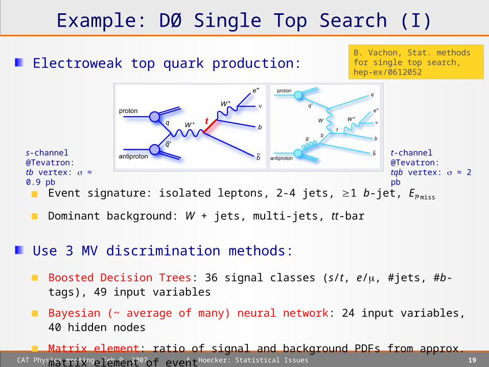
Example: DØ Single Top Search (I)
B. Vachon, Stat. methods for single top search, hep-ex/0612052
Electroweak top quark production:
t-channel @Tevatron: tqb vertex: ≈ 2 pb
s-channel @Tevatron: tb vertex: ≈ 0.9 pb
Use 3 MV discrimination methods:
Event signature: isolated leptons, 2-4 jets, 1 b-jet, ET,miss
Dominant background: W + jets, multi-jets, tt-bar
Boosted Decision Trees: 36 signal classes (s/t, e/, #jets, #b-tags), 49 input variables
Bayesian (~ average of many) neural network: 24 input variables, 40 hidden nodes
Matrix element: ratio of signal and background PDFs from approx. matrix element of event
A. Hoecker: Statistical Issues 20CAT Physics meeting, Feb 9, 2007
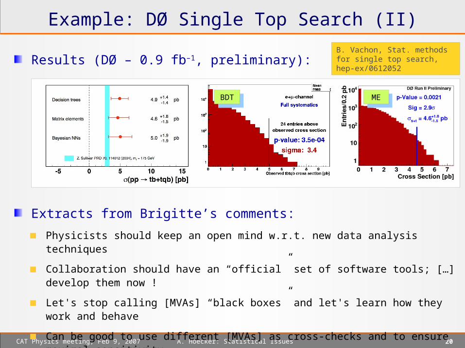
Example: DØ Single Top Search (II)
Results (DØ – 0.9 fb–1, preliminary):
Extracts from Brigitte’s comments:
Physicists should keep an open mind w.r.t. new data analysis techniques
Collaboration should have an “official” set of software tools; […] develop them now !
Let's stop calling [MVAs] “black boxes” and let's learn how they work and behave
Can be good to use different [MVAs] as cross-checks and to ensure maximal sensitivity
Most important thing is understanding of data/background modeling, not the MVA you use
B. Vachon, Stat. methods for single top search, hep-ex/0612052
BDTBDT MEME
A. Hoecker: Statistical Issues 21CAT Physics meeting, Feb 9, 2007
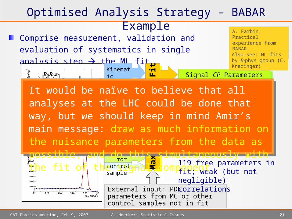
Optimised Analysis Strategy – BABAR Example
A. Farbin, Practical experience from BABAR(figure modified)
Comprise measurement, validation and evaluation of
systematics in single analysis step the ML fit
B 0h+h’- signal
candidates
Signal/Background YieldsSignal/Background Yields
Background PDF parametersBackground PDF parameters
Control sampleSignal PDF parametersSignal PDF parameters
Signal CP Parameters (blind)Signal CP Parameters (blind)Kinematic variables
PID variables
MVA
Flavour Tagging
Ma
xim
um
Lik
elih
oo
d F
it
External input: PDF parameters from MC or other control samples not in fit
Same variables for control sample 119 free parameters in fit; weak
(but not negligible) correlations
Also see: ML fits by B-phys group (E. Kneringer)
It would be naïve to believe that all analyses at the LHC could be done that way, but we should keep in mind Amir’s main message: draw as much information on the nuisance parameters from the data as possible, and do this simultaneously with the fit of the signal component
A. Hoecker: Statistical Issues 22CAT Physics meeting, Feb 9, 2007
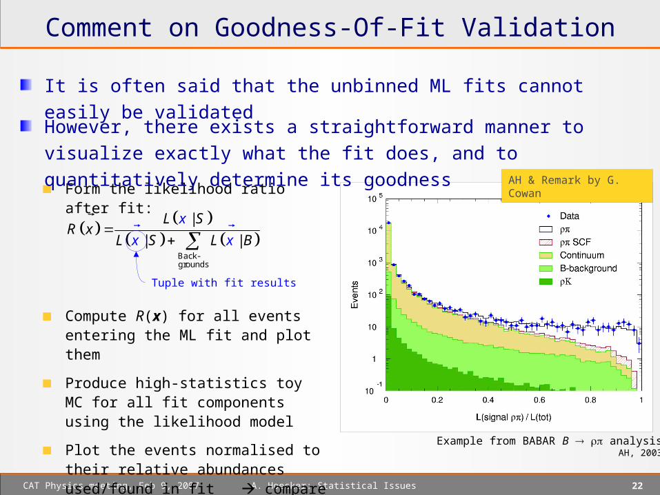
Comment on Goodness-Of-Fit Validation
It is often said that the unbinned ML fits cannot easily be validated
Form the likelihood ratio after fit:
Compute R(x) for all events entering the ML fit and plot them
Produce high-statistics toy MC for all fit components using the likelihood model
Plot the events normalised to their relative abundances used/found in fit compare !
Back-grounds
|
| |
L SR x
L S L B
x
x x
Tuple with fit results
Example from BABAR B analysisAH, 2003
However, there exists a straightforward manner to visualize exactly what
the fit does, and to quantitatively determine its goodnessAH & Remark by G. Cowan

A. Hoecker: Statistical Issues 23CAT Physics meeting, Feb 9, 2007
S t a t i s t i c s T o o l k i t sS t a t i s t i c s T o o l k i t s
A. Hoecker: Statistical Issues 24CAT Physics meeting, Feb 9, 2007
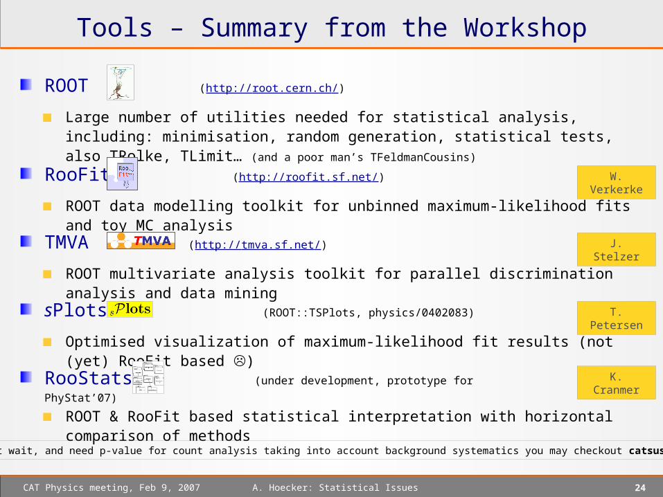
Tools – Summary from the Workshop
ROOT (http://root.cern.ch/)
Large number of utilities needed for statistical analysis, including: minimisation, random generation, statistical tests, also TRolke, TLimit… (and a poor man’s TFeldmanCousins)
RooFit (http://roofit.sf.net/)
ROOT data modelling toolkit for unbinned maximum-likelihood fits and toy MC analysis
W. Verkerke
TMVA (http://tmva.sf.net/)
ROOT multivariate analysis toolkit for parallel discrimination analysis and data mining
J. Stelzer
sPlots (ROOT::TSPlots, physics/0402083)
Optimised visualization of maximum-likelihood fit results (not (yet) RooFit based )
T. Petersen
RooStats (under development, prototype for PhyStat’07)
ROOT & RooFit based statistical interpretation with horizontal comparison of methods
K. Cranmer
If you can’t wait, and need p-value for count analysis taking into account background systematics you may checkout catsusy/StatTools

A. Hoecker: Statistical Issues 25CAT Physics meeting, Feb 9, 2007
B l i n d A n a l y s i sB l i n d A n a l y s i s
A. Hoecker: Statistical Issues 26CAT Physics meeting, Feb 9, 2007
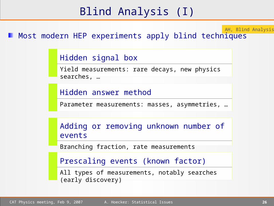
Hidden signal box
Yield measurements: rare decays, new physics searches, …
Adding or removing unknown number of events
Branching fraction, rate measurements
Prescaling events (known factor)
All types of measurements, notably searches (early discovery)
Hidden answer method
Parameter measurements: masses, asymmetries, …
Blind Analysis (I)
AH, Blind Analysis
Most modern HEP experiments apply blind techniques
A. Hoecker: Statistical Issues 27CAT Physics meeting, Feb 9, 2007
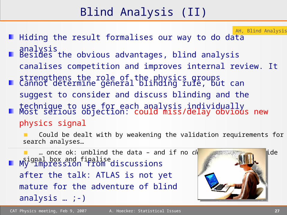
Blind Analysis (II)
AH, Blind Analysis
Cannot determine general blinding rule, but can suggest to consider and
discuss blinding and the technique to use for each analysis individually
Hiding the result formalises our way to do data analysis
Most serious objection: could miss/delay obvious new physics signal Could be dealt with by weakening the validation requirements for search analyses…
… once ok: unblind the data – and if no clear-cut signal, re-hide signal box and finalise
Besides the obvious advantages, blind analysis canalises competition and
improves internal review. It strengthens the role of the physics groups
My impression from discussions after the talk:
ATLAS is not yet mature for the adventure of
blind analysis … ;-)
A. Hoecker: Statistical Issues 28CAT Physics meeting, Feb 9, 2007
C o n c l u s i o n sC o n c l u s i o n s
Need to detain our statistics enthusiasm and first understand: …the detector response
…the basic QCD processes and other backgrounds
…and validate the MC simulation
Fortunately: optimised analysis also helps to reduce background systematics !
Daniel doesn’t adhere to frequentist vs. Bayesian discussions, and he
doesn’t seem to like nuisance parameters either ;-)
“Today we have acquired far more sophisticated tools than twenty years
ago, but we do not write them always ourselves, which often entails the
risk that we do not test them adequately” MC generators, analysis
tools !
D. Froidevaux’s “Motherhood statements”
(AH)
Statistics working group contacts with CMS being prepared (by whom?)
Inter-experiment combination should not wait years to be started A. Read
Recommended