SWAT Modeling of the Arroyo Colorado Watershed
Narayanan Kannan, Ph.D.
Texas Water Resources InstituteTR-426
June 2012

SWAT MODELING OF
THE ARROYO COLORADO WATERSHED
Narayanan Kannan, Ph.D. Assistant Research Scientist-Texas AgriLife Research
Blackland Research and Extension Center
Temple, TX, 76502
Texas Water Resources Institute
Technical Report No. 426
June 2012
Arroyo Colorado Agricultural Nonpoint Source Assessment
The report highlights the accomplishment of Task 8 of TSSWCB Project number 06-10
This report was created through the Arroyo Colorado Agricultural Nonpoint Source Assessment
project funded by the United States Environmental Protection Agency through a Clean Water
Act §319(h) grant administered by the Texas State Soil and Water Conservation Board
(TSSWCB).

SWAT MODELING OF THE ARROYO COLORADO WATERSHED Page 2
TABLE OF CONTENTS
Summary 3
Purpose and scope 4
Introduction 4
Study area 6
Observations used 8
Description of simulation model 10
SWAT model setup of Arroyo Colorado watershed 14
Input data used 14
Modeling irrigation of crops 15
Representing Best Management Practices (BMPs) in the model 16
Calibration and validation of model 23
Watershed scenarios for 2015 and 2025 24
Estimation of land cover maps for 2015 and 2025 24
Development of model input files for future scenarios 26
Analysis of present and future dissolved oxygen trends 27
Discussion of mitigation of dissolved oxygen problems 30
Acknowledgements 32
References 33
Appendix 36

SWAT MODELING OF THE ARROYO COLORADO WATERSHED Page 3
Summary
A model setup of the Soil and Water Assessment Tool (SWAT) watershed model was developed to
simulate flow and selected water quality parameters for the Arroyo Colorado watershed in South Texas.
The model simulates flow, transport of sediment and nutrients, water temperature, dissolved oxygen, and
biochemical oxygen demand. The model can also be used to estimate a total maximum daily load for the
selected water quality parameters in the Arroyo Colorado. The model was calibrated and tested for flow
with data measured during 2000–2009 at two streamflow-gaging stations. The flow was calibrated
satisfactorily at monthly and daily intervals. In addition, the model was calibrated and tested sequentially
for suspended sediment, orthophosphate, total phosphorus, nitrate nitrogen, ammonia nitrogen, total
nitrogen, and dissolved oxygen, using data from 2000–2009. The simulated loads or concentrations of the
selected water quality constituents generally matched the measured counterparts available for the
calibration and validation periods. Two watershed scenarios were simulated for the years 2015 and 2025
after estimation of land cover maps for those years. The scenarios were intended to identify a suite of best
management practices (BMPs) to address the depressed dissolved oxygen problem in the watershed.

SWAT MODELING OF THE ARROYO COLORADO WATERSHED Page 4
Purpose and Scope
This report describes the setup, calibration, validation, and scenario analysis using the SWAT model to
simulate the flow and water quality of the Arroyo Colorado watershed. The basin was subdivided into 17
subbasins—six in Segment 2201 and eleven in Segment 2202. The basin was characterized by a set of
475 hydrologic response units (HRUs) that are unique combinations of land cover, soil, and slope. For
flow, 8 hydrologic process-related parameters were calibrated. A total of 26 process-related parameters
were calibrated for water quality. Eleven years (1999–2009) of precipitation, air temperature, streamflow,
and water-quality data were used for model calibration and validation. We used precipitation data from
three stations; air temperature data from two stations; and streamflow data from two stations. Most of the
water quality data used for model calibration and testing came from the station near Harlingen, Texas.
Some water quality data available near Mercedes, Texas were also used in the study. Status of water
quality in the river at present and for years 2015 and 2025 were projected using estimated land cover
maps. Suggested solutions to bring dissolved oxygen in compliance for the stream were also discussed.
Introduction
The Arroyo Colorado watershed, a subwatershed of the Nueces-Rio Grande Coastal Basin, is located in
the Lower Rio Grande Valley of South Texas and extends from near Mission, Texas, eastward to the
Laguna Madre (fig. 1). Streamflow in the Arroyo Colorado primarily is sustained by municipal and
industrial effluents. Additional streamflow results from irrigation return flow, rainfall runoff, and other
point-source discharges. The Arroyo Colorado is used as a floodway, an inland waterway, and a
recreational area for swimming, boating, and fishing, and is an important nursery and foraging area for
shrimp, crab, and several types of marine fish.
The Texas Commission on Environmental Quality (TCEQ) has classified two reaches of the Arroyo
Colorado based on the physical characteristics of the stream. Segment 2201, from the Port of Harlingen to
the confluence with the Laguna Madre, is tidally influenced and has designated uses of contact recreation
and high aquatic life. The nontidal segment of the Arroyo Colorado, Segment

SWAT MODELING OF THE ARROYO COLORADO WATERSHED Page 5
Figure 1. Location of Arroyo Colorado watershed
SWAT MODELING OF THE ARROYO COLORADO WATERSHED Page 6
2202, has designated uses of contact recreation and intermediate aquatic life. The tidal segment of the
Arroyo Colorado, Segment 2201, has failed to meet the water quality criteria required for its designated
uses and is included on the State 303(d) list of impaired water bodies for dissolved oxygen (DO) levels
below the criteria specified in the Texas Surface Water Quality Standards (Texas Natural Resource
Conservation Commission, 1997).
Simulation models typically are used to estimate load reductions because the models are developed to
represent the cause-and-effect relations between natural inputs to an aquatic ecosystem and the resulting
water quality. Several BMP alternatives can be evaluated objectively using simulation models to
determine what changes will be needed to meet the water quality standards.
Texas AgriLife Research, in cooperation with Texas State Soil and Water Conservation Board
(TSSWCB) and TCEQ, began a study in 2008 to simulate the flow and the water quality of selected
constituents in the Arroyo Colorado. The specific objectives of the study were to (1) develop a computer-
based watershed model setup of the Arroyo Colorado that would allow representation of different BMPs
adopted by growers in the watershed; (2) calibrate and validate a set of process-related model parameters
with available streamflow and water quality data for the watershed; and (3) develop a suite of BMPs for
changing land cover conditions predicted for 2015 and 2025, which, when progressively implemented in
the watershed, would bring the water quality to compliance with current standards.
Study Area
The study area, the Arroyo Colorado watershed, is located in the Lower Rio Grande Valley of South
Texas in parts of Hidalgo, Cameron, and Willacy counties (Fig. 1). It is a subwatershed of the Nueces-Rio
Grande Coastal Basin, also known as the South (Lower) Laguna Madre Watershed (Hydrologic Unit
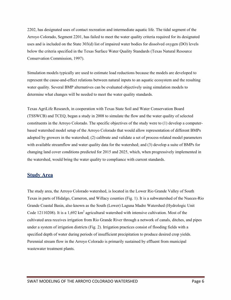
Code 12110208). It is a 1,692 km2 agricultural watershed with intensive cultivation. Most of the
cultivated area receives irrigation from Rio Grande River through a network of canals, ditches, and pipes
under a system of irrigation districts (Fig. 2). Irrigation practices consist of flooding fields with a
specified depth of water during periods of insufficient precipitation to produce desired crop yields.
Perennial stream flow in the Arroyo Colorado is primarily sustained by effluent from municipal
wastewater treatment plants.
SWAT MODELING OF THE ARROYO COLORADO WATERSHED Page 7
Figure 2. Irrigation districts in the watershed
108.18 km (64.5 miles)

SWAT MODELING OF THE ARROYO COLORADO WATERSHED Page 8
Irrigation return flow and point source discharges supplement the flow on a seasonal basis. The Arroyo
Colorado is used as a floodway, an inland waterway, and a recreational area for swimming, boating, and
fishing, and is an important nursery and foraging area for numerous marine species. Urbanization is
extensive in the areas directly adjacent to the main stem of the Arroyo Colorado, particularly in the
western and central parts of the basin. Principal urban areas include the cities of Mission, McAllen, Pharr,
Donna, Weslaco, Mercedes, Harlingen, and San Benito (Rains and Miranda, 2002; Rosenthal and Garza,
2007).
The most dominant land cover category in the watershed is agriculture (54 %) and the main crops
cultivated are grain sorghum, cotton, sugar cane, and citrus, although some vegetable and fruit crops are
also raised. Most of the cultivated area (including citrus and sugarcane) is irrigated. The watershed soils
are clays, clay loams, and sandy loams. The major soil series comprise the Harlingen, Hidalgo, Mercedes,
Raymondville, Rio Grande, and Willacy (U.S. Department of Agriculture, Soil Conservation Service,
1977, 1981–82). Most soil depths range from about 1,600 to 2,000 mm.
The mean annual temperature of the watershed is 22.7 degrees Celcius ( C) with mean monthly
temperatures ranging from 14.5 C in January to 28.9 C in July. Mean annual precipitation ranges from
about 530 to 680 mm, generally from west to east, in the basin (National Oceanic and Atmospheric
Administration, 1996). Most of the annual precipitation results from frontal storms and tropical storms.
Observations used
Twelve years of weather data and flow, beginning in 1999 to 2010, were used for modeling. We used
precipitation data from three and temperature data from two stations (Fig. 1). The weather data was
obtained from Texas State Climatologist Office located at Texas A&M University in College Station.
Stream flow data for two stations were obtained from International Boundary and Water Commission;
one near Llano Grande at FM 1015 south of Weslaco (G1) and the other near US 77 in South West
Harlingen (G2) (Table 1). There are 21 permitted dischargers in the Arroyo Colorado Basin, 16 are
municipal, three are industrial, and two are shrimp farms. The discharge permit limits of the municipal
plants range from 0.4 to 10 million gallons per day. The shrimp farms discharge infrequently (Rains and
Miranda, 2002).
SWAT MODELING OF THE ARROYO COLORADO WATERSHED Page 9
Water quality data from limited grab samples were obtained for suspended sediment (SS), nitrogen
(ammonia nitrogen (amm N), nitrate-nitrogen (NO3-N), and total nitrogen (TN)), phosphorus
(orthophosphate (OP) and total phosphorus (TP)), water temperature (WT), and dissolved oxygen (DO).
Data were available from three stations: the first near Weslaco, the second near Harlingen and the third
near Port of Harlingen (Table 1). Out of the three stations, only the station near Harlingen had data for all
the water quality variables. The gauge near Weslaco had flow, SS and, amm N only. However, the gauge
near Port of Harlingen had very limited data (<10--20 observations) for SS, amm N, and WT, and
therefore was not used for the analysis (Table 1).
The observations were available in the form of concentrations (except water temperature). The monitored
observations (concentrations) were converted to time series of loads using a continuous time series of
flow (typically daily stream flow). There are computer programs to accomplish this that convert flow and
concentrations using regression and statistical techniques. They also estimate uncertainties of estimates.
One such program is LOAD ESTimator (LOADEST) developed by United States Geological Survey
(USGS) (Runkel et al. 2004). In LOADEST, data variables such as various functions of flow, time, and
some other user-specified variables can be included. The program develops a regression model for
estimation of load after calibration. Once formulated, the regression model is then used to estimate loads
for a user-specified time frame. The LOADEST program estimates mean loads, standard errors, and 95 %
confidence intervals developed on a monthly or seasonal basis. LOADEST output includes diagnostic
tests and warnings to the user in determining correct estimation procedure and ways to interpret the
information obtained. The time series of pollutants estimated this way using LOADEST based on grab
sample pollutant concentrations and flow is referred to as “observations” throughout this report.

SWAT MODELING OF THE ARROYO COLORADO WATERSHED Page 10
Description of simulation model
The Soil and Water Assessment Tool (SWAT) (Arnold et al. 1993) is a conceptual continuous simulation
model developed to quantify the impact of land management practices on surface water quality in large
watersheds (Gassman et al. 2007; Neitsch et al. 2004; http://www.brc.tamus.edu/swat).
Table 1. Selected physical and hydrological characteristics of Arroyo Colorado subbasins
SubBasin Reach
length
(km)
Drainage
area
(Km2)
Name of
precipitation
station
Streamflow
gauging station
number
Water quality
sampling site
number
(Segment 2202 non-tidal)
2 11.5 50.3
3 11.5 73.8 Mc Allen
4 16.7 157.4
5 9.0 57.7
6 10.0 82.6 Mercedes 08-4703.00 13081
7 10.8 100.3
8 19.6 143.3
9 10.1 47.5 Harlingen
10 12.7 104.9 08-4704.00 13074
11 20.3 96.9
12 10.6 155.8
(Segment 2201 tidal)
13 10.0 59.4
14 8.8 59.2
15 53.4 249.0
16 7.4 54.3
17 25.6 110.2
1 8.5 89.8

SWAT MODELING OF THE ARROYO COLORADO WATERSHED Page 11
Figure 3. Land cover map of Arroyo Colorado
108.18 km (64.5 miles)

SWAT MODELING OF THE ARROYO COLORADO WATERSHED Page 12
Figure 4. Soil map of the watershed
108.18 km (64.5 miles)

SWAT MODELING OF THE ARROYO COLORADO WATERSHED Page 13
Table 2. Land cover map legend descriptions
Land Cover Code Description
AGRL
AGRR
FRST
ORCD
PAST
RNGB
RNGE
SUGC
UCOM
UIDU
UINS
URHD
URLD
URML
UTRN
WATR
WETF
WETN
Generic Agricultural Land
Agricultural Land-Row Crops
Mixed Forest
Orchard (Citrus for Arroyo Colorado watershed)
Pasture
Range-Brush
Range-Grasses
Sugarcane
Urban-Commercial facility
Urban-Industry
Urban-Institution
Urban-High Density Residential
Urban-Low Density Residential
Urban-Residential Medium/Low density
Urban-Transportation
Water
Wetland-Forested
Wetland-Non-forested
SWAT also provides a continuous simulation of processes such as evapotranspiration, surface runoff,
percolation, return transport flow, groundwater flow, channel transmission losses, pond and reservoir
storage, channel routing, field drainage, crop growth, and material transfers (soil erosion, nutrient and
organic chemical and fate). The model can be run with a daily time step, although subdaily model run is
possible with Green and Ampt infiltration method. It incorporates the combined and interacting effects of
weather and land management (e.g. irrigation, planting and harvesting operations, and the application of
fertilizers, pesticides or other inputs). SWAT divides the watershed into subwatersheds using topography.
Each subwatershed is divided into HRUs, which are unique combinations of soil, land cover and slope.
Although individual HRU’s are simulated independently from one another, predicted water and material
flows are routed within the channel network, which allows for large watersheds with hundreds or even
thousands of HRUs to be simulated.

SWAT MODELING OF THE ARROYO COLORADO WATERSHED Page 14
SWAT model setup of Arroyo Colorado watershed
Input data used
We used ArcSWAT interface to prepare the SWAT model setup of Arroyo Colorado. For delineation of
watershed boundary, we used 30-m USGS Digital Elevation Model (DEM). A digitized stream network
and a watershed boundary from the previous HSPF modeling study (Rains and Miranda, 2002) were used
as supporting information for the delineation of watershed and stream network for the present study. The
watershed was eventually discretized into 17 subwatersheds.
Spatial Sciences Lab of Texas A&M University at College Station prepared the land cover map based on
satellite data and a field survey. The map incorporates the present land cover conditions (2004–2007) in
the watershed. Crop rotation, irrigation, and dates of planting are also available with the land use map on
a farm/field basis. The dominant land cover categories in the watershed are agriculture (54 %), range
(18.5 %), urban (12.5 %), water bodies (6 %) and sugarcane (4 %) although some vegetable and fruit
crops are also raised (Fig. 3, Table 2). The soil survey geographic database (SSURGO) soil map was
downloaded from USDA-NRCS for Cameron, Willacy and Hidalgo counties (Fig. 4). The soil properties
associated with a particular soil type are derived using the SSURGO soil database tool. 475 HRUs were
delineated based on a combination of land cover and soil. In the present delineation, areas as small as 9.1
ha (22.5 acres) are represented as HRUs.
Dates of planting were obtained from the land cover map. The durations of crops were obtained from crop
fact sheets from Texas AgriLife Extension Service publications based on the tentative harvest dates as
identified for each crop (Stichler and McFarland, 2001; Trostle and Porter, 2001; Stichler et al. 2008;
Vegetable Team Production, 2008; Wiedenfeld and Enciso, 2008; Wiedenfeld and Sauls, 2008). Dates of
harvest collected during our visits to the watershed were used along with the above information.
Typically, there are two tillage operations (in conventional tillage) for each crop, one soon after the
harvest of the previous crop and the other midway between the harvest of the previous crop and the
planting of the present crop. In conservation tillage, one tillage operation (mostly soon after harvest of the
previous crop) or no tillage operation is performed (Andy Garza, Texas State Soil and Water
Conservation Board, Harlingen, personal communication).

SWAT MODELING OF THE ARROYO COLORADO WATERSHED Page 15
Modeling Irrigation of crops
Tentative quantity, timing, and frequency of irrigation required for major crops (such as sorghum, cotton
and sugar cane) were obtained from NRCS and TSSWCB staff in the watershed. Crop fact sheets
published by Texas AgriLife Extension Service were also collected to estimate the irrigation information
for the crops (Table 3; Stichler and McFarland, 2001; Trostle and Porter, 2001; Cruces, 2003; Fipps,
2005; Stichler et al. 2008; Vegetable Team Production, 2008; Wiedenfeld and Enciso, 2008; Wiedenfeld
and Sauls, 2008). To model canal irrigation, the following procedure is used. We prepared a
comprehensive map using the HRU information from the overlaid land cover map, soil map and subbasin
map using GIS. An HRU under agriculture land cover can be either irrigated or not irrigated. If irrigated,
the model will follow the canal irrigation procedure. Information on irrigation districts for the study area
is available in the form of a map from the Irrigation Technology Center, Texas A&M University. In
addition, the average water conveyance efficiency for each irrigation district is available separately. This
information was combined and merged with the HRU map to identify the irrigation district that comes
under each HRU. This has conveyance efficiency information for each HRU. For this study, conveyance
efficiency includes all loses in the irrigation distribution system from water diversion river to field.
Conveyance efficiency combined with depth of water application for each irrigation event for each crop
allowed us to estimate the tentative quantity of water that could have been diverted from the source for
irrigating the crop (Fig. A1). We consulted several publications/reports estimating depth, duration, and
frequency of irrigation, and estimated the critical crop growth stages at which irrigation is essential. We
also estimated the timings based on the probable days of irrigation (identified by looking at the daily
water stress values reported by the model for the simulation that involves no irrigation event for any crop
in any HRU) to schedule irrigation in the model set up, and the critical crop growth stages requiring
irrigation were used as reported in the literature/field data.

SWAT MODELING OF THE ARROYO COLORADO WATERSHED Page 16
Representing Best Management Practices (BMPs) in the model
Irrigation land leveling (NRCS practice code 464)
Irrigation land leveling represents the reshaping of the irrigated land to a planned grade to permit uniform
and efficient application of water. It is typically used in mildly sloping land. Primarily it is carried out by
agricultural producers who follow surface methods to irrigate their fields. Land leveling is generally
designed within slope limits of water irrigation methods used, provide removal of excess surface water
and control erosion caused by rainfall. This BMP is modeled in SWAT by reducing the HRU slope (by 8–
12.5 % depending on the initial value) and slope length (one tenth of the default value) parameter. In
reality, a leveled field infiltrates more water, reduces surface runoff, and therefore decreases soil erosion.
When adjusted (reduced), slope and slope length parameters of the watershed model setup will bring
similar effects in the predicted model results.
Irrigation Water Conveyance, Pipeline (NRCS practice code 430)
Irrigation water conveyance in pipeline form is installation of underground thermoplastic pipeline (and
appurtenances) as a part of an irrigation system to replace canal lining. The decision to line a canal or
replace the canal using a pipeline is often made based on how much water is conveyed in the canal. In
practice, small district irrigation canals or lateral canals with capacity less than 100 cubic feet per second
will be replaced with pipeline. This BMP reduces water conveyance losses and prevents soil erosion or
loss of water quality. Some of the design and planning considerations include working pressure, friction
losses, flow velocities, and flow capacity. On average, this BMP can save water up to 11 % (Texas Water
Development Board, report 362). In a hydrologic modeling study involving a relatively large watershed, it
is not possible to practically consider all the pipe network, irrigation appurtenances, and the associated
pressure, friction losses, flow velocity, capacity etc. Therefore, irrigation water conveyance in pipeline
form is modeled by increasing the conveyance efficiency of an HRU. In other words, the amount of water
diverted to the field from the source is decreased.
Irrigation System-Surface Surge Valves
This BMP is often implemented to replace an on-farm ditch with a gated pipeline to distribute water to
furrow irrigated fields. A surge irrigation system applies water intermittently to furrows to create a series
of on-off periods of either constant or variable time intervals. The system includes butterfly valves or
similar equipment that will provide equivalent alternating flows with adjustable time periods. Surge flow
reduces runoff by increasing uniformity of infiltration and by reducing the duration of flow as the water
reaches the end of the field. It also increases the amount of water delivered to each row and reduces deep

SWAT MODELING OF THE ARROYO COLORADO WATERSHED Page 17
percolation of irrigation water near the head of the field. The amount of water saved by switching to surge
flow is estimated to be between 10 and 40 % (Texas Water Development Board, report 362) and is
dependent upon soil type and timing of operations. Physical representation and modeling the operation of
butterfly values for each field in a large watershed system was tedious. Also, methods do not exist to
model them from a hydrologic perspective. Therefore, irrigation system-surface surge valves is simulated
by increasing the conveyance efficiency while calculating the water diverted for irrigation.
Irrigation Water Management (NRCS practice code 449)
Under this BMP, the landowner will manage the volume, frequency, and application rate of irrigation in a
planned, efficient manner as determined from the crop’s water requirements complying with federal,
state, and local laws and regulations. This BMP is modeled by varying several parameters. The volume of
water required for irrigation is adjusted based on the seasonal total rainfall received (total rainfall from
planting to harvest date).. If there is considerable rainfall around a scheduled irrigation period, that
particular irrigation is skipped. This reduces the frequency of irrigation. Based on the quantity of rainfall
and timing, the rate of water application is also adjusted, although this is less frequent.

SWAT MODELING OF THE ARROYO COLORADO WATERSHED Page 18
Table 3. Frequency, timing and amount of irrigation for different crops in the watershed
Table 4. Water Diverted for Irrigation with and without BMPs
Subbasin Year Crop Water diverted
without BMPs mm (in.)
Water diverted
with BMPs mm (in.)
3
3
8
8
8
2002
2004
2000
2001
2002
Sugarcane
Sugarcane
Cotton
Corn
Cotton
1,524 (60)
1,052 (41)
677 (27)
677 (27)
677 (27)
1,160 (46)
801 (32)
552 (22)
552 (22)
552 (22)
Crop
Total water
requirement,
mm (inches)
Number of
irrigations
Critical crop growth stages needing irrigation
Irrigation requirement (Days
after planting)
Sorghum
Cotton
Sugarcane
Corn
Citrus
Sunflower
Onion
458 (18)
508 (20)
1270 (50)
508 (20)
1143 (45)
304 (12)
635 (25)
3
3
7
3
6
2
5
One week before booting, two weeks past flowering
Stand establishment, prebloom, shortly after boll set
Establishment, grand growth, ripening
Tasseling, silking, kernel fill
Pre-bloom, flower bud induction, fruit set, cell expansion, ripening
20 days before flowering, 20 days after flowering
stand establishment, bulb initiation, maturity
30, 60, 84
25, 56, 94
75, 105, 145, 190, 235, 275, 305
48, 70, 95
65, 100, 135, 195, 250, 320
45, 85
15, 60 (if dry), 90, 115, 135

SWAT MODELING OF THE ARROYO COLORADO WATERSHED Page 19
Conservation Crop Rotation (NRCS practice code 328)
This BMP implies growing high-residue-producing crops that produce a minimum of 2800 kg/ha/year
(2500 lbs/ac/year) of residue for a minimum of 1 year within a given two year period. Corn and grain
sorghum are examples for high-residue-producing crops. Sorghum is the dominant crop in cultivated
areas of the watershed. Corn is also cultivated in some areas. The crop rotation in the watershed has
sorghum, or corn as per the above-mentioned conditions prescribed for conservation crop rotation.
Therefore, no changes were made in the watershed model set up to represent this BMP.
Nutrient Management (NRCS practice code 590)
Nutrient management means managing fertilizer quantity, placement, and timing based on realistic yield
goals and moisture prospects. Under this BMP, fertilizer should be applied in split applications
throughout the year (early March, late May, late August, and mid October) prior to irrigation or
forecasted rain to maximize the use of the fertilizer and minimize the leaching potential. Nitrogen
applications will not exceed 112 kg/ha (100 lb/ac) of total nitrogen per application. Specific nutrient
recommendations will be given by NRCS when a soil analysis report is provided. A soil analysis is taken
a minimum of once every third year by the land owner/renter beginning with the year that the plan or
contract is signed. Nutrient management is mimicked in the model as given below.
The fertilizer applications for cultivated fields were already modeled in terms of two or three split
applications. For the HRUs that come under this BMP, the split applications were strictly followed
according to the guidelines suggested in the BMP practice code. In addition, the initial amount of N and
P present in the soil were deducted from the recommended regular fertilizer application rates for different
crops (to mimic soil-survey based N and P recommendations). Realistic initial N and P rates were
obtained by using the final amount of N and P remaining in the soil (as reported by the model) after
several years of model runs. With respect to recommended regular rates of N and P, under this
management scenario, less proportion of P than N is applied .. This is because phosphorus is less likely
to leach from the soil and more available. A comparison of N and P rates for different crops with and
without nutrient management is given in Table 5.

SWAT MODELING OF THE ARROYO COLORADO WATERSHED Page 20
Table 5. Fertilizer rates for different crops under nutrient management and non-nutrient management
Crop
Nitrogen (kg/ha) Phosphorus (kg/ha)
Regular Nutrient
management
Regular Nutrient
management
Sorghum
Cotton
Sugarcane
160
150
224
152
125
216
69
68
0
55
34
0
Residue Management (NRCS practice code 329b)
Residue management-mulch-till is managing the amount, orientation, and distribution of crop and other
plant residue on the soil surface year-round while growing crops. The entire field surface is tilled prior to
the planting operation. Sometimes the residue is partially incorporated using chisels, sweeps, field
cultivators, or similar implements. This BMP is practiced as part of a conservation management strategy
to achieve some/all of the following: reduce sheet and rill erosion, reduce wind erosion, maintain or
improve soil organic matter content, conserve soil moisture, and provide food and escape cover for
wildlife (USDA-NRCS, 2001). This BMP was modeled by harvesting only the crop (no killing of crop;
harvesting only the useful yield), and leaving the residue (non-yield portion of crop) until the planting of
next crop.
Seasonal Residue Management (NRCS practice code 344)
Seasonal residue management is very similar to residue management. This BMP implies leaving
protective amounts of crop residue (30 % ground cover/1,360 kg (3,000 lbs) minimum) on the soil surface
through the critical eroding period (Dec. 15 to Jan. 1 or six weeks prior to planting) to reduce wind and
water erosion during the raising of a high-residue crop. In the event that a low residue crop is being
produced, the residue requirements are not met and soil begins to blow, emergency tillage operations will
be performed. Similar to residue management, this BMP was modeled by harvesting only the crop (no
killing of crop; harvesting only the useful yield) and leaving the residue (non-yield portion of crop).
However, this can happen only during critical eroding period or six weeks prior to the planting of next
crop.
Terrace (NRCS Practice Code 600)
Terraces are broad earthen embankments constructed across a slope to intercept runoff and control water
erosion. They are intended for both erosion control and water management. Terraces decrease hill slope
length, prevent formation of gullies, and intercept, retain, and conduct runoff to a safe outlet, and
therefore reduce the concentration of sediment in water. Terraces increase the amount of water available

SWAT MODELING OF THE ARROYO COLORADO WATERSHED Page 21
for recharging the shallow aquifers by retaining runoff (Schwab et al., 1995). In this study, terraces are
represented in the model by decreasing curve number (CN), reducing Universal Soil Loss Equation
(USLE) conservation support practice factor (P factor) and decreasing slope length. Terraces are not one
of the common BMPs in the watershed.
Constructed wetlands
Constructed wetlands are of two types: (1) free water surface systems (FWS) with shallow water depth
and (2) subsurface flow systems with water flowing laterally through the sand or gravel. In general,
constructed wetlands are very effective in removing suspended solids. Nitrogen removal occurs mostly in
the form of NH3 with dominating nitrification/denitrification process. Because of the shallow depth and
access to soil, the phosphorus removal is relatively higher for constructed wetlands than natural wetlands.
The bacteria attached to plant stems and humic deposits help in considerable removal of BOD5. Typical
pollutant-removal ability of wetlands is available in a report published by USEPA (USEPA, 1988 report
EPA/625/1-88/022). For the study area, the probable pollutant removal efficiencies are obtained from the
USEPA report based on wastewater inflow to the wetland. For representing the existing constructed
wetlands in the watershed, the pollutants discharge from wastewater treatment plants (point source
discharge data in the model setup) is discounted based on the typical pollutant removal efficiency
estimated from the EPA report. The typical pollutant removal efficiencies used in the model setup to
represent constructed wetlands are shown in Table 6. The constructed wetlands in the Arroyo Colorado
watershed are assumed to be of FWS type. Effluent polishing ponds were aggregated at subbasin level,
and pollutants from point source data were discounted using typical values shown in Arroyo Colorado
Watershed Protection Plan report (2007). The total area of each BMP present in the watershed and that
represented in the model are shown in Table 7.

SWAT MODELING OF THE ARROYO COLORADO WATERSHED Page 22
Table 6. Typical pollutant removal efficiencies used for representing constructed wetlands
Location of wetland
Effluent
inflow
(m3/day)
% removal of
SS NH3 N NO3 N TDP BOD
La Feria (Subbasin 8)
San Benito (Subbasin 10)
972.7
9,621.5
86
28
64.5
64.5
20
20
71
71
64
64
Table 7. Representation of different BMPs in the watershed model setup
Best Management Practice Actual area
(acres)
Represented in
the model
(acres)
% error
(watershed level)
Conservation crop rotation
Irrigation land leveling
Irrigation System - Sprinkler - New
Irrigation System - Surge valves
Irrigation Water Conveyance, Pipeline
Irrigation Water Management
Nutrient Management
Pasture and Hay Planting
Prescribed Grazing
Residue Management
Residue Management, Seasonal
Subsurface Drain
Terrace
20,910.8
12,185.3
396.4
22,931.6
10,470.3
23,724.3
12,053.8
952.3
961.0
1,417.1
19,357.2
4,327.6
130.7
21,627.3
12,455.8
417.9
22,636.2
10,750.6
24,132.3
11,838.9
805.1
955.2
1,313.9
20,654.0
4,232.3
116.5
3.4
2.2
5.4
-1.3
2.7
1.7
-1.8
-15.5
-0.6
-7.3
6.7
-2.2
-10.8
Wastewater reuse
This BMP implies using wastewater for irrigation with the goal of reducing point source nutrient loads to
the river. To represent wastewater reuse in the model, we needed to know the quantity of wastewater used
and the location from which the wastewater is taken. This information is available for the Arroyo
Colorado from the Arroyo Colorado Watershed Protection Plan. In the model, point source flow is
discounted in proportion to the wastewater reuse intended from the effluent discharge facilities. The
discounted water is then added to the irrigation water in the subbasin. The quantity of nutrients associated
with the quantity of reuse is estimated and applied as fertilizer in the same HRU where the irrigation
operation was defined. Any sediment associated with the wastewater was not accounted/discounted
because the quantity was negligible.

SWAT MODELING OF THE ARROYO COLORADO WATERSHED Page 23
Calibration and validation of model
Calibration of the chosen model and a subsequent validation are necessary to have confidence that the
model gives reliable and useful results, and it is worthy to use it to do scenario trials. For the Arroyo
Colorado watershed modeling study, the SWAT model was calibrated and validated for flow, sediment,
nitrogen (nitrate, ammonia and total nitrogen), phosphorus (total phosphorus and orthophosphate), water
temperature, and dissolved oxygen. The model was run at a daily time step from 1999–2010, and the
results were aggregated at monthly time steps for the purpose of calibration. Flow calibration was carried
out at both monthly and daily time steps. Data from 1999 is used for model warm-up to make state
variables assume realistic initial values. Data from 2000–2003 is used for calibration and 2004–2006 for
validation. However, the model was run until 2010. From this point onwards, this model setup will be
referred to as baseline. The availability of water quality observations was not as good as flow. Therefore,
a separate split sample calibration and validation was not carried out. Instead, the observations available
(from 2000–2009) were used to verify whether the model gives reasonable results in terms of magnitude,
pattern and timing.
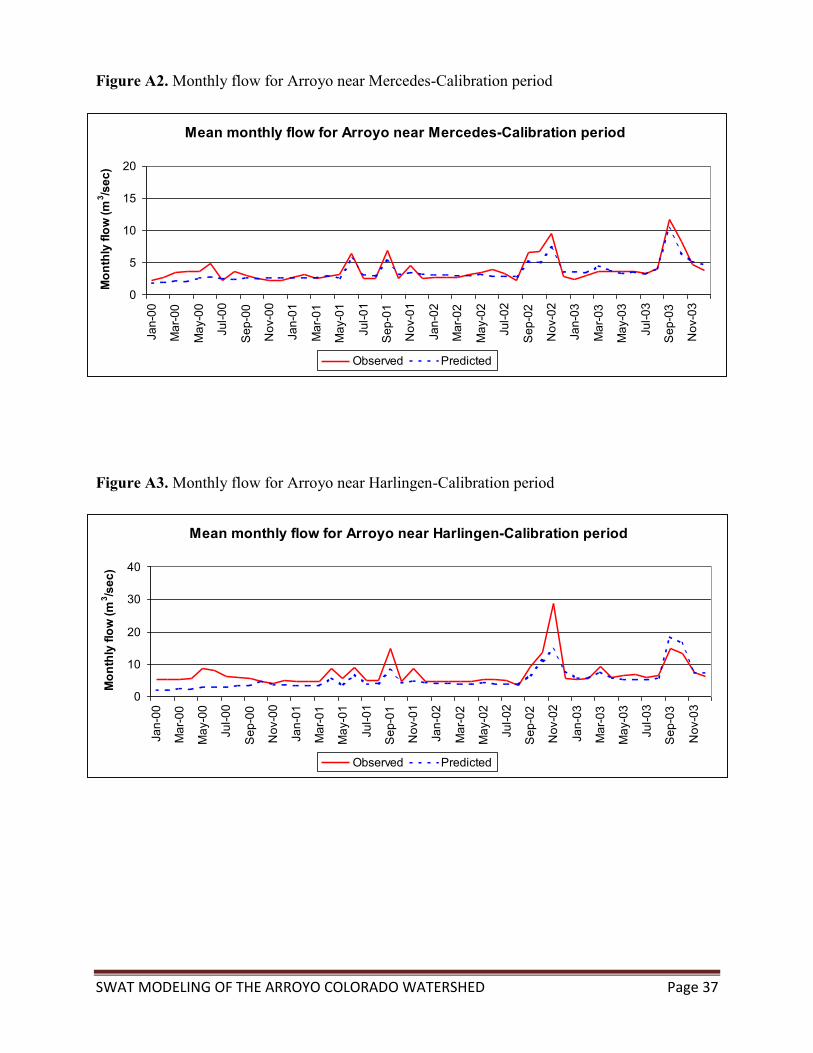
Flow calibration and validation was carried out for two gauges: one near Weslaco/Mercedes and the other
near Harlingen. The model is able to reproduce the flow observations very well in both gauges during
calibration and validation periods (Tables A2 and A3). Similar results were obtained for flow at a daily
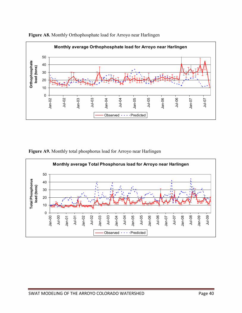
time step. For sediment, the model-predicted values were good when compared to observations except for
a couple of over-estimated peaks. Orthophosphate was predicted well by the model. However, total
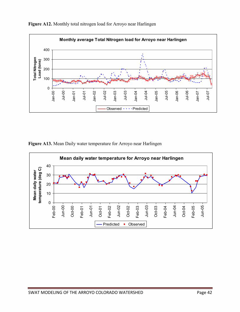
phosphorus was over-estimated. Also, for nitrogen, the model-predicted values were good enough to use
for scenario trials. We did not carry out calibrations for water temperature and dissolved oxygen. SWAT
estimates water temperature as an empirical function of air temperature and therefore, no parameter is
available for calibration. For dissolved oxygen, the model gave better results without any requirement for
calibration. All the calibration and validation results are provided in Figures A2-A14 and tables A1-A7 in
Appendix A.

SWAT MODELING OF THE ARROYO COLORADO WATERSHED Page 24
Watershed scenarios for 2015 and 2025
Estimation of future land cover maps
Data used
The data used includes city limits, census data, population projections, and land use/land cover maps from
multiple years. City limit information was produced by the Texas Department of Transportation
(TxDOT). The Census data was from the 1990 and 2000 census. The population projections were
produced by the Texas Water Development Board based on the 2000 census. Projections from 2010,
2020, and 2030 were averaged to create projections for 2015 and 2025. Three different land use maps
from 1992, 1998, and 2007 were used. The 1992 map was a subset of the National Land Cover Dataset
(NLCD). The 1998 classification was produced by the Texas Commission on Environmental Quality
(TCEQ) and the 2007 Classification was produced by the Spatial Sciences Lab at Texas A&M University
in College Station (SSL).
Method
To quantify land cover change, the three available land cover maps (for years 1992, 1998 and 2007)
needed to be in one format and reclassified into a common scheme. The two vector classifications were
converted to raster using the extent and cell size of the 1998 classification, which had the same extent as
the watershed boundary. After reclassification, pixel counts were exported and converted to acres. The
results were observed in a table with both area and % of watershed values (% of watershed occupied by a
certain land use).
The amount of residential land use areas within each city was extracted using the city limits and each of
the reclassified maps. Cities with populations greater than 500 as of 2000 were identified and extracted.
This was necessary because population projections were not available for cities with populations less than
500. Some did not have a population of 500 in 1990, but did in 2000, so they were included. The trend
would simply include one less value. In some cases the population values did not steadily increase and
there were some slight declines or no growth. This was because the values were extracted from different
sources that were not consistent. If the population declined, it was averaged with the value before and
after the decline to achieve steady growth. Each of the city limits was then given a unique identification
number of 1000 through 21000. This ID number was then used to convert the city limits to raster. It was
necessary to use values of 1000 or greater since the highest class values were three digits long, although
the highest observed in the land use maps were two digits. Additional overlay was then used to extract the
land uses within the city limits. The residential and nonresidential developed land uses were extracted and
the total area of each was calculated individually. These values were then analyzed and used to compute
future residential land use acreage.

SWAT MODELING OF THE ARROYO COLORADO WATERSHED Page 25
In order to map probable locations of development or land use change, previous land use change was
mapped using combination overlays of classifications with the classification from the previous time
period. An overlay was also created using the oldest and most recent classifications. Using combinations
makes it possible to identify areas that have changed from or to a specific land use. In this case, areas that
changed to residential were extracted from combinations of 1992 and 1998, 1998 and 2007, and 1992 and
2007. Using each of the combinations accounted somewhat for the differences in extent between 1998
and 2007, although not entirely. The combinations identified what land uses were most frequently being
developed into residential. Areas where the land use changed to residential as well as potential areas for
residential development would both be used in the production of the final future land cover maps (Table
8).
The results show that rapid urban growth is likely to continue in the watershed through 2015 and 2025.
Each city will experience growth in residential, infrastructure, and industrial land uses. This growth will
require that other land uses decline to accommodate the increase. It also appears that many of the larger
urban areas have little available land within their city limits for further development. To accommodate
further growth, city limits will need to expand into the rural areas. Agricultural and industrial land uses
provide work for the population living in the area so they will likely limit growth to some extent.
However, residential expansion is currently occurring in agricultural lands as well as pastures.
Several assumptions were made about residential and urban expansion. Water and wetlands are unlikely
to be developed although wetlands may expand in some areas due to the expansion of existing wetlands
or the creation of wetlands to help improve water quality near wastewater treatment facilities.
Transportation and infrastructure will expand as structures are built and neighborhoods expand, but this
cannot be predicted with any confidence. Industry and agribusiness were expanded as part of the
infrastructure.

SWAT MODELING OF THE ARROYO COLORADO WATERSHED Page 26
Table 8. Present and estimated future land cover in the watershed
Land Cover
Area in acres
Present 2015 2025
Cultivated (CULT)
Range-Brush (RNGB)
Range-Grasses (RNGE)
Urban-Commercial (UCOM)
Urban-Industrial (UIDU)
Urban-High density residential (URHD)
Urban-Low density residential (URLD)
Urban-Transportation (UTRN)
Open water (WATR)
Wetland-Forested (WETF)
Wetland-Non-forested (WETN)
244,436.3
67,090.0
11,104.9
7,598.1
2,219.4
0.0
37,753.0
5,269.5
25,406.3
14,716.1
2,350.8
228,231.6
63,067.4
10,439.1
12,071.1
4,781.6
707.5
41,743.0
12,576.8
25,386.1
16,589.1
2,350.8
215,670.7
58,040.6
9,615.5
15,008.1
10,567.4
1,061.2
45,870.7
17,681.6
25,465.3
16,612.4
2,350.8
Development of model input files for future scenarios
In this study we attempted to predict land cover conditions of the Arroyo Colorado watershed for 2015
and 2025. Estimated land cover maps were the starting point for future scenario files. Soon after
estimating future land cover, the input file generation for a future scenario goes as follows. The watershed
and subwatershed boundaries are the same as base line. Soil map and slope information are also the same.
However, the land cover map will be different (e.g. for scenario-2015 the land cover map to be used is the
one that is estimated). The procedure used before for discretizing the subwatersheds to HRUs was also
used here. The thresholds used for land cover, soil and slope are kept the same for scenarios as well to
prevent any uncertainties arising from spatial discretization of subwatersheds in the scenarios, which
might interfere the analysis of water quality results. Once the HRUs are delineated for each scenario, the
required input files to run SWAT model are generated this way:
Soon after generating HRUs of scenarios, the procedure starts with base line HRUs that are calibrated for
flow and selected water quality constituents. The HRUs of a scenario (say 2015) is compared with the
HRUs of base line by matching the land cover, soil and slope. This will identify three sets of information.
The HRUs of base line is to be a) kept b) removed and c) created new to represent the scenario
conditions. For those HRUs to be kept, it involves changing the HRU area only. For those HRUs to be
removed either we can fully delete them from the input files or make the HRU area zero. The later is
followed for convenience and automation. The new HRUs to be created can be copied from existing
baseline HRUs by carefully looking for land cover, soil and slope combinations. If a similar HRU does
not exist in a subbasin, then HRUs can be copied from neighboring subbasins. By generating the model

SWAT MODELING OF THE ARROYO COLORADO WATERSHED Page 27
input files this way, we can avoid calibration of scenario files and proceed straight away to analysis of
results.
Analysis of present and future water quality trends
Implementation of BMPs in the watershed, improvement in wastewater treatment, access of wastewater
treatment to more colonia residents, strict effluent standards, treatment of effluent using polishing ponds
and wetlands have improved the quality of water in the Arroyo Colorado over a period of few years. This
is evident from the later part of dissolved oxygen trends (consistently close to 7) observed near Harlingen
(Fig. A14). The improvements in water quality are also visible from the dissolved oxygen trends
estimated from the model and analyzed using binomial method (Table 9). From the table we can see that
most sections of tidal Arroyo Colorado are having DO compliance except at reach 13 and 14. These
reaches are not on the main Arroyo Colorado, but they drain to reach 15 of the Arroyo Colorado.
Nonpoint source transport of nutrients from cultivated fields can be attributed to the DO problem of
reaches 13 and 14. The model estimates a threat to DO in some reaches of nontidal portion of the Arroyo
Colorado (Table 9). Point source discharge (especially from subbasins 2 and 3) can be attributed to the
problem in the nontidal portion of the Arroyo Colorado. It should be noted that any problem in DO due to
point source is long lasting and spreads to other reaches downstream. On the other hand, DO problem
from nonpoint source nutrient pollution is highly seasonal and mostly localized.

SWAT MODELING OF THE ARROYO COLORADO WATERSHED Page 28
Table 9. Modeled dissolved oxygen compliance in various reaches-Binomial Analysis results
(with existing BMPs in the watershed model setup)
Reach
Location
Confidence of Dissolved Oxygen Compliance (%)
[Average number of days/year when DO < 4 mg/L]
Baseline (present) 2015 2025
2
3
4
5
6
7
8
9
10
11
12
Non-tidal
Non-tidal
Non-tidal
Non-tidal
Non-tidal
Non-tidal
Non-tidal
Non-tidal
Non-tidal
Non-tidal
Non-tidal
0.0 [316]#
0.0 [237]#
0.0 [106]#
100.0 [34]
100.0 [34]
100.0 [24]
100.0 [27]
0.0 [45]
100.0 [27]
0.0 [226]#
100.0 [24]
0.0 [342]#
0.0 [273]#
0.0 [145]#
0.0 [56]
96.7 [34]
100.0 [24]
100.0 [27]
0.0 [46]
100.0 [29]
0.0 [250]#
100.0 [26]
0.0 [334]#
0.0 [274]#
0.0 [161]#
0.0 [62]
0.03 [40]
100.0 [28]
100.0 [29]
0.0 [46]
99.9 [33]
0.0 [171]#
100.0 [29]
we
13
14
15
16
17
1
Tidal
Tidal
Tidal
Tidal
Tidal
Tidal
93.0 [37]
85.0 [38]
100.0 [22]
100.0 [31]
100.0 [17]
100.0 [16]
19.0 [38]
0.5 [40]
100.0 [23]
97.8 [34]
100.0 [19]
100.0 [14]
0.0 [44]
0.0 [43]
100.0 [25]
100.0 [32]
100.0 [16]
100.0 [15]
# Model over reacted to point source loads. Therefore, care was taken while interpreting the results and
translating to recommendations
In 2015, because of land cover change and population increase, the water quality is expected to be worse,
which is correctly estimated by the model. Although the trends in DO for 2015 are similar to base line,
the average number of days per year during which DO concentration is less than 4 mg/L is more for 2015
than base line for most reaches (Table 9). It should be noted that the proposed wastewater polishing
ponds, regional wetlands and better emission standards for effluents to the Arroyo Colorado watershed as
described by the watershed protection plan are going to be very helpful to protect the water quality of the
Arroyo Colorado. As a part of this study, we carried out the suite of BMPs required to bring the DO in
compliance . The subbasins of the Arroyo Colorado were prioritized for implementation of BMPs based
on model-predicted average number of days when DO is less than 4 mg/L (Table 10) in the reach. The
BMPs to be implemented in the cultivated area were also prioritized based on the extent of load
reductions they can bring to the Arroyo Colorado (Table 11).

SWAT MODELING OF THE ARROYO COLORADO WATERSHED Page 29
Table 10. Prioritized implementation of BMPs by subbasin in the watershed
Prioritization of BMPs based on
Dissolved Oxygen Total Nitrogen Total Phosphorus
2
3
11
4
9
14
13
5
6
16
10
8
12
7
15
17
1
8
7
5
4
10
12
11
15
6
3
2
9
13
14
16
17
1
8
5
7
6
10
4
11
15
2
9
3
16
13
14
12
17
1
Table 11. Possible load reductions from different BMPs and their prioritization for implementation
Best Management Practice % of load reductions obtained from BMPs in
Total Nitrogen Total Phosphorus Sediment
Residue management
Irrigation BMPs
Nutrient management
Seasonal residue management
Land leveling
Tile drains*
22.05
11.85
4.1
3.25
34.75
6.6
45.1
4.25
19.85
24.15
*
1.7
20.2
3.00
0.25
4.75
42.4
0.8 * Negative results (increase in nutrient loads) possible sometimes. Therefore, care should be taken while
choosing these BMPs.
Not all BMPs are fully effective in controlling nutrient loads or dissolved oxygen in the Arroyo Colorado.
For example, tile drains, when implemented for reducing water table, will transport more soluble nitrogen
to the river than when there are no drains. Also, residue management is much more effective than
seasonal residue management. Therefore, care should be taken while choosing BMPs for implementation
in a subbasin.

SWAT MODELING OF THE ARROYO COLORADO WATERSHED Page 30
Discussion of mitigation of dissolved oxygen problems
Table 12 shows the suite of BMPs required by 2015 to bring DO compliance for the Arroyo Colorado.
The study identified a set of BMPs for different subbasins where they can work better. Irrigation BMPs in
Table 12 is a collection of three different BMPs, namely irrigation water management, irrigation water
conveyance (in the form of) pipeline, and irrigation system-surface surge valves.
Table 12. Suite of additional BMPs needed by 2015 to meet dissolved oxygen criteria
Subbasin
Scenario 2015-Area of different BMPs (acres)
Land leveling Residue
management
Irrigation
BMPs
Nutrient
management
2
3
4
5
9
11
13
14
Total
1,902
682
16,119
8,107
1,757
1,632
489
7,003
37,691
1,902
----
----
9,238
509
7,463
4,374
2,452
25,938
----
----
16,715
----
----
----
489
51
17,254
----
1,460
----
9,315
633
6,099
4,373
1,667
23,549
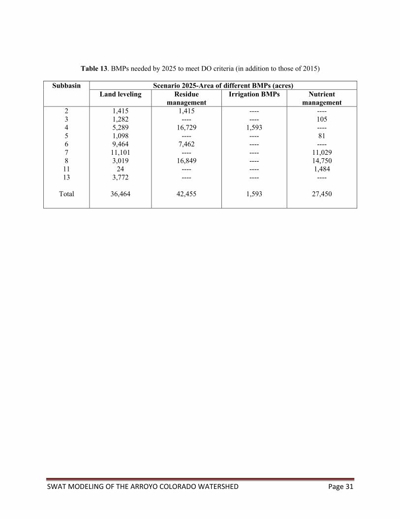
Implementation of additional BMPs can take care of the DO problem in the tidal portion of the Arroyo
Colorado. However, for the nontidal portion of the Arroyo Colorado, implementation of BMPs alone is
insufficient to address the DO problem. An integrated approach of reducing/reusing/better treating of
point source discharge along with implementation of BMPs is needed to address the nontidal DO
problem. This study recommends reducing/reusing/treating at least 40% of pollutants from point sources
associated with subbasins 2, 3, 9, and 11. The same recommendations are suggested for scenario 2025 as
well. However, it is recommended to implement additional BMPs (in addition to whatever suggested for
2015 (see Table 12) in the watershed to take care of nonpoint source transport of nutrients and sediments
from cultivated areas (Table 13).
SWAT MODELING OF THE ARROYO COLORADO WATERSHED Page 31
Table 13. BMPs needed by 2025 to meet DO criteria (in addition to those of 2015)
Subbasin Scenario 2025-Area of different BMPs (acres)
Land leveling Residue
management
Irrigation BMPs Nutrient
management
2
3
4
5
6
7
8
11
13
Total
1,415
1,282
5,289
1,098
9,464
11,101
3,019
24
3,772
36,464
1,415
----
16,729
----
7,462
----
16,849
----
----
42,455
----
----
1,593
----
----
----
----
----
----
1,593
----
105
----
81
----
11,029
14,750
1,484
----
27,450

SWAT MODELING OF THE ARROYO COLORADO WATERSHED Page 32
Acknowledgments
The streamflow data were provided by the International Boundary and Water Commission. Water quality
data were provided by TCEQ. Dr. Roger Miranda of TCEQ provided valuable guidance during the data
collection and model setup. Present and future land cover maps for the watershed were generated under
the guidance of Dr. Raghavan Srinivasan of Spatial Sciences Lab (Texas A&M University) with
assistance from David Shoemate. Ronnie Ramirez and Andy Garza of TSSWCB helped to get data on
land management practices and BMPs adopted by landowners in the watershed. Nina Omani of Spatial
Sciences Lab carried out the flow calibration, and migration of model input files to the most recent
version. Dr. Jeff Arnold and Nancy Sammons of USDA-ARS updated the model source code. Dr. Santhi
Chinnasamy of Texas AgriLife Research provided useful suggestions for this project. Georgie Mitchell
and Dr. Mike White estimated pollutant loads from grab sample water quality observations. Allen
Berthold of Texas Water Resources Institute managed the project. The members of the Arroyo Colorado
Watershed Partnership provided valuable comments and suggestions during the course of the study. Many
thanks go out to all of those who helped to complete this project.

SWAT MODELING OF THE ARROYO COLORADO WATERSHED Page 33
References
Arnold, J.G., Allen, P.M., and Bernhardt, G. (1993). “A comprehensive surface-groundwater
flow model”. Journal of Hydrology, 142, 47–69.
Bean, B. and McFarland, M. 2008 Getting the most out of your nitrogen fertilization in Corn.
Texas AgriLife Extension Service, Texas A&M University System, USA.
Bosch, D.D., Sheridan, J.M., Batten, H.L., and Arnold, J.G. (2004). “Evaluation of the SWAT
model on a coastal plain agricultural watershed”. Transactions of the American Society of
Agricultural Engineers, 47 (5), 1493–1506.
Burt, C.M. (1993). “Irrigation canal simulation model usage”. Journal of Irrigation and
Drainage Engineering, 119 (4), 631–636.
Cruces L. (2003). “Drought strategies for Cotton”. Co-operative Extension Service, Circular
582, College of Agriculture and Home Economics, New Mexico State University.
Fipps, G. (2005). “Potential Water Savings in Irrigated Agriculture for the Rio Grande Planning
Region”, Irrigation Technology Center, Department of Biological and Agricultural
Engineering, Texas A&M University System
Fipps, G., and Pope, C. (1998). “Implementation of a district management system in the
Lower Rio Grande Valley of Texas”. In Proc. 14th Technical Conference on Contemporary
Challenges in Irrigation and Drainage, U.S. Committee on Irrigation and Drainage, Phoenix,
(June 3–6, 1998).
Fipps, G., and Pope, C. (1999). “Irrigation district efficiencies and potential water savings in the
Lower Rio Grande Valley of Texas”, Texas A&M University
Fohrer, N., Haverkamp, S., Eckhardt, K., Frede, H.G. (2001). “Hydrologic response to land use
changes on the catchment scale”. Physics and Chemistry of Earth 26 (7–8), 577–582.
Gassman, P.W., Reyes, M.R., Green, C.H., Arnold, J.G. (2007). “The soil and water assessment
tool: historical development, applications and future research directions”. Transactions of the
American Society of Agricultural and Biological Engineers 50 (4), 1211–1250.
George, B.A., Raghuwanshi, N.S. and Singh. R. (2004). “Development and testing of a GIS
integrated irrigation scheduling model”, Agricultural Water Management, 66, 221–237.
Moriasi, D.N., Arnold, J.G., Van Liew, M.W., Bingner, R.L., Harmel, D., and Veith, R.D.
(2007). “Model evaluation guidelines for systematic quantification of accuracy in watershed
simulations” Transactions of the American Society of Agricultural and Biological Engineers,
50 (3), 885–900.
Nash, J. E., and Suttcliffe, J.V. (1970). “River Flow Forecasting through Conceptual Models,
Part I – A Discussion of Principles”. Journal of Hydrology 10(3): 282–290.
Neitsch, S.L., Arnold, J.G., Kiniry, J.R., and Williams, J.R. (2004). “Soil and Water Assessment
Tool-Version 2000-User’s Manual”, Temple, TX, USA.

SWAT MODELING OF THE ARROYO COLORADO WATERSHED Page 34
Nicolaisen, J.E., Gilley, J.E., Eghball, B. and Marx, D.B. Crop residue effects on runoff nutrient
concentrations following manure application. Transactions of the ASABE, 50(3): 939–944.
Nunez, J., Hartz, T., Suslow, T., Mc Giffen, M.and Natwick, E. 2008. Carrot Production in
California, Vegetable Production Series, University of California Vegetable Research and
Information Center, University of California, USA.(publication 7226)
Obreza, T.A. and Morgan, K.T. 2008 Nutrition of Florida Citrus Trees, Institute of Food and
Agricultural Sciences Extension, University of Florida, USA (SL 253).
Parcher, J. and Humberson, D.G. 2007. CHIPS: A New Way to Monitor Colonias Along the
united States-Mexico Border, U.S. Geological Survey Reston, VA, USA (Open File Report
2007-1230).
Rains, T.H., and Miranda, R.M. (2002). “Simulation of Flow and Water Quality of the Arroyo
Colorado, Texas, 1989-99”. United States Geological Survey-Water Resources Investigations
Report, No: 02-4110.
Rosenthal, W., and Garza, A. (2007). “SWAT Simulations of Nutrient Loadings in the Arroyo
Colorado Watershed”. In Proc. 2007 ASABE Annual International Meeting, Minneapolis,
Minnesota (paper No. 072031).
Santhi, C., and Pundarikanthan, N.V. (2000). “A new planning model for canal scheduling of
rotational irrigation” Agricultural Water Management, 43, 327–343.
Santhi, C., Muttiah, R.S., Arnold, J.G., and Srinivasan, R. (2005). “A GIS based regional
planning tool for irrigation demand assessment and savings using SWAT”, Transactions of
the American Society of Agricultural Engineers, 48(1): 137–147.
Sauls, J.W. 2010 Citrus – Watering, Fertilizing, Weed Control, Pruning and Cold Protection.
Home Fruit Production - Citrus Texas Agricultural Extension Service, Texas Agricultural
Extension Service, Texas A&M University System, Weslaco, Texas (B-1629).
SCS. (1956). “Hydrology. National Engineering Handbook, Supplement A, Section 4”. Soil
Conservation Service, US Department of Agriculture: Washington, DC; Chapter 10.
Stichler, C., and McFarland, M. (2001). “Crop Nutrient Needs in South and Southwest Texas”,
Texas Agricultural Extension Service, Texas A&M University System. (B-6053, 04-01)
Stichler, C., McFarland, M., and Coffman, C. (2008). “Irrigated and Dryland Grain Sorghum
Production South and Southwest Texas”, Texas Agricultural Extension Service, The Texas
A&M University System (5M—5-97, New AGR14).
Surface Water Quality Monitoring Program. 2008. Guidance for Assessing and Reporting
Surface Water Quality in Texas, Texas Commission on Environmental Quality, Austin, TX,
USA.
Texas Water Development Board. 2005 Water Conservation Best Management Practices (BMP)
Guide for Agriculture in Texas. Water Conservation Implementation Task Force (Report
362), Texas Water Development Board, USA.
Trostle, C., and Porter, P. (2001). “Common Concerns in West Texas Sunflower Production

SWAT MODELING OF THE ARROYO COLORADO WATERSHED Page 35
and Ways to Solve Them”, Texas Agricultural Extension Service, The Texas A&M
University System.
United States Environmental Protection Agency (USEPA). 1988. Design Manual-Constructed
Wetlands and Aquatic Plant Systems for Municipal Wastewater Treatment. Center for
Environmental Research Information, Cincinati, OH, USA
Vegetable Team Production. (2008). “Onion Production Guide”, Cooperative Extension Service,
The University of Georgia/College of Agricultural and Environmental Sciences.
“Water Conservation Best Management Practices (BMP) Guide for Agriculture in Texas”, Based
on the Agricultural BMPs contained in: Texas Water Development Board, Report 362, Water
Conservation Implementation Task Force.
Wiedenfeld, B., and Enciso, J. (2008). “Sugarcane Responses to Irrigation and Nitrogen in
Semiarid South Texas”, Agronomy Journal, 100, 665–671.
Wiedenfeld, B., Sauls, J. (2008). “Long term fertilization effects on ‘Rio Red’ grapefruit yield
and shape on a heavy textured calcareous soil”. Scientia Horticulturae, 118, 149–154.

SWAT MODELING OF THE ARROYO COLORADO WATERSHED Page 36
Appendix A
Figure A1. Modeling canal irrigation
HRUs
HRUs with Water
Conveyance
Efficiency
Irrigated?
Critical growth stages-days
after planting, depth,
frequency, timing and number
of irrigations
Crop
Crop fact sheets, Publications
HRU loop
Depth, timing and frequency of
irrigation
Sub basin
Land cover
Soil
Merge
Merge
Internal process in SWAT interface
Irrigation
district
Conveyance
Efficiency
Merge Yes No
Merge Run model without
any irrigation
Water stress
Probable days for
irrigation
Extract
Extract
Merge
Stop
No Yes
Pre-defined process
Pre-defined process
End of
HRUs
SWAT MODELING OF THE ARROYO COLORADO WATERSHED Page 37
Figure A2. Monthly flow for Arroyo near Mercedes-Calibration period
Figure A3. Monthly flow for Arroyo near Harlingen-Calibration period
Mean monthly flow for Arroyo near Mercedes-Calibration period
0
5
10
15
20
Ja
n-0
0
Ma
r-0
0
Ma
y-0
0
Ju
l-0
0
Se
p-0
0
No
v-0
0
Ja
n-0
1
Ma
r-0
1
Ma
y-0
1
Ju
l-0
1
Se
p-0
1
No
v-0
1
Ja
n-0
2
Ma
r-0
2
Ma
y-0
2
Ju
l-0
2
Se
p-0
2
No
v-0
2
Ja
n-0
3
Ma
r-0
3
Ma
y-0
3
Ju
l-0
3
Se
p-0
3
No
v-0
3
Mo
nth
ly f
low
(m
3/s
ec
)
Observed Predicted
Mean monthly flow for Arroyo near Harlingen-Calibration period
0
10
20
30
40
Ja
n-0
0
Ma
r-0
0
Ma
y-0
0
Ju
l-0
0
Se
p-0
0
No
v-0
0
Ja
n-0
1
Ma
r-0
1
Ma
y-0
1
Ju
l-0
1
Se
p-0
1
No
v-0
1
Ja
n-0
2
Ma
r-0
2
Ma
y-0
2
Ju
l-0
2
Se
p-0
2
No
v-0
2
Ja
n-0
3
Ma
r-0
3
Ma
y-0
3
Ju
l-0
3
Se
p-0
3
No
v-0
3
Mo
nth
ly f
low
(m
3/s
ec
)
Observed Predicted

SWAT MODELING OF THE ARROYO COLORADO WATERSHED Page 38
Figure A4. Monthly flow for Arroyo near Mercedes-Validation period
Figure A5. Monthly flow for Arroyo near Harlingen-Validation period
Mean monthly flow for Arroyo near Mercedes-Validation period
0
5
10
15
20Ja
n-0
4
Ma
r-0
4
Ma
y-0
4
Ju
l-0
4
Se
p-0
4
No
v-0
4
Ja
n-0
5
Ma
r-0
5
Ma
y-0
5
Ju
l-0
5
Se
p-0
5
No
v-0
5
Ja
n-0
6
Ma
r-0
6
Ma
y-0
6
Ju
l-0
6
Se
p-0
6
No
v-0
6
Mo
nth
ly f
low
(m
3/s
ec
)
Observed Predicted
Mean monthly flow for Arroyo near Harlingen-Validation period
0
10
20
30
40
Ja
n-0
4
Ma
r-0
4
Ma
y-0
4
Ju
l-0
4
Se
p-0
4
No
v-0
4
Ja
n-0
5
Ma
r-0
5
Ma
y-0
5
Ju
l-0
5
Se
p-0
5
No
v-0
5
Ja
n-0
6
Ma
r-0
6
Ma
y-0
6
Ju
l-0
6
Se
p-0
6
No
v-0
6
Mo
nth
ly f
low
(m
3/s
ec
)
Observed Predicted

SWAT MODELING OF THE ARROYO COLORADO WATERSHED Page 39
Figure A6. Monthly sediment load for Arroyo near Mercedes
Figure A7. Monthly sediment load for Arroyo near Harlingen
Monthly average Sediment load for Arroyo near Mercedes
0
5
10
15
20
25
Ja
n-0
0
Ju
l-0
0
Ja
n-0
1
Ju
l-0
1
Ja
n-0
2
Ju
l-0
2
Ja
n-0
3
Ju
l-0
3
Ja
n-0
4
Ju
l-0
4
Ja
n-0
5
Ju
l-0
5
Ja
n-0
6
Ju
l-0
6
Se
dim
en
t lo
ad
(Th
ou
sa
nd
to
ns
)
Observed Predicted
Monthly average Sediment load for Arroyo near Harlingen
0
20
40
60
80
Ja
n-0
0
Ju
l-0
0
Ja
n-0
1
Ju
l-0
1
Ja
n-0
2
Ju
l-0
2
Ja
n-0
3
Ju
l-0
3
Ja
n-0
4
Ju
l-0
4
Ja
n-0
5
Ju
l-0
5
Ja
n-0
6
Ju
l-0
6
Ja
n-0
7
Ju
l-0
7
Se
dim
en
t lo
ad
(Th
ou
sa
nd
to
ns
)
Observed Predicted
SWAT MODELING OF THE ARROYO COLORADO WATERSHED Page 40
Figure A8. Monthly Orthophosphate load for Arroyo near Harlingen
Figure A9. Monthly total phosphorus load for Arroyo near Harlingen
Monthly average Orthophosphate load for Arroyo near Harlingen
0
10
20
30
40
50
Ja
n-0
2
Ju
l-0
2
Ja
n-0
3
Ju
l-0
3
Ja
n-0
4
Ju
l-0
4
Ja
n-0
5
Ju
l-0
5
Ja
n-0
6
Ju
l-0
6
Ja
n-0
7
Ju
l-0
7
Ort
ho
ph
os
ph
ate
loa
d (
ton
s)
Observed Predicted
Monthly average Total Phosphorus load for Arroyo near Harlingen
0
10
20
30
40
50
Ja
n-0
0
Ju
l-0
0
Ja
n-0
1
Ju
l-0
1
Ja
n-0
2
Ju
l-0
2
Ja
n-0
3
Ju
l-0
3
Ja
n-0
4
Ju
l-0
4
Ja
n-0
5
Ju
l-0
5
Ja
n-0
6
Ju
l-0
6
Ja
n-0
7
Ju
l-0
7
Ja
n-0
8
Ju
l-0
8
Ja
n-0
9
Ju
l-0
9
To
tal P
ho
sp
ho
rus
loa
d (
ton
s)
Observed Predicted

SWAT MODELING OF THE ARROYO COLORADO WATERSHED Page 41
Figure A10. Monthly ammonia nitrogen load for Arroyo near Mercedes
Figure A11. Monthly nitrate nitrogen load for Arroyo near Harlingen
Monthly average Ammonia Nitrogen load for Arroyo near Mercedes
0
5
10
15
20Ja
n-0
0
Ju
l-0
0
Ja
n-0
1
Ju
l-0
1
Ja
n-0
2
Ju
l-0
2
Ja
n-0
3
Ju
l-0
3
Ja
n-0
4
Ju
l-0
4
Ja
n-0
5
Ju
l-0
5
Ja
n-0
6
Ju
l-0
6
Ja
n-0
7
Ju
l-0
7
Ja
n-0
8
Ju
l-0
8
Ja
n-0
9
Ju
l-0
9
Am
mo
nia
Nit
rog
en
Lo
ad
(to
ns
)
Observed Predicted
Monthly average Nitrate Nitrogen load for Arroyo near Harlingen
0
100
200
300
400
Ja
n-0
2
Ju
l-0
2
Ja
n-0
3
Ju
l-0
3
Ja
n-0
4
Ju
l-0
4
Ja
n-0
5
Ju
l-0
5
Ja
n-0
6
Ju
l-0
6
Ja
n-0
7
Ju
l-0
7
Nit
rate
Nit
rog
en
Lo
ad
(to
ns
)
Observed Predicted
SWAT MODELING OF THE ARROYO COLORADO WATERSHED Page 42
Figure A12. Monthly total nitrogen load for Arroyo near Harlingen
Figure A13. Mean Daily water temperature for Arroyo near Harlingen
Monthly average Total Nitrogen load for Arroyo near Harlingen
0
100
200
300
400Ja
n-0
0
Ju
l-0
0
Ja
n-0
1
Ju
l-0
1
Ja
n-0
2
Ju
l-0
2
Ja
n-0
3
Ju
l-0
3
Ja
n-0
4
Ju
l-0
4
Ja
n-0
5
Ju
l-0
5
Ja
n-0
6
Ju
l-0
6
Ja
n-0
7
Ju
l-0
7
To
tal N
itro
ge
n
Lo
ad
(to
ns
)
Observed Predicted
Mean daily water temperature for Arroyo near Harlingen
0
10
20
30
40
Fe
b-0
0
Ju
n-0
0
Oct-
00
Fe
b-0
1
Ju
n-0
1
Oct-
01
Fe
b-0
2
Ju
n-0
2
Oct-
02
Fe
b-0
3
Ju
n-0
3
Oct-
03
Fe
b-0
4
Ju
n-0
4
Oct-
04
Fe
b-0
5
Ju
n-0
5
Me
an
da
ily
wa
ter
tem
pe
ratu
re (
de
g C
)
Predicted Observed

SWAT MODELING OF THE ARROYO COLORADO WATERSHED Page 43
Figure A14. Mean daily dissolved oxygen for Arroyo near Harlingen
Mean daily dissolved Oxygen for Arroyo near Harlingen
0
5
10
15
20
Fe
b-0
0
Au
g-0
0
Fe
b-0
1
Au
g-0
1
Fe
b-0
2
Au
g-0
2
Fe
b-0
3
Au
g-0
3
Fe
b-0
4
Au
g-0
4
Fe
b-0
5
Au
g-0
5
Fe
b-0
6
Au
g-0
6
Fe
b-0
7
Au
g-0
7
Fe
b-0
8
Au
g-0
8
Fe
b-0
9
Me
an
da
ily
DO
co
nc
(m
g/L
)
Predicted Observed

SWAT MODELING OF THE ARROYO COLORADO WATERSHED Page 44
Figure A15. Pollutant load from different sources in the watershed model setup
39%
61%
Total Phosphorus
Non-point source Point source
Total Nitrogen
84%
16%
Non-point source Point source
Sediment
99%
1%
Non-point source Point source

SWAT MODELING OF THE ARROYO COLORADO WATERSHED Page 45
Table A1. Model parameters and their range considered for flow calibration
Parameter Definition
Units Spatial
scale
Range of values
Min. Max.
SURLAG
AWC
CN2
EPCO
ESCO
GW_DELAY
GW_REVAP
GWQMN
Surface runoff lag coefficient
Available water capacity
SCS runoff curve number for moisture condition II
Plant uptake compensation factor
Soil evaporation compensation factor
Delay time for aquifer recharge
Groundwater revap coefficient
Threshold water level in shallow aquifer for base flow
days
--
--
--
--
days
--
mm
watershed
HRU
HRU
HRU
HRU
HRU
HRU
HRU
0.001
-0.04
-4.0
0.001
0.001
0.001
0.02
0.01
15
+0.04
+4.0
1
1
100
0.2
100
Table A2. Mean monthly flow results for Arroyo Colorado
Monitoring station Calibration period (2000-2003) Validation Period (2004-2006)
Predicted (m3/sec) Observed (m
3/sec) Predicted (m
3/sec) Observed (m
3/sec)
Near Mercedes
Near Harlingen
3.47
5.24
3.76
6.89
3.79
5.81
5.08
8.20
Table A3. Model performance evaluation for flow calibration
Monitoring station
Calibration period (2000-2003) Validation Period (2004-2006)
R2 Nash and Sutcliffe Efficiency (%) R
2 Nash and Sutcliffe Efficiency (%)
Near Mercedes
Near Harlingen
0.83
0.59
78.6
43.1
0.47
0.41
19.5
1.82
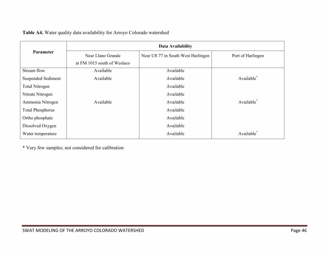
SWAT MODELING OF THE ARROYO COLORADO WATERSHED Page 46
Table A4. Water quality data availability for Arroyo Colorado watershed
Parameter
Data Availability
Near Llano Grande
at FM 1015 south of Weslaco
Near US 77 in South West Harlingen Port of Harlingen
Stream flow
Suspended Sediment
Total Nitrogen
Nitrate Nitrogen
Ammonia Nitrogen
Total Phosphorus
Ortho phosphate
Dissolved Oxygen
Water temperature
Available
Available
Available
Available
Available
Available
Available
Available
Available
Available
Available
Available
Available*
Available*
Available*
* Very few samples; not considered for calibration

SWAT MODELING OF THE ARROYO COLORADO WATERSHED Page 47
Table A5. Model parameters and their range considered for sediment calibration
Parameter Definition
Units Spatial
scale
Range of values
Min. Max.
ADJ_PKR
PRF
SPCON
SPEXP
CH_N2
CH_COV1
CH_COV2
CH_N1
Erosion K
LAT_SED
Flow peak rate adjustment factor for sediment routing in tributaries
Flow peak rate adjustment factor for sediment routing in main channel
Linear parameter controlling sediment re-entrained in channels
An exponent controlling sediment re-entrained in channels
Manning's n value for the main channel
Channel erodibility factor
Channel cover factor
Manning's n value for the tributary channels
Soil erodibility factor
Sediment concentration in lateral flow
--
--
--
--
--
--
--
--
--
mg/L
watershed
watershed
watershed
watershed
reach
reach
reach
subbasin
HRU
HRU
0.0
0.0
0.0001
1.0
0.016
0.0
0.0
0.025
0.0
0.0
1.0
1.0
0.01
2.0
0.15
1.0
1.0
0.15
1.0
--

SWAT MODELING OF THE ARROYO COLORADO WATERSHED Page 48
Table A6. Model parameters and their range considered for nutrient calibration
Parameter Definition
Units Spatial
scale
Range of values
Min. Max.
N_UPDIS
P_UPDIS
NPERCO
PPERCO
PHOSKD
PSP
RS2
RS3
RS4
RS5
BC1
BC2
BC3
BC4
GWSOLP
HLIFE_NGW
Nitrogen uptake distribution parameter
Phosphorus uptake distribution parameter
Nitrogen percolation coefficient
Phosphorus percolation coefficient
Phosphorus soil partitioning coefficient
Phosphorous sorption coefficient
Benthic source rate for dissolved phosphorus
Benthic source rate for ammonia nitrogen
Rate coefficient for organic nitrogen settling
Rate coefficient for organic phosphorus settling
Rate constant for biological oxidation of ammonia to nitrite
Rate constant for biological oxidation of nitrite to nitrate
Rate constant for hydrolysis of organic nitrogen to ammonia
Rate constant for mineralization of organic phosphorus
Concentration of soluble phosphorus in groundwater
Half life of nitrate in the shallow aquifer
--
--
--
--
--
--
--
--
--
--
--
--
--
--
mg/L
days
watershed
watershed
watershed
watershed
watershed
watershed
reach
reach
reach
reach
reach
reach
reach
reach
HRU
HRU
0.0
0.0
0.01
10.0
0.01
0.0
0.001
0.001
0.001
0.001
0.1
0.2
0.2
0.01
0.01
30.0
40
40
1.0
17.5
300
1.0
0.1
0.1
0.1
0.1
1.0
2.0
0.4
0.7
1.0
200

SWAT MODELING OF THE ARROYO COLORADO WATERSHED Page 49
Table A7. Comparison of predicted and observed mean of various water quality parameters
Average parameter values
Near Llano Grande
at FM 1015 south of Weslaco
Near US 77 in South West Harlingen
Predictions Observations Predictions Observations
Suspended sediment load (tons/year)
Ammonia Nitrogen (tons/year)
Nitrate Nitrogen (kg/day)
Total Nitrogen (kg/day)
Ortho Phosphorus (kg/day)
Total Phosphorus (kg/day)
Water temperature ( C)
Dissolved Oxygen (mg/L)
2,634.1
1.3
1,795.0
4.2
8,434.0
--
116.0
107.0
19.8
21.4
24.6
7.2
5,956.0
--
69.0
89.0
21.8
13.5
25.3
7.5
Recommended