Economic Impacts on New Jersey of Upgrading PSE&G’s
Susquehanna-Roseland Transmission System
Dr. Joseph J. Seneca
Dr. Michael L. Lahr
Dr. James W. Hughes
Will Irving
May 2009

Table of Contents
EXECUTIVE SUMMARY ........................................................................................................ i
INTRODUCTION................................................................................................................... 1
Project Background...................................................................................................... 1
Analytical Approach..................................................................................................... 1
Organization of the Report .......................................................................................... 2
ECONOMIC IMPACT ANALYSIS .......................................................................................... 3
Expenditures Considered in the Analysis................................................................... 3
R/ECON™ Input-Output Model................................................................................. 3
Transmission Line and Towers (Monopole Structures)............................................ 4
Expenditure Assumptions ............................................................................................ 4
Economic Impacts ....................................................................................................... 6
Transmission Line and Towers (Lattice Structures)............................................... 11
Expenditure Assumptions .......................................................................................... 11
Economic Impacts ..................................................................................................... 13
East Hanover/Roseland Switching Station............................................................... 17
Expenditure Assumptions .......................................................................................... 17
Economic Impacts ..................................................................................................... 18
Jefferson Switching Station........................................................................................ 22
Expenditure Assumptions .......................................................................................... 22
Economic Impacts ..................................................................................................... 23
Combined Economic Impacts (Monopole Towers).................................................. 27
Combined Economic Impacts (Lattice Towers)....................................................... 30
CONCLUSION .................................................................................................................... 33
APPENDIX A: ECONOMIC AND DEMOGRAPHIC PROFILES AND DYNAMICS.................... 34
APPENDIX B: INPUT-OUTPUT ANALYSIS ......................................................................... 53
APPENDIX C: ECONOMIC IMPACTS OF COMBINED LATTICE-MONOPOLE SCENARIO... 74
i
EXECUTIVE SUMMARY
This report presents the estimated economic impacts in New Jersey of the
approximately $649 - $750 million in expenditures required for construction of the New
Jersey portion of the proposed upgrade to PSE&G’s Susquehanna-Roseland
Transmission Network. The economic impacts estimated are only those associated with
the expenditures to be made on construction of the network upgrade, and do not reflect
any of the potential ongoing economic impacts of the increased transmission capacity
once the upgrade is complete.
The proposed upgrade would add 500 kV of additional power transmission
capacity to the existing 230 kV network. This analysis examines the economic impacts
of the construction of two switching stations and of the transmission line and towers
required to accommodate the increased transmission capacity. Alternative scenarios are
presented to reflect the two different types of tower structures that may be used. If all
249 towers were lattice structures, the estimated total expenditures for the project would
be approximately $649 million, whereas if all the towers were monopole structures, the
estimated expenditures would total $750 million. (Appendix C at the end of the report
provides the aggregate expenditures and economic impacts for a 50%-50% split between
the two types of towers.)
The estimated economic impacts include both direct impacts and indirect impacts.
Direct impacts are those directly associated with the project expenditures, such as the
construction employment required for the project and purchases of material to be used in
construction of the switching station and towers. Indirect impacts are those generated by
the multiplier effects of the initial expenditures, as the salaries paid to workers and the
business revenue generated by the expenditures made on materials in New Jersey are then
re-spent throughout the economy, generating further economic activity and impacts in the
form of employment, gross domestic product, compensation (income) and tax revenues.
Based on the two expenditure scenarios associated with the different types of
towers and on the associated range of project expenditures to be made in New Jersey, the
following economic impacts were estimated:

ii
• Employment. It is estimated that construction of the switching stations and
transmission line and towers will generate from 3,415 to 3,931 total job-years
(one job-year is equal to one job lasting one year). This includes from 2,258 to
2,646 direct job-years, including construction employment, as well as design
work, consulting services and other
• Gross Domestic Product. It is estimated that the construction of the upgrade will
generate between $396.1 and $428.1 million in gross domestic product for New
Jersey.
• Compensation. It is estimated that the total compensation generated by both the
direct and the indirect employment generated by the construction of the upgraded
network will be between $307.5 million and $333.8 million.
• State Tax Revenues. It is estimated that the construction phase of the project will
generate between $8 and $9 million in state taxes.
• Local Tax Revenues. It is estimated that the construction phase of the project will
generate between $7.9 and $9.9 million in local taxes.
1
INTRODUCTION
This report presents the findings of an economic impact analysis of the
approximately $649-$750 million in expenditures required for construction of the New
Jersey portion of the proposed upgrade to PSE&G’s Susquehanna-Roseland
Transmission Network.
Project Background
PJM Interconnection, the regional authority overseeing electricity transmission in
all or part of 13 states, including New Jersey and Pennsylvania, has determined that the
existing 230 kV capacity of the transmission line running from Susquehanna,
Pennsylvania to Roseland, New Jersey is not sufficient to accommodate projected
demand growth in coming years. As a result, PJM has directed PSE&G of New Jersey
and PPL of Pennsylvania to upgrade the network by adding a new 500 kV capacity
transmission line to the existing network. The upgrade will require not only the addition
of the new power line itself, but also construction of new towers to accommodate both
the new 500 kV, as well as the existing 230 kV line, and the construction of two new
switching stations along the transmission route, one in Jefferson, New Jersey and one
near the line’s terminus in Roseland, New Jersey. This economic impact analysis covers
the estimated $649-$750 million of expenditures required for construction of the New
Jersey portion of the new line, including the two switching stations to be built in New
Jersey.
Analytical Approach
The economic impacts of the construction of the new transmission line in New
Jersey are estimated using the R/ECON™ Input-Output model developed and maintained
by the Center for Urban Policy Research at Rutgers University’s Edward J. Bloustein
School of Planning and Public Policy. The model provides estimates of a broad and
detailed range of economic impacts, including employment, gross domestic product,
income and tax revenues. A detailed description of the model and its methodology is
provided with the analysis.

2
The construction of each component of the new transmission infrastructure is
analyzed individually. That is, the transmission line and towers are analyzed separately,
as are each of the two switching stations. In addition, two separate analyses of the
transmission line and tower infrastructure are provided. Because the existing towers
currently carrying the 230 kV line do not meet the specifications required to handle two
lines of the given capacities discussed, an additional 249 new towers are required in New
Jersey. Some of these towers will be monopole structures (i.e., a single pole with
branches holding the transmission lines), while others will be wider lattice-type
structures. Because each of these tower types requires a different mix of material and
labor inputs, two separate analyses are provided, one assuming that all towers are
monopole, and the other assuming that all towers are lattice.
Organization of the Report
The report begins with a brief overview of the expenditures considered in the
analysis. This is followed by a description of the R/ECON™ Input-Output Model and its
application. Next, the analyses of the separate components of the transmission network
are presented. These analyses consist of the all-monopole transmission line and towers,
the all-lattice transmission line and towers, the Jefferson Switching Station, and the
Roseland/East Hanover Switching Station. Each analysis consists of a review of the
input expenditures used in the R/ECON™ Input-Output Model and a detailed
presentation of the estimated economic impacts of those expenditures. A final section
presents the combined impacts of the total investment in New Jersey for both the all-
monopole and all-lattice tower scenarios. This is followed by a brief summary and
conclusions. An appendix presents a brief economic profile of the areas in New Jersey
where the new transmission line would be built.
3
ECONOMIC IMPACT ANALYSIS
Expenditures Considered in the Analysis
Because of the highly specialized nature of the power transmission materials and
equipment needed for construction of the upgraded network, almost all the required
material will be purchased outside of New Jersey. As such, the majority of the impacts
measured in this analysis are generated via the employment of construction workers and
the purchase of specialized services associated with the project. The majority of these
workers and services are expected to come from New Jersey. Detailed explanations of
the specific expenditures made in New Jersey are provided for each component of the
analysis.
R/ECON™ Input-Output Model
The R/ECON™ Input-Output Model at the Center for Urban Policy Research at
the Bloustein School of Planning and Public Policy was used to measure the economic
impacts of the proposed expenditures for the Susquehanna-Roseland network upgrade.
The R/ECON™ model consists of 515 individual sectors of the New Jersey economy and
measures the effect of changes in expenditures in one industry on economic activity in all
other industries. Thus, the expenditures made on labor, materials, legal and design
services, and other inputs for the transmission line have both direct economic effects as
those expenditures become incomes and revenues for workers and businesses, and
subsequent indirect effects as those workers and businesses, in turn, spend those dollars
on other things – consumer goods, business investment expenditures, which, in turn,
become income for other workers and businesses. This income gets further spent, and so
on.
In summary, the R/ECON™ Input-Output model estimates both the direct
economic effects of the initial expenditures (in terms of jobs and income) and the indirect
(or multiplier) effects (in additional jobs and income) of the subsequent economic activity
that occurs following the initial expenditures. The model also estimates the gross
domestic product for New Jersey and the tax revenues generated by the combined direct
and indirect new economic activity caused by the initial spending.
4
Transmission Line and Towers (Monopole Structures)
Expenditure Assumptions
This estimate of the economic impacts for construction of the transmission line
and towers for the Susquehanna-Roseland network assumes that all towers are monopole
structures.1 In order to reflect the full scope of the expenditures included in PSE&G’s
cost estimates for construction of the transmission line and towers portion of the
upgraded network, it was necessary to make several assumptions and adjustments to the
various expenditure items included in PSE&G’s initial cost estimates. Following is an
explanation of this process.
PSE&G’s estimated total cost for construction of the transmission line and
monopole towers is $497.9 million.
The base cost of construction estimated by PSE&G for the all-monopole
transmission line and towers, including labor, materials, third party
professional services and PSE&G support, was $380.4 million, with an
additional 11% in estimated inflation costs (“escalation”) and an
additional 20% in contingency.
In order to incorporate all potential expenditures into the analysis, the
escalation (11%) and contingency (20%) estimates were distributed
proportionately between the costs of labor and material and the other
costs (professional services, PSE&G support, etc.) according to their
respective shares of the $380.4 million base cost.
In addition, the OH&P on labor (25% of base labor and material costs) and
material (10% of base labor and material costs), the Scope Modifications
on labor (15% of base labor and material costs) and material (15% of base
1 Scenarios assuming all monopole and all lattice tower structures are presented in the body of the report. A spreadsheet indicating the aggregate impacts of using 50% of each type of tower structure is presented in Appendix C.
5
labor and material costs), and the Inefficiencies on labor (18% of base
labor and material costs) were also distributed proportionately across the
labor and material components of the base construction cost structure.
The separate expenditures on labor and materials for the laying of tower
foundations were not broken out in PSE&G’s cost specifications. For
purposes of the analysis, 65% of the $59.4 million in expenditures on
foundations was allocated to labor, and the remaining 35% to material.
These various adjustments resulted in total allocations of $247.8 million
for transmission line construction labor and $171.9 million for material.
All direct construction labor was assumed to come from North Jersey.
All specialty materials (conductors, insulators, field wire, tower structures,
etc.) are assumed to be purchased from outside of New Jersey. As such, of
the material expenditures, only the concrete and other material used for
construction of the tower foundations was incorporated into the impact
estimate.
Of the “Other Costs” (i.e., professional services, PSE&G support, etc.)
associated with construction of the transmission line, the costs for
consulting services provided by Louis Berger, the cost of soil borings, the
costs of appraisals, title and mapping costs, and the costs of PSE&G legal
fees were incorporated into the economic impact estimate. These
expenditures totaled approximately $8 million.
In addition, PSE&G’s support costs were allocated according to the shares
reflected in the itemized cost breakdowns of PSE&G support in the cost
estimates for the two switching stations. All of these costs were
incorporated into the economic impact estimate, with the exception of
6
“Licensing/Permits/Bonds/Builder’s Risk.” Of this last category,
approximately $3.8 million in builder’s risk insurance was incorporated
into the expenditure estimates.
As a result of these assumptions and adjustments, $337.5 million of the
total $497.9 million estimate for construction of the transmission line and
towers (or 67.8%) was allocated to expenditures on labor, material and
services in New Jersey.
Economic Impacts
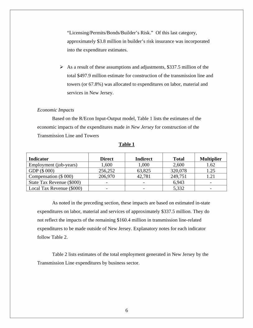
Based on the R/Econ Input-Output model, Table 1 lists the estimates of the
economic impacts of the expenditures made in New Jersey for construction of the
Transmission Line and Towers
Table 1
Indicator Direct Indirect Total Multiplier Employment (job-years) 1,600 1,000 2,600 1.62 GDP ($ 000) 256,252 63,825 320,078 1.25Compensation ($ 000) 206,970 42,781 249,751 1.21 State Tax Revenue ($000) - - 6,943 - Local Tax Revenue ($000) - - 5,332 -
As noted in the preceding section, these impacts are based on estimated in-state
expenditures on labor, material and services of approximately $337.5 million. They do
not reflect the impacts of the remaining $160.4 million in transmission line-related
expenditures to be made outside of New Jersey. Explanatory notes for each indicator
follow Table 2.
Table 2 lists estimates of the total employment generated in New Jersey by the
Transmission Line expenditures by business sector.

7
Table 2
Sector Employment (job-years)
Natural Resources & Mining 16 Construction 1,185 Manufacturing 306 Transportation & Public Utilities 83 Wholesale Trade 101 Retail Trade 276 Financial Activities 159 Services 472 Government 2 Total 2,600
Indicator Explanations:
• Employment
Employment impacts are measured in job-years (i.e., one job lasting one year).
The all-monopole transmission line and towers component of the project is
estimated to generate a total of 2,600 jobs in New Jersey. Based on salary and
benefit estimates for the employment required to upgrade the transmission line,
approximately 1,185 direct construction jobs are estimated to be created. Note
also from Table 1 that the direct employment associated with the construction of
the transmission line (1,600 jobs) exceeds the total construction employment
(1,185 jobs) listed in Table 2. The additional direct employment (415 jobs)
associated with the project is generated in the New Jersey-based wholesale and
manufacturing sectors that produce and distribute the non-specialized materials
used in laying foundations, building access roads, etc., as well as the various
PSE&G internal functions associated with project management and support, and
outside services (e.g., legal) provided by New Jersey firms. Significant additional
indirect employment (1,000 jobs, Table 1) is generated across various sectors,
including services, financial activities, and retail trade.
8
• GDP
Note that the total GDP generated in the state ($320.1 million, Table 1) is close to
the total expenditures estimated for New Jersey. By explicitly excluding those
material expenditures that are to be made outside of New Jersey, the model
minimizes the economic “leakage” that would normally be reflected were they to
have been included. That is, were the excluded $160.4 million in expenditures to
be included, the relative proportion of impacts leaked from the New Jersey
economy would be higher. This leakage is reflected in the per-million dollar
impacts reported below.
• Compensation
Compensation represents the total wages, salaries and supplements to wages and
salaries (i.e., employer contributions to government and private pension funds)
paid for all direct and indirect jobs generated as a result of the project
expenditures made in New Jersey. The transmission line and monopole towers
component is estimated to generate $249.8 million in compensation in New
Jersey.
• State Tax Revenues
State tax revenues are comprised of the income taxes associated with the salaries
paid to the workers in the direct and indirect jobs associated with the project, and
with the sales associated with the economic output generated by the project. The
transmission line and monopole towers component is estimated to generate $6.9
million in state tax revenues.
• Local Tax Revenues
The estimates of the increase in local tax revenues are for the entire state. The
increase represents a long-run estimate of property tax revenues generated by
payment of residential and commercial property taxes from the personal and
business incomes generated by the project and/or resulting from improvements

9
made to property caused by the increased economic activity generated by the
project.
Local tax revenues increase because the additional economic activity from the
transmission line project generates income for workers and revenues for
business2. The increases in personal incomes and in business revenues are, in
part, used to pay property taxes and to improve properties (both residential and
commercial). Thus, households benefitting from the additional jobs and resulting
incomes acquire and/or improve residential properties, and are able to pay rents
and mortgages and the associated property taxes. Similarly, business income and
profits also increase as a direct result of higher sales and output caused by the
project. Businesses subsequently acquire and/or improve their properties.
Historical New Jersey fiscal and economic data are used to measure the
relationship between business revenues and the amount of commercial property
tax revenues collected, and between household incomes and the amount of
residential property tax revenues collected.3 Given the increases in both
household income and the business revenues caused by the expenditures made on
the transmission line, the R/ECON™ Input-Output Model invokes the known
statistical relation of local property tax revenues to both household income and
business revenues in order to estimate the addition to local tax revenues
attributable to the transmission line project.
It is important to note that this additional tax revenue occurs over a period of time.
It is not an immediately generated impact. The economic sequence is as follows.
The additions/improvements to residential and commercial property financed by
the higher household incomes and higher business revenues are, in time, captured
by higher property assessments, which, in turn, generate higher local tax
2 For businesses, the revenue increase is measured in terms of value-added, and it is the change in value-added in the business sector that is the basis for the estimated change in property tax revenues. 3 For the entire state, approximately 76% of total local property tax revenues are attributable to residential property; with approximately 21% derived primarily from commercial and industrial property.

10
revenues. There are time lags between the increase in incomes and revenues, the
improvements to property, and the increase in assessed values. Thus, the local
tax revenue impacts estimated in this analysis are the outcome of a long-run
adjustment process. This process occurs over the entire state based on the
geographical dispersal within New Jersey of the households and businesses that
benefit from the expenditures on the transmission line.
Table 3 provides the per-million dollar spending impacts for the transmission
line. Note that these impacts are calculated per million dollars of total transmission line
expenditures – that is, on the basis of the $497.9 million to be spent both inside and
outside of New Jersey.
Table 3
Indicator Impacts per $1 million of total project expenditures
Employment (job-years) 5.2 GDP $642,864 Income $501,616 State Tax Revenues $13,944 Local Tax Revenues $10,709
11
Transmission Line and Towers (Lattice Structures)
Expenditure Assumptions
This estimate of the economic impacts for construction of the transmission line
and towers for the Susquehanna-Roseland network assumes that all towers are lattice
structures. In order to reflect the full scope of the expenditures included in PSE&G’s cost
estimates for construction of the transmission line and towers portion of the upgraded
network, it was necessary to make several assumptions and adjustments to the various
expenditure items included in PSE&G’s initial cost estimates. Following is an
explanation of this process.
PSE&G’s estimated total cost for construction of the transmission line and
lattice towers is $397.1 million.
The base cost of construction estimated by PSE&G for the all-lattice
transmission line and towers, including labor, materials, third party
professional services and PSE&G support, was $303.2 million, with an
additional 11% in estimated inflation costs (“escalation”) and an
additional 20% in contingency.
In order to incorporate all potential expenditures into the analysis, the
escalation (11%) and contingency (20%) estimates were distributed
proportionately between the costs of labor and material and the other
costs (professional services, PSE&G support, etc.) according to their
respective shares of the $303.2 million base cost.
In addition, the OH&P on labor (25% of base labor and material costs) and
material (10% of base labor and material costs), the Scope Modifications
on labor (15% of base labor and material costs) and material (15% of base
labor and material costs), and the Inefficiencies on labor (18% of base
labor and material costs) were also distributed proportionately across the
labor and material components of the base construction cost structure.
12
The separate expenditures on labor and materials for the laying of tower
foundations were not disaggregated in PSE&G’s cost specifications. For
purposes of the analysis, 65% of the $20.2 million in expenditures on
foundations was allocated to labor, and the remaining 35% to material.
These various adjustments resulted in total allocations of $239.2 million
for transmission line construction labor and $74.4 million for material.
All direct construction labor was assumed to come from North Jersey.
All specialty materials (conductors, insulators, field wire, tower structures,
etc.) are assumed to be purchased from outside of New Jersey. As such, of
the material expenditures, only the concrete and other material used for
construction of the tower foundations was incorporated into the impact
estimate.
Of the “Other Costs” (i.e., professional services, PSE&G support, etc.)
associated with construction of the transmission line, the costs for
consulting services provided by Louis Berger, the cost of soil borings, the
costs of appraisals, title and mapping costs, and the costs of PSE&G legal
fees were incorporated into the economic impact estimate. These
expenditures totaled approximately $8.1 million.
In addition, PSE&G’s support costs were allocated according to the shares
reflected in the itemized cost breakdowns of PSE&G support in the cost
estimates for the two switching stations. All of these costs were
incorporated into the economic impact estimate, with the exception of
“Licensing/Permits/Bonds/Builder’s Risk.” Of this last category,
approximately $3.1 million in builder’s risk insurance was incorporated
into the expenditure estimates.
13
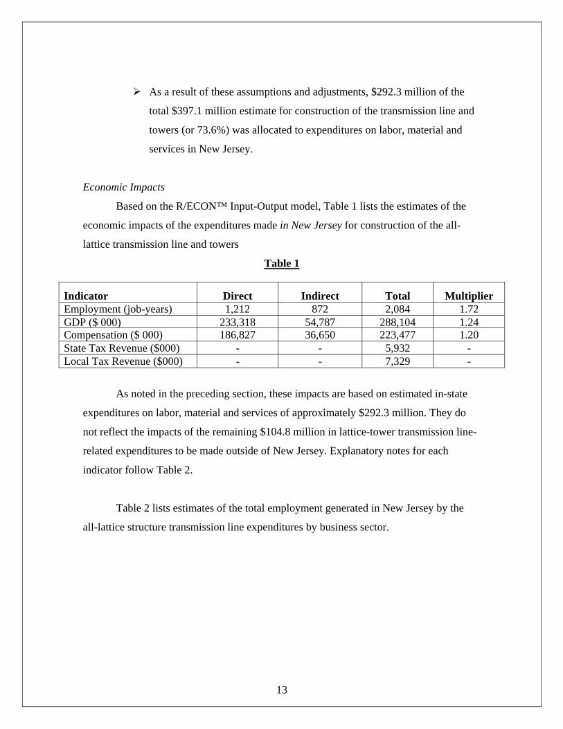
As a result of these assumptions and adjustments, $292.3 million of the
total $397.1 million estimate for construction of the transmission line and
towers (or 73.6%) was allocated to expenditures on labor, material and
services in New Jersey.
Economic Impacts
Based on the R/ECON™ Input-Output model, Table 1 lists the estimates of the
economic impacts of the expenditures made in New Jersey for construction of the all-
lattice transmission line and towers
Table 1
Indicator Direct Indirect Total Multiplier Employment (job-years) 1,212 872 2,084 1.72 GDP ($ 000) 233,318 54,787 288,104 1.24Compensation ($ 000) 186,827 36,650 223,477 1.20 State Tax Revenue ($000) - - 5,932 - Local Tax Revenue ($000) - - 7,329 -
As noted in the preceding section, these impacts are based on estimated in-state
expenditures on labor, material and services of approximately $292.3 million. They do
not reflect the impacts of the remaining $104.8 million in lattice-tower transmission line-
related expenditures to be made outside of New Jersey. Explanatory notes for each
indicator follow Table 2.
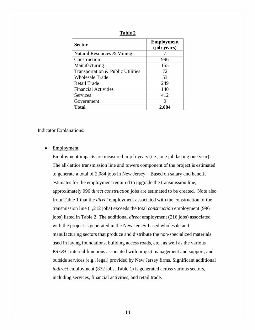
Table 2 lists estimates of the total employment generated in New Jersey by the
all-lattice structure transmission line expenditures by business sector.
14
Table 2
Sector Employment (job-years)
Natural Resources & Mining 7 Construction 996 Manufacturing 155 Transportation & Public Utilities 72 Wholesale Trade 53 Retail Trade 249 Financial Activities 140 Services 412 Government 0 Total 2,084
Indicator Explanations:
• Employment
Employment impacts are measured in job-years (i.e., one job lasting one year).
The all-lattice transmission line and towers component of the project is estimated
to generate a total of 2,084 jobs in New Jersey. Based on salary and benefit
estimates for the employment required to upgrade the transmission line,
approximately 996 direct construction jobs are estimated to be created. Note also
from Table 1 that the direct employment associated with the construction of the
transmission line (1,212 jobs) exceeds the total construction employment (996
jobs) listed in Table 2. The additional direct employment (216 jobs) associated
with the project is generated in the New Jersey-based wholesale and
manufacturing sectors that produce and distribute the non-specialized materials
used in laying foundations, building access roads, etc., as well as the various
PSE&G internal functions associated with project management and support, and
outside services (e.g., legal) provided by New Jersey firms. Significant additional
indirect employment (872 jobs, Table 1) is generated across various sectors,
including services, financial activities, and retail trade.
15
• GDP
Note that the total GDP generated in the state ($288.1 million, Table 1) is close to
the total expenditures estimated for New Jersey. By explicitly excluding those
material expenditures that are to be made outside of New Jersey, the model
minimizes the economic “leakage” that would normally be reflected were they to
have been included. That is, were the excluded $104.8 million in expenditures to
be included, the relative proportion of impacts leaked from the New Jersey
economy would be higher. It is important to note that this leakage is reflected in
the per-million dollar impacts reported below.
• Compensation
Compensation represents the total wages, salaries and supplements to wages and
salaries (i.e., employer contributions to government and private pension funds)
paid for all direct and indirect jobs generated as a result of the project
expenditures made in New Jersey. The transmission line and lattice towers
component is estimated to generate $223.5 million in compensation in New
Jersey.
• State Tax Revenues
State tax revenues are comprised of the income taxes associated with the salaries
paid to the workers in the direct and indirect jobs associated with the project, and
with the sales associated with the economic output generated by the project. The
transmission line and lattice towers component is estimated to generate $5.9
million in state tax revenues.
• Local Tax Revenues
Local tax revenues are comprised of increased property tax revenues resulting
from improvements associated with the increased business activity generated by
the project. The transmission line and lattice towers component is estimated to
generate $7.3 million in local tax revenues.

16
Table 3 provides the per-million dollar spending impacts for the transmission
line. Note that these impacts are calculated per million dollars of total transmission line
expenditures – that is, on the basis of the $373.2 million to be spent both inside and
outside of New Jersey.
Table 3
Indicator Impacts per $1 million of total project expenditures
Employment (job-years) 5.2 GDP $725,533 Income $562,797 State Tax Revenues $14,940 Local Tax Revenues $18,457
17
East Hanover/Roseland Switching Station
Expenditure Assumptions
In order to reflect the full range of expenditures incorporated into PSE&G’s cost
estimates for construction of the East Hanover/Roseland switching station portion of the
upgraded Susquehanna-Roseland network, the following assumptions and adjustments
were made to the various construction expenditures.
The total cost of construction for the East Hanover/Roseland switching
station was estimated at $166.6 million, including $125.6 million in base
costs and $41 million in contingency.
The contingency and escalation (32.6%) estimates were distributed
proportionately between the contractor’s labor and material costs, the
professional services costs, and the PSE&G support costs according to
their respective shares of the $125.6 million base cost.
Expenditures on transformers, circuit breakers, disconnect switches, and
other electronic equipment were assumed to be made outside of New
Jersey.
All direct construction labor was assumed to come from North Jersey.
As a result of these assumptions and adjustments, $57.1 million of the
total $166.6 million estimate for construction (or 34.3%) of the East
Hanover/Roseland Switching Station, was allocated to expenditures on
labor, material and services in New Jersey.
18
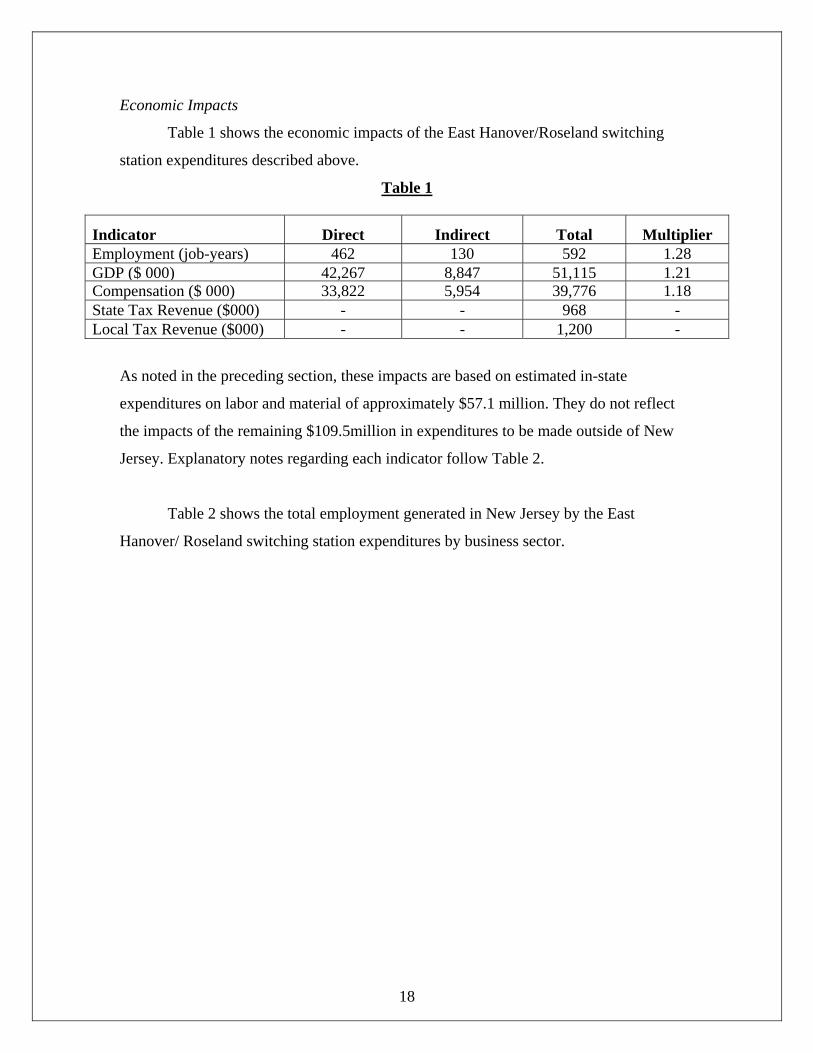
Economic Impacts
Table 1 shows the economic impacts of the East Hanover/Roseland switching
station expenditures described above.
Table 1
Indicator Direct Indirect Total Multiplier Employment (job-years) 462 130 592 1.28 GDP ($ 000) 42,267 8,847 51,115 1.21Compensation ($ 000) 33,822 5,954 39,776 1.18 State Tax Revenue ($000) - - 968 - Local Tax Revenue ($000) - - 1,200 -
As noted in the preceding section, these impacts are based on estimated in-state
expenditures on labor and material of approximately $57.1 million. They do not reflect
the impacts of the remaining $109.5million in expenditures to be made outside of New
Jersey. Explanatory notes regarding each indicator follow Table 2.
Table 2 shows the total employment generated in New Jersey by the East
Hanover/ Roseland switching station expenditures by business sector.

19
Table 2
Sector Employment (job-years)
Natural Resources & Mining 1 Construction 411 Manufacturing 27 Transportation & Public Utilities 12 Wholesale Trade 9 Retail Trade 29 Financial Activities 23 Services 79 Government 0 Total 592
• Employment
Employment impacts are measured in job-years (i.e., one job lasting one year).
The East Hanover/Roseland switching station portion of the project is estimated
to generate a total of 592 jobs in New Jersey. Based on salary and benefit
estimates for the employment required to construct the stations, approximately
411 direct construction jobs are estimated to be created. Note also from Table 1
that the direct employment associated with the construction of the switching
station (462 jobs) exceeds the total construction employment (411 jobs) listed in
Table 2. The additional direct employment (51 jobs) associated with the project is
generated in the New Jersey-based wholesale and manufacturing sectors that
produce and distribute the non-specialized materials used in laying foundations,
building access roads, etc., as well as the various PSE&G internal functions
associated with project management and support, and outside services (e.g., legal)
provided by New Jersey firms. Significant additional indirect employment (130
jobs, Table 1) is generated across various sectors, including services, financial
activities, and retail trade.
• GDP
As with the expenditures on construction of the transmission line, the GDP
generated in the state ($51.1 million) is close to the total expenditures estimated
for New Jersey due to the exclusion from the model of those material

20
expenditures that are to be made outside of New Jersey. The per-million-dollar
impacts reported below reflect the impact on New Jersey per million dollars of
total expenditures, including those expenditures made outside of the state.
• Compensation
Compensation represents the total wages, salaries and supplements to wages and
salaries (i.e., employer contributions to government and private pension funds)
paid for all direct and indirect jobs generated as a result of the project
expenditures made in New Jersey. The construction of the East
Hanover/Roseland switching station is estimated to generate $39.8 million in
compensation in New Jersey.
• State Tax Revenues
State tax revenues are comprised of the income taxes associated with the salaries
paid to the workers in the direct and indirect jobs associated with the project, and
with the sales associated with the economic output generated by the project. The
construction of the East Hanover/ Roseland switching station is estimated to
generate $.968 million in state tax revenues.
• Local Tax Revenues
Local tax revenues are comprised of increased property tax revenues resulting
from improvements associated with the increased business activity generated by
the project. The construction of the East Hanover/Roseland switching station is
estimated to generate $1.120 million in local tax revenues.
Table 3 provides the per-million-dollar spending impacts for the East
Hanover/Roseland switching station. Note that these impacts are calculated per million
dollars of total expenditures – that is, on the basis of the $166.6 million to be spent both
inside and outside of New Jersey.

21
Table 3
Indicator Impacts per $1 million of total expenditures
Employment (job-years) 3.6 GDP 306,785 Compensation 238,730 State Tax Revenues 5,811 Local Tax Revenues 7,202
22
Jefferson Switching Station
Expenditure Assumptions
In order to reflect the full range of expenditures incorporated into PSE&G’s cost
estimates for construction of the Jefferson switching station portion of the upgraded
Susquehanna-Roseland network, it was necessary to make several assumptions and
adjustments to the various expenditure items listed for construction of the station.
Following is an explanation of this process.
The total cost of construction for the East Hanover/Roseland switching
station was estimated at $77 million, including $57.8 million in base costs,
$6.1 million in escalation costs and $13.1 million in contingency.
The escalation (10.5%) and contingency (22.7%) estimates were
distributed proportionately between the contractor’s labor and material
costs. The Professional Services costs and the PSE&G Support costs were
distributed according to their respective shares of the $57.8 million base
cost.
The Scope Assessment and Fees on the labor portion of the contractor’s
costs (34% of base costs) were combined with the labor costs.
Expenditures on circuit breakers, disconnect switches, and third party
professional services were assumed to be made outside of New Jersey.
Of the approximately $6.5 million in bulk material expenditures, 60% was
assumed to be electrical material, and 40% civil material, with 90% of the
electrical bulk being purchased outside New Jersey. The majority of civil
bulk material associated with site work, access roads, foundations, etc.,
was assumed to be purchased in New Jersey.
23
All direct construction labor was assumed to come from North Jersey.
As a result of these assumptions and adjustments, $62.1 million of the
total $77 million estimate for construction (or 80.5%) of the Jefferson
Switching Station was allocated to expenditures on labor, services and
material in New Jersey.
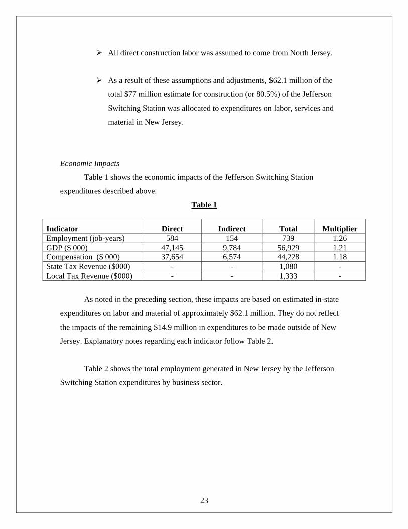
Economic Impacts
Table 1 shows the economic impacts of the Jefferson Switching Station
expenditures described above.
Table 1
Indicator Direct Indirect Total Multiplier Employment (job-years) 584 154 739 1.26 GDP ($ 000) 47,145 9,784 56,929 1.21Compensation ($ 000) 37,654 6,574 44,228 1.18 State Tax Revenue ($000) - - 1,080 - Local Tax Revenue ($000) - - 1,333 -
As noted in the preceding section, these impacts are based on estimated in-state
expenditures on labor and material of approximately $62.1 million. They do not reflect
the impacts of the remaining $14.9 million in expenditures to be made outside of New
Jersey. Explanatory notes regarding each indicator follow Table 2.
Table 2 shows the total employment generated in New Jersey by the Jefferson
Switching Station expenditures by business sector.

24
Table 2
Sector Employment (job-years)
Natural Resources & Mining 1 Construction 538 Manufacturing 26 Transportation & Public Utilities 12 Wholesale Trade 10 Retail Trade 47 Financial Activities 24 Services 80 Government 0 Total 739
• Employment
Employment impacts are measured in job-years (i.e., one job lasting one year).
The Jefferson Switching Station of the project is estimated to generate a total of
739 jobs in New Jersey. Based on salary and benefit estimates for the
employment required to construct the stations, approximately 538 direct
construction jobs are estimated to be created. Note also from Table 1 that the
direct employment associated with the construction of the Switching Stations
(584 jobs) exceeds the total construction employment (538 jobs) listed in Table 2.
The additional direct employment (46 jobs) associated with the project is
generated in the New Jersey-based wholesale and manufacturing sectors that
produce and distribute the non-specialized materials used in laying foundations,
building access roads, etc., as well as the various PSE&G internal functions
associated with project management and support, and outside services (e.g., legal)
provided by New Jersey firms. Significant additional indirect employment (154
jobs, Table 1) is generated across various sectors, including services, financial
activities, and retail trade.
• GDP
As with the expenditures on construction of the transmission line, the GDP
generated in the state ($56.9 million) is close to the total expenditures estimated
for New Jersey due to the exclusion from the model of those material

25
expenditures that are to be made outside of New Jersey. The per-million-dollar
impacts reported below reflect the impact on New Jersey per million dollars of
total expenditures, including those expenditures made outside of the state.
• Compensation
Compensation represents the total wages, salaries and supplements to wages and
salaries (i.e., employer contributions to government and private pension funds)
paid for all direct and indirect jobs generated as a result of the project
expenditures made in New Jersey. The construction of the Jefferson Switching
Station is estimated to generate $44.2 million in compensation in New Jersey.
• State Tax Revenues
State tax revenues are comprised of the income taxes associated with the salaries
paid to the workers in the direct and indirect jobs associated with the project, and
with the sales associated with the economic output generated by the project. The
construction of the Jefferson Switching Station is estimated to generate $1.1
million in state tax revenues.
• Local Tax Revenues
Local tax revenues are comprised of increased property tax revenues resulting
from improvements associated with the increased business activity generated by
the project. The construction of the Jefferson Switching Station is estimated to
generate $1.3 million in local tax revenues.
Table 3 provides the per-million-dollar spending impacts for the Jefferson
Switching Station. Note that these impacts are calculated per million dollars of total
transmission line expenditures – that is, on the basis of the $77 million to be spent both
inside and outside of New Jersey.

26
Table 3
Indicator Impacts per $1 million of total expenditures
Employment (job-years) 9.6 GDP $739,340 Compensation $574,392 State Tax Revenues $14,022 Local Tax Revenues $17,315
Note that these per-million-dollar impacts are significantly higher than those of
the East Hanover and Roseland stations. This is largely due to the fact that $70 million
dollars of expenditures on transformers and circuit breakers for the East Hanover and
Roseland stations is assumed to be spent out of state, while there are no comparable
expenditures for the Jefferson switching station. Thus, there is less economic “leakage”
assumed as a proportion of the total costs of construction.
27
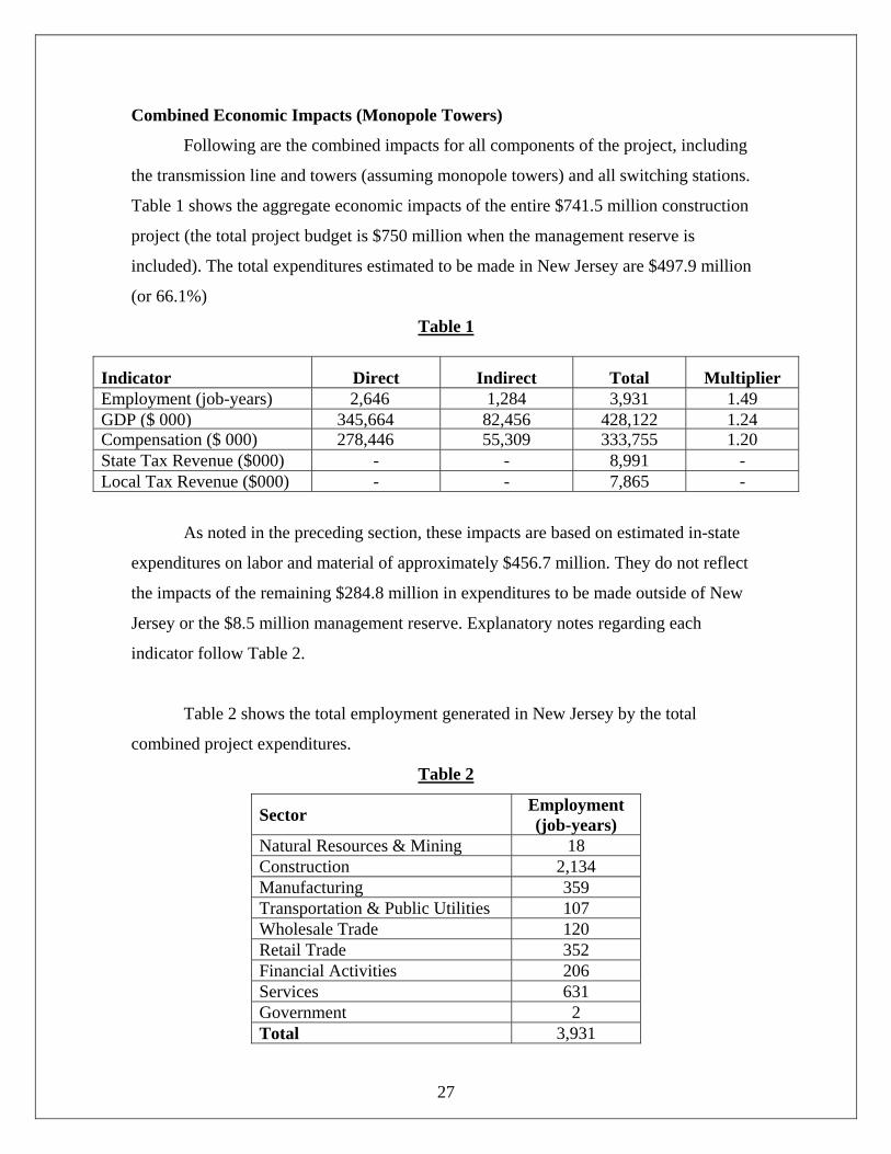
Combined Economic Impacts (Monopole Towers)
Following are the combined impacts for all components of the project, including
the transmission line and towers (assuming monopole towers) and all switching stations.
Table 1 shows the aggregate economic impacts of the entire $741.5 million construction
project (the total project budget is $750 million when the management reserve is
included). The total expenditures estimated to be made in New Jersey are $497.9 million
(or 66.1%)
Table 1
Indicator Direct Indirect Total Multiplier Employment (job-years) 2,646 1,284 3,931 1.49 GDP ($ 000) 345,664 82,456 428,122 1.24Compensation ($ 000) 278,446 55,309 333,755 1.20 State Tax Revenue ($000) - - 8,991 - Local Tax Revenue ($000) - - 7,865 -
As noted in the preceding section, these impacts are based on estimated in-state
expenditures on labor and material of approximately $456.7 million. They do not reflect
the impacts of the remaining $284.8 million in expenditures to be made outside of New
Jersey or the $8.5 million management reserve. Explanatory notes regarding each
indicator follow Table 2.
Table 2 shows the total employment generated in New Jersey by the total
combined project expenditures.
Table 2
Sector Employment (job-years)
Natural Resources & Mining 18 Construction 2,134 Manufacturing 359 Transportation & Public Utilities 107 Wholesale Trade 120 Retail Trade 352 Financial Activities 206 Services 631 Government 2 Total 3,931

28
• Employment
Total employment generated by the project is estimated at 3,931 jobs, with the
majority of those jobs occurring in the construction industry (2,143 jobs). Other
sectors with large direct and indirect job gains include the aggregate services
sector (631 jobs), the retail trade sector (352 jobs), and the manufacturing sector
(359 jobs).
• GDP
The GDP generated in the state ($428.1 million) is close to the total expenditures
estimated for New Jersey due to the exclusion from the model of those material
expenditures that are to be made outside of New Jersey. The per-million-dollar
impacts reported below reflect the impact on New Jersey per million dollars of
total expenditures, including those expenditures made outside of the state.
• Compensation
Compensation represents the total wages, salaries and supplements to wages and
salaries (i.e., employer contributions to government and private pension funds)
paid for all direct and indirect jobs generated as a result of the project
expenditures made in New Jersey. The project is estimated to generate $333.8
million in compensation in New Jersey.
• State Tax Revenues
State tax revenues are comprised of the income taxes associated with the salaries
paid to the workers in the direct and indirect jobs associated with the project, and
with the sales taxes associated with the economic output generated by the project.
The project is estimated to generate $9 million in state tax revenues.
• Local Tax Revenues
Local tax revenues are comprised of increased property tax revenues that are
generated over time because of property improvements associated with the
increased business activity generated by the project. The value of these property

29
improvements is, in time, included in assessments and hence in property tax
revenues. The project is estimated to generate $7.9 million in local tax revenues.
Table 3 provides the per-million-dollar spending impacts for the full project.
Note that these impacts are calculated per million dollars of total expenditures – that is,
on the basis of the $741.5 million to be spent both inside and outside of New Jersey and
including the additional $8.5 million management reserve.
Table 3
Indicator Impacts per $1 million of total expenditures
Employment (job-years) 5.2 GDP $570,829 Compensation $445,007 State Tax Revenues $11,988 Local Tax Revenues $10,487
30
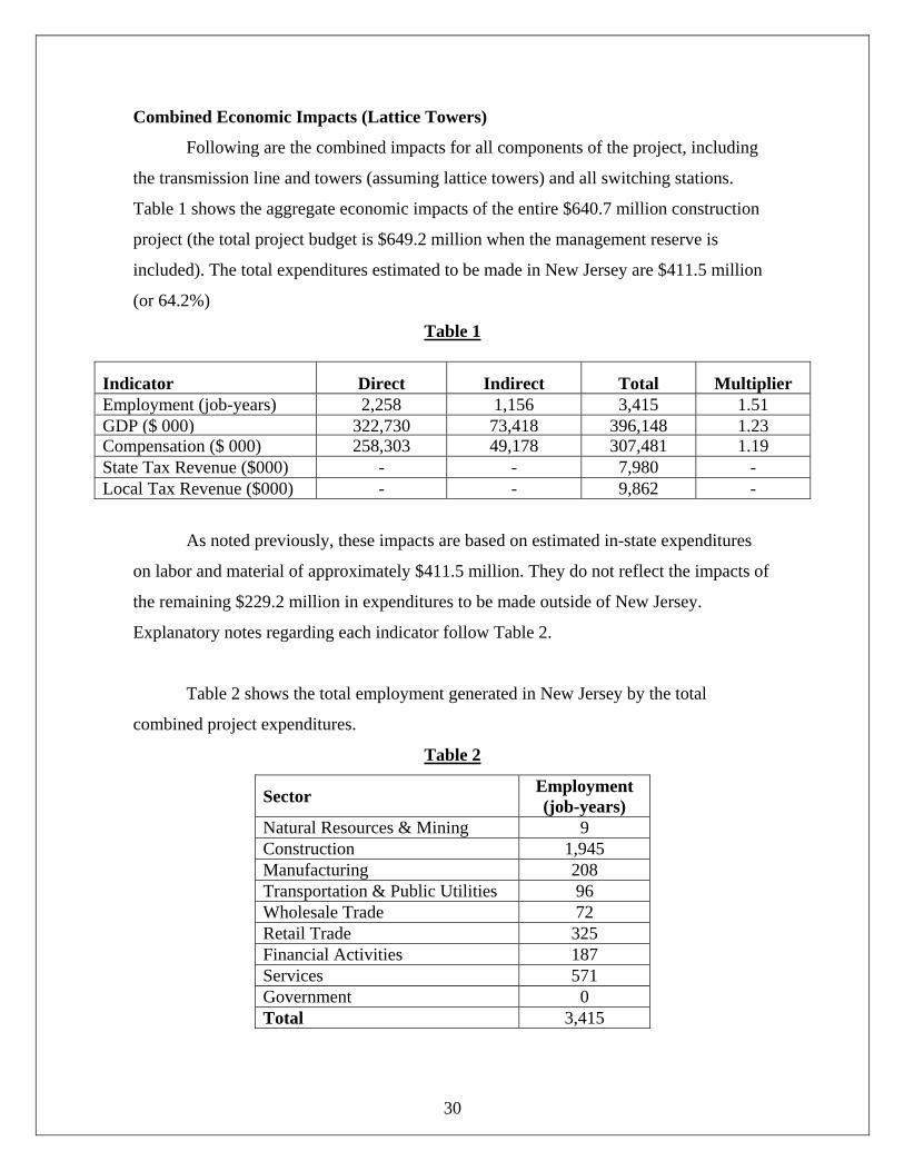
Combined Economic Impacts (Lattice Towers)
Following are the combined impacts for all components of the project, including
the transmission line and towers (assuming lattice towers) and all switching stations.
Table 1 shows the aggregate economic impacts of the entire $640.7 million construction
project (the total project budget is $649.2 million when the management reserve is
included). The total expenditures estimated to be made in New Jersey are $411.5 million
(or 64.2%)
Table 1
Indicator Direct Indirect Total Multiplier Employment (job-years) 2,258 1,156 3,415 1.51 GDP ($ 000) 322,730 73,418 396,148 1.23Compensation ($ 000) 258,303 49,178 307,481 1.19 State Tax Revenue ($000) - - 7,980 - Local Tax Revenue ($000) - - 9,862 -
As noted previously, these impacts are based on estimated in-state expenditures
on labor and material of approximately $411.5 million. They do not reflect the impacts of
the remaining $229.2 million in expenditures to be made outside of New Jersey.
Explanatory notes regarding each indicator follow Table 2.
Table 2 shows the total employment generated in New Jersey by the total
combined project expenditures.
Table 2
Sector Employment (job-years)
Natural Resources & Mining 9 Construction 1,945 Manufacturing 208 Transportation & Public Utilities 96 Wholesale Trade 72 Retail Trade 325 Financial Activities 187 Services 571 Government 0 Total 3,415
31
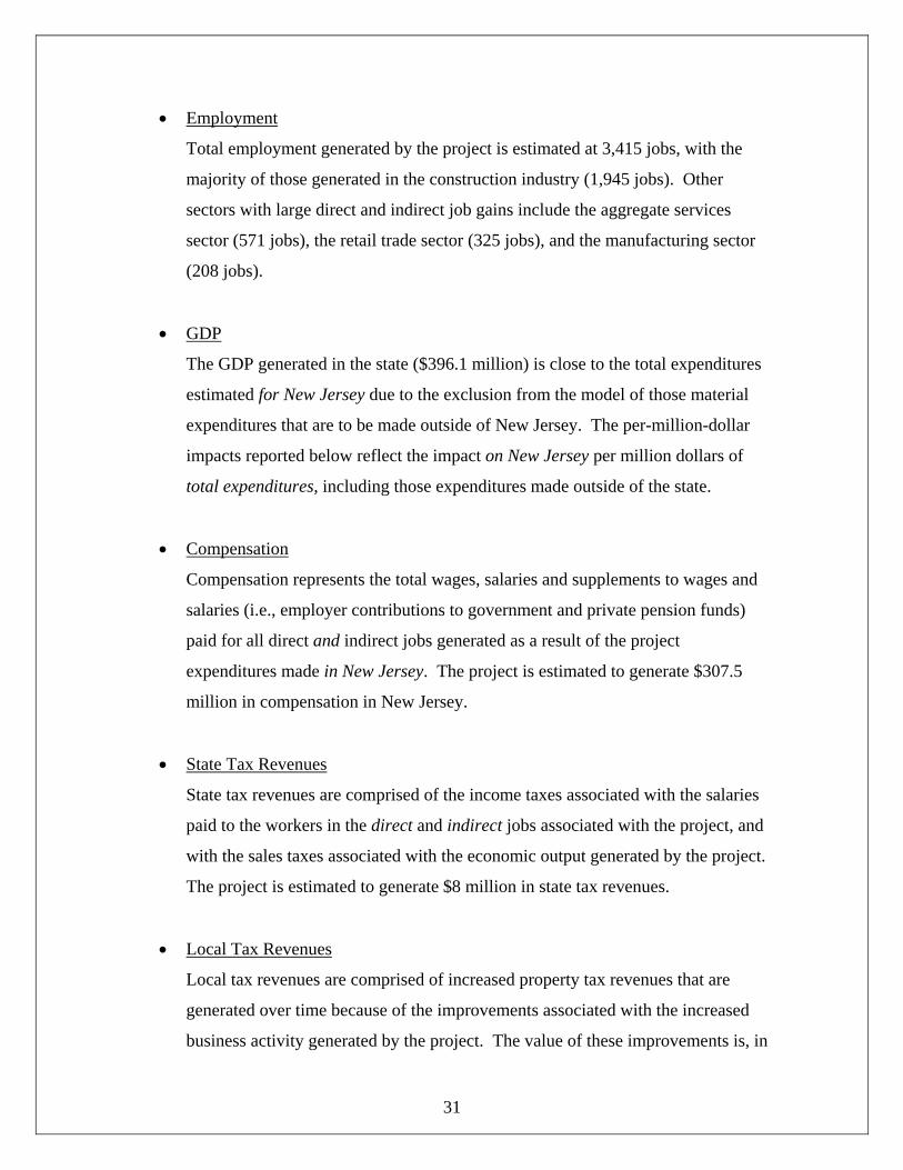
• Employment
Total employment generated by the project is estimated at 3,415 jobs, with the
majority of those generated in the construction industry (1,945 jobs). Other
sectors with large direct and indirect job gains include the aggregate services
sector (571 jobs), the retail trade sector (325 jobs), and the manufacturing sector
(208 jobs).
• GDP
The GDP generated in the state ($396.1 million) is close to the total expenditures
estimated for New Jersey due to the exclusion from the model of those material
expenditures that are to be made outside of New Jersey. The per-million-dollar
impacts reported below reflect the impact on New Jersey per million dollars of
total expenditures, including those expenditures made outside of the state.
• Compensation
Compensation represents the total wages, salaries and supplements to wages and
salaries (i.e., employer contributions to government and private pension funds)
paid for all direct and indirect jobs generated as a result of the project
expenditures made in New Jersey. The project is estimated to generate $307.5
million in compensation in New Jersey.
• State Tax Revenues
State tax revenues are comprised of the income taxes associated with the salaries
paid to the workers in the direct and indirect jobs associated with the project, and
with the sales taxes associated with the economic output generated by the project.
The project is estimated to generate $8 million in state tax revenues.
• Local Tax Revenues
Local tax revenues are comprised of increased property tax revenues that are
generated over time because of the improvements associated with the increased
business activity generated by the project. The value of these improvements is, in

32
time, included in assessments and hence in property taxes. The project is
estimated to generate $9.9 million in local tax revenues.
Table 3 provides the per-million-dollar spending impacts for the full project,
assuming all lattice tower structures are used for the transmission line. Note that these
impacts are calculated per million dollars of total expenditures – that is, on the basis of
the $640.7 million to be spent both inside and outside of New Jersey and including the
additional $8.5 million management reserve.
Table 3
Indicator Impacts per $1 million of total expenditures
Employment (job-years) 5.3 GDP $610,220 Compensation $473,639 State Tax Revenues $12,292 Local Tax Revenues $15,191
33
CONCLUSION
This report presents an economic impact analysis of the proposed upgrade of
PSE&G’s Susquehanna-Roseland transmission network. Using the Edward J. Bloustein
School’s R/ECON™ Input-Output model, impact estimates were generated for
construction of two switching stations and the transmission line and towers, including
separate analyses for two different types of tower. Based on the proposed employment
and other project expenditures to be made in New Jersey, we estimate that the $649.2
million (all lattice towers) to $750 million (all monopole towers) in project expenditures
($425.2 million to $467.7 million to be made in New Jersey), including management
reserves, will generate:
• between 3,415 (lattice) and 3,931 (monopole) job-years for workers in New
Jersey;
• between $396.1 million (lattice ) and $428.1 million (monopole) in gross
domestic product for the state;
• between $307.5 million (lattice) and $333.8 million in compensation for workers
in the jobs generated by the project in New Jersey;
• between $8 million (lattice) and $9 million (monopole) in state taxes; and
• between $7.9 million (monopole) and $9.9 million (lattice) in local taxes.

34
APPENDIX A: ECONOMIC AND DEMOGRAPHIC PROFILES AND DYNAMICS
The four counties where the transmission line work will occur – Essex, Morris,
Sussex, and Warren – together represent a microcosm of New Jersey, mirroring the
economic and demographic profile of the state, as well as the basic economic and
demographic dynamics of change. The four-county region has dense urban job and
residential concentrations, strong suburban job growth corridors and residential
communities, and dispersed rural-suburban territories characterized by very low density
development patterns.
The four-county economies are dominated by private service-providing
employment. The most significant service-providing sectors, in order of importance, are
trade, transportation, and utilities, professional and business services, and education and
health services. Employment growth rates in the four-county region have been relatively
modest, somewhat below those of the state, with education and health services the
leading growth sector.
Slow-growth demographics also characterize the four counties, with population
increases steadily declining through the decade. The principal reason for this slowdown
has been growing net migration losses – more people moving out than moving in – that
have now spread to even the low density counties of Sussex and Warren. The modest
population gains for the decade to date are due solely to net natural increase (births minus
deaths).
This Appendix examines the employment composition of the each of the counties
and the aggregated four-county region in the context of that of New Jersey as a whole, as
well as the patterns of change during the 2002-2008 period. This will be followed by a
demographic analysis of 2000-2008 period in terms of the basic components of
population change.
State, County, and Region Employment Analysis
The economies of Essex, Morris, Sussex, and Warren counties in total accounted
for nearly one-fifth (18.2 percent) of New Jersey’s total payroll employment in 2008
(730,495 jobs out of a state total of 4,007,911 jobs). Essex was the largest (363,038 jobs)

35
of the four counties, followed by Morris (289,095 jobs). Much smaller in size are Sussex
(40,407 jobs) and Warren (37,955 jobs). In general, Essex tends to have a concentrated
urban employment base (as well as a secondary suburban one), while that of Morris is
largely suburban highway-corridor oriented. Thus, Essex is the densest economy,
followed by Morris. In contrast, employment in Sussex has a much less dense and more
dispersed suburban-rural pattern. Warren is a mixture of urban, suburban, and rural, with
much of the county similar to Sussex. However, there is an older manufacturing base
centered in the area around Phillipsburg. Thus, the employment geography of the four-
county region is quite heterogeneous in terms of geographic distribution and density,
mirroring quite closely that of New Jersey in its entirety.
This is much less the case in the composition and growth patterns of each county.
The broad general job dynamic in the 2002-2008 period has been employment growth in
private-service providing activities and government, and employment declines in goods-
producing industries. The sector that dominated private-sector growth was education and
health services. This stands as a microcosm of what has occurred in the New Jersey
economy.
Employment Data
To analyze the four counties, New Jersey as a whole will serve as the baseline.
The source of both county and statewide data is the Quarterly Census of Employment and
Wages (QCEW) produced by the U.S. Bureau of Labor Statistics. At the state level, the
QCEW differs slightly from the Current Employment Survey (CES) payroll employment
series, which is sample-based and is released monthly by the New Jersey Department of
Labor and Workforce Development. The advantage of the QCEW is that it is a full count
and not a sample, and is available at the county level; its disadvantage is that the data are
not as current as the CES. The state data in the QCEW are the sum of the 21 counties.
The analysis begins in the second quarter of 2002 and ends in the second quarter
of 2008, the last quarter of data availability. The period of measurement was designed to
have the beginning and end points at similar stages in the business cycle. New Jersey’s
employment had peaked in December 2000, the end of the great economic expansion of

36
the 1990s. It then contracted through early 2003, when growth resumed. Employment
then kept expanding until it once again peaked, in December 2007, when the current
recession began. So both the beginning and end points (second quarter of 2002 and
second quarter of 2008) were in recessionary periods, with a modest economic expansion
in between.
Employment is classified into categories defined by the North American Industry
Classification System (NAICS). The initial partition is between the private sector and the
public sector (government). The private sector is further disaggregated into good-
producing industries and service-providing industries. There are three major goods-
producing industries – natural resources and mining, construction, and manufacturing.
Of the three, manufacturing is the largest.
There are seven major industries in the service-providing group: trade,
transportation, and utilities; information; financial activities; professional and business
services; education and health services; leisure and hospitality; and other services. The
three largest are trade, transportation, and utilities, professional and business services,
and educational and health services. The smallest is information. We will refer to them
as sectors or classifications. The following is a more detailed, but not complete,
definition of these sectors.
Trade, Transportation, and Utilities include wholesale trade, retail trade, transportation,
warehousing, and utilities.
Information includes publishing, telecommunications, Internet service providers, and
data processing activities.
Financial Activities include finance, insurance, and real estate.
Professional and Business Services includes professional, scientific, and technical
services; legal and accounting services; architectural and engineering services,
advertising, management of companies and enterprises, and administrative support.
37
Education and Health Services includes private education, health care, and social
assistance.
Leisure and Hospitality includes arts, entertainment, recreation, gambling, amusements,
accommodations, and food services and drinking places.
Other Services include repair and maintenance, personal and laundry services, and
religious, grant making, civic, professional and similar organizations.
The Baseline New Jersey Employment Growth Pattern
Between 2002 Q2 and 2008 Q2, total employment in New Jersey increased by
111,377 jobs or 2.9 percent, from 3.9 million to 4.0 million (Table 1). This 2.9 percent
growth was considerably below the national 7.2 percent increase for the same time
period.
Employment growth in the state was concentrated in both the private service-
providing sector (+134,173 jobs or +4.9 percent) and government (+34,445 jobs or +5.7
percent). Public-sector employment growth, while smaller in absolute magnitude than
private service-providing employment growth, had a higher rate of increase (5.7 percent
versus 4.8 percent).
In contrast, employment in the private goods-producing sector declined by 57,241
jobs or -10.6 percent. This decline was largely due to the state’s long-term
manufacturing hemorrhage. New Jersey lost 64,377 manufacturing jobs between 2002
and 2008, or -17.6 percent. Thus, nearly one out five of the state’s manufacturing jobs
disappeared in a brief six-year period. In the goods-producing sector, this loss was only
partially counter-balanced by growth in construction employment (+6,315 jobs or +3.9
percent).
Education and health services had the largest employment increase of all of the
service-providing industries. Between 2002 Q2 and 2008 Q2, this sector gained 72,285
jobs, a rate of increase of 15.1 percent, and it accounted for 64.9 percent of the state’s
total employment growth (72,285 jobs out of 111,377 jobs). It was followed by leisure
and hospitality (+41,553 jobs), professional and business services (+40,139 jobs), other
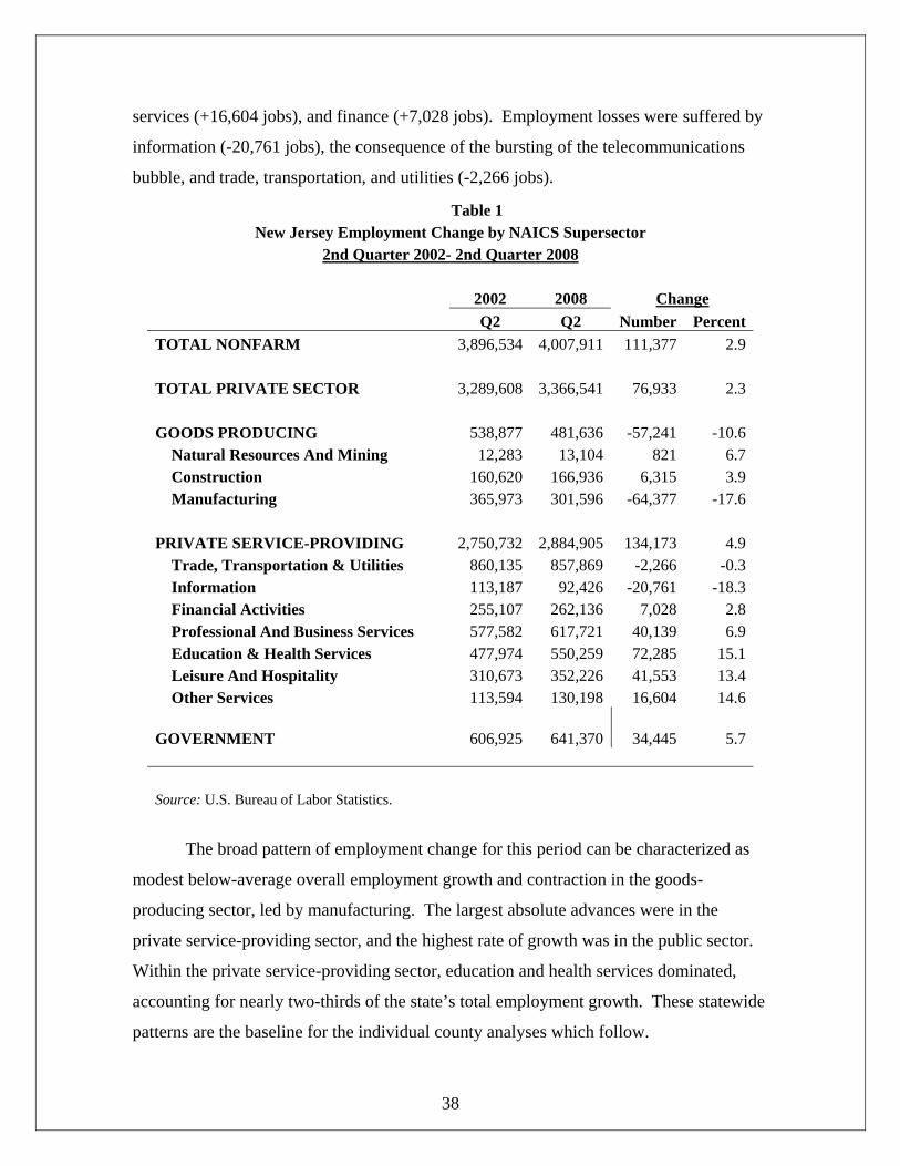
38
services (+16,604 jobs), and finance (+7,028 jobs). Employment losses were suffered by
information (-20,761 jobs), the consequence of the bursting of the telecommunications
bubble, and trade, transportation, and utilities (-2,266 jobs).
Table 1 New Jersey Employment Change by NAICS Supersector
2nd Quarter 2002- 2nd Quarter 2008 2002 2008 Change Q2 Q2 Number PercentTOTAL NONFARM 3,896,534 4,007,911 111,377 2.9 TOTAL PRIVATE SECTOR 3,289,608 3,366,541 76,933 2.3 GOODS PRODUCING 538,877 481,636 -57,241 -10.6
Natural Resources And Mining 12,283 13,104 821 6.7Construction 160,620 166,936 6,315 3.9Manufacturing 365,973 301,596 -64,377 -17.6
PRIVATE SERVICE-PROVIDING 2,750,732 2,884,905 134,173 4.9
Trade, Transportation & Utilities 860,135 857,869 -2,266 -0.3Information 113,187 92,426 -20,761 -18.3Financial Activities 255,107 262,136 7,028 2.8Professional And Business Services 577,582 617,721 40,139 6.9Education & Health Services 477,974 550,259 72,285 15.1Leisure And Hospitality 310,673 352,226 41,553 13.4Other Services 113,594 130,198 16,604 14.6
GOVERNMENT 606,925 641,370 34,445 5.7 Source: U.S. Bureau of Labor Statistics.
The broad pattern of employment change for this period can be characterized as
modest below-average overall employment growth and contraction in the goods-
producing sector, led by manufacturing. The largest absolute advances were in the
private service-providing sector, and the highest rate of growth was in the public sector.
Within the private service-providing sector, education and health services dominated,
accounting for nearly two-thirds of the state’s total employment growth. These statewide
patterns are the baseline for the individual county analyses which follow.
39
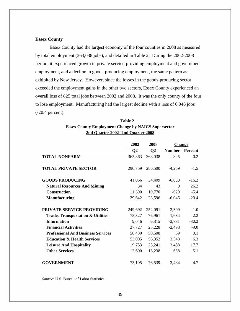
Essex County
Essex County had the largest economy of the four counties in 2008 as measured
by total employment (363,038 jobs), and detailed in Table 2. During the 2002-2008
period, it experienced growth in private service-providing employment and government
employment, and a decline in goods-producing employment, the same pattern as
exhibited by New Jersey. However, since the losses in the goods-producing sector
exceeded the employment gains in the other two sectors, Essex County experienced an
overall loss of 825 total jobs between 2002 and 2008. It was the only county of the four
to lose employment. Manufacturing had the largest decline with a loss of 6,046 jobs
(-20.4 percent).
Table 2 Essex County Employment Change by NAICS Supersector
2nd Quarter 2002- 2nd Quarter 2008 2002 2008 Change Q2 Q2 Number PercentTOTAL NONFARM 363,863 363,038 -825 -0.2 TOTAL PRIVATE SECTOR 290,759 286,500 -4,259 -1.5 GOODS PRODUCING 41,066 34,409 -6,658 -16.2
Natural Resources And Mining 34 43 9 26.2Construction 11,390 10,770 -620 -5.4Manufacturing 29,642 23,596 -6,046 -20.4
PRIVATE SERVICE-PROVIDING 249,692 252,091 2,399 1.0
Trade, Transportation & Utilities 75,327 76,961 1,634 2.2Information 9,046 6,315 -2,731 -30.2Financial Activities 27,727 25,228 -2,498 -9.0Professional And Business Services 50,439 50,508 69 0.1Education & Health Services 53,005 56,352 3,348 6.3Leisure And Hospitality 19,753 23,241 3,488 17.7Other Services 12,600 13,238 638 5.1
GOVERNMENT 73,105 76,539 3,434 4.7 Source: U.S. Bureau of Labor Statistics.

40
Leisure and hospitality had the highest employment gain (+3,488 jobs), followed
closely by education and health services (+3,348 jobs) and government (+3,434 jobs).
The loss of information employment in Essex County (-2,731 jobs) occurred at a rate
greater than that of New Jersey (-30.2 percent versus -18.3 percent). In direct contrast to
the state, Essex County lost employment in financial activities (-2,498 jobs). Also in
contrast to New Jersey, Essex County gained employment in trade, transportation, and
utilities (+1,634 jobs), led by booming port, logistical, and distribution activities. And its
modest gain in professional and business services – just 69 jobs (+0.1 percent) – stood in
marked contrast to strong growth statewide (6.9 percent).
Essex stands as the county employment-growth laggard, with pronounced job
losses in manufacturing, information, and finance. Leisure and hospitality, education and
health services, and government were the dominant growth sectors.
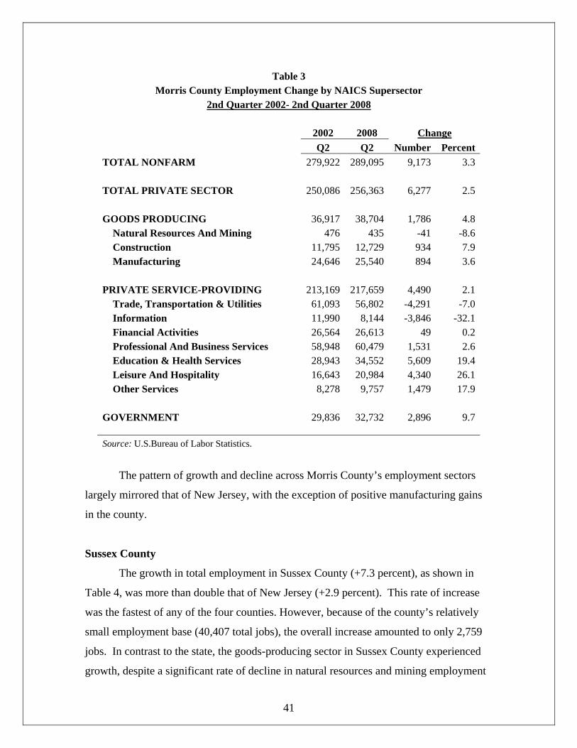
Morris County
Morris County ranked second among the four counties in total employment in
2008 (289,095 jobs), as shown in Table 3. Between 2002 and 2008, employment in
Morris County grew slightly faster than in New Jersey (3.3 percent versus 2.9 percent).
Its growth profile is very similar to that of the state as a whole with one exception –
manufacturing (Table 4). Morris County actually added 894 manufacturing jobs between
2002 and 2008 (+3.6 percent), largely due to the modest expansion of the pharmaceutical
industry, which is mostly categorized under manufacturing. As a result, the goods-
producing sector experienced positive growth (+4.8 percent) in sharp contrast to New
Jersey’s decline (-10.6 percent).
Similar to the state, Morris County had employment declines in two of the seven
service-providing sectors – trade, transportation, and utilities (-4,291 jobs) and
information (-3,846 jobs). Of the five growth sectors, education and health services had
the strongest gains (+5,609 jobs), followed by leisure and hospitality (+4,430 jobs), other
services (+1,479 jobs), professional and business services (+1,531 jobs), and finance (+49
jobs). Government employment (+2,896 jobs) grew at a rate higher than the state (+9.7
percent versus 5.7 percent).
41
Table 3 Morris County Employment Change by NAICS Supersector
2nd Quarter 2002- 2nd Quarter 2008 2002 2008 Change Q2 Q2 Number PercentTOTAL NONFARM 279,922 289,095 9,173 3.3 TOTAL PRIVATE SECTOR 250,086 256,363 6,277 2.5 GOODS PRODUCING 36,917 38,704 1,786 4.8
Natural Resources And Mining 476 435 -41 -8.6Construction 11,795 12,729 934 7.9Manufacturing 24,646 25,540 894 3.6
PRIVATE SERVICE-PROVIDING 213,169 217,659 4,490 2.1
Trade, Transportation & Utilities 61,093 56,802 -4,291 -7.0Information 11,990 8,144 -3,846 -32.1Financial Activities 26,564 26,613 49 0.2Professional And Business Services 58,948 60,479 1,531 2.6Education & Health Services 28,943 34,552 5,609 19.4Leisure And Hospitality 16,643 20,984 4,340 26.1Other Services 8,278 9,757 1,479 17.9
GOVERNMENT 29,836 32,732 2,896 9.7 Source: U.S.Bureau of Labor Statistics.
The pattern of growth and decline across Morris County’s employment sectors
largely mirrored that of New Jersey, with the exception of positive manufacturing gains
in the county.
Sussex County
The growth in total employment in Sussex County (+7.3 percent), as shown in
Table 4, was more than double that of New Jersey (+2.9 percent). This rate of increase
was the fastest of any of the four counties. However, because of the county’s relatively
small employment base (40,407 total jobs), the overall increase amounted to only 2,759
jobs. In contrast to the state, the goods-producing sector in Sussex County experienced
growth, despite a significant rate of decline in natural resources and mining employment

42
(-24.7 percent). Manufacturing employment was basically flat, while construction had
strong growth (+198 jobs or +8.3 percent).
Table 4 Sussex County Employment Change by NAICS Supersector
2nd Quarter 2002- 2nd Quarter 2008 2002 2008 Change Q2 Q2 Number PercentTOTAL NONFARM 37,648 40,407 2,759 7.3 TOTAL PRIVATE SECTOR 30,394 32,147 1,753 5.8 GOODS PRODUCING 4,519 4,689 170 3.8
Natural Resources And Mining 151 114 -37 -24.7Construction 2,388 2,586 198 8.3Manufacturing 1,980 1,989 9 0.5
PRIVATE SERVICE-PROVIDING 25,875 27,458 1,583 6.1
Trade, Transportation & Utilities 7,512 7,195 -317 -4.2Information 482 476 -6 -1.2Financial Activities 1,186 1,451 265 22.3Professional And Business Services 4,876 4,726 -151 -3.1Education & Health Services 5,796 6,729 933 16.1Leisure And Hospitality 4,346 4,673 326 7.5Other Services 1,333 1,764 431 32.4
GOVERNMENT 7,254 8,260 1,006 13.9 Source: U.S. Bureau of Labor Statistics.
Government (+1,006 jobs) was the biggest individual growth sector. It was
followed by education and health services (+933 jobs), other services (+431 jobs), leisure
and hospitality (+326 jobs), and financial services (+265 jobs). Employment contracted
in trade, transportation, and utilities (-317 jobs), professional and business services (-151
jobs), and information (-6 jobs).
While employment growth was faster than the state, the pattern of Sussex County
employment changes was generally consistent with the state growth template, with two
major differences. First, the county experienced surprising losses in professional and

43
business services employment, and second, its manufacturing sector demonstrated job
stability in contrast to the significant losses experienced statewide.
Warren County
Warren County has the smallest economy, comprising just 37,955 jobs in 2008, as
detailed in Table 5. This total was slightly below that of Sussex County (40,407 jobs).
Its overall employment growth rate (+3.2 percent or +1,186 jobs) between 2002 and 2008
was slightly above that of the state (+2.9 percent). The general statewide pattern of
growth in service-providing and government employment, and decline in goods-
producing employment was also evident in Warren County.
Table 5 Warren County Employment Change by NAICS Supersector
2nd Quarter 2002- 2nd Quarter 2008 2002 2008 Change Q2 Q2 Number Percent TOTAL NONFARM 36,770 37,955 1,186 3.2 TOTAL PRIVATE SECTOR 30,881 31,350 469 1.5 GOODS PRODUCING 8,525 8,175 -350 -4.1
Natural Resources And Mining 286 387 101 35.2Construction 1,476 1,953 477 32.3Manufacturing 6,762 5,834 -928 -13.7
PRIVATE SERVICE-PROVIDING 22,356 23,175 819 3.7
Trade, Transportation & Utilities 8,968 8,418 -550 -6.1Information 305 336 31 10.1Financial Activities 954 897 -57 -5.9Professional And Business Services 2,590 2,750 160 6.2Education & Health Services 5,181 6,220 1,039 20.1Leisure And Hospitality 2,976 3,115 138 4.6Other Services 1,125 1,361 236 20.9
GOVERNMENT 5,889 6,606 717 12.2 Source: U.S. Bureau of Labor Statistics.
44
Within the goods-producing sector, which lost 350 jobs, the decline in
manufacturing employment (-928 jobs) overweighed the combined growth in
construction (+477 jobs) and in natural resources and mining (+101 jobs). In the service-
providing sector (+819 jobs), education and health services added 1,039 jobs (+20.1
percent), the highest of any private-sector employment category. Also growing at above-
state average rates were other services (+20.9 percent or +236 jobs), information (+10.1
percent or +31 jobs), professional and business services (+6.2 percent or 160 jobs), and
leisure and hospitality (+4.6 percent or 138 jobs). Employment losses were suffered in
trade, transportation, and utilities (-550 jobs) and financial activities (-57 jobs).
Government employment, grew by 717 jobs (+12.2 percent).
Warren County’s growth pattern during the 2002 and 2008 period was much more
dominated by government compared to New Jersey. Government accounted for 60.4
percent of Warren’s total employment growth (717 jobs out of a total 1,186 jobs). For
New Jersey as a whole, government accounted for 30.9 percent (34,445 jobs out of
111,377 jobs). While there were some minor differences in several sectors, the same
dynamic of goods-producing employment contraction and service-providing employment
expansion was evident in both Warren County and New Jersey.
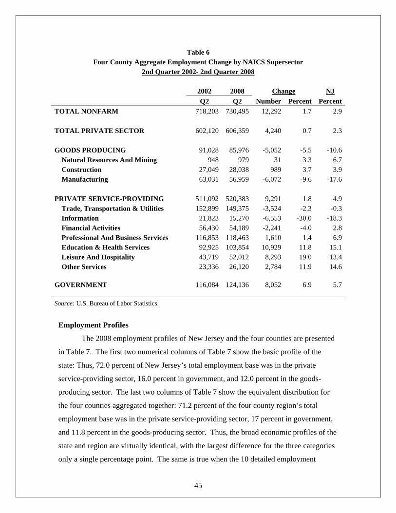
The Four County Region
Table 6 provides the four county aggregate employment levels and change for the
2002-2008 period, along with the percentage change for the state as a whole.
Employment in he four counties combined is growing somewhat slower than the New
Jersey, mainly due to mature Essex County, which is virtually built out. But outside of
this distinction, aggregating the four counties together tends to mute the individual
county differences. This aggregation results in a region where the broad patterns of
change – or the order of magnitude of the changes – are relatively close to those of the
state as a whole. Thus, the region strongly mirrors New Jersey.
45
Table 6 Four County Aggregate Employment Change by NAICS Supersector
2nd Quarter 2002- 2nd Quarter 2008 2002 2008 Change NJ Q2 Q2 Number Percent PercentTOTAL NONFARM 718,203 730,495 12,292 1.7 2.9 TOTAL PRIVATE SECTOR 602,120 606,359 4,240 0.7 2.3 GOODS PRODUCING 91,028 85,976 -5,052 -5.5 -10.6
Natural Resources And Mining 948 979 31 3.3 6.7Construction 27,049 28,038 989 3.7 3.9Manufacturing 63,031 56,959 -6,072 -9.6 -17.6
PRIVATE SERVICE-PROVIDING 511,092 520,383 9,291 1.8 4.9
Trade, Transportation & Utilities 152,899 149,375 -3,524 -2.3 -0.3Information 21,823 15,270 -6,553 -30.0 -18.3Financial Activities 56,430 54,189 -2,241 -4.0 2.8Professional And Business Services 116,853 118,463 1,610 1.4 6.9Education & Health Services 92,925 103,854 10,929 11.8 15.1Leisure And Hospitality 43,719 52,012 8,293 19.0 13.4Other Services 23,336 26,120 2,784 11.9 14.6
GOVERNMENT 116,084 124,136 8,052 6.9 5.7 Source: U.S. Bureau of Labor Statistics.
Employment Profiles
The 2008 employment profiles of New Jersey and the four counties are presented
in Table 7. The first two numerical columns of Table 7 show the basic profile of the
state: Thus, 72.0 percent of New Jersey’s total employment base was in the private
service-providing sector, 16.0 percent in government, and 12.0 percent in the goods-
producing sector. The last two columns of Table 7 show the equivalent distribution for
the four counties aggregated together: 71.2 percent of the four county region’s total
employment base was in the private service-providing sector, 17 percent in government,
and 11.8 percent in the goods-producing sector. Thus, the broad economic profiles of the
state and region are virtually identical, with the largest difference for the three categories
only a single percentage point. The same is true when the 10 detailed employment
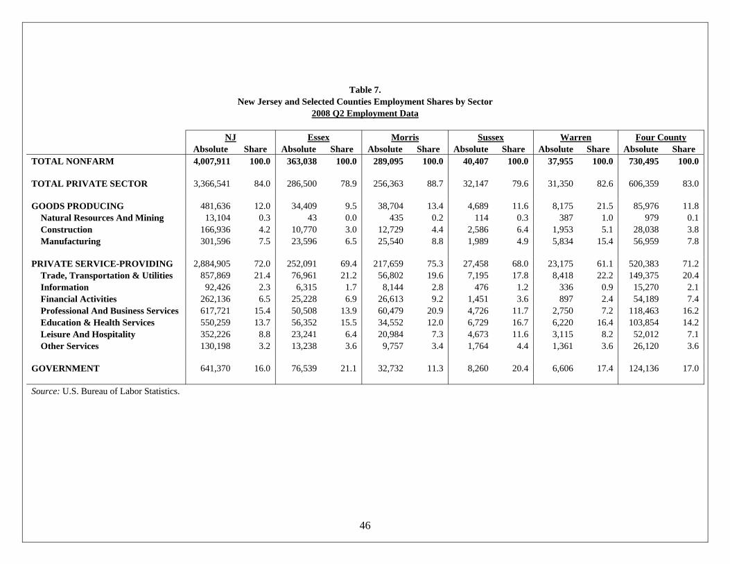
46
Table 7. New Jersey and Selected Counties Employment Shares by Sector
2008 Q2 Employment Data
NJ Essex Morris Sussex Warren Four County Absolute Share Absolute Share Absolute Share Absolute Share Absolute Share Absolute Share TOTAL NONFARM 4,007,911 100.0 363,038 100.0 289,095 100.0 40,407 100.0 37,955 100.0 730,495 100.0 TOTAL PRIVATE SECTOR 3,366,541 84.0 286,500 78.9 256,363 88.7 32,147 79.6 31,350 82.6 606,359 83.0 GOODS PRODUCING 481,636 12.0 34,409 9.5 38,704 13.4 4,689 11.6 8,175 21.5 85,976 11.8
Natural Resources And Mining 13,104 0.3 43 0.0 435 0.2 114 0.3 387 1.0 979 0.1 Construction 166,936 4.2 10,770 3.0 12,729 4.4 2,586 6.4 1,953 5.1 28,038 3.8 Manufacturing 301,596 7.5 23,596 6.5 25,540 8.8 1,989 4.9 5,834 15.4 56,959 7.8
PRIVATE SERVICE-PROVIDING 2,884,905 72.0 252,091 69.4 217,659 75.3 27,458 68.0 23,175 61.1 520,383 71.2
Trade, Transportation & Utilities 857,869 21.4 76,961 21.2 56,802 19.6 7,195 17.8 8,418 22.2 149,375 20.4 Information 92,426 2.3 6,315 1.7 8,144 2.8 476 1.2 336 0.9 15,270 2.1 Financial Activities 262,136 6.5 25,228 6.9 26,613 9.2 1,451 3.6 897 2.4 54,189 7.4 Professional And Business Services 617,721 15.4 50,508 13.9 60,479 20.9 4,726 11.7 2,750 7.2 118,463 16.2 Education & Health Services 550,259 13.7 56,352 15.5 34,552 12.0 6,729 16.7 6,220 16.4 103,854 14.2 Leisure And Hospitality 352,226 8.8 23,241 6.4 20,984 7.3 4,673 11.6 3,115 8.2 52,012 7.1 Other Services 130,198 3.2 13,238 3.6 9,757 3.4 1,764 4.4 1,361 3.6 26,120 3.6
GOVERNMENT 641,370 16.0 76,539 21.1 32,732 11.3 8,260 20.4 6,606 17.4 124,136 17.0 Source: U.S. Bureau of Labor Statistics.

47
sectors are compared. In only two sectors – trade, transportation, and utilities (1.0
percentage points) and leisure and hospitality (1.7 percentage points) – is the difference
in share equal to or greater than a single percentage point. The difference in share for the
other eight detailed sectors is less than a single percentage point.
There is much more variation when the individual county profiles are compared to
the state and with one another. Morris County has the highest share of its total
employment in the service-providing sector (75.3 percent) while Warren County had the
lowest share (61.1 percent). In contrast, Warren County had the highest share of its total
employment in the goods-producing sector (21.5 percent), while Essex had the lowest
(9.5 percent). The government sector was most pronounced in Essex County, where it
accounted for 21.1 percent of total employment. In contrast, government accounted for
only 11.3 percent of total employment in Morris County.
Of the major individual sectors, construction employment had the greatest
proportional representation in Sussex County (6.4 percent of total employment) while
Essex County had the least (3.0 percent). Manufacturing employment had its greatest
proportional share in Warren County (15.4 percent) and its lowest in Sussex County (4.9
percent). Trade, transportation, and utilities employment had a much smaller variation
among the counties, with its share ranging from a low of 17.8 percent (Sussex County)
and a high of 22.2 percent (Warren County).
Information employment had its highest share in Morris County (2.8 percent) and
its lowest share in Warren County (0.9 percent). The same pattern prevailed in financial
activities and professional and business services employment. Morris County had the
greatest share of its total employment in financial activities (9.2 percent) and Warren
County had the lowest (2.4 percent). Similarly, Morris County had the highest share of
its total employment in professional and business services (20.9 percent) while Warren
County had the lowest (7.2 percent).
Education and health services employment had only minor variations in the four
counties relative to its 13.7 percent share of the state’s total employment, with the highest
share in Sussex County (16.7 percent) and the lowest share in Morris County (12.0
percent). The outliers in leisure and hospitality employment were Sussex County, where
this sector had the highest share (11.6 percent), and Essex County, where it had the

48
lowest share (6.4 percent). Other services’ share had small variations between 3.4
percent and 4.4 percent.
These distributional patterns reveal that the economies of the four individual
counties do reflect the economic structure of the state as a whole, but at the same time
they each have some unique features and specializations. Most importantly, Morris and
Essex counties each have large powerful office markets that compete with nation’s
largest metropolitan areas. Morris County ranked first among the 21 counties in the state
with more than 30.3 million square feet of office space, while Essex County ranks fourth
with 28.8 million square feet of office space. Thus, these two large counties have the
greatest concentrations of high-end jobs in information, finance, and professional and
business services. Sussex and Warren counties have very much smaller office
inventories, particularly Class A office buildings (the most attractive, technologically-
equipped, investment-grade properties). Information, finance and professional and
business services jobs in these two counties tend to be more population oriented, i.e.,
providing services to households and individuals, rather than serving much broader state
and national markets, as is the case in Morris and Essex counties.
Demographics
The four-county region in total accounted for 17.5 percent (1,519,008 persons out
of 8,682,661 persons) of New Jersey’s population in 2008, a slightly lower percentage
than its share of the state’s total payroll employment (18.2 percent). Essex County
dominated in terms of absolute size (770,675 persons), followed by Morris County
(487,548 persons), as shown in Table 8. Sussex County’s population totaled only
150,909 persons in 2008, while Warren County’s population was even smaller (109,875
persons). As was the case with employment, Essex County has the highest population
density, as it contains New Jersey’s largest city as well as some of its densest older
suburbs. Morris County is far more suburban in character, while Sussex County is
mostly low-density rural and secondarily suburban. Warren County is a mixture of
suburban and rural, with a small urbanized area surrounding Phillipsburg. So the
residential development and population density variations within the four-county region
tend mirror the wide variations evident in the state as a whole.
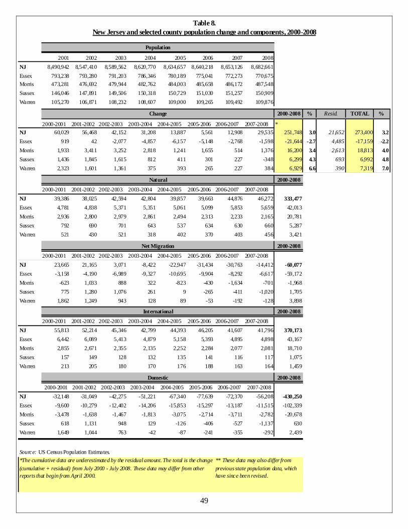
49
2001 2002 2003 2004 2005 2006 2007 2008NJ 8,490,942 8,547,410 8,589,562 8,620,770 8,634,657 8,640,218 8,653,126 8,682,661Essex 793,238 793,280 791,203 786,346 780,189 775,041 772,273 770,675Morris 473,281 476,692 479,944 482,762 484,003 485,658 486,172 487,548Sussex 146,046 147,891 149,506 150,318 150,729 151,030 151,257 150,909Warren 105,270 106,871 108,232 108,607 109,000 109,265 109,492 109,876
2000-2008 % Resid. TOTAL %
2000-2001 2001-2002 2002-2003 2003-2004 2004-2005 2005-2006 2006-2007 2007-2008 *NJ 60,029 56,468 42,152 31,208 13,887 5,561 12,908 29,535 251,748 3.0 21,652 273,400 3.2Essex 919 42 -2,077 -4,857 -6,157 -5,148 -2,768 -1,598 -21,644 -2.7 4,485 -17,159 -2.2Morris 1,933 3,411 3,252 2,818 1,241 1,655 514 1,376 16,200 3.4 2,613 18,813 4.0Sussex 1,436 1,845 1,615 812 411 301 227 -348 6,299 4.3 693 6,992 4.8Warren 2,323 1,601 1,361 375 393 265 227 384 6,929 6.6 390 7,319 7.0
2000-2008
2000-2001 2001-2002 2002-2003 2003-2004 2004-2005 2005-2006 2006-2007 2007-2008NJ 39,386 38,025 42,594 42,804 39,857 39,663 44,876 46,272 333,477Essex 4,781 4,838 5,371 5,351 5,061 5,099 5,853 5,659 42,013Morris 2,936 2,800 2,979 2,861 2,494 2,313 2,233 2,165 20,781Sussex 792 690 701 643 537 634 630 660 5,287Warren 521 430 521 318 402 370 403 456 3,421
2000-2008
2000-2001 2001-2002 2002-2003 2003-2004 2004-2005 2005-2006 2006-2007 2007-2008NJ 23,665 21,165 3,071 -8,422 -22,947 -31,434 -30,763 -14,412 -60,077Essex -3,158 -4,190 -6,989 -9,327 -10,695 -9,904 -8,292 -6,617 -59,172Morris -623 1,033 888 322 -823 -430 -1,634 -701 -1,968Sussex 775 1,280 1,076 261 9 -265 -411 -1,020 1,705Warren 1,862 1,249 943 128 89 -53 -192 -128 3,898
2000-2008
2000-2001 2001-2002 2002-2003 2003-2004 2004-2005 2005-2006 2006-2007 2007-2008NJ 55,813 52,214 45,346 42,799 44,393 46,205 41,607 41,796 370,173Essex 6,442 6,089 5,413 4,879 5,158 5,393 4,895 4,898 43,167Morris 2,855 2,671 2,355 2,135 2,252 2,284 2,077 2,081 18,710Sussex 157 149 128 132 135 141 116 117 1,075Warren 213 205 180 170 176 188 163 164 1,459
2000-2008
2000-2001 2001-2002 2002-2003 2003-2004 2004-2005 2005-2006 2006-2007 2007-2008NJ -32,148 -31,049 -42,275 -51,221 -67,340 -77,639 -72,370 -56,208 -430,250Essex -9,600 -10,279 -12,402 -14,206 -15,853 -15,297 -13,187 -11,515 -102,339Morris -3,478 -1,638 -1,467 -1,813 -3,075 -2,714 -3,711 -2,782 -20,678Sussex 618 1,131 948 129 -126 -406 -527 -1,137 630Warren 1,649 1,044 763 -42 -87 -241 -355 -292 2,439
Source: US Census Population Estimates.
Table 8.New Jersey and selected county population change and components, 2000-2008
Population
International
Net Migration
** These data may also differ from previous state population data, which have since been revised.
Change
Natural
Domestic
*The cumulative data are underestimated by the residual amount. The total is the change (cumulative + residual) from July 2000 - July 2008. These data may differ from other reports that begin from April 2000.

50
Table 8 also provides year-by year population levels for New Jersey and the four
counties, as well as the annual changes in population. Population change has three major
components: net natural increase (births minus deaths), net international immigration (the
difference between the number of people from outside the United States moving into
New Jersey and the number of people from New Jersey moving outside the country), and
net domestic migration (the difference between the number of people from New Jersey
moving to the rest of the United States and the number of people from the rest of the
country moving into New Jersey). Net migration is the sum of international and domestic
migration. All of these components are detailed in Table 8 for each county and the state.
A technical note is warranted here. When the Census Bureau tabulates this data,
the sum of the components (which yields the net annual population change) this
sometimes differs slightly from the net annual change as computed directly from annual
population totals. This difference is what the Census Bureau calls the residual. So the
final change data for the 2000-2008 period, presented in the far right column of Table 8,
includes the residual. Between 2000 and 2008, New Jersey’s population grew by
273,400 people (+3.2 percent), a pace far slower than that of the nation (+7.8 percent).
The four-county region had a 2000-2008 population growth of 15,965 persons (+1.1
percent). So, the four-county region was growing slower than New Jersey and far slower
than the United States (7.8 percent).
This is largely due to the absolute population decline that took place in Essex
County during this period (-17,159 persons or -2.2 percent). Positive growth was
registered by the other three counties, led by Warren County (+7,319 persons or +7.0
percent). It is important to note that even Warren County’s growth rate lagged that of the
nation. Sussex County had the second highest growth rate (+4.8 percent or +6,992
persons) followed closely by Morris County (+4.0 percent or 18,813 persons).
Much of this growth took place in the early years of the 2000-2008 period. For
example, New Jersey’s overall population increase totaled 60,029 persons in 2000-2001.
The annual net growth increment then steadily declined to just 5,561 persons in 2005-
2006, before rebounding in the next two years. The slowdown in growth was largely due
to a surge of domestic migration losses, from -32,148 persons in 2000-2001 to -77,639
51
persons in 2005-2006. So the wave of New Jerseyans moving to other states reduced the
state’s overall annual population growth almost down to zero by 2005-2006.
However, there was a growth rebound in the last two years of this period. This
rebound was due an increase in the natural component of population (births minus
deaths) which rose from 39,663 in 2005-2006 to 46,272 in 2007-2008. It was also caused
by a reduction in domestic mobility caused by the housing bust – if you can’t sell your
house, you can’t move. While New Jersey still had significant domestic outmigration
losses – -72,370 persons in 2006-2007 and -56,208 persons in 2007-2008 – this decline in
net domestic outmigration and the gain in the natural component of population growth
resulted in an increase in the state’s annual population growth to 29,535 persons in 2007-
2008.
As seen in Table 8, net domestic outmigration was initially restricted to Essex and
Morris counties through 2002-2003. Then in 2003-2004, they were joined by Warren
County. By 2004-2005, all four counties were experiencing net domestic migration
losses. And this remained the case for the years that followed: net domestic migration
losses were pervasive in 2005-2006, 2006-2007, and 2007-2008.
For the entire 2000-2008 period, net domestic out migration in New Jersey
(-430,250 persons) was greater than net international immigration (+370,000 persons),
which yielded an overall net migration loss (-60,077 persons). Thus all of the 2000-2008
total population growth in the state (+273,400 persons) was due to net natural increase
(+333,477 persons). This general pattern is reflected in the four-county region, where the
net domestic outmigration (-119,948 persons) was proportionally far greater than net
international immigration (+64,411). As was the case for the state as a whole, population
growth was solely due to net natural increase (+71,502 persons) since international
immigration did not fully counterbalance net domestic migration losses. Since, overall
net migration losses totaled 55,537 persons, the four-county population change totaled
15,965 persons.
To summarize, the four-counties combined had positive population growth
between 2000 and 2003. Starting in 2003-2004, the net annual population change turned
negative. This was largely due to population losses in Essex County. It was also caused
by sharply lower annual gains experienced by the other three counties. The four counties

52
combined now basically comprise a very slow-growth demographic region, with all four
individual counties currently experiencing net domestic migration losses. With the full
impact of the Highlands Act yet to be fully realized in terms of developmental growth
restrictions, the four counties are likely to be destined to remain on a slow-growth
population trajectory.
53
APPENDIX B: INPUT-OUTPUT ANALYSIS
This appendix discusses the history and application of input-output analysis and
details the input-output model, called the R/Econ™ I-O model, developed by Rutgers
University. This model offers significant advantages in detailing the total economic
effects of an activity (such as historic rehabilitation and heritage tourism), including
multiplier effects.
ESTIMATING MULTIPLIERS
The fundamental issue determining the size of the multiplier effect is the
“openness” of regional economies. Regions that are more “open” are those that import
their required inputs from other regions. Imports can be thought of as substitutes for local
production. Thus, the more a region depends on imported goods and services instead of
its own production, the more economic activity leaks away from the local economy.
Businessmen noted this phenomenon and formed local chambers of commerce with the
explicit goal of stopping such leakage by instituting a “buy local” policy among their
membership. In addition, during the 1970s, as an import invasion was under way,
businessmen and union leaders announced a “buy American” policy in the hope of
regaining ground lost to international economic competition. Therefore, one of the main
goals of regional economic multiplier research has been to discover better ways to
estimate the leakage of purchases out of a region or, relatedly, to determine the region’s
level of self-sufficiency.
The earliest attempts to systematize the procedure for estimating multiplier effects
used the economic base model, still in use in many econometric models today. This
approach assumes that all economic activities in a region can be divided into two
categories: “basic” activities that produce exclusively for export, and region-serving or
“local” activities that produce strictly for internal regional consumption. Since this
approach is simpler but similar to the approach used by regional input-output analysis, let
us explain briefly how multiplier effects are estimated using the economic base approach.
If we let x be export employment, l be local employment, and t be total employment, then
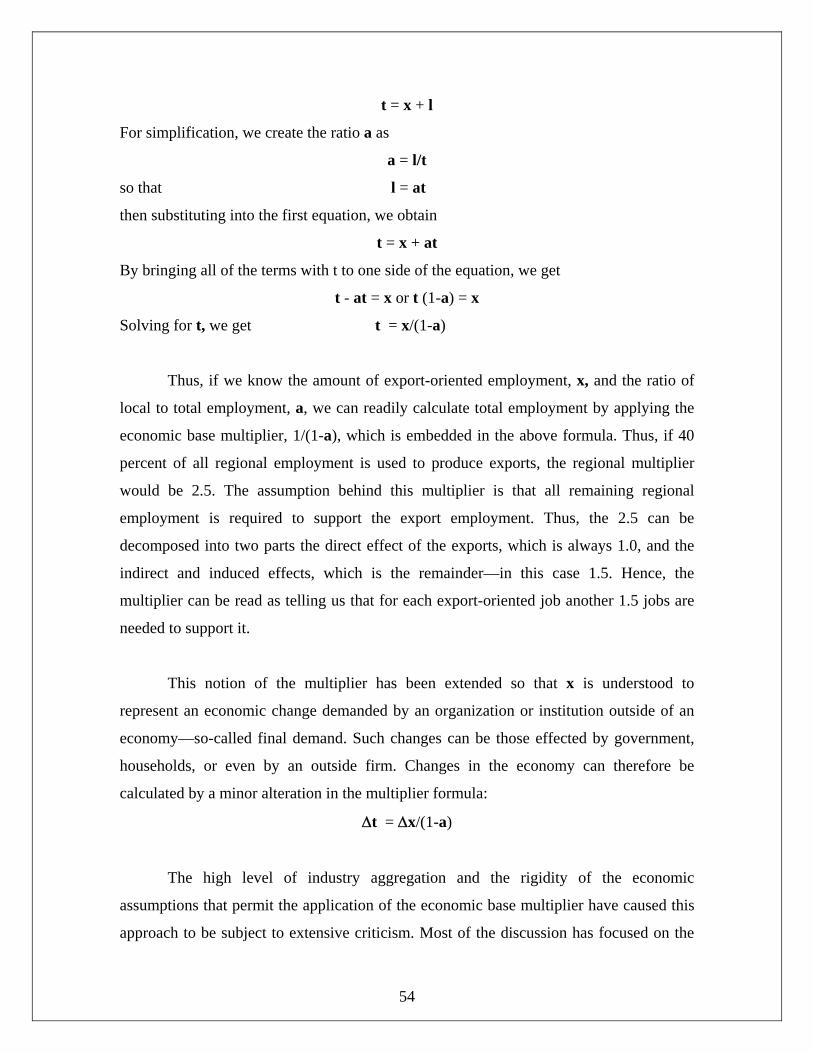
54
t = x + l
For simplification, we create the ratio a as
a = l/t
so that l = at
then substituting into the first equation, we obtain
t = x + at
By bringing all of the terms with t to one side of the equation, we get
t - at = x or t (1-a) = x
Solving for t, we get t = x/(1-a)
Thus, if we know the amount of export-oriented employment, x, and the ratio of
local to total employment, a, we can readily calculate total employment by applying the
economic base multiplier, 1/(1-a), which is embedded in the above formula. Thus, if 40
percent of all regional employment is used to produce exports, the regional multiplier
would be 2.5. The assumption behind this multiplier is that all remaining regional
employment is required to support the export employment. Thus, the 2.5 can be
decomposed into two parts the direct effect of the exports, which is always 1.0, and the
indirect and induced effects, which is the remainder—in this case 1.5. Hence, the
multiplier can be read as telling us that for each export-oriented job another 1.5 jobs are
needed to support it.
This notion of the multiplier has been extended so that x is understood to
represent an economic change demanded by an organization or institution outside of an
economy—so-called final demand. Such changes can be those effected by government,
households, or even by an outside firm. Changes in the economy can therefore be
calculated by a minor alteration in the multiplier formula:
Δt = Δx/(1-a)
The high level of industry aggregation and the rigidity of the economic
assumptions that permit the application of the economic base multiplier have caused this
approach to be subject to extensive criticism. Most of the discussion has focused on the
55
estimation of the parameter a. Estimating this parameter requires that one be able to
distinguish those parts of the economy that produce for local consumption from those that
do not. Indeed, virtually all industries, even services, sell to customers both inside and
outside the region. As a result, regional economists devised an approach by which to
measure the degree to which each industry is involved in the nonbase activities of the
region, better known as the industry’s regional purchase coefficient. Thus, they expanded
the above formulations by calculating for each i industry
li = r idi
and xi = ti - r idi
given that di is the total regional demand for industry i’s product. Given the above
formulae and data on regional demands by industry, one can calculate an accurate
traditional aggregate economic base parameter by the following:
a = l/t = Σlii/Σti
Although accurate, this approach only facilitates the calculation of an aggregate
multiplier for the entire region. That is, we cannot determine from this approach what the
effects are on the various sectors of an economy. This is despite the fact that one must
painstakingly calculate the regional demand as well as the degree to which they each
industry is involved in nonbase activity in the region.
As a result, a different approach to multiplier estimation that takes advantage of
the detailed demand and trade data was developed. This approach is called input-output
analysis.
REGIONAL INPUT-OUTPUT ANALYSIS: A BRIEF HISTORY
The basic framework for input-output analysis originated nearly 250 years ago
when François Quesenay published Tableau Economique in 1758. Quesenay’s “tableau”
graphically and numerically portrayed the relationships between sales and purchases of
the various industries of an economy. More than a century later, his description was

56
adapted by Leon Walras, who advanced input-output modeling by providing a concise
theoretical formulation of an economic system (including consumer purchases and the
economic representation of “technology”).
It was not until the twentieth century, however, that economists advanced and
tested Walras’s work. Wassily Leontief greatly simplified Walras’s theoretical formu-
lation by applying the Nobel prize–winning assumptions that both technology and trading
patterns were fixed over time. These two assumptions meant that the pattern of flows
among industries in an area could be considered stable. These assumptions permitted
Walras’s formulation to use data from a single time period, which generated a great
reduction in data requirements.
Although Leontief won the Nobel Prize in 1973, he first used his approach in
1936 when he developed a model of the 1919 and 1929 U.S. economies to estimate the
effects of the end of World War I on national employment. Recognition of his work in
terms of its wider acceptance and use meant development of a standardized procedure for
compiling the requisite data (today’s national economic census of industries) and
enhanced capability for calculations (i.e., the computer).
The federal government immediately recognized the importance of Leontief’s
development and has been publishing input-output tables of the U.S. economy since
1939. The most recently published tables are those for 1987. Other nations followed suit.
Indeed, the United Nations maintains a bank of tables from most member nations with a
uniform accounting scheme.
Framework
Input-output modeling focuses on the interrelationships of sales and purchases
among sectors of the economy. Input-output is best understood through its most basic
form, the interindustry transactions table or matrix. In this table (see figure 1 for an
example), the column industries are consuming sectors (or markets) and the row
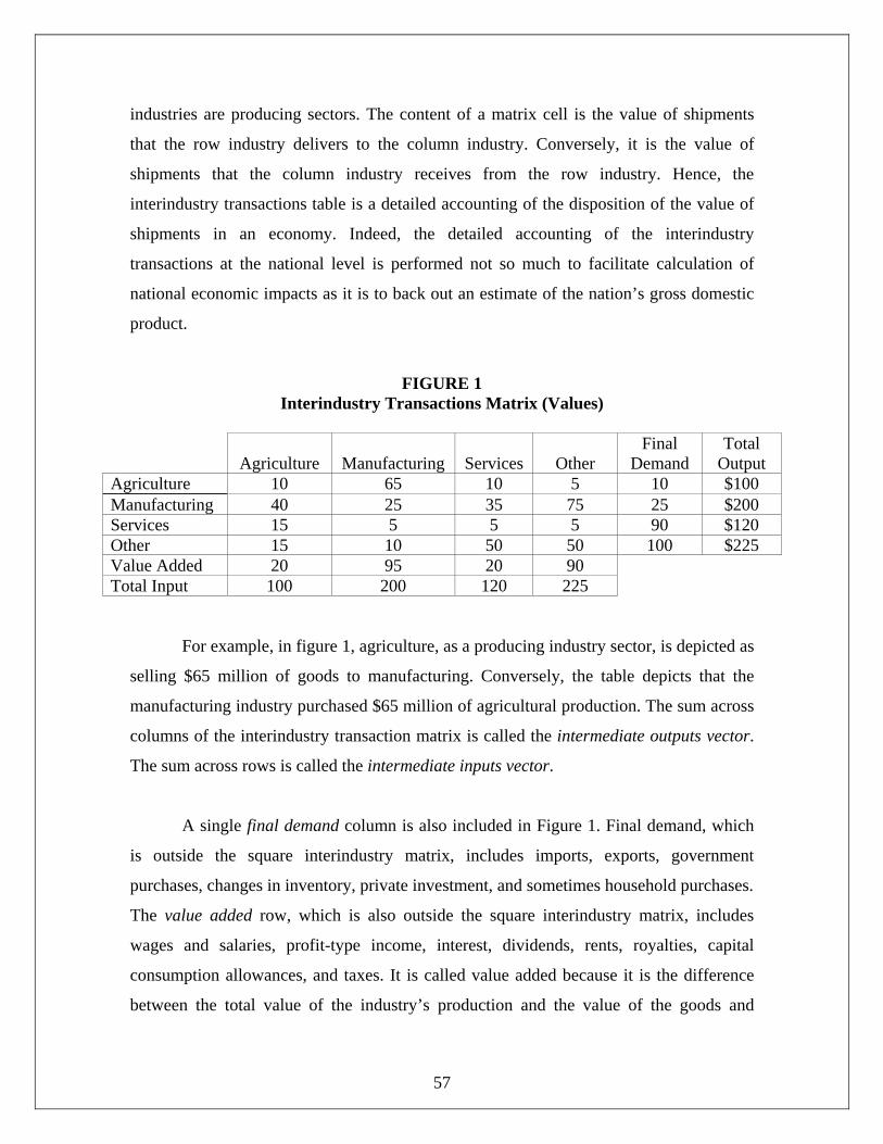
57
industries are producing sectors. The content of a matrix cell is the value of shipments
that the row industry delivers to the column industry. Conversely, it is the value of
shipments that the column industry receives from the row industry. Hence, the
interindustry transactions table is a detailed accounting of the disposition of the value of
shipments in an economy. Indeed, the detailed accounting of the interindustry
transactions at the national level is performed not so much to facilitate calculation of
national economic impacts as it is to back out an estimate of the nation’s gross domestic
product.
FIGURE 1 Interindustry Transactions Matrix (Values)
Agriculture
Manufacturing
Services
Other Final
Demand Total
Output Agriculture 10 65 10 5 10 $100 Manufacturing 40 25 35 75 25 $200 Services 15 5 5 5 90 $120 Other 15 10 50 50 100 $225 Value Added 20 95 20 90 Total Input 100 200 120 225
For example, in figure 1, agriculture, as a producing industry sector, is depicted as
selling $65 million of goods to manufacturing. Conversely, the table depicts that the
manufacturing industry purchased $65 million of agricultural production. The sum across
columns of the interindustry transaction matrix is called the intermediate outputs vector.
The sum across rows is called the intermediate inputs vector.
A single final demand column is also included in Figure 1. Final demand, which
is outside the square interindustry matrix, includes imports, exports, government
purchases, changes in inventory, private investment, and sometimes household purchases.
The value added row, which is also outside the square interindustry matrix, includes
wages and salaries, profit-type income, interest, dividends, rents, royalties, capital
consumption allowances, and taxes. It is called value added because it is the difference
between the total value of the industry’s production and the value of the goods and

58
nonlabor services that it requires to produce. Thus, it is the value that an industry adds to
the goods and services it uses as inputs in order to produce output.
The value added row measures each industry’s contribution to wealth
accumulation. In a national model, therefore, its sum is better known as the gross
domestic product (GDP). At the state level, this is known as the gross state product—a
series produced by the U.S. Bureau of Economic Analysis and published in the Regional
Economic Information System. Below the state level, it is known simply as the regional
equivalent of the GDP—the gross regional product.
Input-output economic impact modelers now tend to include the household
industry within the square interindustry matrix. In this case, the “consuming industry” is
the household itself. Its spending is extracted from the final demand column and is
appended as a separate column in the interindustry matrix. To maintain a balance, the
income of households must be appended as a row. The main income of households is
labor income, which is extracted from the value-added row. Modelers tend not to include
other sources of household income in the household industry’s row. This is not because
such income is not attributed to households but rather because much of this other income
derives from sources outside of the economy that is being modeled.
The next step in producing input-output multipliers is to calculate the direct
requirements matrix, which is also called the technology matrix. The calculations are
based entirely on data from figure 1. As shown in figure 2, the values of the cells in the
direct requirements matrix are derived by dividing each cell in a column of figure 1, the
interindustry transactions matrix, by its column total. For example, the cell for
manufacturing’s purchases from agriculture is 65/200 = .33. Each cell in a column of the
direct requirements matrix shows how many cents of each producing industry’s goods
and/or services are required to produce one dollar of the consuming industry’s production
and are called technical coefficients. The use of the terms “technology” and “technical”
derive from the fact that a column of this matrix represents a recipe for a unit of an
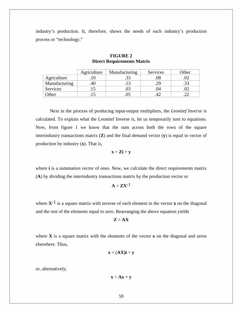
59
industry’s production. It, therefore, shows the needs of each industry’s production
process or “technology.”
FIGURE 2 Direct Requirements Matrix
Agriculture Manufacturing Services Other
Agriculture .10 .33 .08 .02 Manufacturing .40 .13 .29 .33 Services .15 .03 .04 .02 Other .15 .05 .42 .22
Next in the process of producing input-output multipliers, the Leontief Inverse is
calculated. To explain what the Leontief Inverse is, let us temporarily turn to equations.
Now, from figure 1 we know that the sum across both the rows of the square
interindustry transactions matrix (Z) and the final demand vector (y) is equal to vector of
production by industry (x). That is,
x = Zi + y
where i is a summation vector of ones. Now, we calculate the direct requirements matrix
(A) by dividing the interindustry transactions matrix by the production vector or
A = ZX-1
where X-1 is a square matrix with inverse of each element in the vector x on the diagonal
and the rest of the elements equal to zero. Rearranging the above equation yields
Z = AX
where X is a square matrix with the elements of the vector x on the diagonal and zeros
elsewhere. Thus,
x = (AX)i + y
or, alternatively,
x = Ax + y
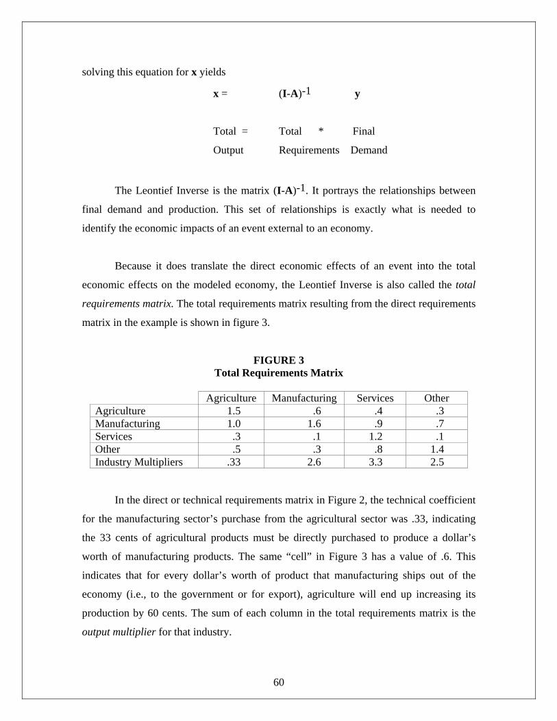
60
solving this equation for x yields
x = (I-A)-1 y
Total = Total * Final
Output Requirements Demand
The Leontief Inverse is the matrix (I-A)-1. It portrays the relationships between
final demand and production. This set of relationships is exactly what is needed to
identify the economic impacts of an event external to an economy.
Because it does translate the direct economic effects of an event into the total
economic effects on the modeled economy, the Leontief Inverse is also called the total
requirements matrix. The total requirements matrix resulting from the direct requirements
matrix in the example is shown in figure 3.
FIGURE 3 Total Requirements Matrix
Agriculture Manufacturing Services Other
Agriculture 1.5 .6 .4 .3 Manufacturing 1.0 1.6 .9 .7 Services .3 .1 1.2 .1 Other .5 .3 .8 1.4 Industry Multipliers .33 2.6 3.3 2.5
In the direct or technical requirements matrix in Figure 2, the technical coefficient
for the manufacturing sector’s purchase from the agricultural sector was .33, indicating
the 33 cents of agricultural products must be directly purchased to produce a dollar’s
worth of manufacturing products. The same “cell” in Figure 3 has a value of .6. This
indicates that for every dollar’s worth of product that manufacturing ships out of the
economy (i.e., to the government or for export), agriculture will end up increasing its
production by 60 cents. The sum of each column in the total requirements matrix is the
output multiplier for that industry.

61
Multipliers
A multiplier is defined as the system of economic transactions that follow a
disturbance in an economy. Any economic disturbance affects an economy in the same
way as does a drop of water in a still pond. It creates a large primary “ripple” by causing
a direct change in the purchasing patterns of affected firms and institutions. The suppliers
of the affected firms and institutions must change their purchasing patterns to meet the
demands placed upon them by the firms originally affected by the economic disturbance,
thereby creating a smaller secondary “ripple.” In turn, those who meet the needs of the
suppliers must change their purchasing patterns to meet the demands placed upon them
by the suppliers of the original firms, and so on; thus, a number of subsequent “ripples”
are created in the economy.
The multiplier effect has three components—direct, indirect, and induced effects.
Because of the pond analogy, it is also sometimes referred to as the ripple effect.
• A direct effect (the initial drop causing the ripple effects) is the change in purchases
due to a change in economic activity.
• An indirect effect is the change in the purchases of suppliers to those economic
activities directly experiencing change.
• An induced effect is the change in consumer spending that is generated by changes in
labor income within the region as a result of the direct and indirect effects of the
economic activity. Including households as a column and row in the interindustry
matrix allows this effect to be captured.
Extending the Leontief Inverse to pertain not only to relationships between total
production and final demand of the economy but also to changes in each permits its
multipliers to be applied to many types of economic impacts. Indeed, in impact analysis
the Leontief Inverse lends itself to the drop-in-a-pond analogy discussed earlier. This is
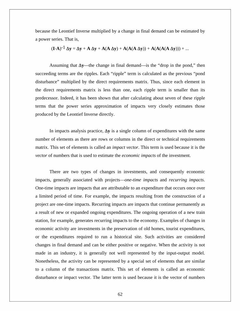
62
because the Leontief Inverse multiplied by a change in final demand can be estimated by
a power series. That is,
(I-A)-1 Δy = Δy + A Δy + A(A Δy) + A(A(A Δy)) + A(A(A(A Δy))) + ...
Assuming that Δy—the change in final demand—is the “drop in the pond,” then
succeeding terms are the ripples. Each “ripple” term is calculated as the previous “pond
disturbance” multiplied by the direct requirements matrix. Thus, since each element in
the direct requirements matrix is less than one, each ripple term is smaller than its
predecessor. Indeed, it has been shown that after calculating about seven of these ripple
terms that the power series approximation of impacts very closely estimates those
produced by the Leontief Inverse directly.
In impacts analysis practice, Δy is a single column of expenditures with the same
number of elements as there are rows or columns in the direct or technical requirements
matrix. This set of elements is called an impact vector. This term is used because it is the
vector of numbers that is used to estimate the economic impacts of the investment.
There are two types of changes in investments, and consequently economic
impacts, generally associated with projects—one-time impacts and recurring impacts.
One-time impacts are impacts that are attributable to an expenditure that occurs once over
a limited period of time. For example, the impacts resulting from the construction of a
project are one-time impacts. Recurring impacts are impacts that continue permanently as
a result of new or expanded ongoing expenditures. The ongoing operation of a new train
station, for example, generates recurring impacts to the economy. Examples of changes in
economic activity are investments in the preservation of old homes, tourist expenditures,
or the expenditures required to run a historical site. Such activities are considered
changes in final demand and can be either positive or negative. When the activity is not
made in an industry, it is generally not well represented by the input-output model.
Nonetheless, the activity can be represented by a special set of elements that are similar
to a column of the transactions matrix. This set of elements is called an economic
disturbance or impact vector. The latter term is used because it is the vector of numbers
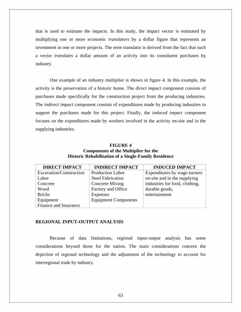
63
that is used to estimate the impacts. In this study, the impact vector is estimated by
multiplying one or more economic translators by a dollar figure that represents an
investment in one or more projects. The term translator is derived from the fact that such
a vector translates a dollar amount of an activity into its constituent purchases by
industry.
One example of an industry multiplier is shown in figure 4. In this example, the
activity is the preservation of a historic home. The direct impact component consists of
purchases made specifically for the construction project from the producing industries.
The indirect impact component consists of expenditures made by producing industries to
support the purchases made for this project. Finally, the induced impact component
focuses on the expenditures made by workers involved in the activity on-site and in the
supplying industries.
FIGURE 4 Components of the Multiplier for the
Historic Rehabilitation of a Single-Family Residence
DIRECT IMPACT INDIRECT IMPACT INDUCED IMPACT Excavation/Construction Labor Concrete Wood Bricks Equipment Finance and Insurance
Production Labor Steel Fabrication Concrete Mixing Factory and Office Expenses Equipment Components
Expenditures by wage earners on-site and in the supplying industries for food, clothing, durable goods, entertainment
REGIONAL INPUT-OUTPUT ANALYSIS
Because of data limitations, regional input-output analysis has some
considerations beyond those for the nation. The main considerations concern the
depiction of regional technology and the adjustment of the technology to account for
interregional trade by industry.
64
In the regional setting, local technology matrices are not readily available. An
accurate region-specific technology matrix requires a survey of a representative sample
of organizations for each industry to be depicted in the model. Such surveys are
extremely expensive.4 Because of the expense, regional analysts have tended to use
national technology as a surrogate for regional technology. This substitution does not
affect the accuracy of the model as long as local industry technology does not vary
widely from the nation’s average.5
Even when local technology varies widely from the nation’s average for one or
more industries, model accuracy may not be affected much. This is because interregional
trade may mitigate the error that would be induced by the technology. That is, in
estimating economic impacts via a regional input-output model, national technology must
be regionalized by a vector of regional purchase coefficients,6 r, in the following manner:
(I-rA)-1 r⋅Δy
or
r⋅Δy + rA (r⋅Δy) + rA(rA (r⋅Δy)) + rA(rA(rA (r⋅Δy))) + ...
where the vector-matrix product rA is an estimate of the region’s direct requirements
matrix. Thus, if national technology coefficients—which vary widely from their local
equivalents—are multiplied by small RPCs, the error transferred to the direct
requirements matrices will be relatively small. Indeed, since most manufacturing
industries have small RPCs and since technology differences tend to arise due to
substitution in the use of manufactured goods, technology differences have generally
been found to be minor source error in economic impact measurement. Instead, RPCs and
4The most recent statewide survey-based model was developed for the State of Kansas in 1986 and cost on the order of $60,000 (in 1990 dollars). The development of this model, however, leaned heavily on work done in 1965 for the same state. In addition the model was aggregated to the 35-sector level, making it inappropriate for many possible applications since the industries in the model do not represent the very detailed sectors that are generally analyzed. 5Only recently have researchers studied the validity of this assumption. They have found that large urban areas may have technology in some manufacturing industries that differs in a statistically significant way from the national average. As will be discussed in a subsequent paragraph, such differences may be unimportant after accounting for trade patterns. 6A regional purchase coefficient (RPC) for an industry is the proportion of the region’s demand for a good or service that is fulfilled by local production. Thus, each industry’s RPC varies between zero (0) and one (1), with one implying that all local demand is fulfilled by local suppliers. As a general rule, agriculture, mining, and manufacturing industries tend to have low RPCs, and both service and construction industries tend to have high RPCs.

65
their measurement error due to industry aggregation have been the focus of research on
regional input-output model accuracy.
A COMPARISON OF THREE MAJOR REGIONAL ECONOMIC IMPACT
MODELS
In the United States there are three major vendors of regional input-output
models. They are U.S. Bureau of Economic Analysis’s (BEA) RIMS II multipliers,
Minnesota IMPLAN Group Inc.’s (MIG) IMPLAN Pro model, and CUPR’s own
REcon™ I–O model. CUPR has had the privilege of using them all. (R/Econ™ I–O
builds from the PC I–O model produced by the Regional Science Research Corporation’s
(RSRC).)
Although the three systems have important similarities, there are also significant
differences that should be considered before deciding which system to use in a particular
study. This document compares the features of the three systems. Further discussion can
be found in Brucker, Hastings, and Latham’s article in the Summer 1987 issue of The
Review of Regional Studies entitled “Regional Input-Output Analysis: A Comparison of
Five Ready-Made Model Systems.” Since that date, CUPR and MIG have added a
significant number of new features to PC I–O (now, R/Econ™ I–O) and IMPLAN,
respectively.
Model Accuracy
RIMS II, IMPLAN, and RECON™ I–O all employ input-output (I–O) models for
estimating impacts. All three regionalized the U.S. national I–O technology coefficients
table at the highest levels of disaggregation (more than 500 industries). Since aggregation
of sectors has been shown to be an important source of error in the calculation of impact
multipliers, the retention of maximum industrial detail in these regional systems is a
positive feature that they share. The systems diverge in their regionalization approaches,
however. The difference is in the manner that they estimate regional purchase
66
coefficients (RPCs), which are used to regionalize the technology matrix. An RPC is the
proportion of the region’s demand for a good or service that is fulfilled by the region’s
own producers rather than by imports from producers in other areas. Thus, it expresses
the proportion of the purchases of the good or service that do not leak out of the region,
but rather feed back to its economy, with corresponding multiplier effects. Thus, the
accuracy of the RPC is crucial to the accuracy of a regional I–O model, since the regional
multiplier effects of a sector vary directly with its RPC.
The techniques for estimating the RPCs used by CUPR and MIG in their models
are theoretically more appealing than the location quotient (LQ) approach used in RIMS
II. This is because the former two allow for crosshauling of a good or service among
regions and the latter does not. Since crosshauling of the same general class of goods or
services among regions is quite common, the CUPR-MIG approach should provide better
estimates of regional imports and exports. Statistical results reported in Stevens, Treyz,
and Lahr (1989) confirm that LQ methods tend to overestimate RPCs. By extension,
inaccurate RPCs may lead to inaccurately estimated impact estimates.
Further, the estimating equation used by CUPR to produce RPCs should be more
accurate than that used by MIG. The difference between the two approaches is that MIG
estimates RPCs at a more aggregated level (two-digit SICs, or about 86 industries) and
applies them at a desegregate level (over 500 industries). CUPR both estimates and
applies the RPCs at the most detailed industry level. The application of aggregate RPCs
can induce as much as 50 percent error in impact estimates (Lahr and Stevens, 2002).
Although both RECON™ I–O and IMPLAN use an RPC-estimating technique
that is theoretically sound and update it using the most recent economic data, some
practitioners question their accuracy. The reasons for doing so are three-fold. First, the
observations currently used to estimate their implemented RPCs are based on 20-years
old trade relationships—the Commodity Transportation Survey (CTS) from the 1977
Census of Transportation. Second, the CTS observations are at the state level. Therefore,
RPC’s estimated for substate areas are extrapolated. Hence, there is the potential that
67
RPCs for counties and metropolitan areas are not as accurate as might be expected. Third,
the observed CTS RPCs are only for shipments of goods. The interstate provision of
services is unmeasured by the CTS. IMPLAN replies on relationships from the 1977 U.S.
Multiregional Input-Output Model that are not clearly documented. RECON™ I–O relies
on the same econometric relationships that it does for manufacturing industries but
employs expert judgment to construct weight/value ratios (a critical variable in the RPC-
estimating equation) for the nonmanufacturing industries.
The fact that BEA creates the RIMS II multipliers gives it the advantage of being
constructed from the full set of the most recent regional earnings data available. BEA is
the main federal government purveyor of employment and earnings data by detailed
industry. It therefore has access to the fully disclosed and disaggregated versions of these
data. The other two model systems rely on older data from County Business Patterns and
Bureau of Labor Statistic’s ES202 forms, which have been “improved” by filling-in for
any industries that have disclosure problems (this occurs when three or fewer firms exist
in an industry or a region).
Model Flexibility
For the typical user, the most apparent differences among the three modeling
systems are the level of flexibility they enable and the type of results that they yield.
R/Econ™ I–O allows the user to make changes in individual cells of the 515-by-515
technology matrix as well as in the 11 515-sector vectors of region-specific data that are
used to produce the regionalized model. The 11 sectors are: output, demand, employment
per unit output, labor income per unit output, total value added per unit of output, taxes
per unit of output (state and local), nontax value added per unit output, administrative and
auxiliary output per unit output, household consumption per unit of labor income, and the
RPCs. Te PC I–O model tends to be simple to use. Its User’s Guide is straightforward
and concise, providing instruction about the proper implementation of the model as well
as the interpretation of the model’s results.
68
The software for IMPLAN Pro is Windows-based, and its User’s Guide is more
formalized. Of the three modeling systems, it is the most user-friendly. The Windows
orientation has enabled MIG to provide many more options in IMPLAN without
increasing the complexity of use. Like R/Econ™ I–O, IMPLAN’s regional data on RPCs,
output, labor compensation, industry average margins, and employment can be revised. It
does not have complete information on tax revenues other than those from indirect
business taxes (excise and sales taxes), and those cannot be altered. Also like R/Econ™,
IMPLAN allows users to modify the cells of the 538-by-538 technology matrix. It also
permits the user to change and apply price deflators so that dollar figures can be updated
from the default year, which may be as many as four years prior to the current year. The
plethora of options, which are advantageous to the advanced user, can be extremely
confusing to the novice. Although default values are provided for most of the options, the
accompanying documentation does not clearly point out which items should get the most
attention. Further, the calculations needed to make any requisite changes can be more
complex than those needed for the R/Econ™ I–O model. Much of the documentation for
the model dwells on technical issues regarding the guts of the model. For example, while
one can aggregate the 538-sector impacts to the one- and two-digit SIC level, the current
documentation does not discuss that possibility. Instead, the user is advised by the Users
Guide to produce an aggregate model to achieve this end. Such a model, as was discussed
earlier, is likely to be error ridden.
For a region, RIMS II typically delivers a set of 38-by-471 tables of multipliers
for output, earnings, and employment; supplementary multipliers for taxes are available
at additional cost. Although the model’s documentation is generally excellent, use of
RIMS II alone will not provide proper estimates of a region’s economic impacts from a
change in regional demand. This is because no RPC estimates are supplied with the
model. For example, in order to estimate the impacts of rehabilitation, one not only needs
to be able to convert the engineering cost estimates into demands for labor as well as for
materials and services by industry, but must also be able to estimate the percentage of the
labor income, materials, and services which will be provided by the region’s households
and industries (the RPCs for the demanded goods and services). In most cases, such
69
percentages are difficult to ascertain; however, they are provided in the R/Econ™
I–O and IMPLAN models with simple triggering of an option. Further, it is impossible to
change any of the model’s parameters if superior data are known. This model ought not
to be used for evaluating any project or event where superior data are available or where
the evaluation is for a change in regional demand (a construction project or an event) as
opposed to a change in regional supply (the operation of a new establishment).
Model Results
Detailed total economic impacts for about 500 industries can be calculated for
jobs, labor income, and output from R/Econ™ I–O and IMPLAN only. These two
modeling systems can also provide total impacts as well as impacts at the one- and two-
digit industry levels. RIMS II provides total impacts and impacts on only 38 industries
for these same three measures. Only the manual for R/Econ™ I–O warns about the
problems of interpreting and comparing multipliers and any measures of output, also
known as the value of shipments.
As an alternative to the conventional measures and their multipliers, R/Econ™ I–
O and IMPLAN provide results on a measure known as “value added.” It is the region’s
contribution to the nation’s gross domestic product (GDP) and consists of labor income,
nonmonetary labor compensation, proprietors’ income, profit-type income, dividends,
interest, rents, capital consumption allowances, and taxes paid. It is, thus, the region’s
production of wealth and is the single best economic measure of the total economic
impacts of an economic disturbance.
In addition to impacts in terms of jobs, employee compensation, output, and value
added, IMPLAN provides information on impacts in terms of personal income, proprietor
income, other property-type income, and indirect business taxes. R/Econ™ I–O breaks
out impacts into taxes collected by the local, state, and federal governments. It also
provides the jobs impacts in terms of either about 90 or 400 occupations at the users
request. It goes a step further by also providing a return-on-investment-type multiplier
70
measure, which compares the total impacts on all of the main measures to the total
original expenditure that caused the impacts. Although these latter can be readily
calculated by the user using results of the other two modeling systems, they are rarely
used in impact analysis despite their obvious value.
In terms of the format of the results, both R/Econ™ I–O and IMPLAN are
flexible. On request, they print the results directly or into a file (Excel® 4.0, Lotus 123®,
Word® 6.0, tab delimited, or ASCII text). It can also permit previewing of the results on
the computer’s monitor. Both now offer the option of printing out the job impacts in
either or both levels of occupational detail.
RSRC Equation
The equation currently used by RSRC in estimating RPCs is reported in Treyz
and Stevens (1985). In this paper, the authors show that they estimated the RPC from the
1977 CTS data by estimating the demands for an industry’s production of goods or
services that are fulfilled by local suppliers (LS) as
LS = De(-1/x) and where for a given industry x = k Z1a1Z2a2 Pj Zjaj and D is its total local demand. Since for a given industry RPC = LS/D then ln{-1/[ln (lnLS/ lnD)]} = ln k + a1 lnZ1 + a2 lnZ2 + Sj ajlnZj which was the equation that was estimated for each industry.
This odd nonlinear form not only yielded high correlations between the estimated
and actual values of the RPCs, it also assured that the RPC value ranges strictly between
0 and 1. The results of the empirical implementation of this equation are shown in Treyz
and Stevens (1985, table 1). The table shows that total local industry demand (Z1), the
supply/demand ratio (Z2), the weight/value ratio of the good (Z3), the region’s size in
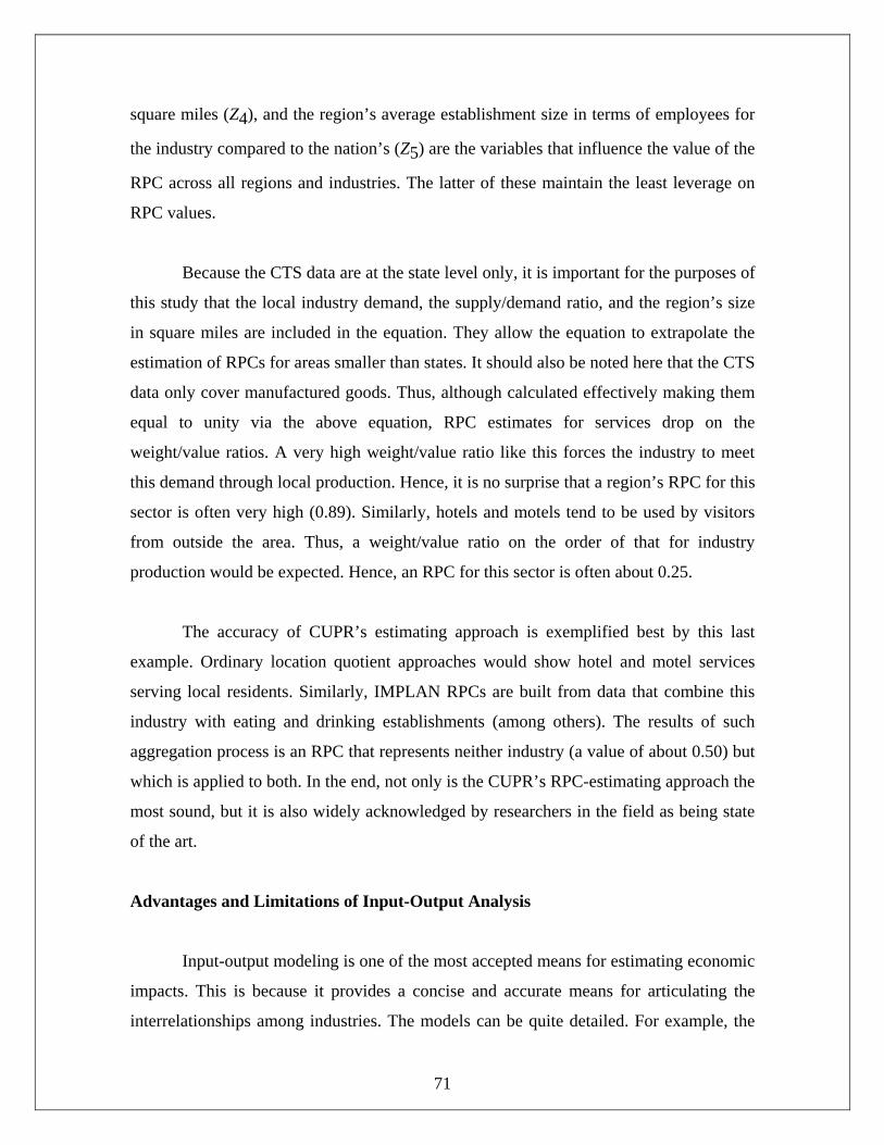
71
square miles (Z4), and the region’s average establishment size in terms of employees for
the industry compared to the nation’s (Z5) are the variables that influence the value of the
RPC across all regions and industries. The latter of these maintain the least leverage on
RPC values.
Because the CTS data are at the state level only, it is important for the purposes of
this study that the local industry demand, the supply/demand ratio, and the region’s size
in square miles are included in the equation. They allow the equation to extrapolate the
estimation of RPCs for areas smaller than states. It should also be noted here that the CTS
data only cover manufactured goods. Thus, although calculated effectively making them
equal to unity via the above equation, RPC estimates for services drop on the
weight/value ratios. A very high weight/value ratio like this forces the industry to meet
this demand through local production. Hence, it is no surprise that a region’s RPC for this
sector is often very high (0.89). Similarly, hotels and motels tend to be used by visitors
from outside the area. Thus, a weight/value ratio on the order of that for industry
production would be expected. Hence, an RPC for this sector is often about 0.25.
The accuracy of CUPR’s estimating approach is exemplified best by this last
example. Ordinary location quotient approaches would show hotel and motel services
serving local residents. Similarly, IMPLAN RPCs are built from data that combine this
industry with eating and drinking establishments (among others). The results of such
aggregation process is an RPC that represents neither industry (a value of about 0.50) but
which is applied to both. In the end, not only is the CUPR’s RPC-estimating approach the
most sound, but it is also widely acknowledged by researchers in the field as being state
of the art.
Advantages and Limitations of Input-Output Analysis
Input-output modeling is one of the most accepted means for estimating economic
impacts. This is because it provides a concise and accurate means for articulating the
interrelationships among industries. The models can be quite detailed. For example, the

72
current U.S. model currently has more than 500 industries representing many six-digit
North American Industrial Classification System (NAICS) codes. The CUPR’s model
used in this study has 517 sectors. Further, the industry detail of input-output models
provides not only a consistent and systematic approach but also more accurately assesses
multiplier effects of changes in economic activity. Research has shown that results from
more aggregated economic models can have as much as 50 percent error inherent in
them. Such large errors are generally attributed to poor estimation of regional trade flows
resulting from the aggregation process.
Input-output models also can be set up to capture the flows among economic
regions. For example, the model used in this study can calculate impacts for a county as
well as the total New Jersey state economy.
The limitations of input-output modeling should also be recognized. The approach
makes several key assumptions. First, the input-output model approach assumes that
there are no economies of scale to production in an industry; that is, the proportion of
inputs used in an industry’s production process does not change regardless of the level of
production. This assumption will not work if the technology matrix depicts an economy
of a recessional economy (e.g., 1982) and the analyst is attempting to model activity in a
peak economic year (e.g., 1989). In a recession year, the labor-to-output ratio tends to be
excessive because firms are generally reluctant to lay off workers when they believe an
economic turnaround is about to occur.
A less-restrictive assumption of the input-output approach is that technology is
not permitted to change over time. It is less restrictive because the technology matrix in
the United States is updated frequently and, in general, production technology does not
radically change over short periods.
Finally, the technical coefficients used in most regional models are based on the
assumption that production processes are spatially invariant and are well represented by

73
the nation’s average technology. In a region as large and diverse as New Jersey, this
assumption is likely to hold true.
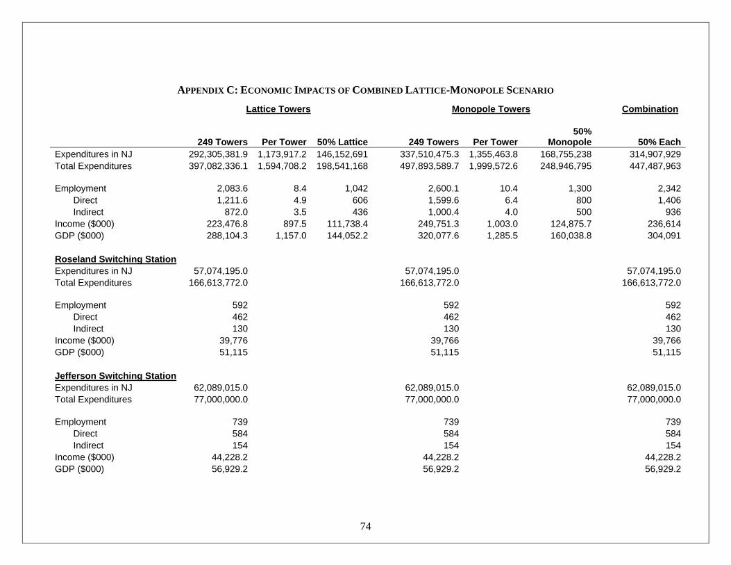
74
APPENDIX C: ECONOMIC IMPACTS OF COMBINED LATTICE-MONOPOLE SCENARIO
Lattice Towers Monopole Towers Combination
249 Towers Per Tower 50% Lattice 249 Towers Per Tower50%
Monopole 50% Each Expenditures in NJ 292,305,381.9 1,173,917.2 146,152,691 337,510,475.3 1,355,463.8 168,755,238 314,907,929 Total Expenditures 397,082,336.1 1,594,708.2 198,541,168 497,893,589.7 1,999,572.6 248,946,795 447,487,963 Employment 2,083.6 8.4 1,042 2,600.1 10.4 1,300 2,342
Direct 1,211.6 4.9 606 1,599.6 6.4 800 1,406 Indirect 872.0 3.5 436 1,000.4 4.0 500 936
Income ($000) 223,476.8 897.5 111,738.4 249,751.3 1,003.0 124,875.7 236,614 GDP ($000) 288,104.3 1,157.0 144,052.2 320,077.6 1,285.5 160,038.8 304,091 Roseland Switching Station Expenditures in NJ 57,074,195.0 57,074,195.0 57,074,195.0 Total Expenditures 166,613,772.0 166,613,772.0 166,613,772.0 Employment 592 592 592
Direct 462 462 462 Indirect 130 130 130
Income ($000) 39,776 39,766 39,766 GDP ($000) 51,115 51,115 51,115 Jefferson Switching Station Expenditures in NJ 62,089,015.0 62,089,015.0 62,089,015.0 Total Expenditures 77,000,000.0 77,000,000.0 77,000,000.0 Employment 739 739 739
Direct 584 584 584 Indirect 154 154 154
Income ($000) 44,228.2 44,228.2 44,228.2 GDP ($000) 56,929.2 56,929.2 56,929.2
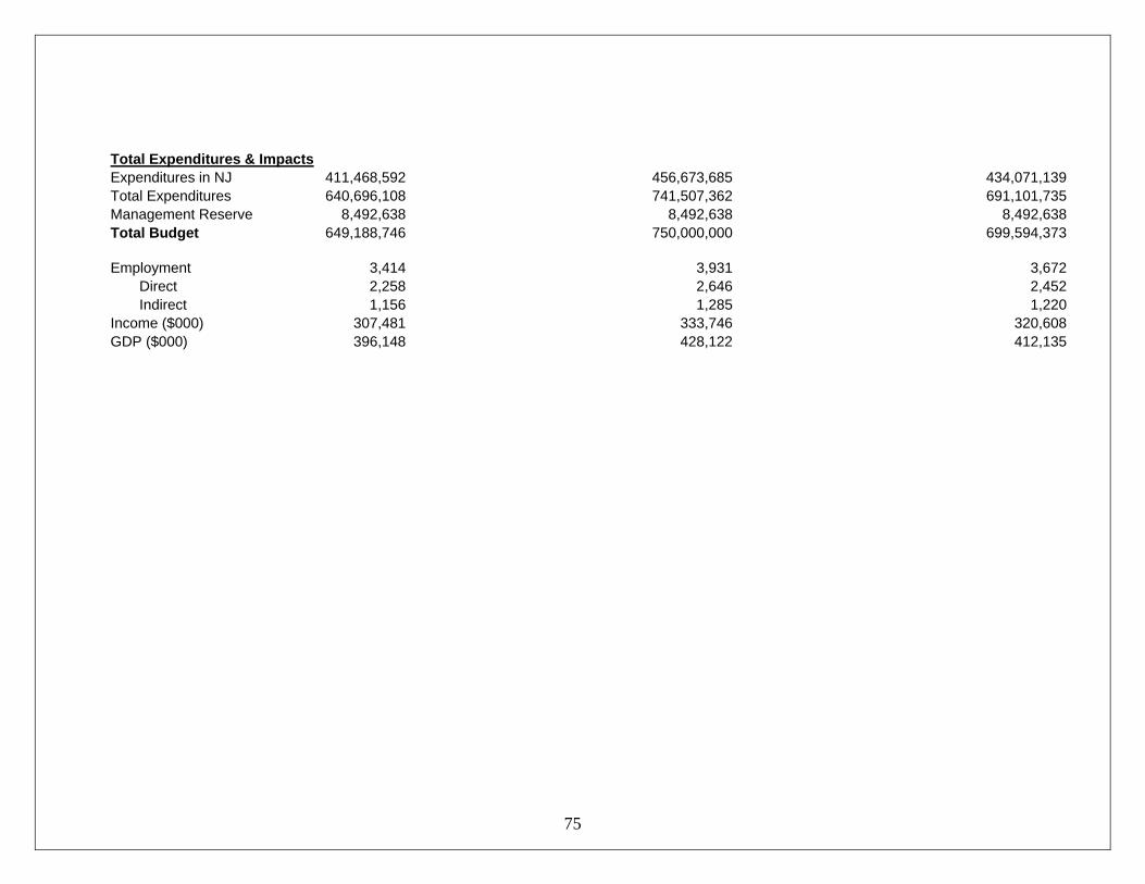
75
Total Expenditures & Impacts Expenditures in NJ 411,468,592 456,673,685 434,071,139 Total Expenditures 640,696,108 741,507,362 691,101,735 Management Reserve 8,492,638 8,492,638 8,492,638 Total Budget 649,188,746 750,000,000 699,594,373 Employment 3,414 3,931 3,672
Direct 2,258 2,646 2,452 Indirect 1,156 1,285 1,220
Income ($000) 307,481 333,746 320,608 GDP ($000) 396,148 428,122 412,135
Recommended