S. Parsons, R. Evans and M. Hoban
September 2008
Surface–groundwater connectivity assessmentA report to the Australian Government from the
CSIRO Murray-Darling Basin Sustainable Yields Project

Murray-Darling Basin Sustainable Yields Project acknowledgments
The Murray-Darling Basin Sustainable Yields project is being undertaken by CSIRO under the Australian Government's Raising National
Water Standards Program, administered by the National Water Commission. Important aspects of the work were undertaken by Sinclair
Knight Merz; Resource & Environmental Management Pty Ltd; Department of Water and Energy (New South Wales); Department of
Natural Resources and Water (Queensland); Murray-Darling Basin Commission; Department of Water, Land and Biodiversity
Conservation (South Australia); Bureau of Rural Sciences; Salient Solutions Australia Pty Ltd; eWater Cooperative Research Centre;
University of Melbourne; Webb, McKeown and Associates Pty Ltd; and several individual sub-contractors.
Murray-Darling Basin Sustainable Yields Project disclaimers
Derived from or contains data and/or software provided by the Organisations. The Organisations give no warranty in relation to the data
and/or software they provided (including accuracy, reliability, completeness, currency or suitability) and accept no liability (including
without limitation, liability in negligence) for any loss, damage or costs (including consequential damage) relating to any use or reliance
on that data or software including any material derived from that data and software. Data must not be used for direct marketing or be
used in breach of the privacy laws. Organisations include: Department of Water, Land and Biodiversity Conservation (South Australia),
Department of Sustainability and Environment (Victoria), Department of Water and Energy (New South Wales), Department of Natural
Resources and Water (Queensland), Murray-Darling Basin Commission.
CSIRO advises that the information contained in this publication comprises general statements based on scientific research. The reader
is advised and needs to be aware that such information may be incomplete or unable to be used in any specific situation. No reliance or
actions must therefore be made on that information without seeking prior expert professional, scientific and technical advice. To the
extent permitted by law, CSIRO (including its employees and consultants) excludes all liability to any person for any consequences,
including but not limited to all losses, damages, costs, expenses and any other compensation, arising directly or indirectly from using
this publication (in part or in whole) and any information or material contained in it. Data is assumed to be correct as received from the
Organisations.
Acknowledgements
Lauren Helm, Eliza Wiltshire, Michael Hoban and Ann Kollmorgen were involved in development of various connectivity maps for each
of the regions.
Citation
Parsons S, Evans R and Hoban M (2008) Surface–groundwater connectivity assessment. A report to the Australian Government from
the CSIRO Murray-Darling Basin Sustainable Yields Project. CSIRO, Australia. 35pp.
Publication Details
Published by CSIRO © 2008 all rights reserved. This work is copyright. Apart from any use as permitted under the Copyright Act 1968,
no part may be reproduced by any process without prior written permission from CSIRO.
ISSN 1835-095X

Preface
This is a report to the Australian Government from CSIRO. It is an output of the Murray-Darling Basin Sustainable Yields
Project which assessed current and potential future water availability in 18 regions across the Murray-Darling Basin
(MDB) considering climate change and other risks to water resources. The project was commissioned following the
Murray-Darling Basin Water Summit convened by the then Prime Minister of Australia in November 2006 to report
progressively during the latter half of 2007. The reports for each of the 18 regions and for the entire MDB are supported
by a series of technical reports detailing the modelling and assessment methods used in the project. This report is one of
the supporting technical reports of the project. Project reports can be accessed at http://www.csiro.au/mdbsy.
Project findings are expected to inform the establishment of a new sustainable diversion limit for surface and
groundwater in the MDB – one of the responsibilities of a new Murray-Darling Basin Authority in formulating a new
Murray-Darling Basin Plan, as required under the Commonwealth Water Act 2007. These reforms are a component of
the Australian Government’s new national water plan ‘Water for our Future’. Amongst other objectives, the national water
plan seeks to (i) address over-allocation in the MDB, helping to put it back on a sustainable track, significantly improving
the health of rivers and wetlands of the MDB and bringing substantial benefits to irrigators and the community; and (ii)
facilitate the modernisation of Australian irrigation, helping to put it on a more sustainable footing against the background
of declining water resources.
Executive Summary
Background
An important focus of the Murray-Darling Basin Sustainable Yields Project is proper accounting of surface–groundwater
interactions. This document provides an overview of the surface–groundwater connectivity assessment conducted for
this project. The connectivity assessment provides mapping information that links surface water (rivers) and groundwater
resources. Understanding the extent of interaction is important, as management of these two resources should take into
account the interconnection of the two systems. The connectivity mapping is a snapshot in time of fluxes to or from major
rivers across the Murray-Darling Basin (MDB). It can serve as a check for the surface water modelling and groundwater
modelling components of the project, which modelled the temporal dynamics of river–aquifer interactions. Further, areas
subject to groundwater modelling represent a relatively small portion of the MDB (albeit a high proportion of groundwater
usage), and therefore the connectivity mapping, covering 13 of the 18 regions in the project area, provides river–aquifer
interaction information across most of the MDB.
The connectivity mapping involved determining the direction and magnitude of groundwater flux to or from major rivers
for most catchments within the project area, for a given point in time. The regions where connectivity mapping was
conducted were: Loddon-Avoca, Campaspe, Goulburn-Broken, Ovens, Murray, Murrumbidgee, Lachlan, Macquarie-
Castlereagh, Namoi, Gwydir, Border Rivers, Condamine-Balonne and Barwon-Darling. The individual connectivity
mapping reports are specifically focused on the results within each catchment. The purpose of this overview report is to
describe the ‘big picture’ findings arising from the connectivity mapping.
While only representing a ‘snapshot in time’ of surface–groundwater interaction, the connectivity maps nevertheless
serve multiple purposes:
• They provide an alternate approach (to the numerical models) to assessing surface–groundwater interactions
across the MDB. This alternate methodology has some advantages over the numerical modelling, as discussed
in this report.
• They serve as a check of the surface water modelling and groundwater modelling components of the project.
• They provide an initial (and sometimes rapid) assessment that can be used as the basis for more detailed
conceptualisation as part of modelling.
• They estimate interactions outside of the modelled areas, which represent a relatively small part of the MDB.
© CSIRO 2008 Surface–groundwater connectivity assessment
• They are a powerful visual aid, with significant communication and education value. A map is an ideal tool for
initiating discussions and catalysing questions regarding surface–groundwater interactions. While the maps may
be shown to be locally inaccurate compared to future work undertaken at a finer scale, they nevertheless serve
a very useful purpose as a starting point for conceptualising surface–groundwater interactions.
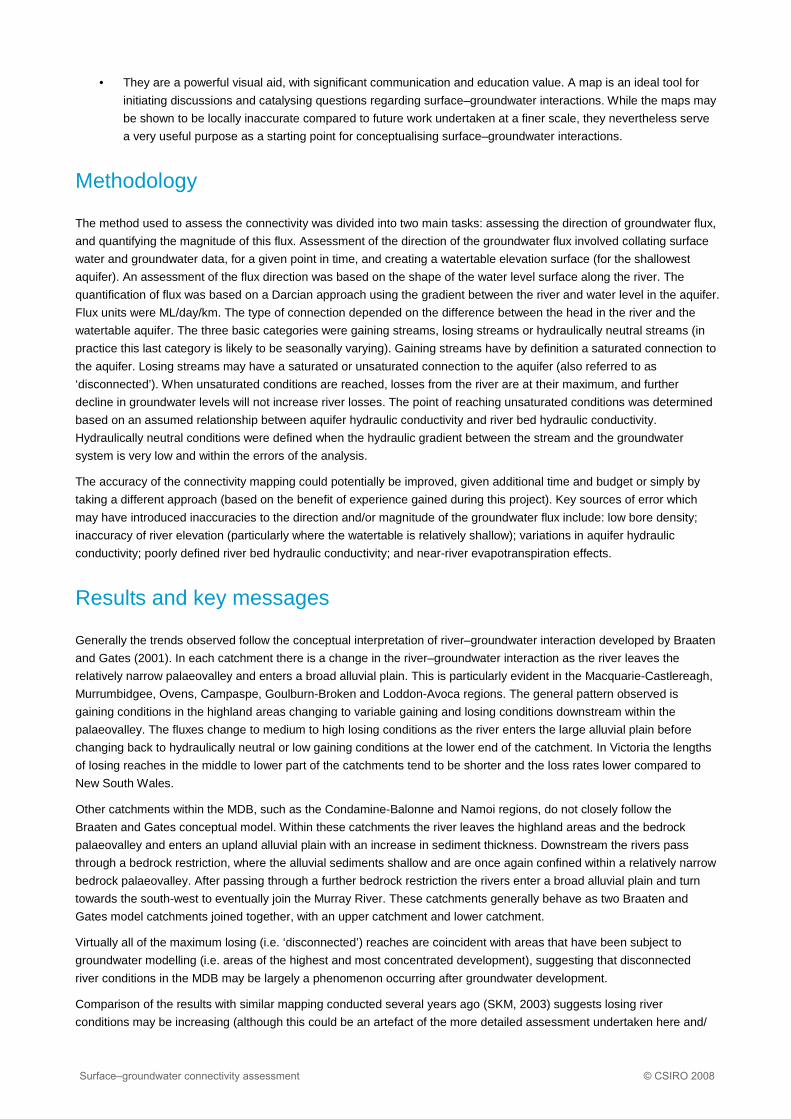
Methodology
The method used to assess the connectivity was divided into two main tasks: assessing the direction of groundwater flux,
and quantifying the magnitude of this flux. Assessment of the direction of the groundwater flux involved collating surface
water and groundwater data, for a given point in time, and creating a watertable elevation surface (for the shallowest
aquifer). An assessment of the flux direction was based on the shape of the water level surface along the river. The
quantification of flux was based on a Darcian approach using the gradient between the river and water level in the aquifer.
Flux units were ML/day/km. The type of connection depended on the difference between the head in the river and the
watertable aquifer. The three basic categories were gaining streams, losing streams or hydraulically neutral streams (in
practice this last category is likely to be seasonally varying). Gaining streams have by definition a saturated connection to
the aquifer. Losing streams may have a saturated or unsaturated connection to the aquifer (also referred to as
‘disconnected’). When unsaturated conditions are reached, losses from the river are at their maximum, and further
decline in groundwater levels will not increase river losses. The point of reaching unsaturated conditions was determined
based on an assumed relationship between aquifer hydraulic conductivity and river bed hydraulic conductivity.
Hydraulically neutral conditions were defined when the hydraulic gradient between the stream and the groundwater
system is very low and within the errors of the analysis.
The accuracy of the connectivity mapping could potentially be improved, given additional time and budget or simply by
taking a different approach (based on the benefit of experience gained during this project). Key sources of error which
may have introduced inaccuracies to the direction and/or magnitude of the groundwater flux include: low bore density;
inaccuracy of river elevation (particularly where the watertable is relatively shallow); variations in aquifer hydraulic
conductivity; poorly defined river bed hydraulic conductivity; and near-river evapotranspiration effects.
Results and key messages
Generally the trends observed follow the conceptual interpretation of river–groundwater interaction developed by Braaten
and Gates (2001). In each catchment there is a change in the river–groundwater interaction as the river leaves the
relatively narrow palaeovalley and enters a broad alluvial plain. This is particularly evident in the Macquarie-Castlereagh,
Murrumbidgee, Ovens, Campaspe, Goulburn-Broken and Loddon-Avoca regions. The general pattern observed is
gaining conditions in the highland areas changing to variable gaining and losing conditions downstream within the
palaeovalley. The fluxes change to medium to high losing conditions as the river enters the large alluvial plain before
changing back to hydraulically neutral or low gaining conditions at the lower end of the catchment. In Victoria the lengths
of losing reaches in the middle to lower part of the catchments tend to be shorter and the loss rates lower compared to
New South Wales.
Other catchments within the MDB, such as the Condamine-Balonne and Namoi regions, do not closely follow the
Braaten and Gates conceptual model. Within these catchments the river leaves the highland areas and the bedrock
palaeovalley and enters an upland alluvial plain with an increase in sediment thickness. Downstream the rivers pass
through a bedrock restriction, where the alluvial sediments shallow and are once again confined within a relatively narrow
bedrock palaeovalley. After passing through a further bedrock restriction the rivers enter a broad alluvial plain and turn
towards the south-west to eventually join the Murray River. These catchments generally behave as two Braaten and
Gates model catchments joined together, with an upper catchment and lower catchment.
Virtually all of the maximum losing (i.e. ‘disconnected’) reaches are coincident with areas that have been subject to
groundwater modelling (i.e. areas of the highest and most concentrated development), suggesting that disconnected
river conditions in the MDB may be largely a phenomenon occurring after groundwater development.
Comparison of the results with similar mapping conducted several years ago (SKM, 2003) suggests losing river
conditions may be increasing (although this could be an artefact of the more detailed assessment undertaken here and/
Surface–groundwater connectivity assessment © CSIRO 2008

or the much drier conditions at the time of this analysis). Nevertheless, it is likely that river losses may become greater
and river gains become further reduced into the future (in particular on the broad alluvial plains) as groundwater systems
begin to fully reflect changing climatic conditions, time lags from groundwater development are realised, and
groundwater extraction increases in some areas. Identifying the impacts of groundwater development on rivers and the
processes behind river–aquifer interaction will therefore become even more important if water management is to move
towards a truly integrated approach.
© CSIRO 2008 Surface–groundwater connectivity assessment

Table of Contents
1 Introduction............................................................................................................................... 1
2 Method overview ..................................................................................................................... 3 2.1 Connectivity mapping ...................................................................................................................................................3 2.2 Quantification of flux.....................................................................................................................................................5
3 Lessons learnt............................................................................................................................ 9
4 Overview of accuracy of maps............................................................................................ 13 4.1 Likely inaccuracies .....................................................................................................................................................13
4.1.1 Flux direction................................................................................................................................................13 4.1.2 Flux magnitude.............................................................................................................................................13
4.2 Comparison with numerical model..............................................................................................................................14
5 MDB-wide interpretation........................................................................................................ 16 5.1 Trends and processes................................................................................................................................................16 5.2 Future trends..............................................................................................................................................................18 5.3 Implications and future work .......................................................................................................................................19
References .............................................................................................................................................. 20
Appendix A Regional surface–groundwater connectivity maps ............................................... 21
Tables
Table 2-1. Assessment dates for connectivity mapping....................................................................................................................4
Figures
Figure 2-1. Theoretical relationship between clogging layer hydraulic conductivity and stream width / depth to watertable (after Rassam, 2008) ................................................................................................................................................................................7 Figure 3-1. Example of impact of different methods of interpolating between river elevations ..........................................................9 Figure 5-1. Surface–groundwater connectivity map across the Murray-Darling Basin ....................................................................16 Figure 5-2. Surface–groundwater connectivity for the Barwon-Darling region ................................................................................21 Figure 5-3. Surface–groundwater connectivity for the Border Rivers region ...................................................................................22 Figure 5-4. Surface–groundwater connectivity for the Campaspe region........................................................................................23 Figure 5-5. Surface–groundwater connectivity for the Condamine region.......................................................................................24 Figure 5-6. Surface–groundwater connectivity for the Goulburn-Broken region..............................................................................25 Figure 5-7. Surface–groundwater connectivity for the Gwydir region..............................................................................................26 Figure 5-8. Surface–groundwater connectivity for the Lachlan region ............................................................................................27 Figure 5-9. Surface–groundwater connectivity for the Loddon-Avoca region..................................................................................28 Figure 5-10. Surface–groundwater connectivity for the Macquarie-Castlereagh region ..................................................................29 Figure 5-11. Surface–groundwater connectivity for the Murrumbidgee region ................................................................................30 Figure 5-12. Surface–groundwater connectivity for the Murray region............................................................................................31 Figure 5-13. Surface–groundwater connectivity for the Namoi region.............................................................................................32 Figure 5-14. Surface–groundwater connectivity for the Ovens region.............................................................................................33
Surface–groundwater connectivity assessment © CSIRO 2008
1 Introduction
An important focus of the Murray-Darling Basin Sustainable Yields Project is proper accounting of surface–groundwater
interactions. This document provides an overview of surface–groundwater connectivity mapping conducted for this
project. Historically, these two resources have largely been managed as separate systems, despite the physical reality of
their interconnection. The implication of this management has been ‘double accounting’ whereby the same parcel of
water may be allocated to both surface water users and to groundwater users. The extent of ‘double accounting’
throughout the MDB is not well known, and similarly the nature of interactions between groundwater and surface water
are poorly understood.
A first step in understanding fundamental processes is knowledge of basic interactions between rivers and groundwater.
The relationship at its most basic reduces to the question: is the river losing or gaining groundwater and at what rate? It
is this basic interaction which the connectivity assessment aimed to identify and map. In practice such interactions are
dynamic, fluctuating both seasonally and over the long term in response to climatic changes and the delayed impact of
groundwater extractions. Hence the connectivity maps presented in this report only represent a ‘snapshot in time’ of the
current state of interactions. It is therefore important to note when using these maps that the impact of a significant
portion of groundwater development is not yet reflected in the results (i.e. into the future we can expect gaining streams
to be gaining at a lower rate and losing streams to be losing at a higher rate as delayed impacts are realised, assuming
current climatic conditions continue).
In addition to these connectivity maps, numerical groundwater modelling has also been undertaken as part of this project
for high priority areas (defined as areas with either high groundwater usage or high potential to impact on streams). The
numerical modelling has identified the dynamic nature and extent of surface–groundwater interactions for these areas,
and has enabled prediction of changes in this interaction into the future. The numerical groundwater modelling was in
turn fed into surface water models in order to account for interaction between the two systems. The results of the
modelling are recorded in individual reports for the high priority areas. A summary of the methods adopted, lessons
learnt and recommendations arising from the numerical groundwater modelling, particularly relating to the surface–
groundwater interaction aspects of the modelling, is provided in Rassam (2008).
While only representing a ‘snapshot in time’ of surface–groundwater interaction, the connectivity maps nevertheless
serve multiple purposes:
• They provide an alternate approach (to the numerical models) to assessing surface–groundwater interactions
across the MDB. The alternate methodology has some advantages over the numerical modelling, as discussed
in this report.
• They serve as a check of the surface water modelling and groundwater modelling components of the project.
• They provide an initial (and sometimes rapid) assessment that can be used as the basis for more detailed
conceptualisation as part of modelling.
• They estimate interactions outside of the modelled areas.
• They are a powerful visual aid, with significant communication and education value. A map is an ideal tool for
initiating discussions and catalysing questions regarding surface–groundwater interactions. While the maps may
be shown to be inaccurate compared to current or future work undertaken at a finer scale, they nevertheless
serve a very useful purpose as a starting point for conceptualising surface–groundwater interactions.
Given the many uses of the maps, it is anticipated that these maps will be of interest and value to water resource
managers and related professionals across the MDB, in that they provide a valuable starting point in understanding
stream–aquifer interaction, and in turn how groundwater management may impact on the riverine environment and
groundwater-dependent ecosystems.
The connectivity mapping involved determining the direction and magnitude of groundwater flux to or from the major
rivers within 13 of the 18 regions of the MDB for a given point in time (between March 2005 and June 2006). The regions
where connectivity mapping was conducted were: Loddon-Avoca, Campaspe, Goulburn-Broken, Ovens, Murray,
Murrumbidgee, Lachlan, Macquarie-Castlereagh, Namoi, Gwydir, Border Rivers, Condamine-Balonne and Barwon-
Darling. For each of these catchments a stand-alone connectivity report has been prepared. These individual reports
describe in detail the connectivity mapping results for each catchment. They also contain a stand-alone map for each
catchment, which is also reproduced in this report. The assessment and analysis in the individual connectivity reports
© CSIRO 2008 Surface–groundwater connectivity assessment ▪ 1

were specifically focused on the results within each catchment. The purpose of this overview report is to describe the ‘big
picture’ findings arising from the connectivity mapping. The aim of each section of the report is described below:
• Method overview – This section summarises the methodology adopted in the connectivity mapping.
• Lessons learnt – The objective of this section is to describe key areas where lessons were learnt within the
connectivity mapping process, and to discuss how the task could be undertaken better or more efficiently in the
future.
• Overview of accuracy of maps – The aim of this section is to provide an indication of the reliability of the maps.
The question considered is ‘How accurate do we believe the maps are?’
• MDB-wide interpretation – This section provides an overview of trends and observations across all the
connectivity maps. A MDB-wide connectivity map is presented. This map links results from all 13 catchments
where connectivity mapping was undertaken.
2 ▪ Surface–groundwater connectivity assessment © CSIRO 2008

2 Method overview
This section describes the method used to assess the connectivity. The method is divided into two main tasks: firstly,
assess the direction of groundwater flux (referred to here as ‘connectivity mapping’) and secondly, quantify the
magnitude of this flux. For each of these tasks, the major steps involved in the process are described.
2.1 Connectivity mapping
1. River reach selection
The issues that were considered in selecting the rivers or river reaches to include in the connectivity assessment
were:
• ‘Main’ river/s – there was typically one, and often two or three rivers, that were clearly the main rivers within the
catchment and hence required assessment.
• Groundwater modelled areas – rivers included in a groundwater modelled area were included in the
assessment.
• Other ‘representative’ river reaches – these were included where there was a need to map a river or part of a
river in order to demonstrate conceptual understanding in that part of the catchment, e.g. picking one reach in
highland areas to show understanding of processes in upland areas.
• Catchment-specific issues – rivers or reaches might be assessed due to catchment-specific issues which
increase interest in that area.
• Surface water modelled areas – rivers included in surface water modelling were generally included in the
assessment, i.e. reaches covered by IQQM / REALM models.
• Definition of rivers – in addition to perennial rivers, major ephemeral rivers within each catchment were also
included. A precise definition of what constituted an ephemeral river was not applied in the selection process.
Generally, however, a ‘major’ ephemeral river was considered to be one which flowed for more than just a few
weeks of the year (i.e. at least a couple of months), and secondly one that contributed a reasonable percentage
of total annual flow in the catchment.
2. Identify groundwater model stream gauge sites
Data was collated from the groundwater model stream gauges and any other intermediate gauges or gauges
representing reaches included in the connectivity assessment, but not in the groundwater model.
3. Date selection
A date was selected for the mapping and flux assessment. A date as close to current as possible was selected (e.g.
2005/06) as the aim of the task was to assess existing developed conditions (ignoring time lags). However the
selected date was sometimes constrained by the availability of surface water or groundwater elevation data. The
date was also selected so as to exclude any unrepresentative peaks or troughs in the data (i.e. dates with relatively
stable river and groundwater levels were chosen). High flow events in the rivers were avoided, as low river flows are
more common. It is important to note that ‘date’ actually refers to a span of several months (e.g. February to April
2005) because groundwater levels are not available for all bores within a catchment on a single date. Rather than
infilling data to obtain a level for a given date, a value was obtained by selecting the closest date to the target date
(one month either side of the target month). (In two catchments, Ovens and Border Rivers, up to four months either
side of the selected date was allowed but this only applied to a relatively small percentage of bores within those
catchments.) The date selected for the assessment of each catchment is shown in Table 2-1.
© CSIRO 2008 Surface–groundwater connectivity assessment ▪ 3
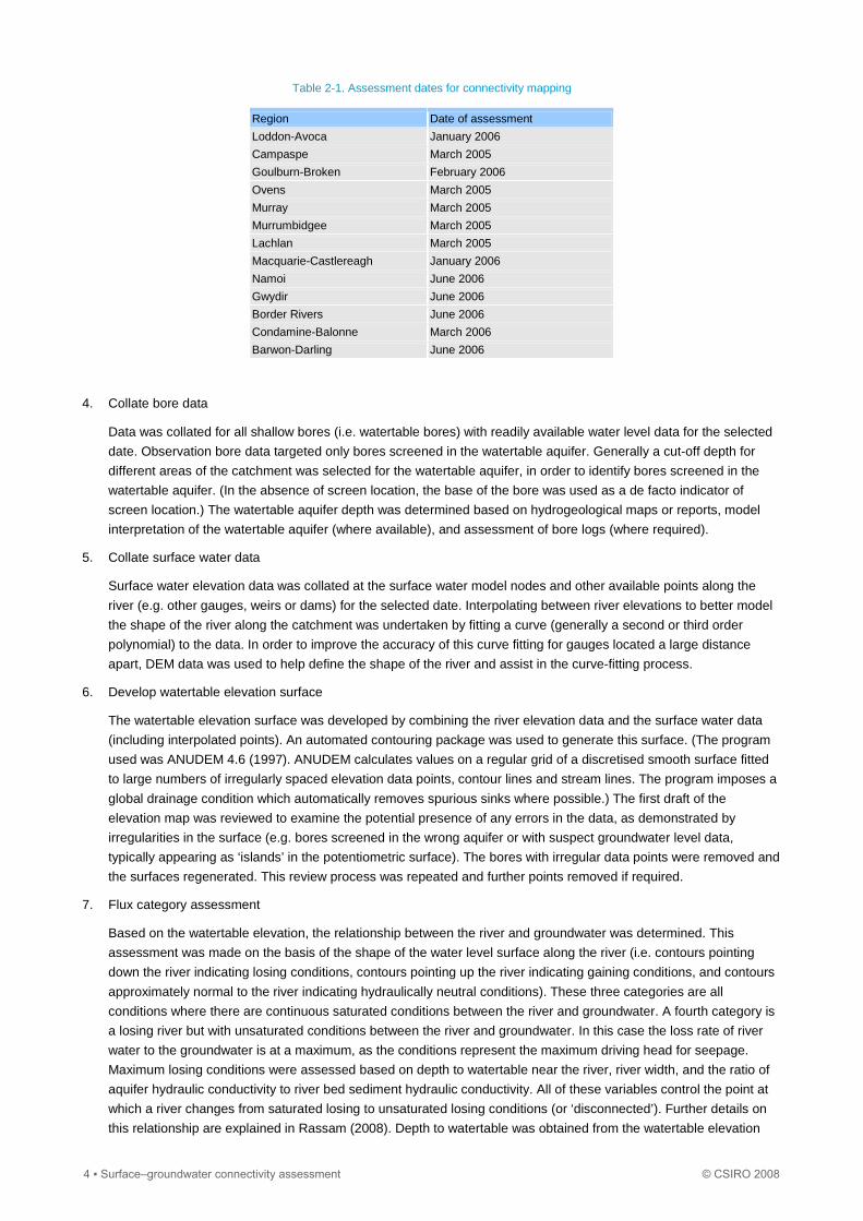
Table 2-1. Assessment dates for connectivity mapping
Region Date of assessment
Loddon-Avoca January 2006
Campaspe March 2005
Goulburn-Broken February 2006
Ovens March 2005
Murray March 2005
Murrumbidgee March 2005
Lachlan March 2005
Macquarie-Castlereagh January 2006
Namoi June 2006
Gwydir June 2006
Border Rivers June 2006
Condamine-Balonne March 2006
Barwon-Darling June 2006
4. Collate bore data
Data was collated for all shallow bores (i.e. watertable bores) with readily available water level data for the selected
date. Observation bore data targeted only bores screened in the watertable aquifer. Generally a cut-off depth for
different areas of the catchment was selected for the watertable aquifer, in order to identify bores screened in the
watertable aquifer. (In the absence of screen location, the base of the bore was used as a de facto indicator of
screen location.) The watertable aquifer depth was determined based on hydrogeological maps or reports, model
interpretation of the watertable aquifer (where available), and assessment of bore logs (where required).
5. Collate surface water data
Surface water elevation data was collated at the surface water model nodes and other available points along the
river (e.g. other gauges, weirs or dams) for the selected date. Interpolating between river elevations to better model
the shape of the river along the catchment was undertaken by fitting a curve (generally a second or third order
polynomial) to the data. In order to improve the accuracy of this curve fitting for gauges located a large distance
apart, DEM data was used to help define the shape of the river and assist in the curve-fitting process.
6. Develop watertable elevation surface
The watertable elevation surface was developed by combining the river elevation data and the surface water data
(including interpolated points). An automated contouring package was used to generate this surface. (The program
used was ANUDEM 4.6 (1997). ANUDEM calculates values on a regular grid of a discretised smooth surface fitted
to large numbers of irregularly spaced elevation data points, contour lines and stream lines. The program imposes a
global drainage condition which automatically removes spurious sinks where possible.) The first draft of the
elevation map was reviewed to examine the potential presence of any errors in the data, as demonstrated by
irregularities in the surface (e.g. bores screened in the wrong aquifer or with suspect groundwater level data,
typically appearing as ‘islands’ in the potentiometric surface). The bores with irregular data points were removed and
the surfaces regenerated. This review process was repeated and further points removed if required.
7. Flux category assessment
Based on the watertable elevation, the relationship between the river and groundwater was determined. This
assessment was made on the basis of the shape of the water level surface along the river (i.e. contours pointing
down the river indicating losing conditions, contours pointing up the river indicating gaining conditions, and contours
approximately normal to the river indicating hydraulically neutral conditions). These three categories are all
conditions where there are continuous saturated conditions between the river and groundwater. A fourth category is
a losing river but with unsaturated conditions between the river and groundwater. In this case the loss rate of river
water to the groundwater is at a maximum, as the conditions represent the maximum driving head for seepage.
Maximum losing conditions were assessed based on depth to watertable near the river, river width, and the ratio of
aquifer hydraulic conductivity to river bed sediment hydraulic conductivity. All of these variables control the point at
which a river changes from saturated losing to unsaturated losing conditions (or ‘disconnected’). Further details on
this relationship are explained in Rassam (2008). Depth to watertable was obtained from the watertable elevation
4 ▪ Surface–groundwater connectivity assessment © CSIRO 2008
map; river width was estimated from readily available satellite imagery; and aquifer hydraulic conductivity was
obtained from hydrogeological maps, reports and (where appropriate) values adopted in the groundwater models.
River bed hydraulic conductivity was assumed to be proportional to aquifer hydraulic conductivity (10% or 1% of
aquifer hydraulic conductivity).
In summary, the four categories used in the connectivity assessment are:
• A – gaining
• B – losing
• C – hydraulically neutral
• D – losing, unsaturated. (This condition represents the maximum loss rate for the given reach, described as
‘maximum losing’ or ‘disconnected’.)
Some important notes regarding these classifications are described below:
• Hydraulically neutral conditions are defined when the hydraulic gradient between the stream and the
groundwater system is very low and within the errors of the analysis. In a strictly technical sense it is not
possible to have a pure category C (hydraulically neutral condition), because in practice groundwater levels will
seasonally (and intra-seasonally) fluctuate, meaning that flux condition will change from losing to gaining across
the year. River levels will also go up and down, further adding to variability about this approximately neutral
condition. Hence, a system which is approximately hydraulically neutral at a point in time is most likely actually
one that is seasonally variable.
• Determining the difference between a stream that is losing and losing unsaturated may not be straightforward
with available data. The most important limiting factor will be determining with some level of accuracy the
hydraulic properties of the river bed material. Some rivers within the MDB will have information on river bed
materials, etc. However in many cases it may be difficult to obtain this information, and it certainly will be very
inconsistent across the mapped areas. (A detailed investigation of this was beyond the scope of the project.)
Further, whether flow from the river is unsaturated depends firstly on the depth to watertable below a losing
stream. When assessing this factor, a bore set too far away from the stream could over estimate the depth to
watertable near the stream and lead to a conclusion of unsaturated conditions. Bores close to the stream are
therefore preferred.
• A fifth category which could be added to the four above is ‘losing, variably saturated’ (i.e. seasonally changes
between category B and D in response to either natural groundwater fluctuations or enhanced groundwater
fluctuations resulting from river seepage). It was considered unrealistic at this level of assessment to expect to
be able to differentiate between category D and ‘losing, variably saturated’, so this latter category was not used.
• A final category that could have been added to the list is ‘through-flow rivers’, which are rivers where
groundwater flows into one side of the river and out of the other side. These are relatively uncommon in the
project area and hence no special category has been created for this type of river. They have been classified as
either ‘gaining’ or ‘losing’ according to their net flux into or out of the river.
• An additional temporal consideration is river reaches which display long-term changes between categories. This
is not possible to report in a classification system which captures a point in time, but if such changes were
observed from assessment of key hydrographs then a discussion of this was included in the report.
• Where data was not available for the classification, it was based on classical geomorphological/hydrogeological
interpretation, coupled with personal judgement in consultation with local experts.
• If the dominant flow process to or from the river were horizontal, an average near-river aquifer hydraulic
conductivity was assigned. If the dominant flow processes were vertical, the reach was attributed a conductance
based on the layer-thickness weighting (across the full thickness of any semi-confining layer). If no semi-
confining layer existed, then the vertical hydraulic conductivity of the aquifer was utilised.
2.2 Quantification of flux
This task involved estimating the magnitude of water flux between groundwater and surface water for the selected
assessment date. The calculation of the direction and magnitude of the flux (ML/day/km) was semi-automated via an
Excel spreadsheet using a Darcian approach.
© CSIRO 2008 Surface–groundwater connectivity assessment ▪ 5
Application of equation where horizontal flow processes are dominant
For river reaches where horizontal flow processes were deemed to be the dominant exchange mechanism with the river
(i.e. gaining streams or saturated losing streams), a Darcy calculation was undertaken based on the horizontal gradient
to/from the river. Consideration of the relevant distance at which to estimate a groundwater gradient to/from the river was
important. Selection of a relatively large distance over which the gradient was calculated (e.g. 1 to 2 km) provided a
longer term temporal averaging effect on the results, and was deemed more appropriate than a gradient based on data
close to the river which would reflect short-term groundwater–river dynamics. The relevant bulk average hydraulic
conductivity of the aquifer over the relevant distance and the applicable depth of aquifer contributing to exchange was
considered and documented.
Application of equation where vertical flow processes are dominant (unsaturated losing conditions)
For river reaches where vertical flow processes were dominant (i.e. unsaturated losing streams), a Darcian approach
assuming a linear relationship between river–groundwater head and flow rate would not have been valid (i.e. where the
watertable is deep and the river bed sediments have a lower hydraulic conductivity than the aquifer). In this instance the
stream loss rate will be at its maximum (i.e. ‘disconnected’), for the given river height. In these cases then either a
conductance term reflecting the thickness-weighted vertical hydraulic conductivity or more simply the aquifer vertical
hydraulic conductivity was used in the Darcy equation. The technically correct gradient to use is the head difference
between the river level and the pressure head in the river bed material, (determined from a mini-piezometer installed in
the stream bed), divided by the distance between the top of the river bed and the top of the mini-piezometer screen In
reality this gradient was not known (installation of mini-piezometers in the river bed layer are very rare), and therefore the
gradient was estimated. The maximum gradient is the head of water in the channel divided by the river bed layer
thickness; however this is considered likely to be an overestimate. In the absence of other information, a gradient of 1
was adopted. As described above, the relevant hydraulic conductivity in the equation was a thickness-weighted
conductance term, or in the absence of this (as was the case for the majority of reaches and catchments) the vertical
hydraulic conductivity of the aquifer was adopted as a de facto hydraulic conductivity of the river bed layer. In turn, the
vertical hydraulic conductivity of the aquifer was assumed to either 10% or 1% of horizontal hydraulic conductivity.
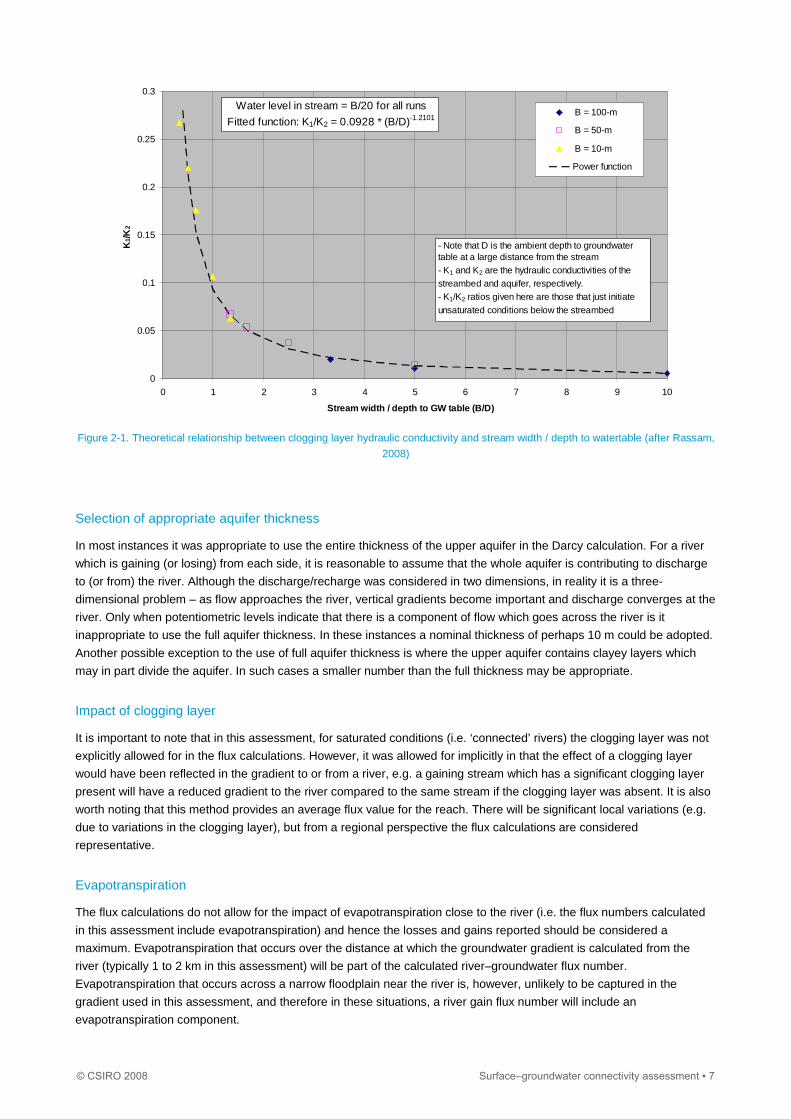
Determination of unsaturated losing conditions
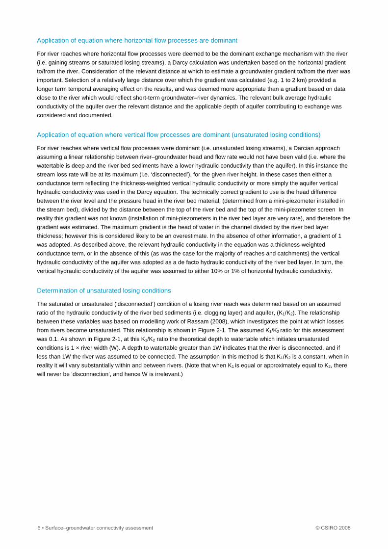
The saturated or unsaturated (‘disconnected’) condition of a losing river reach was determined based on an assumed
ratio of the hydraulic conductivity of the river bed sediments (i.e. clogging layer) and aquifer, (K1/K2). The relationship
between these variables was based on modelling work of Rassam (2008), which investigates the point at which losses
from rivers become unsaturated. This relationship is shown in Figure 2-1. The assumed K1/K2 ratio for this assessment
was 0.1. As shown in Figure 2-1, at this K1/K2 ratio the theoretical depth to watertable which initiates unsaturated
conditions is 1 × river width (W). A depth to watertable greater than 1W indicates that the river is disconnected, and if
less than 1W the river was assumed to be connected. The assumption in this method is that K1/K2 is a constant, when in
reality it will vary substantially within and between rivers. (Note that when K1 is equal or approximately equal to K2, there
will never be ‘disconnection’, and hence W is irrelevant.)
6 ▪ Surface–groundwater connectivity assessment © CSIRO 2008
0
0.05
0.1
0.15
0.2
0.25
0.3
0 1 2 3 4 5 6 7 8 9 10
Stream width / depth to GW table (B/D)
K1/
K2
B = 100-m
B = 50-m
B = 10-m
Power function
Water level in stream = B/20 for all runs
Fitted function: K1/K2 = 0.0928 * (B/D)-1.2101
- Note that D is the ambient depth to groundwater table at a large distance from the stream- K1 and K2 are the hydraulic conductivities of the streambed and aquifer, respectively.- K1/K2 ratios given here are those that just initiate unsaturated conditions below the streambed
Figure 2-1. Theoretical relationship between clogging layer hydraulic conductivity and stream width / depth to watertable (after Rassam,
2008)
Selection of appropriate aquifer thickness
In most instances it was appropriate to use the entire thickness of the upper aquifer in the Darcy calculation. For a river
which is gaining (or losing) from each side, it is reasonable to assume that the whole aquifer is contributing to discharge
to (or from) the river. Although the discharge/recharge was considered in two dimensions, in reality it is a three-
dimensional problem – as flow approaches the river, vertical gradients become important and discharge converges at the
river. Only when potentiometric levels indicate that there is a component of flow which goes across the river is it
inappropriate to use the full aquifer thickness. In these instances a nominal thickness of perhaps 10 m could be adopted.
Another possible exception to the use of full aquifer thickness is where the upper aquifer contains clayey layers which
may in part divide the aquifer. In such cases a smaller number than the full thickness may be appropriate.
Impact of clogging layer
It is important to note that in this assessment, for saturated conditions (i.e. ‘connected’ rivers) the clogging layer was not
explicitly allowed for in the flux calculations. However, it was allowed for implicitly in that the effect of a clogging layer
would have been reflected in the gradient to or from a river, e.g. a gaining stream which has a significant clogging layer
present will have a reduced gradient to the river compared to the same stream if the clogging layer was absent. It is also
worth noting that this method provides an average flux value for the reach. There will be significant local variations (e.g.
due to variations in the clogging layer), but from a regional perspective the flux calculations are considered
representative.
Evapotranspiration
The flux calculations do not allow for the impact of evapotranspiration close to the river (i.e. the flux numbers calculated
in this assessment include evapotranspiration) and hence the losses and gains reported should be considered a
maximum. Evapotranspiration that occurs over the distance at which the groundwater gradient is calculated from the
river (typically 1 to 2 km in this assessment) will be part of the calculated river–groundwater flux number.
Evapotranspiration that occurs across a narrow floodplain near the river is, however, unlikely to be captured in the
gradient used in this assessment, and therefore in these situations, a river gain flux number will include an
evapotranspiration component.
© CSIRO 2008 Surface–groundwater connectivity assessment ▪ 7

Uncertainty
The flux calculations contain uncertainty. Uncertainty is introduced at a number of levels including:
• estimates of aquifer parameters – in particular hydraulic conductivity, which can spatially vary markedly
• errors related to data density – for example, only a limited number of bores make up the potentiometric surface
and hence the surface contains inaccuracies related to extrapolation/interpolation of the surface, or estimates of
river stage may not be accurate due to the absence of gauges
• errors associated with assumptions in the method – for example, evapotranspiration close to the river is
assumed to be negligible; the method of determining saturated or unsaturated flow condition; and associated
assumptions regarding the clogging layer etc.
In some cases, uncertainties can be quantitatively determined. In this assessment, however, uncertainties were
discussed qualitatively and then based on understanding of the various uncertainties, different rivers or reaches were
assigned one of three uncertainty categories:
• A – high confidence
• B – moderate confidence
• C – low confidence.
Spatial variability
It is well documented that at the local scale, flux rates into or out of rivers can vary markedly within short distances due to
a high level of heterogeneity in near-river sediments. The calculations undertaken in this assessment did not attempt to
account for such local-scale processes. The flux values calculated represent average values for the mapped reaches.
The results of the flux calculations were tabulated for defined river reaches. Flux calculations were then compared with
groundwater modelling results.
8 ▪ Surface–groundwater connectivity assessment © CSIRO 2008
3 Lessons learnt
This section describes how the accuracy of the connectivity mapping could potentially be improved, given additional time
and budget or simply by taking a different approach, based on the benefit of experience gained during the exercise.
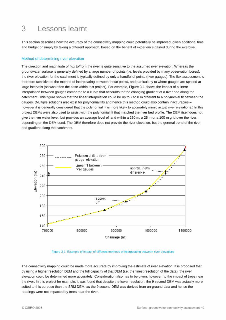
Method of determining river elevation
The direction and magnitude of flux to/from the river is quite sensitive to the assumed river elevation. Whereas the
groundwater surface is generally defined by a large number of points (i.e. levels provided by many observation bores),
the river elevation for the catchment is typically defined by only a handful of points (river gauges). The flux assessment is
therefore sensitive to the method of interpolating between these points, and particularly to where gauges are spaced at
large intervals (as was often the case within this project). For example, Figure 3-1 shows the impact of a linear
interpolation between gauges compared to a curve that accounts for the changing gradient of a river bed along the
catchment. This figure shows that the linear interpolation could be up to 7 to 8 m different to a polynomial fit between the
gauges. (Multiple solutions also exist for polynomial fits and hence this method could also contain inaccuracies –
however it is generally considered that the polynomial fit is more likely to accurately mimic actual river elevations.) In this
project DEMs were also used to assist with the polynomial fit that matched the river bed profile. The DEM itself does not
give the river water level, but provides an average level of land within a 250 m, a 25 m or a 100 m grid over the river,
depending on the DEM used. The DEM therefore does not provide the river elevation, but the general trend of the river
bed gradient along the catchment.
Figure 3-1. Example of impact of different methods of interpolating between river elevations
The connectivity mapping could be made more accurate by improving the estimate of river elevation. It is proposed that
by using a higher resolution DEM and the full capacity of that DEM (i.e. the finest resolution of the data), the river
elevation could be determined more accurately. Consideration also has to be given, however, to the impact of trees near
the river. In this project for example, it was found that despite the lower resolution, the 9 second DEM was actually more
suited to this purpose than the SRM DEM, as the 9 second DEM was derived from on-ground data and hence the
readings were not impacted by trees near the river.
© CSIRO 2008 Surface–groundwater connectivity assessment ▪ 9
Groundwater bore selection
• Date of selection
Selection of groundwater observation bores included in the connectivity mapping was limited to bores with
available groundwater levels either within the selected month, or one month either side of that month. In
hindsight, allowing greater flexibility around the selected month, to allow inclusion of more bores in the analysis,
would have been a better approach. This is because on the whole the temporal difference in groundwater levels
(even the maximum seasonal difference for a given bore) is typically fairly small, and generally less than the
error introduced by having no data present at all. Inclusion of groundwater levels up to 3 to 4 months either side
of the date (or even up to 2 to 3 years of the date) would have allowed inclusion of a larger number of
observation bores. Ideally, this method of bore selection would be a sophisticated method such that in areas
with high bore density, bores outside of the ideal date range (say within 1 to 2 months of the selected date)
would not be used, but in areas of low bore density, bores with data further from the selected date would be
used in the mapping.
• Use of other bore data to improve spatial coverage
Significant parts of the map were largely devoid of observation bore data. In such areas, watertable contours
were based on interpolation between very widely spaced observation bores. In order to improve the estimate of
the watertable surface in these areas, it is recommended that bores other than those readily available from the
state agency databases be used. This could include attempting to source information from other, ‘less official’
state groundwater databases (e.g. DPI in Victoria), the entirety of whose data may not be included on the main
state groundwater database. But more importantly this should involve inclusion of appropriate private bore data
(i.e. stock and domestic bores or irrigation bores) containing groundwater level information. (It is likely that
screen depths will need to be estimated from bore depth, and greater care would need to be exercised in bore
selection to avoid use of irrigation bore level data influenced by seasonal pumping.) While this data is clearly
unlikely to be as accurate as observation bore data, it is considered that use of such data in very data poor
areas would be much better.
Better method of determining 'disconnection'
One of the key areas for improvement in the mapping is development of a better method for determining areas of river
that are under maximum losing conditions (i.e. river and groundwater are separated from each other by an unsaturated
zone). In the method described in this report, a reach was determined to be disconnected based on an assumed ratio of
the hydraulic conductivity of the river bed sediments (i.e. clogging layer) and aquifer (K1/K2). The assumed K1/K2 ratio
for this assessment was 0.1. Based on the relationship shown in Figure 5-1, at this K1/K2 ratio the theoretical depth to
watertable which initiates unsaturated conditions is 1 × river width (W). The obvious problem with this assumption is that
K1/K2 varies substantially. In many stretches along rivers across the MDB it is likely that silt deposition means that K1/K2
could be substantially less than 0.1, meaning that unsaturated conditions will form at shallower depths than 1W. It is
therefore likely that the areas of ‘disconnected’ river have probably been under estimated using this method. However,
there are also likely to be some stretches of river where K1/K2 is greater than 0.1, which could have led to a
‘disconnected’ classification, when in fact they were connected.
A better method for more accurately estimating the K1/K2 ratio for major rivers in the MDB would improve the accuracy
of the connectivity mapping. Essentially this means development of a regional method of estimating river bed sediment
conductivity, as aquifer hydraulic conductivity is relatively well known. For example, river slope might be a reasonable
explanatory variable for the river bed sediment hydraulic conductivity, on the basis that slope relates to river velocity
which relates to the degree of sediment deposition (or perhaps better than slope, slope and cross-sectional area, or
slope and soil type). Clearly some reasonable basin-wide data on river bed properties would be required in order to
develop and calibrate such a relationship. As a minimum this would need to describe river bed material and thickness,
but ideally would include some conductivity measurements in the river bed sediments. It is probably unlikely that
sufficient data exists across the MDB in order to development a MDB-wide relationship between these variables.
Possibly a theoretical relationship could be established on the basis of geomorphological principles. If such a relationship
could be established then a K1/K2 ratio could be assigned to each river length using a GIS function.
Remote sensing should also then be applied in order to determine river width as close as possible to the assessment
date (or for similar level of flow if a suitable close date cannot be obtained). The method of estimating stream width in this
assessment was relatively crude and generally determined via a visual interpretation of the Google Earth satellite
10 ▪ Surface–groundwater connectivity assessment © CSIRO 2008

imagery and not as accurate as ideal. The relationship presented in Figure 2-1 for determining ‘connectivity’ is quite
sensitive to the assumed river width.
Improving aquifer hydraulic conductivity value estimates
The magnitude of flux for connected reaches is quite sensitive to input aquifer hydraulic conductivity (K) values. Greater
accuracy in the flux calculations could be obtained by spending more time in differentiating K values within the watertable
aquifer. This would be achieved by undertaking more background research (i.e. literature reviews), to provide better
accounting of spatial variation for this important parameter.
Reduced influence of river elevation
The connectivity mapping river input data used a river elevation point at 250 m intervals along the river. This means that
for a catchment where the main river reach was, for example, 300 km long, there would be 1200 river elevation points
used in the contouring. By contrast there would be many less observation bores for the catchment (typically only 5% to
20% of that number of points). Therefore the automated contouring package would be unduly influenced by the river
elevation rather than bore elevations, due to the sheer number of data points used. This is not necessarily a desirable
result, as there is probably greater confidence that a bore elevation is correct rather than a river elevation at a given point,
given that the river elevation is based on interpolated data, but the groundwater elevation is a physically measured value
at that point. There are generally only in the order of 5 to15 gauges in a catchment, but many more observation bores.
The use of river chainage and interpolated values at 250m intervals appears to give too much weight to the river
elevation data, and therefore a reduction in the density of river elevation points may be desirable.
Re-iteration of potentiometry construction for disconnected reaches
Where river reaches were found to be disconnected from the watertable, ideally the watertable surface would have been
re-contoured removing the input of river elevation for the disconnected reach. The initial assumption in the connectivity
mapping was that all rivers were in direct hydraulic connection with the watertable (i.e. assumed saturated flow between
river and groundwater), and therefore all river elevations were an input into the watertable surface. Where it was
demonstrated that this was very unlikely and unsaturated flow conditions were most likely present, it would be more
accurate to exclude the river as outcropping groundwater, and re-iterate the watertable surface with that section of river
removed as an input.
Build in relationship between topography and watertable elevation
The initial assumption that all rivers were in direct hydraulic connection with the watertable means that in catchments
with sparse observation bores, contour lines were drawn directly between rivers, disregarding physical processes
controlling watertable elevation (e.g. the surface water divide between two rivers will create a groundwater divide /
mound), but this is not reflected in the watertable surface developed by the automated contouring. A method of
contouring that allows for topographic control of watertable elevation would improve the watertable surface and hence
the accuracy of groundwater gradients and flux calculations.
Differentiation of the watertable aquifer
Differentiation of the watertable aquifer could be refined, in order to ensure that bores screened in deeper aquifers are
not included in the assessment and also to ensure that bores are not unnecessarily culled from the dataset, due to over-
conservative cut-off depths. Groundwater bore cut-off depths were generally derived from hydrogeological maps and
other available published work from the project area. Given more time and resources, an intensive audit of local/regional
databases could be undertaken to verify which aquifer each of the bores was screened in, via lithological log data.
Date selection for the maps
This point does not refer to the accuracy of any given map. It is essentially an overview question: would the mapping
have been more useful at a regional level if one date was selected for all maps, instead of the multiple dates (and
seasons) ranging between 2005 and 2006? It was a deliberate decision to not use one date for all the maps, as it was
© CSIRO 2008 Surface–groundwater connectivity assessment ▪ 11
considered more valuable for the maps to represent one condition, rather than one date. The condition sought was that
of relatively low flow in the rivers, typical of conditions in the last few years, and one of relatively stable groundwater
conditions (i.e. not in the middle of a heavy groundwater pumping season). If one date had been selected across the
MDB, specific differences in some catchments (e.g. timing of regulated flows or anomalously high rainfall in a particular
catchment) would mean that the regional map would not reflect the surface–groundwater flux condition prevailing for
most of the time within the catchment. Hence a non-uniform date was preferred in order to attempt to capture the most
common present condition.
High flow condition
The connectivity maps were deliberately selected for low flow river condition. Compared to rivers at higher flow, the
fluxes in the current mapping will tend to over estimate rivers gains and under estimate river losses. It would be
worthwhile to undertake the mapping for a time of year when the rivers are at relatively high flow (not peak flow, but
perhaps 90th percentile flow), in order to gain an appreciation of change in flux direction and magnitude at higher flows.
While all of the above changes would lead to more accurate connectivity maps, those that could be relatively readily be
implemented include: maximising the number of bores available through expanding the date and use of non-observation
bores; finer definition of watertable aquifer hydraulic conductivity; and re-iterating the potentiometric surface to exclude
disconnected reaches. Improving the method of determining river elevation, using a contouring method that allows for
topographic influence on watertable elevation and developing a better method for determining unsaturated
(‘disconnected’) conditions are all very worthwhile steps, but these will require further research before they could be
applied to this process.
12 ▪ Surface–groundwater connectivity assessment © CSIRO 2008

4 Overview of accuracy of maps
Assessing the accuracy of the connectivity maps is not necessarily straightforward, as this requires a benchmark of
known high accuracy. Hence this discussion of the accuracy of the maps is focussed around two areas: (i) key areas of
the known, or most likely, significant errors in the connectivity mapping based on an understanding of accuracy of input
parameters and their sensitivity (essentially a discussion of confidence in the connectivity maps); and (ii) via comparison
with the numerical model results.
4.1 Likely inaccuracies
Key areas where inaccuracies may have been introduced to the connectivity mapping have been discussed in part in the
preceding section (Section 3, Lessons learnt) and therefore only a brief discussion is provided in this section, focussing
on the areas most likely contributing significant errors to the mapping. These are discussed in terms of the impact on the
flux category (i.e. flux direction) and the flux magnitude. (Obviously, inaccuracies in flux direction will also result in
inaccuracies in flux magnitude.)
4.1.1 Flux direction
Bore density – The connectivity mapping is heavily reliant on reasonable bore coverage. In areas with no observation
bores or low bore density, there is generally low confidence in the connectivity mapping results.
River elevation – The accuracy of the flux direction in the connectivity mapping is very reliant on an accurate river
elevation, particularly where the watertable is relatively shallow. Under these conditions, a change in river elevation can
alter the direction of exchange with groundwater. In many of the lower catchment areas throughout the MDB there are
long distances between stream gauges. Due to limitations of the method of interpolating between stream gauges for long
distances between stream gauges, and where the watertable is shallow, there is only low to moderate confidence that
the flux direction is accurate.
4.1.2 Flux magnitude
Aquifer hydraulic conductivity – The magnitude of flux estimated for connected rivers is very sensitive to the chosen
value of aquifer hydraulic conductivity. It is conceivable that at a local scale, variations in hydraulic conductivity could be
up to two orders of magnitude different to that estimated in this assessment. At a regional scale, it is possible that in
some areas of the mapping, the adopted hydraulic conductivity could be two or three times different to that estimated in
this assessment, and therefore correspondingly it is possible that the estimated flux magnitude could be in error by up to
three times that estimated.
River bed hydraulic conductivity – The hydraulic conductivity (K) of the river bed sediments is a very poorly defined input
parameter. This assessment has assumed that the river bed K is a certain percentage of the aquifer K, which is a source
of error in the calculations. It introduces error to the maximum losing calculations, where river bed K is used as the
relevant hydraulic conductivity, and it introduces spatial errors to the assessment of where a river becomes disconnected
from groundwater. Whereas for lateral aquifer K (described above) the adopted hydraulic conductivity is considered to be
two or three times different to that estimated in this assessment, for river bed K the hydraulic conductivity could be up to
one order of magnitude larger, or one to two orders of magnitude lower than that estimated in this assessment. The
implications for the certainty of these results are that there is generally low confidence in the flux magnitude for
disconnected reaches, and only low to moderate confidence that there are not additional areas of disconnected reaches
beyond that identified in this report.
Near-river evapotranspiration – The groundwater gradients used to calculate flux exchange with the river include near-
river evapotranspiration effects, leading to overestimation of river exchange. The impact of this is difficult to estimate
(and varies with the specific conditions for each part of each river), but is expected to be a smaller source of error than
that introduced by aquifer and river bed hydraulic conductivity.
© CSIRO 2008 Surface–groundwater connectivity assessment ▪ 13
4.2 Comparison with numerical model
One issue with using the numerical model for assessing the accuracy of the connectivity mapping is that it cannot be
assumed that the modelling results are necessarily more accurate than the connectivity mapping. Each approach uses a
different method to determine the direction and magnitude of groundwater flux. The key areas of difference between the
numerical model and the connectivity mapping are listed and discussed below. The first two items relate to differences in
the nature of the output of the two methods, whereas items three to seven are differences in the methods themselves:
1. Spatial difference
The modelling results for river flux were generally aggregated over longer stretches of river than the connectivity
mapping. This can make direct comparisons of reaches between the two methods difficult. For example, for a
stretch of river from 0 to 100 km, the numerical model may indicate a flux from the river to groundwater of 0.5
ML/day/km, whereas the connectivity mapping may indicate a flux of 1.5 ML/day/km (for 0 to 50 km) and -0.5
ML/day/km (for 50 to 100 km). The overall flux may be the same for the reach (50 ML/day/km) but the accuracy
of the spatial differences indicated by the connectivity mapping cannot be assessed against the numerical
model. (This can be overcome by obtaining a more detailed spatial breakdown of the numerical modelling
results, but at significant post-processing effort which was not undertaken for the comparison.)
2. Temporal difference
In most cases the difference in dates of the model comparison and the connectivity assessment was only 1 to 2
years (e.g. comparing 2004 or 2005 model results to the 2005 or 2006 connectivity results). However, for
example, for the Namoi region the calibration period was 1985 to 1997 and therefore the time difference
compared to the connectivity mapping is significant. For the Upper Condamine model the calibration period
used was 1980 to 2001. (For the calibration period where a date within several years of 2005/06 could not be
obtained, an average across the calibration period was used for comparison with the connectivity fluxes.) For
the Macquarie-Castlereagh region the calibration period extended to 2003, and hence this year was used for
comparison purposes. It is not expected that the typical time difference between the model and connectivity
mapping assessment dates of 1 to 2 years would make a large difference in the results, relative to other
potential sources of error in both methods. (This comment assumes, however, that the river height is
approximately the same – the river elevation rather than groundwater elevation has greater potential to affect
the comparison, i.e. if the river height was substantially different for the modelled year compared to the mapped
year, then the results could change significantly.) For much of the MDB, the 1- to 2-year lag would mean lower
gaining/greater losing conditions for the connectivity mapping compared to the modelling, due to falling
groundwater levels across most of the MDB. However for the model calibration periods with a number of years
between the end of the calibration period and 2005/06 (such as the example catchments cited above), there is
significantly more uncertainty regarding the value of the comparison.
3. Estimating river height
The numerical modelling used a linear interpolation between river gauges, whereas the connectivity mapping
attempted to allow for the actual slope of the river bed, by fitting a curve to multiple gauges along the river reach.
Further, the digital elevation model was used to assist in the curve fitting process, to guide the fitting where
gauges were a large distance apart. The linear interpolation can introduce significant errors in river elevation,
with the greatest potential error at the mid-point between gauges. Previously in this report (refer Section 3 and
Figure 2) it was demonstrated that the two methods could arrive at a difference in river elevation of as much as
8 m at the mid-point of two gauges some 100 km apart. This is a significant amount in reaches where the
watertable is relatively shallow, and could, for example, result in a given reach being classified as losing for the
modelling but gaining in the connectivity mapping.
4. Difference in number of observation bores
The watertable surfaces generated by the numerical models were generally comprised of significantly fewer
observation bores (calibration points) than the connectivity mapping, which used all (readily) available
observation bores of an appropriate screen interval. This can result in a more accurate watertable surface than
that generated by the numerical model, in those areas where observation bore density was relatively high in the
connectivity mapping.
14 ▪ Surface–groundwater connectivity assessment © CSIRO 2008
5. Calibration effects
The numerical model relies on calibration in order to optimise accuracy of the watertable surface. Where the
model cannot be accurately calibrated, errors are introduced to the modelled watertable surface. These could
either be errors in matching the amplitude of the observation bore fluctuation or the timing of the fluctuation. In
contrast, the connectivity mapping does not rely on calibration for development of the watertable surface.
6. Simulating physical processes
The watertable surface developed by the numerical modelling is one that is generated through simulation of
physical processes (i.e. recharge, discharge, groundwater inflow or outflow, groundwater extraction). Because
the numerical model attempts to simulate these physical processes, it is anticipated that the models, in areas
with no or very low observation bore density, will develop a more representative watertable surface than the
contoured surface used in the connectivity mapping. Further, a regional numerical model smoothes out the
impact of potentially erroneous individual data points. While local perturbations may not be described as
accurately as in the connectivity mapping, a numerical model is more likely to accurately simulate regional
processes. The connectivity mapping is completely reliant on the available observation points measured, which
could lead, for example, to use of observation bores screened in layers not representative of the watertable
surface. The numerical model by contrast has the capacity to ‘iron’ out local data points which might be
inaccurate, to produce a more regionally reliable surface. The numerical model also has the advantage of more
accurately simulating the complex geometry of the river, both in a horizontal and vertical sense.
7. Simulation of river losses
The numerical model used in the groundwater modelling (MODFLOW) assumes unsaturated flow conditions
begin to occur as soon as groundwater levels drop below the base of the streambed layer. (There is scope
within MODFLOW for manually changing the elevation at which the transition to unsaturated conditions occurs;
however this was not exercised during this project.) Once this occurs, the formula applied for calculating river
losses is dependent on the head difference between the river stage and the base of the river. The physical
reality is however that the driving head for river loss in this situation will be the difference between the river
stage and watertable elevation, up to the point at which unsaturated conditions are reached. The point at which
unsaturated conditions are reached is not necessarily immediately below the base of the river, but depends on
the hydraulic conductivity of the river bed sediments and the depth to watertable. In the connectivity mapping an
attempt was made to estimate the point at which unsaturated conditions occur and for these conditions a
vertical hydraulic conductivity and assumed hydraulic gradient of 1 was applied to estimate seepage losses.
This difference in simulating river losses may result in the numerical modelling tending to over estimate river
losses compared to the connectivity mapping, particularly where the watertable is shallow. Under these
conditions lateral seepage from the river and a much lower gradient may be the more appropriate conceptual
model, depending on the conductivity of the river bed sediments. (A river subject to unsaturated flow conditions,
also referred to as ‘disconnected’, is the situation where losses reach their maximum.)
In summary, with the exception of point 6, the above items are causes for the connectivity mapping to be more
representative of flux conditions for the given point in time than the numerical modelling. This does not mean that the flux
mapping is more useful than the numerical modelling; indeed the value of the numerical modelling is that it provides flux
conditions over long time periods for which it would be a cumbersome and inefficient process to use the connectivity
mapping. The main conclusion is that the processes and assumptions behind the simulations of river–groundwater
exchange are quite different between the two methods, such that the value of direct comparisons is limited. However, on
balance the connectivity mapping probably provides the more accurate ‘snapshot’ assessment of river–groundwater
exchange.
© CSIRO 2008 Surface–groundwater connectivity assessment ▪ 15
5 MDB-wide interpretation
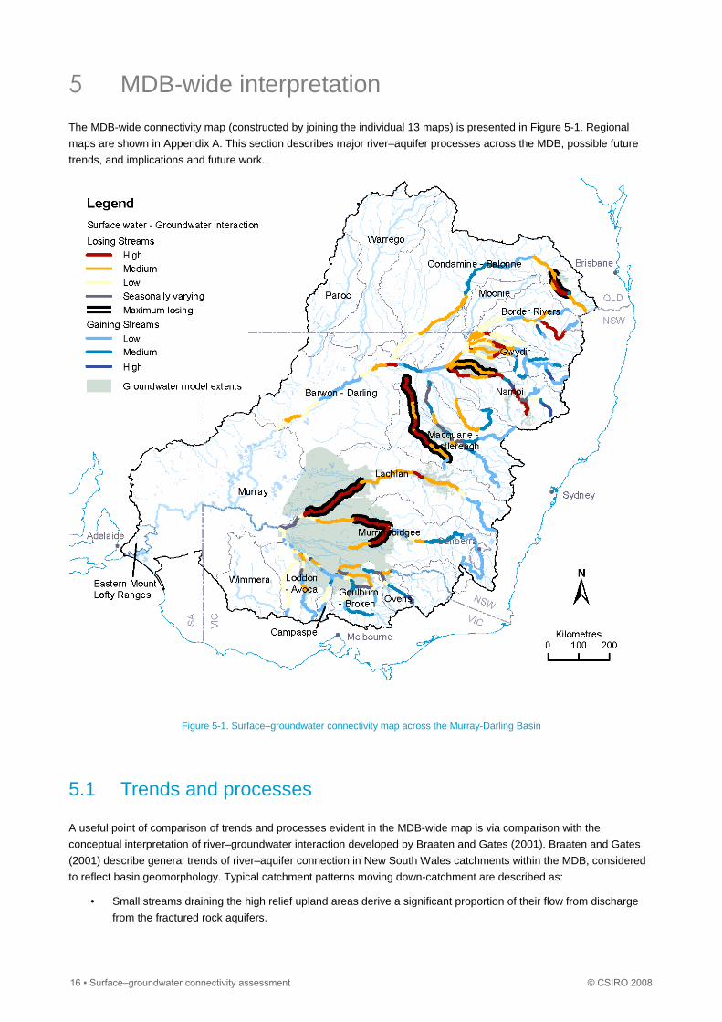
The MDB-wide connectivity map (constructed by joining the individual 13 maps) is presented in Figure 5-1. Regional
maps are shown in Appendix A. This section describes major river–aquifer processes across the MDB, possible future
trends, and implications and future work.
Figure 5-1. Surface–groundwater connectivity map across the Murray-Darling Basin
5.1 Trends and processes
A useful point of comparison of trends and processes evident in the MDB-wide map is via comparison with the
conceptual interpretation of river–groundwater interaction developed by Braaten and Gates (2001). Braaten and Gates
(2001) describe general trends of river–aquifer connection in New South Wales catchments within the MDB, considered
to reflect basin geomorphology. Typical catchment patterns moving down-catchment are described as:
• Small streams draining the high relief upland areas derive a significant proportion of their flow from discharge
from the fractured rock aquifers.
16 ▪ Surface–groundwater connectivity assessment © CSIRO 2008
• Moving from the hills into the mid-sections of the larger rivers, the alluvial systems are well developed but still
narrow and constricted by bedrock. The narrow floodplains mean that the relatively high rainfall produces
shallow alluvial watertables and strong hydraulic connection between the river and the aquifers. Flux directions
are variable along the narrow alluvial valleys and are often seasonally variable.
• As the constricted mid-sections of the rivers give way to the wider semi-arid plains of the lower valleys, water
levels begin to fall and river reaches are generally losing in nature.
• Approaching the confluence of the major inland rivers with the Darling, Barwon and Murray rivers, factors such
as basement highs and reduced aquifer transmissivity force groundwater levels near the surface again and
hence the major rivers tend to be neutral or gaining.
Generally the catchments observed follow the Braaten and Gates model quite well. In each catchment there is a distinct
change in the groundwater–river interaction as the river leaves the relatively narrow palaeovalley and enters a broad
alluvial plain to the west (or north in Victoria). This trend is evident in the Gwydir, Macquarie-Castlereagh, Lachlan,
Murrumbidgee, Ovens, Goulburn-Broken, Campaspe and Loddon-Avoca regions. The alignment of these catchments is
generally from east to west or south-east to north-west and the depth of sediments increases down the catchment as the
rivers join the Murray River. These catchments have similar geometry to the catchments described in the Braaten and
Gates model. The general pattern observed is gaining conditions in the highland areas changing to variable gaining and
losing conditions downstream within the palaeovalley, represented on the maps as ‘low losing’, ‘low gaining’ or
‘hydraulically neutral’. The flux changes to medium or high losing conditions as the river enters the large alluvial plain
before changing back towards hydraulically neutral or low gaining conditions toward the lower end of the catchment.
Differences within this general trend can be observed between the New South Wales and Victorian catchments. The
length of losing reaches in the middle to lower part of the catchment is significantly shorter in Victoria. This is in part due
to the geometry of the catchments, with the broad alluvial plains being shorter in Victoria. Further, the losing sections
within the Victorian catchments tend to be losing at a lower rate than in New South Wales. This could possibly be
influenced by the higher level of groundwater development in southern New South Wales.
Other regions within the MDB, such as the Condamine-Balonne and Namoi, do not exactly follow the Braaten and Gates
model. Within these catchments the river leaves the highland areas and the bedrock palaeovalley and enters an upper
catchment alluvial plain with an increase in sediment thickness. Downstream the rivers pass through a bedrock high
restriction, where the alluvial sediments shallow and are once again confined within a relatively narrow bedrock
palaeovalley. After passing through a bedrock choke the rivers enter a broad alluvial plain and turn towards the south-
west to eventually join the Murray River. These catchments generally behave as two Braaten and Gates model
catchments joined together, with an upper catchment and lower catchment. The upper catchment is aligned south-east to
north-west. It consists of the highland areas and an alluvial plain leading up to the bedrock choke. The lower catchment
has a north-east to south-west alignment. It begins at the bedrock choke and leads into the large alluvial plain continuing
on to the end of the catchment. The Border Rivers catchment also follows a similar trend to that of the Condamine-
Balonne and Namoi catchments; the difference is that the upper catchment alluvial plain (on the Dumaresq River and
Macintyre Brook) is much smaller than those of the Condamine-Balonne and Namoi, and hence the first Bratten and
Gates model is compressed compared to those two catchments.
Similar to the Braaten and Gates model the river fluxes observed within these catchments are roughly related to the
depth of unconsolidated sediments. Within the palaeovalley in the upper catchment the sediments are relatively shallow
with a shallow watertable and generally gaining river conditions. The depth of sediments increases on the upper alluvial
plain and consequently the groundwater levels fall relative to the river, causing generally losing conditions. Passing
through the bedrock choke areas, the depth of sediments decreases and there is a rise in the watertable causing a
reduction in river losses or change to gaining conditions. The depth of sediments increase rapidly as the rivers open out
onto the broad alluvial plain. Within these sections of the catchment the river losses are generally medium to high with
the river and groundwater often ‘disconnected’.
The connectivity mapping shows the extent and magnitude of highland gaining reaches within the Condamine-Balonne
and Border Rivers catchments are smaller than within many of the southern catchments. These findings from the
connectivity mapping fit with the findings of Neal et al. (2004). Neal et al. (2004) found significantly lower baseflow
indices (BFI) from rivers at the base of the highlands in the northern MDB catchments compared to southern catchments.
Within the northern catchments, annual baseflow indices at all gauges were classified generally between zero and 0.2. In
Victorian and southern New South Wales catchments almost all gauges recorded annual baseflow indices between 0.4
© CSIRO 2008 Surface–groundwater connectivity assessment ▪ 17

and 0.8. A similar trend can be observed in the connectivity map with a greater extent of losing conditions in the northern
part of the MDB, in the upper parts of the catchment.
Difference in climate is likely to be the main factor contributing to the change in baseflow pattern observed from the south
to the north of the MDB. In the south, rainfall is winter dominant, but in the north it is summer dominant. A higher
proportion of rainfall could therefore be ‘lost’ to evapotranspiration in the north, and hence relatively less recharge (and
hence baseflow discharge) may occur compared to the south. Other factors may also be contributing to this trend, such
as differences in rainfall intensity from north to south, topographic differences, etc. Further work would be required to
identify the key factors and their relative contribution to the observed difference in baseflow pattern.
The connectivity mapping highlighted areas where groundwater extraction is signifcantly affecting surface–groundwater
interactions. For example, the Murrumbidgee River changes from medium gaining conditions to medium losing
conditions in the vicinity of Wagga Wagga. The river changes back to gaining conditions downstream of the city. The
change to losing conditions appears to be the result of groundwater extraction rather than changing hydrogeological
conditions. In the upper Condamine-Balonne catchment, the Condamine River downstream from Warwick changes from
medium losing to ‘disconnected’ high losing conditions. The disconnected conditions at the upper end of the catchment
also appear to be the result of groundwater extraction from the alluvial aquifer. It is interesting to note in Figure 2-1 that
virtually all of the maximum losing (i.e. ‘disconnected’) reaches are coincident with areas that have been subject to
groundwater modelling (i.e. areas of the highest and most concentrated development), suggesting that ‘disconnected’
river conditions in the MDB may be largely a phenomenon occurring after groundwater development.
5.2 Future trends
Assessment of groundwater hydrographs across the MDB shows significant changes have occurred within most
catchments within the last ten years, with groundwater levels generally falling. The exceptions are the Border Rivers and
Gwydir regions where groundwater levels remained static or had risen slightly. The generally lower groundwater levels
coincide with below average rainfall over the same period. (Hydrographs from across the catchments commonly indicate
greater fluctuations in water levels within the alluvial valleys confined by bedrock rather than the broad alluvial plains.)
Response times to lower rainfall conditions are likely to be longer in mid to lower catchment areas where the river enters
the broad alluvial plains. These latter areas have deep watertables and the river and groundwater are often
‘disconnected’. These plains have significantly larger storage, and progressive fining of materials towards the end of the
catchment mean these areas normally have relatively lower hydraulic conductivities. On these broad alluvial plains with
longer response times, equilibrium conditions to the recent dry climate have probably not yet been reached. This means
river losses in hydraulically connected downstream areas of the catchments may increase in the future in response to the
dry climate over recent years. It is further anticipated that the extent of ‘disconnected’ losing streams will become more
widespread as equilibrium conditions are reached, assuming the current climate continues. Response times within the
upper catchment palaeovalleys will be more rapid than on the broad alluvial plains. These areas have relatively shallow
watertables (<10 m) and higher hydraulic conductivities (>5m /day) with a smaller storage. Due to the relatively rapid
response times within the smaller palaeovalleys the connectivity mapping is likely to approximately reflect equilibrium
conditions from the recent dry climate in these areas.
The smaller storage within the palaeovalley alluvium means that groundwater extraction has a greater impact on the
magnitude and direction of river fluxes compared to on the broad alluvial plains. In areas where the magnitude of
groundwater extraction has not changed in recent years, the palaeovalley alluvium may have reached a steady state
condition. However in areas where extraction rates have increased in recent years, the magnitude of river losses will
continue to rise in the future as the system continues to readjust.
18 ▪ Surface–groundwater connectivity assessment © CSIRO 2008

5.3 Implications and future work
SKM (2003) mapped river–aquifer interaction for major rivers across the MDB, albeit with a reduced scope compared to
that of this assessment. The SKM (2003) assessment was based on data in the late 1990s. The extent and magnitude of
losing river reaches found in this project was generally larger than that reported in SKM (2003). In particular significant
differences in river fluxes are observed on the Darling and Lachlan rivers and northern New South Wales catchments.
The differences may relate to the different dates of the two assessments, the more detailed nature of this assessment, or
a combination of these two factors.
The improved understanding of surface–groundwater interactions within the MDB provided by this assessment will have
implications for how the system is managed. There appears to be a trend of increasing extent of losing river reaches.
The extent of losing reaches may further increase in the future as the broad alluvial plain areas continue to adjust to
changed climatic conditions, time lags from groundwater development are realised, and groundwater extraction
increases in some areas. Careful management will be needed to limit exacerbation of this trend.
Identifying the extent and magnitude of river losses will enable more accurate accounting of water resources. Surface–
groundwater modelling has often previously budgeted a percentage of water as ‘unaccounted losses’. These losses may
now be accounted for as losses from the river to groundwater.
The results of the surface–groundwater connectivity mapping may also be significant for future surface water
management. On the Campaspe River, for example, losing river conditions downstream of Lake Eppalock will require
consideration when releasing flows to the river. The results may be useful in predicting the efficiency of released flows
from different locations at different times of the year.
This assessment has also highlighted the need to improve methods for identifying locations where rivers are truly
‘disconnected’ from groundwater.
It is envisaged that these connectivity maps will be updated in the future, as additional data is collected, and
improvements to the method are implemented (including those discussed in this report). In the interim however, the
maps provide a valuable tool when undertaking initial conceptualisations of surface–groundwater interactions. The maps
are an ideal tool for raising awareness of stream–aquifer interaction, and for initiating discussions regarding the process
of surface–groundwater interactions.
© CSIRO 2008 Surface–groundwater connectivity assessment ▪ 19

References
Braaten R and Gates G (2001) Groundwater – surface water interaction in inland New South Wales: a scoping study. Unpublished report, Department of Land and Water Conservation, Sydney, NSW, Australia.
Neal BP, Nathan RJ and Evans R (2004) Survey of baseflows in unregulated streams of the Murray-Darling Basin. 9th Murray-Darling Basin Groundwater Workshop, Bendigo, 17–19 February 2004.
Rassam D, Walker G and Barnett B (2008) Recommendations for modelling surface–groundwater interactions based on lessons learnt from the Murray-Darling Basin Sustainable Yields Project. A report to the Australian Government from the CSIRO Murray-Darling Basin Sustainable Yields Project. CSIRO, Australia.
SKM (2003) Projection of groundwater extraction rates and implications for future demand and competition for surface water. Murray-Darling Basin Commission, Landscapes and Industries Program. MDBC Publication 04/03.
20 ▪ Surface–groundwater connectivity assessment © CSIRO 2008
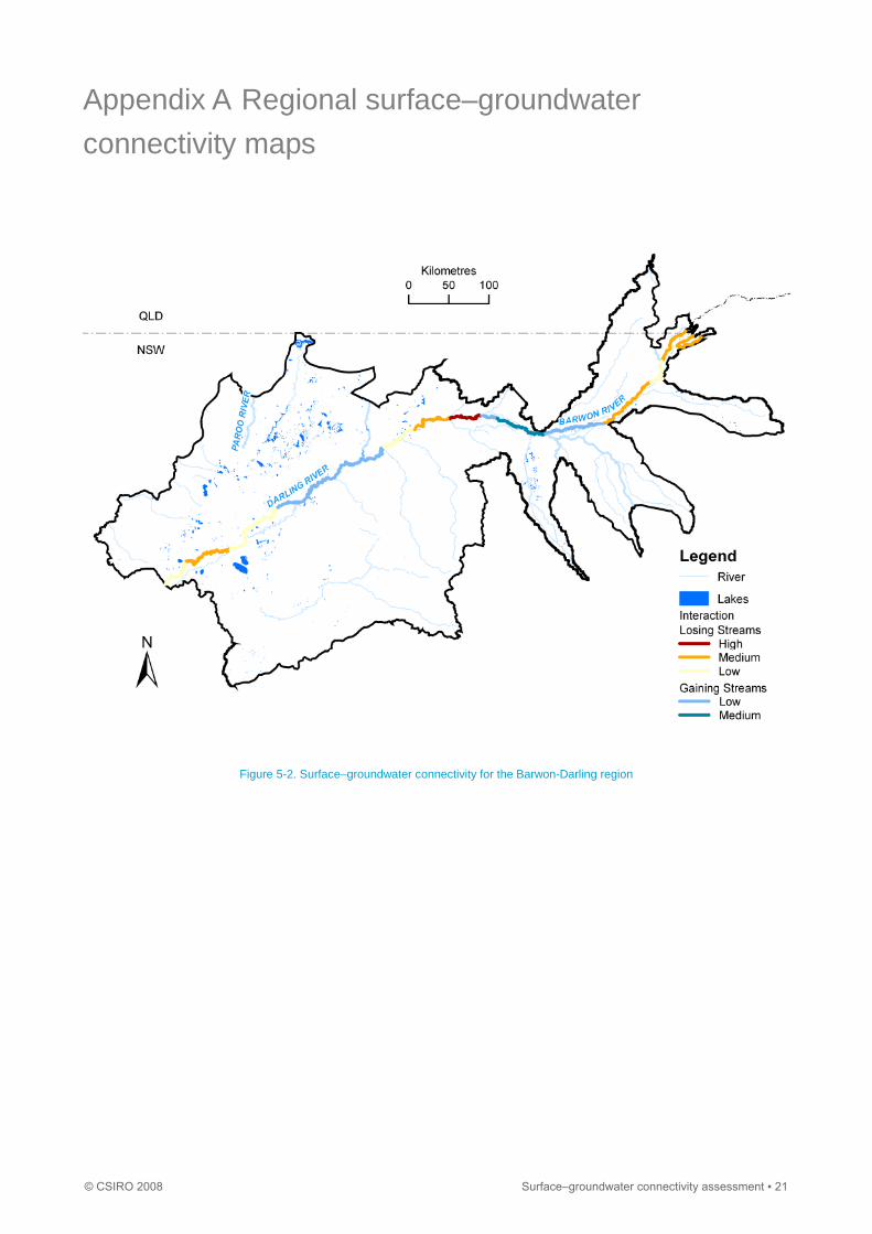
Appendix A Regional surface–groundwater
connectivity maps
Figure 5-2. Surface–groundwater connectivity for the Barwon-Darling region
© CSIRO 2008 Surface–groundwater connectivity assessment ▪ 21
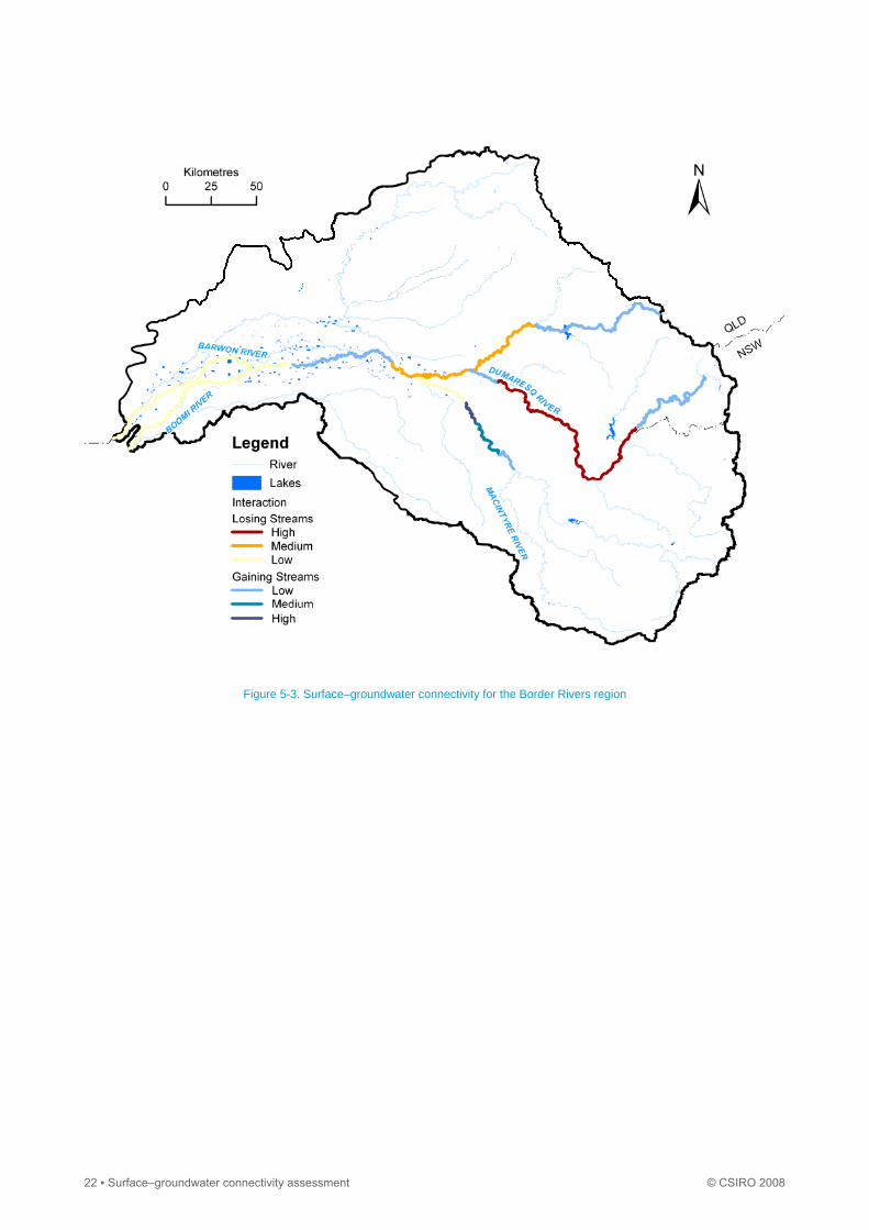
Figure 5-3. Surface–groundwater connectivity for the Border Rivers region
22 ▪ Surface–groundwater connectivity assessment © CSIRO 2008
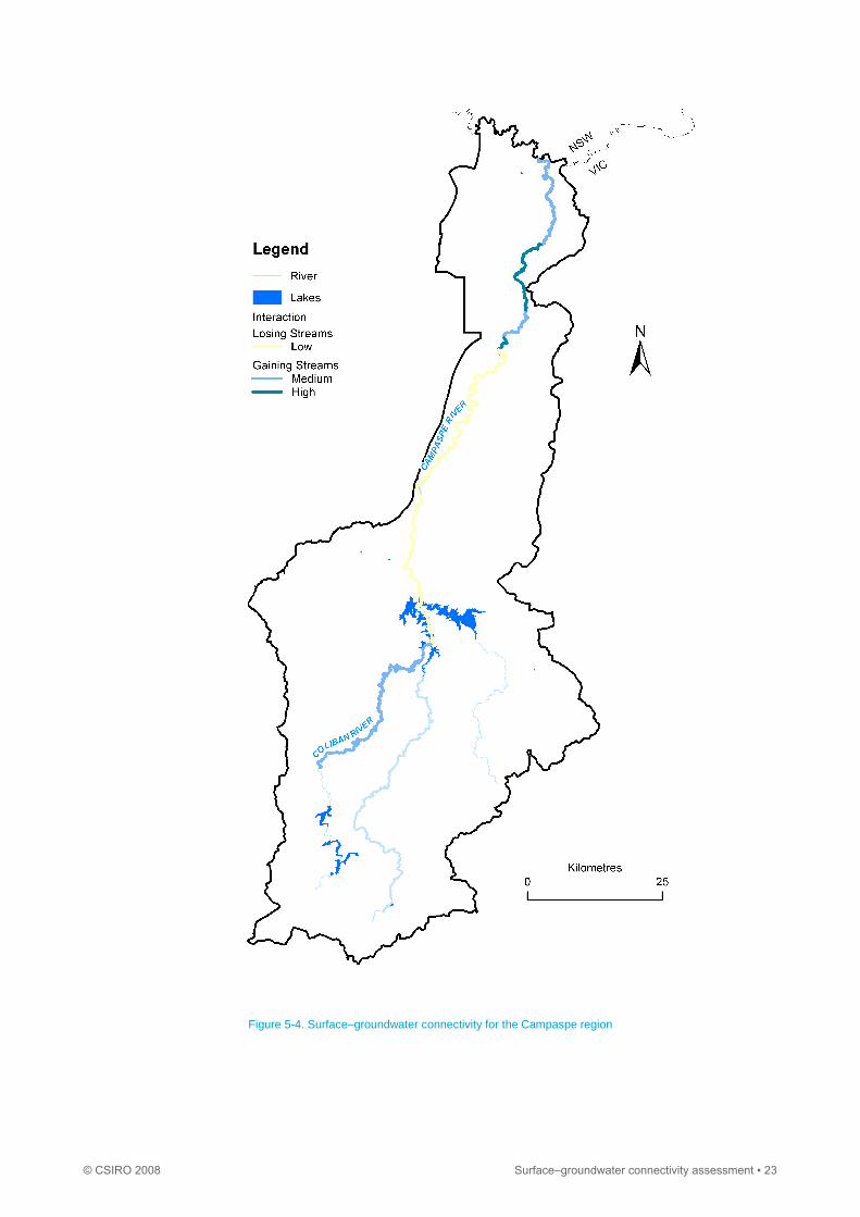
Figure 5-4. Surface–groundwater connectivity for the Campaspe region
© CSIRO 2008 Surface–groundwater connectivity assessment ▪ 23
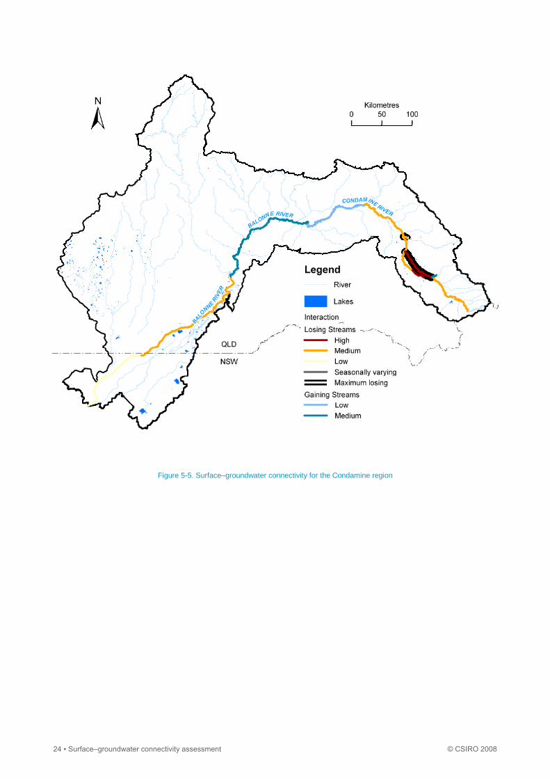
Figure 5-5. Surface–groundwater connectivity for the Condamine region
24 ▪ Surface–groundwater connectivity assessment © CSIRO 2008
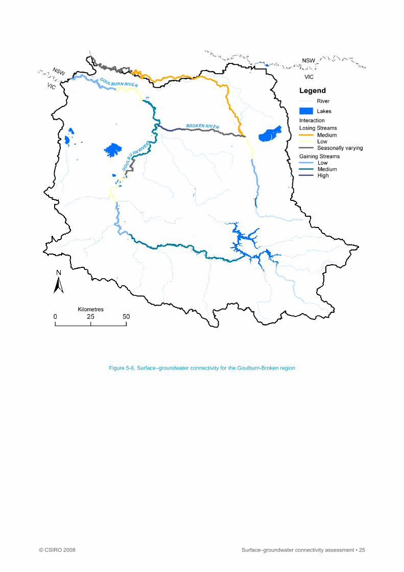
Figure 5-6. Surface–groundwater connectivity for the Goulburn-Broken region
© CSIRO 2008 Surface–groundwater connectivity assessment ▪ 25
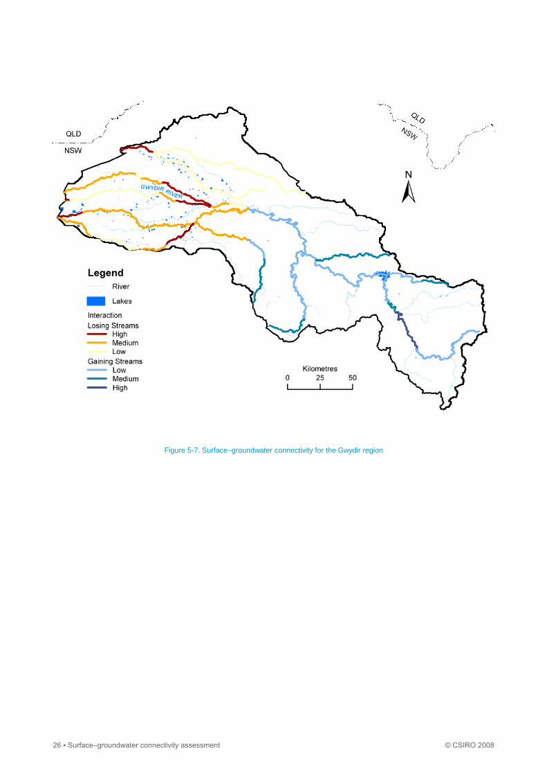
Figure 5-7. Surface–groundwater connectivity for the Gwydir region
26 ▪ Surface–groundwater connectivity assessment © CSIRO 2008

Figure 5-8. Surface–groundwater connectivity for the Lachlan region
© CSIRO 2008 Surface–groundwater connectivity assessment ▪ 27
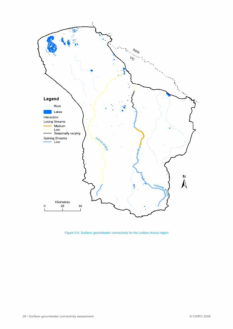
Figure 5-9. Surface–groundwater connectivity for the Loddon-Avoca region
28 ▪ Surface–groundwater connectivity assessment © CSIRO 2008
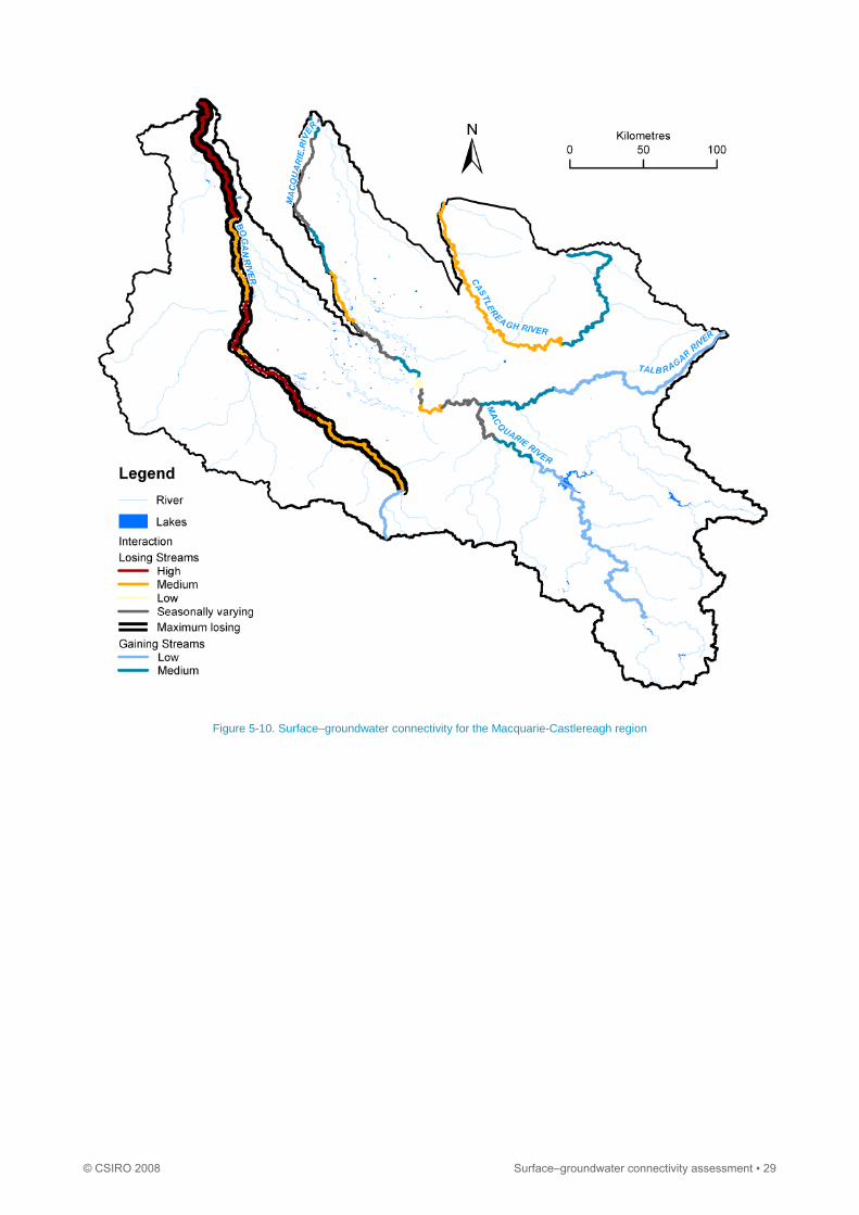
Figure 5-10. Surface–groundwater connectivity for the Macquarie-Castlereagh region
© CSIRO 2008 Surface–groundwater connectivity assessment ▪ 29
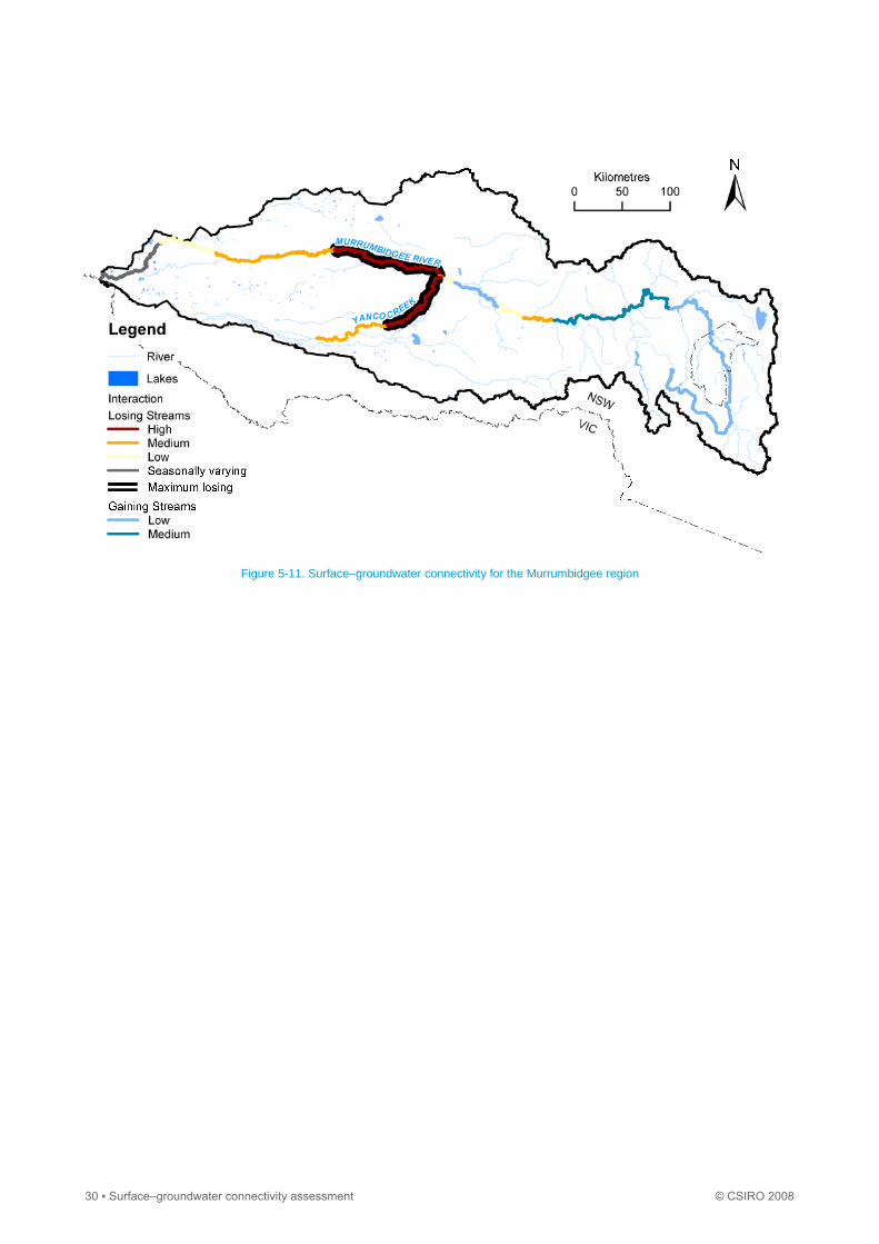
Figure 5-11. Surface–groundwater connectivity for the Murrumbidgee region
30 ▪ Surface–groundwater connectivity assessment © CSIRO 2008

Figure 5-12. Surface–groundwater connectivity for the Murray region
© CSIRO 2008 Surface–groundwater connectivity assessment ▪ 31

Figure 5-13. Surface–groundwater connectivity for the Namoi region
32 ▪ Surface–groundwater connectivity assessment © CSIRO 2008
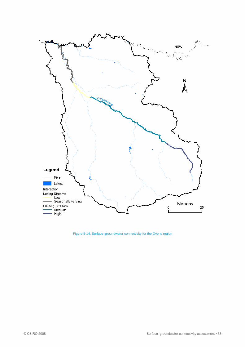
Figure 5-14. Surface–groundwater connectivity for the Ovens region
© CSIRO 2008 Surface–groundwater connectivity assessment ▪ 33

Recommended