Supporting Information for A Magnon Scattering Platform Tony X. Zhou*, Joris J. Carmiggelt, Lisa M. Gächter, Ilya Esterlis, Dries Sels, Rainer J. Stöhr,

Chunhui Du, Daniel Fernandez, Joaquin F. Rodriguez-Nieva, Felix Büttner, Eugene Demler and

Amir Yacoby*

*correspondence to: gztony1227@gmail.com and yacoby@physics.harvard.edu

Contents A Magnon Scattering Platform ....................................................................................................... 1

Section S1: Sample fabrication ....................................................................................................... 3

Section S2: Experimental setup and inference scheme to determine phase of magnons ................ 3

Section S3: Modeling the magnon modes excited by the stripline ................................................. 3

Section S4: Magnon dispersion and additional notes for characterizing the generation of magnons from the stripline ............................................................................................................. 4

Section S5: Calculation of the total AC magnetic field the NV center .......................................... 5

Section S6. Rabi oscillation measurements .................................................................................... 7

Section S7. Derivation of Green’s function associated to magnons in YIG ................................... 8

Section S8. Details of scattering model ........................................................................................ 11

Section S9. Feasibility to study 2D magnetic materials ............................................................... 13

Section S10. Importance of low damping material as “vacuum” ................................................. 14

Section S11. Variation in Figure 2 line cut data ........................................................................... 15

Section S12. Supporting Movie (.mp4) ........................................................................................ 16

Section S1: Sample fabrication The 100 nm thick YIG film was grown on a GGG substrate and purchased commercially from Matesy GmbH. We used photolithography to pattern the stripline onto the YIG film. We deposit 100 nm gold (Au) and a 10 nm titanium (Ti) adhesion layer by e-beam evaporation. The sample went through a second lithography step to define the Permalloy (Py) target. Py disks 100nm thick were deposited via thermal evaporation. Before each metal deposition step, we used O2 plasma cleaning to remove any resist residue. The resulting Au stripline is 10 µm wide, and the Py disk has a diameter of 5 µm and is 110 um away from the stripline. An optical micrograph of this device can be seen in Fig S1. Additional alignment marks shown as half circles located on the lower right corner of Fig 4 are used to provide drift corrections.

Section S2: Experimental setup and inference scheme to determine phase of magnons

All measurements were performed at room temperature using a home-built optical confocal setup1. A single NV center is embedded in the nanopillar that sits at the very end of the diamond probe2,3, which is read out optically. To use scanning NV center magnetometer (Fig. S2) for imaging magnons, the NV center was selected such that its orientation in the diamond lattice is parallel to the stripline on the YIG to guarantee excitation of magnons in the Damon-Eshbach geometry. The microwave currents used to excite magnons were generated by an amplified Rhode-Schwarz SMB100A microwave source. The reference field required to measure the magnonic phase was applied by a distant micro-positioned current loop (antenna) connected to a second Rhode-Schwarz microwave source. The relative phase Δ𝜙𝜙 between the two RF sources is locked and controlled by software. Δ𝜙𝜙 here is the 𝜙𝜙 in main text which corresponds to setting the phase of the reference field to zero.

Section S3: Modeling the magnon modes excited by the stripline

We excite magnons in a 100 nm thin YIG film by sending a RF current through the stripline. Defining the y direction along the microstrip and the z direction normal to the YIG plane, the excited magnons will propagate in the x direction, due to the symmetry of the wire. All our experiments are performed in the Damon-Eshbach geometry, which demands that the external magnetic field points in the y-direction4. Note that with the YIG magnetized in the y-direction, only the x and z components of the driving field can apply a torque on the spins and induce magnons in the YIG (the y-component of the field generated by the microstrip is zero). By solving the Landau-Lifthitz-Gilbert equation in a thins slab, it can be shown that the x component will induce magnons most efficiently due to the demagnetizing field5.

Magnon modes with a certain k vector are efficiently excited by the stripline when the Fourier transform of the spatial profile of the driving field has a large amplitude at that particular

wavevector6,7. We simulated the spatial field profile using a micromagnetic finite-element solver (CST microwave studio, Student edition). This program numerically calculates the stray field of the microstrip, taking into account all kinds of dielectric effects such as the skin effect. The field profile together with its Fourier transform are depicted in Fig. S3, which allows us to predict the magnon spectrum that is excited in the YIG.

Section S4: Magnon dispersion and additional notes for characterizing the generation of magnons from the stripline In this section, we describe how the magnetic stray field of magnons in Damon-Eshbach geometry directly drive the NV spin. Andrich et al.8 and Kikuchi et al.9 show a proof of this concept by measuring magnon driven Rabi oscillations and ESR contrast from NVs embedded in nanodiamonds that are located directly on top of the YIG. We used a single NV center in a scanning probe to analyze the excited magnon spectrum. Note that the NV can only probe magnons with frequencies equal to its ESR frequency. The frequency of a Damon-Eshbach magnon depends on the magnitude of the external magnetic field and its wavevector k via its dispersion4:

𝑓𝑓DESW = 𝛾𝛾�(𝐵𝐵extsin(𝜃𝜃ext − Δ𝜃𝜃) +𝑀𝑀𝑠𝑠

2)2 − �

𝑀𝑀𝑠𝑠

2�2

exp( − 2𝑘𝑘𝑘𝑘) (S1)

In this formula 𝑓𝑓DESW is the frequency of the magnons in GHz which is the same as that of the RF driving field used to excite the magnon, 𝐵𝐵ext is the external magnetic field component parallel to the NV axis, 𝑀𝑀𝑠𝑠 is the saturation magnetization, γ is the electronic gyromagnetic ratio, l is the thickness of the YIG film and k is the wavenumber of the excited magnon mode. Since the NV-axis is oriented at 𝜃𝜃ext = 54.74° with respect to the surface normal, a sine is added to calculate the magnetic field component parallel to the YIG spins. Although the YIG spins are kept largely in the plane by the demagnetizing field, a slight canting of the spins out of the plane will occur due to the externally applied magnetic field. The canting angle Δ𝜃𝜃 can be calculated by numerically solving the following equation10:

𝜇𝜇0𝑀𝑀𝑠𝑠sin(2(90° − |Δ𝜃𝜃|)) − 2𝐵𝐵extsin(90° − |Δ𝜃𝜃| − 𝜃𝜃ext) = 0 (S2) Here 𝜇𝜇0 is the vacuum permeability. Fig. S4 shows the angles for the magnetic fields considered in this work, showing a maximal canting angle of approximately 5°. The magnon dispersion in equation S1 is in principle only valid for in-plane magnetizations and can be generalized for magnetizations with an out-of-plane component via the formulas in reference11. We also performed our analysis using these formulas but did not observe any notable differences compared to the analysis using equation S1, presumably due to the relatively small external magnetic fields we consider in this work. An important note is that the external magnetic field 𝐵𝐵ext is used to simultaneously tune the excitation of magnons in YIG and the Zeeman splitting of the NV’s spin states: by changing 𝐵𝐵ext both the ESR frequency and the k-vector of the excited magnons are changed at the same time, assuming the RF frequency of the driving field is kept constant. This concept is illustrated in Fig.

1b, and Fig. S5, which is a three-dimensional attempt to show that for different ESR frequencies we probe magnons with different k values. The shading illustrates the excitation efficiency of these magnons that fluctuate proportional to the Fourier amplitude of the excitation field as was described in the previous section. Using equations S1 and S2, we calculated the frequencies of the wavevectors that are excited the least efficiently by the stripline (corresponding to the FFT minima in Fig. S2) at different external magnetic fields 𝐵𝐵ext. We optimized 𝑀𝑀𝑠𝑠, 𝑘𝑘 and 𝜃𝜃ext such that the calculated frequencies of the minima matched the observed minima in ESR and Rabi frequencies depicted in Fig. 3d the best. The arrows indicated in Fig. 3d and dashed lines in Fig. 3c correspond to the frequency of the minima for 𝑀𝑀𝑠𝑠 = 1740 G, 𝑘𝑘 = 97 nm and 𝜃𝜃ext = 54.74°. Note that for these parameters also the observed ferromagnetic resonance (FMR) in Fig. 3c is reasonably matched to its analytical linetrace. For Fig. 3b we inverted equation S1 in order to convert the ESR frequencies to wavevectors and again optimized parameters to match the ESR and FFT minima. We find 𝑀𝑀𝑠𝑠 =1740 G, 𝑘𝑘 = 97 nm and 𝜃𝜃ext = 50.74°. Since the data in Fig. 3b was taken with a different probe than the data in Fig. 3c and 3d, we attribute the small deviation in 𝜃𝜃ext to slight tip-mounting differences between probes.

Section S5: Calculation of the total AC magnetic field the NV center In our experiments (Fig. 2, a, b, and c), we rely on the driving of the NV spin via the microwave fields generated by magnons. In this section, we analytically calculate the spatial profile of the magnon microwave field, which is used to fit the data presented in the main text. Due to the demagnetizing field of the YIG film, the magnetization precession of magnons is slightly elliptical, having the largest perturbation in magnetization in the 𝑥𝑥lab direction (measured in the lab frame). Therefore, the magnon’s magnetization is described by:

𝑀𝑀𝑥𝑥lab = 𝑀𝑀𝑒𝑒𝑖𝑖(𝑘𝑘𝑥𝑥lab−𝜔𝜔𝜔𝜔) 𝑀𝑀𝑧𝑧lab = −𝑖𝑖𝑀𝑀𝜂𝜂𝑒𝑒𝑖𝑖(𝑘𝑘𝑥𝑥lab−𝜔𝜔𝜔𝜔)

(S9)

Here, 𝑘𝑘 and 𝜔𝜔 are the wavevector and angular frequency of the magnons, 𝑀𝑀 corresponds to the transverse component of the magnetization in the 𝑥𝑥lab direction and 𝜂𝜂 < 1 indicates the ellipticity of the magnons. Using references12,13, we can calculate the magnetic field components generated by this magnetization texture at a distance d from the YIG surface. Surprisingly, we find that the magnons generate circular magnetic fields, independent of the magnon ellipticity 𝜂𝜂:

𝐵𝐵𝑥𝑥labSW(𝑘𝑘,𝑑𝑑) = −

𝜇𝜇0𝑀𝑀2

(1 + 𝜂𝜂)𝑘𝑘𝑒𝑒−𝑘𝑘𝑘𝑘𝑒𝑒𝑖𝑖(𝑘𝑘𝑥𝑥lab−𝜔𝜔𝜔𝜔)

= −𝜇𝜇0𝑀𝑀

2(1 + 𝜂𝜂)𝑘𝑘𝑒𝑒−𝑘𝑘𝑘𝑘cos(𝑘𝑘𝑥𝑥lab − 𝜔𝜔𝜔𝜔)

(S10)

𝐵𝐵𝑧𝑧labSW(𝑘𝑘,𝑑𝑑) = −𝑖𝑖

𝜇𝜇0𝑀𝑀2

(1 + 𝜂𝜂)𝑘𝑘𝑒𝑒−𝑘𝑘𝑘𝑘𝑒𝑒𝑖𝑖(𝑘𝑘𝑥𝑥lab−𝜔𝜔𝜔𝜔)

=𝜇𝜇0𝑀𝑀

2(1 + 𝜂𝜂)𝑘𝑘𝑒𝑒−𝑘𝑘𝑘𝑘sin(𝑘𝑘𝑥𝑥lab − 𝜔𝜔𝜔𝜔)

Here, 𝜇𝜇0 is the vacuum permeability, SW denotes for spin wave (magnon), and we took the real part of field in the last step. 𝐵𝐵𝑦𝑦lab

(𝑘𝑘,𝑑𝑑) = 0 due to the symmetry of the system. To estimate how efficient the NV spin is driven by the magnon field, we calculate the component of the field perpendicular to the NV axis, since only this component drives the NV spin. We thus transform the fields to the NV’s reference frame (in which the z-axis overlaps with the NV axis) via the following basis transformation.

𝑥𝑥 = 𝑥𝑥lab

𝑦𝑦 = −𝑧𝑧labsin(54.74°) + 𝑦𝑦labcos(54.74°)

𝑧𝑧 = 𝑧𝑧labcos(54.74°) + 𝑦𝑦labsin(54.74°)

(S11)

Note that an elliptical projection of the magnon field in the xy-plane is driving the NV spin. Finally, we assume that the reference field 𝐵𝐵Ref is linear and that it drives the NV at an arbitrary angle 𝜙𝜙sp in the xy-plane at a frequency 𝜔𝜔Ref, such that:

𝐵𝐵𝑥𝑥Ref = 𝐴𝐴cos𝜙𝜙spcos(𝜔𝜔Ref𝜔𝜔)

𝐵𝐵𝑦𝑦Ref = 𝐴𝐴sin𝜙𝜙spcos(𝜔𝜔Ref𝜔𝜔) (S12)

By performing the basis transformation described in equation S11 and writing 𝐵𝐵 =𝜇𝜇0𝑀𝑀2

(1 + 𝜂𝜂)𝑘𝑘𝑒𝑒−𝑘𝑘𝑘𝑘, we can now construct the Hamiltonian of our system:

𝐻𝐻 = 𝐵𝐵NV𝜎𝜎𝑧𝑧 + �𝐴𝐴cos𝜙𝜙spcos(𝜔𝜔Ref𝜔𝜔) − 𝐵𝐵cos(𝑘𝑘𝑥𝑥 + 𝜔𝜔SW𝜔𝜔 + Δ𝜙𝜙)�𝜎𝜎𝑥𝑥 (𝐴𝐴sin𝜙𝜙spcos(𝜔𝜔Ref𝜔𝜔) − 𝐵𝐵sin(𝑘𝑘𝑥𝑥 + 𝜔𝜔SW𝜔𝜔 + Δ𝜙𝜙)sin(54.74°))𝜎𝜎𝑦𝑦

(S13)

Here, 𝐵𝐵ext is the stationary magnetic field applied along the NV axis that is used to Zeeman split the NV spin levels, 𝜎𝜎𝑥𝑥 and 𝜎𝜎𝑦𝑦 are the Pauli spin matrices. Furthermore, we allowed the reference field and the magnon field to have a relative phase difference Δ𝜙𝜙. Note: Δ𝜙𝜙 here is the 𝜙𝜙 in main text by setting phase of reference field to be zero for math symbol simplification. In our experiments the frequency of both sources are tuned to the spin transition frequency ω of the NV, such that 𝜔𝜔SW = 𝜔𝜔Ref = 𝜔𝜔. Next, we rewrite the Hamiltonian in the frame rotating at frequency ω:

𝐻𝐻 = �𝐴𝐴cos𝜙𝜙spcos𝜔𝜔𝜔𝜔 − 𝐵𝐵cos(𝑘𝑘𝑥𝑥 + 𝜔𝜔𝜔𝜔 + Δ𝜙𝜙)� �cos𝜔𝜔𝜔𝜔 ∙ 𝜎𝜎𝑥𝑥 + sin𝜔𝜔𝜔𝜔 ∙ 𝜎𝜎𝑦𝑦�+ �𝐴𝐴sin𝜙𝜙spcos𝜔𝜔𝜔𝜔 + 𝐵𝐵sin(𝑘𝑘𝑥𝑥 + 𝜔𝜔𝜔𝜔 + Δ𝜙𝜙)sin(54.74°)��-sin𝜔𝜔𝜔𝜔 ∙ 𝜎𝜎𝑥𝑥+ cos𝜔𝜔𝜔𝜔 ∙ 𝜎𝜎𝑦𝑦�

(S14)

By using the product-sum trigonometric identities and after applying the Rotating Wave Approximation, we finally find:

𝐻𝐻 = �𝐴𝐴 cos𝜙𝜙sp + 𝐵𝐵 cos(𝑘𝑘𝑥𝑥 + Δ𝜙𝜙)(−1 + sin(54.74°)�𝜎𝜎𝑥𝑥+ �𝐴𝐴 sin𝜙𝜙sp − 𝐵𝐵sin(𝑘𝑘𝑥𝑥 + Δ𝜙𝜙)(−1 + sin(54.74°)�𝜎𝜎𝑦𝑦= 𝛼𝛼𝜎𝜎𝑥𝑥 + 𝛽𝛽𝜎𝜎𝑦𝑦

(S15)

We can now calculate the magnitude of the RF field perpendicular to the NV plane:

|𝐵𝐵RF| = �𝛼𝛼2 + 𝛽𝛽2 (S16)

= �𝐴𝐴2 + 𝐵𝐵2(−1 + sin(54.74°)2 + 2𝐴𝐴𝐵𝐵(1 + sin(54.74°)( cos𝜙𝜙spcos(𝑘𝑘𝑥𝑥 + Δ𝜙𝜙) + sin𝜙𝜙spsin(𝑘𝑘𝑥𝑥 + Δ𝜙𝜙))

It is now clear that changing the relative phase difference between the sources Δ𝜙𝜙 effectively corresponds to moving in x. The equation is symmetric under exchange of 𝜙𝜙sp and 𝑘𝑘𝑥𝑥 + Δ𝜙𝜙, which shows that changing x also corresponds to changing 𝜙𝜙sp. In the end we are interested in |𝐵𝐵RF| at different NV positions x for a static value of 𝜙𝜙sp and Δ𝜙𝜙. Since these parameters only shift the function in x, we can just as well evaluate |𝐵𝐵RF| for 𝜙𝜙sp = Δ𝜙𝜙 = 0. This simplifies the equation to:

|𝐵𝐵RF| = �(𝐴𝐴2 + 𝐵𝐵2(−1 + sin(54.74°))2 + 2𝐴𝐴𝐵𝐵(−1 + sin(54.74°))cos𝑘𝑘𝑥𝑥 (S17) It is now evident that the largest interference field is obtained at 𝑘𝑘𝑥𝑥 = 𝑛𝑛 ∙ 2𝜋𝜋, whereas the field is minimized at 𝑘𝑘𝑥𝑥 = 𝑛𝑛 ∙ 𝜋𝜋 (with n, an integer). By changing x, one effectively changes the phase difference between the two fields, which rotates the stationary magnon field with respect to the reference field in the plane perpendicular to the NV axis. It is clear that the contrast between both x values is maximal if 𝐴𝐴 = 𝐵𝐵�−1 + sin(54.74°)� = 𝐵𝐵total. Therefore, we calibrate the RF powers of the magnons and reference field to be approximately equal prior to each imaging measurements. This leaves us with a final expression for |𝐵𝐵RF| at the position of the NV center:

|𝐵𝐵RF| = √2𝐵𝐵Rabi�1 + cos(𝑘𝑘𝑥𝑥) (S18) The detected NV photoluminescence should be proportional to |𝐵𝐵RF|. We thus used equation S17 to fit the data of Fig. 2c in the main text, which fits the data very well.

Section S6. Rabi oscillation measurements

The NV center is a spin qubit that consists of a two-level system. A coherent AC magnetic field can drive the population of NV center between its ground state 𝑚𝑚𝑠𝑠 = 0 and excited state 𝑚𝑚𝑠𝑠 = −1 via Rabi oscillation. The measurement sequence and typical data and analysis are shown

in (Fig. S2). In most of our experiments, the AC magnetic field is generated by coherent magnons. The magnon population density is therefore proportional to the amplitude of the AC magnetic field applied at the NV electron spin resonance (ESR) frequency. This amplitude can be precisely quantified by measuring the NV spin rotation rate (Rabi frequency) 𝑓𝑓R. The Rabi frequency is given by 𝑓𝑓R = 𝛾𝛾𝐵𝐵AC⊥

2𝜋𝜋√2, where 𝐵𝐵AC⊥ is the component of the drive field perpendicular to the NV axis,

and γ2𝜋𝜋

= 28 GHz/T is the electron spin gyromagnetic ratio.

Section S7. Derivation of Green’s function associated to magnons in YIG

In this section we summarize the model of magnetostatic waves in a tangentially magnetized thin film and present analysis of scattering of Damon-Eshbach surface waves by the Py disc (Fig. S7).

Theoretical analysis begins by decomposing the magnetic field 𝐇𝐇 and magnetization 𝐌𝐌 into static and fluctuating components:

𝐇𝐇 = 𝐻𝐻0𝐲𝐲� + 𝐡𝐡𝑒𝑒−𝑖𝑖𝜔𝜔𝜔𝜔, 𝐌𝐌 = 𝑀𝑀𝑆𝑆𝐲𝐲� + 𝐦𝐦𝑒𝑒−𝑖𝑖𝜔𝜔𝜔𝜔. (S19) Here 𝐻𝐻0 is the magnitude of the static bias field that polarizes the magnet and we take it to lie along 𝐲𝐲�. Quantity 𝑀𝑀𝑆𝑆 is the saturated magnetization of the magnitude. The geometry is shown in Fig. S7. In the absence of impurities, the fluctuations satisfy the following form of the “magnetostatic” Maxwell equations4:

∇ × 𝐡𝐡 = 0, ∇ ⋅ (𝐡𝐡 + 4𝜋𝜋𝐦𝐦) = 0. (S20) These equations are valid in the regime where the wavelength of light in the medium is much shorter than the free space wavelength. For the frequency range under consideration, the free space wavelength is on the order of centimeters while the wavelength of magnetostatic waves is on the order of microns. The magnetostatic approximation therefore holds to a good approximation in the present context.

The dynamics of 𝑀𝑀 is related to 𝐻𝐻 via the Landau-Lifshitz equation14 𝑘𝑘𝑀𝑀

𝑘𝑘𝜔𝜔= −𝛾𝛾𝑀𝑀 × 𝐻𝐻, (S21)

where 𝛾𝛾 is the electron gyromagnetic ratio. Expanding this for small fluctuations using (S19), the small-signal magnetization 𝐦𝐦 is related to 𝐡𝐡 according to

4𝜋𝜋𝐦𝐦 = �̂�𝜒(𝜔𝜔) ⋅ 𝐡𝐡, (S22) where �̂�𝜒(𝜔𝜔) is the “Polder susceptibility tensor” and has the explicit form4

�̂�𝜒 = �𝜒𝜒 0 𝑖𝑖𝜅𝜅0 0 0−𝑖𝑖𝜅𝜅 0 𝜒𝜒

�, (S23)

where 𝜒𝜒 = 𝜔𝜔0𝜔𝜔𝑀𝑀

𝜔𝜔02−𝜔𝜔2 , 𝜅𝜅 = 𝜔𝜔𝜔𝜔𝑀𝑀

𝜔𝜔02−𝜔𝜔2, (S24)

and 𝜔𝜔0 = 𝛾𝛾𝐻𝐻0, 𝜔𝜔𝑀𝑀 = 4𝜋𝜋𝛾𝛾𝑀𝑀𝑆𝑆. We note this form of the susceptibility tensor ignores exchange coupling in the magnet. In YIG these exchange effects only become operational for wavelengths on the order of a fraction of micron. Given the wavelengths under consideration on the order of tens of microns, exchange coupling can therefore be safely neglected.

The first magnetostatic equation implies we may write 𝐡𝐡 = −∇𝜓𝜓. The second magnetostatic equation then becomes

𝜕𝜕2𝜓𝜓𝜕𝜕𝑦𝑦2

+ (1 + 𝜒𝜒) �𝜕𝜕2𝜓𝜓𝜕𝜕𝑥𝑥2

+ 𝜕𝜕2𝜓𝜓𝜕𝜕𝑧𝑧2

� = 0 (|𝑧𝑧| < 𝑑𝑑/2), (S25)

𝜕𝜕2𝜓𝜓𝜕𝜕𝑥𝑥2

+ 𝜕𝜕2𝜓𝜓𝜕𝜕𝑦𝑦2

+ 𝜕𝜕2𝜓𝜓𝜕𝜕𝑧𝑧2

= 0. (|𝑧𝑧| > 𝑑𝑑/2). (S26) The freely propagating modes in the magnet are then obtained by solving these equations, subject to the usual boundary conditions of continuity of the tangential components of 𝐡𝐡 and continuity of the normal component of 𝐡𝐡 + 4𝜋𝜋𝐦𝐦.

We incorporate the magnetic target by addition of an AC source 𝐦𝐦imp to the magnetization 𝐦𝐦, localized just about the surface of the magnet. This modifies the equation for 𝜓𝜓 according to

𝜕𝜕2𝜓𝜓𝜕𝜕𝑥𝑥2

+ 𝜕𝜕2𝜓𝜓𝜕𝜕𝑦𝑦2

+ 𝜕𝜕2𝜓𝜓𝜕𝜕𝑧𝑧2

= 4𝜋𝜋∇ ⋅ 𝐦𝐦imp (𝑧𝑧 > 𝑑𝑑/2), (S27) We remark that this ignores DC coupling between the target and the underlying YIG, that is, we neglect modifications of the local permeability seen by the magnons due to the static magnetization of the target.

The general response of the system can be expressed in terms of the Green’s function 𝐺𝐺(𝐫𝐫 − 𝐫𝐫0), which describes waves created by a point source at position 𝐫𝐫0 in the region 𝑧𝑧 > 𝑑𝑑/2. Thus we need to solve the wave equation

𝜕𝜕2𝐺𝐺𝜕𝜕𝑥𝑥2

+ 𝜕𝜕2𝐺𝐺𝜕𝜕𝑦𝑦2

+ 𝜕𝜕2𝐺𝐺𝜕𝜕𝑧𝑧2

= 0 (𝑧𝑧 < −𝑑𝑑/2), (S28)

𝜕𝜕2𝐺𝐺𝜕𝜕𝑦𝑦2

+ (1 + 𝜒𝜒) �𝜕𝜕2𝐺𝐺𝜕𝜕𝑥𝑥2

+ 𝜕𝜕2𝐺𝐺𝜕𝜕𝑧𝑧2

� = 0 (|𝑧𝑧| < 𝑑𝑑/2), (S29)

𝜕𝜕2𝐺𝐺𝜕𝜕𝑥𝑥2

+ 𝜕𝜕2𝐺𝐺𝜕𝜕𝑦𝑦2

+ 𝜕𝜕2𝐺𝐺𝜕𝜕𝑧𝑧2

= 𝛿𝛿(𝐫𝐫 − 𝐫𝐫0) (𝑧𝑧 > 𝑑𝑑/2). (S30) with 𝑧𝑧0 > 𝑑𝑑/2. To find 𝐺𝐺 we first make the 2D Fourier transform of (𝑥𝑥,𝑦𝑦) coordinates

𝐺𝐺(𝝆𝝆 − 𝝆𝝆0, 𝑧𝑧 − 𝑧𝑧0) = ∫ 𝑘𝑘2𝐤𝐤2𝜋𝜋

𝑒𝑒𝑖𝑖𝐤𝐤⋅(𝝆𝝆−𝝆𝝆0)𝐺𝐺�(𝐤𝐤, 𝑧𝑧 − 𝑧𝑧0), (S31) where we define the 2D vector 𝝆𝝆 = 𝑥𝑥𝐱𝐱� + 𝑦𝑦𝐲𝐲�. The wave equation then simplifies to an ordinary differential equation in 𝑧𝑧:

𝐺𝐺′� ′ − 𝑘𝑘2𝐺𝐺� = 0 (𝑧𝑧 < −𝑑𝑑/2), (S32) (1 + 𝜒𝜒)𝐺𝐺′� ′ − (𝑘𝑘2 + 𝜒𝜒𝑘𝑘𝑥𝑥2)𝐺𝐺� = 0 (|𝑧𝑧| < 𝑑𝑑/2), (S33) 𝐺𝐺′� ′ − 𝑘𝑘2𝐺𝐺� = 𝛿𝛿(𝑧𝑧 − 𝑧𝑧0) (𝑧𝑧 > 𝑑𝑑/2). (S34)

where primes denote derivatives with respect to 𝑧𝑧. The solutions in the different regions are 𝐺𝐺�(𝐤𝐤, 𝑧𝑧) = 𝐺𝐺�𝐼𝐼,0𝑒𝑒𝑘𝑘𝑧𝑧 (𝑧𝑧 < −𝑑𝑑/2), (S35) 𝐺𝐺�(𝐤𝐤, 𝑧𝑧) = 𝐺𝐺�𝐼𝐼𝐼𝐼,0+ 𝑒𝑒𝑘𝑘�𝑧𝑧 + 𝐺𝐺�𝐼𝐼𝐼𝐼,0− 𝑒𝑒−𝑘𝑘�𝑧𝑧 (|𝑧𝑧| < 𝑑𝑑/2), (S36) 𝐺𝐺�(𝐤𝐤, 𝑧𝑧) = − 1

2𝑘𝑘𝑒𝑒−𝑘𝑘|𝑧𝑧−𝑧𝑧0| + 𝐺𝐺�𝐼𝐼𝐼𝐼𝐼𝐼,0𝑒𝑒−𝑘𝑘𝑧𝑧 (𝑧𝑧 > 𝑑𝑑/2). (S37)

where quantities with “0” subscripts denote coefficients of homogeneous solutions and we define 𝑘𝑘�2 = 𝑘𝑘2+𝜒𝜒𝑘𝑘𝑥𝑥2

1+𝜒𝜒. (S38)

The solutions above have been chosen such that 𝐺𝐺� vanishes as |𝑧𝑧| → ∞. The function 𝐺𝐺�(𝐤𝐤, 𝑧𝑧) is then uniquely determined by applying the various boundary conditions across the surface of the magnet. The complete solution is rather cumbersome so here we report the result in the limit 𝑧𝑧0 →𝑑𝑑/2; i.e., the limit in which the impurity approaches the surface of the magnet:

𝐺𝐺�(𝐤𝐤, 𝑧𝑧) = 𝑒𝑒−𝑘𝑘(𝑧𝑧−𝑑𝑑/2)

𝑘𝑘

× 1+𝜅𝜅cos𝜃𝜃+�(1+𝜒𝜒)(1+𝜒𝜒cos2𝜃𝜃)coth(𝑘𝑘�𝑘𝑘)(𝜅𝜅2+𝜒𝜒)cos2𝜃𝜃−(1+𝜒𝜒sin2𝜃𝜃)(2+𝜒𝜒)−2�(1+𝜒𝜒)(1+𝜒𝜒cos2𝜃𝜃)coth(𝑘𝑘�𝑘𝑘)

. (S39)

We note that, for a fixed frequency 𝜔𝜔 the function 𝐺𝐺 has poles at those values of (𝑘𝑘𝑥𝑥,𝑘𝑘𝑦𝑦) that satisfy the free dispersion relation for Damon-Eshbach modes15–17. From 𝐺𝐺, we obtain the scattered wave from a general target 𝑇𝑇(𝐫𝐫) = 4𝜋𝜋∇ ⋅ 𝐦𝐦imp according to

𝜓𝜓𝑠𝑠(𝐫𝐫) = ∫ 𝑑𝑑3𝐫𝐫′𝐺𝐺(𝐫𝐫 − 𝐫𝐫′)𝑇𝑇(𝐫𝐫′), (S40) where subscript “s” denotes that this is wave scattered by 𝑇𝑇. Taking the source to have the form 𝑇𝑇(𝐫𝐫) = 𝜔𝜔(𝝆𝝆)𝛿𝛿(𝑧𝑧 − 𝑧𝑧0), we have

𝜓𝜓𝑠𝑠(𝝆𝝆, 𝑧𝑧) = ∫ 𝑑𝑑2𝝆𝝆′𝐺𝐺(𝝆𝝆 − 𝝆𝝆′, 𝑧𝑧 − 𝑧𝑧0)𝜔𝜔(𝝆𝝆′) (S41) or in terms of the magnetic field

𝐡𝐡𝑠𝑠(𝝆𝝆, 𝑧𝑧) = −∫ 𝑑𝑑2𝝆𝝆′∇𝐫𝐫𝐺𝐺(𝝆𝝆 − 𝝆𝝆′, 𝑧𝑧 − 𝑧𝑧0)𝜔𝜔(𝝆𝝆′). (S42) For comparison to experiment, we must in fact consider the projection of the magnetic field onto the plane perpendicular to the NV quantization axis, as this is what drives Rabi oscillations of the spin.

Section S8. Details of scattering model From experiment we obtain two NV photoluminescence profiles, one with and one withouth external homogenous reference microwave radiation:

𝐼𝐼𝑝𝑝 = −|ℎ0 + ℎ𝑠𝑠 + ℎ𝑟𝑟𝑒𝑒𝑟𝑟| + 𝐼𝐼𝐵𝐵, (S43) 𝐼𝐼𝑎𝑎 = −|ℎ′0 + ℎ′𝑠𝑠| + 𝐼𝐼𝐵𝐵′. (S44)

Here, absolute values denote the amplitude of the magnetic field projected onto the plane perpendicular to the NV axis (as explained in the preceding section) and ℎ0, ℎ𝑠𝑠, and ℎ𝑟𝑟𝑒𝑒𝑟𝑟 refer to the incident, scattered, and reference magnetic fields, respectively. Here 𝐼𝐼𝐵𝐵 is the background signal, which is composed out of the bare fluoresence of the NV and background fluorescence from the sample. The primes appearing in 𝐼𝐼𝑎𝑎 indicate that, in general, different conditions in the experiment may result in different amplitudes of the magnetic field and a different background signal, e.g. the laser power might fluctuate or the microwave drive could be different. To invert the intensity profiles and obtain an approximation of the target function, we replace function 𝜔𝜔 in (S42) by a fitting function 𝜔𝜔̅. In practice, we parametrize 𝜔𝜔̅ using a basis of Hermite polynomials weighted by Gaussians (i.e., harmonic oscillator wave functions) and determine coefficients in the expansion via least-squares fitting of the photololuminescence. Explicitly, the basis is

𝜑𝜑𝑚𝑚𝑚𝑚(𝑥𝑥,𝑦𝑦) = 𝐻𝐻𝑚𝑚(𝑥𝑥)𝐻𝐻𝑚𝑚(𝑦𝑦) 𝑒𝑒−𝑥𝑥2/2𝜎𝜎𝑥𝑥

�2𝜋𝜋𝜎𝜎𝑥𝑥

𝑒𝑒−𝑦𝑦2/2𝜎𝜎𝑦𝑦

�2𝜋𝜋𝜎𝜎𝑦𝑦 (S45)

where 𝐻𝐻𝑚𝑚 is the 𝑚𝑚-th Hermite polynomial. In this basis we expand the target function 𝜔𝜔̅(𝑥𝑥,𝑦𝑦) = ∑𝑁𝑁𝑚𝑚𝑚𝑚𝑥𝑥

𝑚𝑚𝑚𝑚=0 𝑎𝑎𝑚𝑚𝑚𝑚𝜑𝜑𝑚𝑚𝑚𝑚(𝑥𝑥,𝑦𝑦), (S46)

and keep terms up to 𝑁𝑁𝑚𝑚𝑎𝑎𝑥𝑥 =7 (Note that, because the basis we use is complete, this sum should indeed converge to the exact target function, 𝜔𝜔). The complex coefficients 𝑎𝑎𝑚𝑚𝑚𝑚 are determined via minimizing the square error using a Nelder-Mead simplex search. In addition to the 𝑎𝑎𝑚𝑚𝑚𝑚, we also treat the overall amplitude and phase of ℎ0, ℎ0′, ℎ𝑟𝑟𝑒𝑒𝑟𝑟 as fitting parameters, as well as the backgrounds 𝐼𝐼𝐵𝐵, 𝐼𝐼𝐵𝐵′. Furthermore, because we expect to be in the regime of linear response, the scattered wave should be proportional to the incident wave. In the fitting we therefore keep the relative amplitudes of the incident to scattered waves the same between the amplitude and phase profiles. While we fit both the amplitude and phase images simultaneously, we find that the optimal fit is obtained by giving the images unequal weight in the fitting. In practice, we assign 10 times more weight to 𝐼𝐼𝑝𝑝 than to 𝐼𝐼𝑎𝑎, i.e. the cost function for a minimization problem is

𝐶𝐶(𝑎𝑎𝑚𝑚𝑚𝑚) = �𝑑𝑑𝑥𝑥𝑑𝑑𝑦𝑦 �𝐼𝐼𝑝𝑝𝑘𝑘𝑎𝑎𝜔𝜔𝑎𝑎(𝑥𝑥,𝑦𝑦) − 𝐼𝐼𝑝𝑝𝑚𝑚𝑚𝑚𝑘𝑘𝑒𝑒𝑚𝑚(𝑥𝑥,𝑦𝑦;𝑎𝑎𝑚𝑚𝑚𝑚)�2

+1

10(𝐼𝐼𝑎𝑎𝑘𝑘𝑎𝑎𝜔𝜔𝑎𝑎(𝑥𝑥, 𝑦𝑦) − 𝐼𝐼𝑎𝑎𝑚𝑚𝑚𝑚𝑘𝑘𝑒𝑒𝑚𝑚(𝑥𝑥,𝑦𝑦;𝑎𝑎𝑚𝑚𝑚𝑚))2

(S47) At the start of the minimization procedure, we set the background equal to the mean intensity of the data. Next we optimize a few parameter ansatz only containing a single target basis function, i.e 𝑎𝑎01. We use the obtained optimal parameters as an initial guess for further optimization with more complex target functions. The convergence of the algorithm is shown in Fig. S8. While the above procedure can in principle extract an arbitrary target function, we restrict ourselves to low order polynomials in practice. To further benchmark our procedure, we thus investigate a second set of basis function, i.e. derivatives of Gaussian smoothened disks. If the Py disk were to act in

complete unison, one would expect the divergence of the magnetization to be localized at the edge of the disk. The Gaussian basis functions are quite different from that, so one might wonder whether we need to add higher harmonics to try to capture this physics. In Fig.S9, we show the optimal NV photoluminescence profiles obtained for disks with various degree of smoothening. As shown in Fig.S10, smoother disks fit the experimental data significantly better. The extracted target functions are shown in Fig.S11.

Section S9. Feasibility to study 2D magnetic materials Based on our experiment with Py and the theoretical understanding up to date, we have gained a simple intuition about what constitutes the signal of the scattered wave. While the concern of whether smaller, thinner, magnet can induce observable scattering signal is valid, we find that ∇ ⋅𝐦𝐦imp determines how much scattering takes place. We note that 𝐦𝐦imp is the AC source of magnetization of the target. Under a coherent magnon wave impringing upron the target, the magnetization of the target is slightly “shaken” to undergo a small precession at the frequency of the coherent magnon wave. Therefore, this small AC magnetization acts as a new source of magnon that we called “scattered” wave to be imaged. For a monolayer of 2D magnetic material or nanosized magnets, though their total magnetic moments are finite, as long as we “shake” them hard with a probe beam, the scattered wave should be strong enough to be imaged. To even better induce them into large precession, the natural resonances of these weak magnets can be additionally friendly to our platform because we expect any spin resonances within the target will induce a large ∇ ⋅ 𝐦𝐦imp at the scattering site. On the other hand, we are also exploring more sensitive detection scheme such as AC magnetometry. It takes advantage of advanced operation of NV center as a qubit to enhance sensitivity by at least 2 orders of magnitude in signal per square root Hertz. This would allow us to collect smaller signals in reasonable measurement time. If we simply assume that the signal scales as a function of layer number (e.g. 100nm Py, 500 layers thick), a mere 2 orders of magnitude enhancement in detection sensitivity will enable us to apply our technique to a mono 2D material.

Section S10. Importance of low damping material as “vacuum” The low damping quality of YIG is a particularly important aspect of the technique. First of all, it allows coherent magnons to be launched and interact with the target at a greater distance than other decay lengths. The stripline on the sample also generates an Oersted field radiating outward, and it decays as 1/r. To us, the Oersted field can be seen as an unwanted source of signal so it is good that magnons traveling in YIG can be the dominant signal and this Oersted field decays rather quickly into a neglectable level. Secondly, after the incoming beam of magnons have interacted with the target, scattered magnons can preserve their signal at a great distance. This aspect allows magnon imaging techniques to study magnons at a remote location without interfering with the target. BLS, scanning NV, x-ray, TR-MOKE all deploy substantiated amount of photons in order to image magnons at a given location. If the target is sensitive to those photons, the intrinsic physical property of the target may be altered as a result of unavoidable photon exposure. Therefore, imaging scattered magnons in the far-field regime will further enhance the non-invasiveness of the scattering technique.

Section S11. Variation in Figure 2 line cut data The phase imaging measurement relies on the interference of magnon wave and free space EM wave. Relative magnitudes of the two waves cause the measurement curves to be more harmonic or non-harmonic. To illustrate this, we can first write down the sum of the two waves as the following: 𝐵𝐵𝜔𝜔𝑚𝑚𝜔𝜔𝑎𝑎𝑚𝑚 = 𝐵𝐵𝑚𝑚𝑎𝑎𝑚𝑚𝑚𝑚𝑚𝑚𝑚𝑚 + 𝐵𝐵𝑟𝑟𝑒𝑒𝑟𝑟 = 𝑅𝑅𝑒𝑒 �𝑒𝑒𝑖𝑖(𝑘𝑘𝑥𝑥−𝜔𝜔𝜔𝜔) + 1

C𝑒𝑒𝑖𝑖(−𝜔𝜔𝜔𝜔+𝜙𝜙)� = 𝑅𝑅𝑒𝑒 ��𝑒𝑒𝑖𝑖𝑘𝑘𝑥𝑥 + 1

C𝑒𝑒𝑖𝑖𝜙𝜙)](𝑒𝑒−𝑖𝑖𝜔𝜔𝜔𝜔�� (S46)

Here, C is like a normalization constant such that the relative amplitude of two waves can be varied. We can also assign 𝜙𝜙 = 0 for simplicity. The magnitude of the sum is then solved to be

|𝐵𝐵total| = �1 + 1𝐶𝐶2

+ 2𝐶𝐶

cos(𝑘𝑘𝑥𝑥) = �1 + 1𝐶𝐶2

+ 2𝐶𝐶𝑐𝑐𝑐𝑐𝑐𝑐(𝑘𝑘𝑥𝑥)�

12 (S47)

If C is sufficiently large, we can Taylor expand this to the first order and obtain: |𝐵𝐵total| ≈ 1 + 1

2𝐶𝐶2+ 1

𝐶𝐶𝑐𝑐𝑐𝑐𝑐𝑐(𝑘𝑘𝑥𝑥) (S48)

If C is 1 where two waves are about equal strength, we obtain: |𝐵𝐵total| = √2 ∗ �1 + cos(𝑘𝑘𝑥𝑥) (S49)

In the manuscript, for shorter wavelength excitation in Fig. 2e, the strip line is insufficiently generating a large amount of magnon so the EM wave magnitude is relatively larger so that the linescan of ESR contrast which is proportional to magnetic field along NV center is more harmonic. In Fig. 2c, the magnitudes of the two waves are comparable in that measurement because the stripline can efficiently generate long wavelength magnons. Therefore, the linecut retains a relationship of square root of 1 plus cosine, resembling sharp peaks and broader valleys.

Section S12. Supporting Movie (.mp4) Movie: This file was created from data in the measurement similar to Fig. 2b. By changing relative phase between magnon and reference microwave signal from 0 to 2π, the propagation of magnon wavefront is observed at steady state.

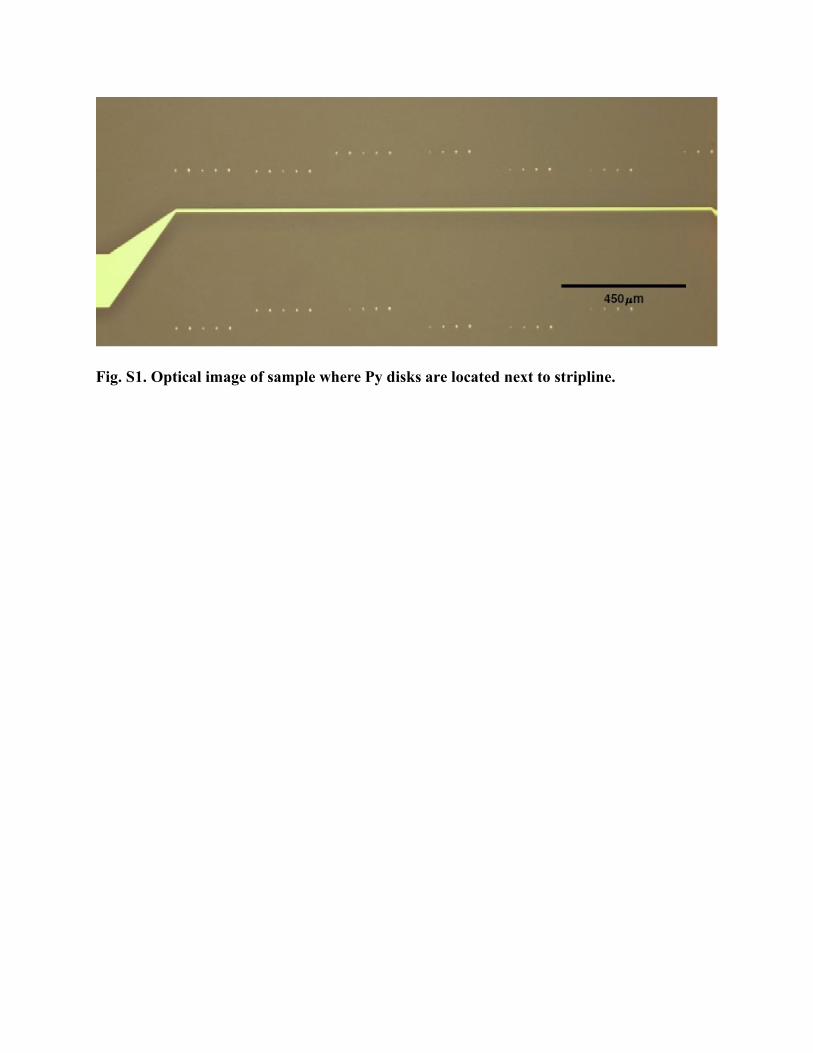
Fig. S1. Optical image of sample where Py disks are located next to stripline.

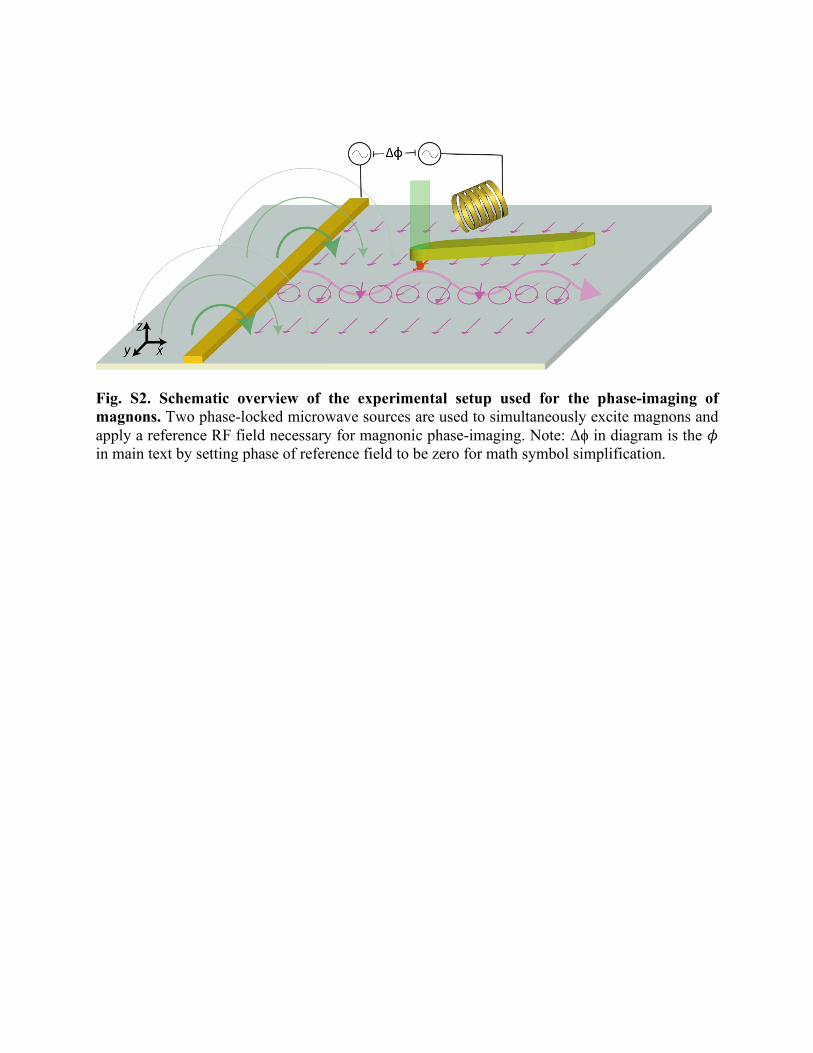
Fig. S2. Schematic overview of the experimental setup used for the phase-imaging of magnons. Two phase-locked microwave sources are used to simultaneously excite magnons and apply a reference RF field necessary for magnonic phase-imaging. Note: Δϕ in diagram is the 𝜙𝜙 in main text by setting phase of reference field to be zero for math symbol simplification.

Fig. S3. Simulated Fourier spectrum of the RF field that is used to excite magnons in the YIG. Fourier transform of the numerically simulated spatial profile of the x and z component of the microstrip magnetic field. The inset shows the actual magnetic field profiles.

0 1 2 3 4 5

k (rad/ m)

0.5

1FT

am

plitu

de (a

.u.)

Bx

Bz

-100 -50 0 50 100

x ( m)

-0.5

0

0.5

1

BR

F (a

.u.)

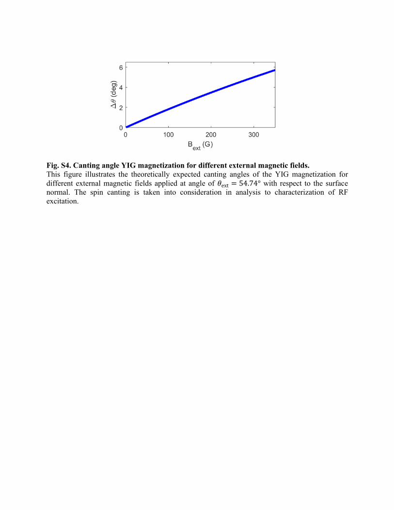
Fig. S4. Canting angle YIG magnetization for different external magnetic fields. This figure illustrates the theoretically expected canting angles of the YIG magnetization for different external magnetic fields applied at angle of 𝜃𝜃ext = 54.74° with respect to the surface normal. The spin canting is taken into consideration in analysis to characterization of RF excitation.

Fig. S5. Magnon dispersion near the NV spin transition. Schematic illustration of the magnon dispersion near the ESR transition of the NV center. The colored area represents the magnon dispersion plane, which depends both on the wavevector k and the external magnetic field 𝐵𝐵ext. The shading indicates the efficiency at which the magnons are excited by the microwave field, which is proportional by its Fourier amplitude (red and magenta lines). The ESR transition of the NV center is indicated by the blue plane. The blue line highlights the crossing between the NV spin transition and the magnon transition and indicates the magnons probed by our sensor.

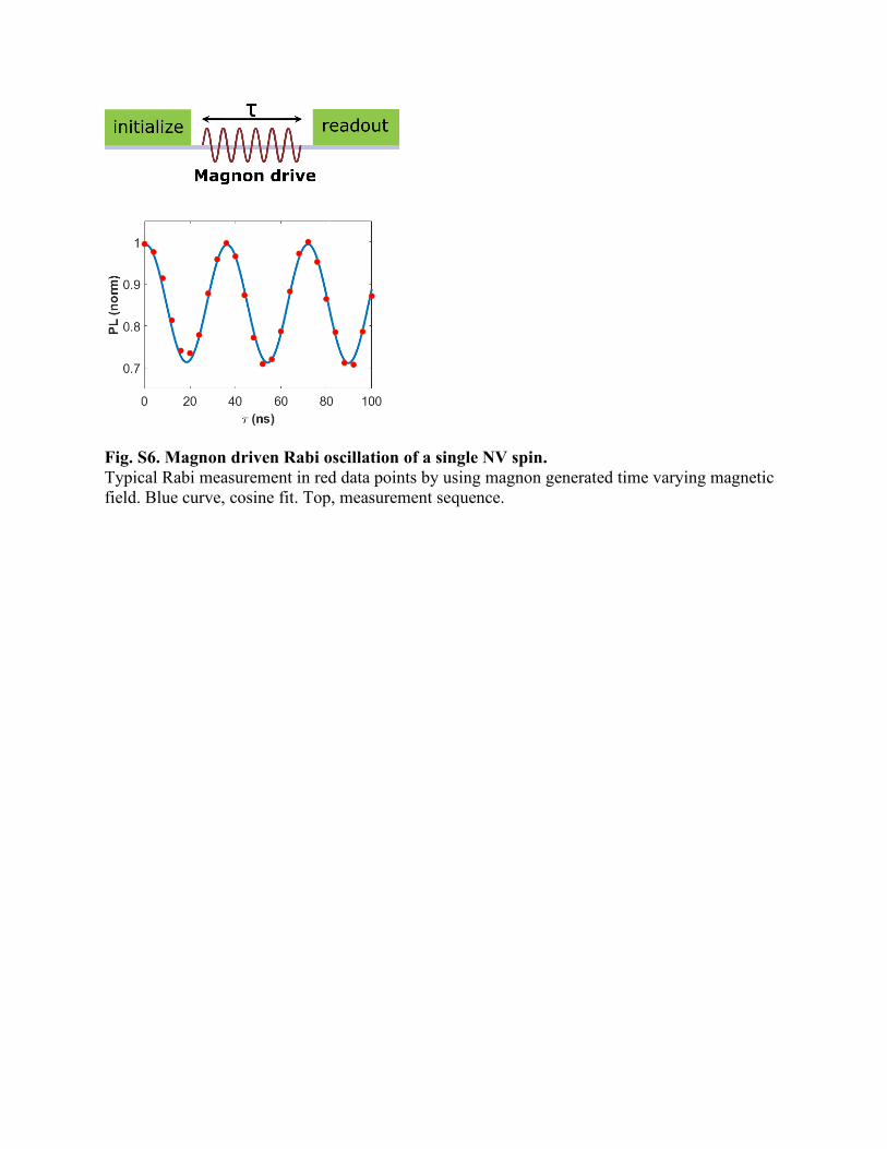
Fig. S6. Magnon driven Rabi oscillation of a single NV spin. Typical Rabi measurement in red data points by using magnon generated time varying magnetic field. Blue curve, cosine fit. Top, measurement sequence.

Fig. S7. Damon-Eshbach geometry for the analysis of surface magnetostatic waves in a magnetic thin film. Here 𝑑𝑑 is the film thickness and 𝐻𝐻0 is that static bias field.

Fig. S8. Convergence of the error during the Nelder-Mead simplex search of Hermite polynomial target functions Blue line shows the minimization of the error for a single dipolar source, i.e. all 𝑎𝑎𝑚𝑚𝑚𝑚 are zero excepts 𝑎𝑎01. After the convergence to the optimal parameters, we add additional components to the target and use the previously obtained parameters as initial staring point. Adding 𝑎𝑎00 and 𝑎𝑎10 results in improved accuracy, as indicated by the red line. The green curve shows the error when optimizing with all components up to 𝑎𝑎44. Note that the typical variance per pixel is 5.5.

Fig. S9. Scattering theory for disk shaped targets (A) Best fit for 𝐼𝐼𝑝𝑝, as given by Eq. S43, for a sharp disk-shaped target. The source functions are shown in Fig. S11. (B) Best fit for 𝐼𝐼𝑝𝑝, as given by Eq. S43, for a smoothened disk-shaped target, i.e. the disk is convoluted with a Gaussian that is 3 times larger than in panel (A) and (C). (C) The associated amplitude scan 𝐼𝐼𝑎𝑎, for the same sharp disk as in (A). (D) Amplitude scan 𝐼𝐼𝑎𝑎 for the smoothened disk. All sources are shown in Fig. S11.

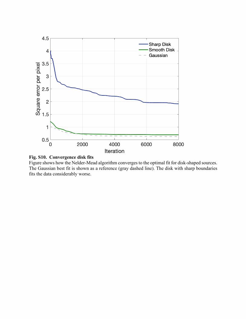
Fig. S10. Convergence disk fits Figure shows how the Nelder-Mead algorithm converges to the optimal fit for disk-shaped sources. The Gaussian best fit is shown as a reference (gray dashed line). The disk with sharp boundaries fits the data considerably worse.

Fig. S11. Disk shaped targets Fitted target functions for disk-shaped basis functions. (A-B) Shows the real and imaginary part of the optimal fit with a sharp disk; corresponding to Fig.S9 (A-C) (C-D) Shows the real and imaginary part of the optimal fit with a smooth disk; corresponding to Fig.S9 (B-D). The smooth disk is obtained by convolving the sharp disk with a Gaussian width a standard deviation of 800nm.

References 1. Maletinsky, P. et al. A robust scanning diamond sensor for nanoscale imaging with single

nitrogen-vacancy centres. 7, (2012).

2. Zhou, T. X., Stöhr, R. J. & Yacoby, A. Scanning diamond NV center probes compatible with

conventional AFM technology. Applied Physics Letters 111, (2017).

3. Xie, L., Zhou, T. X., Stöhr, R. J. & Yacoby, A. Crystallographic Orientation Dependent

Reactive Ion Etching in Single Crystal Diamond. 1705501, 1–6 (2018).

4. Prabhakar, A. & Stancil, D. D. Spin waves, Theory and application. (Springer US, 2009).

doi:https://doi.org/10.1007/978-0-387-77865-5.

5. Li, Y. Novel torques on magnetization measured through ferromagnetic resonance. Thesis

(2015).

6. Yu, H. et al. Magnetic thin-film insulator with ultra-low spin wave damping for coherent

nanomagnonics. Scientific Reports 4, 2–6 (2014).

7. Gruszecki, P., Kasprzak, M., Serebryannikov, A. E., Krawczyk, M. & Smigaj, W.

Microwave excitation of spin wave beams in thin ferromagnetic films. Scientific Reports 6,

1–8 (2016).

8. Andrich, P. et al. Long-range spin wave mediated control of defect qubits in nanodiamonds.

npj Quantum Information 3, 28 (2017).

9. Kikuchi, D. et al. Long-distance excitation of nitrogen-vacancy centers in diamond via

surface spin waves. Applied Physics Express 10, (2017).

10. Kalinkos, B. A. & Slavin, A. N. Theory of dipole-exchange spin wave excitation for

ferromagnetic films with mixed exchange boundary conditions. International Magnetics

Conference BP13–BP13 (1989) doi:10.1109/INTMAG.1989.690039.

11. Lim, J., Bang, W., Trossman, J., Amanov, D. & Ketterson, J. B. Forward volume and surface

magnetostatic modes in an yttrium iron garnet film for out-of-plane magnetic fields: Theory

and experiment. AIP Advances 8, (2018).

12. Casola, F., van der Sar, T. & Yacoby, A. Probing condensed matter physics with

magnetometry based on nitrogen-vacancy centres in diamond. Nature Reviews Materials 3,

17088 (2018).

13. Dovzhenko, Y. & Yacoby, A. Magnetostatic twists in room-temperature skyrmions explored

by nitrogen-vacancy center spin texture reconstruction. Nature Communications 1–7 (2018)

doi:10.1038/s41467-018-05158-9.

14. Landau, L. & Lifshitz, E. 3 - On the theory of the dispersion of magnetic permeability in

ferromagnetic bodies Reprinted from Physikalische Zeitschrift der Sowjetunion 8, Part

2, 153, 1935. in Perspectives in Theoretical Physics (ed. Pitaevski, L. P.) 51–65 (Pergamon,

1992). doi:10.1016/B978-0-08-036364-6.50008-9.

15. Damon, R. W. & Eshbach, J. R. Magnetostatic modes of a ferromagnet slab. Journal of

Physics and Chemistry of Solids 19, 308–320 (1961).

16. Hurben, M. J. & Patton, C. E. Theory of magnetostatic waves for in-plane magnetized

anisotropic films. Journal of Magnetism and Magnetic Materials 163, 39–69 (1996).

17. Tamaru, S., Bain, J. A., Kryder, M. H. & Ricketts, D. S. Green’s function for magnetostatic

surface waves and its application to the study of diffraction patterns. Phys. Rev. B 84,

064437 (2011).