DDRRAAFFTT
Stock Assessment for the West Coast Rock
Lobster Fishery
This information is distributed solely for the purpose of pre-dissemination peer review.
It has not been formally disseminated by the Department of Fisheries. It does not
represent any final agency determination or policy.
(23/09/2008)
This has been provided to invited Western Rock Lobster Stock Assessment and Harvest
Strategy Workshop participants
Nick Caputi, Roy Melville-Smith, Simon de Lestang, Jason
How, Adrian Thomson, Peter Stephenson, Ian Wright, and
Kevin Donohue

Table of Contents
DDRRAAFFTTTable of Figures........................................................................................... x
List of Boxes.............................................................................................. xv
List of Plates ............................................................................................. xvi
List of Tables ............................................................................................ xvi
Acknowledgements ................................................................... xviii
Executive Summary..................................................................... xix
Background................................................................................. xxii
1 – The Fishery ............................................................................... 1
1.1 – Overview ............................................................................................ 1
1.2 – Commercial Fishery ........................................................................... 3
1.3 – Recreational Fishery........................................................................... 4
1.4 – Illegal Catch........................................................................................ 5
1.4.1 – Illegal fishing activities................................................................................... 5
1.4.2 – Taxation considerations .................................................................................. 7
2 – Management ............................................................................. 8
2.1 – Management Objective....................................................................... 8
2.2 – History of Commercial Management Regulations............................. 9
2.3 – Boundaries and Zoning .................................................................... 11
2.4 – Current Management Strategies ....................................................... 13
This is a DRAFT and information is solely for pre-dissemination peer review i

2.4.1 Recreational Specific Management Strategies................................................. 14
DRAFTDRAFT2.5 – Marine Stewardship Council (MSC) Certification .......................... 15
2.6 – Integrated Fisheries Management (IFM).......................................... 16
3 – Biology ................................................................................... 17
3.1 – Taxonomy......................................................................................... 17
3.2 – Stock Structure ................................................................................. 19
3.3 – Habitats............................................................................................. 20
3.2.1 – Oceanography ............................................................................................... 20
3.2.2 – Physical Habitat ............................................................................................ 22
3.4 – Life History ...................................................................................... 23
3.5 – Movement......................................................................................... 28
3.5.1 – Migration....................................................................................................... 28
3.5.2 – Foraging ........................................................................................................ 29
3.6 – Reproduction .................................................................................... 30
3.6.1 – Size at maturity ............................................................................................. 31
3.6.2 – Spawning Season .......................................................................................... 38
3.6.3 – Fecundity....................................................................................................... 39
3.7 – Juvenile Recruitment........................................................................ 41
3.8 – Age and Growth ............................................................................... 42
3.8.1 – Methods......................................................................................................... 42
3.9 – Diet ................................................................................................... 48
4 – Fisheries Time Series Data ..................................................... 49
This is a DRAFT and information is solely for pre-dissemination peer review ii
4.1 – Puerulus ............................................................................................ 49
DDRRAAFFTT4.1.1 – Methods......................................................................................................... 49
Location ................................................................................................................ 49
Puerulus collectors ............................................................................................... 51
Puerulus Settlement Monitoring ........................................................................... 53
Analysis ................................................................................................................. 54
4.1.2 – Results........................................................................................................... 55
4.2 – Commercial Monitoring ................................................................... 58
4.2.1 – Methods......................................................................................................... 58
Location ................................................................................................................ 58
Sampling ............................................................................................................... 58
Analysis ................................................................................................................. 60
Fishery-Dependent Breeding Stock Index..................................................................................60
Biological Reference Points .......................................................................................................61
Index of Juvenile Abundance .....................................................................................................61
4.2.2 – Results........................................................................................................... 62
Fishery-Dependent Breeding Stock Index..................................................................................62
Index of Juvenile Abundance .....................................................................................................62
4.3 – Independent Breeding Stock Survey (IBSS).................................... 65
4.3.1 – Methods......................................................................................................... 65
Sampling Locations............................................................................................... 65
Breeding Stock Sampling Regime ......................................................................... 67
Tagging ................................................................................................................. 67
Analysis ................................................................................................................. 69
Fishery Independent Breeding Stock Index (BSI)......................................................................69
This is a DRAFT and information is solely for pre-dissemination peer review iii
4.3.2 – Results........................................................................................................... 70
Fishery Independent Breeding Stock Index (BSI)......................................................................70
DDRRAAFFTT4.4 – Volunteer Research Log Books........................................................ 72
4.4.1 – Methods......................................................................................................... 72
4.4.2 – Results........................................................................................................... 73
4.5 – Catch and Effort Statistics (CAES).................................................. 77
4.5.1 – Methods......................................................................................................... 78
4.6 – Processor Returns ............................................................................. 79
4.6.1 – Methods......................................................................................................... 79
4.7 – Environmental Data.......................................................................... 81
4.7.1 – Methods......................................................................................................... 81
Rainfall.................................................................................................................. 81
Sea Level ............................................................................................................... 81
Reynolds Satellite Sea Surface Temperatures....................................................... 81
Southern Oscillation Index (SOI).......................................................................... 82
4.7.2 – Results........................................................................................................... 82
Southern Oscillation Index (SOI).......................................................................... 82
4.8 – Recreational Fishery and Surveys .................................................... 84
4.8.1 – Methods......................................................................................................... 84
Mail Surveys.......................................................................................................... 84
Telephone Diary Surveys ...................................................................................... 87
Boat Ramp Survey................................................................................................. 87
4.8.2 – Results........................................................................................................... 88
Mail survey response rate..................................................................................... 88
This is a DRAFT and information is solely for pre-dissemination peer review iv

Comparisons of survey techniques........................................................................ 89
Effort ..................................................................................................................... 91
DDRRAAFFTTCatch Rates ........................................................................................................... 94
5 – Stock Assessment ................................................................... 95
5.1 Fishing Efficiency ............................................................................... 95
5.1.1 – Methods......................................................................................................... 95
Changes in gear and technology........................................................................... 95
Soak Time ..................................................................................................................................96
Pot Type .....................................................................................................................................96
5.1.2 – Results........................................................................................................... 96
Colour Sounders and GPS ..........................................................................................................96
Standardised Effort and Nominal Effort ............................................................... 97
5.2 – Catch Prediction ............................................................................... 99
5.2.1 – Methods......................................................................................................... 99
Commercial Catch Prediction .............................................................................. 99
Recreational Catch and Effort Prediction .......................................................... 101
5.2.2 – Results......................................................................................................... 102
Commercial Catch Prediction ............................................................................ 102
Recreational Catch Prediction ........................................................................... 103
5.3 – Stock Recruitment-Environment Relationship (SRR) and
Recruitment to Spawning Stock Relationship (RSR) ............................. 104
5.3.1 – Methods....................................................................................................... 104
5.3.2 – Results......................................................................................................... 105
Stock Recruitment-Environment Relationship .................................................... 105
This is a DRAFT and information is solely for pre-dissemination peer review v

Recruitment to Spawning Relationship............................................................... 106
5.3.3 –Discussion .................................................................................................... 106
DDRRAAFFTT5.4 – Depletion Analysis ......................................................................... 107
5.4.1 - Methods ....................................................................................................... 107
Assumptions and some consequences ................................................................. 110
Environmental influence on catchability ............................................................ 111
Optimal Estimation of Underlying Trend. .......................................................... 114
Centred Moving Average Estimate ..........................................................................................114
Optimal Combinations of Estimators.................................................................. 114
Weighted Moving Average Smoothing of time series data. .....................................................114
Cycles in moving average smoothed series. .............................................................................115
Diagnostics for Depletion Model Validity .......................................................... 116
Depletion based estimates for fishery harvest .................................................... 116
Depletion based estimates for residual biomass................................................. 116
5.4.2 – Results......................................................................................................... 117
Harvest trends in Zone A .................................................................................... 117
Harvest trends in Zone B .................................................................................... 117
Harvest trends in Zone C .................................................................................... 118
5.5 – Biological Modelling...................................................................... 122
5.5.1 – Methods....................................................................................................... 124
Population dynamics model................................................................................ 124
Recruitment ..............................................................................................................................124
Availability to capture ..............................................................................................................126
Egg Production .........................................................................................................................128
Catches .....................................................................................................................................129
This is a DRAFT and information is solely for pre-dissemination peer review vi

Data sources ....................................................................................................... 129
Catch and effort ........................................................................................................................129
DDRRAAFFTTPuerulus data ............................................................................................................................129
Setose lobsters ..........................................................................................................................132
Objective function ....................................................................................................................132
Parameter values ................................................................................................ 133
Parameters assumed..................................................................................................................133
5.5.2 – Results......................................................................................................... 134
Catch estimation ................................................................................................. 134
Model derived breeding stock indices................................................................. 135
5.5.3 – Assessment of proposal management changes for the 2008/09 – 2010/11
fishing seasons ........................................................................................................ 137
Background ......................................................................................................... 137
Impact of effort reduction scenarios on commercial catch ................................ 137
Northern coastal zone (B)................................................................................... 137
Southern coastal zone (C)................................................................................... 139
Impact of effort reduction scenarios on breeding stock levels ........................... 140
Northern coastal zone (B)................................................................................... 140
Southern coastal zone (C)................................................................................... 141
5.5.4 – Future Directions ........................................................................................ 142
5.6 – Economic Model ............................................................................ 143
5.6.1 – Methods....................................................................................................... 143
Pot Reductions .................................................................................................... 143
Time Closures ..................................................................................................... 144
Maximum Female Size Reduction....................................................................... 144
This is a DRAFT and information is solely for pre-dissemination peer review vii

5.6.2 – Results......................................................................................................... 144
Pot Reductions .................................................................................................... 146
DDRRAAFFTTTime Closures ..................................................................................................... 146
Maximum Female Size Reduction....................................................................... 146
Management Package Outcome ......................................................................... 146
5.6.3 – Future Direction .......................................................................................... 147
6 – Biological Reference Points and Stock Status...................... 148
6.1 – Management Decision Framework ................................................ 148
6.1.1 – Background ................................................................................................. 148
6.1.2 – Decision Rules ............................................................................................ 149
6.1.3 –Future Direction ........................................................................................... 150
6.2 – Stock Status .................................................................................... 151
6.2.1 – Stock Status by Zone (2005/06 fishing season).......................................... 152
Zone A ................................................................................................................. 152
Zone B ................................................................................................................. 153
Zone C................................................................................................................. 154
7 – Current Research .................................................................. 155
7.1.1 – Reproductive Biology Pertinent to Brood Stock Management................... 155
7.1.2 – Lobster Movement Through Acoustic Tracking......................................... 155
7.1.3 – Effects of Closed Areas .............................................................................. 156
7.1.4 – Climate Change........................................................................................... 157
8 – Recommendations for Future Research................................ 158
This is a DRAFT and information is solely for pre-dissemination peer review viii
9 – References ............................................................................ 159
DRAFTDRAFT10 – Appendixes ......................................................................... 168
Appendix 1 – Header sheet used to record all ancillary data collected during the
commercial monitoring program ............................................................................ 168
Appendix 2 – Data recording sheet for the IBSS, showing information recorded. 169
Appendix 3 – Voluntary logbook filled in by commercial fishers.......................... 170
Appendix 4 – CAES logbook showing the data recorded by fishers monthly ....... 171
Appendix 5 – Forms filled out by rock lobster processors a) log of fisherman and
catch for that month, and b) breakdown of product and grades of exported or sold
domestically. ........................................................................................................... 172
Appendix 6 – Mail survey (1997/98 season) representative of those sent pre 1998
................................................................................................................................. 173
Appendix 7 – Mail survey sent out in 1999, reflective of the more recent, detailed
mail surveys ............................................................................................................ 174
Appendix 8 – Location map used in the phone diary survey.................................. 175
Appendix 9 – Decision rule framework from Bray (2004)..................................... 180
This is a DRAFT and information is solely for pre-dissemination peer review ix

Table of Figures
DDRRAAFFTTFigure 1.1 – Distribution of the Western Rock Lobster Panulirus cygnus......................... 1
Figure 1.2 – Annual catch, effort and total allowable effort (TAE) for Panulirus cygnus in
the WCRLMF. ............................................................................................................ 2
Figure 1.3 – Two main trap types used by lobster fishers and their associated size and
configuration regulations a) batten design (made of wood); b) cane beehive pot
(details of pot regulations; Box 2.1 and 2.2)............................................................... 3
Figure 1.4 – Catch of the western rock lobster fishery from fishers’ monthly returns, and
that adjusted for illegal activities and under reporting (adapted from Caputi et al.
2000). .......................................................................................................................... 7
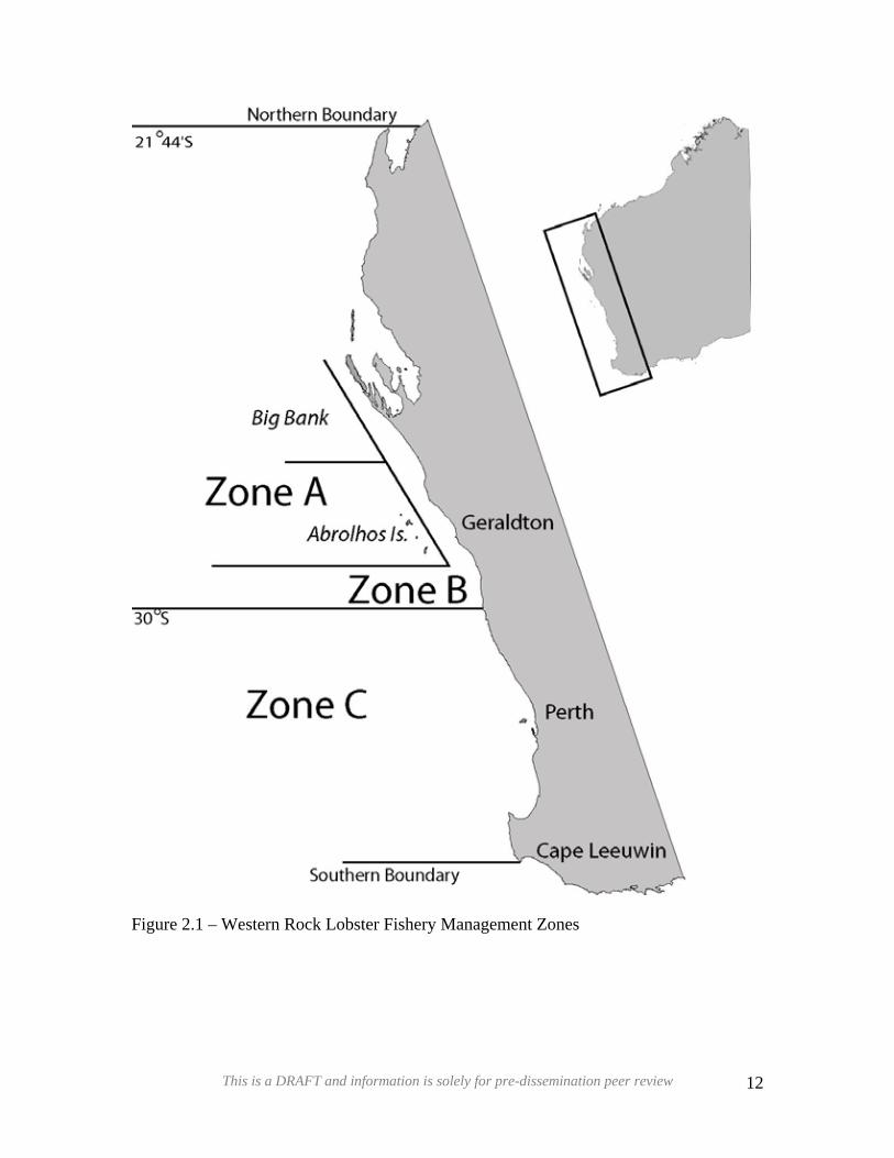
Figure 2.1 – Western Rock Lobster Fishery Management Zones .................................... 12
Figure 3.1 – Distribution of Palinuridae (spiny) lobsters around Australia...................... 17
Figure 3.2 - Morphology of the Panulirus cygnus showing where the carapace
measurement is taken and variation in male and female morphology...................... 18
Figure 3.3 – Distribution of phyllosoma western rock lobster larvae (from Phillips 1981)
................................................................................................................................... 25
Figure 3.4 – Life history of Panulirus cygnus (from Community Education Branch (CEB,
Department of Fisheries, Western Australia)............................................................ 27
Figure 3.5 – Logistic regressions fitted to the percentage of mature female Panulirus
cygnus at different carapace lengths in six locations in Western Australia, based on
data collected during the 2002 Independent Breeding Stock Survey. CL50±1 SE
denotes the size at which 50% of the assemblage is mature and n the sample size
(Melville-Smith & de Lestang 2006)........................................................................ 32
Figure 3.6 – Relationship between the merus length of the second pereiopod and carapace
length of immature (open circle) and mature (filled circle) male Panulirus cygnus
(left) and logistic regressions fitted to the percentage of morphometrically mature
males at different carapace lengths (right) in six locations in Western Australia,
This is a DRAFT and information is solely for pre-dissemination peer review x
DDRRAAFFTTbased on data collected during the 2002 Independent Breeding Stock Survey.
CL50±1 SE denotes the size at which 50% of the assemblage is mature and n the
sample size (Melville-Smith & de Lestang 2006)..................................................... 33
Figure 3.7 – a) Size at maturity (CL50) ±1 SE of female (filled circle) and male (open
circle) Panulirus cygnus at six locations and b) linear regressions fitted to the
relationships between female (filled circle) or male (open circle) CL50s at each
location and the corresponding mean annual water temperature at that location
(Melville-Smith & de Lestang 2006). ....................................................................... 34
Figure 3.8 – Temporal variation in size at maturity (CL50) ±1 SE of female Panulirus
cygnus at six locations from the early 1990s to mid-2000s from IBSS surveys, with
the vertical line representing 1994 (Melville-Smith & de Lestang 2006). ............... 36
Figure 3.9 – Mean carapace lengths of the smallest 10% of mature female Panulirus
cygnus caught in each year at four locations from 1972 to 2005 based on data
collected during Fishery Dependent Commercial Catch Monitoring (filled circle)
and from 1992 to 2005 based on data collected during Fishery Independent Breeding
Stock Surveys (open circle). Horizontal dotted line represents 76 mm and dashed
line represents a linear regression between mean carapace length and the years
before 1986 (Melville-Smith & de Lestang 2006).................................................... 37
Figure 3.10 – Monthly catch rates of berried females (number per pot lift) (Adapted from
Chubb 1991).............................................................................................................. 38
Figure 3.11 – Fecundity of Panulirus cygnus compared to carapace length (CL). .......... 39
Figure 3.12 – Probability at double breeding at five coastal locations and the Abrolhos
Islands (de Lestang & Melville-Smith 2006)............................................................ 40
Figure 3.13 – Single moult growth increments for female lobsters at Dongara with a
logistic function fitted through the distribution. Figures on the left represent the
growth increment estimated for the November moult for lobsters in their first (A) to
fifth (I) year after release, while those on the right represent the growth increment
over the March moult for lobsters released for the same periods of time (Stephenson
and de Lestang in prep)............................................................................................. 44
This is a DRAFT and information is solely for pre-dissemination peer review xi
Figure 3.14 – Example of the modelled growth curves showing the median and 95% CI
of a) female and, b) male western rock lobster at Dongara. ..................................... 47
DRAFTDRAFTFigure 4.1 – Location of current (2007) puerulus collector sites...................................... 50
Figure 4.2 – Average puerulus settlement by month for sites in the northern (Dongara),
southern (Lancelin) and offshore (Abrolhos Islands) zones of the WRL fishery..... 55
Figure 4.3 – Average month of peak puerulus settlement from current (2007) puerulus
collectors throughout the WRL fishery..................................................................... 56
Figure 4.4 – Puerulus numbers per collector for each season at collector sites throughout
the fishery.................................................................................................................. 57
Figure 4.5 – Locations of commercial monitoring sites ................................................... 59
Figure 4.6 – Fishery-dependent spawning stock indices for the a) northern (Zone B) and
b) southern (Zone C) regions of the fishery with a 3-year moving average.
Biological Reference Point (BRP) for each area is shown (green line).................... 63
Figure 4.7 – Juvenile indices for the northern and southern regions, adjusted for escape
gap changes in 1986/87 and fishing efficiency. a) Lobsters <68 mm CL and b)
juveniles 68-76 mm CL. ........................................................................................... 64
Figure 4.8 – Location of independent breeding stock survey (IBSS) sites sampled
annually (yellow diamond) and every five years (white diamond). ......................... 66
Figure 4.9 – IBSS indices (± 1 SE) and three year moving average (thick line) for; a)
Zone A; b) Zone B and; c) Zone C ........................................................................... 71
Figure 4.10 – Average number of vessels that returned logbooks for each block in seasons
1986/87 through to and including 2005/06. .............................................................. 74
Figure 4.11 – Number of vessels that returned logbooks for each block in the 2005/06
season........................................................................................................................ 75
Figure 4.12 – Daily catch rate of coastal sites for last three seasons (2003/04 – 2005/06)
................................................................................................................................... 76
This is a DRAFT and information is solely for pre-dissemination peer review xii
Figure 4.13 – Weight of setose females returned by fishers each season since 1992/93 in
each region of the fishery.......................................................................................... 76
DDRRAAFFTTFigure 4.14 – Mean sea level for Fremantle (black), and the Southern Oscillation Index
(red), puerulus settlement (green) showing the effects of El Niño events (yellow
blocks) (Updated from Pearce & Phillips 1988)....................................................... 83
Figure 4.15 – Map codes for regions of licence holder residence and fishing effort
(Melville-Smith & Anderton 2000). ......................................................................... 86
Figure 4.16 – Return rates in recreational lobster fisher mail survey. (open triangles and
dashed line indicates estimated return rates from the 1998/89 survey). Thick line
indicates period where inducements (with or without reminders) were offered, with
the thin line being when only reminders were sent................................................... 88
Figure 4.17 - Recreational catch estimates based on ‘raw estimates’ from the mail survey
(black) and the adjusted estimates calculated from the ‘phone diary based’ correction
factor (red). The forecast recreational catches for 2007/08 to 2008/09 are based on
puerulus settlement levels for the period 2004to 2006 (IFAAC 2007). ................... 91
Figure 4.18 – Average number of days fished per month by recreational lobster pot and
dive fishers who reported fishing in the 1998/99 survey (Melville-Smith & Anderton
2000). ........................................................................................................................ 92
Figure 4.19 – Number of days fished by month from the phone/diary survey for the four
seasons surveyed (Updated from IFAAC 2007). ...................................................... 92
Figure 4. 20 – Location of residence and fishing for lobster licence holders (Melville-
Smith & Anderton 2000) .......................................................................................... 93
Figure 4.21 – The proportion (%) recreational catch for a zone compared with the total
lobster catch in that zone (zones A/B and Zone C; using adjusted recreational catch
estimates). The forecast percentages (dotted lines) are based on the expected
commercial and recreational catches for the next three seasons (2004/05 to 2006/07).
Note the recreational catch in Zone A is minimal and is included in Zone B (IFAAC
2007). ........................................................................................................................ 94
Figure 5.1 – Standardised and nominal fishing effort in the WRL fishery....................... 98
This is a DRAFT and information is solely for pre-dissemination peer review xiii
Figure 5.2 – Predicted catch (dotted line) and the actual catch (solid lines) for three
management zones of the WRL commercial fishery. ............................................. 102
DDRRAAFFTTFigure 5.3 – Model predictions of recreational catch (open circle), with 95% CI (bars),
with actual catches (solid circles) for season to 2002/3 Melville-Smith et al. (2004).
................................................................................................................................. 103
Figure 5.4 – Actual and Bayesian estimates catch per unit effort (CPUE) per month
(March–June) plotted against the cumulative catch index for a number of years for:
A, Zone A; and B, Zone C. Note that for the Zone C depletions for 1999 and 2001
on, the March and June CPUE values respectively have been omitted for biological
reasons explained in the text (Wright et al. 2006). ................................................. 110
Figure 5.5 – Estimates of residual biomass, harvest rate and catchability estimates (±SD)
from the depletion analysis for Zone A, with a modified three-point smoothed
average (adapted from Wright et al. (2006)............................................................ 119
Figure 5.6 – Estimates of residual biomass, harvest rate and catchability estimates (±SD)
from the depletion analysis for Zone B, with a modified three-point smoothed
average (adapted from Wright et al. (2006)............................................................ 120
Figure 5.7 – Estimates of residual biomass, harvest rate and catchability estimates (±SD)
from the depletion analysis for Zone C, with a modified three-point smoothed
average (adapted from Wright et al. (2006)............................................................ 121
Figure 5.8 – Map of lower West Australian coast showing finer scale grids used in the
modelling of the western rock lobster..................................................................... 123
Figures 5.9 – Actual and modelled catches for the (a) northern and (b) southern coastal
regions of the fishery. ............................................................................................. 135
Figures 5.10 – Model-derived breeding stock indices (±SE) for a) northern and b)
southern coastal regions (both based on data from the deep-water regions of the
same areas as the dependent BSI, respectively). Observed values are fishery
dependent BSIs scaled to allow comparisons. ........................................................ 136
Figure 5.11 Model-derived impact of four-effort reduction scenarios on the predicted
commercial catches in the northern B zone. ........................................................... 139
This is a DRAFT and information is solely for pre-dissemination peer review xiv
Figure 5.12. Model-derived impact of four-effort reduction scenarios on the predicted
commercial catches in the southern C zone. ........................................................... 140
DRAFTDRAFTFigure 5.13. Model-derived impact of four-effort reduction scenarios on the predicted
breeding stock index in the northern B zone. ......................................................... 141
Figure 5.14. Model-derived impact of four-effort reduction scenarios on the predicted
breeding stock index in the southern C zone. ......................................................... 142
Figure 5.15 – Expected gross margin in year 1 versus the effective effort reduction for
Zone B (Thomson & Caputi 2006) ......................................................................... 145
Figure 5.16 – Expected gross margin in year 2 versus the effective effort reduction for
Zone B (Thomson & Caputi 2006). ........................................................................ 145
Figure 6.1 – Variation in WRL breeding stock abundance as a percentage of unfished
biomass over time in relation to two biological reference points, the 1980 level
(BRP) and 20% below this level (BRP20) (Bray 2004). The two BRP represent
different levels of management action required...................................................... 149
Figure 6.2 – Proposed new model assessing the stock vulnerability based on breeding
stock and harvest rate levels. .................................................................................. 150
List of Boxes
Box 2.1 – Timeline of major management regulatory changes introduced into the
WCRLMF. .................................................................................................................. 9
Box 2.2 – Summary of current (2006/07) WRL Management Arrangements (adapted
from Caputi et al. 2000) ............................................................................................ 13
This is a DRAFT and information is solely for pre-dissemination peer review xv

List of Plates
DDRRAAFFTTPlate – 3.1 - Thermal image showing the warm water of the Leeuwin Current (red and
orange and yellow) flowing southwards and it’s associated eddies.
(http://www.cmar.csiro.au/remotesensing/AlanPearce/regional/index.html)........... 21
Plate 3.2 – Ventral view of a) male WRL, b) female WRL, c) tar-spotted female and d)
berried female ........................................................................................................... 24
Plate 3.3 – Life phases of the Panulirus cygnus a) phyllosoma (TL 20mm); b) puerulus
(TL inc. outstretched antennae 35mm); c) juvenile (CL 7 – 9mm) .......................... 25
Plate 3.4 – Pleopods with a) no setae and b) mature setae. .............................................. 30
Plate 4.1 – Puerulus collectors a) design with two panels missing to show internal
construction and, b) retrieved from site before being “banged”............................... 51
Plate 4.2 – Collection of puerulus from collectors by a) shaking puerulus collector and b)
sieving contents......................................................................................................... 53
Plate 4.3 – Tagged lobster showing location and type of tag ........................................... 68
List of Tables
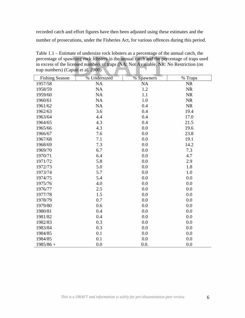
Table 1.1 – Estimate of undersize rock lobsters as a percentage of the annual catch, the
percentage of spawning rock lobsters in the annual catch and the percentage of traps
used in excess of the licensed numbers of traps (NA: Not Available, NR: No
Restriction (on trap numbers) (Caputi et al. 2000) ..................................................... 6
Table 3.1 – Proportion of three out of all three and four year post-puerulus lobsters in the
whites and reds catches at eight different locations throughout the fishery, estimated
from puerulus – catch relationships (de Lestang et al. in prep). ............................... 45
Table 4.1 – Location of historical and current puerulus collector sites and the number of
collectors at each site. ............................................................................................... 49
This is a DRAFT and information is solely for pre-dissemination peer review xvi
Table 4.2 – Puerulus collector locations and collectors used in the development of
puerulus settlement indices for the three management zones................................... 55
DRAFTDRAFTTable 4.3 – Processor grades for Panulirus cygnus showing the weight and carapace
length (CL) ranges. ................................................................................................... 79
Table 4.4 – Data recorded as part of the phone diary survey ........................................... 87
Table 4.5 – Comparison of different variable estimates using diary and mail survey data
for various seasons in which both methods were performed. Adapted from IFAAC
(2007)........................................................................................................................ 89
Table 4.6 - Different ratios for converting diary survey estimated total catch to that of the
mail survey. Ratios have been determined using a linear model with no intercept
using data for different seasons (indicated with a tick) (IFAAC 2007).................... 90
Table 5.1 – The annual percentage increase in fishing efficiency across all zones, for both
deep and shallow water, for fishing season from 1971/72........................................ 97
Table 5.2 - Covariances between log catchability (logq) and environmental variables
(temperature, salinity, pre-moult proportions (PMP) for data from Morgan (1974)
(Wright et al. 2006)................................................................................................. 112
Table 5.3 – Partial covariances between log catchability and temperature for Morgan
(1974) data with all other environmental variables held constant (Wright et al.
2006). ...................................................................................................................... 112
This is a DRAFT and information is solely for pre-dissemination peer review xvii

Acknowledgements
DDRRAAFFTTThe authors wish to thanks those that provided constructive reviews and information
critical to the production of this document. This includes Mark Rossbach, Eric Barker,
Tara Baharthah, Kris Waddington, Mark Cliff, Maree Apostoles, Eva Lai, Alan Pearce,
Sandy Clarke and Lynda Bellchambers. Also the Community Education Branch of the
Department of Fisheries for use of figures that were produced for the Naturaliste Marine
Discovery Centre.
Also the contribution of the Fisheries Research and Development Corporation should be
acknowledged for their support of many of the projects that are reported here
This is a DRAFT and information is solely for pre-dissemination peer review xviii
Executive Summary
DRAFTDRAFTThe western rock lobster Panulirus cygnus is exploited throughout its geographic range
along the lower west coast of Western Australia. The main commercial fishery exploiting
P. cygnus is the West Coast Rock Lobster Managed Fishery (WCRLMF). This is
Australia’s largest single species fishery worth $250 - $400 million annually. It is
important for the economy of a number of coastal towns along the west coast of Western
Australia. It also supports an important recreational fishery.
In 1963 the WCRLMF was declared a limited entry fishery, freezing pot and licence
numbers. Since that time the fishery has undergone a number of management changes
designed to maintain stock sustainability. Currently there are around 490 boats catching
on average of 11 million kg of western rock lobster. There is also an important
recreational fishery which has about 45, 000 licences issued annually. Recreational
fishing accounts for about 3% of the total catch of the fishery.
The WCRLMF was also the first fishery in the world to receive Marine Stewardship
Council Certification (MSC). In 2000, certification was given on the basis of it being a
sustainable fishery, and it was recertified in 2006. The ongoing accreditation requires the
addressing of criteria set by the MSC, which now also include considerable research
being undertaken on ecological impacts of the fishery.
The fishery is managed based on the status of the breeding stock relative to a threshold
Biological Reference Point (BRP), the 1980 level.
“Ensure the abundance of breeding lobsters is maintained or returned to, as the case
may be, at or above the levels in 1980.”
The commercial fishery is managed using a total allowable effort (TAE) system as well
as associated input controls. The primary control mechanism is the number of pot units,
together with a proportional usage rate, which creates the TAE in pot lifts. Unitisation in
the fishery and transferability provisions allow market forces to determine what is the
most efficient use of licences and pot entitlements, a system now known as individually
transferable effort (ITE). Management arrangements also include the protection of
females in breeding condition, a variable minimum carapace length and a maximum
This is a DRAFT and information is solely for pre-dissemination peer review xix

female carapace length and gear controls, including escape gaps and a limit on the
volume of pots.
DDRRAAFFTTThe western rock lobster is an omnivorous crustacean, found predominantly along the
mid and lower west coast of Western Australia in shallow and deep (> 100 m) reef
habitats. After a 9-11 month plankton phase taking them off the continental shelf, they
settle on shallow near-shore reefs (post larval phase - puerulus). Here they grow before
undergoing an offshore migration during the juvenile stage at about four to five years of
age, when they start to recruit to the fishery. Large and mature lobsters are mainly found
in deep water (>40m) breeding grounds.
Department of Fisheries researchers have ongoing program to monitor settlement of
puerulus, catches of the commercial fleet by onboard sampling and logbooks, the
breeding stock, recreational catches, and environmental conditions. This information is
used to assess changes in the stocks of the WRL, and form the basis of advice for
management decisions.
Stock assessment of the fishery is based on a number of empirical and modelled indices
that have been referred externally by stock assessment experts
(http://www.fish.wa.gov.au/docs/op/op050/fop050.pdf). These indices include:
o Trends in fishery-dependent breeding stock indices (current basis of threshold
biological reference point (BRP));
o Trends in puerulus settlement and understanding how these are affected by key
factors (e.g. Leeuwin Current);
o Catch prediction 3 – 4 years in advance;
o Depletion analysis providing trends in residual legal biomass and harvest rates;
o Biological model of the fishery that integrates information on recruitment, legal-
size lobsters and breeding stock.
The current state (30-June-2007) of the fishery in the three zones is as follows:
o The legal-size component of the stock in Zone A (Abrolhos Islands) is heavily
exploited. However its breeding component is well protected as much of it
matures before reaching legal size. It has achieved record catches in the last three
years.
This is a DRAFT and information is solely for pre-dissemination peer review xx
DDRRAAFFTTo The stock in Zone C (South Coastal) is moderately exploited and its breeding
component remains well above breeding stock threshold levels. This breeding
stock is considered healthy, although with four years of predicted low recruitment,
pre-emptive management (5% effort reduction in 2005/06) steps have been taken
to keep this stock above threshold levels.
o The stock in Zone B (North Coastal) is heavily exploited and its breeding
component is close to the breeding stock BRP threshold level. This stock is
considered vulnerable, and management changes have occurred (15% effort
reduction in 2005/06) to improve its status.
This is a DRAFT and information is solely for pre-dissemination peer review xxi

Background
DRAFTDRAFTThis draft document was initiated to provide a compendium of information for the stock
assessment of the West Coast Rock Lobster Fishery. It provides background information
for the expert panel reviewing the stock assessment for the fishery. As such, provides
information that will enable the reviews to examine:
i. The current western rock lobster stock assessment process and proposed future
research;
ii. A biological model that has recently been developed by the Department of
Fisheries (WA) for use in providing management advice for the western rock
lobster fishery and propose future directions for that work; and
iii. The current western rock lobster harvest strategy and recommend improvements
to it.
Once the reviewers’ comments have been received, the report will be revised and
provided to all stakeholders and made available publicly.
It should be noted, that this report does not deal with the social aspects of the fishery, or
the ecological interactions of the fishery. A separate process involving two scientific
reference groups (SRGs) (Sea Lion SRG and Ecosystem SRG) has been established and
meets regularly to deal with the ecological issues relating to the fishery.
This document is the first production of its type for the western rock lobster fishery. It is
a “living” document, with a synopsis of available biological information on Panulirus
cygnus, a guide to on going monitoring undertaken by the Department of Fisheries, and
an indication of the analyses leading to management decisions.
This document will be amended to reflect changes to procedures, and updated on a
regular basis.
This is a DRAFT and information is solely for pre-dissemination peer review xxii
1 – The Fishery
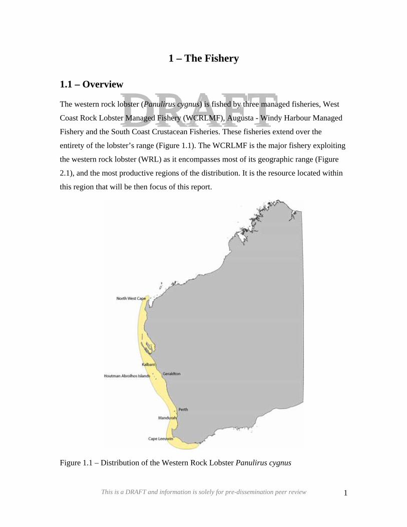
DRAFTDRAFTThe western rock lobster (Panulirus cygnus) is fished by three managed fisheries, West
Coast Rock Lobster Managed Fishery (WCRLMF), Augusta - Windy Harbour Managed
Fishery and the South Coast Crustacean Fisheries. These fisheries extend over the
entirety of the lobster’s range (Figure 1.1). The WCRLMF is the major fishery exploiting
the western rock lobster (WRL) as it encompasses most of its geographic range (Figure
2.1), and the most productive regions of the distribution. It is the resource located within
this region that will be then focus of this report.
1.1 – Overview
Figure 1.1 – Distribution of the Western Rock Lobster Panulirus cygnus
This is a DRAFT and information is solely for pre-dissemination peer review 1
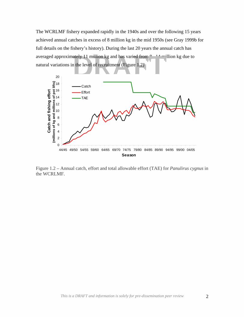
DDRRAAFFThe WCRLMF fishery expanded rapidly in the 1940s and over the following 15 years
achieved annual catches in excess of 8 million kg in the mid 1950s (see Gray 1999b for
full details on the fishery’s history). During the last 20 years the annual catch has
averaged approximately 11 million kg and has varied from 8 –14 million kg due to
natural variations in the level of recruitment (Figure 1.2) TT
0
2
4
6
8
10
12
14
16
18
20
44/45 49/50 54/55 59/60 64/65 69/70 74/75 79/80 84/85 89/90 94/95 99/00 04/05Season
Cat
ch a
nd fi
shin
g ef
fort
(mill
ions
of k
g an
d m
illio
ns o
f pot
lift
s)
Catch
EffortTAE
Figure 1.2 – Annual catch, effort and total allowable effort (TAE) for Panulirus cygnus in the WCRLMF.
This is a DRAFT and information is solely for pre-dissemination peer review 2
1.2 – Commercial Fishery
DDRRAAFFTTThe West Coast Rock Lobster Managed Fishery (WCRLMF) is the most valuable single-
species wild capture fishery in Australia (with the catch worth between $A250 and
$A400 million annually), representing about twenty per cent of the total value of
Australia’s wild capture fisheries.
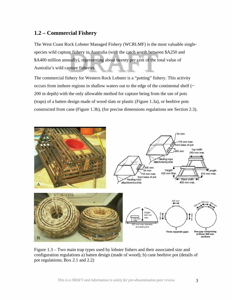
The commercial fishery for Western Rock Lobster is a “potting” fishery. This activity
occurs from inshore regions in shallow waters out to the edge of the continental shelf (~
200 m depth) with the only allowable method for capture being from the use of pots
(traps) of a batten design made of wood slats or plastic (Figure 1.3a), or beehive pots
constructed from cane (Figure 1.3b), (for precise dimensions regulations see Section 2.3).
Fcp
A
Bigure 1.3 – Two main trap types used by lobster fishers and their associated size and onfiguration regulations a) batten design (made of wood); b) cane beehive pot (details of ot regulations; Box 2.1 and 2.2)
This is a DRAFT and information is solely for pre-dissemination peer review 3
DDRRAAFFTTBaited pots are released (set) from boats near reefs where the lobsters usually reside or in
regions (usually sandy bottom) thought to be on migration paths during the migration
period. This is based upon a combination of information gained from depth sounders,
GPS systems, previous experience and recent catch rates in the area. The pots are left
overnight during which time lobsters are attracted to the baits and enter the pots. The pots
are generally retrieved (pulled) the following morning, though sets of multiple days (2 or
more days) do often occur, particularly during low catch rate periods. Captured lobsters
of legal size and of appropriate reproductive status (e.g. not setose etc.) are placed into
holding tanks and returned to on-shore processing plants where the majority are prepared
for overseas markets, many as live shipments.
The rock lobster fishery was declared limited entry in March 1963 when licence and pot
numbers were frozen. Since 1963, boat numbers have declined due to management
changes (pot reductions etc.) from 836 to 495 (May 2007). Vessels are currently
operating an average of 113 pots (2005/06). The record catch of 14,500 tonnes in the
1999/2000 season, was the second largest catch of any single species of rock lobster after
Panulirus argus.
1.3 – Recreational Fishery
This fishery also supports a significant recreational fishery with about 45,000 rock lobster
licences issued annually, around 80% of these being utilised, and catch approximately
400 tonnes per year (approx. 3% of the total commercial and recreational catch) (Section
4.8). Recreational fishers can catch WRL with pots (limit of two pots per licence) or by
diving, using a loop or blunt hook. Other restrictions such as bag and boat limits are
outlined below (Section 2.3).
This is a DRAFT and information is solely for pre-dissemination peer review 4
1.4 – Illegal Catch
DRAFTDuring the 10-15 years after limited entry was introduced (1963 to the early-1970s) some
fishers adopted a cavalier approach to the regulations protecting undersize and spawning
animals and to the number of traps they used. DRAFT
1.4.1 – Illegal fishing activities
There are, for example, anecdotal reports from the early 1960s of large numbers of
undersize rock lobsters being transported out of Western Australia, under the guise of
‘frozen chickens’. Fishers breaching regulations were possibly encouraged by the
relaxed approach to enforcement during the early 1960s and by the limited resources
available to fisheries enforcement officers at that time. In the early 1970s, better-
resourced fisheries enforcement officers became more innovative and, backed by harsher
penalties, were able to enforce the regulations. By the mid-1970s the regulations were
generally accepted by the industry and since that time few serious breaches have been
detected.
Such illegal activities in the early years of the fishery obviously affected the integrity of
the data reported by fishers. Undersize rock lobsters were either not delivered to
processing establishments or, if they were, they were not recorded by the processors, nor
were they reported in fishers’ mandatory monthly returns. The reported catch landings,
therefore, were understated. Egg-bearing females were landed to processing
establishments after the eggs had been removed (scrubbed) from the tails. While the
females that had their eggs removed were included in the reported landings and in the
monthly returns, it is of value to note the quantities landed, in order that models of the
fishery make appropriate use of the data.
Use of traps in excess of the legal entitlement resulted in understated levels of effort on
monthly returns.
To assess the impact of these activities interviews were conducted and a questionnaire
was circulated to fishers that had fished during this period in 1985 and completed
anonymously. Analysis of the responses is shown in Table 1.1. The time series of
This is a DRAFT and information is solely for pre-dissemination peer review 5
recorded catch and effort figures have then been adjusted using these estimates and the
number of prosecutions, under the Fisheries Act, for various offences during this period.
DDRRAAFFTTTable 1.1 – Estimate of undersize rock lobsters as a percentage of the annual catch, the percentage of spawning rock lobsters in the annual catch and the percentage of traps used in excess of the licensed numbers of traps (NA: Not Available, NR: No Restriction (on trap numbers) (Caputi et al. 2000)
Fishing Season % Undersized % Spawners % Traps 1957/58 NA NA NR 1958/59 NA 1.2 NR 1959/60 NA 1.1 NR 1960/61 NA 1.0 NR 1961/62 NA 0.4 NR 1962/63 3.6 0.4 19.4 1963/64 4.4 0.4 17.0 1964/65 4.3 0.4 21.5 1965/66 4.3 0.0 19.6 1966/67 7.6 0.0 23.8 1967/68 7.1 0.0 19.1 1968/69 7.3 0.0 14.2 1969/70 6.7 0.0 7.3 1970/71 6.4 0.0 4.7 1971/72 5.8 0.0 2.9 1972/73 5.0 0.0 1.8 1973/74 5.7 0.0 1.0 1974/75 5.4 0.0 0.0 1975/76 4.0 0.0 0.0 1976/77 2.5 0.0 0.0 1977/78 1.5 0.0 0.0 1978/79 0.7 0.0 0.0 1979/80 0.6 0.0 0.0 1980/81 0.4 0.0 0.0 1981/82 0.4 0.0 0.0 1982/83 0.3 0.0 0.0 1983/84 0.3 0.0 0.0 1984/85 0.1 0.0 0.0 1984/85 0.1 0.0 0.0 1985/86 + 0.0 0.0. 0.0
This is a DRAFT and information is solely for pre-dissemination peer review 6
1.4.2 – Taxation considerations
DRAFTDRAFTA source of bias has also resulted from an understatement of catch on fishers’
compulsory monthly catch and effort returns, in an attempt by fishers to minimize
taxation. This bias is believed to affect only the catch component of the monthly return,
not the fishing effort. However, these unreported catches have been reported by most
processors as cash sales although not as a catch attributed to a particular vessel, and
therefore do not result in a biased measure of the total catch from this source. On
average, the difference between the processors’ total catch and total catch declared by
fishers has been about 5%. Correction of the fishers’ monthly return data for cash sales
to processors has been achieved by using the ratio of landings received by processors to
the total catch recorded by all licence holders.
An unquantifiable but insignificant proportion of the catch goes unrecorded through the
very small local market by way of direct sales to retail outlets and consumers.
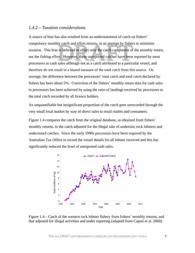
Figure 1.4 compares the catch from the original database, as obtained from fishers’
monthly returns, to the catch adjusted for the illegal take of undersize rock lobsters and
understated catches. Since the early 1990s processors have been required by the
Australian Tax Office to record the vessel details for all lobster received and this has
significantly reduced the level of unreported cash sales.
0
2
4
6
8
10
12
14
16
1940 1950 1960 1970 1980 1990 2000 2010
Year
Cat
ch (m
illio
ns o
f kg)
Catch Adjusted Catch
Figure 1.4 – Catch of the western rock lobster fishery from fishers’ monthly returns, and that adjusted for illegal activities and under reporting (adapted from Caputi et al. 2000).
This is a DRAFT and information is solely for pre-dissemination peer review 7
2 – Management
DRAFTManagement regulations are aimed primary at protection of the breeding stock with
regulations continually reviewed, to ensure the breeding stock is maintained at a
sustainable level, i.e. above a threshold Biological Reference Point (BRP). DRAFT
2.1 – Management Objective
The threshold BRP for a sustainable breeding stock was deemed to be the egg production
in 1980. Egg production in the late 1970s and early 1980s was estimated, using a length-
based assessment model, to be around 20% of the unfished level (Hall and Chubb 2001).
This level was considered appropriate in the sustainability of many other invertebrate
fisheries (Hall & Chubb 2001). Biologically, management measures are designed to;
“Ensure the abundance of breeding lobsters is maintained or returned to, as the case
may be, at or above the levels in 1980.” (from Department of Fisheries 2005)
This is a DRAFT and information is solely for pre-dissemination peer review 8
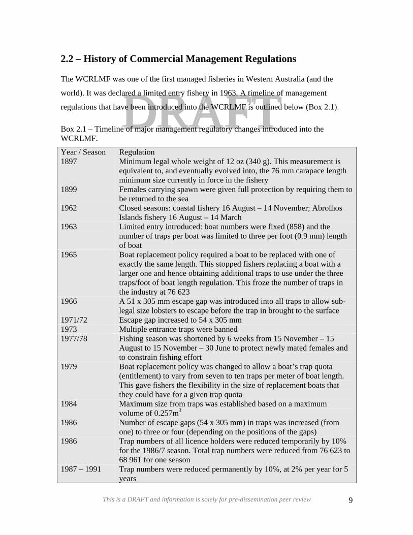
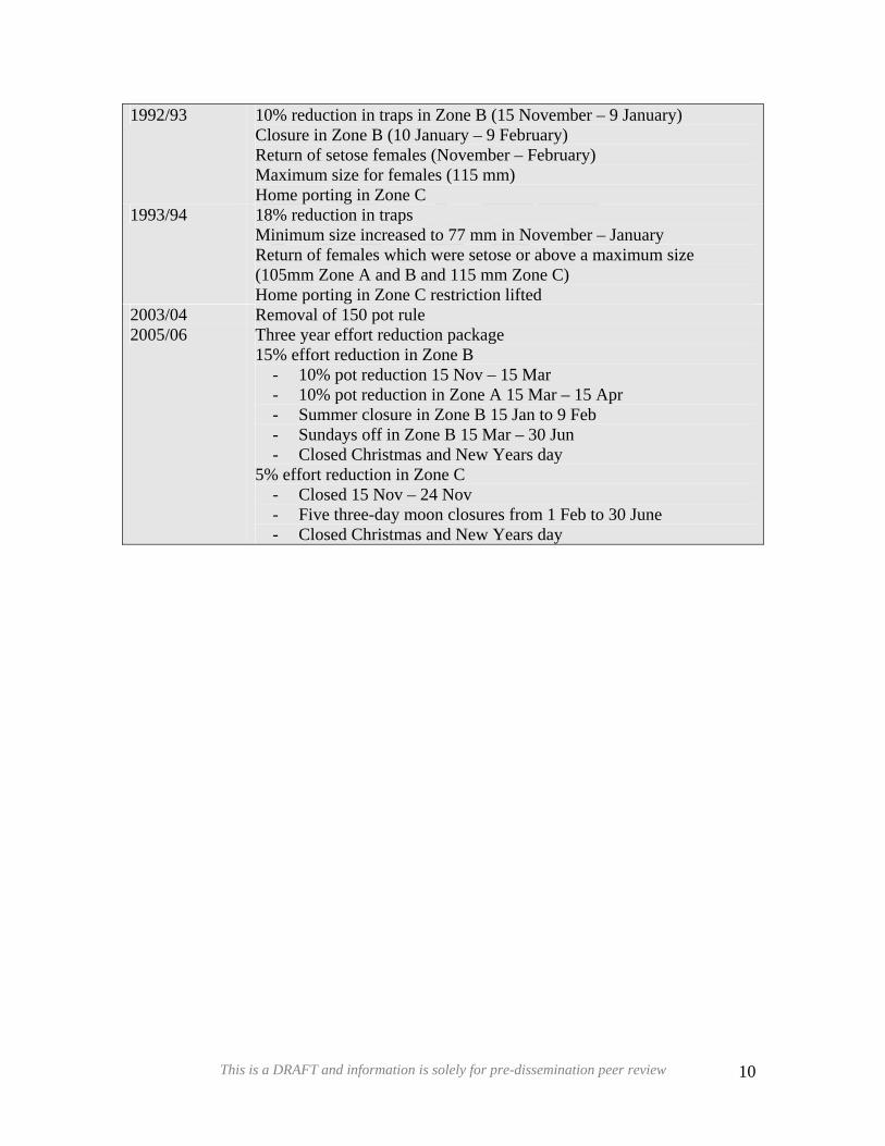
2.2 – History of Commercial Management Regulations
DDRRAAFFTTThe WCRLMF was one of the first managed fisheries in Western Australia (and the
world). It was declared a limited entry fishery in 1963. A timeline of management
regulations that have been introduced into the WCRLMF is outlined below (Box 2.1).
Box 2.1 – Timeline of major management regulatory changes introduced into the WCRLMF.
Year / Season Regulation 1897 Minimum legal whole weight of 12 oz (340 g). This measurement is
equivalent to, and eventually evolved into, the 76 mm carapace length minimum size currently in force in the fishery
1899 Females carrying spawn were given full protection by requiring them to be returned to the sea
1962 Closed seasons: coastal fishery 16 August – 14 November; Abrolhos Islands fishery 16 August – 14 March
1963 Limited entry introduced: boat numbers were fixed (858) and the number of traps per boat was limited to three per foot (0.9 mm) length of boat
1965 Boat replacement policy required a boat to be replaced with one of exactly the same length. This stopped fishers replacing a boat with a larger one and hence obtaining additional traps to use under the three traps/foot of boat length regulation. This froze the number of traps in the industry at 76 623
1966 A 51 x 305 mm escape gap was introduced into all traps to allow sub-legal size lobsters to escape before the trap in brought to the surface
1971/72 Escape gap increased to 54 x 305 mm 1973 Multiple entrance traps were banned 1977/78 Fishing season was shortened by 6 weeks from 15 November – 15
August to 15 November – 30 June to protect newly mated females and to constrain fishing effort
1979 Boat replacement policy was changed to allow a boat’s trap quota (entitlement) to vary from seven to ten traps per meter of boat length. This gave fishers the flexibility in the size of replacement boats that they could have for a given trap quota
1984 Maximum size from traps was established based on a maximum volume of 0.257m3
1986 Number of escape gaps (54 x 305 mm) in traps was increased (from one) to three or four (depending on the positions of the gaps)
1986 Trap numbers of all licence holders were reduced temporarily by 10% for the 1986/7 season. Total trap numbers were reduced from 76 623 to 68 961 for one season
1987 – 1991 Trap numbers were reduced permanently by 10%, at 2% per year for 5 years
This is a DRAFT and information is solely for pre-dissemination peer review 9
DDRRAAFFTT1992/93 10% reduction in traps in Zone B (15 November – 9 January)
Closure in Zone B (10 January – 9 February) Return of setose females (November – February) Maximum size for females (115 mm) Home porting in Zone C
1993/94 18% reduction in traps Minimum size increased to 77 mm in November – January Return of females which were setose or above a maximum size (105mm Zone A and B and 115 mm Zone C) Home porting in Zone C restriction lifted
2003/04 Removal of 150 pot rule 2005/06 Three year effort reduction package
15% effort reduction in Zone B - 10% pot reduction 15 Nov – 15 Mar - 10% pot reduction in Zone A 15 Mar – 15 Apr - Summer closure in Zone B 15 Jan to 9 Feb - Sundays off in Zone B 15 Mar – 30 Jun - Closed Christmas and New Years day
5% effort reduction in Zone C - Closed 15 Nov – 24 Nov - Five three-day moon closures from 1 Feb to 30 June - Closed Christmas and New Years day
This is a DRAFT and information is solely for pre-dissemination peer review 10
2.3 – Boundaries and Zoning
DDRRAAFFTT‘the waters situated on the west coast of the State bounded by a line commencing at the
intersection of the high water mark and 21°44´ south latitude drawn due west to the
intersection of 21°44´ south latitude and the boundary of the Australian Fishing Zone;
thence southwards along the boundary to its intersection with 34°24´ south latitude;
thence due east along 34°24´ south latitude to the intersection of 115°08´ east longitude;
thence due north along 115°08´ east longitude to the high water mark; thence along the
high water mark to the commencing point and divided into zones’.
The boundaries of the WCRLMF are:
The fishery is managed in three zones: south of latitude 30° S (Zone C), north of latitude
30° S (Zone B) and, within this northern area, a third offshore zone (Zone A) around the
Abrolhos Islands (Figure 2.1). This distributes effort across the entire fishery, and allows
for the implementation of management controls aimed at addressing zone-specific issues,
including different maximum size restrictions in the northern and southern regions of the
fishery. The season is open from 15th November to 30th June annually; with the Abrolhos
Islands zone operating from 15th March to 30th June.
This is a DRAFT and information is solely for pre-dissemination peer review 11
DDRRAAFFTT
Figure 2.1 – Western Rock Lobster Fishery Management Zones
This is a DRAFT and information is solely for pre-dissemination peer review 12
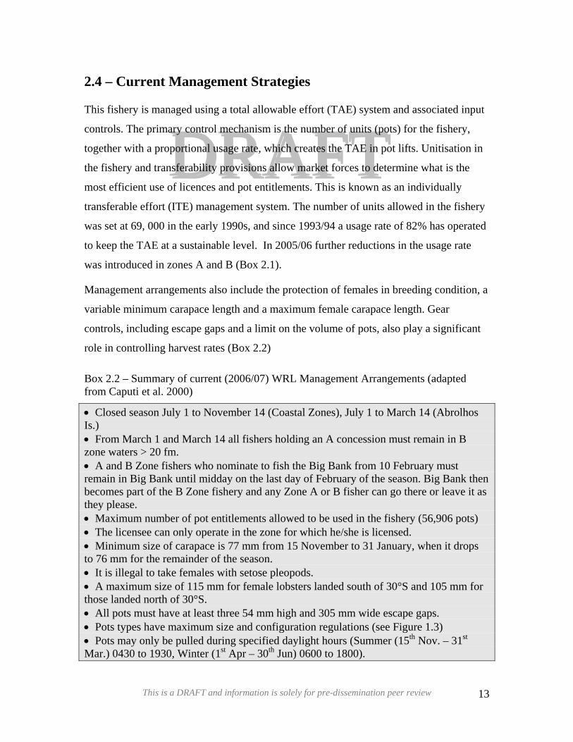
2.4 – Current Management Strategies
DDRRAAFFTTThis fishery is managed using a total allowable effort (TAE) system and associated input
controls. The primary control mechanism is the number of units (pots) for the fishery,
together with a proportional usage rate, which creates the TAE in pot lifts. Unitisation in
the fishery and transferability provisions allow market forces to determine what is the
most efficient use of licences and pot entitlements. This is known as an individually
transferable effort (ITE) management system. The number of units allowed in the fishery
was set at 69, 000 in the early 1990s, and since 1993/94 a usage rate of 82% has operated
to keep the TAE at a sustainable level. In 2005/06 further reductions in the usage rate
was introduced in zones A and B (Box 2.1).
Management arrangements also include the protection of females in breeding condition, a
variable minimum carapace length and a maximum female carapace length. Gear
controls, including escape gaps and a limit on the volume of pots, also play a significant
role in controlling harvest rates (Box 2.2)
Box 2.2 – Summary of current (2006/07) WRL Management Arrangements (adapted from Caputi et al. 2000)
• Closed season July 1 to November 14 (Coastal Zones), July 1 to March 14 (Abrolhos Is.) • From March 1 and March 14 all fishers holding an A concession must remain in B zone waters > 20 fm. • A and B Zone fishers who nominate to fish the Big Bank from 10 February must remain in Big Bank until midday on the last day of February of the season. Big Bank then becomes part of the B Zone fishery and any Zone A or B fisher can go there or leave it as they please. • Maximum number of pot entitlements allowed to be used in the fishery (56,906 pots) • The licensee can only operate in the zone for which he/she is licensed. • Minimum size of carapace is 77 mm from 15 November to 31 January, when it drops to 76 mm for the remainder of the season. • It is illegal to take females with setose pleopods. • A maximum size of 115 mm for female lobsters landed south of 30°S and 105 mm for those landed north of 30°S. • All pots must have at least three 54 mm high and 305 mm wide escape gaps. • Pots types have maximum size and configuration regulations (see Figure 1.3) • Pots may only be pulled during specified daylight hours (Summer (15th Nov. – 31st Mar.) 0430 to 1930, Winter (1st Apr – 30th Jun) 0600 to 1800).
This is a DRAFT and information is solely for pre-dissemination peer review 13
• To operate in the managed fishery, a licence must have at least 63 units of pot entitlement.
DDRRAAFFTT• Three-year effort reduction package (Box 2.1 – 2005/6)
2.4.1 Recreational Specific Management Strategies
The recreational component of the western rock lobster fishery is managed under
fisheries regulations that impose a mix of input and output controls on individual
recreational fishers. These arrangements are designed to complement the management
plan for the commercial fishery.
Input controls include the requirement for a recreational fishing licence (either a specific
rock lobster licence or an ‘umbrella’ licence covering all licensed recreational fisheries).
Fishers are restricted to two pots per licence holder, although the total number of licences
is not restricted. The pots must meet the specific size requirements, smaller than those for
the commercial fishers, and must have gaps to allow under-size rock lobsters to escape
(see web site
http://www.fish.wa.gov.au/docs/pub/FishingRockLobsters/FishingforRockLobstersPage0
6.php?0102 for specific details on recreational pot dimensions). Divers are also restricted
to catching by hand, snare or blunt crook in order that lobsters are not damaged. Fishing
for rock lobsters at the Abrolhos Islands is restricted to potting only.
The recreational fishing season runs from 15th November to 30th June each year, with a
shorter season (15th March to 30th June) at the Abrolhos Islands. Night-time fishing for
lobsters by diving prohibited.
Recreational fishers comply with the same legislation as the commercial fishers with
regard to the size and condition of lobsters they can take and when, except there is a daily
bag limit of 8 lobsters per fisher per day. A daily boat limit of 16 lobsters provides further
control on high individual catches where there are three or more people fishing from the
same boat. In the Ningaloo Marine Park and between Cape Preston and Cape Lambert in
the Dampier Archipelago, the daily bag limit is 4 and the boat limit 8 lobsters. There is
also a requirement for recreationally caught lobsters to be tail-clipped in order to stop
these animals from being sold illegally.
This is a DRAFT and information is solely for pre-dissemination peer review 14

2.5 – Marine Stewardship Council (MSC) Certification
DDRRAAFFTTIn 2000, the West Coast Rock Lobster Managed Fishery became the world’s first fishery
to receive Marine Stewardship Council (MSC) certification on the basis of demonstrating
the sustainability of its fishing and management operations. To achieve this, the WRL
fishery was assessed by an international group of experts against the criteria set out in the
MSC guidelines (see web site http://www.msc.org/ for details). A number of ongoing
requirements have had to be met to continue this accreditation including an ecological
risk assessment and the development and implementation of an Environmental
Management Strategy (EMS). Ecological Risk Assessment (ERA) workshops have been
conducted to provide a register of the potential ecological risks arising from the various
activities carried out by the WCRLMF. The fishery was recertified in December 2006.
This is a DRAFT and information is solely for pre-dissemination peer review 15
2.6 – Integrated Fisheries Management (IFM)
DDRRAAFFTTIntegrated Fisheries Management (IFM) is the most recent management development in
Western Australia fisheries and is designed to ensure that all sectors are taken into
account in the management of the states fisheries. A core objective is to determine how to
share the available fishery resource between competing users, while maintaining the
fishery stock at an ecologically sustainable level. As such it requires;
o Setting an ecologically Sustainable Harvest Level (SHL) for the whole fishery
o Allocating a share of the SLH between indigenous, commercial and recreational
users.
o Monitoring of each sectors catch.
o Managing each sector so as to remain within its respective catch allocation.
o Developing processes which enable re-allocation of catch shares between sectors.
The West Coast Rock Lobster Fishery was the first fishery in the state to go through the
IFM process. Currently the IFM process for the WCRLMF has resulted in an allocation
report (IFAAC 2007). In this, the Minister’s proposed position is that the recreational and
commercial allocations should be five per cent and 95 per cent respectively, and that
there should be a customary fishing initial allocation of one tonne. The Minister has
proposed that the allocations be implemented in 2009/10. Opportunity for submissions to
these proposals closed on 23rd April 2007. Notification of final decisions has yet to be
made (IFAAC 2007).
This is a DRAFT and information is solely for pre-dissemination peer review 16
3 – Biology
DDRRAAFFTT3.1 – Taxonomy
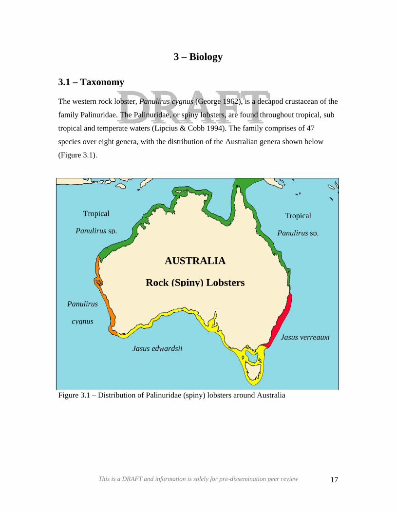
The western rock lobster, Panulirus cygnus (George 1962), is a decapod crustacean of the
family Palinuridae. The Palinuridae, or spiny lobsters, are found throughout tropical, sub
tropical and temperate waters (Lipcius & Cobb 1994). The family comprises of 47
species over eight genera, with the distribution of the Australian genera shown below
(Figure 3.1).
Tropical
Panulirus sp.
Panulirus
cygnus
Jasus edwardsii Jasus verreauxi
Tropical
Panulirus sp.
AUSTRALIA
Rock (Spiny) Lobsters
Figure 3.1 – Distribution of Palinuridae (spiny) lobsters around Australia
This is a DRAFT and information is solely for pre-dissemination peer review 17
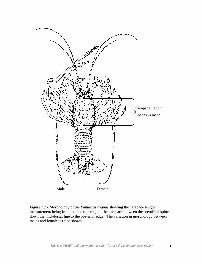
DDRRAAFFTT
Carapace Length
Measurement
Male Female
Figure 3.2 - Morphology of the Panulirus cygnus showing the carapace length measurement being from the anterior edge of the carapace between the preorbital spines down the mid-dorsal line to the posterior edge. The variation in morphology between males and females is also shown.
This is a DRAFT and information is solely for pre-dissemination peer review 18
3.2 – Stock Structure
DDRRAAFFTTSamples of legal-sized lobster from 1980 (Thompson et al. 1996), and puerulus from
1995 to 1998 (Johnson 1999), showed some latitudinal and temporal variation in allelic
frequencies in polymorphic loci. However the 1994 sample of Thompson et al. (1996)
showed that this latitudinal variation was not persistent through years.
The stock structure of WRL has been examined genetically through allozyme
electrophoresis (Thompson et al. 1996, Johnson 1999).
The overarching conclusion from both studies is that the western rock lobster is a single
panmictic population, with ephemeral genetic patchiness between cohorts (Thompson et
al. 1996, Johnson 1999).
However, there is variation in reproductive biology (Section 3.6) and growth (Section
3.8). At this stage there is uncertainty as to whether these observed changes in life history
parameters are the result of changes in environmental conditions, a response to selective
fishing practices or a combination of possibilities (Melville-Smith & de Lestang 2006).
However, they do necessitate the assessment and management of the fishery in zones, so
as to account for this biological variation and tailor management accordingly (Section 2).
This is a DRAFT and information is solely for pre-dissemination peer review 19
3.3 – Habitats
DRAFTThe distributional range of P. cygnus (Figure 1.1) sees it restricted to the clear, warm, low
nutrient waters of the west coast of Western Australia. These oceanic conditions are
markedly different from those on the eastern edge of other ocean systems like the
Atlantic and Pacific in the southern hemisphere. These coasts have cold, northward
flowing currents (Humbolt and Benguela currents) producing nutrient rich up-wellings
near the coast. In contrast the eastern coast of the Indian Ocean is dominated by a
southward flowing, warm tropical water of the Leeuwin Current (Plate 3.1).
DRAFT3.2.1 – Oceanography
The Leeuwin Current is strongest during the southern autumn and winter (March to
October) when it flows from the northwest of Australia, along the coast and around into
the Great Australian Bight. Between North West Cape and Shark Bay it approaches the
coast where it has a broad shallow flow, before narrowing and deepening to about 150 –
200 m and 30 km wide along the continental shelf. As it nears Cape Leeuwin it moves up
onto the continental shelf and flows into the Great Australian Bight. As the current skirts
the coastline it forms gyres or eddies; offshoots of the main current. These are highly
variable in terms of their duration (days to months), size (some may be over a 100 km in
diameter), and are usually consistent in their location (Plate 3.1).
This is a DRAFT and information is solely for pre-dissemination peer review 20
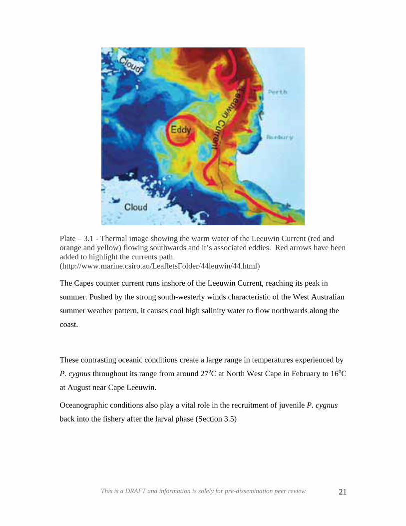
DDRRAAFFTT
Plate – 3.1 - Thermal image showing the warm water of the Leeuwin Current (red and orange and yellow) flowing southwards and it’s associated eddies. Red arrows have been added to highlight the currents path (http://www.marine.csiro.au/LeafletsFolder/44leuwin/44.html)
The Capes counter current runs inshore of the Leeuwin Current, reaching its peak in
summer. Pushed by the strong south-westerly winds characteristic of the West Australian
summer weather pattern, it causes cool high salinity water to flow northwards along the
coast.
These contrasting oceanic conditions create a large range in temperatures experienced by
P. cygnus throughout its range from around 27oC at North West Cape in February to 16oC
at August near Cape Leeuwin.
Oceanographic conditions also play a vital role in the recruitment of juvenile P. cygnus
back into the fishery after the larval phase (Section 3.5)
This is a DRAFT and information is solely for pre-dissemination peer review 21

3.2.2 – Physical Habitat
DRAFTDRAFTThe distribution of P. cygnus is dominated by limestone reefs, which can extend seaward
for 40 to 60 km on the continental shelf. This habitat is the almost exclusive domain of P.
cygnus with minimal overlap of other rock lobster species (Figure 3.1).
Changes in sea levels have caused the fringing reefs associated with lower sea level
shorelines to be submerged, forming long chains of ledges and banks. Also, sea level
changes have created a number of mainland remnant islands with associated fringing
reefs. These reefs and banks often contain a matrix of crevices and ledges, which are the
primary diurnal habitat of P. cygnus.
Water depth, light and wave exposure influence the flora and fauna on these limestone
reefs and banks. The reefs are typically covered by seagrass (Amphibolis), and large
algae. At greater depths, and up to 50 m, large brown algae (Ecklonia and Sargassum)
create “kelp” gardens covering the hard limestone bottom, while crevices, where light
penetration is reduced, is often covered with seasquirts, sponges and other sessile
invertebrates.
The influence of the Leeuwin Current also creates a range of habitats within the
distribution of P. cygnus. While the limestone reefs and pavements dominate, there are
some coral reefs, particularly at the Houtman Abrolhos Islands, which are important rock
lobster habitats.
This is a DRAFT and information is solely for pre-dissemination peer review 22
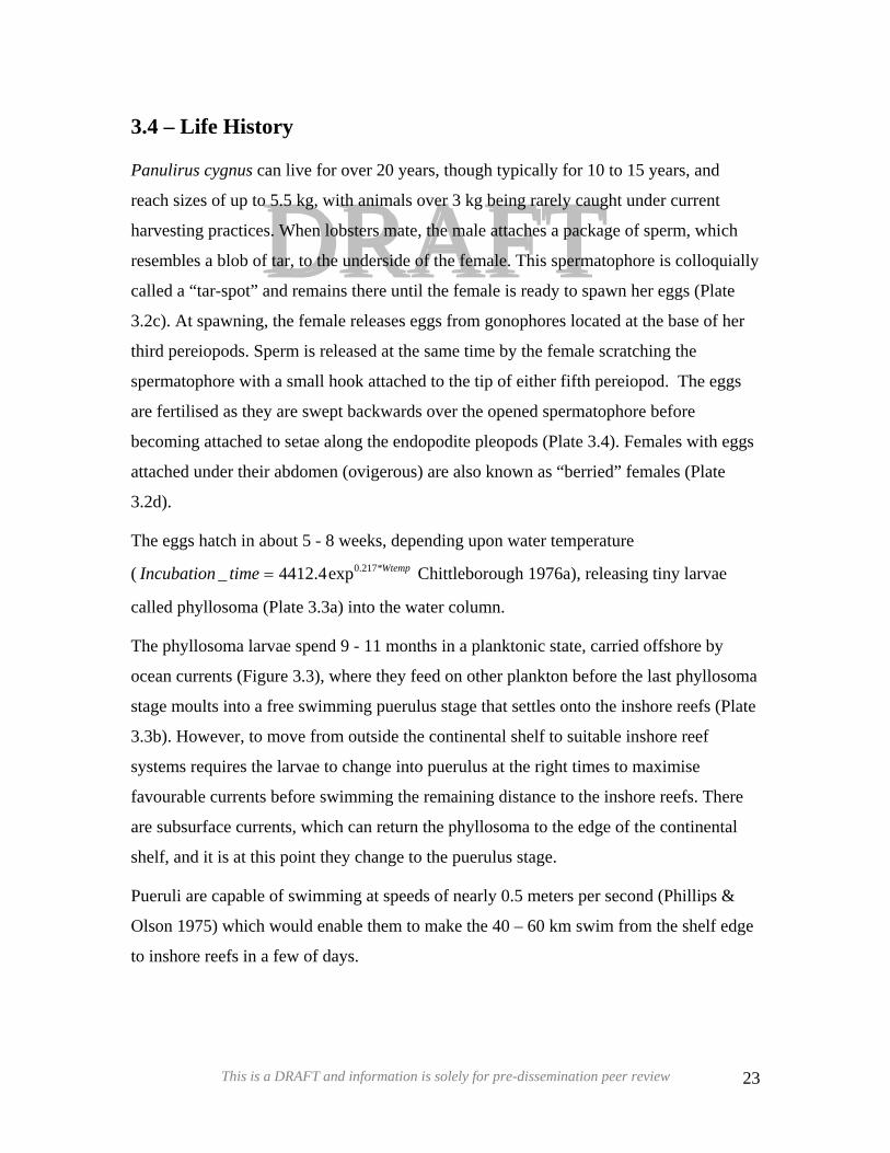
3.4 – Life History
DDRRAAFFTTPanulirus cygnus can live for over 20 years, though typically for 10 to 15 years, and
reach sizes of up to 5.5 kg, with animals over 3 kg being rarely caught under current
harvesting practices. When lobsters mate, the male attaches a package of sperm, which
resembles a blob of tar, to the underside of the female. This spermatophore is colloquially
called a “tar-spot” and remains there until the female is ready to spawn her eggs (Plate
3.2c). At spawning, the female releases eggs from gonophores located at the base of her
third pereiopods. Sperm is released at the same time by the female scratching the
spermatophore with a small hook attached to the tip of either fifth pereiopod. The eggs
are fertilised as they are swept backwards over the opened spermatophore before
becoming attached to setae along the endopodite pleopods (Plate 3.4). Females with eggs
attached under their abdomen (ovigerous) are also known as “berried” females (Plate
3.2d).
The eggs hatch in about 5 - 8 weeks, depending upon water temperature
( Chittleborough 1976a), releasing tiny larvae
called phyllosoma (Plate 3.3a) into the water column.
WtemptimeIncubation *217.0exp4.4412_ =
The phyllosoma larvae spend 9 - 11 months in a planktonic state, carried offshore by
ocean currents (Figure 3.3), where they feed on other plankton before the last phyllosoma
stage moults into a free swimming puerulus stage that settles onto the inshore reefs (Plate
3.3b). However, to move from outside the continental shelf to suitable inshore reef
systems requires the larvae to change into puerulus at the right times to maximise
favourable currents before swimming the remaining distance to the inshore reefs. There
are subsurface currents, which can return the phyllosoma to the edge of the continental
shelf, and it is at this point they change to the puerulus stage.
Pueruli are capable of swimming at speeds of nearly 0.5 meters per second (Phillips &
Olson 1975) which would enable them to make the 40 – 60 km swim from the shelf edge
to inshore reefs in a few of days.
This is a DRAFT and information is solely for pre-dissemination peer review 23
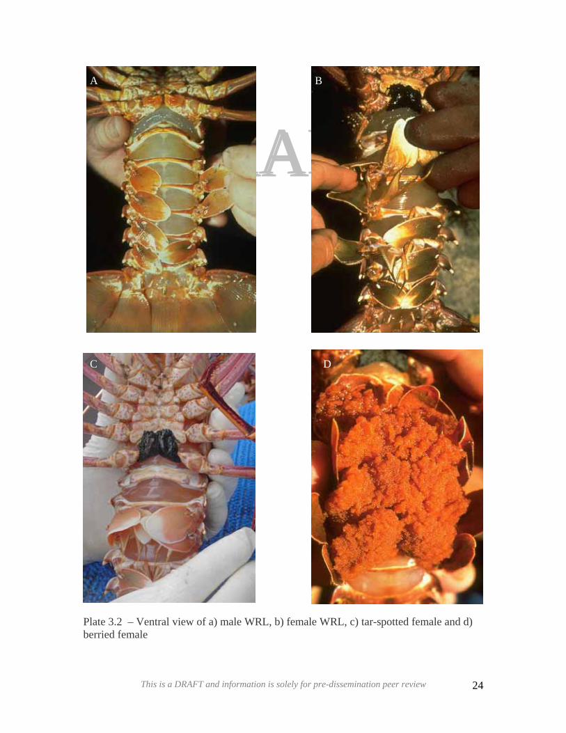
Pb
A
DDRRAAFF
late 3.2 – Ventral view of a) male WRL, b) femalerried female
This is a DRAFT and information is solely for
B
TT
C
e
pr
D
WRL, c) tar-spotted female and d)
e-dissemination peer review 24
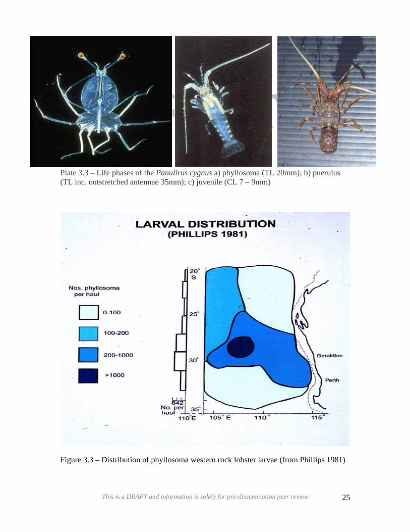
DDRRAAFFTTPlate 3.3 – Life phases of the Panulirus cygnus a) phyllosoma (TL 20mm); b) puerulus (TL inc. outstretched antennae 35mm); c) juvenile (CL 7 – 9mm)
Figure 3.3 – Distribution of phyllosoma western rock lobster larvae (from Phillips 1981)
This is a DRAFT and information is solely for pre-dissemination peer review 25
DDRRAAFFTTPueruli that successfully return to the coast, move close inshore, presumably in
association with sea grass beds and algal meadows, before they moult into a juvenile
phase (Plate 3.3c). For details of pueruli recruitment to inshore areas, see Section 3.5.
Phillips and MacMillan (1987) theorised that detection of the coast by puerulus was done
by using their antennae acting as vibration receptors, detecting ocean swell noise on the
coasts or offshore reefs.
These juveniles feed and grow on the shallow inshore reefs for the next three or four
years by which time they can achieve CLs up to 80mm. Three to four years after
settlement, many lobsters undergo a synchronised moult in late spring when they moult
from their normal red shell colour into a paler colour. These are known as “white”
lobsters until they return to their normal red colour at the next moult a few months later.
The “white” phase of a rock lobster’s life is the migratory phase (Section 3.5.1). At this
time (summer) they leave the coastal reefs and undergo a mass migration across pale
white sands into deeper water breeding grounds where they become sedentary again on
deeper reefs. A small percentage make far longer migrations off the edge of the
continental shelf down to depths of over 200 m, before they change direction and follow
the shelf in a northerly direction. Once reaching the offshore breeding grounds the
“whites” undergo another synchronised moult at which time their exoskeleton becomes
reds in colour (February – March). This deeper offshore ground is where the spawning
stock predominantly resides (Figure 3.4).
This is a DRAFT and information is solely for pre-dissemination peer review 26
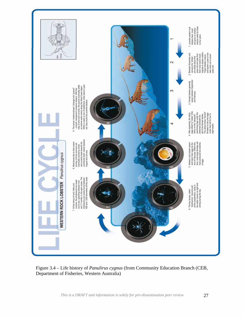
DDRRAAFFTT
Figure 3.4 – Life history of Panulirus cygnus (from Community Education Branch (CEB, Department of Fisheries, Western Australia)
This is a DRAFT and information is solely for pre-dissemination peer review 27
3.5 – Movement
DDRRAAFFTTMovement patterns of P. cygnus have been and continue to be studied extensively.
Research has primarily focused on two aspects of the lobster’s movement; namely, the
“whites” migration and small-scale foraging movements.
3.5.1 – Migration
The large-scale “whites” migration is a feature of this lobster’s life history (Section 3.4).
Tagging studies (using mainly external “T-bar” anchor tags) have been undertaken to
assess this aspect of the lobster’s life history (Melville-Smith et al. 1998, Chubb et al.
1999) as well as to provide growth information (Section 3.8).
Chubb et al. (1999) tagged and released over 66 500 lobster between 1988 and 1996
throughout the fishery. Approximately 75% of the recaptures were during the first season
after release with around 20% the following season, though recaptures did occur up to 5
seasons after release.
While large movements (>200 km) did occur, most movements were usually west or
north-westerly in direction and less than 50 km, with the vast majority (87 – 98% by
location) being recaptured within 10 km of their release site.
It was found that “whites” moved considerably further than the “reds”. This was also
evident when movement was examined with regard to size, with those between 70 – 90
mm CL moving further. “White” movements greater than 10 km accounted for 27% of
the movements, while for the “reds” they were only 9%. This is thought to be an
underestimate for whites and overestimate of red movements, due to lobster being tagged
and recaptured as “reds”, despite their size during time at liberty indicating that they
probably passed through a “whites” moult. This assumption could not be tested and
therefore, neither could the suspected cause for the under or overestimation of movement
be confirmed.
The timing of migration, and potential cues for it, are currently being investigated.
Factors that appear to be related to lobster migration include average water temp for the
7-day period immediately before the start of migration include, the moon illumination
This is a DRAFT and information is solely for pre-dissemination peer review 28
DDRRAAFFTTTo this stage the lobster migration prediction model has been hampered by the lack of
water temperature data at 1
and total sea swell levels at the start of migration. To date the best single predictor of
migration has been found to be moon illumination (migration taking place close to a new
or full moon). After this water temperature seemed to add further power for predicting the
start of migration (warmer water temperature encouraged migration).
o intervals (at the moment we are using one temperature
measure for each zone but estimating ‘start of migration’ times at 1o levels, using logbook
data) to better explain the migration of animals at this level.
3.5.2 – Foraging
Small-scale foraging movement patterns of juvenile P. cygnus have been studied using
tag recapture (Chittleborough 1974a), or electromagnetic tracking (Jernakoff 1987,
Jernakoff et al. 1987, Jernakoff & Phillips 1988).
Jernakoff & Phillips (1988) estimated foraging distances of ~150 m radius from dens.
Jernakoff et al. (1987) also showed movements to be very variable, with distance of
between 72.5 and 585 m accounting for 95% of all foraging distances in the study. One
individual moved 803 m in a night within the tracking area.
These results demonstrate that juvenile P. cygnus forage over relatively small areas,
though the extent of movement is variable.
More recently, technology has advanced allowing automated tracking of juveniles
through acoustic tags (MacArthur unpublished data) and adults in deeper environment
(Section 7.1.2). To date, this data has not been analysed, but will provide information on
foraging distances, home ranges and habitat use of adult and juvenile P. cygnus.
This is a DRAFT and information is solely for pre-dissemination peer review 29
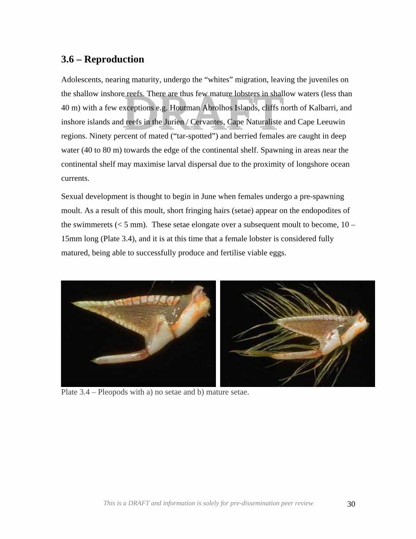
3.6 – Reproduction
DDRRAAFFTTAdolescents, nearing maturity, undergo the “whites” migration, leaving the juveniles on
the shallow inshore reefs. There are thus few mature lobsters in shallow waters (less than
40 m) with a few exceptions e.g. Houtman Abrolhos Islands, cliffs north of Kalbarri, and
inshore islands and reefs in the Jurien / Cervantes, Cape Naturaliste and Cape Leeuwin
regions. Ninety percent of mated (“tar-spotted”) and berried females are caught in deep
water (40 to 80 m) towards the edge of the continental shelf. Spawning in areas near the
continental shelf may maximise larval dispersal due to the proximity of longshore ocean
currents.
Sexual development is thought to begin in June when females undergo a pre-spawning
moult. As a result of this moult, short fringing hairs (setae) appear on the endopodites of
the swimmerets (< 5 mm). These setae elongate over a subsequent moult to become, 10 –
15mm long (Plate 3.4), and it is at this time that a female lobster is considered fully
matured, being able to successfully produce and fertilise viable eggs.
P
Alate 3.4 – Pleopods with a) no setae and b) matu
This is a DRAFT and information is solely f
B
re setae.
or pre-dissemination peer review 30
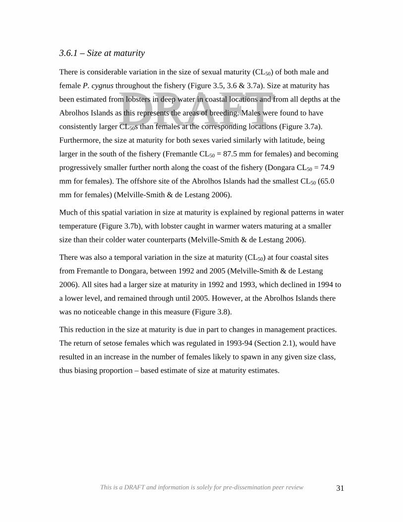
3.6.1 – Size at maturity
DRAFTThere is considerable variation in the size of sexual maturity (CL
DRAFT50) of both male and
female P. cygnus throughout the fishery (Figure 3.5, 3.6 & 3.7a). Size at maturity has
been estimated from lobsters in deep water in coastal locations and from all depths at the
Abrolhos Islands as this represents the areas of breeding. Males were found to have
consistently larger CL50s than females at the corresponding locations (Figure 3.7a).
Furthermore, the size at maturity for both sexes varied similarly with latitude, being
larger in the south of the fishery (Fremantle CL50 = 87.5 mm for females) and becoming
progressively smaller further north along the coast of the fishery (Dongara CL50 = 74.9
mm for females). The offshore site of the Abrolhos Islands had the smallest CL50 (65.0
mm for females) (Melville-Smith & de Lestang 2006).
Much of this spatial variation in size at maturity is explained by regional patterns in water
temperature (Figure 3.7b), with lobster caught in warmer waters maturing at a smaller
size than their colder water counterparts (Melville-Smith & de Lestang 2006).
There was also a temporal variation in the size at maturity (CL50) at four coastal sites
from Fremantle to Dongara, between 1992 and 2005 (Melville-Smith & de Lestang
2006). All sites had a larger size at maturity in 1992 and 1993, which declined in 1994 to
a lower level, and remained through until 2005. However, at the Abrolhos Islands there
was no noticeable change in this measure (Figure 3.8).
This reduction in the size at maturity is due in part to changes in management practices.
The return of setose females which was regulated in 1993-94 (Section 2.1), would have
resulted in an increase in the number of females likely to spawn in any given size class,
thus biasing proportion – based estimate of size at maturity estimates.
This is a DRAFT and information is solely for pre-dissemination peer review 31
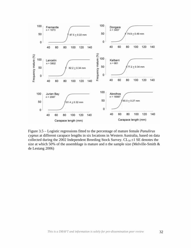
DDRRAAFFTT
Figure 3.5 – Logistic regressions fitted to the percentage of mature female Panulirus cygnus at different carapace lengths in six locations in Western Australia, based on data collected during the 2002 Independent Breeding Stock Survey. CL50 ±1 SE denotes the size at which 50% of the assemblage is mature and n the sample size (Melville-Smith & de Lestang 2006)
This is a DRAFT and information is solely for pre-dissemination peer review 32
DDRRAAFFTT
Figure 3.6 – Relationship between the merus length of the second pereiopod and carapace length of immature (open circle) and mature (filled circle) male Panulirus cygnus (left) and logistic regressions fitted to the percentage of morphometrically mature males at different carapace lengths (right) in six locations in Western Australia, based on data collected during the 2002 Independent Breeding Stock Survey. CL50±1 SE denotes the size at which 50% of the assemblage is mature and n the sample size (Melville-Smith & de Lestang 2006).
This is a DRAFT and information is solely for pre-dissemination peer review 33
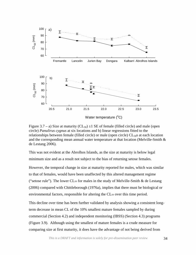
CL 50
(mm
)
60
70
80
90
100
)C
L 50 (m
m)
60
70
80
90
100
Figure 3.7 –circle) Panurelationshipand the corrde Lestang 2
This was no
minimum si
However, th
to that of fem
(“setose rule
(2006) comp
environmen
This decline
term decrea
commercial
(Figure 3.9)
comparing s
aa)
DDRRAAFFTT
Water temperature (oC)
20.5 21.0 21.5 22.0 22.5 23.0 23.5
b)
Fremantle Lancelin Jurien Bay Dongara Kalbarri Abrolhos Islands
a) Size at maturity (CL50) ±1 SE of female (filled circle) and male (open lirus cygnus at six locations and b) linear regressions fitted to the s between female (filled circle) or male (open circle) CL50s at each location esponding mean annual water temperature at that location (Melville-Smith & 006).
t evident at the Abrolhos Islands, as the size at maturity is below legal
ze and as a result not subject to the bias of returning setose females.
e temporal change in size at maturity reported for males, which was similar
ales, would have been unaffected by this altered management regime
”). The lower CL50 for males in the study of Melville-Smith & de Lestang
ared with Chittleborough (1976a), implies that there must be biological or
tal factors, responsible for altering the CL50 over this time period.
over time has been further validated by analysis showing a consistent long-
se in mean CL of the 10% smallest mature females sampled by during
(Section 4.2) and independent monitoring (IBSS) (Section 4.3) programs
. Although using the smallest of mature females is a crude measure for
ize at first maturity, it does have the advantage of not being derived from
This is a DRAFT and information is solely for pre-dissemination peer review 34
DDRRAAFFTTratios of immature and mature animals and as such, not being influenced by the “setose
rule”. The mean CLs of the 10% smallest females sampled during commercial monitoring
were, in the majority of cases, larger than corresponding values determined from IBSS
data. This difference is due mainly to the IBSS being conducted over the peak of the
breeding season (October to November) at the point when the majority of all mature
females are mated or egg bearing. The commercial monitoring on the other hand does
not begin until after the IBSS and covers the subsequent decline in breeding activity
when small single breeding females are no longer reproductively active and can even
have moulted into their non-reproductive phase, while large double-breeding females can
still be brooding eggs (de Lestang and Melville-Smith, in press). In fact, even though the
IBSS is conducted over the same new moon period prior to the start of the fishing season
(15th November), it does not always align with the peak of the breeding season. This
variation between the timing of the IBSS and that of peak spawning is one factor
contributing to the oscillating CL50 estimates for the various sites each year since 1994
(Figure 3.9).
This is a DRAFT and information is solely for pre-dissemination peer review 35
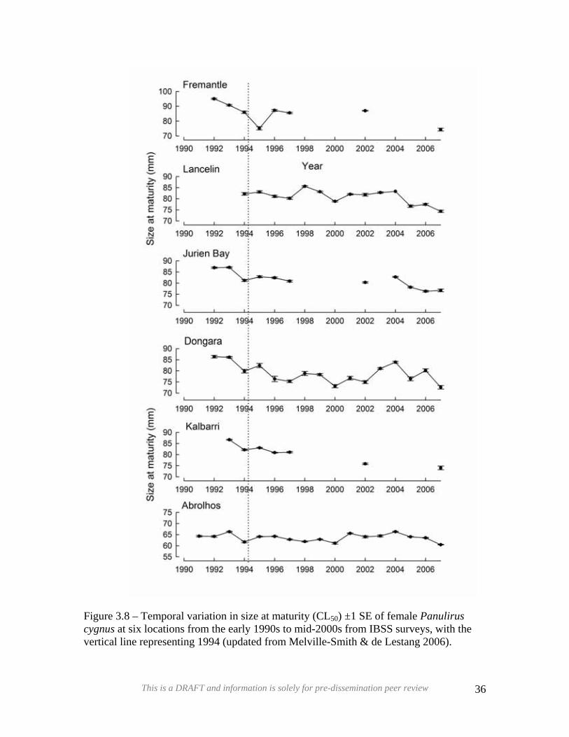
DDRRAAFFTT
Figure 3.8 – Temporal variation in size at maturity (CL50) ±1 SE of female Panulirus cygnus at six locations from the early 1990s to mid-2000s from IBSS surveys, with the vertical line representing 1994 (updated from Melville-Smith & de Lestang 2006).
This is a DRAFT and information is solely for pre-dissemination peer review 36
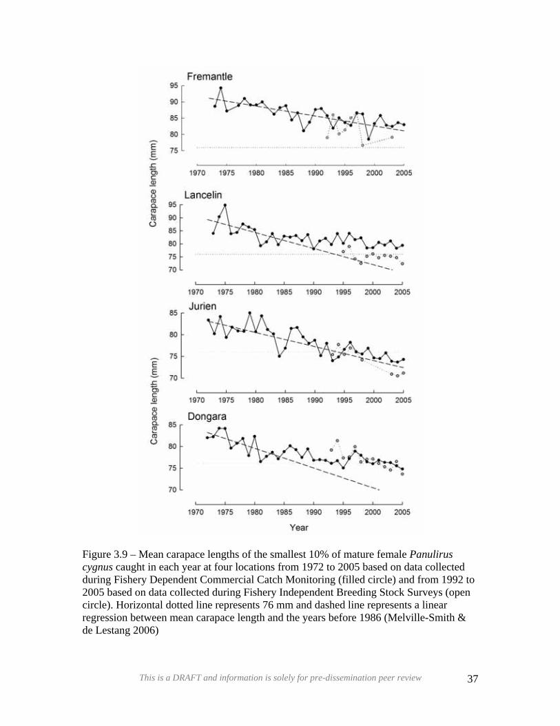
DDRRAAFFTT
Figure 3.9 – Mean carapace lengths of the smallest 10% of mature female Panulirus cygnus caught in each year at four locations from 1972 to 2005 based on data collected during Fishery Dependent Commercial Catch Monitoring (filled circle) and from 1992 to 2005 based on data collected during Fishery Independent Breeding Stock Surveys (open circle). Horizontal dotted line represents 76 mm and dashed line represents a linear regression between mean carapace length and the years before 1986 (Melville-Smith & de Lestang 2006)
This is a DRAFT and information is solely for pre-dissemination peer review 37
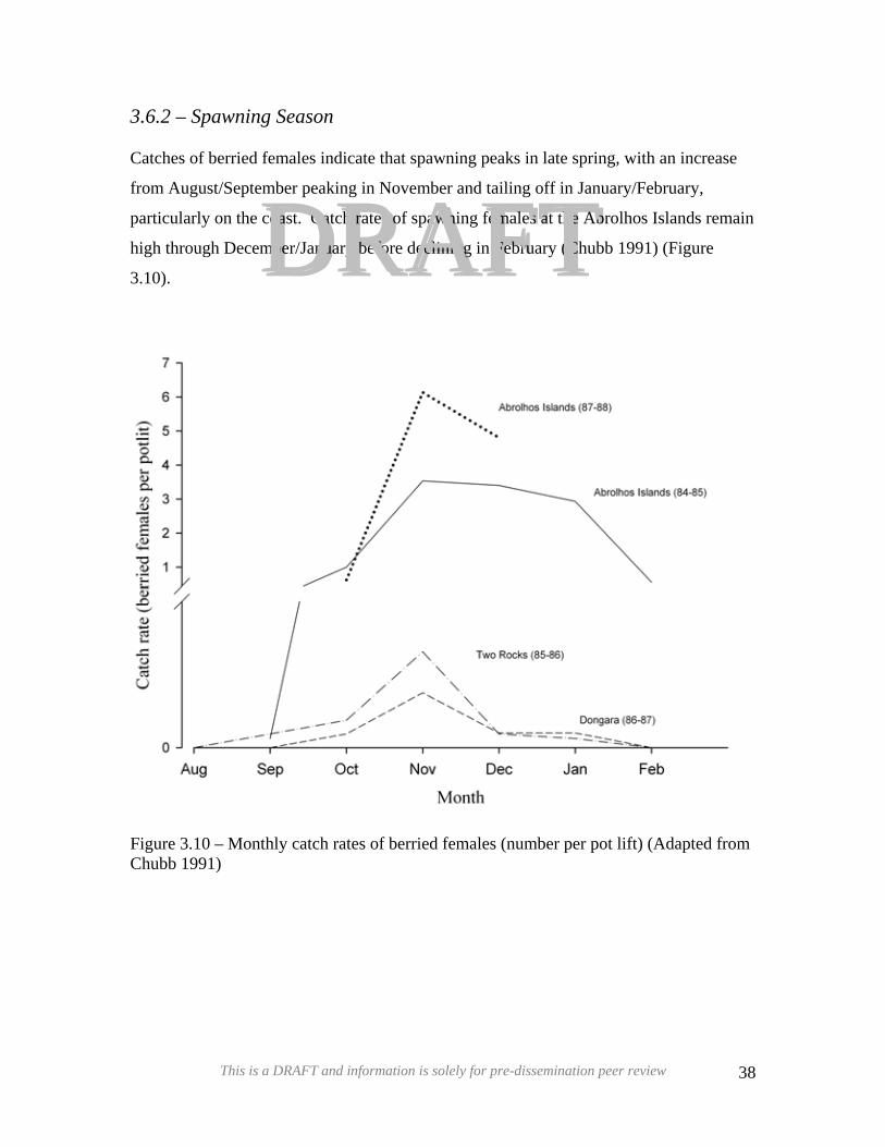
3.6.2 – Spawning Season
DRAFTCatches of berried females indicate that spawning peaks in late spring, with an increase
from August/September peaking in November and tailing off in January/February,
particularly on the coast. Catch rates of spawning females at the Abrolhos Islands remain
high through December/January before declining in February (Chubb 1991) (Figure
3.10). DRAFT
Figure 3.10 – Monthly catch rates of berried females (number per pot lift) (Adapted from Chubb 1991)
This is a DRAFT and information is solely for pre-dissemination peer review 38
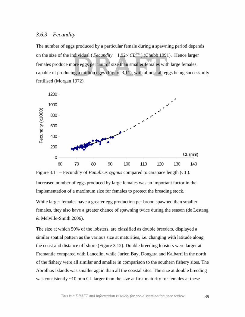
3.6.3 – Fecundity
DDRRAAFFTTThe number of eggs produced by a particular female during a spawning period depends
on the size of the individual ( ) (Chubb 1991). Hence larger
females produce more eggs per unit of size than smaller females with large females
capable of producing a million eggs (Figure 3.11), with almost all eggs being successfully
fertilised (Morgan 1972).
69.292.1 CLFecundity ×=
0
200
400
600
800
1000
1200
60 70 80 90 100 110 120 130 140
CL (mm)
Fecu
ndity
(x10
00)
Figure 3.11 – Fecundity of Panulirus cygnus compared to carapace length (CL).
Increased number of eggs produced by large females was an important factor in the
implementation of a maximum size for females to protect the breading stock.
While larger females have a greater egg production per brood spawned than smaller
females, they also have a greater chance of spawning twice during the season (de Lestang
& Melville-Smith 2006).
The size at which 50% of the lobsters, are classified as double breeders, displayed a
similar spatial pattern as the various size at maturities, i.e. changing with latitude along
the coast and distance off shore (Figure 3.12). Double breeding lobsters were larger at
Fremantle compared with Lancelin, while Jurien Bay, Dongara and Kalbarri in the north
of the fishery were all similar and smaller in comparison to the southern fishery sites. The
Abrolhos Islands was smaller again than all the coastal sites. The size at double breeding
was consistently ~10 mm CL larger than the size at first maturity for females at these
This is a DRAFT and information is solely for pre-dissemination peer review 39
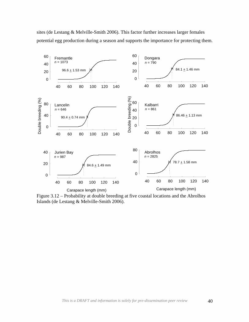
DDRRAAFFTTsites (de Lestang & Melville-Smith 2006). This factor further increases larger females
Figure 3.12 – Probability at double breeding at five coastal locations and the Abrolhos
potential egg production during a season and supports the importance for protecting them.
Islands (de Lestang & Melville-Smith 2006).
Fremantle
40 60 80 100 120 140
0
20
40
60
Kalbarri
40 60 80 100 120 140Dou
ble
bree
ding
(%)
0
20
40
60
Jurien Bay
Carapace length (mm)
40 60 80 100 120 140
0
20
40
Dongara
40 60 80 100 120 140
0
20
40
60
Abrolhos
Carapace length (mm)
40 60 80 100 120 140
0
40
80
Lancelin
40 60 80 100 120 140Dou
ble
bree
ding
(%)
0
40
80
86.46 + 1.13 mm
78.7 + 1.58 mm
84.1 + 1.46 mm
84.6 + 1.49 mm
90.4 + 0.74 mm
96.6 + 1.53 mm
n = 1073 n = 790
n = 646 n = 861
n = 987 n = 2825
This is a DRAFT and information is solely for pre-dissemination peer review 40

3.7 – Juvenile Recruitment
DDRRAAFFTTMost lobster larvae do not survive their long oceanic journey. Many are eaten by
predators or are not carried close enough to the shallow reefs by the ocean currents to
allow them to settle. Therefore, the number settling can vary greatly from year to year,
largely as a result of changes in environmental factors (Caputi et al. 2000). When the
Leeuwin Current is flowing strongly, a higher proportion of the larval lobsters return to
the coast. Westerly winds at the time of year when the puerulus are ready to settle may
also help more to reach the shallow reefs along the coast. One factor, which affects the
strength of the Leeuwin Current (and hence the level of pueruli settlement), is the
frequency of El Niños events. The occurrence of an El Niño reduces the strength of the
Leeuwin Current, with strong Leeuwin Currents resulting in better settlement of puerulus
(Caputi et. al. 1995b). A possible explanation for this relationship is that the warmer
oceanic waters may increase the development rate and survival of phyllosoma larvae.
The settlement of pueruli occurs through out the year, with peaks occurring in late winter
to mid summer (Figure 4.2), and generally at night, around each new moon.
The Department of Fisheries monitors the highly variable recruitment of puerulus to the
Abrolhos Islands and the coastal reefs on a monthly basis. This data is used as an index of
future stock levels providing a prediction of future catches three to four years in advance
(Sections 4.1 and 5.2).
This is a DRAFT and information is solely for pre-dissemination peer review 41

3.8 – Age and Growth
DDRRAAFFTTThe first assessments of P. cygnus growth rates were conducted under controlled aquaria
conditions (Chittleborough 1974b, 1976b) focusing on such effects as temperature,
photoperiod, oxygen, food supply, crowding, autonomy of limbs, and size at maturity.
Comparisons were also made between laboratory reared and wild populations
(Chittleborough 1975), with wild populations being studied through tag recapture
techniques (Chittleborough 1975, Morgan 1977). These data were used to attain estimates
of growth parameters for use in assessment models (Phillips et al. 1992, Hall & Chubb
2001). The modeling of tagging data remains the main techniques for determining growth
in western rock lobster.
Since 1992, the majority of tagging of lobsters has occurred in October and November by
Department of Fisheries staff at the conclusion of the IBSS (Section 4.3). The primary
focus of this tagging program has been to monitor year-to-year variability in moult
increments. Additional tagging has also occurred on a far more ad-hoc basis, with the
main focus being overall growth rates and movement patterns. For example in 1992, as
part of a migration study, undersize lobsters were tagged during the season with most
being caught soon after release. These provided little information on lobster growth.
3.8.1 – Methods
Growth may be underestimated from tagging due to reduced growth from injury induced
by tagging (Hunt and Lyons 1986), leg loss (Brown and Caputi 1986) or if lobsters that
moult less frequently preferentially retain tags (Muller et al. 2007). In addition, if
animals with very small growth increments are rejected from the analysis this may lead to
overestimation of growth. Consequently, a non-aggressive approach was taken to the
initial “clean-up” of the data. All data with very short times-at-liberty (< 90 days) has
proven detrimental for growth determination and has been removed from the dataset. All
lobsters retrieved with missing or regenerated limbs (Melville-Smith & de Lestang,
2007c) were also removed from the analysis.
The analysis by Stephenson and de Lestang (in prep) was based on the assumption that
growth is different between the sexes and changes with water temperature at different
This is a DRAFT and information is solely for pre-dissemination peer review 42
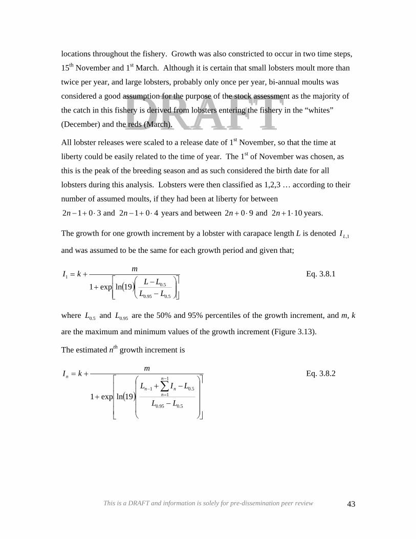
DDRRAAFFTTlocations throughout the fishery. Growth was also constricted to occur in two time steps,
15th November and 1st March. Although it is certain that small lobsters moult more than
twice per year, and large lobsters, probably only once per year, bi-annual moults was
considered a good assumption for the purpose of the stock assessment as the majority of
the catch in this fishery is derived from lobsters entering the fishery in the “whites”
(December) and the reds (March).
All lobster releases were scaled to a release date of 1st November, so that the time at
liberty could be easily related to the time of year. The 1st of November was chosen, as
this is the peak of the breeding season and as such considered the birth date for all
lobsters during this analysis. Lobsters were then classified as 1,2,3 … according to their
number of assumed moults, if they had been at liberty for between
years and between 4012and3012 ⋅+−⋅+− nn 1012and902 ⋅+⋅+ nn years.
The growth for one growth increment by a lobster with carapace length L is denoted
and was assumed to be the same for each growth period and given that;
1,LI
( )⎥⎥⎦
⎤
⎢⎢⎣
⎡⎟⎟⎠
⎞⎜⎜⎝
⎛−
−+
+=
5.095.0
5.01
19lnexp1LL
LLmkI Eq. 3.8.1
where and are the 50% and 95% percentiles of the growth increment, and m, k
are the maximum and minimum values of the growth increment (Figure 3.13).
5.0L 95.0L
The estimated nth growth increment is
( )⎥⎥⎥⎥
⎦
⎤
⎢⎢⎢⎢
⎣
⎡
⎟⎟⎟⎟
⎠
⎞
⎜⎜⎜⎜
⎝
⎛
−
−++
+=
∑−
=−
5.095.0
5.0
1
11
19lnexp1LL
LIL
mkIn
nnn
n Eq. 3.8.2
This is a DRAFT and information is solely for pre-dissemination peer review 43
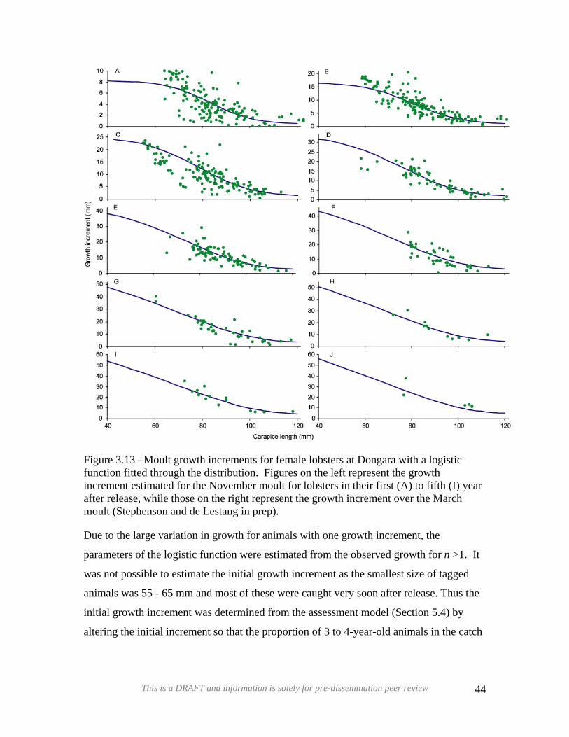
DDRRAAFFTT
Figure 3.13 –Moult growth increments for female lobsters at Dongara with a logistic function fitted through the distribution. Figures on the left represent the growth increment estimated for the November moult for lobsters in their first (A) to fifth (I) year after release, while those on the right represent the growth increment over the March moult (Stephenson and de Lestang in prep).
Due to the large variation in growth for animals with one growth increment, the
parameters of the logistic function were estimated from the observed growth for n >1. It
was not possible to estimate the initial growth increment as the smallest size of tagged
animals was 55 - 65 mm and most of these were caught very soon after release. Thus the
initial growth increment was determined from the assessment model (Section 5.4) by
altering the initial increment so that the proportion of 3 to 4-year-old animals in the catch
This is a DRAFT and information is solely for pre-dissemination peer review 44
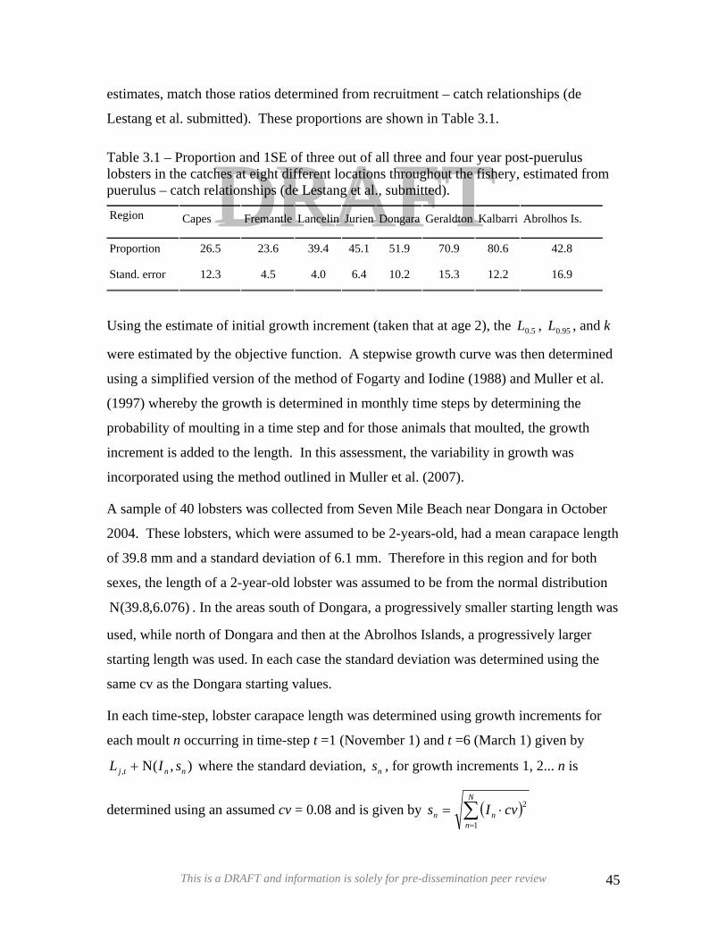
estimates, match those ratios determined from recruitment – catch relationships (de
Lestang et al. submitted). These proportions are shown in Table 3.1.
DDRRAAFFTTTable 3.1 – Proportion and 1SE of three out of all three and four year post-puerulus lobsters in the catches at eight different locations throughout the fishery, estimated from puerulus – catch relationships (de Lestang et al., submitted).
Region Capes Fremantle Lancelin Jurien Dongara Geraldton Kalbarri Abrolhos Is.
Proportion 26.5 23.6 39.4 45.1 51.9 70.9 80.6 42.8
Stand. error 12.3 4.5 4.0 6.4 10.2 15.3 12.2 16.9
Using the estimate of initial growth increment (taken that at age 2), the , , and k
were estimated by the objective function. A stepwise growth curve was then determined
using a simplified version of the method of Fogarty and Iodine (1988) and Muller et al.
(1997) whereby the growth is determined in monthly time steps by determining the
probability of moulting in a time step and for those animals that moulted, the growth
increment is added to the length. In this assessment, the variability in growth was
incorporated using the method outlined in Muller et al. (2007).
5.0L 95.0L
A sample of 40 lobsters was collected from Seven Mile Beach near Dongara in October
2004. These lobsters, which were assumed to be 2-years-old, had a mean carapace length
of 39.8 mm and a standard deviation of 6.1 mm. Therefore in this region and for both
sexes, the length of a 2-year-old lobster was assumed to be from the normal distribution
. In the areas south of Dongara, a progressively smaller starting length was
used, while north of Dongara and then at the Abrolhos Islands, a progressively larger
starting length was used. In each case the standard deviation was determined using the
same cv as the Dongara starting values.
)076.6,8.39(N
In each time-step, lobster carapace length was determined using growth increments for
each moult n occurring in time-step t =1 (November 1) and t =6 (March 1) given by
where the standard deviation, , for growth increments 1, 2... n is
determined using an assumed cv = 0.08 and is given by
),(N, nntj sIL + ns
( )∑=
⋅=N
nnn cvIs
1
2
This is a DRAFT and information is solely for pre-dissemination peer review 45

DDRRAAFFTTA Bayesian procedure was used to model the uncertainty in growth. A joint probability
distribution was generated using the Markov Chain Monte Carlo (MCMC) procedure in
AD Model Builder. Saving every 500th from 1250,000 cycles of the MCMC and
rejecting the first 500 generated during the burn-in period obtained a subset of 2000
values from the joint posterior distribution. The median and the 95% confidence limits
from the MCMC are shown in Figure 3.14 a & b.
This is a DRAFT and information is solely for pre-dissemination peer review 46
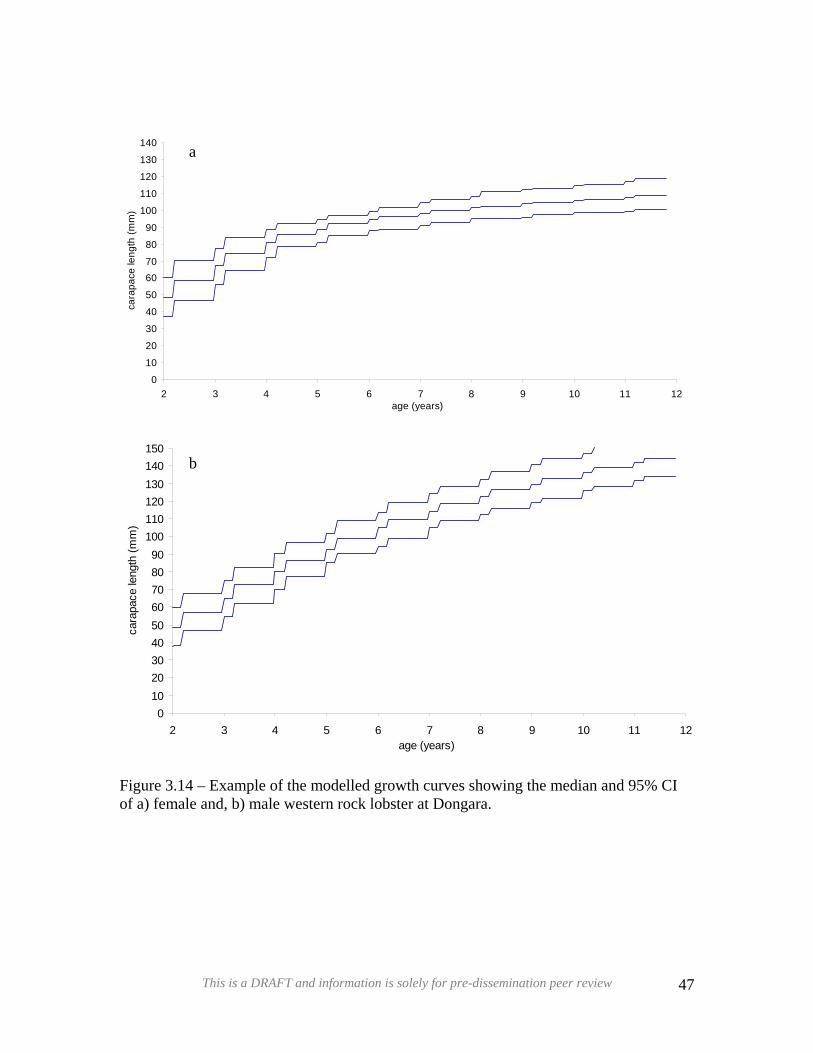
0
10
20
30
40
50
6070
80
90
100
110
120
130
140
2
cara
pace
leng
th (m
m)
0102030405060708090
100110120130140150
2
cara
pace
leng
th (m
m)
Figure 3.1of a) fema
a
DDRRAAFFTT3 4 5 6 7 8 9 10 11 12
age (years)
b3 4 5 6 7 8 9 10 11 1age (years)
2
4 – Example of the modelled growth curves showing the median and 95% CI le and, b) male western rock lobster at Dongara.
This is a DRAFT and information is solely for pre-dissemination peer review 47
3.9 – Diet
DRAFTThe western rock lobster is an opportunistic omnivore feeding on a wide range of food
items from coralline algae to molluscan and crustacean fauna (Joll & Phillips 1984, Edgar
1990) populations, which probably have high productivity, high turnover rates and short
life cycles. Studies have found that juvenile rock lobsters show a range of diets and
feeding strategies, varying greatly between seasons and between different habitats in the
same season (Edgar 1990). Edgar (1990) reported that the diet of P. cygnus reflected the
abundance and size distribution of benthic macrofauna available on all sampling
occasions
DRAFTInvestigation into the diet of adult western rock lobster populations in deep coastal
ecosystems (36 – 75 m) is currently underway (Waddington et al. in prep), using gut
content and stable isotope analysis. Results to date suggest that lobsters are primarily
carnivorous and act as secondary consumers. This same study also suggests a dietary shift
occurs upon migration from an omnivorous diet in shallow inshore areas, to a primarily
carnivorous diet in deep coastal ecosystems. Major prey items of lobsters in deep coastal
ecosystems include crabs, amphipods and isopods, with diet largely reflecting the food
availability of those taxa found free living or associated with algae on the benthos in
areas lobsters are known to forage. Dietary analysis also indicated that bait (pilchards) is
an important component of lobster diet at the locations investigated. Bait is available to
the lobsters through discards from fishing boats and by lobsters feeding on bait in pots
then exiting through the neck or through escape gaps in the case of undersize lobsters.
There is no evidence that lobster size or sex affects lobster diet or trophic position in deep
coastal ecosystems (size range investigated 65 – 120 mm CL) (Waddington et al. in
prep).
This is a DRAFT and information is solely for pre-dissemination peer review 48
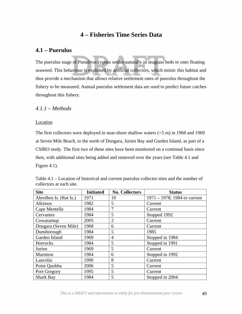
4 – Fisheries Time Series Data
DRAFTDRAFTThe puerulus stage of Panulirus cygnus settles naturally in seagrass beds or onto floating
seaweed. This behaviour is exploited by artificial collectors, which mimic this habitat and
thus provide a mechanism that allows relative settlement rates of puerulus throughout the
fishery to be measured. Annual puerulus settlement data are used to predict future catches
throughout this fishery.
4.1 – Puerulus
4.1.1 – Methods
Location
The first collectors were deployed in near-shore shallow waters (<5 m) in 1968 and 1969
at Seven Mile Beach, to the north of Dongara, Jurien Bay and Garden Island, as part of a
CSIRO study. The first two of these sites have been monitored on a continual basis since
then, with additional sites being added and removed over the years (see Table 4.1 and
Figure 4.1).
Table 4.1 – Location of historical and current puerulus collector sites and the number of collectors at each site.
Site Initiated No. Collectors Status Abrolhos Is. (Rat Is.) 1971 10 1971 – 1978; 1984 to current Alkimos 1982 5 Current Cape Mentelle 1984 7 Current Cervantes 1984 5 Stopped 1992 Cowaramup 2005 2 Current Dongara (Seven Mile) 1968 6 Current Dunsborough 1984 5 1985 Garden Island 1969 4 Stopped in 1984 Horrocks 1984 5 Stopped in 1991 Jurien 1969 5 Current Marmion 1984 6 Stopped in 1992 Lancelin 1990 8 Current Point Quobba 2006 5 Current Port Gregory 1995 5 Current Shark Bay 1984 5 Stopped in 2004
This is a DRAFT and information is solely for pre-dissemination peer review 49
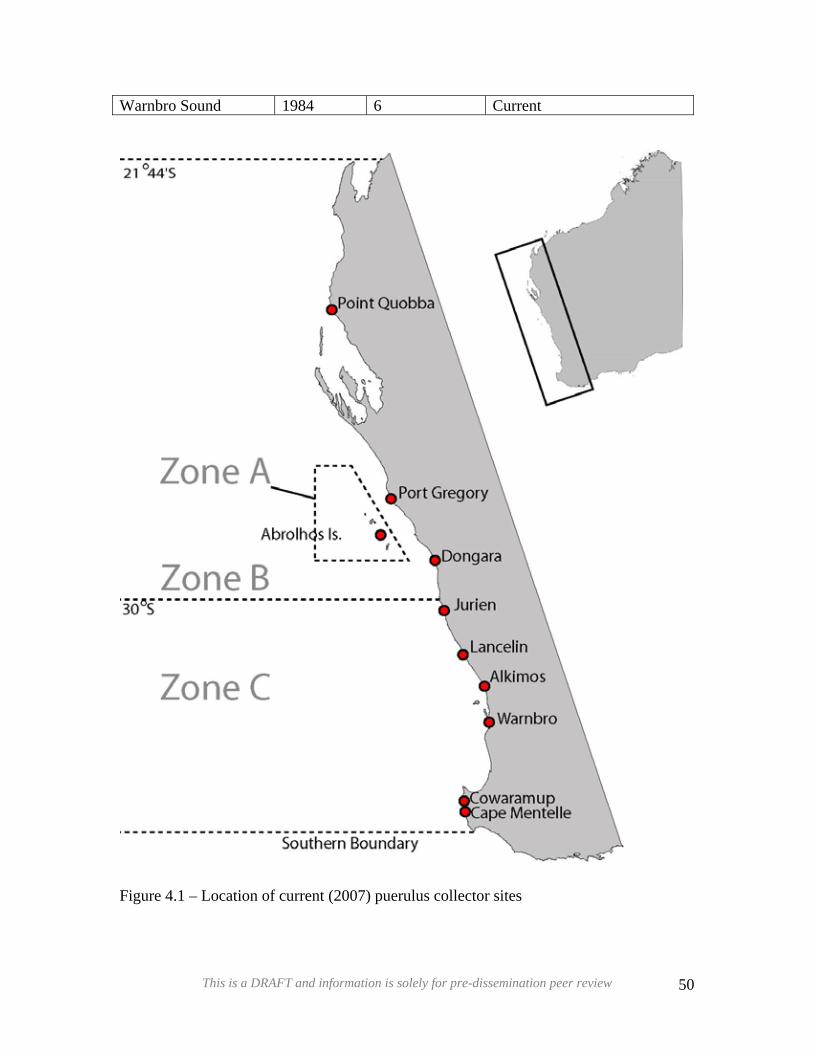
Warnbro Sound 1984 6 Current
DDRRAAFFTT
Figure 4.1 – Location of current (2007) puerulus collector sites
This is a DRAFT and information is solely for pre-dissemination peer review 50
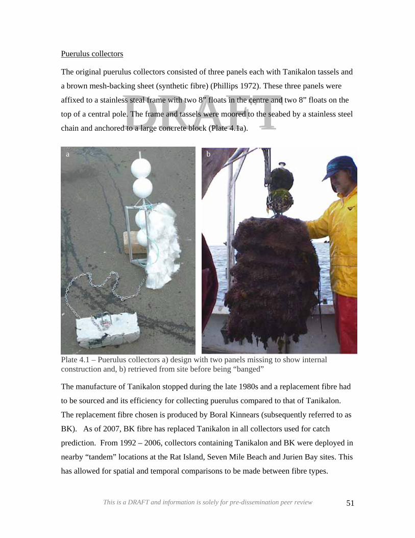
Puerulus collectors
DDRRAAFFTTThe original puerulus collectors consisted of three panels each with Tanikalon tassels and
a brown mesh-backing sheet (synthetic fibre) (Phillips 1972). These three panels were
affixed to a stainless steal frame with two 8” floats in the centre and two 8” floats on the
top of a central pole. The frame and tassels were moored to the seabed by a stainless steel
chain and anchored to a large concrete block (Plate 4.1a).
a b
Plate 4.1 – Puerulus collectors a) design with two panels missing to show internal construction and, b) retrieved from site before being “banged”
The manufacture of Tanikalon stopped during the late 1980s and a replacement fibre had
to be sourced and its efficiency for collecting puerulus compared to that of Tanikalon.
The replacement fibre chosen is produced by Boral Kinnears (subsequently referred to as
BK). As of 2007, BK fibre has replaced Tanikalon in all collectors used for catch
prediction. From 1992 – 2006, collectors containing Tanikalon and BK were deployed in
nearby “tandem” locations at the Rat Island, Seven Mile Beach and Jurien Bay sites. This
has allowed for spatial and temporal comparisons to be made between fibre types.
This is a DRAFT and information is solely for pre-dissemination peer review 51
DDRRAAFFTTTo further address the catchability differences between the two tassel types and various
backing materials, additional studies have been developed, one at Lancelin and another at
Seven Mile Beach. At Lancelin three puerulus collectors were deployed in October 2004.
The three panels on each collector contained different backing materials, one sheet using
the traditional brown material, a second sheet using the new white material and the third
sheet having no backing material. Preliminary analysis of this data indicates that the
puerulus catches on sheets with BK fibre tassels and no backing are not significantly
different (p > 0.05) from those backed with the traditional brown backing. Catches
produced by sheets covered with the new white material were significantly lower (p <
0.001) than the other two treatments.
Furthermore, the material used on the backing sheets, which originally was a brown
material glued onto the external side of the plastic backing sheets to provide additional
surface for puerulus to cling to, also ceased manufacture during the early 1990s, and a
replacement for this has also had to be sourced.
The second study, set up at Seven Mile Beach in July 2005 focused on both tassel types
and backing material. Six Phillips collectors were set in pairs of two (making three
groups). Of the six collectors, two were entirely fitted with Tanikalon fibres and brown
backing, two with BK fibres and brown backing and the final two, with BK fibres and no
backing material. Each month the position of each collector was randomly re-assigned to
one of these six locations to provide multiple pair-wise comparisons between different
collectors with different fibres in different locations. Preliminary analyses of these data
indicate that tassel type (p < 0.001) and not backing material (p > 0.05) (traditional brown
or no backing) significantly affects puerulus settlement rates. A conversion rate
determined from this analyses suggests that Tanikalon is ~ 20% more efficient than BK.
However, as this data set is relatively small, more data is being collected, and the
conversion factor does not explain the differences between the puerulus catch rates from
the other trials at Rat Island, Seven Mile Beach and Jurien Bay, no conversion factor is
currently being used to adjust puerulus settlement rates from BK fibres for use in catch
prediction. This work is on going.
This is a DRAFT and information is solely for pre-dissemination peer review 52
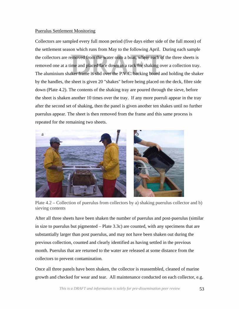
Puerulus Settlement Monitoring
DDRRAAFFTTCollectors are sampled every full moon period (five days either side of the full moon) of
the settlement season which runs from May to the following April. During each sample
the collectors are removed from the water onto a boat, where each of the three sheets is
removed one at a time and placed face down in a rack for shaking over a collection tray.
The aluminium shaker frame is slid over the P.V.C. backing board and holding the shaker
by the handles, the sheet is given 20 "shakes" before being placed on the deck, fibre side
down (Plate 4.2). The contents of the shaking tray are poured through the sieve, before
the sheet is shaken another 10 times over the tray. If any more pueruli appear in the tray
after the second set of shaking, then the panel is given another ten shakes until no further
puerulus appear. The sheet is then removed from the frame and this same process is
repeated for the remaining two sheets.
Plasie
Af
in
sub
pre
mo
co
On
gro
a
te 4.2 – Collection of puerulus from collectors by ving contents
ter all three sheets have been shaken the number of
size to puerulus but pigmented – Plate 3.3c) are co
stantially larger than post puerulus, and may not h
vious collection, counted and clearly identified as
nth. Puerulus that are returned to the water are rele
llectors to prevent contamination.
ce all three panels have been shaken, the collector
wth and checked for wear and tear. All maintenan
This is a DRAFT and information is solely for pr
b
a) shaking puerulus collector and b)
puerulus and post-puerulus (similar
unted, with any specimens that are
ave been shaken out during the
having settled in the previous
ased at some distance from the
is reassembled, cleaned of marine
ce conducted on each collector, e.g.
e-dissemination peer review 53
DDRRAAFFTTOther recordings made whilst at each site include a measure of surface water temperature
at the southern and northern ends of the collectors for that site, as well as a single
recording of salinity. One collector at each site is also fitted with an archival data storage
logger that records water temperatures. This continually records the water temperature
on an hourly basis and is removed and replaced with a new logger every second month.
replacement of one or more sheets, is also recorded. Department of Fisheries staff
currently conduct all servicing of the collectors from Warnbro Sound to Port Gregory,
with collectors at the extreme north (Point Quobba) and south (Cape Mentelle and
Cowaramup) of the fishery, being serviced by locally contracted people.
The environmental data and puerulus numbers are stored in an SQL based database. This
database is used to construct monthly and annual trends of puerulus settlement (Figure
4.4 and 4.5).
Analysis
Puerulus settlement indices in each management zone (Figure 2.1) are based on one or
more puerulus collection site (Table 4.2). Each index is the sum of the average number
of puerulus sampled per collector at each site over the settlement season (May to the
following April). Since the southern zone (C) uses data from more than one puerulus
location, a least squares mean estimate, standardised for location, is determined by GLM
with location, season and month as factors. In cases when a location was not serviced for
a given month(s), due to bad weather etc., an estimate of settlement is determined based
on the proportion that month contributes on average. Actual adjustments that have been
made to the data are 1988/89 Alkimos/0.64, 1989/90 Alkimos/0.97, 1989/90
Cervantes/0.77, 1968/69 Dongara/0.94, 1969/70 Cervanties/0.98 and 2000/01
Lancelin/0.82. 1968/69 Jurien is estimated from Dongara. At some locations additional
collectors have been added over the years for various reasons. To maintain the
consistency of the indices produced from these sites, additional collectors added over the
years are not used in the analysis (Table 4.2).
This is a DRAFT and information is solely for pre-dissemination peer review 54
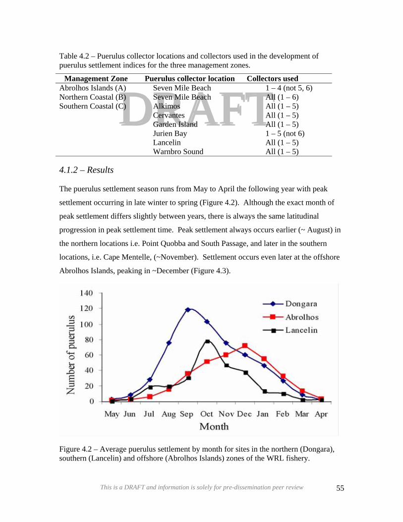
Table 4.2 – Puerulus collector locations and collectors used in the development of puerulus settlement indices for the three management zones.
DDRRAAFFTTManagement Zone Puerulus collector location Collectors used
Abrolhos Islands (A) Seven Mile Beach 1 – 4 (not 5, 6) Northern Coastal (B) Seven Mile Beach All (1 – 6) Southern Coastal (C) Alkimos All (1 – 5) Cervantes All (1 – 5) Garden Island All (1 – 5) Jurien Bay 1 – 5 (not 6) Lancelin All (1 – 5) Warnbro Sound All (1 – 5)
4.1.2 – Results
The puerulus settlement season runs from May to April the following year with peak
settlement occurring in late winter to spring (Figure 4.2). Although the exact month of
peak settlement differs slightly between years, there is always the same latitudinal
progression in peak settlement time. Peak settlement always occurs earlier (~ August) in
the northern locations i.e. Point Quobba and South Passage, and later in the southern
locations, i.e. Cape Mentelle, (~November). Settlement occurs even later at the offshore
Abrolhos Islands, peaking in ~December (Figure 4.3).
Figure 4.2 – Average puerulus settlement by month for sites in the northern (Dongara), southern (Lancelin) and offshore (Abrolhos Islands) zones of the WRL fishery.
This is a DRAFT and information is solely for pre-dissemination peer review 55
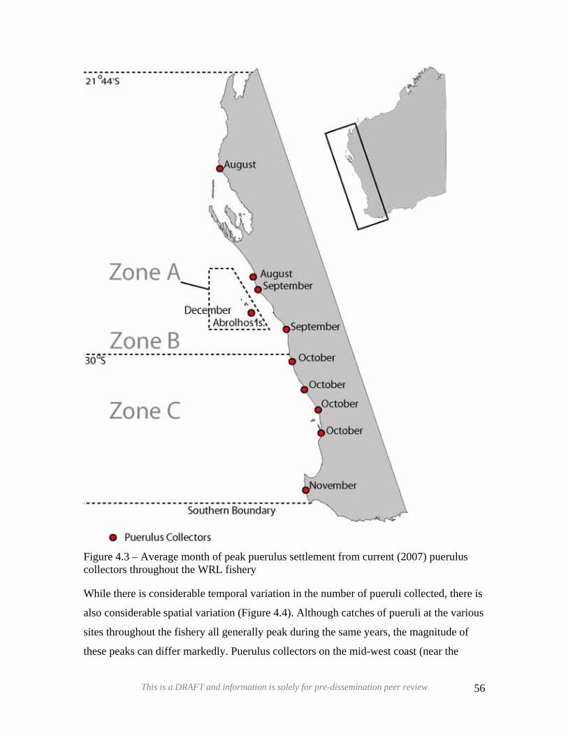
DDRRAAFFTT
Figure 4.3 – Average month of peak puerulus settlement from current (2007) puerulus collectors throughout the WRL fishery
While there is considerable temporal variation in the number of pueruli collected, there is
also considerable spatial variation (Figure 4.4). Although catches of pueruli at the various
sites throughout the fishery all generally peak during the same years, the magnitude of
these peaks can differ markedly. Puerulus collectors on the mid-west coast (near the
This is a DRAFT and information is solely for pre-dissemination peer review 56
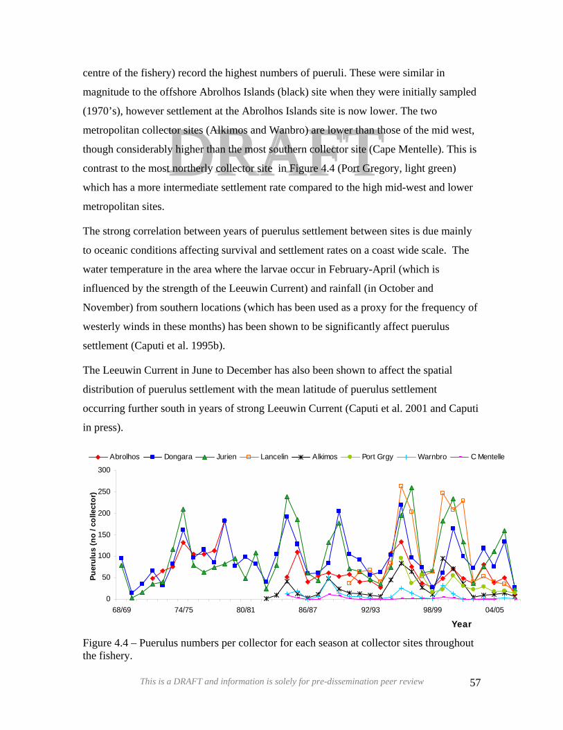
DDRRAAFFTTcentre of the fishery) record the highest numbers of pueruli. These were similar in
magnitude to the offshore Abrolhos Islands (black) site when they were initially sampled
(1970’s), however settlement at the Abrolhos Islands site is now lower. The two
metropolitan collector sites (Alkimos and Wanbro) are lower than those of the mid west,
though considerably higher than the most southern collector site (Cape Mentelle). This is
contrast to the most northerly collector site in Figure 4.4 (Port Gregory, light green)
which has a more intermediate settlement rate compared to the high mid-west and lower
metropolitan sites.
The strong correlation between years of puerulus settlement between sites is due mainly
to oceanic conditions affecting survival and settlement rates on a coast wide scale. The
water temperature in the area where the larvae occur in February-April (which is
influenced by the strength of the Leeuwin Current) and rainfall (in October and
November) from southern locations (which has been used as a proxy for the frequency of
westerly winds in these months) has been shown to be significantly affect puerulus
settlement (Caputi et al. 1995b).
The Leeuwin Current in June to December has also been shown to affect the spatial
distribution of puerulus settlement with the mean latitude of puerulus settlement
occurring further south in years of strong Leeuwin Current (Caputi et al. 2001 and Caputi
in press).
0
50
100
150
200
250
300
68/69 74/75 80/81 86/87 92/93 98/99 04/05
Year
Puer
ulus
(no
/ col
lect
or)
Abrolhos Dongara Jurien Lancelin Alkimos Port Grgy Warnbro C Mentelle
Figure 4.4 – Puerulus numbers per collector for each season at collector sites throughout the fishery.
This is a DRAFT and information is solely for pre-dissemination peer review 57
4.2 – Commercial Monitoring
DRAFTOn-board monitoring of commercial catches by Department of Fisheries staff was
initiated in 1971. This program involves members of the Research Division, making
regular and detailed records of the target catch (retained and returned to the sea) and by-
catch landings as well as environmental conditions and fishing activities. This program
provides vital information such as juvenile (undersize) and spawning stock abundance
and size at maturity on a broad temporal and spatial scale (Figure 4.5).
DRAFT4.2.1 – Methods
Location
Monitoring occurs every month throughout the fishing season (November – June) in four
main localities Dongara, Jurien, Lancelin and Fremantle since 1971 and more recently in
a further two locations, Kalbarri and the Abrolhos Islands (since 1985). Opportunistic
monitoring also occurs in other localities such as Mandurah and the Capes region (Figure
4.5). For each locality monitoring is only conducted onboard vessels fishing within 15
nm north or south of the target port.
Sampling
During each month, at each location, monitoring is spread across four depth categories,
i.e. <18, 18 –36, 36 – 54 and >54 m (<10, 10 – 20, 20 – 30 and >30 fathoms), with a
minimum sample of 300 individuals being sought in each depth range. Sampling in some
location-depth combinations in some months is missing due to vessels not fishing in that
depth range due to poor catches or weather conditions.
Information is recorded on an individual lobster basis and includes carapace length to the
nearest 1 mm, sex, breeding condition and colour (migratory white or sedentary red).
Information is also collected on the skipper and crew as well as the fishing vessel, fishing
techniques and interactions with non-target species (see Appendix1 for specifics). The
data are entered and stored on an SQL based database for analysis.
This is a DRAFT and information is solely for pre-dissemination peer review 58
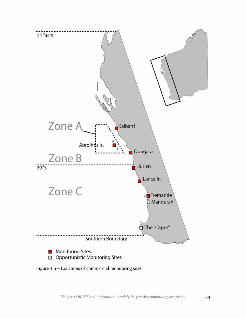
DDRRAAFFTT
Figure 4.5 – Locations of commercial monitoring sites
This is a DRAFT and information is solely for pre-dissemination peer review 59
Analysis
DDRRAAFFTTData from commercial monitoring is used to construct a number of annual indices, used
in the management of this fishery. These include breeding stock indices, a juvenile
(undersize) abundance index, coast wide water temperature trends, annual mean size of
the smallest 10% mature females, proportions moulting out of a setose phase each
autumn, octopus catch rates, and by-catch. Of these indices, the most important for use in
the management of this fishery is the breeding stock index.
Fishery-Dependent Breeding Stock Index.
Breeding stock indices (BSI) are produced for each of the two coastal regions, with
monitoring at Dongara and Jurien used to produce the north coastal index and data from
Lancelin and Fremantle used for the south coastal index. Each index is a Least Squared
Mean (LSM) of eggs per pot lift in the deep-water breeding grounds of the region during
the spawning season (September – February). The carapace length (CL) of each female
measured during commercial monitoring in deep water (>36 m in Zone B and >18 m in
Zone C) is converted to an estimated fecundity based on a size-fecundity relationship, a
size-maturity relationship, and a size-double breeding relationship (equations 4.2.1-5).
To account for a moult in February, the carapace lengths of all females measured after
this month (March – June) are reduced by 4 mm, as this reduces them to the size they
would have been during the previous spawning season (i.e. September – February). The
annual estimate of egg production is a back-transformed value produced from a GLM of
the logarithm of the number of eggs per pot lift, where fishing season, monitoring
location, sub-location nested within location, month and pot type are all treated as factors.
Water depth and water depth2 are employed as covariates and the model is weighted by
the number of pots sampled. A fishing efficiency of 1 – 2% pa is applied to the index to
take into account increases in efficiency associated with radar, colour echo sounders,
GPS, etc. (Table 5.1). Annual variations in catchability due to environmental conditions
are also taken into account by applying a 3-year moving average to the time series.
This is a DRAFT and information is solely for pre-dissemination peer review 60

The number of eggs in a single batch of eggs:
DDRRAAFF69.292.1 CLFecundity ×=
TT. Eq. 4.2.1
Probability that a female is mature:
( )( )CLPmatureZoneB ×−+= 203.077.18exp1/1 Eq. 4.2.2
( )( )2*0040.0987.051.59exp1/1 CLCLPmatureZoneC +×−+= Eq. 4.2.3
Probability that a female will spawn twice:
( )( )( )484.00495.0075.4exp1/11 +×−++= CLPdblspawnZoneB Eq. 4.2.4
( )( )( )484.00495.0075.4exp1/11 −×−++= CLPdblspawnZoneC Eq. 4.2.5
where CL is the carapace length. * The sizes at maturity and at double breeding
equations above are derived from Chubb 1991. New estimates of these parameters,
reported in section 3.6, will be incorporated into the model in the near future.
Biological Reference Points
The Breeding Stock Index (BSI) is measured against a lower threshold (Biological
Reference Point (BRP)). This point is equivalent to the BSI estimate for the 1980/81
fishing season, a period when the breeding stock was estimated by Hall and Chubb
(2001) to be ~ 20% of the virgin biomass, a level substantially higher than that recorded
during the early 1990s. Since, the breeding stock during the 1990s did not result in
recruitment over-fishing, the higher 1980s BRP can be considered a fairly conservative
level.
Index of Juvenile Abundance
Indices of juvenile abundance provide a qualitative assessment of recruitment to the
fishery. Two indices are produced for the both north and south coastal regions, based on
lobsters with carapace lengths < 68 mm and 68 – 76 mm (Figs 4.7a, b). These indices
provide information relative to recruitment into the fishery two and one years in advance,
respectively. These indices are Least Squared Means (LSM) of juveniles per pot lift in
shallow waters (< 36 m) collected at Dongara and Jurien Bay (North Coastal region) and
This is a DRAFT and information is solely for pre-dissemination peer review 61
DDRRAALancelin and Fremantle (South Coastal region). The indices are adjusted to account for
fishing efficiency increases (Table 5.1), as well as to account for the impact of increasing
the number of escape gaps (from one to three or four) in 1986/87. All data points after
1985/86 are multiplied by three and two for the < 68 mm and 68 – 76 mm indices,
respectively, to account for the escape gaps. FFTT4.2.2 – Results
Fishery-Dependent Breeding Stock Index.
Monitoring of the commercial catches saw a decline in the breeding stock index from its
inception in the early 1970s until 1992/93 (Figure 4.6). In the late 1980s, and early 1990s
the breeding stock indices fell below their respective threshold level (Section 2). This
decline prompted the introduction of the management changes designed at increasing the
breeding stock (Box 2.1 – 1993/94). This and subsequent management measures have led
to a recovery of the spawning stock in both the north and south of the fishery. However,
there has been a more recent decline in the spawning stock, particularly in the north
coastal region of the fishery, to levels just above the threshold BRP (Figure 4.6).
Index of Juvenile Abundance
For each coastal region the two indices of juvenile abundance (< 68 and 68-76 mm) show
very similar trends as they reflect the variable puerulus settlement two and three earlier
(Figs 4.7a,b). The past four seasons have shown a progressive decline in juvenile
abundance, with very low levels being recorded in the 2005/06 fishing season, especially
the 68 – 76 mm indices. These data suggests that commercial catches in coastal regions
during 2006/07 and 2007/08 will be below average. This re-iterates the scenario
estimated by the puerulus settlement indices for these seasons (Section 4.1 & 5.2).
This is a DRAFT and information is solely for pre-dissemination peer review 62
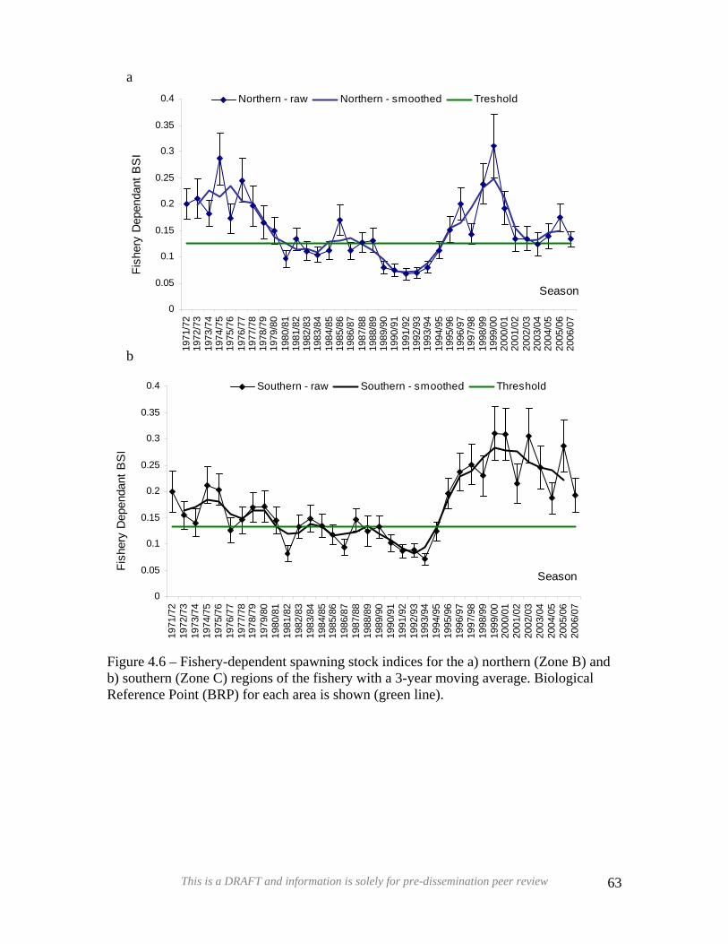
Figb) Re
a
DDRRAAFFTT0
0.05
0.1
0.15
0.2
0.25
0.3
0.35
0.4
1971
/72
1972
/73
1973
/74
1974
/75
1975
/76
1976
/77
1977
/78
1978
/79
1979
/80
1980
/81
1981
/82
1982
/83
1983
/84
1984
/85
1985
/86
1986
/87
1987
/88
1988
/89
1989
/90
1990
/91
1991
/92
1992
/93
1993
/94
1994
/95
1995
/96
1996
/97
1997
/98
1998
/99
1999
/00
2000
/01
2001
/02
2002
/03
2003
/04
2004
/05
2005
/06
2006
/07
Season
Fish
ery
Dep
enda
nt B
SI
Northern - raw Northern - smoothed Treshold
b0
0.05
0.1
0.15
0.2
0.25
0.3
0.35
0.4
1971
/72
1972
/73
1973
/74
1974
/75
1975
/76
1976
/77
1977
/78
1978
/79
1979
/80
1980
/81
1981
/82
1982
/83
1983
/84
1984
/85
1985
/86
1986
/87
1987
/88
1988
/89
1989
/90
1990
/91
1991
/92
1992
/93
1993
/94
1994
/95
1995
/96
1996
/97
1997
/98
1998
/99
1999
/00
2000
/01
2001
/02
2002
/03
2003
/04
2004
/05
2005
/06
2006
/07
Season
Fish
ery
Dep
enda
nt B
SI
Southern - raw Southern - smoothed Threshold
ure 4.6 – Fishery-dependent spawning stock indices for the a) northern (Zone B) and
southern (Zone C) regions of the fishery with a 3-year moving average. Biological ference Point (BRP) for each area is shown (green line).
This is a DRAFT and information is solely for pre-dissemination peer review 63
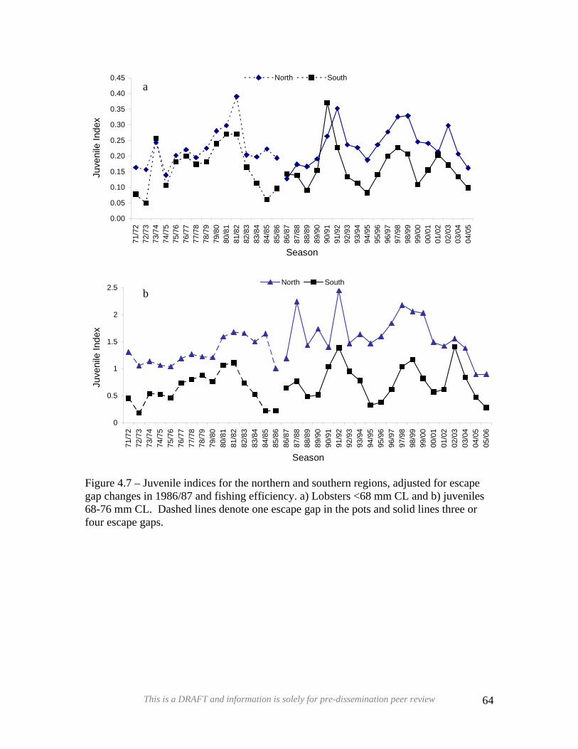
0.00
0.05
0.10
0.15
0.20
0.25
0.30
0.35
0.40
0.45
Juve
nile
Inde
x
North South
0
0.5
1
1.5
2
2.5
71/7
2
Juve
nile
Inde
x
Figure 4.7 –gap changes68-76 mm Cfour escape
a
DDRRAAFFTT71
/72
72/7
373
/74
74/7
575
/76
76/7
777
/78
78/7
979
/80
80/8
181
/82
82/8
383
/84
84/8
585
/86
86/8
787
/88
88/8
989
/90
90/9
191
/92
92/9
393
/94
94/9
595
/96
96/9
797
/98
98/9
999
/00
00/0
101
/02
02/0
303
/04
04/0
5
Season
North South
b72/7
373
/74
74/7
575
/76
76/7
777
/78
78/7
979
/80
80/8
181
/82
82/8
383
/84
84/8
585
/86
86/8
787
/88
88/8
989
/90
90/9
191
/92
92/9
393
/94
94/9
595
/96
96/9
797
/98
98/9
999
/00
00/0
101
/02
02/0
303
/04
04/0
505
/06
Season
Juvenile indices for the northern and southern regions, adjusted for escape in 1986/87 and fishing efficiency. a) Lobsters <68 mm CL and b) juveniles L. Dashed lines denote one escape gap in the pots and solid lines three or gaps.
This is a DRAFT and information is solely for pre-dissemination peer review 64
4.3 – Independent Breeding Stock Survey (IBSS)
DRAFTSince 1991, the Research Division of the Department of Fisheries has undertaken an
annual survey of the breeding stock. This survey provides fisheries managers with a
measure of the breeding stock, independent of the effects of increasing fishing efficiency
(Melville-Smith & de Lestang 2006), producing a cross check of the trends exhibited by
the fishery-dependent breeding stock index, which is a longer time series. DRAFT
4.3.1 – Methods
Sampling Locations
The IBSS is conducted over ten days during the last new moon before the
commencement of the fishery season (15th November). This period is also close to the
annual peak of egg production, which occurs in either October or November, depending
on moon phase (Chubb 1991: - Section 3.4). The IBSS involves the setting of standard
fishing pots in up to five coastal sites as well as the Abrolhos Islands using the same
locations each year. The survey runs annually at Dongara, Lancelin and the Abrolhos
Islands, as well as intermittently (every five years) at Fremantle, Jurien and Kalbarri
(Figure 4.8). Commercial WRL boats are chartered for all coastal locations, with the
Department of Fisheries research vessel undertaking research at the Abrolhos Islands.
For the coastal sites, surveys are undertaken at depths from 25 – 70 m while at the
Abrolhos Islands the depth range surveyed is 10 – 60 m. This corresponds to the depths at
which most breeding lobsters are found (Chubb 1991).
This is a DRAFT and information is solely for pre-dissemination peer review 65
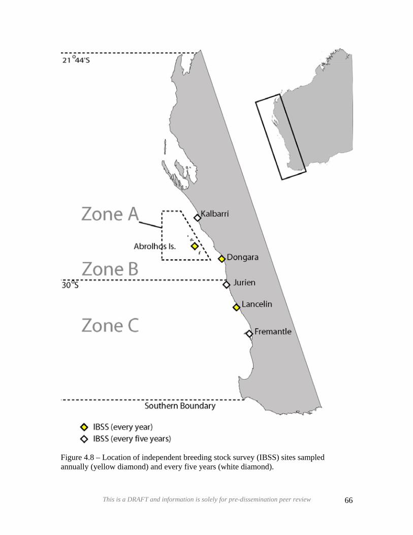
DDRRAAFFTT
Figure 4.8 – Location of independent breeding stock survey (IBSS) sites sampled annually (yellow diamond) and every five years (white diamond).
This is a DRAFT and information is solely for pre-dissemination peer review 66
Breeding Stock Sampling Regime
DDRRAAFFTTEach year 160 commercially sized batten pots, with no escape gaps, are used. These are
set up for a two-day pull, with 80 pots being sampled each day during the 10-day
sampling period for the coastal sites. At the Abrolhos Islands 51 pots are used with one
day pulls due to the greater quantity of lobsters that are caught. Standard baits of North
Sea Herring and salmon heads are used with standard amounts. Due to Australian
Quarantine regulations the North Sea Herring has been substituted with local Scaly
Mackerel in recent years. Anecdotal information from fishers indicates there should not
be an effect on catch rates. The data recorded are shown below in Appendix 2.
Tagging
After the completion of the IBSS sampling, there is an additional two days spent in the
shallows (<36 m) tagging lobster for growth and movement information. The tagging
protocol is outlined below, though results in terms of movement and growth are detailed
in section 3.5; 3.8).
Each year tagging in shallow waters is undertaken for two days after the IBSS at Dongara
and Lancelin. During each tagging day, all male lobsters caught with a carapace between
65 and 75 mm, and without missing appendages are tagged with a Hallprint ™ “standard
T-bar anchor tag” ventrally between the first and second abdominal segments (Plate 4.3).
This is a DRAFT and information is solely for pre-dissemination peer review 67
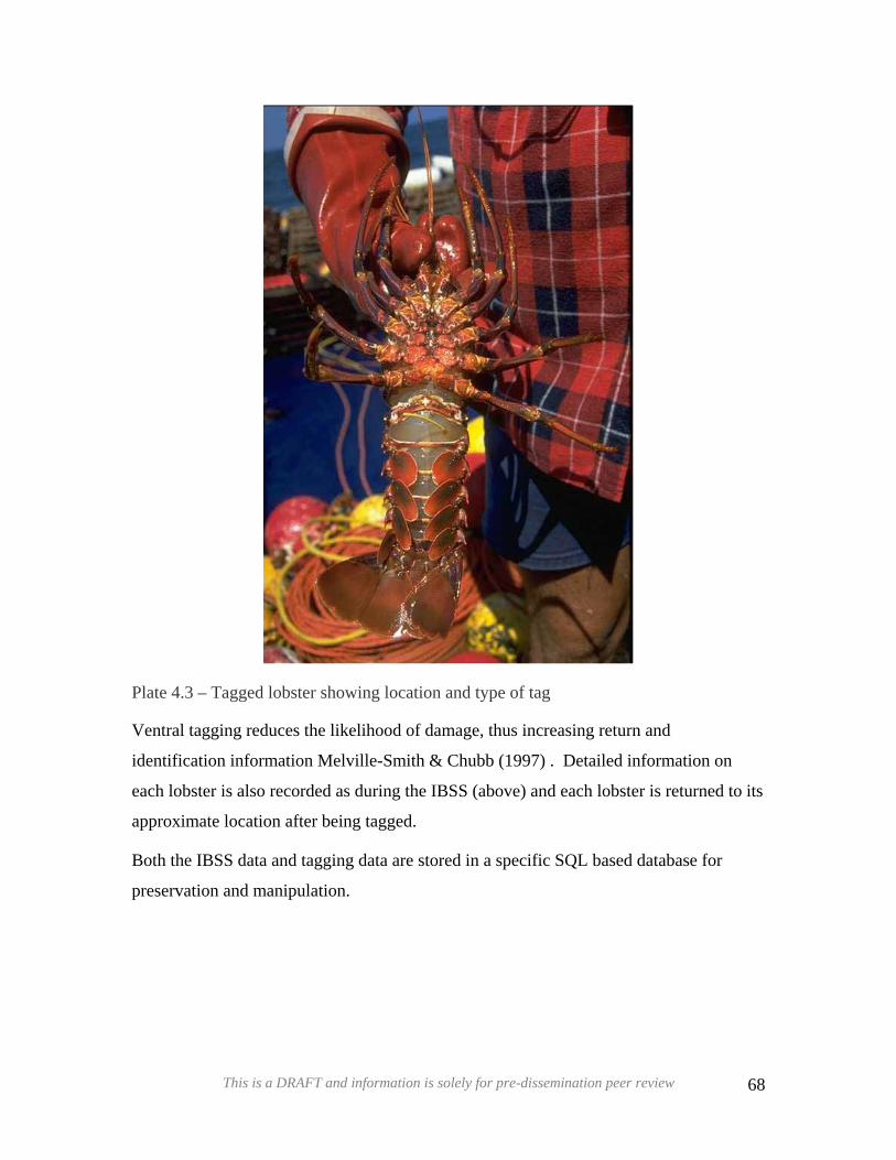
DDRRAAFFTT
Plate 4.3 – Tagged lobster showing location and type of tag
Ventral tagging reduces the likelihood of damage, thus increasing return and
identification information Melville-Smith & Chubb (1997) . Detailed information on
each lobster is also recorded as during the IBSS (above) and each lobster is returned to its
approximate location after being tagged.
Both the IBSS data and tagging data are stored in a specific SQL based database for
preservation and manipulation.
This is a DRAFT and information is solely for pre-dissemination peer review 68
Analysis
DDRRAAFFTTData from the IBSS is used to construct a number of annual indices, used in the
management of this fishery. These include the fishery independent BSI and, estimates of
female size at maturity. Of these indices, the most important for use in the management
of this fishery is the fishery independent BSI.
Fishery Independent Breeding Stock Index (BSI)
Breeding stock indices (BSI) are produced for the northern and southern coastal and
Abrolhos regions, with coastal surveys conducted at Kalbarri, Dongara and Jurien used to
produce the northern (Zone B) index and Lancelin and Fremantle used for the southern
(Zone C ) index. Each index is an adjusted Least Squares Mean (LSM) of eggs per pot
lift (SAS Institute Inc.). The carapace length (CL) of each “mature” female (ovigerous
setae – Figure 3.7b) is converted to an estimated seasonal fecundity based on a size-
fecundity relationship and a size-double breeding relationship (Chubb 1991: equations
4.3.1-4). The estimate of egg production is a back-transformed value of the LSM of the
factor, year, produced from a GLM of the log (number of eggs per pot lift), where year,
location, sub-location nested within location, pot type, depth category, day pull and swell
range, are all treated as factors.
The number of eggs in a single batch of eggs:
69.292.1 CLFecundity ×= . Eq. 4.3.1
Probability that a female will spawn twice:
( )( )( )484.00495.0075.4exp1/11 +×−++= CLPdblspawnZoneB Eq. 4.3.2
( )( )( )484.00495.0075.4exp1/11 −×−++= CLPdblspawnZoneC Eq. 4.3.3
( )(( )CLPdblspawnZoneA )×−++= 1063.0675.6exp1/11 Eq. 4.3.4
where CL is the carapace length.
This is a DRAFT and information is solely for pre-dissemination peer review 69
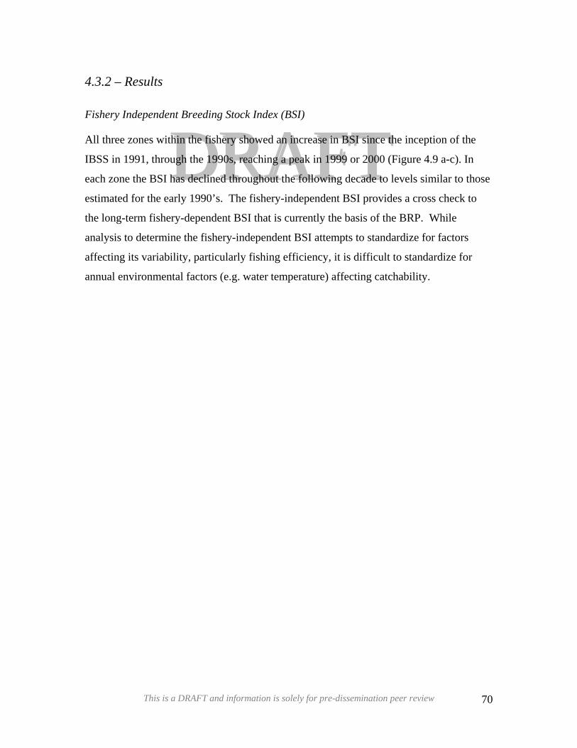
4.3.2 – Results
DDRRAAFFTTAll three zones within the fishery showed an increase in BSI since the inception of the
IBSS in 1991, through the 1990s, reaching a peak in 1999 or 2000 (Figure 4.9 a-c). In
each zone the BSI has declined throughout the following decade to levels similar to those
estimated for the early 1990’s. The fishery-independent BSI provides a cross check to
the long-term fishery-dependent BSI that is currently the basis of the BRP. While
analysis to determine the fishery-independent BSI attempts to standardize for factors
affecting its variability, particularly fishing efficiency, it is difficult to standardize for
annual environmental factors (e.g. water temperature) affecting catchability.
Fishery Independent Breeding Stock Index (BSI)
This is a DRAFT and information is solely for pre-dissemination peer review 70
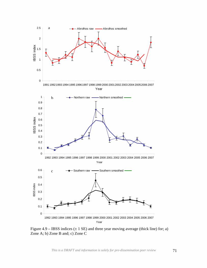
0
0.5
1
1.5
2
2.5
199
IBS
S in
dex
Abrolhos raw Abrolhos smoothed
0
0.1
0.2
0.3
0.4
0.5
0.6
0.7
0.8
0.9
1
19
IBS
S in
dex
0
0.1
0.2
0.3
0.4
0.5
0.6
19
IBSS
inde
x
Figure 4.9Zone A; b
a
DDRRAAFFTT1 19921993 1994 1995 19961997 1998 1999 2000 20012002 2003 2004 20052006 2007
Year
92
Northern raw Northern smoothed
92
–) Z
b
1993 1994 1995 1996 1997 1998 1999 2000 2001 2002 2003 2004 2005 2006 2007Year
Southern raw Southern smoothed
c1993 1994 1995 1996 1997 1998 1999 2000 2001 2002 2003 2004 2005 2006 2007Year
IBSS indices (± 1 SE) and three year moving average (thick line) for; a) one B and; c) Zone C
This is a DRAFT and information is solely for pre-dissemination peer review 71
4.4 – Volunteer Research Log Books
DRAFTFisheries Research Logbooks have been issued to fishers since 1963. They are given to
approximately 60% of commercial fishers each year with 30-40% of all fishers
completing the logbook. Returns from fishers varies between years, from a peak in
2002/03 of 41% of the whole fleet to current levels (2006/07) of around 28%. Over the
last 8 years, on average, 36% of the fleet have returned Research Logbooks, with almost
all (~90%) of those returning the logbook completing the voluntary section, which
provides additional information on catches and environmental conditions (Appendix 3).
The research logbooks provide the Department of Fisheries with detailed information on
commercial fishers’ practices, daily catch and effort by depth at a higher spatial
resolution than the CAES data. A summary of their catch rate is returned to individual
fishers at the end of the year with a comparison to the zone average.
DRAFT
Key indices produced from these logbook data include;
o Logbook catch and effort by 1o S transect in waters <20 and > 20 fm (36 m).
o Catch rate of spawners, setose and maximum size females that are returned to the
sea. An estimate of the total number of setose returned is obtained by weighing
up the logbook data to the total fishery (CAES data) where necessary.
o Catch rate of undersize lobsters.
o Daily index of swell height.
o Octopus catches and more recently, lobster mortalities.
4.4.1 – Methods
The logbooks are divided into two sections, a core section and a voluntary section
(Appendix 3). The data is stored in an SQL-based database that can be queried to
produce catch and effort statistics on fine spatial and temporal scales.
This is a DRAFT and information is solely for pre-dissemination peer review 72
4.4.2 – Results
DRAFTOver the last 20 years volunteer logbooks have provided data over much of the fishery
(Figure 4.10). Areas of high logbook returns correspond to areas of high fishing effort,
namely Big Bank (north of the Abrolhos Islands), Geraldton to Dongara, and the area
around Lancelin (north of Perth). This distribution is very similar for each individual
year, as shown by returns from the last fishing season (2005/06) (Figure 4.11). DRAFT
The large proportion of fishers that fill out logbooks and the spatial coverage of this data
means that general trends exhibited by the logbooks are representative of the general
fishing patterns that occur across the fishery. For example, the daily catch rates
determined from the research logbook program, showing as series of peaks and troughs
associated with changes in the fishery (whites to reds) and also lunar effects, are
representative of those that occur across the entire fleet (Figure 4.12).
This fact allows logbook data, which is recorded on a fine temporal and spatial scale, to
be used pro-rata to divide-up CAES data into finer scales than their reported monthly
time steps and 1o blocks (Section 4.5).
The logbooks also provide data additional to that recorded by other data sources,
including the numbers of setose females captured and returned to the water. The return
of setose females was a management initiative introduced in 1992/93 (Box 2.1). Since
then the numbers of setose females returned have been recorded as part of the volunteer
research logbook program.
These data show that there has been an overall increase in the weight of setose females
returned in all three zones up until this most recent season (2006/07) (Figure 4.13). Both
coastal zones peaked during 1999/00 with the recorded catches, and decreased slightly
over the next few years. There was a recovery in all three zones in the early 2000s,
however Zone B has declined since 2004/05, with Zones A and C falling this year, and
Zone C markedly.
This is a DRAFT and information is solely for pre-dissemination peer review 73
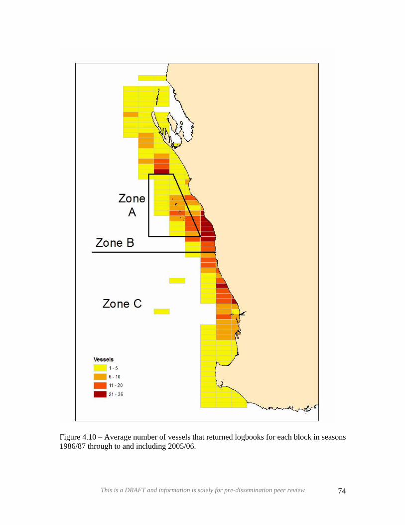
DDRRAAFFTT
Figure 4.10 – Average number of vessels that returned logbooks for each block in seasons 1986/87 through to and including 2005/06.
This is a DRAFT and information is solely for pre-dissemination peer review 74
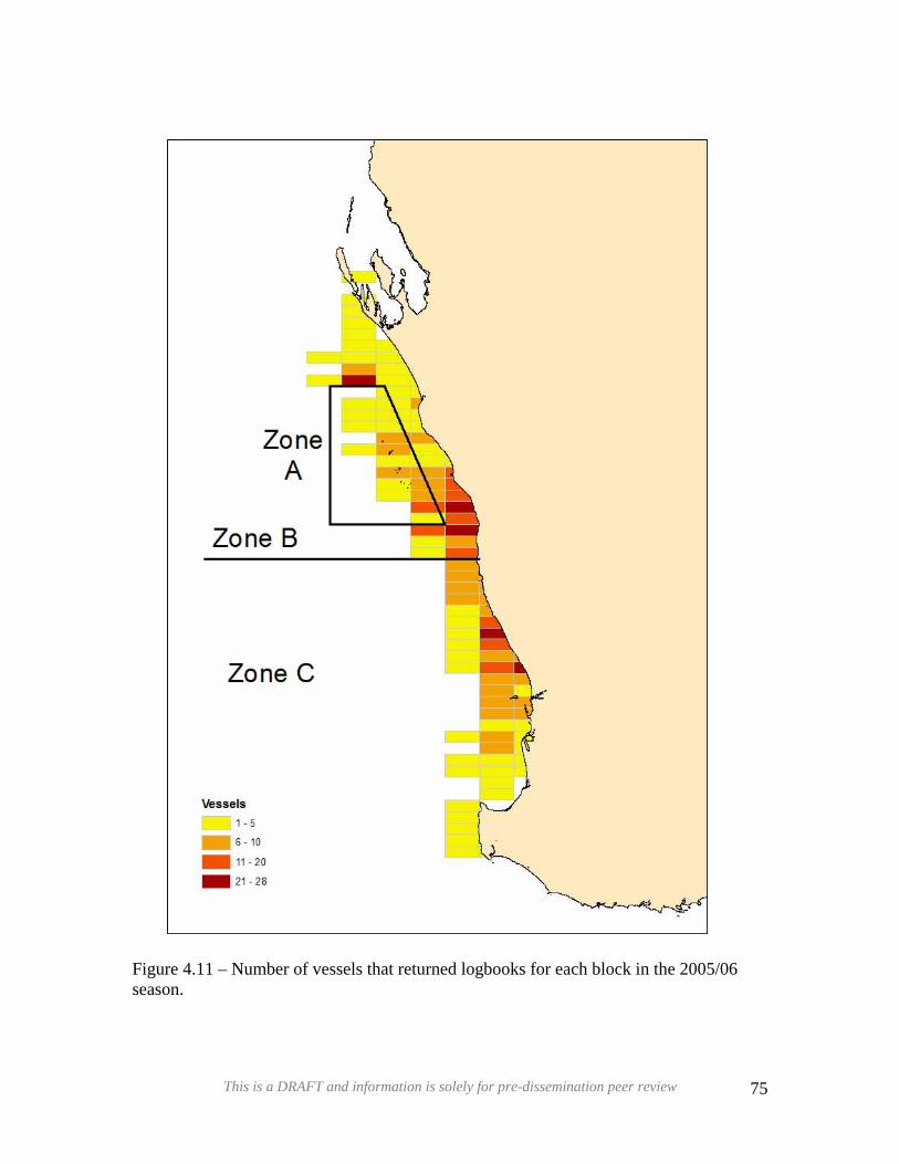
DDRRAAFFTT
Figure 4.11 – Number of vessels that returned logbooks for each block in the 2005/06 season.
This is a DRAFT and information is solely for pre-dissemination peer review 75
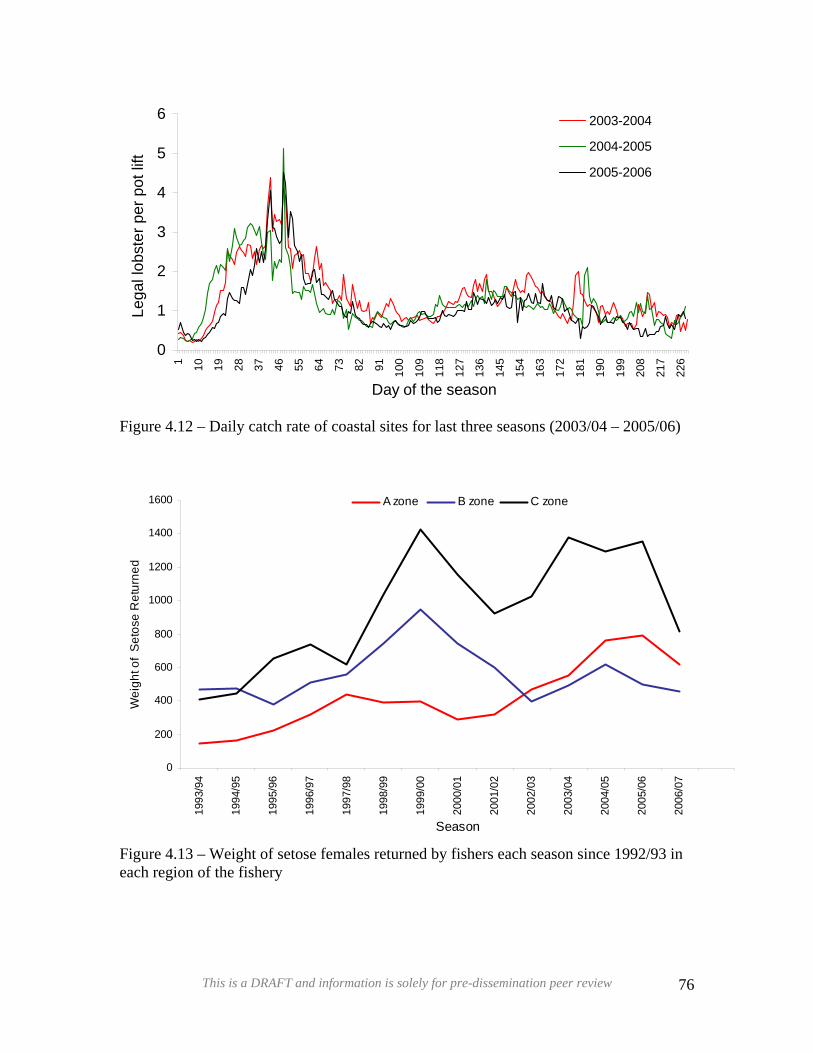
DDRRAAFFTT0
1
2
3
4
5
6
1 10 19 28 37 46 55 64 73 82 91 100
109
118
127
136
145
154
163
172
181
190
199
208
217
226
Day of the season
Lega
l lob
ster
per
pot
lift
2003-2004
2004-2005
2005-2006
Figure 4.12 – Daily catch rate of coastal sites for last three seasons (2003/04 – 2005/06)
0
200
400
600
800
1000
1200
1400
1600
1993
/94
1994
/95
1995
/96
1996
/97
1997
/98
1998
/99
1999
/00
2000
/01
2001
/02
2002
/03
2003
/04
2004
/05
2005
/06
2006
/07
Season
Wei
ght o
f S
etos
e R
etur
ned
A zone B zone C zone
Figure 4.13 – Weight of setose females returned by fishers each season since 1992/93 in each region of the fishery
This is a DRAFT and information is solely for pre-dissemination peer review 76
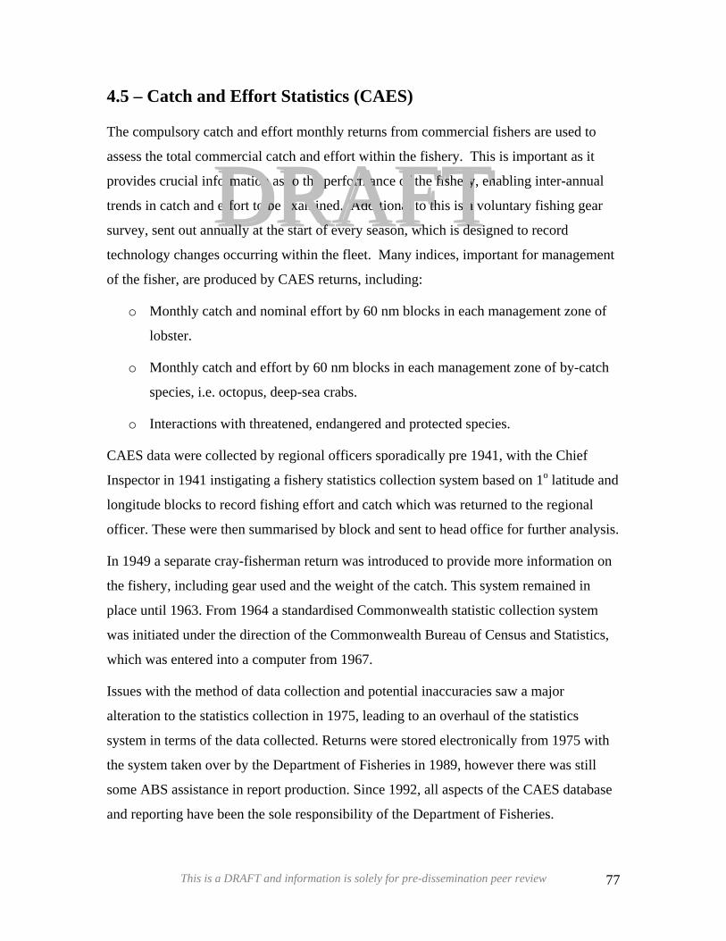
4.5 – Catch and Effort Statistics (CAES)
DRAFTThe compulsory catch and effort monthly returns from commercial fishers are used to
assess the total commercial catch and effort within the fishery. This is important as it
provides crucial information as to the performance of the fishery, enabling inter-annual
trends in catch and effort to be examined. Additional to this is a voluntary fishing gear
survey, sent out annually at the start of every season, which is designed to record
technology changes occurring within the fleet. Many indices, important for management
of the fisher, are produced by CAES returns, including:
DRAFTo Monthly catch and nominal effort by 60 nm blocks in each management zone of
lobster.
o Monthly catch and effort by 60 nm blocks in each management zone of by-catch
species, i.e. octopus, deep-sea crabs.
o Interactions with threatened, endangered and protected species.
CAES data were collected by regional officers sporadically pre 1941, with the Chief
Inspector in 1941 instigating a fishery statistics collection system based on 1o latitude and
longitude blocks to record fishing effort and catch which was returned to the regional
officer. These were then summarised by block and sent to head office for further analysis.
In 1949 a separate cray-fisherman return was introduced to provide more information on
the fishery, including gear used and the weight of the catch. This system remained in
place until 1963. From 1964 a standardised Commonwealth statistic collection system
was initiated under the direction of the Commonwealth Bureau of Census and Statistics,
which was entered into a computer from 1967.
Issues with the method of data collection and potential inaccuracies saw a major
alteration to the statistics collection in 1975, leading to an overhaul of the statistics
system in terms of the data collected. Returns were stored electronically from 1975 with
the system taken over by the Department of Fisheries in 1989, however there was still
some ABS assistance in report production. Since 1992, all aspects of the CAES database
and reporting have been the sole responsibility of the Department of Fisheries.
This is a DRAFT and information is solely for pre-dissemination peer review 77
4.5.1 – Methods
DRAFTReturns from fishers are received monthly with a deadline of 15 days after the end of the
month. Fishermen who are in arrears with their returns, are contacted every few months
by the CAES returns officer, requesting their return. Once a year a letter is sent to remind
fishers of their licensing requirements to provide a return. This ultimately provides an
annual return rate of around 98% by the end of the financial year. DRAFT
Data collected in the returns (Appendix 4) is vetted upon its receipt. Comprehensive
checks are run after data entry is completed comparing data entered to processors returns
received and to details from the Fisheries Licensing system. This includes looking at
irregularities in the number of days fished (if greater than is allowed) and, incorrect block
numbers (fishing in a block outside the zone they are licensed for). When catches from
CAES do not match that provided by lobster processors, both datasets are interrogated to
determine the inconsistencies and correct where necessary. This provides a
comprehensive, and largely accurate database as a baseline for comparing CAES data
between blocks, zones and season.
At the end of each season, a gear survey is sent to all fishers, detailing the type of gear
used, boat modifications and technology installed. This information has been collected
since 1989/90 and has been used to assess changes in fishing efficiency (Section 5.1).
This is a DRAFT and information is solely for pre-dissemination peer review 78
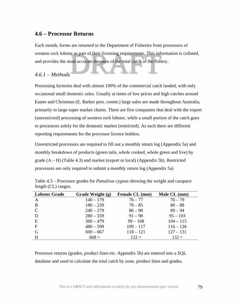
4.6 – Processor Returns
DDRRAAFFTTEach month, forms are returned to the Department of Fisheries from processors of
western rock lobster as part of their licensing requirements. This information is collated,
and provides the most accurate measure of the total catch of the fishery.
4.6.1 – Methods
Processing factories deal with almost 100% of the commercial catch landed, with only
occasional small domestic sales. Usually at times of low prices and high catches around
Easter and Christmas (E. Barker pers. comm.) large sales are made throughout Australia,
primarily to large super market chains. There are five companies that deal with the export
(unrestricted) processing of western rock lobster, while a small portion of the catch goes
to processors solely for the domestic market (restricted). As such there are different
reporting requirements for the processor licence holders.
Unrestricted processors are required to fill out a monthly return log (Appendix 5a) and
monthly breakdown of products (green tails, whole cooked, whole green and live) by
grade (A – H) (Table 4.3) and market (export or local) (Appendix 5b). Restricted
processors are only required to submit a monthly return log (Appendix 5a)
Table 4.3 – Processor grades for Panulirus cygnus showing the weight and carapace length (CL) ranges.
Lobster Grade Grade Weight (g) Female CL (mm) Male CL (mm) A 140 – 179 76 – 77 76 – 79 B 180 – 239 78 – 85 80 – 88 C 240 – 279 86 – 90 89 – 94 D 280 – 359 91 – 98 95 – 103 E 360 – 479 99 – 108 104 – 115 F 480 – 599 109 – 117 116 – 126 G 600 – 667 118 – 121 127 – 131 H 668 + 122 + 132 +
Processor returns (grades, product lines etc. Appendix 5b) are entered into a SQL
database and used to calculate the total catch by zone, product lines and grades.
This is a DRAFT and information is solely for pre-dissemination peer review 79

DDRRAAFFTTEach month a breakdown by grade product line is sent to processors. Another monthly
summery sheet is sent to District offices of the Department of Fisheries, and processors
outlining the catch in that month for three areas Fremantle (Capes to Wedge Is.), Jurien
(Green Is. to Green Head) and Geraldton (Leeman to Shark Bay). This is compared to the
catch at the same time last year and also the 10-year cumulative average to give an
indication of how the season is progressing.
This is a DRAFT and information is solely for pre-dissemination peer review 80
4.7 – Environmental Data
DDRRAAFFTTEnvironmental conditions such as water temperatures and oceanic currents greatly
influence their survival and behaviour of larval P. cygnus. As such, a number of
environmental variables is sourced by the Department of Fisheries to determine what
effects variations in climatic conditions have on the WCRLMF. Most of the data outlined
below are gathered from the Australian Government’s Bureau of Meteorology (BOM).
These data complement environmental data collected by the Department of Fisheries
during monitoring programs (see 4.1 Puerulus, 4.2 Commercial Monitoring, 4.3 IBSS,
4.4 Logbooks).
4.7.1 – Methods
Rainfall
Monthly rainfall data is collated from Bunbury, Mandurah, Rockingham, Fremantle,
Rottnest, Lancelin, Jurien, Dongara, Geraldton and Kalbarri (e.g. Bureau of Meteorology
2007). Rainfall is used as a proxy for westerly winds associated with storms crossing the
coast in winter/spring.
Sea Level
Sea level data for the west coast is obtained from BOM recordings at Hillarys
(http://www.bom.gov.au/oceanography/projects/abslmp/abslmp.shtml), and from the
National Tidal Centre for Fremantle sea level. This provides hourly sea level data as well
as data on Water Temperature, Air Temperature, Barometric Pressure, Wind Direction,
Wind Gust, Wind Speed. Archived data is available from 1992 with current data updated
monthly.
Reynolds Satellite Sea Surface Temperatures
Obtained monthly from the Commonwealth Scientific and Industrial Research
Organisation (CSIRO), the Reynolds Satellite temperatures have provided sea surface
temperatures since January 1982. Temperature is recorded for 1-degree blocks ranging
from 10o – 50o S and 90o – 130o E.
This is a DRAFT and information is solely for pre-dissemination peer review 81
Southern Oscillation Index (SOI)
DDRRAAFFTTThis is calculated from the monthly air pressure difference between Tahiti and Darwin
(BOM website). It is sourced from the BOM
(http://www.bom.gov.au/climate/current/soi2.shtml) and provides a monthly value of the
SOI, with archived values available from 1876.
The SOI reflects changes in global oceanic conditions and is usually used to denote either
El Niño or La Niña weather conditions. The change in the temperature of eastern and
central Pacific alters the strength of trade winds, rainfall patterns and also oceanic
currents. While the majority of the impact of these climatic conditions influences the
eastern seaboard of Australia (bordering the Pacific Ocean), it does impact the Leeuwin
Current off the West Australia coast. Its impact on the WRL is outlined in sections 4.1
and 5.2.
4.7.2 – Results
Southern Oscillation Index (SOI)
El Niño events (indicated by the SOI) affect Leeuwin Current strength, which can be
measured by the mean sea level at Fremantle (Pearce & Phillips 1988). The changes
between years as a result of ENSO events, has a corresponding effect of puerulus
settlement (Figure 4.14).
This is a DRAFT and information is solely for pre-dissemination peer review 82
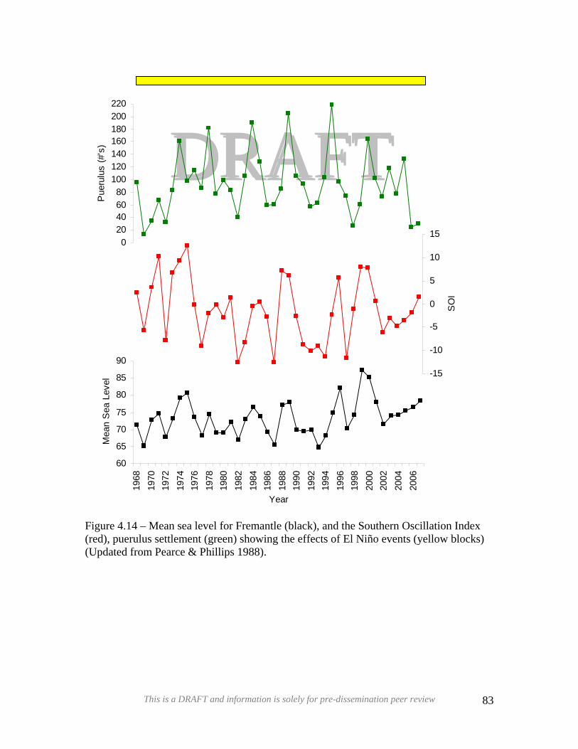
DDRRAAFFTT0
20406080
100120140160180200220
Pue
rulu
s (#
's)
-15
-10
-5
0
5
10
15
SO
I60
65
70
75
80
85
90
1968
1970
1972
1974
1976
1978
1980
1982
1984
1986
1988
1990
1992
1994
1996
1998
2000
2002
2004
2006
Year
Mea
n S
ea L
evel
Figure 4.14 – Mean sea level for Fremantle (black), and the Southern Oscillation Index (red), puerulus settlement (green) showing the effects of El Niño events (yellow blocks) (Updated from Pearce & Phillips 1988).
This is a DRAFT and information is solely for pre-dissemination peer review 83
4.8 – Recreational Fishery and Surveys
DDRRAAFFTTThe recreational rock lobster fishery primarily targets P. cygnus but also takes southern
and tropical rock lobster species using pots (traps) or by diving. Most of the fishing effort
is focused on the P. cygnus and is concentrated in the Perth metropolitan area and
Geraldton.
4.8.1 – Methods
Mail Surveys
Information on the catch, effort and fishing characteristics of recreational rock lobster
fishers has been collected in Western Australia since 1986/87 season, by an annual mail
survey of randomly selected rock lobster licence holders. Initially this survey was sent
out to one in four fishers with their licence expiry reminder letters, which usually went
out at the start of a new season, apart from the 1988/89 season when all licence holders
were sent a questionnaire.
From the 1995/96 season, a nominated quantity of licence holders has been randomly
selected at the end of the fishing season from the recreational lobster licence database.
These people have had the survey form mailed to them and have been encouraged to
return the completed questionnaire by a post-free provision, a service provided since the
initial survey in 1986/87. Questions in the survey remained relatively similar from
inception up until the 1998/99 season, where additional questions were added (Appendix
6 and 7).
Questions have been assigned to a number of categories addressing:
Participant details, such as name, address and phone number. Additional data was then
sought on the age, gender, main language spoken at home, highest education, email
address as well as the number of years they had been recreationally lobster fishing and
what licence type (rock lobster or umbrella) they used.
Fishing details, such as whether the licence holder fished that season, and if so how
(methods of fishing e.g. pot, dive or other), when they fished, and how many lobsters
(southern, western and tropical) they caught. This was initially examined as; which
This is a DRAFT and information is solely for pre-dissemination peer review 84
DDRRAAFFTTmonths they fished, when most of the fishing was conducted (weekend, weekdays, school
holidays or annual leave) and how many days were fished, broken down by fishing
method. The number of lobsters caught (also broken down by method) was recorded; as
was the number of pots they pulled each day. This was further refined by getting the
number of days fished for each month and the catch of that month, broken down by
fishing method. This has enabled a more thorough examination of the method, fishing
effort and the associated catch, to be made.
Location details of fishing effort (broken down by the methods used) were also refined in
later mail surveys. Initially the location data was quite course with the location (town
name) and postcodes used as identifiers for location, with an indication of the methods
used at that site. This was later broken down into 23 coastal regions (Figure 4.15) with
the numbers of days fished by each method in each location. The smaller blocks in the
more recent surveys have allowed for a better resolution of lobster fishing along the WA
coast.
While P. cygnus is the major targeted species, other rock lobsters taken are also surveyed
with the total number of tropical or southern lobsters caught (broken down by method)
recorded by the survey.
A lot of the more recent information gathered from the mail survey centres on the
attributes of the fishers. This includes; if they are a boat owner and the length of boat, or
if they have regular access (excluding charter boats) to a boat. Also the equipment on the
boat (B/W echo, colour echo sounder, view bucket, radar, pot winch, GPS) is recorded,
along with the pot types and the depth of potting. Depth ranges of divers are also
surveyed as well as the diving equipment used (e.g. SCUBA, snorkel, hookah, torch,
loop, hook or dive computer) and if they have dived off charter boats (no. of days and
catch). These data provide the ability to track the influence of changes in gear technology
on the ability of recreational fishers to catch lobster.
This is a DRAFT and information is solely for pre-dissemination peer review 85
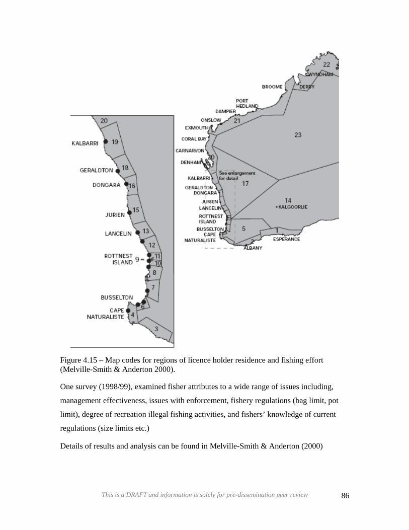
DDRRAAFFTT
Figure 4.15 – Map codes for regions of licence holder residence and fishing effort (Melville-Smith & Anderton 2000).
One survey (1998/99), examined fisher attributes to a wide range of issues including,
management effectiveness, issues with enforcement, fishery regulations (bag limit, pot
limit), degree of recreation illegal fishing activities, and fishers’ knowledge of current
regulations (size limits etc.)
Details of results and analysis can be found in Melville-Smith & Anderton (2000)
This is a DRAFT and information is solely for pre-dissemination peer review 86
Telephone Diary Surveys
DDRRAAFFTT Telephone diary surveys of recreational rock lobster fishers have been undertaken in
2000/01 and 2001/02 and have run annually from 2004/05. This initially involved 400 to
450 people being called randomly from the licence holder database, however in the
2006/07 season it has increased to 800 participants. Participants are selected randomly
from two licence types, with 50% holding a rock lobster licence and 50% hold an
umbrella licence (covering all recreational licensed fisheries).
Trained interviewers initially call the randomly selected licence holders four or more
times before they are deemed to be non-respondents. Respondents are sent a diary and
asked to fill it out for each day they go fishing for rock lobsters. Each month (or
fortnightly if they are a regular fisher), they are phoned and asked to read out from their
diary the days they went fishing and their catch (Table 4.4). Over the length of the
season 90 – 95% of fishing events are diarised.
Table 4.4 – Data recorded as part of the phone diary survey
Where and When Fishing Method Times Catch Location No. of Pots Start time Species Date Diving Finish time No. Kept / Released
Interviewers also ask additional information such as the depth of fishing, method of
diving, if it was boat or shore based, and any other comments. Location information is
pooled up into regions (see Appendix 8).
In 2005/06 a phone diary survey of registered boat owners residing on the west coast also
estimated the catch and fishing effort of western rock lobsters.
Boat Ramp Survey
The 2006/07 season saw for the first time, a boat ramp survey. This survey has monitored
the lobster catch taken by fishers from two popular boat ramps in the northern
metropolitan region (Hillarys and Ocean Reef) for 30 random days throughout December
and January. These locations were chosen as they were one of the sub regions of the
Telephone Diary survey and an enforcement officer was used as he had the power to
This is a DRAFT and information is solely for pre-dissemination peer review 87
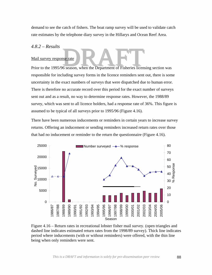
demand to see the catch of fishers. The boat ramp survey will be used to validate catch
rate estimates by the telephone diary survey in the Hillarys and Ocean Reef Area.
DDRRAAFFTT4.8.2 – Results
Mail survey response rate
Prior to the 1995/96 season, when the Department of Fisheries licensing section was
responsible for including survey forms in the licence reminders sent out, there is some
uncertainty in the exact numbers of surveys that were dispatched due to human error.
There is therefore no accurate record over this period for the exact number of surveys
sent out and as a result, no way to determine response rates. However, the 1988/89
survey, which was sent to all licence holders, had a response rate of 36%. This figure is
assumed to be typical of all surveys prior to 1995/96 (Figure 4.16).
There have been numerous inducements or reminders in certain years to increase survey
returns. Offering an inducement or sending reminders increased return rates over those
that had no inducement or reminder to the return the questionnaire (Figure 4.16).
0
5000
10000
15000
20000
25000
1986
/87
1987
/88
1988
/89
1989
/90
1990
/91
1991
/92
1992
/93
1993
/94
1994
/95
1995
/96
1996
/97
1997
/98
1998
/99
1999
/00
2000
/01
2001
/02
2002
/03
2003
/04
2004
/05
2005
/06
Season
No.
Sur
veye
d
0
10
20
30
40
50
60
70
80
% R
espo
nse
Number surveyed % response
Figure 4.16 – Return rates in recreational lobster fisher mail survey. (open triangles and dashed line indicates estimated return rates from the 1998/89 survey). Thick line indicates period where inducements (with or without reminders) were offered, with the thin line being when only reminders were sent.
This is a DRAFT and information is solely for pre-dissemination peer review 88
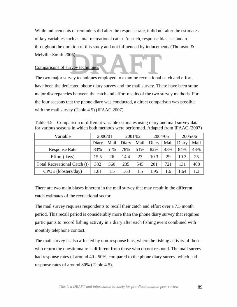
DRDRAAFFTTWhile inducements or reminders did alter the response rate, it did not alter the estimates
of key variables such as total recreational catch. As such, response bias is standard
throughout the duration of this study and not influenced by inducements (Thomson &
Melville-Smith 2005).
Comparisons of survey techniques
The two major survey techniques employed to examine recreational catch and effort,
have been the dedicated phone diary survey and the mail survey. There have been some
major discrepancies between the catch and effort results of the two survey methods. For
the four seasons that the phone diary was conducted, a direct comparison was possible
with the mail survey (Table 4.5) (IFAAC 2007).
Table 4.5 – Comparison of different variable estimates using diary and mail survey data for various seasons in which both methods were performed. Adapted from IFAAC (2007)
Variable 2000/01 2001/02 2004/05 2005/06 Diary Mail Diary Mail Diary Mail Diary Mail
Response Rate 83% 51% 78% 51% 82% 43% 84% 43% Effort (days) 15.5 26 14.4 27 10.3 29 10.3 25
Total Recreational Catch (t) 332 560 235 545 201 721 131 408 CPUE (lobsters/day) 1.81 1.5 1.63 1.5 1.95 1.6 1.64 1.3
There are two main biases inherent in the mail survey that may result in the different
catch estimates of the recreational sector.
The mail survey requires respondents to recall their catch and effort over a 7.5 month
period. This recall period is considerably more than the phone diary survey that requires
participants to record fishing activity in a diary after each fishing event combined with
monthly telephone contact.
The mail survey is also affected by non-response bias, where the fishing activity of those
who return the questionnaire is different from those who do not respond. The mail survey
had response rates of around 40 - 50%, compared to the phone diary survey, which had
response rates of around 80% (Table 4.5).
This is a DRAFT and information is solely for pre-dissemination peer review 89
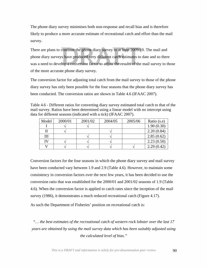
DDRRAAFFTTThere are plans to continue the phone diary survey to at least 2009/10. The mail and
phone diary surveys have produced very different catch estimates to date and so there
was a need to develop a conversion factor to adjust the results of the mail survey to those
of the more accurate phone diary survey.
The phone diary survey minimises both non-response and recall bias and is therefore
likely to produce a more accurate estimate of recreational catch and effort than the mail
survey.
The conversion factor for adjusting total catch from the mail survey to those of the phone
diary survey has only been possible for the four seasons that the phone diary survey has
been conducted. The conversion ratios are shown in Table 4.6 (IFAAC 2007).
Table 4.6 - Different ratios for converting diary survey estimated total catch to that of the mail survey. Ratios have been determined using a linear model with no intercept using data for different seasons (indicated with a tick) (IFAAC 2007).
Model 2000/01 2001/02 2004/05 2005/06 Ratio (s.e) I √ √ 1.90 (0.30) II √ √ 2.20 (0.84) III √ √ 2.85 (0.62) IV √ √ √ 2.23 (0.50) V √ √ √ √ 2.29 (0.42)
Conversion factors for the four seasons in which the phone diary survey and mail survey
have been conducted vary between 1.9 and 2.9 (Table 4.6). However, to maintain some
consistency in conversion factors over the next few years, it has been decided to use the
conversion ratio that was established for the 2000/01 and 2001/02 seasons of 1.9 (Table
4.6). When the conversion factor is applied to catch rates since the inception of the mail
survey (1986), it demonstrates a much reduced recreational catch (Figure 4.17).
As such the Department of Fisheries’ position on recreational catch is:
“… the best estimates of the recreational catch of western rock lobster over the last 17
years are obtained by using the mail survey data which has been suitably adjusted using
the calculated level of bias.”
This is a DRAFT and information is solely for pre-dissemination peer review 90
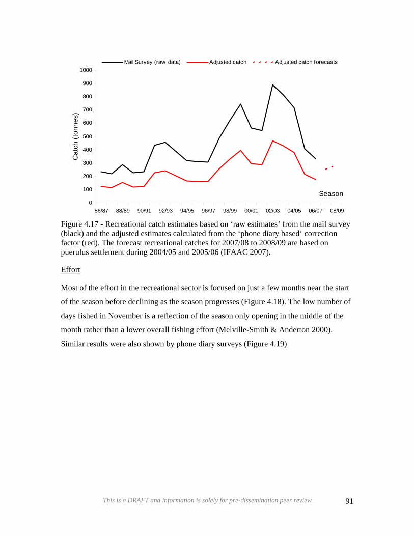
DDRRAAFFTT0
100
200
300
400
500
600
700
800
900
1000
86/87 88/89 90/91 92/93 94/95 96/97 98/99 00/01 02/03 04/05 06/07 08/09
Season
Cat
ch (t
onne
s)
Mail Survey (raw data) Adjusted catch Adjusted catch forecasts
Figure 4.17 - Recreational catch estimates based on ‘raw estimates’ from the mail survey (black) and the adjusted estimates calculated from the ‘phone diary based’ correction factor (red). The forecast recreational catches for 2007/08 to 2008/09 are based on puerulus settlement during 2004/05 and 2005/06 (IFAAC 2007).
Effort
Most of the effort in the recreational sector is focused on just a few months near the start
of the season before declining as the season progresses (Figure 4.18). The low number of
days fished in November is a reflection of the season only opening in the middle of the
month rather than a lower overall fishing effort (Melville-Smith & Anderton 2000).
Similar results were also shown by phone diary surveys (Figure 4.19)
This is a DRAFT and information is solely for pre-dissemination peer review 91
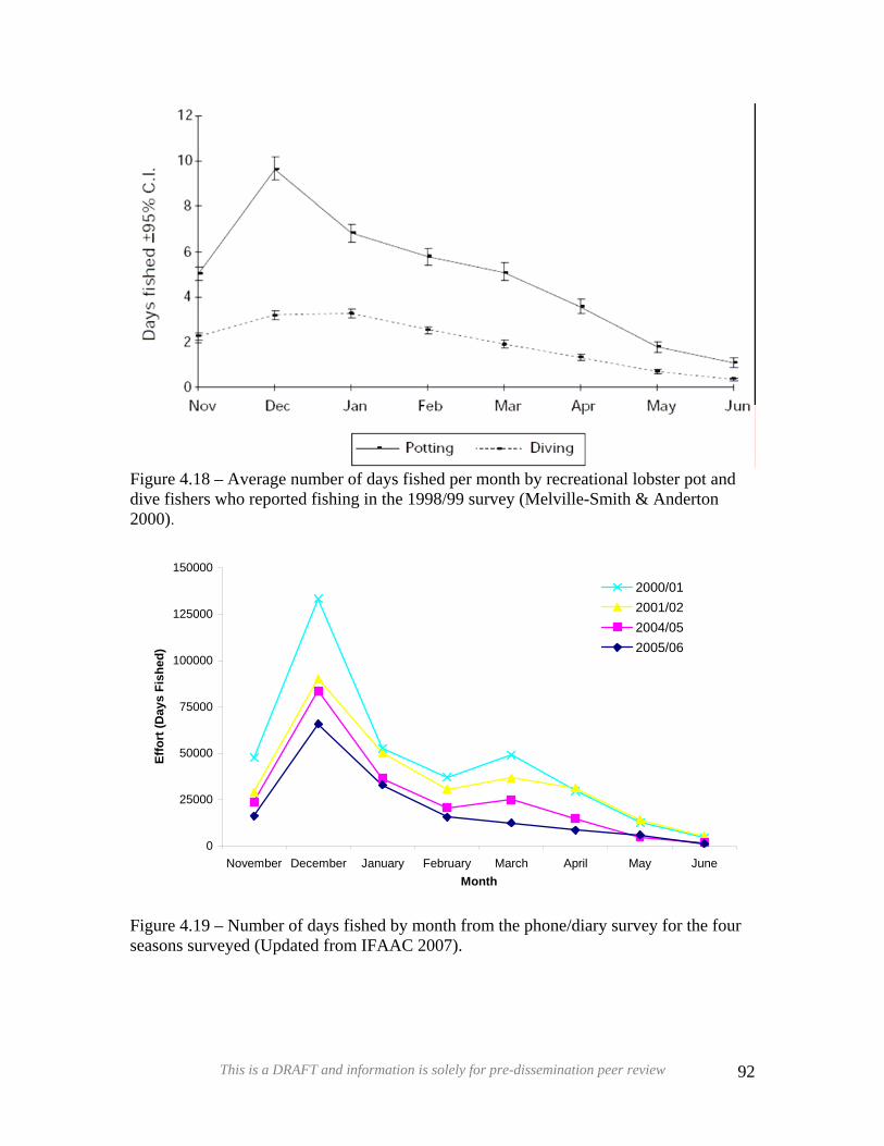
DDRRAAFFTT
Figure 4.18 – Average number of days fished per month by recreational lobster pot and dive fishers who reported fishing in the 1998/99 survey (Melville-Smith & Anderton 2000).
0
25000
50000
75000
100000
125000
150000
November December January February March April May JuneMonth
Effo
rt (D
ays
Fish
ed)
2000/012001/022004/052005/06
Figure 4.19 – Number of days fished by month from the phone/diary survey for the four seasons surveyed (Updated from IFAAC 2007).
This is a DRAFT and information is solely for pre-dissemination peer review 92
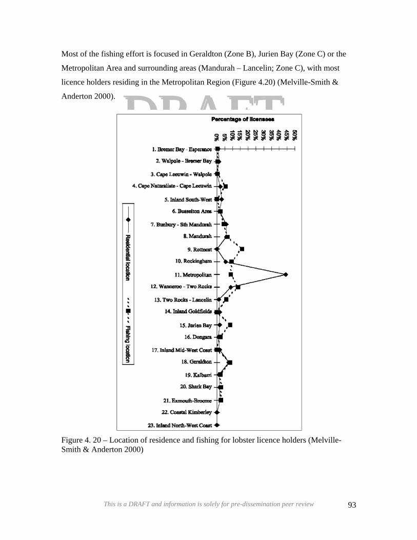
DDRRAAFFTTMost of the fishing effort is focused in Geraldton (Zone B), Jurien Bay (Zone C) or the
Metropolitan Area and surrounding areas (Mandurah – Lancelin; Zone C), with most
licence holders residing in the Metropolitan Region (Figure 4.20) (Melville-Smith &
Anderton 2000).
Figure 4. 20 – Location of residence and fishing for lobster licence holders (Melville-Smith & Anderton 2000)
This is a DRAFT and information is solely for pre-dissemination peer review 93
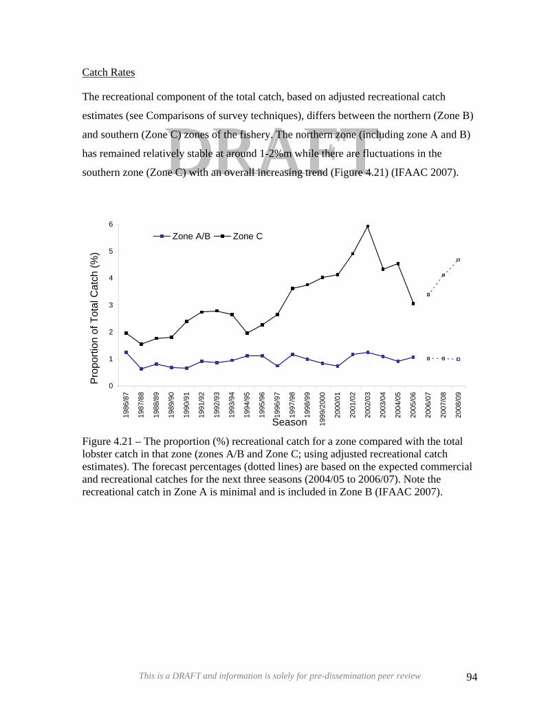
Catch Rates
DDRRAAFFTTThe recreational component of the total catch, based on adjusted recreational catch
estimates (see Comparisons of survey techniques), differs between the northern (Zone B)
and southern (Zone C) zones of the fishery. The northern zone (including zone A and B)
has remained relatively stable at around 1-2%m while there are fluctuations in the
southern zone (Zone C) with an overall increasing trend (Figure 4.21) (IFAAC 2007).
0
1
2
3
4
5
6
1986
/87
1987
/88
1988
/89
1989
/90
1990
/91
1991
/92
1992
/93
1993
/94
1994
/95
1995
/96
1996
/97
1997
/98
1998
/99
1999
/200
0
2000
/01
2001
/02
2002
/03
2003
/04
2004
/05
2005
/06
2006
/07
2007
/08
2008
/09
Season
Pro
porti
on o
f Tot
al C
atch
(%)
Zone A/B Zone C
Figure 4.21 – The proportion (%) recreational catch for a zone compared with the total lobster catch in that zone (zones A/B and Zone C; using adjusted recreational catch estimates). The forecast percentages (dotted lines) are based on the expected commercial and recreational catches for the next three seasons (2004/05 to 2006/07). Note the recreational catch in Zone A is minimal and is included in Zone B (IFAAC 2007).
This is a DRAFT and information is solely for pre-dissemination peer review 94
5 – Stock Assessment
DRAFTDRAFTIncreases in fishing efficiency (fishing power) on measures of nominal fishing effort can
lead to stock assessments being seriously flawed if these increases are not accounted for.
The first assessment of fishing power increases in this fishery were conducted by Brown
et al. (1995), who examined the impact of advances in fishing technology, such as echo
sounders and Global Positioning Systems (GPS). Subsequent estimations of fishing
efficiency have been made to account for more recent and subtle increases in fishing
efficiency and their effects on nominal effort (Section 5.2).
5.1 Fishing Efficiency
See paper by Fernandez et al. (1997) for more details.
5.1.1 – Methods
Changes in gear and technology
Brown et al. (1995) utilised several data sources to look at changes in gear and use of
improved technologies on fishing efficiency from 1971–1992. These included;
o Compulsory monthly commercial fisher returns (Section 4.5)
o Voluntary research logbooks (Section 4.4)
o Boat gear and technology interviews (Section 4.5); plus a one off interview of 50
fishers, to account for information from 1971-1989
o Compulsory monthly processor returns (Section 4.5)
The effects of gear alterations were examined for a number of seasons in each
management zone, in both shallow and deep water and during the “whites” and “reds”
parts of the fishing season.
A GLM analysis was used to compare catch rates of vessels with and without the
technology (e.g. GPS) after taking other factors that are likely to affect the catch rate into
account (e.g. month, location of fishing).
This is a DRAFT and information is solely for pre-dissemination peer review 95
Soak Time
DDRRAAFFTTA 48 – hour soak time (a pot that is left for 48 hours from the time that it is set, to the
time that it is pulled), produced an average 20% in the catch rate in deep water (>37m).
However, from 1971 – 1992 there was no significant trend in the proportion of days
fished with 48 hour soaking time. Therefore this was not included in fishing efficiency
calculations.
Pot Type
Pot type (Figure 1.3) usage did change during the period of this study, especially in the
southern zone (Zone C). Logbook data showed that beehive pots produced better catch
rates in deep water, while batten pots are more effective in shallow water. This was not
borne out in the interview data of the 50 fishers. This efficiency change from pot type
was applied to adjustments of fishing power in Zone C only, as this was the zone that
showed major change in pot type usage.
5.1.2 – Results
Pot type, along with increasing boat size, increasing bait use, use of plastic necks and
steel bottomed traps were not included in the overall calculations of fishing power, rather
they were applied separately to effort adjustments. These were combined into a
“background” efficiency increase, which was subjectively assigned as an annual 1%
increase.
Colour Sounders and GPS
Each of these technologies significantly (p < 0.05) increased efficiency by 29% in
shallow water and 53% in deep water, over the study period 1971 – 1992. This equates to
an annual increase of 0.5 – 2% increase in shallow and 1 – 4% increase in deep water.
These increases in efficiency for boats with the technology was applied to the percent of
boats each year that had the technology to determine the annual increase in fishing
efficiency for the whole fleet.
This is a DRAFT and information is solely for pre-dissemination peer review 96
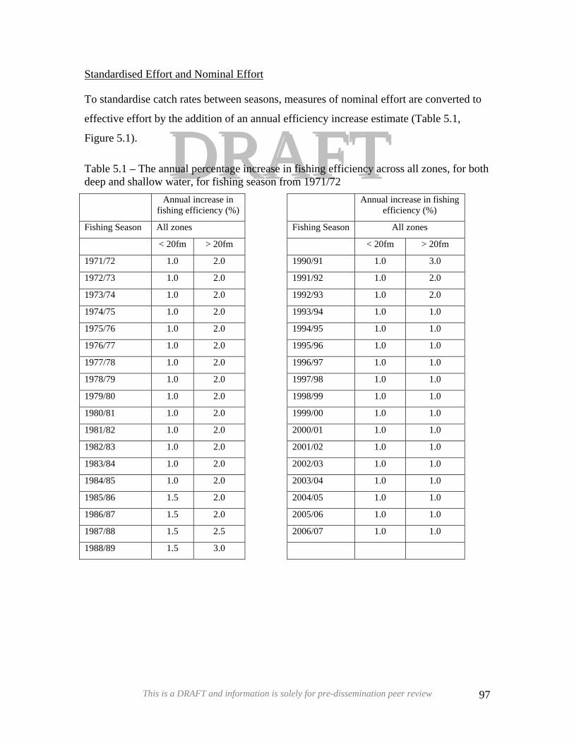
Standardised Effort and Nominal Effort
DDRRAAFFTTTo standardise catch rates between seasons, measures of nominal effort are converted to
effective effort by the addition of an annual efficiency increase estimate (Table 5.1,
Figure 5.1).
Table 5.1 – The annual percentage increase in fishing efficiency across all zones, for both deep and shallow water, for fishing season from 1971/72 Annual increase in
fishing efficiency (%) Annual increase in fishing
efficiency (%)
Fishing Season All zones Fishing Season All zones
< 20fm > 20fm < 20fm > 20fm
1971/72 1.0 2.0 1990/91 1.0 3.0
1972/73 1.0 2.0 1991/92 1.0 2.0
1973/74 1.0 2.0 1992/93 1.0 2.0
1974/75 1.0 2.0 1993/94 1.0 1.0
1975/76 1.0 2.0 1994/95 1.0 1.0
1976/77 1.0 2.0 1995/96 1.0 1.0
1977/78 1.0 2.0 1996/97 1.0 1.0
1978/79 1.0 2.0 1997/98 1.0 1.0
1979/80 1.0 2.0 1998/99 1.0 1.0
1980/81 1.0 2.0 1999/00 1.0 1.0
1981/82 1.0 2.0 2000/01 1.0 1.0
1982/83 1.0 2.0 2001/02 1.0 1.0
1983/84 1.0 2.0 2002/03 1.0 1.0
1984/85 1.0 2.0 2003/04 1.0 1.0
1985/86 1.5 2.0 2004/05 1.0 1.0
1986/87 1.5 2.0 2005/06 1.0 1.0
1987/88 1.5 2.5 2006/07 1.0 1.0
1988/89 1.5 3.0
This is a DRAFT and information is solely for pre-dissemination peer review 97
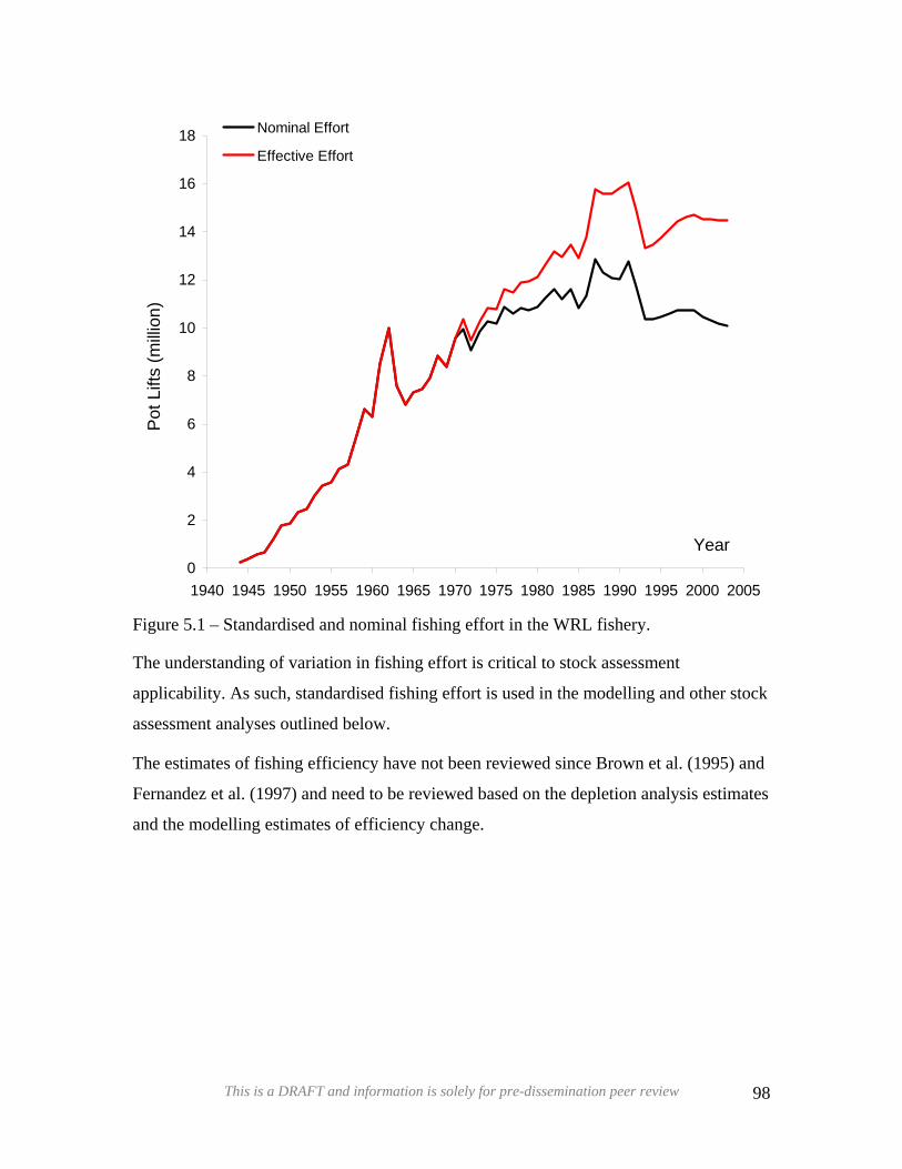
DDRRAAFFTT
0
2
4
6
8
10
12
14
16
18
1940 1945 1950 1955 1960 1965 1970 1975 1980 1985 1990 1995 2000 2005
Year
Pot
Lift
s (m
illio
n)
Nominal Effort
Effective Effort
Figure 5.1 – Standardised and nominal fishing effort in the WRL fishery.
The understanding of variation in fishing effort is critical to stock assessment
applicability. As such, standardised fishing effort is used in the modelling and other stock
assessment analyses outlined below.
The estimates of fishing efficiency have not been reviewed since Brown et al. (1995) and
Fernandez et al. (1997) and need to be reviewed based on the depletion analysis estimates
and the modelling estimates of efficiency change.
This is a DRAFT and information is solely for pre-dissemination peer review 98

5.2 – Catch Prediction
DDRRAAFFTTCatch prediction based on the level of puerulus settlement is an important tool used to
sustainably manage this fishery. It requires the use of several datasets to provide an
accurate prediction of the catch three to four years in advance. This allows sufficient
lead-time to implement any changes in management strategies to provide a sustainable
and profitable catch of WRL.
Chittleborough and Phillips (1975) were the first to describe a relationship between the
levels of puerulus settlement at the coast and variation in commercial catches. This work
soon led to the first catch predictions being produced by Morgan et al. (1982), which
were based on puerulus settlement at four locations (Seven Mile Beach, Jurien Bay, Rat
Island and Garden Island) and predicted the commercial catch of “whites” on a fishery-
wide basis. Predicting the whole seasons catch was then determined by Phillips (1986)
and Caputi and Brown (1986) using puerulus and juvenile abundances, respectively. The
current method used for predicting catch on a regional (management zone) basis for both
the whites and reds fisheries was developed by Caputi et al. (1995a) and is described in
more detail in the following section. The Department of Fisheries has recently being
modifying the technique of Caputi et al. (1995a) to incorporate finer scale variation in
puerulus settlement, juvenile growth rates, fishing efficiency and water temperature.
5.2.1 – Methods
Commercial Catch Prediction
The prediction of catches requires the combination of a number of indices namely;
puerulus settlement (Section 4.1), commercial catch and effort (Section 4.5) and
estimates of efficiency increase (Section 5.1). Catch predictions for the two coastal zones
(B and C) are produced both for the whole season and split by the two main fishing
periods, i.e. whites and reds (Section 3.3). When the sum of the predicted catches for the
whites and reds periods do not match that estimated for the whole season, the predictions
for the two fishing periods are adjusted pro rata to match the whole seasons estimate.
This is a DRAFT and information is solely for pre-dissemination peer review 99
Since the season in Zone A (Abrolhos) does not begin until the reds period, catch
predictions are produced for this period only.
DRAFTDRAFTMandPurcPurbaCatch ttt ×+×+×+= −− 43 logloglog
The general equation used to describe the relationship between puerulus settlement and
commercial catch is as follows:
where: Catch is the commercial catch (tonnes) in season t, Pur is the puerulus index 3
and 4 years before season t and Man is a management dummy variable in season t. This
dummy variable accounts for the continued impact of a management package designed to
reduce harvest rates, which was introduced in the 1993/94 fishing season (Box 2.1).
Parameter a is the intercept, b and c are measures of the density-dependent mortality
experienced by lobsters between settlement and the attainment of legal size and d
describes the relative impact of management changes. The specific factors used for catch
prediction in each management zone differ slightly:
o The Zone A catch prediction equation has traditionally used an average of
puerulus settlement at Rat Island lagged three and four years (Caputi et. al.
1995a). An improved estimate of the commercial catch in Zone A has recently
been produced by using puerulus settlement data collected at Seven Mile Beach
(Dongara), treated as two separate factors, as described in the above equation (not
as an average of the settlement three and four years previously).
o The Zone B catch prediction relationship incorporates two additional variables to
those represented in the above equation, namely a measure of effort and a second
dummy management variable. The catch prediction in this zone includes data
from the early 1970s and as such there has been an increase in nominal effort,
which has significantly, affected the catch. For predicting the whole seasons and
reds catches, the index of effort includes a fishing efficiency effect. This is not
applied to the effort index when predicting the whites catches, as these are
relatively uninfluenced by efficiency increases (Section 5.1 and Brown et. al.
1995). The second dummy variable accounts for the once off single season
This is a DRAFT and information is solely for pre-dissemination peer review 100
impact of management changes in the first season after introduction, i.e. just the
1993/94 season
DDRRAAFFTTo Originally, Zone C catch predictions were based on puerulus settlement data from
Alkimos, as this was the only location with an expansive time series of data
(Caputi et. al. 1995a). In 1997, when settlement data at other Zone C puerulus
locations has sufficient temporal coverage, these were combined with the Alkimos
data to produce a second, more spatially comprehensive index of settlement in
Zone C (Section 4.1). Recent catch predictions for this zone have been based on
same equation above, except that the dummy management variable used is the
second additional dummy variable described for Zone B and not the one described
in the above equation.
Catch prediction relationships are fitted using a log-transformed regression function in
SAS™.
Recreational Catch and Effort Prediction
The recreational catch has increased substantially since rock lobster specific licences
were first introduced in the 1986/87 fishing season. This increase, and the corresponding
increases in the recreational portion of the total catch (Figure 4.21), is of particular
interest in relation to the new management initiative of IFM (Section 1.4).
Recreational catch prediction utilises several fishery datasets including; recreational
fishery licence numbers, estimation of participation rates and catch / effort (Section 4.7),
estimation of commercial catch (Section 4.5) and, index of recruitment (Section 4.1).
Melville-Smith et al. (2001) found that a multiple regression of puerulus settlement at the
Alkimos collector (Figure 4.1) for three and four years previously and seasonal license
usage, best explained the recreational catch for that season as most of the recreational
catch is taken in the Metropolitan area.
When examined by zone, the combined parameters of puerulus settlement at Alkimos
three and four years previously and seasonal license usage in Zone C, best explained the
catch within that zone. However, for Zone B, licence usage was significant in explaining
the catch, while settlement at the collector for Zone B (Dongara) was not.
This is a DRAFT and information is solely for pre-dissemination peer review 101
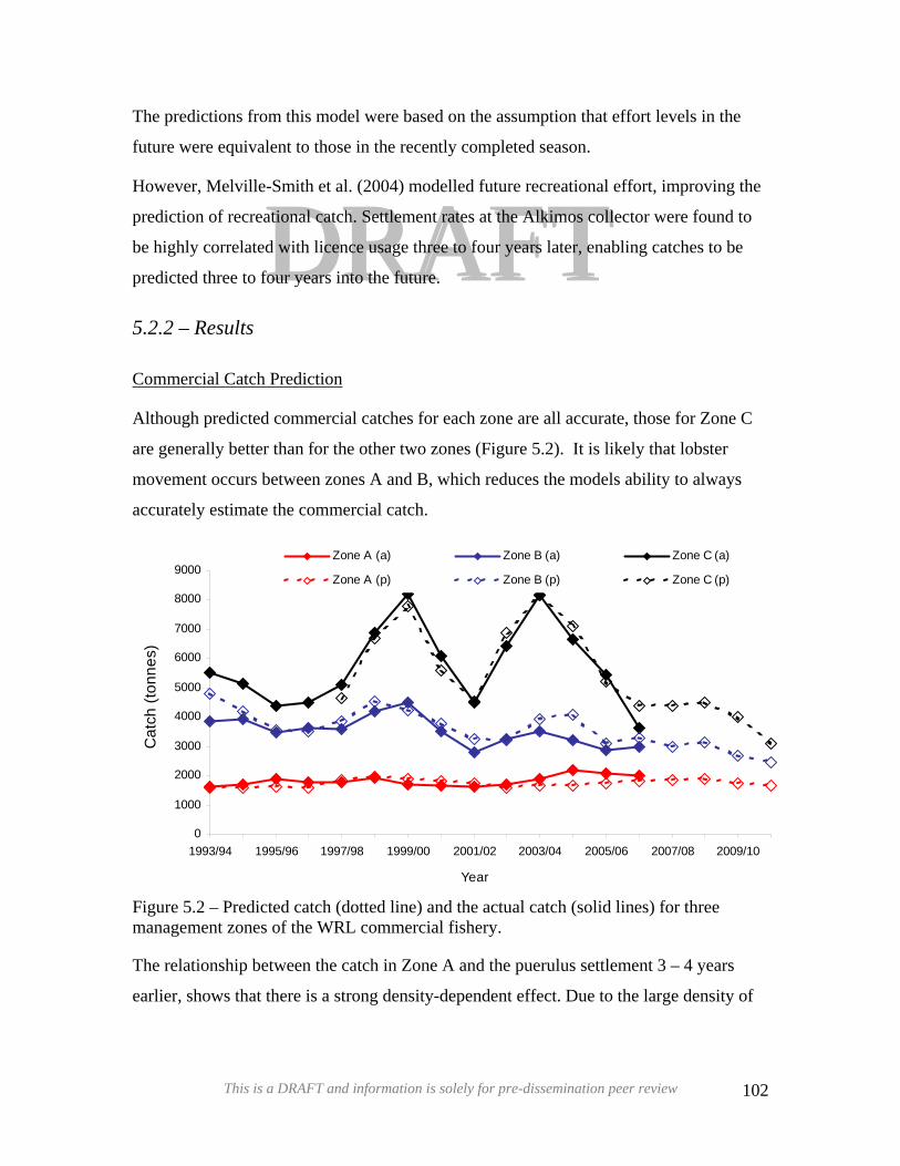
The predictions from this model were based on the assumption that effort levels in the
future were equivalent to those in the recently completed season.
DDRRAAFFTTHowever, Melville-Smith et al. (2004) modelled future recreational effort, improving the
prediction of recreational catch. Settlement rates at the Alkimos collector were found to
be highly correlated with licence usage three to four years later, enabling catches to be
predicted three to four years into the future.
5.2.2 – Results
Commercial Catch Prediction
Although predicted commercial catches for each zone are all accurate, those for Zone C
are generally better than for the other two zones (Figure 5.2). It is likely that lobster
movement occurs between zones A and B, which reduces the models ability to always
accurately estimate the commercial catch.
0
1000
2000
3000
4000
5000
6000
7000
8000
9000
1993/94 1995/96 1997/98 1999/00 2001/02 2003/04 2005/06 2007/08 2009/10
Year
Cat
ch (t
onne
s)
Zone A (a) Zone B (a) Zone C (a)
Zone A (p) Zone B (p) Zone C (p)
Figure 5.2 – Predicted catch (dotted line) and the actual catch (solid lines) for three management zones of the WRL commercial fishery.
The relationship between the catch in Zone A and the puerulus settlement 3 – 4 years
earlier, shows that there is a strong density-dependent effect. Due to the large density of
This is a DRAFT and information is solely for pre-dissemination peer review 102
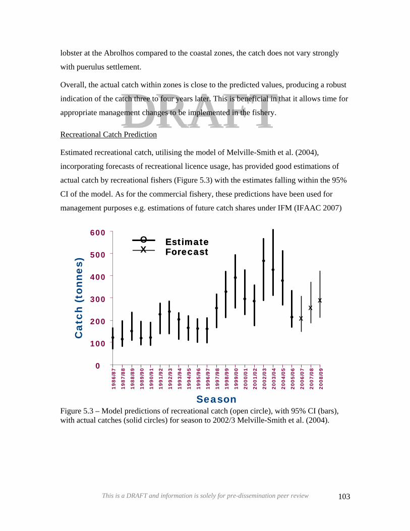
lobster at the Abrolhos compared to the coastal zones, the catch does not vary strongly
with puerulus settlement.
DDRRAAFFTTOverall, the actual catch within zones is close to the predicted values, producing a robust
indication of the catch three to four years later. This is beneficial in that it allows time for
appropriate management changes to be implemented in the fishery.
Recreational Catch Prediction
Estimated recreational catch, utilising the model of Melville-Smith et al. (2004),
incorporating forecasts of recreational licence usage, has provided good estimations of
actual catch by recreational fishers (Figure 5.3) with the estimates falling within the 95%
CI of the model. As for the commercial fishery, these predictions have been used for
management purposes e.g. estimations of future catch shares under IFM (IFAAC 2007)
XX
X
1986
/87
1987
/88
1988
/89
1989
/90
1990
/91
1991
/92
1992
/93
1993
/94
1994
/95
1995
/96
1996
/97
1997
/98
1998
/99
1999
/00
2000
/01
2001
/02
2002
/03
2003
/04
2004
/05
2005
/06
2006
/07
2007
/08
2008
/09
0
100
200
300
400
500
600
Season
Cat
ch (
tonn
es)
EstimateForecast
O EstimateX Forecast
Figure 5.3 – Model predictions of recreational catch (open circle), with 95% CI (bars), with actual catches (solid circles) for season to 2002/3 Melville-Smith et al. (2004).
This is a DRAFT and information is solely for pre-dissemination peer review 103
DDRRAAFFTTThe relationship between breeding stock and recruitment (SRR) is another important
relationship necessary for appropriate management of the fishery. Often these
relationships have proved difficult to determine, due mainly to the long larval life of
lobsters and the resulting importance of environmental conditions on recruit survival and
distribution. In fact in most cases, in order to detect a SRR the stock must first be fished
to a level whereby recruitment is significantly negatively affected. The construction of
an SRR also requires mid – long term data sets on recruitment (e.g. puerulus settlement),
abundance (Section 4.1), breeding stock (Section 4.2) and environmental measures
(Section 4.7).
5.3 – Stock Recruitment-Environment Relationship (SRR) and
Recruitment to Spawning Stock Relationship (RSR)
For complete details see Caputi et al. (1995b).
Recruitment to spawning stock relationships (RSR) describe the impact mortality (both
natural and fishing) has on the ability of recruits to replenish the spawning stock. When
combined with a SRR, the resultant model can predict equilibrium levels of stock and
recruitment for different levels of effort, which is invaluable in the management of many
fisheries.
5.3.1 – Methods
An SRR and a RSR were determined for each of the three management zones. Puerulus
settlement indices were used for each zone, with Rat Island settlement used for Zone A,
Seven Mile Beach used for Zone B and Alkimos for Zone C (Section 4.1). The northern
and southern coastal fishery dependant BSI (Section 4.2) was used as measures of the
breeding stock in those two areas. Since no direct breeding stock index was available for
the Abrolhos Islands, and the majority of the catch in this location is of a mature size, the
annual commercial catch was used as a measure of the breeding stock for Zone A.
Two main environmental measures were employed for use in the SRRs, i.e. Leeuwin
Current strength, as measured by the mean sea level at Fremantle and mean monthly
rainfall at five locations in the southern part of the fishery over two periods (July –
This is a DRAFT and information is solely for pre-dissemination peer review 104
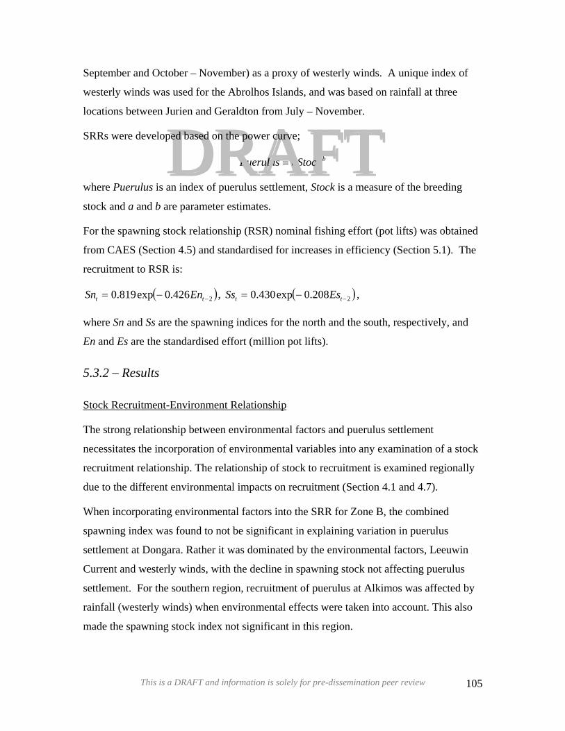
DDRAFTTbaStockPuerulus =RAFSeptember and October – November) as a proxy of westerly winds. A unique index of
westerly winds was used for the Abrolhos Islands, and was based on rainfall at three
locations between Jurien and Geraldton from July – November.
SRRs were developed based on the power curve;
where Puerulus is an index of puerulus settlement, Stock is a measure of the breeding
stock and a and b are parameter estimates.
For the spawning stock relationship (RSR) nominal fishing effort (pot lifts) was obtained
from CAES (Section 4.5) and standardised for increases in efficiency (Section 5.1). The
recruitment to RSR is:
( )2426.0exp819.0 −−= tt EnSn , ( )2208.0exp430.0 −−= tt EsSs ,
where Sn and Ss are the spawning indices for the north and the south, respectively, and
En and Es are the standardised effort (million pot lifts).
5.3.2 – Results
Stock Recruitment-Environment Relationship
The strong relationship between environmental factors and puerulus settlement
necessitates the incorporation of environmental variables into any examination of a stock
recruitment relationship. The relationship of stock to recruitment is examined regionally
due to the different environmental impacts on recruitment (Section 4.1 and 4.7).
When incorporating environmental factors into the SRR for Zone B, the combined
spawning index was found to not be significant in explaining variation in puerulus
settlement at Dongara. Rather it was dominated by the environmental factors, Leeuwin
Current and westerly winds, with the decline in spawning stock not affecting puerulus
settlement. For the southern region, recruitment of puerulus at Alkimos was affected by
rainfall (westerly winds) when environmental effects were taken into account. This also
made the spawning stock index not significant in this region.
This is a DRAFT and information is solely for pre-dissemination peer review 105
DDRRAAFFHowever, at the Abrolhos Islands, the spawning stock, when combined with rainfall in
northern locations, was significant in explaining recruitment at the Abrolhos Islands. This
may make the Abrolhos Islands more susceptible to reductions in spawning stock, as
environmental factors do not dominate in the same way that they do in the coastal
locations (for more detail see Caputi et al. 1995b). TTRecruitment to Spawning Relationship
Examination of recruits into the spawning stock showed that fishing effort two years prior
to spawning, when lobsters recruit into the fishery, significantly affected the spawning
index, but puerulus abundance was not significant. This indicates that the fishing effort
on recruits reaching legal size is the main factor affecting the abundance of the spawning
stock. In all regions of this fishery, fishing pressure is currently at such levels that good
recruitment years do not translate into good spawning stock (for more detail see Caputi et
al. 1995b).
5.3.3 –Discussion
As the spawning stock has generally increased since this analysis has been undertaken,
the spawning stock is unlikely to have become a significant factor affecting puerulus
settlement. Therefore the focus in more recent years has been to update the environment-
puerulus relationship (Section 4.7) to understand the factors affecting puerulus
settlement.
However, it would be useful to update both of these relationships, particularly the RSR,
to understand the effect of changes in fishing effort and other management measures (e.g.
setose rule) have had on these relationships.
This is a DRAFT and information is solely for pre-dissemination peer review 106
5.4 – Depletion Analysis
DDRRAAFFTTDepletion methods have the potential to provide an alternative approach for assessing
stocks that are subject to unknown (efficiency) biases. They do this because they can
estimate this efficiency changes while also producing estimates of the harvest rate and an
index of abundance. Depletion-based methodology (Delury 1947, Leslie & Davis 1939)
was applied to the western rock lobster fishery from 1984 – 2003, to determine the
applicability of the method (Wright et al. 2006)
The basic DeLury method for estimating catchability and population size is based on a
relationship between the decline in CPUE and the cumulative catch that is removed from
the fishery (Ricker 1975). The slope of this (linear) relationship provides an estimate of
the catchability of the unit of fishing. The extrapolation of the relationship down to the
point where the CPUE is zero (Ricker 1975) provides an estimate of the population size.
Assessment indices generated by this analysis include annual trends in harvest rate, total
population estimate and residual biomass after the completion of fishing, and catchability
of the fishing effort that reflects the efficiency of effort applied by the fleet.
The non-migratory phase “reds” provides an opportunity for using the depletion
assessment as it generally satisfies the key assumptions. It has been undertaken using the
monthly catch and effort of each of the three zones during the months of March – June
for each fishing season since 1983/84. The migratory phase of the fishery is not suitable
for a depletion analysis as migration of some of the lobsters from shallow water to deep
water changes their catchability compared with the non-migrating lobsters.
5.4.1 - Methods
The depletion model is based on the assumption that CPUE changes reflect changes in
abundance and not environmental (Morgan 1974 , Srisurichan 2001, Srisurichan et al.
2005) or biological effects on catchability. The assessment does not produce reliable
results unless any catchability changes are accounted for by standardising the CPUE for
environmental and biological changes between months and years. Other complicating
factors include the timing of the February moult and its impact on the availability of
recruiting lobsters during March and annual variation in the spatial distribution of effort.
This is a DRAFT and information is solely for pre-dissemination peer review 107
DDRRAAFFTTIf the moult is late in any year the assumption of no recruitment during the period is not
met and this needs to be taken into account for that year’s depletion assessment. The
depletion analysis also assumes that effort remains relatively constant. However, annual
variations in lobster abundance within a management zone, especially Zone C, can cause
effort to contract and expand. The exact influence this has on the depletion analysis
needs to be investigated.
The classical DeLury depletion model has:
Ct/Ft = q Bt Eq. 5.4.1
where Bt is the biomass present at time t. For our estimation procedure we use a
reformulation of this model based on the following quantities: Ct = catch in month t in
tones; Ft = effort in month t in thousands of pot lifts; Bt = average biomass in month t;
q = catchability standardised for temperature and swell; B0 = total biomass in zone at start
of harvest (March); K = scale factor that correctly sets the coefficient of variation of the
monthly catches in this model and through this the standard errors in our parameter
estimates. The method for determining this parameter is considered presently in the
assumptions section.
Taking Bt =B0 + 0.5Ct – ∑=
t
iiC
1 Eq. 5.4.2
where the index i ranges over the time period defined, our model becomes:
Ct has the probability distribution
K Poisson (q Ft Bt / K ) Eq. 5.4.3
for month t = 1,2,3,4 (i.e. March –June).
In our initial modelling, the parameters B0 and q in Equations Eq. 5.4.2 and Eq. 5.4.3
were estimated by Maximum Likelihood and by comparing the predicted and observed
catch, first by using Fortran code (Numerical Recipes) and later using an Excel
spreadsheet (Solver). However, since the model could be naturally formulated in a
Bayesian framework, we were able to avoid optimisation fine-tuning problems (and more
importantly automatically obtain standard errors) by using Bayesian estimation via the
This is a DRAFT and information is solely for pre-dissemination peer review 108
DDRRAAFFTTFor each zones of the fishery, there were 20 depletions to be estimated during the period
1984-2003. For this production phase, the estimation was performed by the program
BUGS 0.6 (Spiegelhalter et al. 1996) running in batch mode.
Markov Chain Monte Carlo (MCMC) method. The rationale for using the MCMC
method was the automatic estimation of standard errors for our parameters, regardless of
the model type and complexity.
The parameter estimates were effectively the medians of a sample of 10 000 from the
simulated posterior distributions based on over-dispersed priors. The priors were
exponential distributions with large means. The standard errors for the estimates were
the observed standard deviations of the posterior distributions of the parameters. The
sample of 10 000 consecutive simulated values used for our estimates followed a “burn-
in” period of 20 000 samples. Following this burn-in we confirmed that the convergence
diagnostics were comfortably within required ranges. The parameter estimates obtained,
and their standard errors and coefficients of variation, are presented in the results section
for the years 2001-03, to illustrate typical values and their precision.
The MCMC methodology results in the converged Markov chains above simulating
“depletion” lines with parameter values from their respective prior distributions. The
intersection of these depletion lines with the vertical ordinate through each catch rate
(CPUE) point realises a conditional distribution. When there is a (linear) depletion, a plot
of the medians of these conditional distributions against the cumulative catch is a straight
line. In Figure 5.4, within each year, the horizontal scale uses the cumulative catch from
March on as a fraction of the total March–June catch. For Zone A, there is a very close
agreement between the actual and Bayesian estimates of mean CPUE for each month.
Zone C depletions also show close agreement.
This is a DRAFT and information is solely for pre-dissemination peer review 109
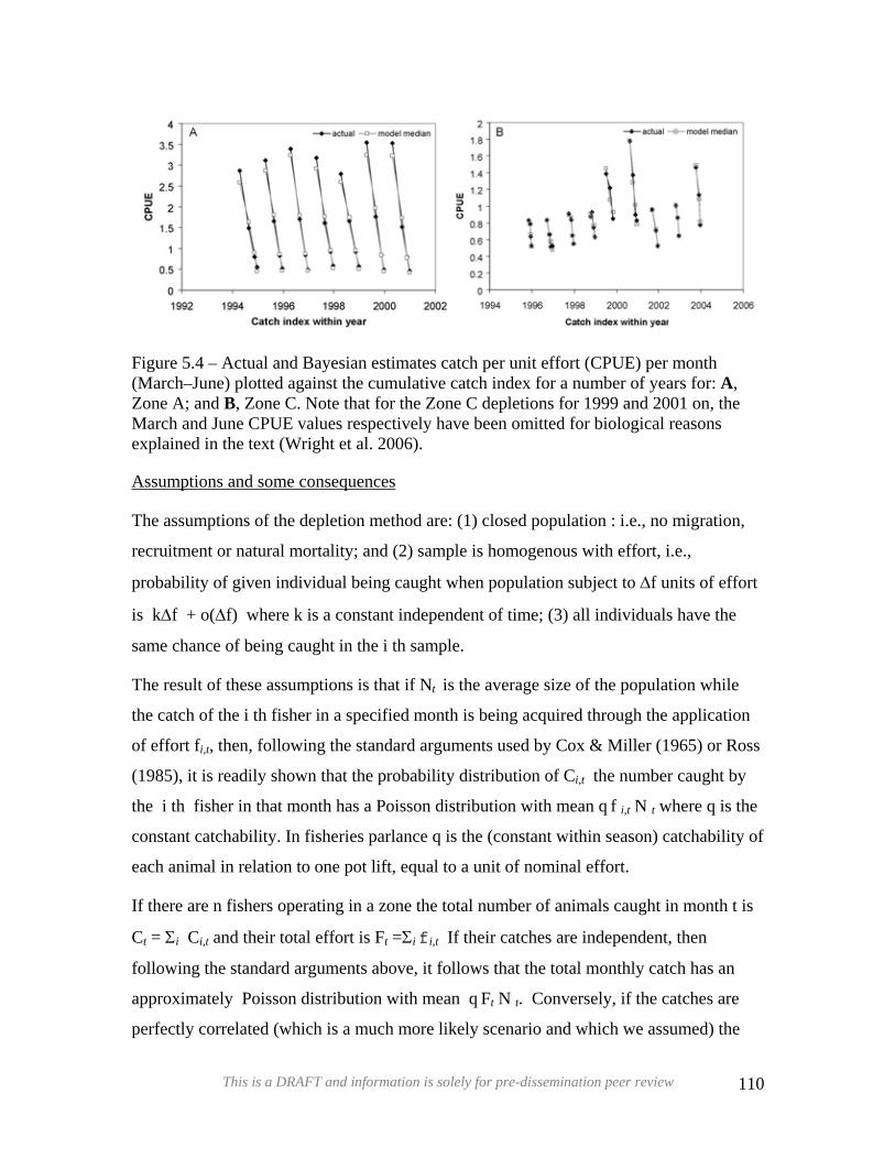
DDRRAAFFTT
Figure 5.4 – Actual and Bayesian estimates catch per unit effort (CPUE) per month (March–June) plotted against the cumulative catch index for a number of years for: A, Zone A; and B, Zone C. Note that for the Zone C depletions for 1999 and 2001 on, the March and June CPUE values respectively have been omitted for biological reasons explained in the text (Wright et al. 2006).
Assumptions and some consequences
The assumptions of the depletion method are: (1) closed population : i.e., no migration,
recruitment or natural mortality; and (2) sample is homogenous with effort, i.e.,
probability of given individual being caught when population subject to ∆f units of effort
is k∆f + o(∆f) where k is a constant independent of time; (3) all individuals have the
same chance of being caught in the i th sample.
The result of these assumptions is that if Nt is the average size of the population while
the catch of the i th fisher in a specified month is being acquired through the application
of effort fi,t, then, following the standard arguments used by Cox & Miller (1965) or Ross
(1985), it is readily shown that the probability distribution of Ci,t the number caught by
the i th fisher in that month has a Poisson distribution with mean q f i,t N t where q is the
constant catchability. In fisheries parlance q is the (constant within season) catchability of
each animal in relation to one pot lift, equal to a unit of nominal effort.
If there are n fishers operating in a zone the total number of animals caught in month t is
Ct = Σi Ci,t and their total effort is Ft =Σi fi,t If their catches are independent, then
following the standard arguments above, it follows that the total monthly catch has an
approximately Poisson distribution with mean q Ft N t. Conversely, if the catches are
perfectly correlated (which is a much more likely scenario and which we assumed) the
This is a DRAFT and information is solely for pre-dissemination peer review 110
DDRRAAFFTTtotal monthly number of animals caught is approximately distributed as n times Poisson
with mean q Ft N t /n. The mean of this Poisson distribution is the average monthly catch
of animals per fisher which is between 5000 in Zone C and 10 000 in Zone A. The
respective distributions have coefficients of variation ranging between 1.4% and 1%,
respectively.
To consider the catch for biomass (tonnes) it can be readily shown that with a conversion
rate of 2000 animals per tonne, the monthly zone catch in tonnes will be distributed as K
times a Poisson distribution with parameter equal to average monthly catch (tonnes)
divided by K, where K is determined so that the coefficient of variation of the biomass
distribution is equal to that for the distribution of animals described above. In Zone C the
average monthly catch is 552 t so that K = 1/9, in Zone B the average monthly catch is
370 t so K = 1/16, whereas in Zone A the average monthly catch is 480 t so that K = 1/21.
These scale factors have an important influence on the standard errors of our parameter
estimates, but do not affect the median values.
When the t-th sample (zone monthly catch) represents a significant proportion of the
remaining population, the value of Nt is taken to be the average value of the population
during the sampling period. This improvement owing to Braaten (1969) was endorsed by
Ricker (1975). Our estimation process includes this feature in both its frequentist and
Bayesian versions.
Environmental influence on catchability
We consider three main environmental influences on catchability: temperature, swell and
moon phase.
The swell index in the zone is the average throughout the month of swell levels recorded
in fishers daily logbooks (Section 4.4) on the scale: (0=none,10=Low, 20=Moderate,
30=High). The average monthly water temperature is determined by fisheries staff in
conjunction with other local monitoring activities (Section 4.2 and 4.7).
We derived corrections for the impact on catchability of: temperature alone (with all
other environmental variables held constant); swell alone (with all other environmental
This is a DRAFT and information is solely for pre-dissemination peer review 111
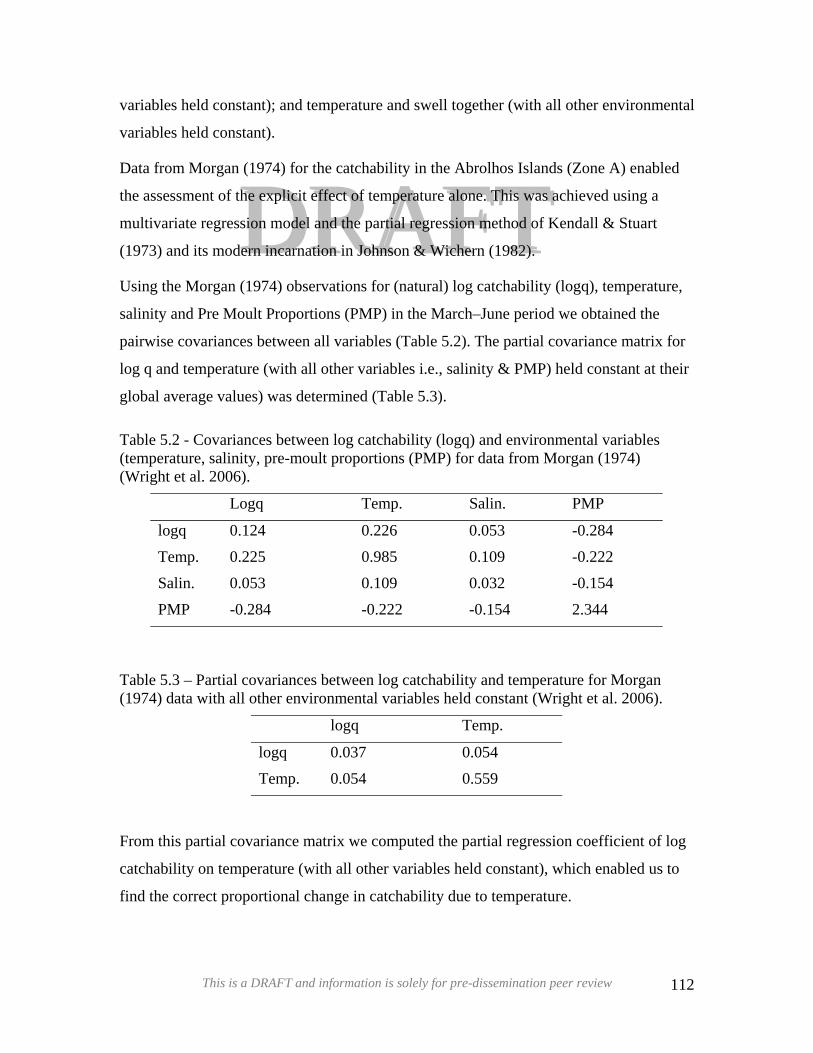
variables held constant); and temperature and swell together (with all other environmental
variables held constant).
DDRRAAFFTTData from Morgan (1974) for the catchability in the Abrolhos Islands (Zone A) enabled
the assessment of the explicit effect of temperature alone. This was achieved using a
multivariate regression model and the partial regression method of Kendall & Stuart
(1973) and its modern incarnation in Johnson & Wichern (1982).
Using the Morgan (1974) observations for (natural) log catchability (logq), temperature,
salinity and Pre Moult Proportions (PMP) in the March–June period we obtained the
pairwise covariances between all variables (Table 5.2). The partial covariance matrix for
log q and temperature (with all other variables i.e., salinity & PMP) held constant at their
global average values) was determined (Table 5.3).
Table 5.2 - Covariances between log catchability (logq) and environmental variables (temperature, salinity, pre-moult proportions (PMP) for data from Morgan (1974) (Wright et al. 2006).
Logq Temp. Salin. PMP
logq 0.124 0.226 0.053 -0.284
Temp. 0.225 0.985 0.109 -0.222
Salin. 0.053 0.109 0.032 -0.154
PMP -0.284 -0.222 -0.154 2.344
Table 5.3 – Partial covariances between log catchability and temperature for Morgan (1974) data with all other environmental variables held constant (Wright et al. 2006).
logq Temp.
logq 0.037 0.054
Temp. 0.054 0.559
From this partial covariance matrix we computed the partial regression coefficient of log
catchability on temperature (with all other variables held constant), which enabled us to
find the correct proportional change in catchability due to temperature.
This is a DRAFT and information is solely for pre-dissemination peer review 112
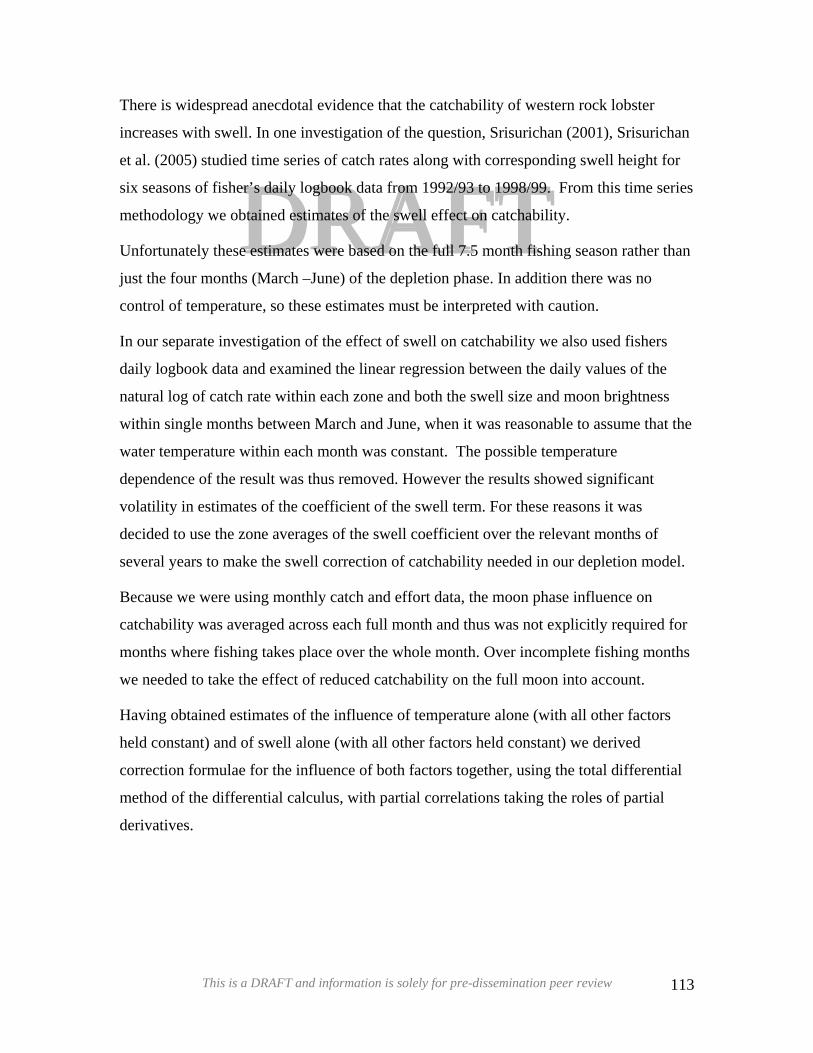
DDRRAAFFTTThere is widespread anecdotal evidence that the catchability of western rock lobster
increases with swell. In one investigation of the question, Srisurichan (2001), Srisurichan
et al. (2005) studied time series of catch rates along with corresponding swell height for
six seasons of fisher’s daily logbook data from 1992/93 to 1998/99. From this time series
methodology we obtained estimates of the swell effect on catchability.
Unfortunately these estimates were based on the full 7.5 month fishing season rather than
just the four months (March –June) of the depletion phase. In addition there was no
control of temperature, so these estimates must be interpreted with caution.
In our separate investigation of the effect of swell on catchability we also used fishers
daily logbook data and examined the linear regression between the daily values of the
natural log of catch rate within each zone and both the swell size and moon brightness
within single months between March and June, when it was reasonable to assume that the
water temperature within each month was constant. The possible temperature
dependence of the result was thus removed. However the results showed significant
volatility in estimates of the coefficient of the swell term. For these reasons it was
decided to use the zone averages of the swell coefficient over the relevant months of
several years to make the swell correction of catchability needed in our depletion model.
Because we were using monthly catch and effort data, the moon phase influence on
catchability was averaged across each full month and thus was not explicitly required for
months where fishing takes place over the whole month. Over incomplete fishing months
we needed to take the effect of reduced catchability on the full moon into account.
Having obtained estimates of the influence of temperature alone (with all other factors
held constant) and of swell alone (with all other factors held constant) we derived
correction formulae for the influence of both factors together, using the total differential
method of the differential calculus, with partial correlations taking the roles of partial
derivatives.
This is a DRAFT and information is solely for pre-dissemination peer review 113
Optimal Estimation of Underlying Trend.
DDRRAAFFTTCentred Moving Average Estimate
When underlying process has constant variance of its terms and a linear trend the centred
moving average is an efficient estimate from an error variance standpoint, although the
latest estimate is lagged by half the span of the averaging. This lag can create problems in
real time process control in certain systems. Use of a three-point moving average is a
reasonable compromise between timeliness and precision when incremental control
measures are employed.
Optimal Combinations of Estimators
If E1 and E2 are independent unbiased estimates of a parameter, the minimum variance
unbiased estimate of that parameter is a weighted mean of E1 and E2 with weights
totalling 1 and inversely proportional to the respective estimator variances.
In symbols, if E* is the minimum variance combination of the two estimators we have
E* = w1.E1 + w2.E2 Eq. 5.4.4
Where w1= (1/varE1)/(1/VarE1 + 1/VarE2) Eq. 5.4.5
and
w2 = (1/varE2)/(1/VarE1 + 1/VarE2). Eq. 5.4.6
It is readily verified that E* is an unbiased estimator because w1+w2 =1 and these values
of w1,w2 lead to a minimum point for Variance(E*). These results generalise naturally to
three or more estimators.
Weighted Moving Average Smoothing of time series data.
One favourable aspect of our WinBugs estimation of parameters is the availability of
error variances for our parameter estimates, which makes it possible to combine the
moving average approach with the minimum estimator variance methodology.
Suppose our time series is written as (X t, t =1..n). The smoothed time series is
(X* t, t =2,n-1) where
This is a DRAFT and information is solely for pre-dissemination peer review 114
X* t = w(t-1).X t-1+w(t).X t+w(t+1). X t+1 Eq. 5.4.7
In which
DDRRAAFFTTIt can be shown that in the presence of autocorrelation the trend estimator X*
w(t)=1/var(X t)/(1/var(X t-1)+1/var(X t)+1/Var(X t+1 )). Eq. 5.4.8
t has almost
as small a variance as that when there is no autocorrelation, and thus is very efficient.
Cycles in moving average smoothed series.
In our early attempts to smooth our series of estimates we did encounter some cycles in
the moving average smoothed estimates. This problem has largely disappeared when we
use the weighted smoother because the large outlying values that caused the problem
usually had large standard errors and so were downgraded by the weighting process.
However the possibility still exists for the appearance of cycles in the smoothed series
due to the operation of the Yule-Slutsky effect identified in the 1930s as an artefact of
moving average smoothing.
Environmentally Corrected Catchability
Implementing the temperature and swell corrections determined provided the following
temperature and swell correction formulae for our three Zones:
Zone A: q1= q 0 . exp( 0.097 .∆T + 0.010 . ∆S) Eq. 5.4.9
Zone B: q1= q 0 . exp( 0.080 .∆T + 0.010 . ∆S) Eq. 5.4.10
Zone C: q1= q 0 . exp( 0.080 .∆T + 0.012 .∆S) Eq. 5.4.11
where ∆T = temperature increment above 21.4oC and ∆S = swell index increment above
9.5.
Since the moon brightness cycle has a period of c. 30 days, the average value is the same
every month. Thus there is generally no need for explicit corrections for whole months.
However, the combination of full moon and cold period in June may result in fishers
ceasing fishing early. This can result in an elevated catch rate for the influential final
catch, which may be reduced by some animals beginning to moult. Also the March catch
This is a DRAFT and information is solely for pre-dissemination peer review 115
at the Abrolhos, which covers a 17-day period, is at the start (and thus less influential
part) of the depletion curve (Ricker 1975).
DDRRAAFFTTDiagnostics for Depletion Model Validity
The graph of CPUE against cumulative catch during each season, the depletion curve,
was used to monitor our depletion estimates to ensure model assumptions remained
appropriate.
Depletion based estimates for fishery harvest
Harvest rate is defined as the relative proportion of the exploited stock that is removed by
the fishery, e.g., for the reds part of the fishery (March–June):
Harvest reds = (catch reds)/(Catch reds + Residual biomass in June) Eq. 5.4.12
For Zone A this definition covers the harvest of the entire season, but for Zones B and C
this is effectively the harvest of legal-size rock lobsters over part of the season.
Depletion based estimates for residual biomass
Because the residual biomass estimated by our depletion procedure is always the legally-
exploitable biomass of the day, the present legal biomass can only be compared with the
pre-1993 biomass if we correct for the change in the definition in the legal biomass that
occurred since the 1993/94 season. This change resulted in setose females and those
above the maximum female size that would have been part of the catch before the
1993/94 season being returned to the sea and hence should be added to the residual
biomass. An estimate of the setose and females above the maximum size that were
returned to the sea was based on data collected from fishers’ daily logbooks. The estimate
of the June residual biomass based on the depletion analysis was adjusted to obtain an
estimate of the residual biomass in the pre-1993 definition of legal biomass and hence the
harvest rate based on the pre-1993 terms. These can be defined as:
Residual biomass pre 1993 = June residual biomass + mature female biomass returned
Harvest pre 1993 reds = (Catch reds)/(Catch reds + Residual biomass pre 1993).
This is a DRAFT and information is solely for pre-dissemination peer review 116
The estimate of the harvest for the whole season was obtained by adding the whites catch
during the first part of the season to the reds catch and using the total catch as follows:
DRRAAFFTTD5.4.2 – Results
Harvest pre 1993 total = (Catch total)/(Catch total + Residual biomass pre 1993)
The depletion analysis provided estimates of the residual biomass of the legally exploited
biomass at the end of the fishing season in June, the catchability and the harvest rate
during March–June (reds period) for each of the three zones of the fishery. However the
definition of the legally exploited biomass has changed since 1993/94 as mature females
with setose pleopods and females above a certain size were required to be returned to the
sea. Before 1993/94 only ovigerous females were required to be returned to sea. It is
therefore important to note that the harvest rate reported here is for the whole season and
it accounts for the 1993/94 management changes (Box 2.1) and the catch during the
migrating whites part of the fishery.
Harvest trends in Zone A
Residual biomass in Zone A remained relatively constant, before steadily increasing after
the introduction of management changes in 1993/94, with current estimates (2004/05)
being at their highest levels (~600 t). Harvest rates also began to change in 1993/94,
progressively rising to ~90% in the early 2000s. In recent seasons, the harvest rate has
declined slightly to ~ 85%. Catchability, which provides an indication of changes in
fishing efficiency, jumped markedly with the reduction of pots fishing in this zone with
the implementation of pot reductions in 1993/94. This may reflect the effects of pot
saturation. Since this rise, fishing efficiency has remained relatively constant (Figure
5.5).
Harvest trends in Zone B
Residual biomass in Zone B has been progressively declining since a peak in 1995/96. In
the past three seasons the residual biomass has ranged between 700 and 800 t. The
harvest rate in this zone has progressively increased, apart from a small decline as a result
of the 1993/94 management changes, since the mid 1980s. This increase has recently
This is a DRAFT and information is solely for pre-dissemination peer review 117
DDRRAAFFTTlevelled off, with currently estimates being around 80%. Catchability has increased
rapidly since 1995/96 (Figure 5.6). While fishing efficiency affects catchability, the
spatial distribution of fishing effort may also affect the catchability estimate. The effect
of the 15% effort reduction in 2005/06 will be assessed in the next 2-3 years.
Harvest trends in Zone C
Residual biomass in Zone C is currently at ~ 2500 t, a similar level to the past six seasons
and still far above the low years recorded during the late 1980s and early 1990s. The
harvest rate in this zone is progressively increasing after it declined as a result of the
1993/94-management package. The current estimate of ~70% is well below that of zones
A and B. Catchability has also increased rapidly since 1993/94 (Figure 5.7). A 5%
reduction in effort was implemented in 2005/06 though the actual reduction in effort has
probably been greater to the effects of the increased cost of fuel and reduced catch rates.
This is a DRAFT and information is solely for pre-dissemination peer review 118
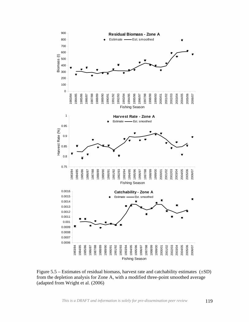
DDRRAAFFTTResidual Biomass - Zone A
0
100
200
300
400
500
600
700
800
900
1983
/84
1984
/85
1985
/86
1986
/87
1987
/88
1988
/89
1989
/90
1990
/91
1991
/92
1992
/93
1993
/94
1994
/95
1995
/96
1996
/97
1997
/98
1998
/99
1999
/00
2000
/01
2001
/02
2002
/03
2003
/04
2004
/05
2005
/06
2006
/07
Fishing Season
Bio
mas
s (t)
Estimate Est. smoothed
Harvest Rate - Zone A
0.75
0.8
0.85
0.9
0.95
1
1983
/84
1984
/85
1985
/86
1986
/87
1987
/88
1988
/89
1989
/90
1990
/91
1991
/92
1992
/93
1993
/94
1994
/95
1995
/96
1996
/97
1997
/98
1998
/99
1999
/00
2000
/01
2001
/02
2002
/03
2003
/04
2004
/05
2005
/06
2006
/07
Fishing Season
Har
vest
Rat
e (%
)
Estimate Est. smoothed
Catchability - Zone A
0.0006
0.0007
0.0008
0.0009
0.001
0.00110.0012
0.0013
0.0014
0.0015
0.0016
1983
/84
1984
/85
1985
/86
1986
/87
1987
/88
1988
/89
1989
/90
1990
/91
1991
/92
1992
/93
1993
/94
1994
/95
1995
/96
1996
/97
1997
/98
1998
/99
1999
/00
2000
/01
2001
/02
2002
/03
2003
/04
2004
/05
2005
/06
2006
/07
Fishing Season
Estimate Est. smoothed
Figure 5.5 – Estimates of residual biomass, harvest rate and catchability estimates (±SD) from the depletion analysis for Zone A, with a modified three-point smoothed average (adapted from Wright et al. (2006)
This is a DRAFT and information is solely for pre-dissemination peer review 119
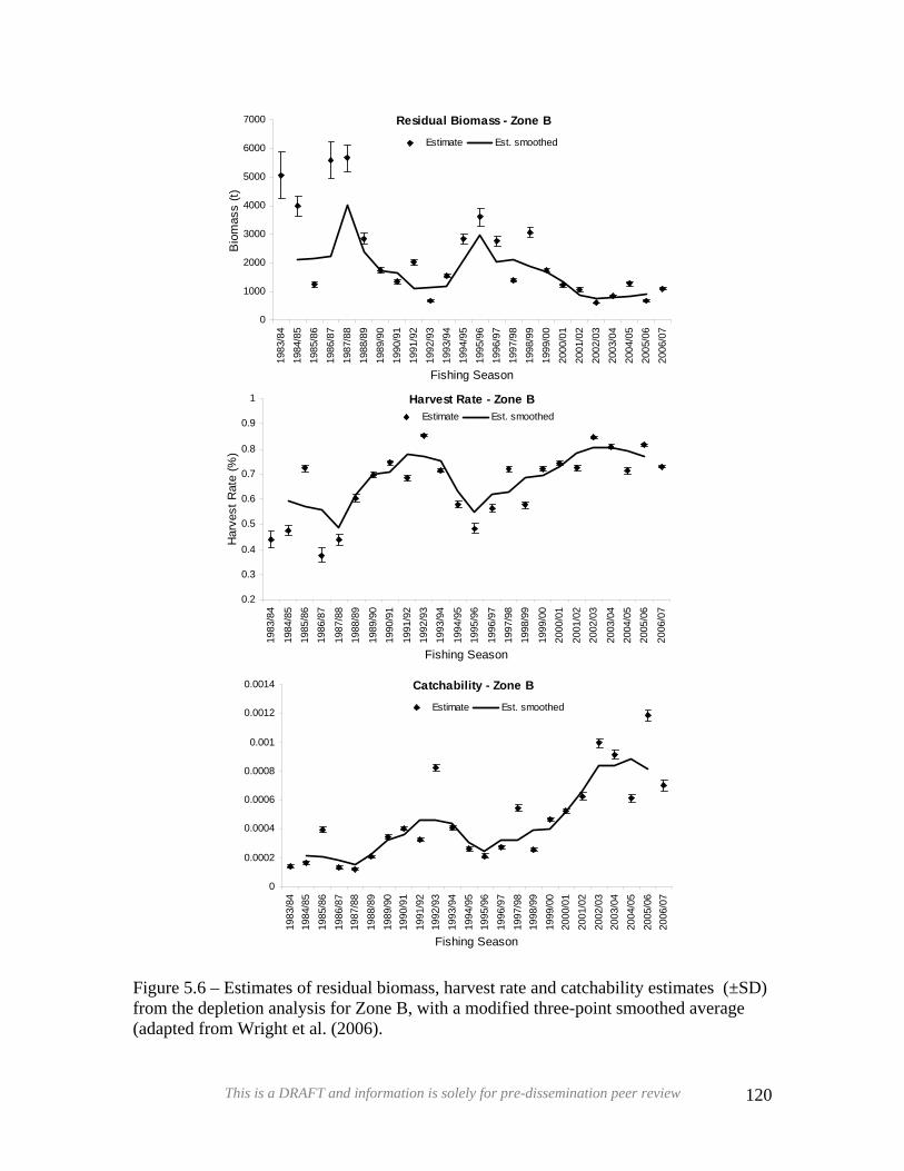
DDRRAAFFTTResidual Biomass - Zone B
0
1000
2000
3000
4000
5000
6000
7000
1983
/84
1984
/85
1985
/86
1986
/87
1987
/88
1988
/89
1989
/90
1990
/91
1991
/92
1992
/93
1993
/94
1994
/95
1995
/96
1996
/97
1997
/98
1998
/99
1999
/00
2000
/01
2001
/02
2002
/03
2003
/04
2004
/05
2005
/06
2006
/07
Fishing Season
Bio
mas
s (t)
Estimate Est. smoothed
Harvest Rate - Zone B
0.2
0.3
0.4
0.5
0.6
0.7
0.8
0.9
1
1983
/84
1984
/85
1985
/86
1986
/87
1987
/88
1988
/89
1989
/90
1990
/91
1991
/92
1992
/93
1993
/94
1994
/95
1995
/96
1996
/97
1997
/98
1998
/99
1999
/00
2000
/01
2001
/02
2002
/03
2003
/04
2004
/05
2005
/06
2006
/07
Fishing Season
Har
vest
Rat
e (%
)
Estimate Est. smoothed
Catchability - Zone B
0
0.0002
0.0004
0.0006
0.0008
0.001
0.0012
0.0014
1983
/84
1984
/85
1985
/86
1986
/87
1987
/88
1988
/89
1989
/90
1990
/91
1991
/92
1992
/93
1993
/94
1994
/95
1995
/96
1996
/97
1997
/98
1998
/99
1999
/00
2000
/01
2001
/02
2002
/03
2003
/04
2004
/05
2005
/06
2006
/07
Fishing Season
Estimate Est. smoothed
Figure 5.6 – Estimates of residual biomass, harvest rate and catchability estimates (±SD) from the depletion analysis for Zone B, with a modified three-point smoothed average (adapted from Wright et al. (2006).
This is a DRAFT and information is solely for pre-dissemination peer review 120
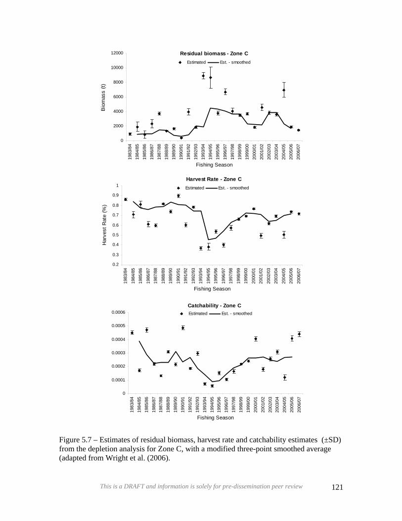
DDRRAAFFTTResidual biomass - Zone C
0
2000
4000
6000
8000
10000
12000
1983
/84
1984
/85
1985
/86
1986
/87
1987
/88
1988
/89
1989
/90
1990
/91
1991
/92
1992
/93
1993
/94
1994
/95
1995
/96
1996
/97
1997
/98
1998
/99
1999
/00
2000
/01
2001
/02
2002
/03
2003
/04
2004
/05
2005
/06
2006
/07
Fishing Season
Bio
mas
s (t)
Estimated Est. - smoothed
Harvest Rate - Zone C
0.2
0.3
0.4
0.5
0.6
0.7
0.8
0.9
1
1983
/84
1984
/85
1985
/86
1986
/87
1987
/88
1988
/89
1989
/90
1990
/91
1991
/92
1992
/93
1993
/94
1994
/95
1995
/96
1996
/97
1997
/98
1998
/99
1999
/00
2000
/01
2001
/02
2002
/03
2003
/04
2004
/05
2005
/06
2006
/07
Fishing Season
Har
vest
Rat
e (%
)
Estimated Est. - smoothed
Catchability - Zone C
0
0.0001
0.0002
0.0003
0.0004
0.0005
0.0006
1983
/84
1984
/85
1985
/86
1986
/87
1987
/88
1988
/89
1989
/90
1990
/91
1991
/92
1992
/93
1993
/94
1994
/95
1995
/96
1996
/97
1997
/98
1998
/99
1999
/00
2000
/01
2001
/02
2002
/03
2003
/04
2004
/05
2005
/06
2006
/07
Fishing Season
Estimated Est. - smoothed
Figure 5.7 – Estimates of residual biomass, harvest rate and catchability estimates (±SD) from the depletion analysis for Zone C, with a modified three-point smoothed average (adapted from Wright et al. (2006).
This is a DRAFT and information is solely for pre-dissemination peer review 121

DDRRAAFFTTIn modelling the recent trend is to use size-structured population models because of the
inability to age rock lobsters (Hobday and Punt 2007). In the western rock lobster fishery
the strong signal in the catch of lobsters with the puerulus settlement 3 and 4 years
previously, enables an age-structured model to be developed in which the growth
parameters in the model can be tuned so that the estimated catches are aligned with the
observed catches (see Stephenson and de Lestang in prep).
5.5 – Biological Modelling
In this assessment, a fine spatial scale of 8 inshore and 8 offshore areas was used to
mirror the different growth and maturity characteristics both onshore-offshore and along
the coast (Figure 5.8). A fine temporal scale of half monthly time steps was used to
capture the synchronous migration and the distinct temporal pattern of capture. In
addition, the fine temporal scale enables the evaluation of small temporal closures in the
management strategies on the stock and the economics of the fishery. This model is still
in the development stage and is planned for completion later this year and therefore full
diagnostics are not provided and information available at the time of release is presented.
The main characteristics of the new model are:
o Age/sex structured (with size composition outputs).
o Runs on a biological time scale (begins and ends with reproduction - 1st
November).
o Fine temporal scale - ½ month time step (day 1 – 14 and 15 +). Incorporates the
start of the season (coast and islands) and the start of the summer closure.
o Spatial scale - 16 separate transects/depth zones (<20 and 20+ fms).
o Contains a visual front end (graphics, maps and parameter estimates in Excel).
o Background programming in Ad Model Builder.
o Consists of six main sub-models and has the ability to turn these on/off.
o In the objective function contains commercial catch by year, area, and time-step
(Section 4.5), fishery independent and dependent breeding stock indices in each
region (Sections 4.2 and 4.3) and numbers of setose animals returned in each
management zone (Section 4.4 and 4.5).
This is a DRAFT and information is solely for pre-dissemination peer review 122
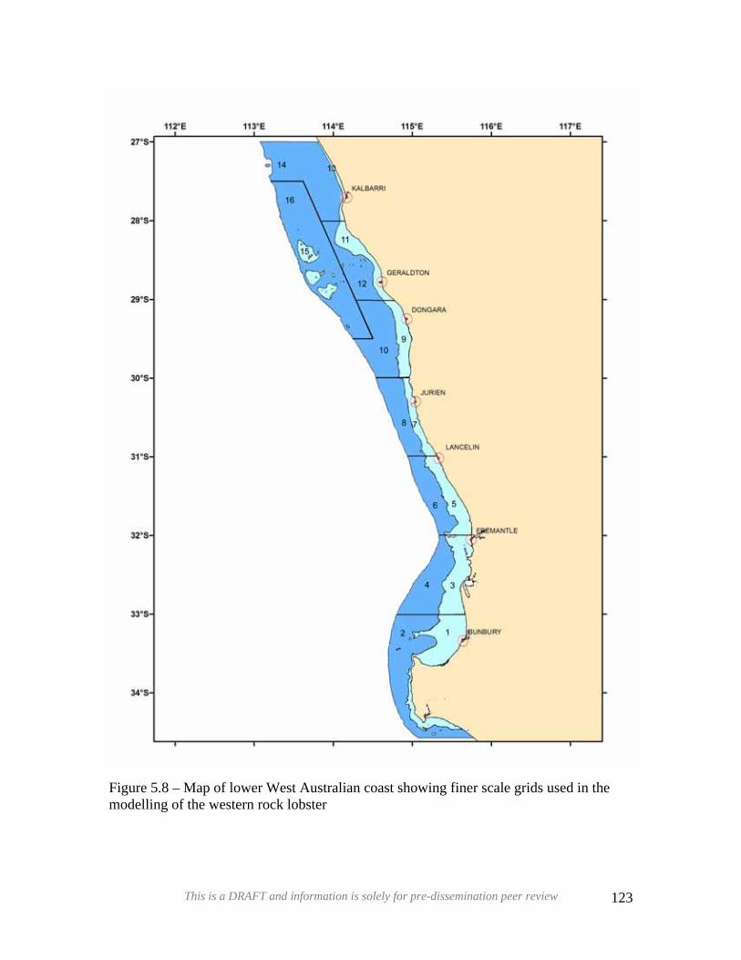
DDRRAAFFTT
Figure 5.8 – Map of lower West Australian coast showing finer scale grids used in the modelling of the western rock lobster
This is a DRAFT and information is solely for pre-dissemination peer review 123

5.5.1 – Methods
DDRRAAFFTTPopulation dynamics model
Recruitment
The lobsters are assumed to have a birth data of November 1 and this is taken as the
beginning of the first time step in the model. The number of lobsters (millions),
entering the fishery in each area of fishery,
syrN 1,2,,
γ , in each year, , at time-step t =1, and
length, L is given by
y
⎪⎩
⎪⎨⎧
=−
==
male)exp()1(
female)exp(
,
,,1,, sR
sRN
Ryrr
Ryrrs
Lyr ερ
ερ Eq. 5.4.11
where is the average recruitment in each area, rR γ , is a recruitment deviation term,
and
Ryr ,ε
ρ is the proportion of females.
The recruits have a normally distributed length (mm) of N(36, cv×36) where cv=0.1. This
length corresponds to approximately 2 years post settlement. The number of recruits are
distributed into length bins (Table 5.3) at the beginning of timestep t= 1
Table 5.3. The lower carapace length (mm) for each length bin used to store the number
of lobsters in each length class.
30 32 34 36 38 40 42 44 46 48 50
52 54 56 60 65 70 74 76 77 78 79
80 82 84 86 88 92 96 98 100 102 104
105 106 110 114 115 120 130
This is a DRAFT and information is solely for pre-dissemination peer review 124

DDRRAAFFTTThe annual variation in recruitment is tuned to puerulus deviation data derived from
puerulus counts from the collectors at Alkimos for 5,3,1=γ ; Lancelin for 7=γ , and
Seven Mile Beach for 15,13,11,9=γ . The puerulus deviations are given by
)119752006(
lnln
2006
1975,
,, +−−=
∑=y
yrr
yrrP
yr
PP
ωωε
The initial state in 1975 is
⎪⎩
⎪⎨
⎧
>−
≤=
−+−
+−+−
+−+−
++5for
1
5for
)1(
))(1(
,,1975,
))(1(,,1975,
1,1,1975,j
eeN
jeNN
Zij
KMijs
tjr
KMijstjr
stjr Eq. 5.4.2
where K is the initial equilibrium fishing mortality in 1975.
The exploitation rate on fully selected animals is fishing mortality, , is given by satyrF ,,,
yE
yrrtyrs
tjyr qEF ,,,,,,, )exp( γµε= Eq. 5.4.3
where is the effort (number of potlifts), is the average catchability, tyrE ,, rq yµ is the
efficiency increase, and is an effort deviation term. Eyr ,ε
This is a DRAFT and information is solely for pre-dissemination peer review 125
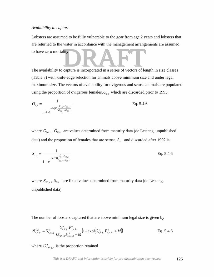
Availability to capture
DDRRAAFFTTLobsters are assumed to be fully vulnerable to the gear from age 2 years and lobsters that
are returned to the water in accordance with the management arrangements are assumed
to have zero mortality.
The availability to capture is incorporated in a series of vectors of length in size classes
(Table 3) with knife-edge selection for animals above minimum size and under legal
maximum size. The vectors of availability for ovigerous and setose animals are populated
using the proportion of ovigerous females, which are discarded prior to 1993 trO ,
( )rr
rf
tj
OOOLtrO
,50,95
,50,19ln,
e1
1
−
−−
+
= Eq. 5.4.6
where , are values determined from maturity data (de Lestang, unpublished
data) and the proportion of females that are setose, and discarded after 1992 is
rO ,50 rO ,95
trS ,
( )rr
rf
tj
SSSLtrS
,50,95
,50,19ln,
e1
1
−
−−
+
= Eq. 5.4.6
where , are fixed values determined from maturity data (de Lestang,
unpublished data)
rS ,50 rS ,95
The number of lobsters captured that are above minimum legal size is given by
(( MFGMFG
FGNN s
tjyrs
tjrstjyr
stjr
stjyr
stjrs
jtyrsG
tjyr +−+
= ,,,,,,,,,,,,
,,,,,,,,,
,,,, exp1 θ
θ
θ )) Eq. 5.4.6
where is the proportion retained stjrG ,,,θ
This is a DRAFT and information is solely for pre-dissemination peer review 126
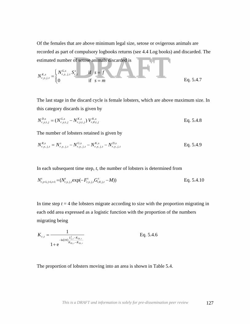
DRDRAAFFTT⎪⎩
⎪⎨⎧
=
==
ms
fsSNN
str
sGtjyrsK
tjyr if0
if,,
,,,,,,,
Of the females that are above minimum legal size, setose or ovigerous animals are
recorded as part of compulsory logbooks returns (see 4.4 Log books) and discarded. The
estimated number of setose animals discarded is
Eq. 5.4.7
The last stage in the discard cycle is female lobsters, which are above maximum size. In
this category discards is given by
sKjtr
sKjtyr
sGjtyr
sDjtyr VNNN ,
,,,,
,,,,
,,,,
,,, )( θ−= Eq. 5.4.8
The number of lobsters retained is given by
sDtjyr
sKtjyr
sGtjyr
stjyr
sRtjyr NNNNN ,
,,,,
,,,,
,,,,,,,
,,, −−−= Eq. 5.4.9
In each subsequent time step, t, the number of lobsters is determined from
))exp(( ,,,,,,,,,1,1,1, MGFNN stjr
stjyr
stjyr
stjyr −−=+++ θ Eq. 5.4.10
In time step t = 4 the lobsters migrate according to size with the proportion migrating in
each odd area expressed as a logistic function with the proportion of the numbers
migrating being
( )rr
rf
tj
KKKLtrK
,50,95
,50,19ln,
e1
1
−
−−
+
= Eq. 5.4.6
The proportion of lobsters moving into an area is shown in Table 5.4.
This is a DRAFT and information is solely for pre-dissemination peer review 127

Table 5.4. Matrix describing the source area and proportional distribution amongst
destination areas for migrating lobsters.
DDRAAFFTTR
To
Area 2 4 6 8 10 12 14 15
1 1 0 0 0 0 0 0 0
3 0 1 0 0 0 0 0 0
5 0 1 0 0 0 0 0 0
7 0 0 0 1 0 0 0 0
From 9 0 0 0 0 0.75 0 0 0.25
11 0 0 0 0 0 0.5 0 0.5
13 0 0 0 0 0 0 0.75 0.25
15 0 0 0 0 0 0 0 0
Egg Production
The major indicator of stock status is the egg production in regions 1=δ : southern
region (area 4, 6), 2=δ : northern region (areas 6, 8) and 3=δ : Abrolhos region (areas
15-16). For carapace length, , the egg production in time-step t =12 is given by fyL 12,
( ) ( )∑ ⋅⋅
⎟⎟⎟⎟
⎠
⎞
⎜⎜⎜⎜
⎝
⎛
+
+
+
=Θ−
−−
−
−−γ
δs
jyrdf
j
DD
DL
LL
LLy NLefj
fj
,12,,12,19ln19ln
,
5095
5012,
5095
5012,
e1
1
e1
1 Eq. 5.4.11
where the coefficient and power e = 1.92 and d = 2.69 (Chubb, 1991), and , , ,
are constants (Caputi 1995).
50L 95L 50D
95D
The management reference point is that the median value of the egg production index,
1980,
,,
δ
δδ Θ
Θ= y
yI should be > 1
This is a DRAFT and information is solely for pre-dissemination peer review 128
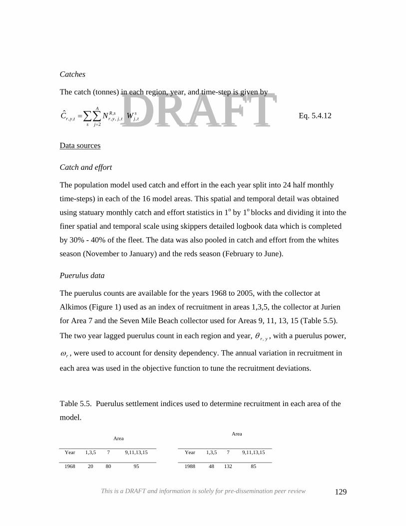
DDRAFT Eq. 5.4.12 RAFT∑∑=
=s
A
j
stj
sRtjyrtyr WNC
2,
,,,,,,
ˆ
Catches
The catch (tonnes) in each region, year, and time-step is given by
Data sources
Catch and effort
The population model used catch and effort in the each year split into 24 half monthly
time-steps) in each of the 16 model areas. This spatial and temporal detail was obtained
using statuary monthly catch and effort statistics in 1o by 1o blocks and dividing it into the
finer spatial and temporal scale using skippers detailed logbook data which is completed
by 30% - 40% of the fleet. The data was also pooled in catch and effort from the whites
season (November to January) and the reds season (February to June).
Puerulus data
The puerulus counts are available for the years 1968 to 2005, with the collector at
Alkimos (Figure 1) used as an index of recruitment in areas 1,3,5, the collector at Jurien
for Area 7 and the Seven Mile Beach collector used for Areas 9, 11, 13, 15 (Table 5.5).
The two year lagged puerulus count in each region and year, , with a puerulus power, yr ,θ
rω , were used to account for density dependency. The annual variation in recruitment in
each area was used in the objective function to tune the recruitment deviations.
Table 5.5. Puerulus settlement indices used to determine recruitment in each area of the
model.
Area Area
Year 1,3,5 7 9,11,13,15 Year 1,3,5 7 9,11,13,15
1968 20 80 95 1988 48 132 85
This is a DRAFT and information is solely for pre-dissemination peer review 129
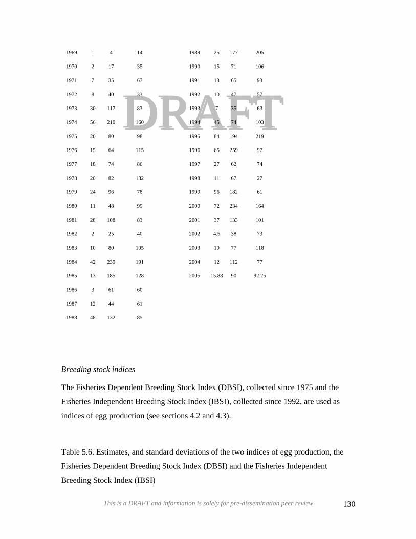
DDRRAFFTTA1993
1969 1 4 14 1989 25 177 205
1970 2 17 35 1990 15 71 106
1971 7 35 67 1991 13 65 93
1972 8 40 33 1992 10 47 57
1973 30 117 83 7 35 63
1974 56 210 160 1994 45 74 103
1975 20 80 98 1995 84 194 219
1976 15 64 115 1996 65 259 97
1977 18 74 86 1997 27 62 74
1978 20 82 182 1998 11 67 27
1979 24 96 78 1999 96 182 61
1980 11 48 99 2000 72 234 164
1981 28 108 83 2001 37 133 101
1982 2 25 40 2002 4.5 38 73
1983 10 80 105 2003 10 77 118
1984 42 239 191 2004 12 112 77
1985 13 185 128 2005 15.88 90 92.25
1986 3 61 60
1987 12 44 61
1988 48 132 85
Breeding stock indices
The Fisheries Dependent Breeding Stock Index (DBSI), collected since 1975 and the
Fisheries Independent Breeding Stock Index (IBSI), collected since 1992, are used as
indices of egg production (see sections 4.2 and 4.3).
Table 5.6. Estimates, and standard deviations of the two indices of egg production, the
Fisheries Dependent Breeding Stock Index (DBSI) and the Fisheries Independent
Breeding Stock Index (IBSI)
This is a DRAFT and information is solely for pre-dissemination peer review 130
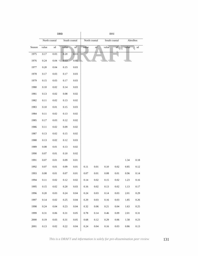
D AAFTTDRR F DBSI IBSI
North coastal South coastal North coastal South coastal Abrolhos
Season value sd value sd value sd value sd value sd
1975 0.17 0.03 0.20 0.03
1976 0.24 0.04 0.13 0.02
1977 0.20 0.04 0.15 0.03
1978 0.17 0.03 0.17 0.03
1979 0.15 0.03 0.17 0.03
1980 0.10 0.02 0.14 0.03
1981 0.13 0.02 0.08 0.02
1982 0.11 0.02 0.13 0.02
1983 0.10 0.01 0.15 0.03
1984 0.11 0.02 0.13 0.02
1985 0.17 0.03 0.12 0.02
1986 0.11 0.02 0.09 0.02
1987 0.13 0.02 0.15 0.02
1988 0.13 0.02 0.12 0.03
1989 0.08 0.01 0.13 0.02
1990 0.07 0.01 0.10 0.02
1991 0.07 0.01 0.09 0.01 1.34 0.18
1992 0.07 0.01 0.09 0.01 0.11 0.01 0.10 0.02 0.85 0.12
1993 0.08 0.01 0.07 0.01 0.07 0.01 0.08 0.01 0.96 0.14
1994 0.11 0.02 0.12 0.02 0.14 0.02 0.15 0.02 1.23 0.16
1995 0.15 0.02 0.20 0.03 0.16 0.02 0.13 0.02 1.13 0.17
1996 0.20 0.03 0.24 0.04 0.24 0.03 0.14 0.03 2.01 0.29
1997 0.14 0.02 0.25 0.04 0.29 0.03 0.16 0.03 1.85 0.26
1998 0.24 0.04 0.23 0.04 0.32 0.06 0.21 0.04 1.63 0.25
1999 0.31 0.06 0.31 0.05 0.78 0.14 0.46 0.09 2.01 0.31
2000 0.19 0.03 0.31 0.05 0.68 0.12 0.29 0.06 1.58 0.23
2001 0.13 0.02 0.22 0.04 0.24 0.04 0.16 0.03 0.86 0.13
This is a DRAFT and information is solely for pre-dissemination peer review 131
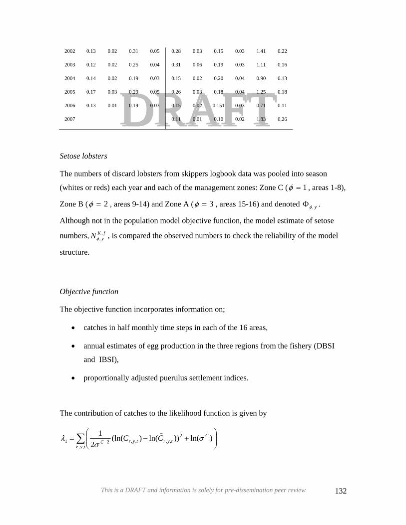
DRAAFTDR FT2002 0.13 0.02 0.31 0.05 0.28 0.03 0.15 0.03 1.41 0.22
2003 0.12 0.02 0.25 0.04 0.31 0.06 0.19 0.03 1.11 0.16
2004 0.14 0.02 0.19 0.03 0.15 0.02 0.20 0.04 0.90 0.13
2005 0.17 0.03 0.29 0.05 0.26 0.03 0.18 0.04 1.25 0.18
2006 0.13 0.01 0.19 0.03 0.15 0.02 0.151 0.03 0.71 0.11
2007 0.11 0.01 0.10 0.02 1.83 0.26
Setose lobsters
The numbers of discard lobsters from skippers logbook data was pooled into season
(whites or reds) each year and each of the management zones: Zone C ( 1=φ , areas 1-8),
Zone B ( 2=φ , areas 9-14) and Zone A ( 3=φ , areas 15-16) and denoted .
Although not in the population model objective function, the model estimate of setose
numbers, , is compared the observed numbers to check the reliability of the model
structure.
y,φΦ
fKyN ,
,φ
Objective function
The objective function incorporates information on;
• catches in half monthly time steps in each of the 16 areas,
• annual estimates of egg production in the three regions from the fishery (DBSI
and IBSI),
• proportionally adjusted puerulus settlement indices.
The contribution of catches to the likelihood function is given by
∑ ⎟⎟⎠
⎞⎜⎜⎝
⎛+−=
tyr
CtyrtyrC CC
,,
2,,,,21 )ln())ˆln()(ln(
21 σ
σλ
This is a DRAFT and information is solely for pre-dissemination peer review 132
The contribution of egg production from IBSI in each region to the likelihood function is
given by
DDRRAAFFTT∑ ⎟⎟
⎠
⎞
⎜⎜
⎝
⎛+Θ−Ω= Ω
Ωy
yyy
y,,
2,,2
,
2 )ln()))ln((ln(2
1δ
δδδ
δ
σσ
λ
The contribution of egg production from DBSI in each region to the likelihood function is
given by
∑ ⎟⎟
⎠
⎞
⎜⎜
⎝
⎛+Θ−Ψ−= Ψ
Ψy
yyy
y,,
2,,2
,
3 )ln())ln()ln((2
1δ
δδδ
δ
σσ
λ
The contribution of puerulus settlement deviations to the likelihood is
∑ ⎟⎟
⎠
⎞
⎜⎜
⎝
⎛+−=
yy
Ryr
Pyr
y,,
2,,2
,
3 )ln()(2
1δ
θδθ
δ
σεεσ
λ
The objective function, which is minimised in the model, consists of the negative of the
likelihood functions, together with the penalty functions as shown:
321 λλλλ ++= Eq. 5.4.13
Parameter values
Parameters assumed
The instantaneous rate of natural mortality, M, is 0.22 per year (Morgan 1995) which is
considerably higher than the value of 0.1 chosen by Punt and Kennedy (1997) for Jasus
edwardsii and that estimated by Starr et al. (1999) for Jasus edwardsii.
The value for the residual standard deviation of the catch data, Cσ , was assumed to be
0.5.
This is a DRAFT and information is solely for pre-dissemination peer review 133
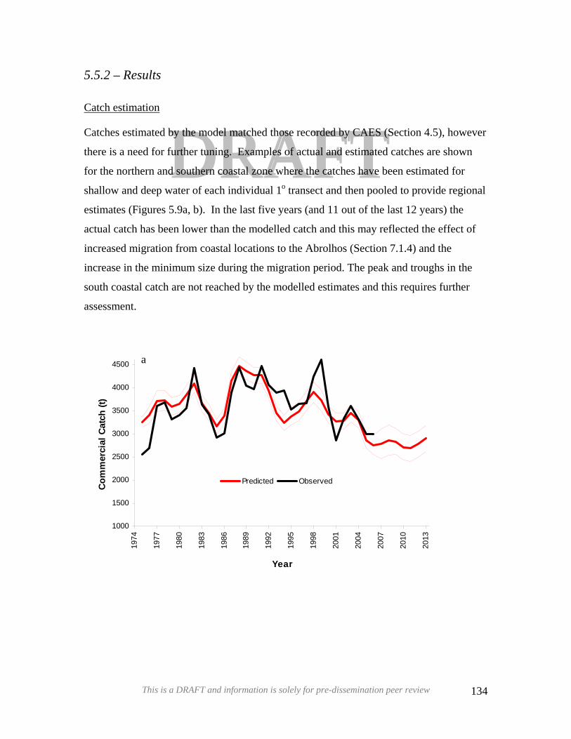
5.5.2 – Results
DDRRAAFFTTCatch estimation
Catches estimated by the model matched those recorded by CAES (Section 4.5), however
there is a need for further tuning. Examples of actual and estimated catches are shown
for the northern and southern coastal zone where the catches have been estimated for
shallow and deep water of each individual 1o transect and then pooled to provide regional
estimates (Figures 5.9a, b). In the last five years (and 11 out of the last 12 years) the
actual catch has been lower than the modelled catch and this may reflected the effect of
increased migration from coastal locations to the Abrolhos (Section 7.1.4) and the
increase in the minimum size during the migration period. The peak and troughs in the
south coastal catch are not reached by the modelled estimates and this requires further
assessment.
1000
1500
2000
2500
3000
3500
4000
4500
Com
mer
cial
Cat
ch (t
)
a1974
1977
1980
1983
1986
1989
1992
1995
1998
2001
2004
2007
2010
2013
Year
Predicted Observed
This is a DRAFT and information is solely for pre-dissemination peer review 134
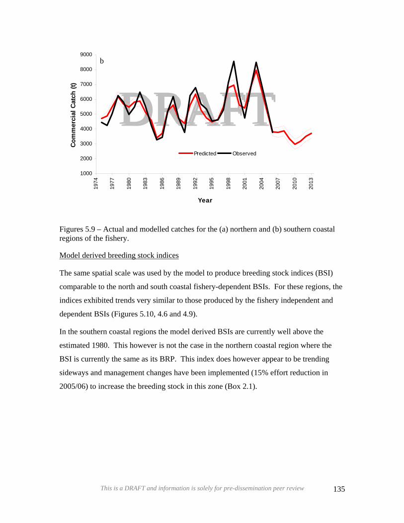
1000
2000
3000
4000
5000
6000
7000
8000
9000
Com
mer
cial
Cat
ch (t
)
Figures 5.9 regions of th
Model deriv
The same sp
comparable
indices exhi
dependent B
In the south
estimated 19
BSI is curre
sideways an
2005/06) to
b
DDRRAAFFTT19
74
1977
1980
1983
1986
1989
1992
1995
1998
2001
2004
2007
2010
2013
Year
Predicted Observed
– Actual and modelled catches for the (a) northern and (b) southern coastal e fishery.
ed breeding stock indices
atial scale was used by the model to produce breeding stock indices (BSI)
to the north and south coastal fishery-dependent BSIs. For these regions, the
bited trends very similar to those produced by the fishery independent and
SIs (Figures 5.10, 4.6 and 4.9).
ern coastal regions the model derived BSIs are currently well above the
80. This however is not the case in the northern coastal region where the
ntly the same as its BRP. This index does however appear to be trending
d management changes have been implemented (15% effort reduction in
increase the breeding stock in this zone (Box 2.1).
This is a DRAFT and information is solely for pre-dissemination peer review 135
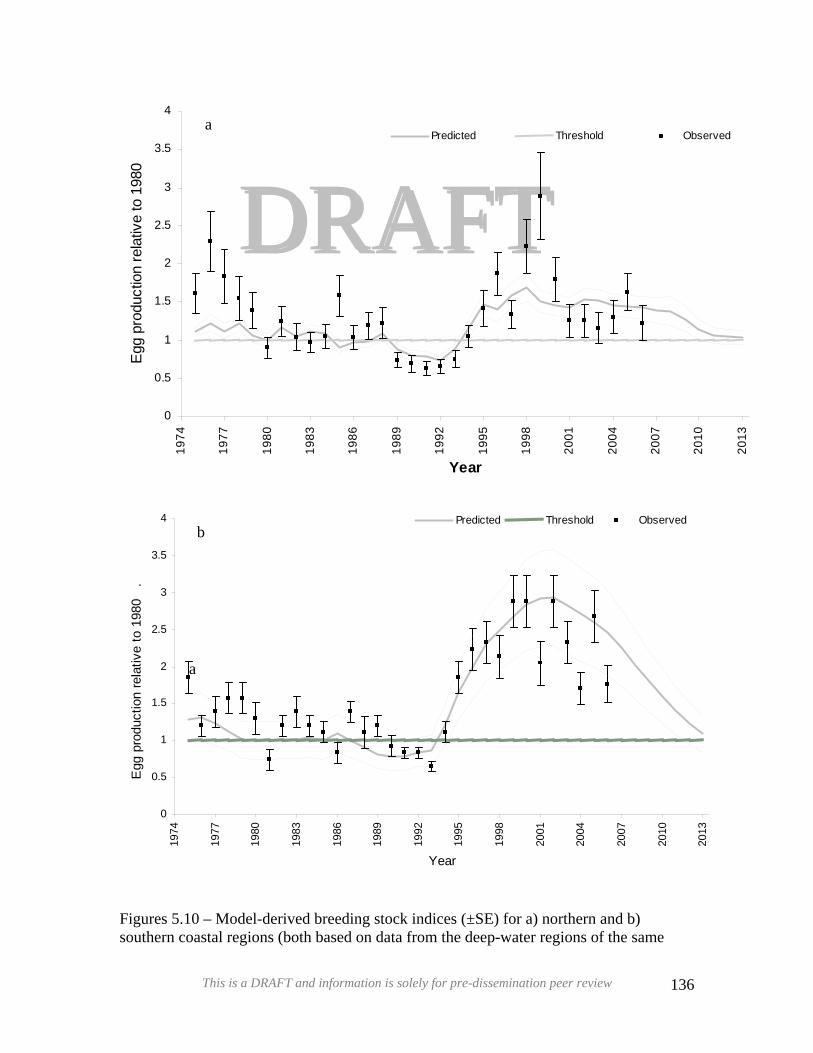
0
0.5
1
1.5
2
2.5
3
3.5
4
1974
Egg
pro
duct
ion
rela
tive
to 1
980
Predicted Threshold Observed
0
0.5
1
1.5
2
2.5
3
3.5
4
1974
Egg
pro
duct
ion
rela
tive
to 1
980
.
b
a
Figures 5.10southern coa
a
DDRRAAFFTT19
77
1980
1983
1986
1989
1992
1995
1998
2001
2004
2007
2010
2013
Year
1977
1980
1983
1986
1989
1992
1995
1998
2001
2004
2007
2010
2013
Year
Predicted Threshold Observed
– Model-derived breeding stock indices (±SE) for a) northern and b) stal regions (both based on data from the deep-water regions of the same
This is a DRAFT and information is solely for pre-dissemination peer review 136
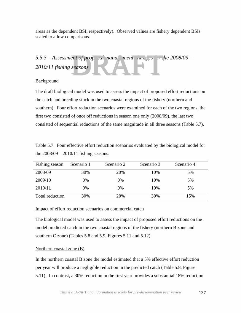
areas as the dependent BSI, respectively). Observed values are fishery dependent BSIs scaled to allow comparisons.
DD5.5.3 – Assessment of proposal management changes for the 2008/09 –
2010/11 fishing seasons
RRAAFFTTBackground
The draft biological model was used to assess the impact of proposed effort reductions on
the catch and breeding stock in the two coastal regions of the fishery (northern and
southern). Four effort reduction scenarios were examined for each of the two regions, the
first two consisted of once off reductions in season one only (2008/09), the last two
consisted of sequential reductions of the same magnitude in all three seasons (Table 5.7).
Table 5.7. Four effective effort reduction scenarios evaluated by the biological model for
the 2008/09 – 2010/11 fishing seasons.
Fishing season Scenario 1 Scenario 2 Scenario 3 Scenario 4
2008/09 30% 20% 10% 5%
2009/10 0% 0% 10% 5%
2010/11 0% 0% 10% 5%
Total reduction 30% 20% 30% 15%
Impact of effort reduction scenarios on commercial catch
The biological model was used to assess the impact of proposed effort reductions on the
model predicted catch in the two coastal regions of the fishery (northern B zone and
southern C zone) (Tables 5.8 and 5.9, Figures 5.11 and 5.12).
Northern coastal zone (B)
In the northern coastal B zone the model estimated that a 5% effective effort reduction
per year will produce a negligible reduction in the predicted catch (Table 5.8, Figure
5.11). In contrast, a 30% reduction in the first year provides a substantial 18% reduction
This is a DRAFT and information is solely for pre-dissemination peer review 137
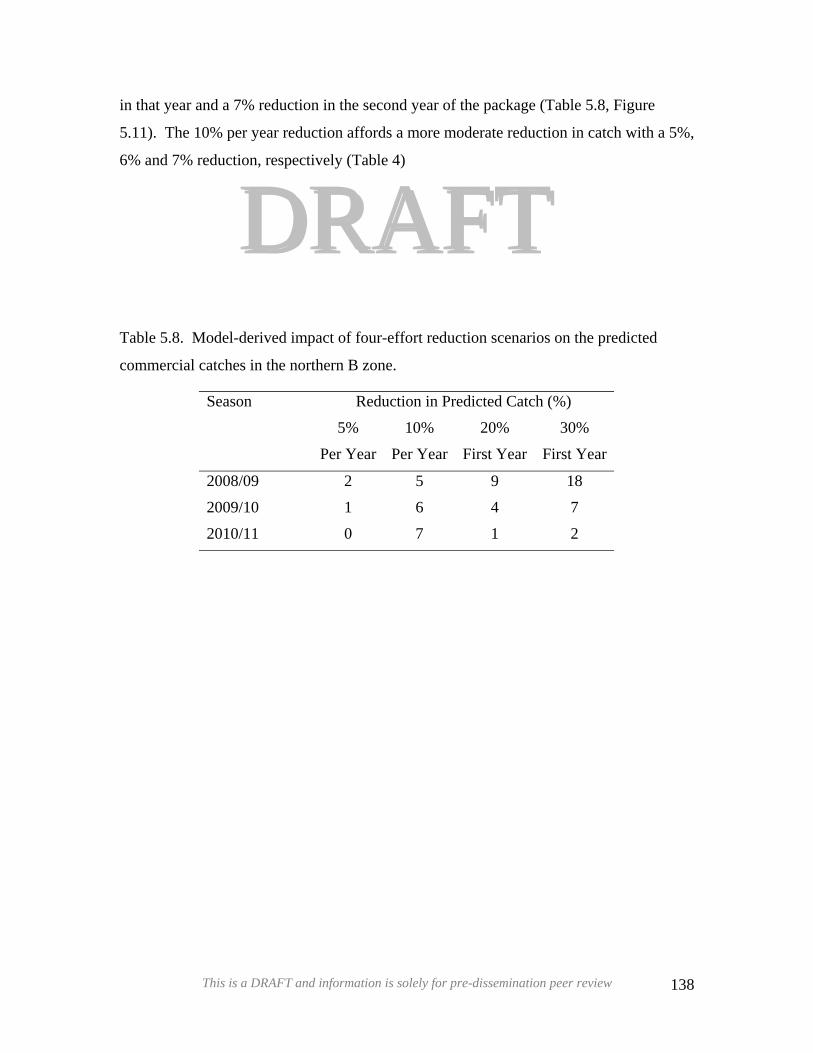
DDRRAAFFTTin that year and a 7% reduction in the second year of the package (Table 5.8, Figure
5.11). The 10% per year reduction affords a more moderate reduction in catch with a 5%,
6% and 7% reduction, respectively (Table 4)
Table 5.8. Model-derived impact of four-effort reduction scenarios on the predicted
commercial catches in the northern B zone.
Reduction in Predicted Catch (%) Season
5%
Per Year
10%
Per Year
20%
First Year
30%
First Year
2008/09 2 5 9 18
2009/10 1 6 4 7
2010/11 0 7 1 2
This is a DRAFT and information is solely for pre-dissemination peer review 138
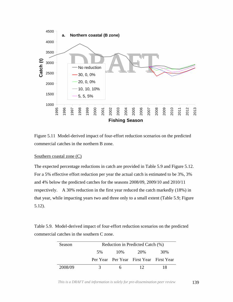
DDRRAAFFTTa. Northern coastal (B zone)
1000
1500
2000
2500
3000
3500
4000
4500
1995
1996
1997
1998
1999
2000
2001
2002
2003
2004
2005
2006
2007
2008
2009
2010
2011
2012
2013
Fishing Season
Cat
ch (t
)
No reduction
30, 0, 0%
20, 0, 0%
10, 10, 10%
5, 5, 5%
Figure 5.11 Model-derived impact of four-effort reduction scenarios on the predicted
commercial catches in the northern B zone.
Southern coastal zone (C)
The expected percentage reductions in catch are provided in Table 5.9 and Figure 5.12.
For a 5% effective effort reduction per year the actual catch is estimated to be 3%, 3%
and 4% below the predicted catches for the seasons 2008/09, 2009/10 and 2010/11
respectively. A 30% reduction in the first year reduced the catch markedly (18%) in
that year, while impacting years two and three only to a small extent (Table 5.9; Figure
5.12).
Table 5.9. Model-derived impact of four-effort reduction scenarios on the predicted
commercial catches in the southern C zone.
Reduction in Predicted Catch (%) Season
5%
Per Year
10%
Per Year
20%
First Year
30%
First Year
2008/09 3 6 12 18
This is a DRAFT and information is solely for pre-dissemination peer review 139
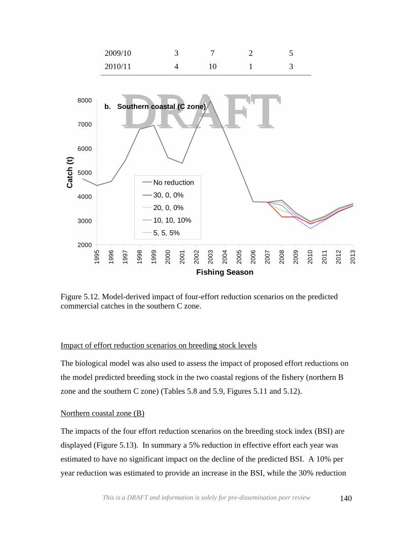
2009/10 3 7 2 5
2010/11 4 10 1 3
DDRRAAFFTTb. Southern coastal (C zone)
2000
3000
4000
5000
6000
7000
800019
95
1996
1997
1998
1999
2000
2001
2002
2003
2004
2005
2006
2007
2008
2009
2010
2011
2012
2013
Fishing Season
Cat
ch (t
)
No reduction
30, 0, 0%
20, 0, 0%
10, 10, 10%
5, 5, 5%
Figure 5.12. Model-derived impact of four-effort reduction scenarios on the predicted commercial catches in the southern C zone.
Impact of effort reduction scenarios on breeding stock levels
The biological model was also used to assess the impact of proposed effort reductions on
the model predicted breeding stock in the two coastal regions of the fishery (northern B
zone and the southern C zone) (Tables 5.8 and 5.9, Figures 5.11 and 5.12).
Northern coastal zone (B)
The impacts of the four effort reduction scenarios on the breeding stock index (BSI) are
displayed (Figure 5.13). In summary a 5% reduction in effective effort each year was
estimated to have no significant impact on the decline of the predicted BSI. A 10% per
year reduction was estimated to provide an increase in the BSI, while the 30% reduction
This is a DRAFT and information is solely for pre-dissemination peer review 140
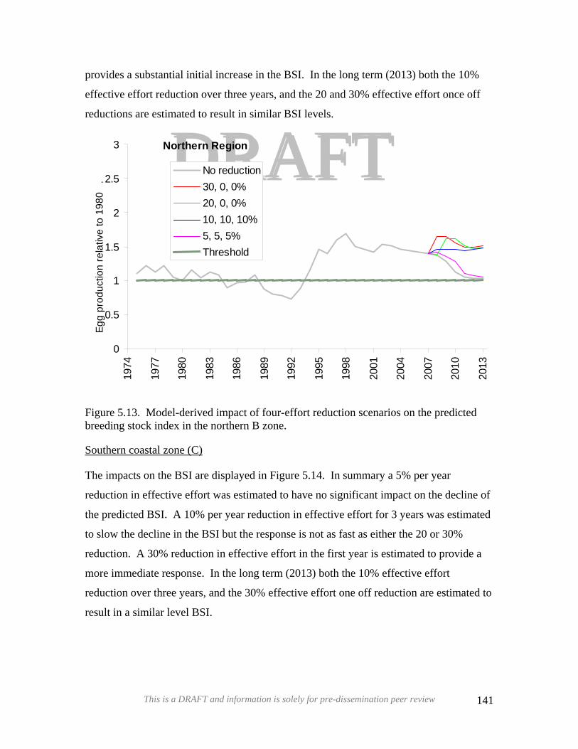
DDRRAAFFTTprovides a substantial initial increase in the BSI. In the long term (2013) both the 10%
effective effort reduction over three years, and the 20 and 30% effective effort once off
reductions are estimated to result in similar BSI levels.
Northern Region
0
0.5
1
1.5
2
2.5
319
74
1977
1980
1983
1986
1989
1992
1995
1998
2001
2004
2007
2010
2013
Egg
prod
uctio
n re
lativ
e to
198
0 .
No reduction30, 0, 0%20, 0, 0%10, 10, 10%5, 5, 5%Threshold
Figure 5.13. Model-derived impact of four-effort reduction scenarios on the predicted breeding stock index in the northern B zone.
Southern coastal zone (C)
The impacts on the BSI are displayed in Figure 5.14. In summary a 5% per year
reduction in effective effort was estimated to have no significant impact on the decline of
the predicted BSI. A 10% per year reduction in effective effort for 3 years was estimated
to slow the decline in the BSI but the response is not as fast as either the 20 or 30%
reduction. A 30% reduction in effective effort in the first year is estimated to provide a
more immediate response. In the long term (2013) both the 10% effective effort
reduction over three years, and the 30% effective effort one off reduction are estimated to
result in a similar level BSI.
This is a DRAFT and information is solely for pre-dissemination peer review 141
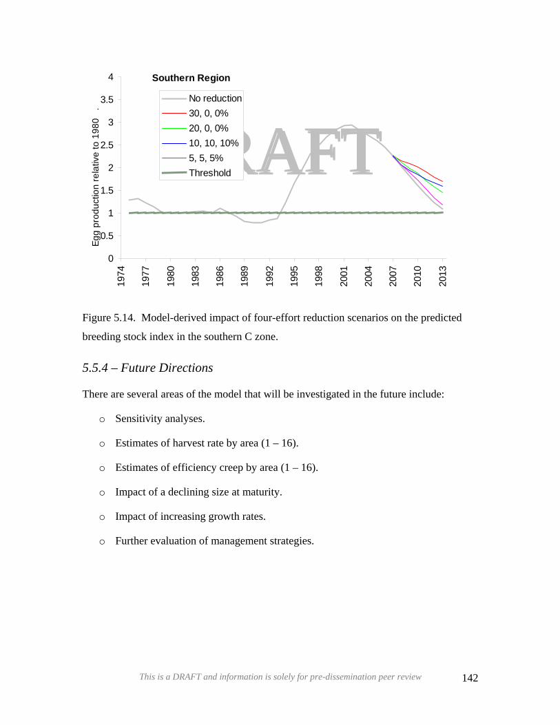
DDRRAAFFTTSouthern Region
0
0.5
1
1.5
2
2.5
3
3.5
4
1974
1977
1980
1983
1986
1989
1992
1995
1998
2001
2004
2007
2010
2013
Egg
prod
uctio
n re
lativ
e to
198
0 .
No reduction30, 0, 0%20, 0, 0%10, 10, 10%5, 5, 5%Threshold
Figure 5.14. Model-derived impact of four-effort reduction scenarios on the predicted
breeding stock index in the southern C zone.
5.5.4 – Future Directions
There are several areas of the model that will be investigated in the future include:
o Sensitivity analyses.
o Estimates of harvest rate by area (1 – 16).
o Estimates of efficiency creep by area (1 – 16).
o Impact of a declining size at maturity.
o Impact of increasing growth rates.
o Further evaluation of management strategies.
This is a DRAFT and information is solely for pre-dissemination peer review 142
DDRRAAFFTTEffective effort reductions (TAE) of 15 and 5% were recommended in Zones B and C,
respectively, for the 2005/06 to ensure breeding stock levels (Figure 4.6 and 4.8)
remained above their BRPs (Section 2.0). The management options for obtaining these
reductions included a number of temporal closures, legal-size changes and pot reductions,
with the combination of these employed were considered by industry (Box 2.1 –
2005/06). In order to assist in the decision process an economic model was developed by
the Department of Fisheries (Thomson & Caputi 2006) to assess the short-term (1-2
years) economic impacts of various effort reducing measures on the expected gross
margin of fishers in each zone.
5.6 – Economic Model
5.6.1 – Methods
Three management options were considered by the model; trap reductions, seasonal or
time closures and changes to the maximum size of females. These management options
have differing impacts on the biological, economic and social aspects of the fishery.
This project used average costs for fishers in each of the three zones and these were
obtained from the economic project evaluating input and output methods of management
for the rock lobster fishery undertaken by University of WA.
The impact on catch (and hence income) of the management options was undertaken
using an update of the Hall and Chubb (2001) model.
Pot Reductions
Pot reductions would achieve the required reduction in effort, with savings resulting in
terms of pot and bait usage. However, numbers of days fished would remain the same,
seeing little reduction, if any, in fuel costs. However, it may have longer-term effects
through rationalisation of the fleet, with licences being sold and fishers leaving the
industry. This may lead to improvement in the economic efficiency of the fleet, though
there are likely to be considerable transitional costs associated with redundant capital.
This is a DRAFT and information is solely for pre-dissemination peer review 143

Pot reductions for part of the season, during high catch periods, may also provide
improved prices for lobster and allow more orderly processing and marketing of lobster.
DDRRAAFFTTTime Closures
Focused around low catch periods, time closures have considerable savings in terms of
fuel and bait costs, while minimal impact on catches. Low catch periods identified were
in November, January, June and over full moon periods. They also provide social benefits
to the industry providing a rest period during the seven and a half month season.
Maximum Female Size Reduction
Lowering of the maximum size by 5 mm would provide direct protection for mature
females and improve breeding stock. However, this would have no economic advantages
in terms of operating costs.
5.6.2 – Results
The economic model assessment was to show which of the management options used
would provide the greatest effort reduction while minimising the short-term negative
economic impact on fishers.
The economic assessment was undertaken for the first two years of any proposed
management change, providing an initial impact of the management initiatives (year 1;
Figure 5.11) and also looking at the flow on effects in the following year (year 2; Figure
5.12).
This is a DRAFT and information is solely for pre-dissemination peer review 144
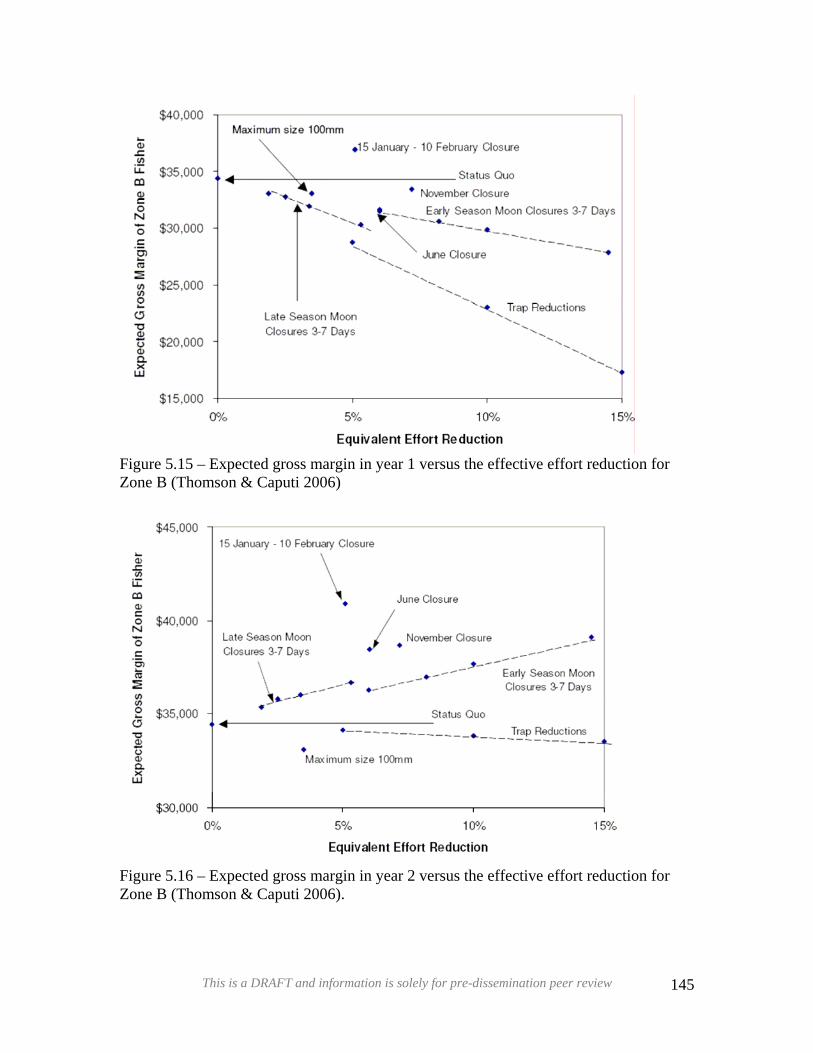
DDRRAAFFTT
Figure 5.15 – Expected gross margin in year 1 versus the effective effort reduction for Zone B (Thomson & Caputi 2006)
Figure 5.16 – Expected gross margin in year 2 versus the effective effort reduction for Zone B (Thomson & Caputi 2006).
This is a DRAFT and information is solely for pre-dissemination peer review 145
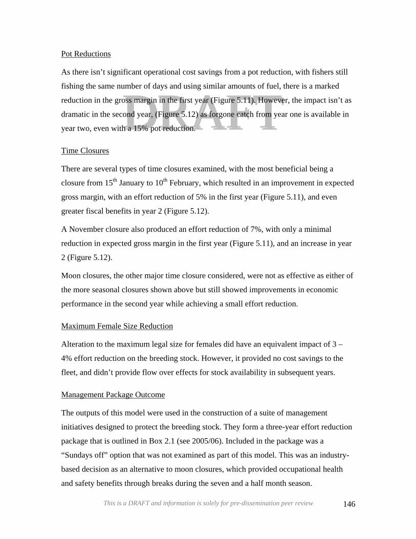
Pot Reductions
DDRRAAFFTTAs there isn’t significant operational cost savings from a pot reduction, with fishers still
fishing the same number of days and using similar amounts of fuel, there is a marked
reduction in the gross margin in the first year (Figure 5.11). However, the impact isn’t as
dramatic in the second year, (Figure 5.12) as forgone catch from year one is available in
year two, even with a 15% pot reduction.
Time Closures
There are several types of time closures examined, with the most beneficial being a
closure from 15th January to 10th February, which resulted in an improvement in expected
gross margin, with an effort reduction of 5% in the first year (Figure 5.11), and even
greater fiscal benefits in year 2 (Figure 5.12).
A November closure also produced an effort reduction of 7%, with only a minimal
reduction in expected gross margin in the first year (Figure 5.11), and an increase in year
2 (Figure 5.12).
Moon closures, the other major time closure considered, were not as effective as either of
the more seasonal closures shown above but still showed improvements in economic
performance in the second year while achieving a small effort reduction.
Maximum Female Size Reduction
Alteration to the maximum legal size for females did have an equivalent impact of 3 –
4% effort reduction on the breeding stock. However, it provided no cost savings to the
fleet, and didn’t provide flow over effects for stock availability in subsequent years.
Management Package Outcome
The outputs of this model were used in the construction of a suite of management
initiatives designed to protect the breeding stock. They form a three-year effort reduction
package that is outlined in Box 2.1 (see 2005/06). Included in the package was a
“Sundays off” option that was not examined as part of this model. This was an industry-
based decision as an alternative to moon closures, which provided occupational health
and safety benefits through breaks during the seven and a half month season.
This is a DRAFT and information is solely for pre-dissemination peer review 146

5.6.3 – Future Direction
DRAFTCurrently a more-detailed economic model is being developed to assist in future
management decisions. This model should evaluate long-term (5 years) as well as the
short-term economic impacts. Eventually, outputs from this model will be used, in
consultation with stakeholders, to decide on the most economically and socially
beneficial management package to address the biological changes in the breeding stock.
It is planned that this economic model will be linked to the biological model so that there
is a biological and economic assessment of any proposed management change.
DRAFT
This is a DRAFT and information is solely for pre-dissemination peer review 147

6 – Biological Reference Points and Stock Status
DRAFTDRAFTIn a discussion paper released in 2004, a decision framework was proposed for the
WCRLMF (Bray 2004). This framework was designed to provide flexibility,
transparency and accountability, and advances the concept of co-management in the
management system.
6.1 – Management Decision Framework
6.1.1 – Background
The basis of the decision framework is to address a number of objectives in bringing
about changes to the management regime. The specific objectives (after Bray (2004)) are:
o Biological objective: That management arrangements maintain or return to, as
the case may be, the abundance of breeding lobsters at or above the levels in 1980
(Biological Reference Point (BRP)).
o Ecological objective: That management arrangements are consistent with the
principles of ecosystem-based fisheries management and in particular:
o Ensure that by-catch of marine mega-fauna is minimised
o That the effects of fishing do not result in irreversible changes to the
ecological processes.
o Commercial objectives: (i) That management arrangements maximise the
opportunity for optimum economic returns to the Western Australian community
from the use of the western rock lobster resource. (ii) That management
arrangements foster the maintenance and development of regional communities
while not unnecessarily restricting normal business practices.
o Recreational objective : That management arrangements which impact upon the
recreational fishery promote the fundamental ethos of recreational fishing, i.e. it is
an enjoyment motivated activity.
This is a DRAFT and information is solely for pre-dissemination peer review 148
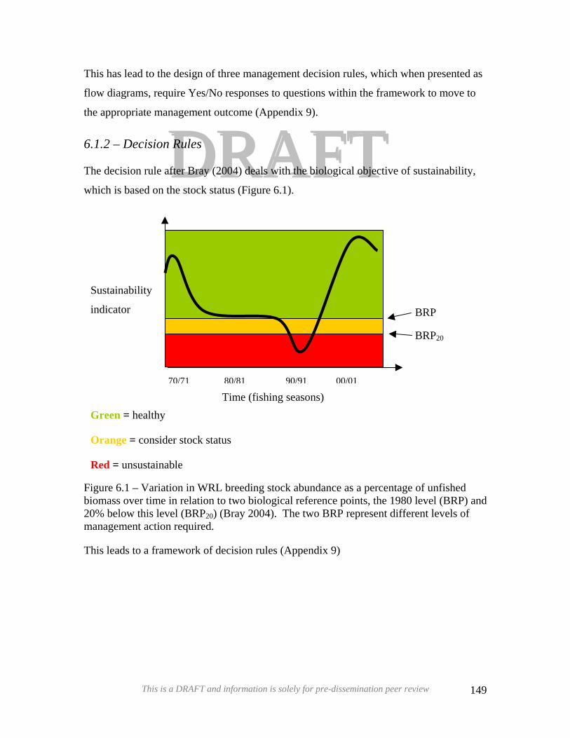
DDRRAAFFTTThis has lead to the design of three management decision rules, which when presented as
flow diagrams, require Yes/No responses to questions within the framework to move to
the appropriate management outcome (Appendix 9).
6.1.2 – Decision Rules
The decision rule after Bray (2004) deals with the biological objective of sustainability,
which is based on the stock status (Figure 6.1).
BRP
BRP20
Green = healthy
Orange = consider stock status
Red = unsustainable
Sustainability
indicator
00/0190/9180/8170/71
Time (fishing seasons)
Figure 6.1 – Variation in WRL breeding stock abundance as a percentage of unfished biomass over time in relation to two biological reference points, the 1980 level (BRP) and 20% below this level (BRP20) (Bray 2004). The two BRP represent different levels of management action required.
This leads to a framework of decision rules (Appendix 9)
This is a DRAFT and information is solely for pre-dissemination peer review 149
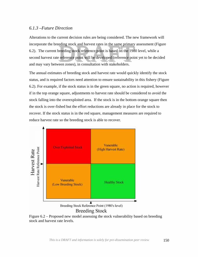
6.1.3 –Future Direction
DDRRAAFFTTAlterations to the current decision rules are being considered. The new framework will
incorporate the breeding stock and harvest rates in the same primary assessment (Figure
6.2). The current breeding stock reference point is based on the 1980 level, while a
second harvest rate reference point will be developed (reference point yet to be decided
and may vary between zones), in consultation with stakeholders.
The annual estimates of breeding stock and harvest rate would quickly identify the stock
status, and is required factors need attention to ensure sustainability in this fishery (Figure
6.2). For example, if the stock status is in the green square, no action is required, however
if in the top orange square, adjustments to harvest rate should be considered to avoid the
stock falling into the overexploited area. If the stock is in the bottom orange square then
the stock is over-fished but the effort reductions are already in place for the stock to
recover. If the stock status is in the red square, management measures are required to
reduce harvest rate so the breeding stock is able to recover.
Figure 6.2 – Proposed new model assessing the stock vulnerability based on breeding stock and harvest rate levels.
This is a DRAFT and information is solely for pre-dissemination peer review 150

6.2 – Stock Status
DRAFTThe status of the lobster stocks in each of the three management zones (A – C) is assessed
annually based on trends exhibited by a number of empirical and model-derived indices.
These include fishery-dependent (Section 4.2), fishery-independent (Section 4.3) and
modelled (Section 5.5) indices of breeding stock (BSI), log-book estimates of the setose
female biomass (Section 4.4), depletion-based estimates of residual biomass, harvest rate
and efficiency increases (Section 5.4) and model-derived estimates of annual efficiency
increases (Section 5.5). The primary performance indicator of stock status is currently
the BSI relative to its estimate during the 1980/81 fishing season for the north and south
coastal zones (Biological Reference Point - BRP). The use of multiple indices allows for
the cross checking of general trends, with agreement increasing assessment confidence or
disagreement highlighting areas that need further assessment.
DRAFT
This is a DRAFT and information is solely for pre-dissemination peer review 151
6.2.1 – Stock Status by Zone (2005/06 fishing season)
Zone A
DDRRAAFFTTo The catch in this fishery in the 2004/05 and 2005/06 season have been the two
highest on record for this region. As the size at maturity is below the legal size
and the fishery opens (15 March) after spawning has completed in the late
spring/summer and followed by a moult in about February, catch has been used
historically as an indication of the spawning stock
o The full season harvest rate is currently estimated at 85% based on the depletion
analysis, which is down on the maximum of 92% recorded in the 1999/00 fishing
season (Section 5.4). Although the harvest rate is high, being significantly below
its maximum, suggests this level is sustainable. A BRP does not currently exist
for this parameter.
o Residual legal biomass remaining at the end of the fishing season was estimated at
614 t, which in the highest level recorded (Section 5.4).
o A efficiency increase occurred after the 18% pot reduction in 1993/94 that may be
due to pot saturation effect (Section 5.4).
o The numbers of setose females returned to the water has been increasing since the
1993/94, with the 2004/05 season recording the highest estimate before a slight
downturn in the last season to 1.82 million (2005/06) (Section 4.4).
o The fishery-independent BSI has declined in recent years and needs to be
monitored (Section 4.3).
o The model-derived BSI is currently well above the its estimated 1980 level and
trending sideways (Section 5.5).
The above indices indicate that in Zone A the stock is heavily exploited, however
given the trend in the catch and that spawning occurs below the size at maturity, its
breeding component is considered to be at a healthy level. A BRP needs to be set for
the Zone A BSI and harvest rate.
This is a DRAFT and information is solely for pre-dissemination peer review 152
Zone B
DRRAAFFTTDo The full season harvest rate, adjusted for the 1993/94 package, has increased
progressively since 1995/96 before levelling off at ~80% over the past the seasons
(Section 5.4). This level is considered high. A BRP does not exist for this
parameter.
o The residual legal biomass estimated to remain at the end of the fishing season
has declined rapidly from high levels in 1995/96 (~2800t) to level off at below
800t in the last three seasons (Section 5.4). A BRP does not exist for this
parameter.
o Efficiency has been increasing rapidly over the past ten years (Section 5.4).
o Approximately 0.96 million setose females were returned to the water in 2005/06.
After peaking in 1999/00, numbers declined to a low in 2002/03, before
recovering slightly and then declining again (Section 4.4).
o The fishery-dependent BSI is currently above its threshold BRP (1980 level),
although its closeness to this level and recent downward trend warrant concern
(Section 4.2).
o The fishery-independent BSI reinforces the status indicated by the fishery
dependent BSI, i.e. the condition of the breeding stock is of concern (Section 4.3).
o The model-derived BSI is currently just below its estimated 1980 level, agreeing
with both fishery-dependent and independent BSIs (Section 5.5).
The above indices indicate that the stock in Zone B is heavily exploited and its
breeding component is close to the BRP threshold level. This stock is considered
vulnerable, and management changes (15% effort reduction in 2005/06) have
occurred to improve its status, however it will take 2-3 years for the effect of this to
be seen in the spawning stock (Box 2.1). A BRP needs to be set for the Zone B
harvest rate.
This is a DRAFT and information is solely for pre-dissemination peer review 153
Zone C
DRAFTDRAFTo The full season harvest rate, adjusted for the 1993/94 package, has increased only
slightly over recent seasons and currently resides at ~ 70% (Section 5.4). This
level is considered sustainable. A BRP does not exist for this parameter.
o The residual legal biomass estimated to remain at the end of the fishing season
declined slightly this season to 2800t but still remains above the early 1990’s level
(Section 5.4). A decline from this level would be of concern.
o Depletion analysis indicates that there has been an increase in fishing efficiency in
this region over the past ten years but lower that zone B (Section 5.4).
o The number of setose females returned to the water in 2005/06, has increased
from the previous season, and is still at almost record high levels (Section 4.4).
o The fishery-dependent BSI is currently far above its threshold BRP (1980 level)
and appears relatively stable (Section 4.2).
o The fishery-independent BSI reinforces the status indicated by the fishery
dependent BSI, however, it is above the BRP by a lesser amount than the
dependent BSI (Section 4.3).
o The model-derived BSI is currently well above its estimated 1980 level, which
supports the trends exhibited by the fishery dependent and independent BSIs
(Section 5.5).
Catch in 2005/06 was below average and below-average catches are predicted until
2009/10 as a result of a series of low puerulus settlement due to weak or average Leeuwin
Currents since 2000. This may result in a decline in spawning stock in the future.
The above indices suggest the Zone C stock is moderately exploited while its
breeding component remains above the BRP threshold level. This stock is considered
healthy, although with four years of predicted low recruitment, steps have been taken
to keep this stock above threshold levels (Section 2). A BRP needs to be set for the
Zone C harvest rate.
This is a DRAFT and information is solely for pre-dissemination peer review 154
7 – Current Research
DDRRAAFFTTThere are several projects that are currently at various stages of completion. These
address a variety of research issues dealing with the effective management of the
WCRLF. Project objectives are outlined below. All pertinent results will be reported on
in future editions of this document.
7.1.1 – Reproductive Biology Pertinent to Brood Stock Management
The protection of setose females and large females through a maximum size limit (Box
2.2) may have distorted the sex ratios of breeding lobster. With a scarcity of males of
similar size, maximum size females are presumably having to mate with smaller males,
which has, in laboratory studies, been shown to lead to brood size reductions in other
lobster species (MacDiarmid and Butler 1999). The WRL FRDC project (with Melville-
Smith at Principal Investigator) aims to investigate the implications of the protection of
maximum size females to provide preliminary information on possible reduced egg size
at the Abrolhos Islands compared to coastal sites, and to quantify the extent of the
breeding grounds to weight egg production for the stock by the three management zones
based on these interactions.
7.1.2 – Lobster Movement Through Acoustic Tracking
Acoustic tracking is a relatively new technique that allows detailed information on
movement patterns, habitat usage and home ranges for aquatic species. This technology is
currently being applied to the western rock lobster, to examine their movement behaviour
in deep-water environments. Two tracking experiments have been undertaken in waters
>50 m off Dongara and Jurien Bay, where 8 and 12 lobsters have been tracked for 90 and
70 days, respectively. Analysis is currently underway on both tracking sessions
examining the foraging behaviour, in terms of timing and habitats utilised, as well as
home range areas.
This is a DRAFT and information is solely for pre-dissemination peer review 155

7.1.3 – Effects of Closed Areas
DRAFTDRAFTA monitoring program has just been initiated to examine the impacts of fishing activities
on WRL and their associated benthic habitats. This project will examine abundance, size
and sex state compositions of lobsters inside and outside of sanctuary zones in shallow
water sites in Jurien and off the Perth metropolitan coast. Monitoring consists of
capturing lobsters in commercial batten lobster traps with enclosed escape gaps (Section
4.3), with lobsters sexed, measured, maturity condition recorded (i.e. external eggs) and
tagged with a spaghetti tag before being returned to location of capture. Divers will
conduct underwater visual surveys in the same locations to provide an alternative
measure of lobster abundance and size composition. These surveys will run concurrently
with benthic habitat and invertebrate/fish surveys.
Possible outcomes of this work will include;
i. An improved understanding on what virgin shallow-water lobster stocks may
have been like in abundance and size structure;
ii. Information on whether no-take zones may be any use in the sustainable
management of this species;
iii. Information about whether all lobsters move into deep water; and
iv. Growth rate data, unbiased by size-related catchability/reporting issues.
This is a DRAFT and information is solely for pre-dissemination peer review 156
7.1.4 – Climate Change
DRAFTDRAFTEnvironmental factors (Section 4.7) have been shown to have a significant effect on this
lobster fishery. The south-flowing Leeuwin Current and the strength of westerly winds in
late winter/spring have been shown to significantly affect the level of puerulus settlement
(Section 4.1). The strength of the Leeuwin Current is influenced by the frequency of
ENSO events. A strong Leeuwin Current is associated with warmer temperature and a
strong eddy structure (which may affect primary production as measured by the
chlorophyll levels) off the coast of Western Australia. Climate change may be causing an
increasing trend in water temperature, a weakening of the westerly winds in
winter/spring, an increase in the frequency of ENSO events, and an increase in the sea
level. These factors can affect the level and spatial distribution in puerulus settlement,
size at maturity, size of migrating lobsters, growth rates, catchability of the western rock
lobster, numbers of mature females moulting from setose to non-setose condition, timing
of moults and hence the timing of the peak catch rates. Some of these changes may have
negative implications on the western rock lobster fishery but some such as increasing
water temperature may have some positive influence. This project will asses the impact
that climate change may be having on the environmental factors that affect the rock
lobster fishery such as water temperature, frequency of ENSO events, Leeuwin Current
strength, westerly winds and their implications for the western rock lobster fishery.
This is a DRAFT and information is solely for pre-dissemination peer review 157
8 – Recommendations for Future Research
DDRRAAFFTTo There are indications that some effects of climate change (e.g. water temperature
increases) may be affecting some aspects of the biology of the WRL such as size
at maturity, whites migration, setose moult, catchability, and puerulus settlement.
These need to be assessed and appropriate trends built into the assessment models
to assess the effect on the stock status. There is also a need to understand future
trends in climate change provided by climate models and assess the implication
for the lobster fishery.
There are several areas that are being considered for future research. These include
o Understanding of aspects of the Leeuwin Current variability (water temperature,
productivity, eddy structure) that is contributing to the variation in puerulus
settlement.
o Assessment of ways to improve pot efficiency that can be used to improvement of
the economic performance of the fishery and minimise the ecological impact of
pot fishing
o Economic modelling to assess management measures to improve the economic
performance of the fishery
o Further assessment of the biological model e.g. sensitivity analysis, assessment of
management options, future projections, suitability for developing of BRP
o Testing improved escape gaps to minimise fishery-induced mortality of undersize
lobsters
o Natural mortality, migration and carrying capacity (abundance and size structure)
assessments in closed areas including proposed closed areas in deep water
o Review of estimates of fishing efficiency from different models
o Review and development of BRP for harvest rate and spawning stock for each
region
This is a DRAFT and information is solely for pre-dissemination peer review 158

9 – References
DDRRAAFFTTBray, T. 2004. Development of a fisheries management decision rules framework for the
west coast rock lobster fishery. DRAFT Report on behalf of the Rock Lobster Industry
Advisory Committee
Braaten, D.O. 1969 Robustness of DeLury population estimation. Journal of Fisheries
Research, Board of Canada 26: 339-355
Brown, R. S. and Caputi, N. 1986. Conservation of recruitment of the western rock
lobster (Panulirus cygnus) by improving survival and growth of undersize rock lobsters
captured and returned by fishermen to the sea. Canadian Journal of Fisheries and
Aquatic Sciences 43: 2236-2242.
Brown, R. S., Caputi, N., and Barker, E. 1995. A preliminary assessment of increases
in fishing power on stock assessment and fishing effort expended in the western rock
lobster (Panulirus cygnus) fishery. Crustaceana 68: 227-237.
Bureau of Meteorology 2007. Monthly rainfall review Australia– April 2007, Bureau of
Meteorology, Australian Government
Caputi, N. in press. Impact of the Leeuwin Current on the spatial distribution of the
puerulus settlement of the western rock lobster (Panulirus cygnus) fishery of Western
Australia. Fisheries Oceanography.
Caputi, N. and Brown, R. 1986. Relationship between indices of juvenile abundance
and recruitment in the western rock lobster (Panulirus cygnus) fishery Canadian Journal
of Fisheries and Aquatic Science 43(11) 2131-2139
Caputi, N., Brown, R. S., and Phillips, B. F. 1995a. Predicting catches of the western
rock lobster (Panulirus cygnus) based on indices of puerulus and juvenile abundance.
ICES Marine Science Symposium. 199: 287-293.
This is a DRAFT and information is solely for pre-dissemination peer review 159

DRAFTCaputi, N., Chubb, C., Hall, N. and Brown, R. 2000. Measurement of catch and fishing
effort in the Western Rock Lobster fishery. In Spiny Lobsters: Fisheries and Culture
(Eds. B. Phillips and J. Kittaka) pp 334-356, Blackwell Science, Oxford, U.K. DRAFT
Caputi, N., Chubb, C., and Brown, R. 1995b. Relationships between spawning stock,
environment and fishing effort for the Western Rock Lobster Panulirus cygnus, fishery in
Western Australia Crustaceana 68(2): 213-226
Caputi, N., Chubb, C., and Pearce, A. 2001. Environmental effects on recruitment of
the western rock lobster, Panulirus cygnus. Marine and Freshwater Research 52: 1167-
1174.
Chittleborough, R. G. 1974a. Home Range, Homing, and Dominance in Juvenile
Western Rock Lobsters. Australian Journal of Marine and Freshwater Research. 25:
227-234.
Chittleborough, R. G. 1974b. Western rock lobster reared to maturity. Australian
Journal of Marine and Freshwater Research. 25: 211-215.
Chittleborough, R. G. 1975. Environmental factors affecting growth and survival of
juvenile western rock lobsters Panulirus longipes (Milne-Edwards) Journal of Marine
and Freshwater Research. 26: 177-196.
Chittleborough, R. G. 1976a. Breeding of Panulirus longipes cygnus under natural and
controlled conditions. Journal of Marine and Freshwater Research. 27: 499-516.
Chittleborough, R. G. 1976b. Growth of juvenile Panulirus longipes cygnus (George)
on coastal Reefs compared with those reared under optimal environmental conditions.
Journal of Marine and Freshwater Research. 27, 279-295.
Chittleborough, R. and Phillips, B. 1975. Fluctuations of year-class strength and
recruitment in the Western Rock Lobster Panulirus longipes (Milne-Edwards) along the
Western Australian coast. Australian Journal of Marine and Freshwater Research
26(3):317-328
This is a DRAFT and information is solely for pre-dissemination peer review 160

Chubb, C. F. 1991. Measurement of spawning stock levels for the western rock lobster,
Panulirus cygnus. Revista de Investigaciones Marinas 12: 223-233.
DChubb, C. F., Rossbach, M., Melville-Smith, R., and Cheng, Y. W. 1999. Mortality,
growth and movement of the western rock lobster (Panulirus cygnus). Final Report
FRDC Project No. 95/020. DRRAAFFTTCox, D.R. and Miller, H.D. 1965. The theory of stochastic processes Chapman and Hall,
London. Pp 146-156
de Lestang, S. Caputi, N. and Melville-Smith, R. in prep. Using fine scale catch
predictions to examine spatial variation in growth and catchability of Panulirus cygnus
along the west coast of Australia
de Lestang, S. and Melville-Smith, R. 2006. Interannual variation in the moult cycle
and size at double breeding of mature female western rock lobster (Panulirus cygnus).
ICES Journal of Marine Science 63: 1631-1639.
Delury, D.B. 1947. On the estimation of biological populations. Biometrics 3: 145-167
Department of Fisheries 2005. Integrated Fisheries Management Report Western Rock
Lobster. Fisheries Management Report No. 192, Department of Fisheries Western
Australia
Edgar, G. J. 1990. Predator prey interactions in seagrass beds .1. The influence of
macrofaunal abundance and size structure on the diet and growth of the western rock
lobster Panulirus cygnus George. Journal of Experimental Marine Biology and Ecology
139: 1-22.
Fogarty, M.J. and Idoine, J.S. 1988. Application of a yield and egg production model
based upon size to an offshore American lobster population. Transactions of the
American Fisheries Society 117: 350-62
This is a DRAFT and information is solely for pre-dissemination peer review 161

DGray, H. 1999. The Western Rock Lobster Panulirus cygnus Book 2: A History of the
Fishery, Westralian Books DRRAAFFTTFernandez, J. A., Cross, J. M., and Caputi, N. 1997. The impact of Technology on
fishing power in Western Rock Lobster (Panulirus cygnus) Fishery. International
Congress on Modeling and Simulation Proceedings (MODSIM 97) 4:
Grey, K. A. 1979. Estimates of the size of first maturity of the Western rock lobster,
Panulirus cygnus, using secondary sexual characteristics [Western Australia]. Australian
.Journal of .Marine and .Freshwater Research 30: 785-791.
Hall, N. and Chubb, C. 2001. The status of the western rock lobster, Panulirus cygnus,
fishery and the effectiveness of management controls in increasing the egg production of
the stock, Marine and Freshwater Research 52(8): 1657-1667
Hobday, D. and Punt, A.E. 2007. Spatial modelling and assessment of the Victorian
Southern Rock Lobster (Jasus edwardsii) fishery. Final Report FRDC Project No.
2004/037
IFAAC 2007. Integrated Fisheries Management Allocation Report – Western Rock
Lobster Resource Fisheries Management Report No. 218, Integrated Fisheries Allocation
Advisory Committee, Department of Fisheries, Western Australia
Jernakoff, P. 1987. Foraging patterns of juvenile western rock lobsters Panulirus cygnus
George. Journal of Experimental Marine Biology and Ecology 113: 125-144.
Jernakoff, P. and Phillips, B. F. 1988. Effect of a baited trap on the foraging
movements of juvenile western rock lobsters Panulirus cygnus George.
Aust.J.Mar.Freshwater Res. 39: 185-192.
Jernakoff, P., Phillips, B. F., and Maller, R. A. 1987. A quantitative study of nocturnal
foraging distances of the West Australian rock lobster, Panulirus cygnus George. Journal
of Experimental Marine Biology and Ecology 113: 9-21.
This is a DRAFT and information is solely for pre-dissemination peer review 162

DRJohnson, R.A. and Wichern, D.W. 1982. Applied multivariate statistical analysis
Prentice Hall, New York. Pp 291-357 DRAAFFTTJohnson, M. S. 1999. Temporal variation of recruits as a basis of ephemeral genetic
heterogeneity in the western rock lobster Panulirus cygnus. Marine Biology (Berlin) 135:
133-139.
Joll, L. M. and Phillips, B. F. 1984. Natural diet and growth of juvenile Western rock
lobsters Panulirus cygnus George. Journal of Experimental Marine Biology and Ecology
75: 145-169.
Kendall, M. and Stuart, A. 1973. The advanced theory of statistics Volume 2. Charles
Griffin, London. Pp 330-360
Leslie, P.H. and Davis, D.H.S 1939. An attempt to estimate the absolute number of rats
on a given area. Journal of Animal Ecology 8: 94-113
Lipcius, R. N. and Cobb, J. S. 1994 Ecology and fishery biology of spiny lobsters. In
Spiny Lobsters: Fisheries and Culture (Eds. B. Phillips and J. Kittaka) pp 1-30,
Blackwell Science, Oxford, U.K.
MacDiarmid, A.B. and Butler, M.J. IV 1999. Sperm economy and limitation in spiny
lobsters, Behavioural Ecology and Sociobiology, 46: 14-24.
Melville-Smith, R. and Anderton, S. M. 2000. Western rock lobster mail surveys of
licensed recreational fishers 1986/87 to 1998/ 99. Fisheries Research Report No. 122, pp
1-39. Perth, Australia, Department of Fisheries Western Australia
Melville-Smith, R., Anderton, S. M., and Caputi, N. 2001. Predicting the recreational
western rock lobster (Panulirus cygnus) catch in Western Australia. Marine and
Freshwater Research 52: 1527-1534.
Melville-Smith, R. and Chubb, C. F. 1997. Comparison of dorsal and ventral tag
retention in western rock lobster, Panulirus cygnus (George). Marine and Freshwater
Research 48: 577-580.
This is a DRAFT and information is solely for pre-dissemination peer review 163

DRAFTMelville-Smith, R. and de Lestang, S. 2006. Spatial and temporal variation in the size at
maturity of the western rock lobster Panulirus cygnus George. Marine Biology (Berlin)
150: 183-195.
DRAFTMelville-Smith, R., Chubb, C., Caputi, N., Cheng, Y. W., Christianopoulos, D., and
Rossbach, M. 1998. Fishery independent survey of the breeding stock and migration of
the western rock lobster (Panulirus cygnus . FRDC Project 96/108 Final Report, pp 1-47.
Perth, Australia, Fisheries Western Australia.
Melville-Smith, R., and de Lestang, S. 2007. Changes in egg production of the western
rock lobster (Panulirus cygnus) associated with appendage damage. Fisheries Bulletin
105: 418–425.
Melville-Smith, R., Thomson, A. W., and Caputi, N. 2004. Improved forecasts of
recreational western rock lobster (Panulirus cygnus) catches in Western Australia, by
predicting license usage. Fisheries Research 68: 203-208.
Morgan, G. R. 1972. Fecundity in the western rock lobster Panulirus longipes cygnus
(George)(Crustacea: Decapoda: Palinuridae. Australian Journal of Marine and
Freshwater Research. 23: 133-141.
Morgan, G. R. 1974. Aspects of the population dynamics of the western rock lobster,
Panulirus cygnus George. II. Seasonal changes in the catchability coefficient. Australian
Journal of Marine and Freshwater Research 25: 249-259.
Morgan, G. R. 1977. Aspects of the Population Dynamics of the Western Rock Lobster
and their Role in Management. PhD Thesis. University of Western Australia.
Muller, R.G., Hunt, J. H., Matthews, T.R. and Sharp, W.C. 1997 Evaluation of effort
reductions in the Florida Keys spiny lobster, Panulirus argus, fishery using an age-
structured population analysis. Marine and Freshwater Research 48:1045-1058
Phillips, B. F., Palmer, M. J., Cruz, R., and Trendall, J. T. 1992. Estimating growth of
the Spiny Lobsters Panulirus cygnus, P.argus and P.ornatus. Aust.J.Mar.Freshwater Res.
43: 1177-1188.
This is a DRAFT and information is solely for pre-dissemination peer review 164

DRAFTPearce, A. F. and Phillips, B. F. 1988. ENSO events, the Leeuwin Current, and larval
recruitment of the western rock lobster. Journal du Conseil 45: 13-21 DRAFTMorgan, G. R, Phillips, B. and Joll, L. 1982. Stock and recruitment relationships in
Panulirus cygnus, the commercial rock (Spiny) lobster of Western Australia Fishery
Bulletin 80(3): 475-486
Phillips, B. F. 1972. A semi-quantitative collector of the puerulus larvae of the western
rock lobster Panulirus longipes cygnus (George) (Decapoda, Palinuridae. Crustaceana
22: 147-154.
Phillips, B. F. 1981. The circulation of the southeastern Indian Ocean and the planktonic
life of the western rock lobster. Oceanography and Marine Biology. An Annual Review
19: 11-39
Phillips, B. F. 1986. Prediction of commercial catches of the western rock lobster
Panulirus cygnus Canadian Journal of Fisheries and Aquatic Science 43(11) 2126-2130
Phillips, B. F. and MacMillan, D. L. 1987. Antennal receptors in puerulus and
postpuerulus stages of the rock lobster Panulirus cygnus (Decapoda: Palinuridae) and
their potential role in puerulus navigation. Journal of Crustacean Biology 7: 122-135.
Phillips, B. and Melville-Smith, R. 2006. Panulirus Species. In Lobsters: Biology,
Management, Aquaculture and Fisheries (Ed B. Phillips) pp 359-384, Blackwell Science,
Oxford, U.K.
Phillips, B. and Olson, L. 1975. The swimming behaviour of the puerulus stage of
WRL. Australian Journal of Marine and Freshwater Research 26:415-417
Phillips, B., Pearce, A. and Litchfield, R. 1991 The Leeuwin Current and larval
recruitment to the rock (spiny) lobster fishery off Western Australia. Journal of the Royal
Society of Western Australia 74: 93-100
This is a DRAFT and information is solely for pre-dissemination peer review 165

DDRRAAFFTTPunt, A.E., Kennedy, R.B. and Frusher, S. 1997. Estimating the size-transition matrix
for Tasmanian rock lobster, Jasus edwardsii. Marine and Freshwater Research 48: 981-
992
Ross, S.M. 1985 Introduction to probability models. Academic Press, Orlando, Florida,
USA. Pp 196-204
Ricker, W.E. 1975. Computation and interpretation of biological statistics of fish
populations. Bulletin of Fisheries Research, Board of Canada 191:149-161
SAS Institute Inc. 1987. SAS/STAT Guide for Personal Computers, Version 6 Edition.
Cary, NC: SAS Institute Inc. 1028 pp.
Spiegelhalter, D.J., Thomas, A., Best, N. and Gilks, W.R. 1996 BUGS0.5, Bayesian
inference using Gibbs sampling Manual. Medical Research Council Biostatistics Unit,
Institute of Public Health. Cambridge, UK.
Srisurichan, S. 2001. Time series modeling of the environmental factors affecting the
daily catch rate of western rock lobster. Unpublished MSc Thesis Edith Cowan
University, Perth, Western Australia
Srisurichan, S., Caputi, N., and Cross, J. 2005. Impact of lunar cycle and swell on the
daily catch rate of western rock lobster (Panulirus cygnus) using time series modeling.
New Zealand Journal of Marine and Freshwater Research 39: 749-764.
Starr, P.J., Breeen, P.A., Hilborn, R. and Kendrick, T.H. 1997 Evaluation of a
management decision rule for a New Zealand rock lobster substock. Marine and
Freshwater Research 48: 1093-1101
Thomson, A. W. and Melville-Smith, R. 2005. Have different inducements used with
the western rock lobster mail survey of recreational licensees had an effect on total catch
estimates? North American Journal of Fisheries Management 25: 1203-1207.
This is a DRAFT and information is solely for pre-dissemination peer review 166

DRAFTThompson, A. P., Hanley, J. R., and Johnson, M. S. 1996. Genetic structure of the
western rock lobster, Panulirus cygnus, with the benefit of hindsight. Marine and
Freshwater Research 47: 889-896. DRAFT
Thomson, N. and Caputi, N. 2006. An economic analysis of management options in the
western rock lobster fishery of Western Australia. Fisheries Centre Research Reports 14:
157-164.
Waddington, K., Bellchambers, L., Vanderklift, M. and Walker, D. in prep. Diet of
adult western rock lobster (Panulirus cygnus) populations in Western Australian deep
coastal ecosystems (35-60m).
Wright, I., Caputi, N., and Penn, J. 2006. Depletion-based population estimates for
western rock lobster (Panulirus cygnus) fishery in Western Australia. New Zealand
Journal of Marine and Freshwater Research 40: 107-122.
This is a DRAFT and information is solely for pre-dissemination peer review 167
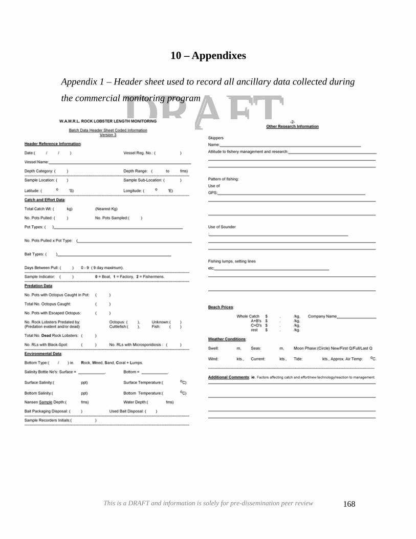
10 – Appendixes
DDRRAAFFTTAppendix 1 – Header sheet used to record all ancillary data collected during
the commercial monitoring program
This is a DRAFT and information is solely for pre-dissemination peer review 168
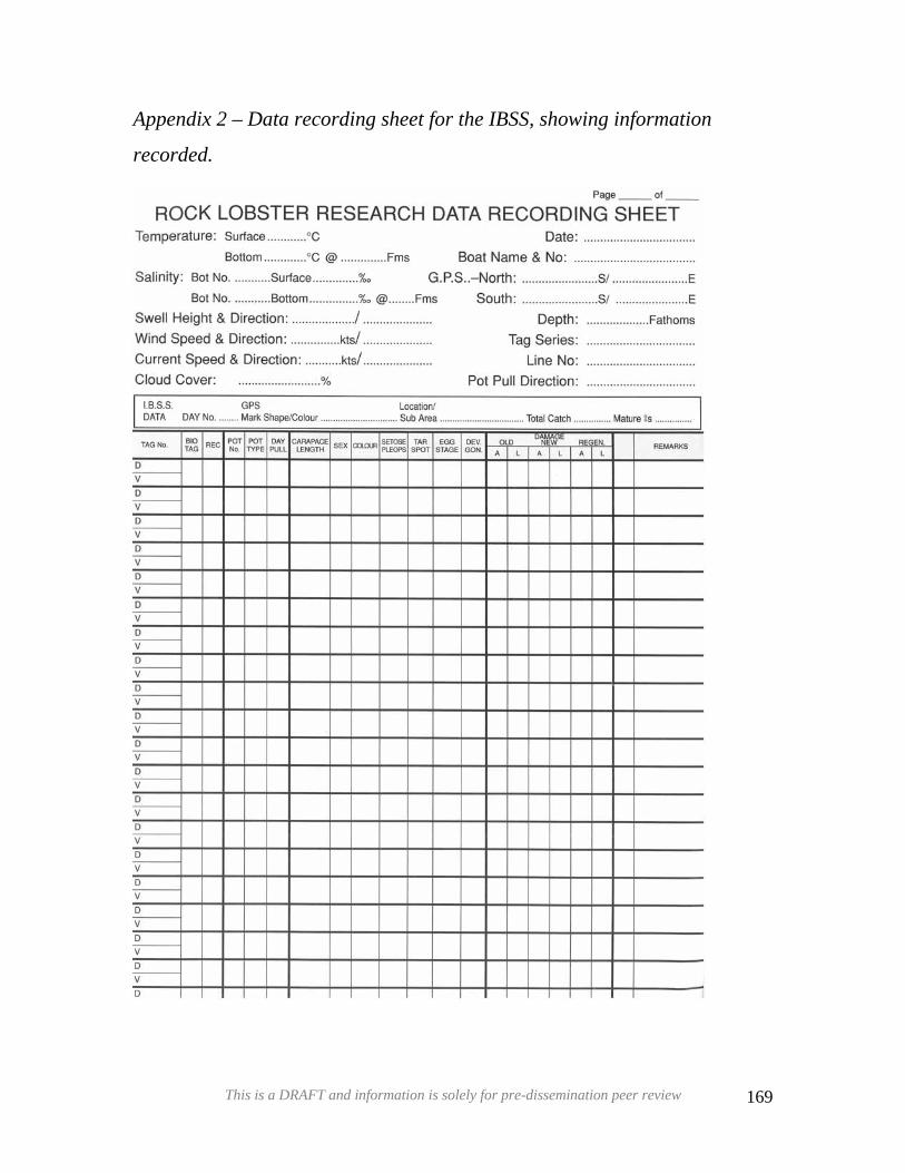
Appendix 2 – Data recording sheet for the IBSS, showing information
recorded.
DDRRAAFFTT
This is a DRAFT and information is solely for pre-dissemination peer review 169
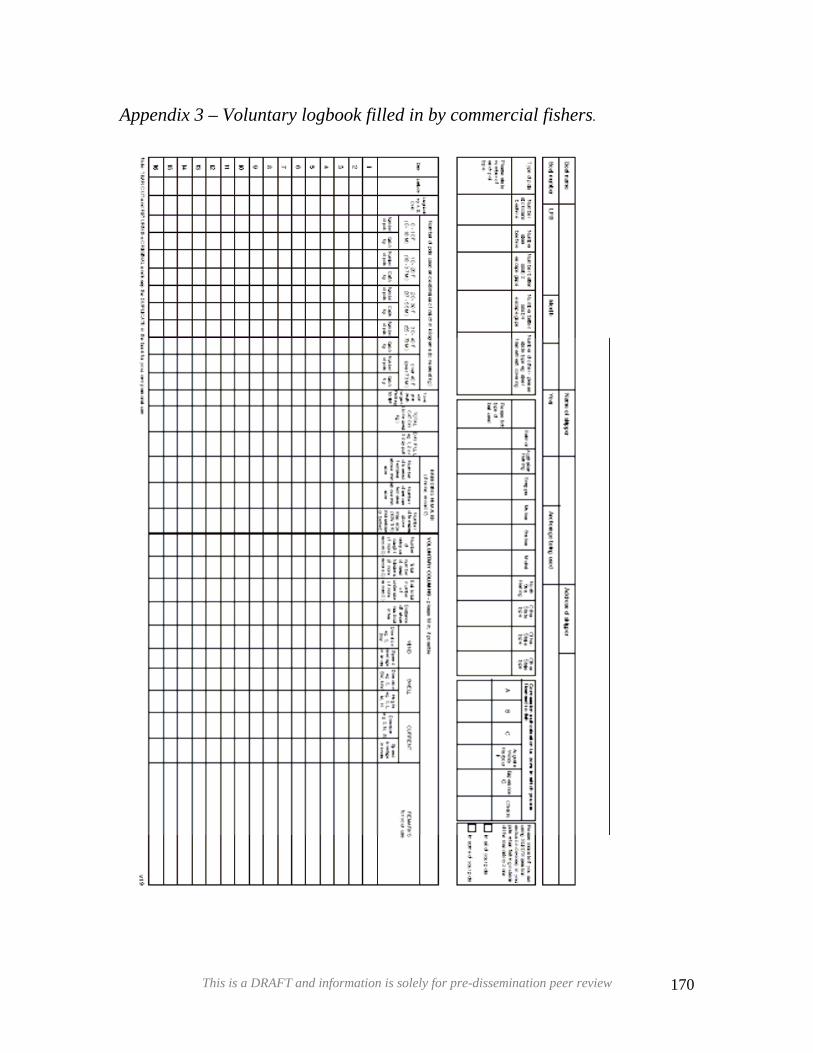
Appendix 3 – Voluntary logbook filled in by commercial fishers.
DDRRAAFFTT
This is a DRAFT and information is solely for pre-dissemination peer review 170
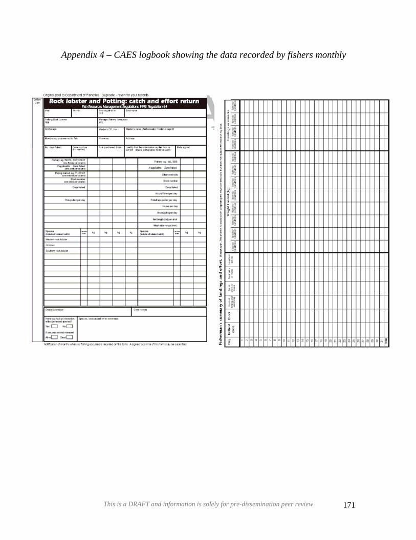
Appendix 4 – CAES logbook showing the data recorded by fishers monthly
DDRRAAFFTT
This is a DRAFT and information is solely for pre-dissemination peer review 171
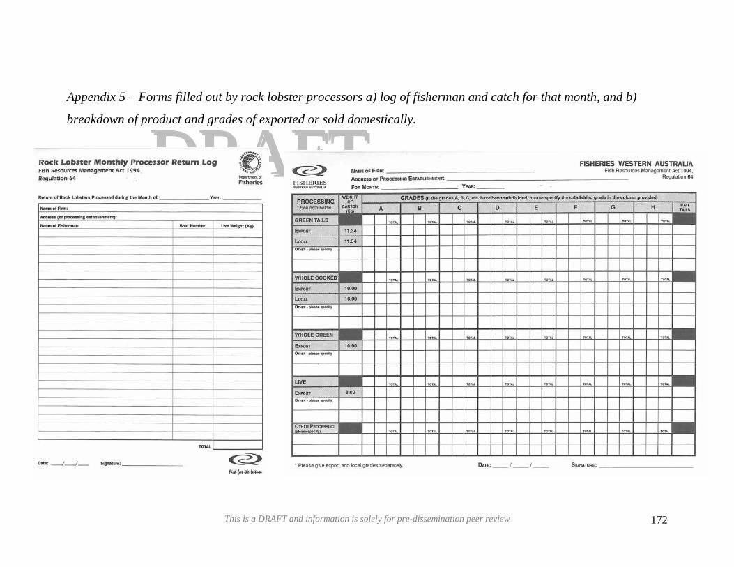
DDRRAAFFTTAppendix 5 – Forms filled out by rock lobster processors a) log of fisherman and catch for that month, and b)
breakdown of product and grades of exported or sold domestically.
This is a DRAFT and information is solely for pre-dissemination peer review 172
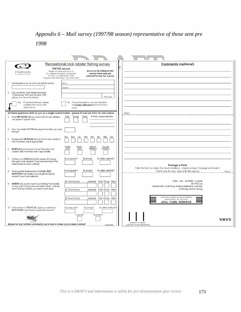
DDRRAAFFTTAppendix 6 – Mail survey (1997/98 season) representative of those sent pre
1998
This is a DRAFT and information is solely for pre-dissemination peer review 173
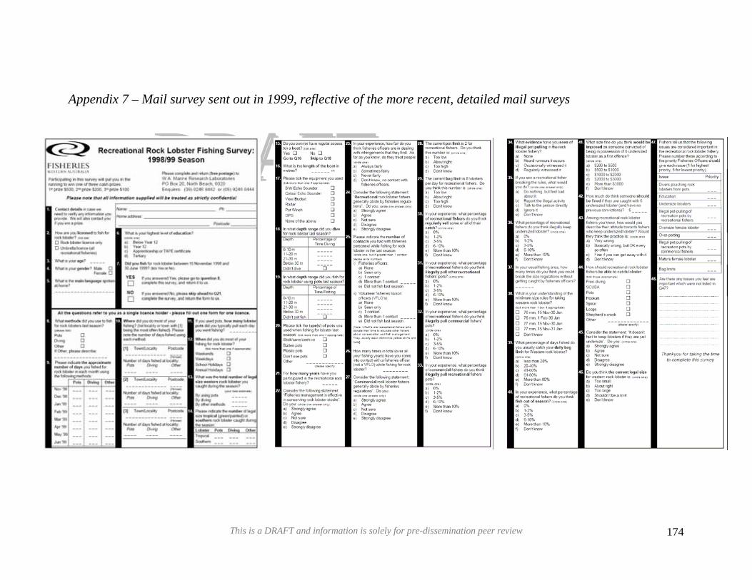
Appendix 7 – Mail survey sent out in 1999, reflective of the more recent, detailed mail surveys
DDRRAAFFTT
This is a DRAFT and information is solely for pre-dissemination peer review 174
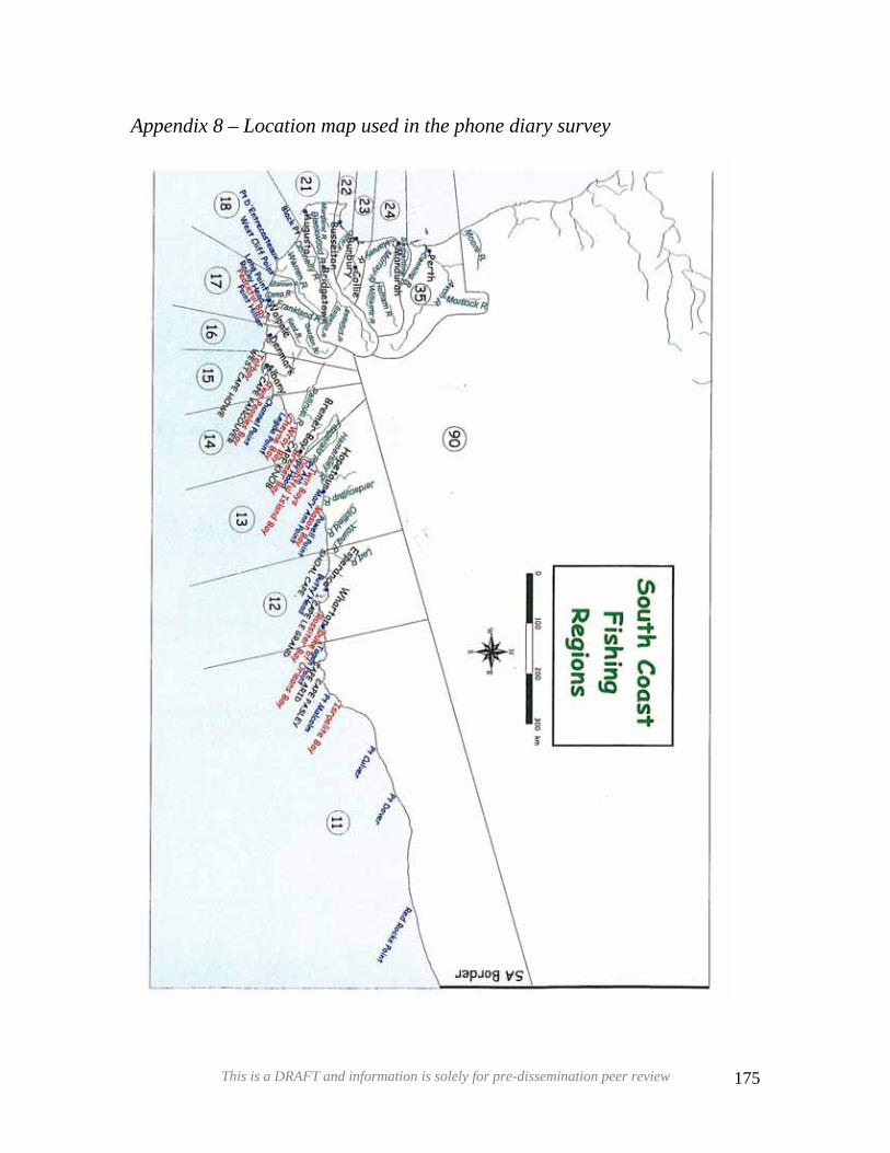
Appendix 8 – Location map used in the phone diary survey
DDRRAAFFTT
This is a DRAFT and information is solely for pre-dissemination peer review 175
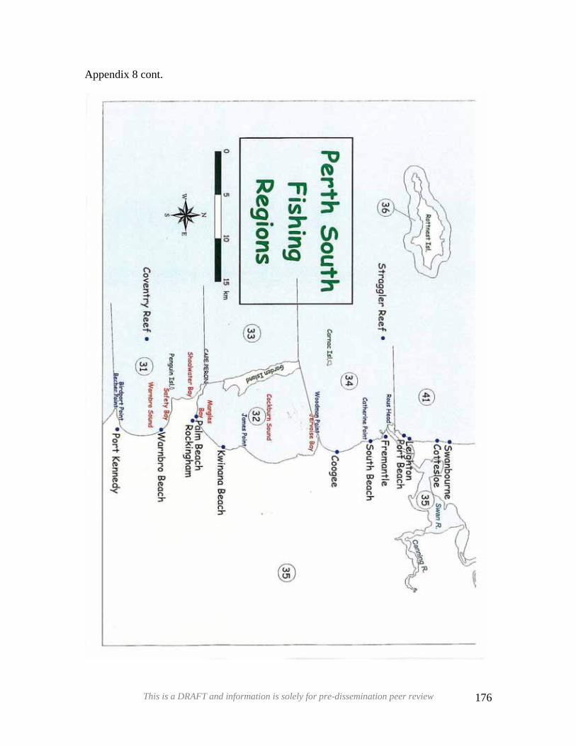
Appendix 8 cont.
DDRRAAFFTT
This is a DRAFT and information is solely for pre-dissemination peer review 176
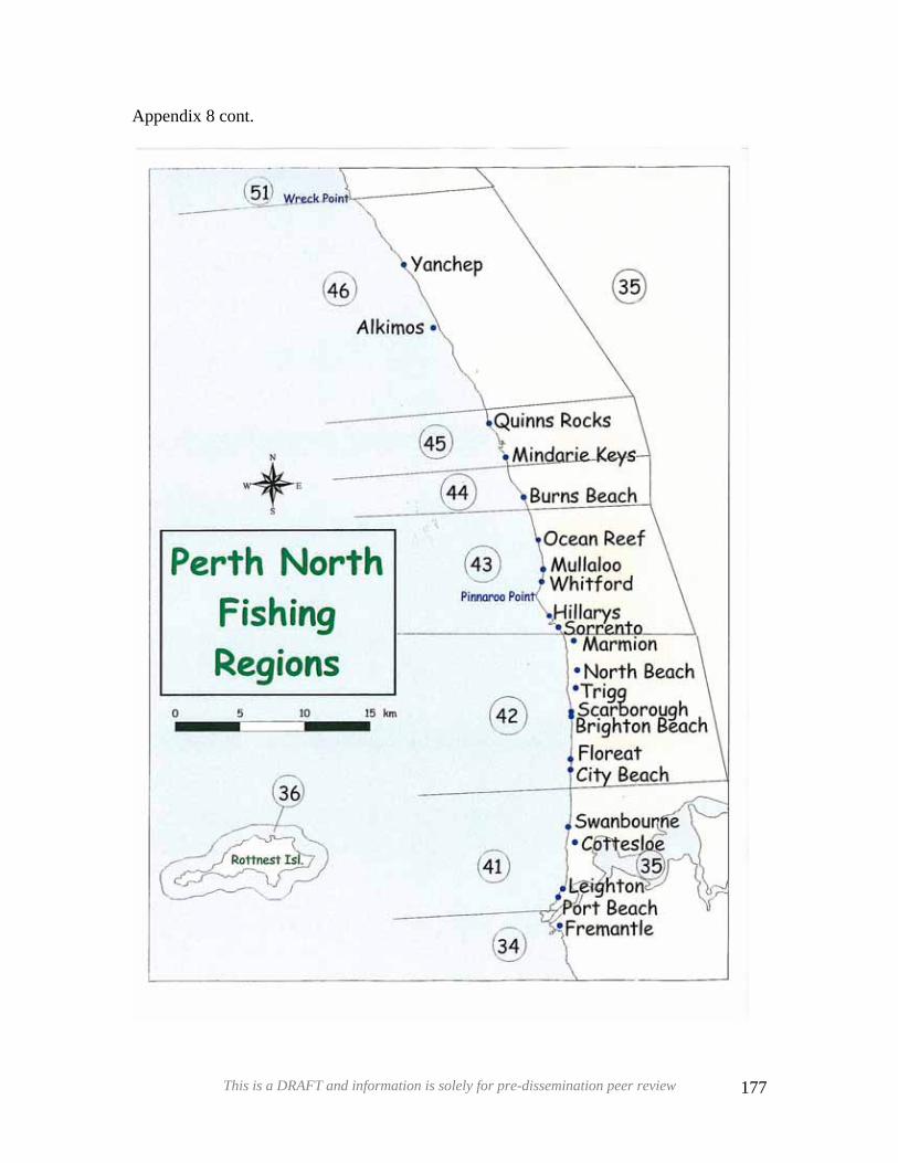
Appendix 8 cont.
DDRRAAFFTT
This is a DRAFT and information is solely for pre-dissemination peer review 177
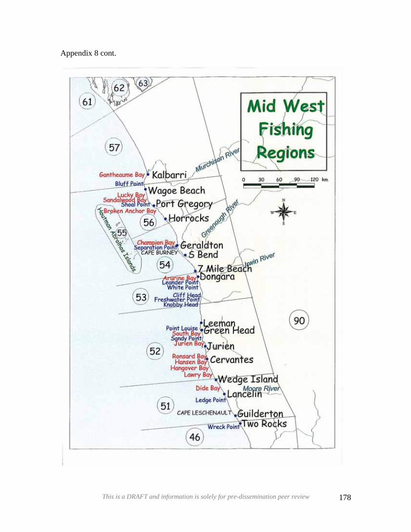
Appendix 8 cont.
DDRRAAFFTT
This is a DRAFT and information is solely for pre-dissemination peer review 178
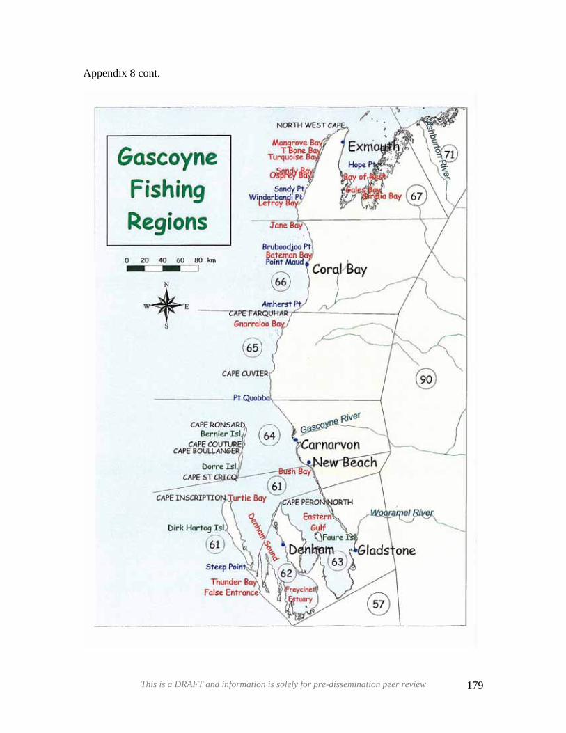
Appendix 8 cont.
DDRRAAFFTT
This is a DRAFT and information is solely for pre-dissemination peer review 179
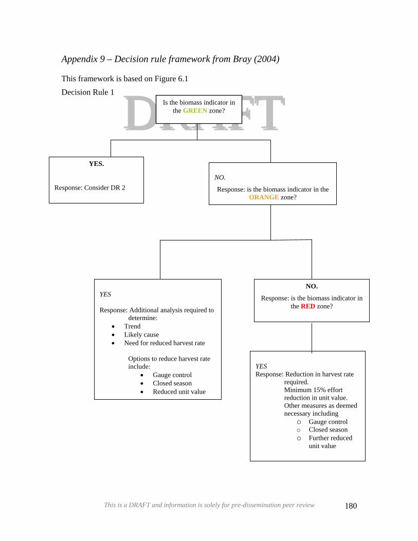
Appendix 9 – Decision rule framework from Bray (2004)
DDRRAAFFTTThis framework is based on Figure 6.1
Decision Rule 1
YES.
Response: Consider DR 2
YES
Response: Additional analysis required todetermine:
• Trend • Likely cause • Need for reduced harvest rate
Options to reduce harvest rate
include: • Gauge control • Closed season • Reduced unit value
Is the biomass indicator in the GREEN zone?
This is a DRAFT and information is sol
NO.
Response: is the biomass indicator in theORANGE zone?
NO.
Response: is the biomass indicator in the RED zone?
YES Response: Reduction in harvest rate
required. Minimum 15% effort
reduction in unit value. Other measures as deemed
necessary including o Gauge control o Closed season o Further reduced
unit value
ely for pre-dissemination peer review 180
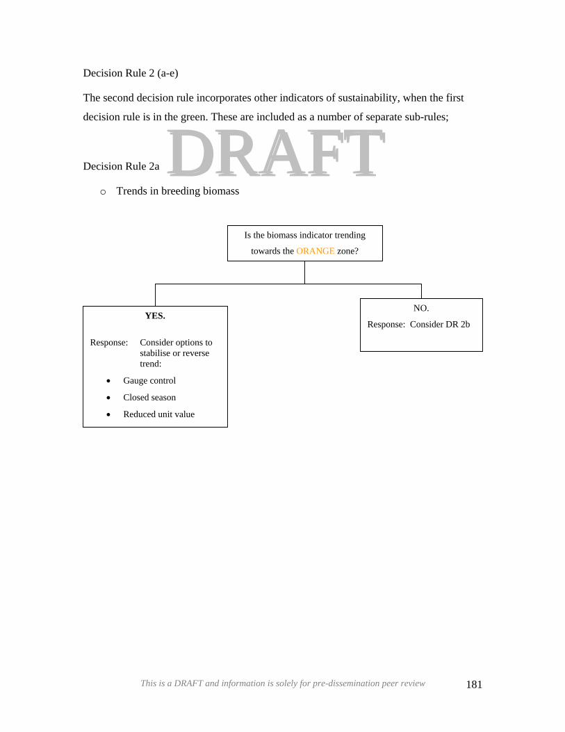
Decision Rule 2 (a-e)
DDRRAAFFTTThe second decision rule incorporates other indicators of sustainability, when the first
decision rule is in the green. These are included as a number of separate sub-rules;
Decision Rule 2a
o Trends in breeding biomass
Response: Cst
• Gaug
• Close
• Redu
This is a DRAFT and infor
Is the biomass indicator trending
towards the ORANGE zone?
NO.
Response: Consider DR 2b
YES.
onsider options to tabilise or reverse rend:
e control
d season
ced unit value
mation is solely for pre-dissemination peer review 181
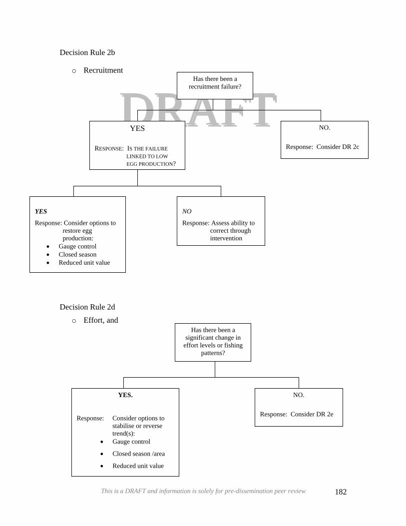
Decision Rule 2b
DD AAFFTTo Recruitment
RESPONSE:
LE
Response:
Has there been a recruitment failure?
Decision Rule 2d
o Effort, and
YE
Response: Consistabiltrend(
• Gaug
• Close
• Reduc
This is a D
RRYES
IS THE FAILURE INKED TO LOW GG PRODUCTION?
NO.
Response: Consider
S.
der options to ise or reverse s): e control
d season /area
ed unit value
Has there been a significant change in
effort levels or fishing patterns?
RAFT and information is solely for pre-dissemination peer review
NO.
Consider DR 2c
NO
Response: Assess ability to correct through intervention
YES
Response: Consider options to restore egg production:
• Gauge control • Closed season • Reduced unit value
DR 2e
182
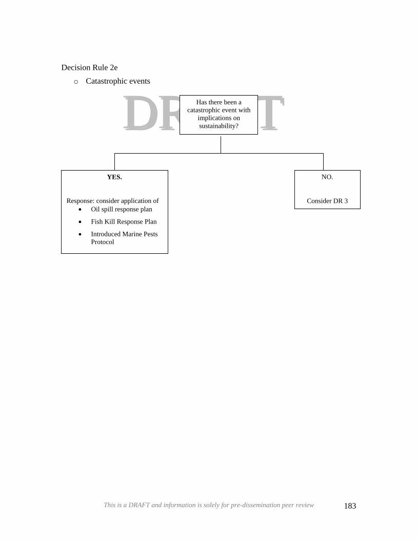
Decision Rule 2e
DDRRAAFFTTo Catastrophic events
NO.
Consider DR 3
YES.
Response: consider application of • Oil spill response plan
• Fish Kill Response Plan
• Introduced Marine Pests Protocol
Has there been a catastrophic event with
implications on sustainability?
This is a DRAFT and information is solely for pre-dissemination peer review 183
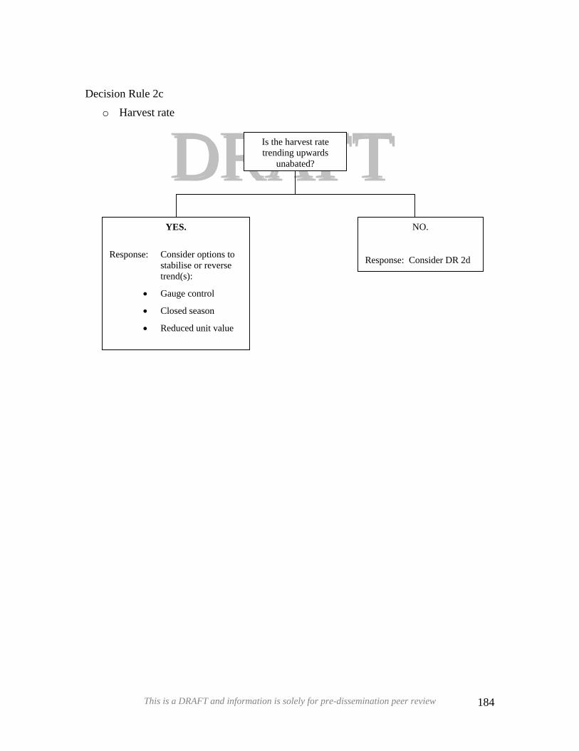
Decision Rule 2c
DDRR TTo Harvest rate
YES.
Response: Consider options to
stabilise or reverse trend(s):
• Gauge control
• Closed season
• Reduced unit value
This is a DRAFT and informat
AAFFIs the harvest rate trending upwards
unabated?
Response:
ion is solely for pre-dissemination peer
NO.
Consider DR 2d
review 184
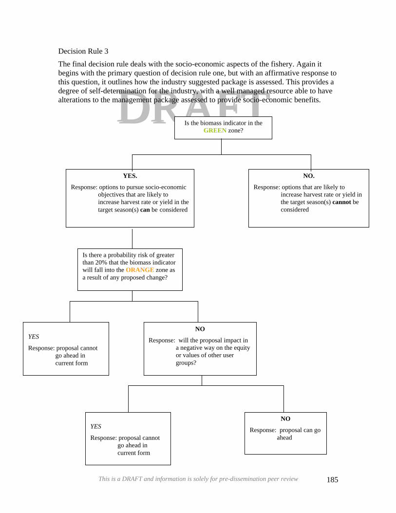
Decision Rule 3
DDRRAAFFTTThe final decision rule deals with the socio-economic aspects of the fishery. Again it begins with the primary question of decision rule one, but with an affirmative response to this question, it outlines how the industry suggested package is assessed. This provides a degree of self-determination for the industry, with a well managed resource able to have alterations to the management package assessed to provide socio-economic benefits.
YES.
Response: options to pursue socio-economic objectives that are likely to increase harvest rate or yield in the target season(s) can be considered
NO.
Response: options that are likely to increase harvest rate or yield in the target season(s) cannot be considered
YES
Response: proposal cannot go ahead in current form
NO
Response: will the proposal impact in a negative way on the equity or values of other user groups?
NO
Response: proposal can go ahead
YES
Response: proposal cannot go ahead in current form
Is there a probability risk of greater than 20% that the biomass indicator will fall into the ORANGE zone as a result of any proposed change?
Is the biomass indicator in the GREEN zone?
This is a DRAFT and information is solely for pre-dissemination peer review 185
Recommended