Luxembourg Income StudyWorking Paper No. 243
Explaining the Gender Poverty Gapin Developed and Transitional
Economies
Stephen Pressman
September 2000
EXPLAINING THE GENDER POVERTY GAP IN DEVELOPED AND TRANSITIONALECONOMIES*
Steven PressmanDepartment of Economics and Finance
Monmouth UniversityWest Long Branch, NJ 07764
(732) [email protected]
*An earlier version of this paper was presented at sessions of the2000 Review of Political Economy conference and the 2000 WorldConference of Social Economists. The author thanks theparticipants at these sessions for their helpful comments. Theusual caveat applies.
EXPLAINING THE GENDER POVERTY GAP IN DEVELOPED ANDTRANSITIONAL ECONOMIES
I. INTRODUCTION
As economies throughout the world experience large and
wrenching changes, poverty has increasingly become a problem
in country after country. This is true regardless of whether
these changes result from globalization, the economic
transition from socialism to capitalism, increasing
marketization and privatization, or some other major economic
transformation (Aslanbeigui, Pressman & Summerfield 1994; Funk
& Mueller 1993; Moghadam 1996).
A concomitant, disturbing aspect of rising poverty
throughout the world is that poverty has increasingly become
feminized-- women are much more likely than men to be poor.
This phenomenon was first noticed in the US (Pearce 1978,
1989; Pressman 1988), but more recently the problem of the
feminization of poverty has become an international concern as
well (Pressman 1998; Casper, McLanahan & Garfinkel 1994).
This article employs the Luxembourg Income Study (LIS) to
compare poverty rates for female-headed households (FHHs) with
poverty rates for other households in a number of developed
and transitional economies. It then seeks to explain why, in
some countries, female-headed households are so much more
likely to be poor compared to other families.
The next two sections describe the LIS and discuss some
of the problems encountered in measuring poverty. The paper
then computes poverty rates in individual countries for
2
female-headed households and for all other households using
the LIS database. Given the problems associated with
measuring poverty, we present several estimates of poverty for
both types of household. Two sections then look at two
theoretical explanations for the gender poverty gap-- human
capital theory and a Keynesian approach that emphasizes the
importance of fiscal policy as an antipoverty tool. The last
section summarizes the main findings and draws some policy
conclusions.
II. THE LUXEMBOURG INCOME STUDY
The Luxembourg Income Study began in April 1983 when the
government of Luxembourg agreed to develop, and make available
to social scientists, an international microdata set
containing a large number of income and socio-demographic
variables.
One goal in creating this database was to employ common
definitions and concepts so that variables are measured
according to uniform standards across countries. As a result,
researchers can be confident that the cross-national data they
are looking at and analyzing has been made as comparable as
possible.
By early 2000, the LIS contained information on 27
nations. Data for each country was originally derived from
national household surveys similar to the US Current
Population Reports, or from tax returns filed with the
national revenue service. Datasets for additional countries
3
are in the process of being added to the LIS.
Currently there are four waves of data available for
individual countries. Wave I contains datasets for the late
1970s and early 1980s. Wave II contains datasets for the mid
1980s. Wave III contains datasets for the late 1980s and
early 1990s. Finally, Wave IV (currently in the process of
being put online) contains country datasets for the mid 1990s.
LIS data is available for more than 100 income variables
and nearly 100 socio-demographic variables. Wage and salary
incomes are contained in the database for households as well
as for different household members. In addition, the dataset
includes information on in-kind earnings, property income,
alimony and child support, pension income, employer social
insurance contributions, and numerous government transfer
payments and in-kind benefits such as child allowances, Food
Stamps and social security. There is also information on five
different tax payments. Demographic variables are available
for factors such as the education level of household members;
the industries and occupations where adults in the family are
employed; the ages of all family members; household size,
ethnicity and race; and the marital status of the family or
household head.
This wealth of information permits researchers to do
cross-national studies of poverty and income distribution, and
to address empirically questions about the causes of poverty.
It also allows great flexibility in how income and poverty
4
are measured.
III. POVERTY CALCULATIONS USING THE LIS
How to calculate poverty rates has been a matter of
considerable controversy in the US since the 1960s. The
method currently employed was developed by Mollie Orshansky
(1965, 1969) of the Social Security Administration in the
early 1960s. Orshansky first calculated the cost of the
minimum amount of food that different types of families would
need during one year. Since Agriculture Department surveys
found that families spent around one-third of their after-tax
income on food, the cost of an economy food plan for families
of different types and sizes was multiplied by 3 in order to
arrive at poverty lines for each family type. Poverty lines
for each type of family are increased annually with the
increase in consumer prices. Poverty lines thus represent a
real standard of living for families of a particular type and
size that remains invariant over time. The poverty rate is
calculated as the percentage of US families whose income,
before taxes, falls below the poverty line (for their family
size and type) in a given year.
The Orshansky methodology for computing poverty rates has
been criticized on a number of grounds. Rodgers (2000) argues
that the minimum food requirements for a family were designed
for short-term emergency situations only and would not be able
to meet the nutritional needs of a family for an entire year.
Since the food budgets used by Orshansky were 80 percent of
5
what was necessary to provide a nutritional diet for the
entire year, Rodgers argues that the Orshansky poverty lines
are 80 percent too low. Schwarz and Volgy (1992) argue that
food consumption has fallen from one-third to one-fifth of
family spending, so current poverty lines should be based upon
a food multiplier of 5 rather than 3. This would raise
poverty lines by two-thirds, and also make poverty-level
incomes consistent with what public opinion surveys have found
to be the amount of income people believe that a family
requires to escape poverty. Taking a slightly different tack,
Watts (1986) argues that in the early 1960s the poor paid no
income taxes and virtually no social security taxes. But in
the 1970s and 1980s, poor families faced a considerable tax
burden. Calculating poverty based upon pre-tax incomes
ignores the fact that pre-tax incomes can buy less than a
comparable or real pre-tax income from the 1960s. Although
this point was undoubtedly a good one during the late 1980s,
it may no longer be valid given sharp increases in the earned
income tax credit during the 1990s.
The most frequent criticism of the Orshansky methodology,
however, is a philosophical one rather than a technical one.
Orshansky developed an absolute measure of poverty. Poverty
is supposed to measure the minimum income necessary for a
family to survive during the course of a year. But several
authors (Dunlop 1965, Fuchs 1965, Rainwater 1974, Ruggles
1990) have argued that human beings are social animals, and so
6
the standard of what is minimally necessary must vary from
time to time and from place to place. For example, private
baths and television sets were not necessities in the 1920s or
the 1930s, but they are necessities today. Likewise, child
care was not a necessity in the 1950s or 1960s. But as more
and more families have two earners, or just one adult heading
the household, child care becomes an important family
expenditure. For this reason, these authors contend that
poverty should be measured in relative terms, as some fraction
of the average income at a particular time and in a particular
place.
Additional problems arise when employing real, absolute
poverty lines in cross-national studies. Whenever we compare
two countries with different national currencies we have to
compare incomes that are measured in different units.
Consequently, some way has to be found to convert one income
into an equivalent income denominated in some other currency.
Exchange rates between two currencies is a first, logical
suggestion. But exchange rates vary considerably from day to
day, from month to month, and from year to year; and they vary
for speculative reasons that have nothing to do with changes
in the relative value of the two currencies or the relative
living standards in the two countries.
One attempt to get around this problem is to look at
purchasing power parity. The idea behind this notion is
straight-forward. Some goods are sold virtually everywhere
7
throughout the world; by comparing the cost of these goods
from country to country we can obtain a good measure of the
real value of two different currencies. If a McDonald's
hamburger sells for $1 in the United States and 100 yen in
Japan, then $1 and 100 yen should represent equivalent real
incomes. According to the purchasing power parity theory,
regardless of the exchange rate between the dollar and the
yen, $1=100 yen should be used when comparing real incomes in
the US and Japan.
Unfortunately, serious problems with the notion of
purchasing power parity make its use problematic when
attempting to compare equivalent incomes in different nations.
Purchasing power parity assumes that domestic prices for any
good reflect only domestic costs. Transportation costs and
other costs of trade as well, as all trade restrictions, get
assumed away. So, too, do the different spending patterns
that exist in different countries. In the real world,
however, these factors are all important in determining the
price of goods in a particular country.
Because of the arguments in favor of a relative notion of
poverty, and because of problems with comparing real incomes
across nations, most LIS studies have employed a relative
notion of poverty. These studies usually define poverty lines
as 50 percent of median adjusted family or household income,
after taxes, within a country for a specified year. Adjusted
family income controls for the different sizes of different
8
families, and recognizes that $20,000 goes a lot further in a
family of 2 than in a family of 5. Most empirical studies
using the LIS take the income needs of a second adult to be 70
percent of the income needs of a first adult and the income
needs of children as 50 percent of the first adult. These
weights are similar to the implicit weights in the official US
definition of poverty, and the family equivalence scales used
by the OECD.
IV. ESTIMATING THE GENDER POVERTY GAP
Following the standard LIS methodology for computing
poverty, Table 1 presents poverty rates for those countries in
Wave III of the LIS. Poverty rates are calculated for
households headed by a single female and also for all other
households. The last column of each table shows the
difference between the poverty rate for female-headed
households and the poverty rate for all other households.
For Wave III, the difference between these two poverty
rates (the gender poverty gap) ranges from around -2%, (for
Poland), meaning that poverty rates for female-headed
households are two percentage points lower than other poverty
rates for other families, to about +18% (for the US), meaning
that poverty rates for female-headed US households are 18
percentage points higher than poverty rates for other US
households. For Wave III datasets, the gender poverty gap
averages 4.4% (unweighted).
A number of studies of the poverty gap (e.g., Casper,
9
McLanahan & Garfinkel 1994; Christopher et al. 1999) have
looked at the ratio of poverty rates for female-headed
households and other households rather than differences in
these two rates. This approach may result from the habits of
labor economists, who typically examine and study earnings
ratios. But looking at poverty rate ratios is objectionable
on two counts. First, poverty rates are supposed to represent
the probability that a family is poor. When comparing the
poverty rate for female-headed households with the poverty
rate for other households we usually want to know how much
more likely it is that female-headed household will be poor.
Differences in poverty rates give us this important
information; ratios do not.
Second, with ratios, small percentage point differences
can lead to large ratio differences that can be misleading
when we attempt to interpret the numbers or analyze the causes
of the gender poverty gap. For example, if 1% of other
households are calculated to be poor and 2% of female-headed
households are poor (essentially the results for the Czech
Republic), ratios focus on the fact that women are twice as
likely to be poor as men. But given the reporting errors in
survey data, plus the somewhat arbitrary nature of any
equivalence scales and poverty lines, the difference between a
poverty rate of 1% and a poverty rate of 2% is quite small and
may not be robust or significant. Differences in poverty
rates makes this fact clear; poverty rate ratios do not. To
10
the contrary, with ratios, a poverty rate for female-headed
households of 20% and a poverty rate for other households of
10% (essentially the case of Canada) seem just as bad as the
2% and 1% case because it also yields a ratio of 2. But
clearly, women in the Czech Republic are relatively better off
than the women in Canada. To make this clear it is necessary
to focus on poverty rate differences rather than on ratios of
poverty rates.
The gender poverty gaps reported in Table 1 divide
naturally into three different groups. First, there are
countries with very small and insignificant gender poverty
gaps. For Belgium (1992), the Czech Republic, Hungary, Italy,
Luxembourg, the Slovak Republic and Spain there is virtually
no difference between poverty rates for female-headed
households and for other households; and in two countries
(Poland and Switzerland) poverty rates for female-headed
households are slightly below poverty rates for other
households. Second, 11 countries (Belgium (1988), Denmark,
Finland, France, Germany, Israel, the Netherlands, Norway,
Sweden, Taiwan, and the UK) have slightly higher FHH poverty
rates. For these countries the gender poverty gap ranges from
around 2 percentage points (Norway) to a little more than 6
percentage points (United Kingdom). Finally, four countries
have extremely large gender poverty gaps. In Canada, the
gender poverty gap is almost 10 percentage points; and in
Australia, the gender poverty gap exceeds 11 percentage
11
points. Even worse performers are Russia, with a gender
poverty gap of almost 15 percentage points and the United
States where the gender poverty gap approaches 18 percentage
points.
Studies using other waves of the LIS, and examining
female-headed households and poverty (Wright 1995; Pressman
1998), have found a similar pattern. Those countries with a
small gender poverty gap in one year tend to have a small
gender poverty gap in the other year. Australia, Canada and
the US do badly in both time periods (there is no Russian
database for Wave II); while Italy, Luxembourg and Poland do
well in both time periods. Countries falling in the middle
ground in one time period also tend to fall in the middle
ground in other time periods. There thus appears to be
relatively little change from one wave or time period to the
next when it comes to rank ordering countries. Put another
way, international differences in poverty are much greater in
one time period than intertemporal differences in poverty in
one nation.
One interesting question is what has happened in
transitional economies as a result of sharp reductions in the
role of government in economic activity and giving greater
sway to the market. Wave II datasets provide a benchmark for
before the transition process; Wave III datasets give a
snapshot of the very beginning of the transformation process.
These Waves show only small gender poverty gaps. When Waves
12
IV and V datasets finally come online we will be able to see
the impact of the full transition process. Other evidence of
the impact of this transformation on women (Funk & Mueller
1993; Aslanbeigui, Pressman & Summerfield 1994) prevents one
from being optimistic about gender poverty gaps for these
nations as the transition process moves forward.
V. A SENSITIVITY ANALYSIS
Given the problems with survey data, as well the problems
with defining poverty that we discussed in section III, one
important question that needs to be addressed is how much
hinges on the decisions that get made when measuring poverty.
This section attempts to answer this question by means of a
sensitivity analysis.
Table 2 uses Wave III of the LIS and the standard
equivalence scales for deriving adjusted family income. It
differs only by using a slightly different definition of
poverty. In Table 2, households are taken to be poor if the
family income falls below 40% of mean adjusted household
income (rather than the usual 50%). Using this alternative
poverty definition the stylized facts presented in section IV
do not change very much. The US still has the greatest
problem of feminized poverty, although the poverty rate for
FHHs and the gender poverty gap are both a bit lower due to
the lower poverty line. Moreover, the same four countries
(Australia, Canada, Russia and the US) still have the largest
gender poverty gaps and the highest poverty rates for FHHs.
13
Likewise, most of the countries with low gender poverty gaps
using a 50% of median income poverty line also have low or no
gender poverty gaps when defining poverty as having less than
40% of adjusted mean family income. Poland has the lowest
gender poverty gap in both instances. And the same set of
countries (the Czech Republic, Hungary, Italy, Luxembourg, the
Slovak Republic, Spain and Switzerland) have negligible gender
poverty gaps in both time periods. The only major change in
our results is that a number of countries with moderate gender
poverty gaps when we set a higher poverty line now have
negligible poverty gaps. In the UK, for example, the gender
poverty gap falls from 6.3% to 0.1%, while in Israel the
gender poverty gap falls from 4.8% to 0.9%. Overall, the
correlation between the gender poverty gap using a poverty
line set at 50% of median (adjusted) income and the gender
poverty gap using a poverty line set at 40% of median
(adjusted) income exceeds 80 percent.
Table 3 uses Wave III LIS datasets as well as the
standard LIS poverty line-- 50% of median adjusted household
income. However, it differs from Table 1 by using a different
equivalence scale to get adjusted household incomes. Table 3
gives every person in a given household an equal weight,
thereby assuming that no economies of scale exist for
household consumption. We can think of this as the other
extreme to the normal assumption of fairly significant
economies of scale in family size.
14
This change also does not seem to have much impact on our
story about women and poverty. The main change here is that
poverty rates are higher when we assume that each child has
the same income needs as the first adult in the family (rather
than needs that are one-half of that). This pushes down
adjusted household income and many more households with
children are categorized as poor. Since female-headed
households typically have more children than other households
(because married couples without children are all counted as
part of other households), we get higher gender poverty gaps
when we look at per capita household incomes.
Nonetheless, the trans-national story about women and
poverty changes very little with our alternative measure of
household income. Again, the US has the largest gender
poverty gap of all countries examined as well as the highest
poverty rate for FHHs. Likewise, the same set of four
countries (Australia, Canada, Russia and the US) still have
the largest gender poverty gaps and the four highest poverty
rates for FHHs. At the other end of the spectrum, Poland
continues to have the lowest (negative) gender poverty gap,
while the same set of countries generally tend to have the low
gaps. The correlation between the gender poverty gap
estimated in Table 1 and the gender poverty gap on this
alternative definition of adjusted household income is 70
percent.
VI. POSSIBLE CAUSES OF THE GENDER POVERTY GAP
15
Theoretical explanations for different gender poverty
gaps among nations can generally be divided into three broad
categories.
First, neoclassical economic theory attributes wage
differentials primarily to productivity differences. Someone
who is more valuable to their firm will get paid more than
someone who contributes less to firm revenues. Human capital
theory (Becker 1993) has taken this idea one step further, and
has attempted to explain wage rates based upon the education
and experience level of the individual. The insight of human
capital theory is that more educated workers will be more
productive and will thus receive higher pay. Likewise, more
experienced workers will be more productive, and should also
be paid more money than less experienced workers.
This theory can be applied to gender differences in
earnings. If the education level of women who head up
households is much less than the education level of men who
head up married-couple families, we should expect the earnings
and income of female-headed households to be much lower.
Therefore, we should expect the gender poverty gap to be
larger. Human capital theory traditionally proxies experience
by looking at the age of the individual worker. Adopting this
approach, we can look towards the age of household heads in
order to explain the gender poverty gap. If female heads of
house are younger than the men who head up other households,
then according to human capital theory the wages of these
16
women should be lower than the wages of the men heading up
other families. Again, with lower relative wages, women
should experience relatively greater poverty.
A second possible explanation for gender poverty gaps
focuses on gender discrimination. Societal views about the
worth of women and the work they do have led to a situation
where women receive lower pay than men, even when they do the
same work and provide the same benefits to the firm. Another
take on the discrimination angle is the claim that
occupational sex segregation has put women into a set of jobs
with low pay (Bergmann 1974, Sawhill 1976, Strober & Arnold
1987) or a set of industries (the service sector) that pay
poorly (Northrop 1990). Obviously, the greater the
discrimination against women in the marketplace, the lower the
earnings of women relative to men and the higher the gender
poverty gap will be.
Finally, government fiscal policies can affect the gender
poverty gap in two main ways. Within a particular country,
spending programs, or social transfer payments, can be geared
more towards husband-wife households or more towards female-
headed households. The more that social programs give to
female-headed households relative to other households, the
lower the gender poverty gap should be. Meager social
insurance for female-headed families in the US has been cited
(Rodgers 2000, Zopf 1989) as a major cause of high poverty
rates for female-headed households. This factor also may
17
contribute to different national gender poverty gaps.
In addition to spending money, governments also collect
taxes. Poverty calculations are usually made using after-tax,
rather than before-tax, incomes. If government tax policy in
one country favors married-couple households over single tax-
paying units, female-headed households will do relatively
worse after-taxes than other households, and we should see a
greater gender poverty gap.
VII. TESTING ALTERNATIVE THEORIES OF THE GENDER POVERTY GAP
This section examines two of the three theories discussed
above. We first explore how human capital considerations
affect the gender poverty gap. Then we look at the impact of
fiscal policy on the gender poverty gap. Given the usual time
and space constraints, tests of the feminist approach, which
look to discrimination as the cause of the gender poverty gap,
will be left for future research.
Table 4 examines one part of the human capital
explanation for the gender poverty gap. It raises the
following empirical question-- to what extent is the poverty
of female-headed households due to the relative youth of the
household head? To answer this question we take poverty rates
as a weighted average of the poverty experienced by households
whose heads fall into different age brackets. To derive the
figures appearing in Table 5, six different age groups were
distinguished-- (1) under 30, (2) 31-39, (3) 40-49, (4) 50-59,
(5) 60-69, and (6) over 70. For most countries, especially
18
for developed countries, this results in six groups of
relatively equal size for other households. Poverty rates for
each age group were calculated for both FHHs and other
households in each individual country. Table 4 recalculates
poverty rates for FHHs as the weighted average of the
(constant) poverty rates for each age group, assuming that
female-headed households had the same age distribution as
other households. The results of this computation are shown
in column 3. Column 4 shows the change in poverty for FHHs in
each country due to the age distribution of female household
heads.
This exercise does not lend a great deal of support to
the human capital explanation for the gender poverty gap. Of
the 23 countries for which it was possible to calculate
poverty rates by the age and gender of household head, in 15
instances poverty for female-headed households was lower due
to their actual age distribution. In only 8 out of 23 cases
(a bit more than 33%) did the relative youth of female-headed
households increase their likelihood of being poor. Moreover,
in only one instance (Russia) were poverty rates for FHHs
substantially higher due to the age distribution of FHHs. On
average (unweighted), poverty rates of FHHs were one-tenth of
a percentage point lower as a result of the age distribution
of FHHs. This is not significantly different from zero, and
so age cannot explain the gender poverty gap of Table 1.
One reason age is unimportant is that in many countries
19
FHHs are more likely to have older heads due to the greater
life expectancy of women. Moreover, older households are less
likely to be poor due to the generous provision of retirement
income to the elderly.
To take just one striking example we consider the
Australian (1989) case. Younger FHHs (under 40) had around a
28% chance of being poor. In contrast, only around 15% of
middle-aged FHHs (40-59) were poor and less than 10% of FHHs
with an elderly head (60+) were poor. Since women live longer
than men, there are proportionately more older FHHs than older
other households in Australia. Around 21% of other households
are 60 and over, but more than 36% of FHHs were 60 and over.
The fact that FHHs are more likely to be older reduced the
poverty of FHHs by around 1.3 percentage points in Australia.
If FHHs had the same age distribution as other households,
their poverty rate would have been 20.5% (rather than the
actual 19.1%).
Table 5 looks at the other part of the human capital
explanation for the gender poverty gap. It address the extent
to which the poverty of FHHs is due to their lower levels of
education. As noted above, we can regard poverty rates for
FHHs as a weighted average of the poverty experienced by
families with different characteristics. Here the relevant
feature is educational levels rather than age.
The LIS does not have standard educational achievement
classifications that are used in all country databases. But
20
for each country, education categories are pretty much defined
the same way for FHHs and for other households. In those few
instances where categories were not identical, some minor
recoding was needed. In these cases, only a very small
percentage of households (less than one-half of one percent)
had to be recoded, so recoding decisions will not affect the
overall results. In a couple of cases (Israel and the United
Kingdom) education data was available only by the age at which
the individual last attended school; since this was not likely
to be a very close proxy for educational attainment, these
countries were excluded from Table 5. For Russia, the
recoding task was too large (since educational attainment
categories differ substantially by gender) and would likely
affect the final results because of the large number (30) of
education categories in the Russian LIS database. For this
reason, Russia was excluded from the analysis of education and
the gender poverty gap in Table 5.
Column 3 of Table 5 shows the poverty rates for FHHs
under the assumption that they had the same educational
distribution as other household heads. Column 4 of Table 5
then shows the increase in poverty for FHHs that is due to the
lower educational attainment of the household head.
Again the results do not lend much support to the human
capital explanation for the gender poverty gap. In 8 cases
out of 20 (Belgium, Denmark, France, the Netherlands, Norway,
the Slovak Republic, Sweden and Switzerland), FHHs actually
21
were less likely to be poor because of their education. In
three more cases (the Czech Republic, Finland and Luxembourg),
educational attainment made virtually no difference at all.
In contrast, for only 6 countries (Germany, Hungary, Italy,
Poland, Spain, and the US) did educational deficiencies raise
the poverty rate of FHH by more than 1 percentage point, and
in only one of these (the US) did it raise the poverty rate of
FHH by more than 2 percentage points. The striking result of
Table 5 is that educational levels matter very little. On
average (unweighted), lower education levels for women raised
the poverty rate of FHH by one-half of a percentage point.
Consequently, educational deficiencies by women can explain
only a little more than 10% of the gender poverty gap that we
estimated in Table 1.
While human capital theory does not help explain the
gender poverty gap, Keynesian theory does considerably better.
The Keynesian argument is that income distribution in
general, and poverty rates in specific, depend on fiscal
policy decisions made by the government. On the Keynesian
view, the bigger the government safety net, and the broader
and deeper (or more generous) the net, the lower the national
poverty rate (see Pressman 1991). Because FHHs are more
likely to be poor without any government assistance, the more
generous the level of government transfer payments, lower the
gender poverty gap.
Tables 6, 7 and 8 allow us to examine this theory. Table
22
6 assumes no government benefits and that no taxes are imposed
on earned incomes. It also assumes that there are no private
transfers among households, such as child support or alimony
payments. As a result, factor income (wages, interest,
dividends, rent, etc.) is taken to be total household income.
Calculating poverty analogous to our method in Table 1-- not
receiving at least 50% of median (adjusted) household factor
income-- gives us enormously high poverty rates. This is
especially so for FHHs, where poverty rates typically exceed
50% and reach as high as 70%. This, no doubt, stems from the
fact that FHHs usually have only a single adult earner. When
women head up families with children, they may have child
rearing responsibilities that limit the number of hours they
can work each day and each week, and therefore the sorts of
jobs they could hold. Moreover, women typically earn less
than men, and so they suffer a further disadvantage. The
result is that FHHs have low factor incomes and high poverty
rates compared to other households.
The gender poverty gap in Table 6 is rather striking; it
averages (unweighted) more than 30% when fiscal policy and
private transfers are excluded. This contrasts with an
average poverty gap of 4.4% when taking the impact of
government spending and taxes as well as private transfers
into account (Table 1). Also striking is the fact that when
we look at just factor incomes, the US gender poverty gap lies
a bit below the (unweighted) average gender poverty gap for
23
all countries in Table 6. Likewise, the poverty rate of FHHs
in the US is below the (unweighted) average for all LIS
countries in Wave III. What is true of the US is also true of
Canada and Russia, two of the other four countries with very
high gender poverty gaps. Looking at only factor incomes,
both have below average poverty rates for FHHs and below
average gender poverty gaps. Canada, in fact, has the second
lowest gender poverty gap and the third lowest poverty rte for
FHHs when looking at just factor income. Australia, our last
poorly performing country, has a below average poverty rate
for FHHs, but a gender poverty gap that is slightly above
average.
Overall, Table 6 makes it quite clear that measured in
terms of income received from economic activity, women do
rather badly in one country after the next. Ignoring all
private transfers and fiscal policy, in nearly every country
FHHs would stand a greater than 50% chance of being poor.
They would also be 32% more likely to be poor than other
households in virtually all countries.
Table 7 adds two important private transfers to factor
income-- child support and alimony payments. Poverty rates in
each country are again computed based on whether adjusted
household income falls below 50% of median adjusted household
income. The main result of Table 7 is that private transfers
seem to make very little difference. Adding these payments to
household income reduces poverty rates for FHHs a little and
24
reduces the gender poverty gap a bit (each goes down by half a
percentage point), but in both cases these rates remain very
high.
Table 8 looks at gross income before taxes. Here we
include all government benefits in family income figures as
well as all private transfers. Poverty rates again are
calculated as the fraction of families whose gross income
(adjusted for family size) falls below 50% of median
(adjusted) gross income. As before, the poverty gap is the
difference between the poverty rate for FHHs and the poverty
rate for other households.
The first striking thing about Table 8 is the sharp drop
in poverty due to various government transfer payments.
Government expenditures reduce the poverty rate of FHHs by
around two-thirds and also reduce the poverty rate of other
households by around two-thirds.
These declines, it is important to note, are not the
result of just adding more types of income (and therefore more
income) to each household. Poverty rates are computed based
on a poverty line that is 50% of (adjusted) gross income;
since gross income exceeds factor income for each family,
median income rises for every family and the poverty line
rises as well. In fact, if gross income rose proportionately
to factor income for every household, there would be no change
in poverty rates at all. So the sharp decline in poverty that
we see in Table 8 must be due to the equalizing effect of the
25
added government expenditures.
The second thing to notice about the last column of Table
8 is the sharp drop in the gender poverty gap. On average
(unweighted), government expenditures reduce the gap by nearly
24 percentage points-- from 30.7 percent to 7.2 percent-- or
by more than two-thirds. Moreover, there is a sharp drop in
the gender poverty gap in virtually every country. Among the
major exceptions here are the US, Australia, Canada and
Russia, where fiscal expenditures do relatively little to
lower the gender poverty gap. As a result, these countries
have gender poverty gaps of between 15 to 20 percent when
measured using (adjusted) family gross income.
Moving from the last column of Table 8 back to Table 1,
enables us to see the impact of taxes on poverty and the
gender poverty gap. On average (unweighted), the tax system
reduces the gender poverty rate for FHHs by 4.4 percentage
points and the poverty rate for other households by 1.5
percentage points. Thus the poverty gap falls by 2.8
percentage points due to taxes.
But taxes are not equally effective at mitigating the
poverty gap in all countries. In Australia, the poverty gap
is reduced by nearly 9 percentage points; however, Australia
still remains with a large poverty gap due to the
ineffectiveness of government expenditures in helping low
income FHFs. Similarly, in Denmark and Finland the gender
poverty gap falls by around 8 percentage points (from 13% to
26
5% and from 12.5% to 4.4%, respectively); but since government
expenditures are relatively ineffective in mitigating the
Danish and Finnish gender poverty gap, Denmark and Finland
still end up with moderately high gaps. In contrast, countries
like the Netherlands, Switzerland, France and Czech Republic
make little use of the tax system to equalize income and
thereby reduce poverty for FHHs. But since they make great
use of government expenditures to lower the gender poverty
gap, they all wind up with relatively low gender poverty gaps.
In the US, taxes reduce the poverty gap by 3.2 percentage
points, which is not that much above the (unweighted) average
for all the countries we have examined. But because the US
started with such a large gender poverty gap before taxes get
taken into account, taxes have little overall impact. What is
true of the US is also true of both Canada and Russia. For
all four countries with larger gender poverty gaps we see a
failure to use fiscal policy, especially government spending
programs, to buttress the incomes of those who make little
money through market activities.
Table 9 pulls together the results of our analysis in
this section. It starts where most families start, with
factor incomes, the money earned from market activities. Had
this been the only source of income for families, the gender
poverty gap would be nearly 30 percent in most countries, and
it would be quite invariant from country to country. Adding
private transfers (child support payments and alimony)
27
slightly lowers the gender poverty gap in virtually all
nations and slightly lowers it on average. Most of the action
in lowering the gender poverty gap, however, occurs as a
result of fiscal tax and transfer policies, especially the
latter. Countries that do the most for FHHs see the largest
reductions in the gender poverty gap; countries without a
fiscal policy that aids FHHs see little reduction from the
high gender poverty gaps that result when looking at only
factor incomes.
VIII. SUMMARY AND CONCLUSIONS
This paper has examined the gender poverty gap in a wide
set of countries using Wave III of the Luxembourg Income
Study. It finds that the gender poverty gap was relatively
large in some countries during the late 1980s and early 1990s,
was moderate in other countries, and was very low or negative
in yet other countries. These results were robust with
different attempts to measure poverty.
Next, the paper sought the causes of different gender
poverty gaps across countries. It found the human capital
explanation wanting. Neither age nor education can explain
much of the gender poverty gap. A more Keynesian explanation
for the gender poverty gap proved more fruitful. Fiscal
policy is able to explain a large proportion of the gap.
Excluding government, the poverty rate of FHHs and the gender
poverty gap are very large in all countries. Some nations use
fiscal policy aggressively to assist FHHs; other less so.
28
Those nations that do more have much lower poverty rates for
FHHs and much lower gender poverty gaps. In contrast, nations
like Australia, Canada, Russia and the US fail to employ
fiscal policy aggressively in an attempt to assist poor
families; as a result they wind up with large poverty rates.
These countries also do not focus their fiscal assistance on
FHHs and so these nations have high poverty rates for FHHs and
large gender poverty gaps. The results of this paper thus
support other studies which found that the type of welfare
state and the character of social policies and spending
programs affect poverty rates for single mothers (Duncan &
Edwards 1997; Lewis 1997).
This analysis also leads to two policy conclusions.
First, attempts to improve the economic condition of FHHs by
developing the skills and improving the education level of
women are not likely to be effective. Similarly, any sort of
welfare reform, which reduces government benefits and forces
women to work more, will likely exacerbate the problem of
women and poverty. Second, fiscal policy must focus more on
the problems facing FHHs and the impact of any spending or tax
changes on FHHs. If countries are to effectively deal with
problems of feminized poverty, then fiscal policy must be used
to assist FHHs.
REFERENCES
Aslanbeigui, N., Pressman, S., & Summerfield, G. (1994) Womenin The Age of Economic Transformation. New York & London:Routledge.
29
Becker, G. (1993) Human Capital, 3rd ed. Chicago: Universityof
Chicago Press.
Bergmann, B. (1974) "Occupational Segregation, Wages andProfits
When Employers Discriminate By Race/Sex," EasternEconomic
Journal, 1: 103-110.
Casper, L., McLanahan, S. & Garfinkel, I. (1994) "The Gender-Poverty Gap: What Can we Learn from Other Countries?,"American Sociological Review, 59: 594-605.
Christopher, K., England, P., Ross, K., Smeeding, T. &McLanahan, S. (1999) "The Sex Gap in Modern Nations:
SingleMotherhood, the Market, and the State," LIS Working
Paper.
Duncan, S. & Edwards, R. (1997) Single Mothers in anInternational Context. London: UCL Press.
Dunlop, J.T. (1965) "Poverty: Definition and Measurement" inThe
Concept of Poverty. Washington, DC: Chamber of Commerceof
the United States of America.
Fuchs, V.R. (1965) "Toward a Theory of Poverty" in The Conceptof Poverty. Washington, D.C.: Chamber of Commerce of theUnited States of America.
Fuchs, V.R. (1988) Women's Quest for Economic Equality.Cambridge: Harvard University Press.
Fuchs, N. & Mueller, M. (1993) Gender Politics and Post-Communism: Relfections from Eastern Europe and the FormerSoviet Union. New York: Routledge.
Funk, N. & Mueller, M. (1993) Gender Politics and Post-Communism:
Reflections from Eastern Europe and the Former SovietUnion. New York: Routledge.
Lewis, J. (Ed.)(1997) Lone Mothers in European WelfareRegimes.
London: Jessica Kingsley.
Moghadam, V. (1996) Patriarchy and Economic Development:Women's
Positions at the End of the Twentieth Century. New York:
30
Clarendon Press.
Northrop, E. (1990) "The Feminization of Poverty: TheDemographic
Factor and the Composition of Economic Growth," Journalof
Economic Issues, 24: 145-160.
Orshansky, M. (1965) "Consumption, Work, and Poverty" in B.B.Seligman (Ed.) Poverty as a Public Issue. New York: FreePress.
Orshansky, M. (1969) "How Poverty is Measured," Monthly LaborReview, 92: 37-41.
Pearce, D. (1978) "The Feminization of Poverty: Women, Workand
Welfare," Urban and Social Change Review, 11: 28-36.
Pearce, D.M. (1989) The Feminization of Poverty: A SecondLook.
Washington, D.C.: Institute for Women's Policy Research.
Pearce, D.M. & McAdoo, H. (1981) Women and Children: Alone inPoverty, Washington, D.C.: National Advisory Council onEconomic Opportunity.
Pressman, S. (1988) "The Feminization of Poverty: Causes andRemedies," Challenge, 31 (2): 57-61.
Pressman, S. (1991) "Keynes and Antipoverty Policy," Review ofSocial Economy, 49 (3): 365-82.
Pressman, S. (1998) "The Gender Poverty Gap in DevelopedCountries: Causes and Cures," Social Science Journal, 35(2): 275-286.
Rainwater, L. (1974) What Money Buys: Inequality and theSocial
Meaning of Income. New York: Basic Books.
Rodgers, H.R., Jr. (2000) American Poverty in a New Era ofReform
Armonk, NY: M.E. Sharpe.
Ruggles, P. (1990) Drawing the Line: Alternative PovertyMeasures
and Their Implications for Public Policy. Washington, DC:Urban Institute Press.
Sawhill, I. (1976) "Discrimination and Poverty Among Women-Headed
31
Families" in M. Blaxall and B. Reagan (Eds) Women and theWorkplace: The Implications of Occupational Segregation.Chicago: University of Chicago Press.
Schwarz, J.E. and Volgy, T.J. (1992) The Forgotten American.New
York: Norton.
Strober, M.H. and Arnold, C.L. (1987) "The Dynamics ofOccupational Segregation Among Bank Tellers," in C. Brownand J. A. Pechman (Eds) Gender in the Workplace.Washington, D.C.: Brookings Institution.
Watts, H.W. (1986) "Have Our Measures of Poverty BecomePoorer?,"
Focus, 9: 18-23.
Wright (1995) "Women and Poverty in Industrialized Countries,"Journal of Income Distribution, 5(1): 31--46.
Zopf, P.E. (1989) American Women in Poverty. New York:Greenwood
Press.
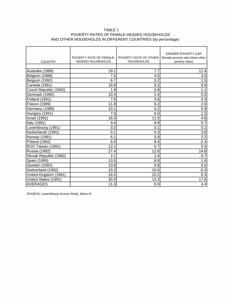
TABLE 1POVERTY RATES OF FEMALE-HEADED HOUSEHOLDS
AND OTHER HOUSEHOLDS IN DIFFERENT COUNTRIES (by percentage)
COUNTRYPOVERTY RATE OF FEMALE-
HEADED HOUSEHOLDSPOVERTY RATE OF OTHER
HOUSEHOLDS
GENDER POVERTY GAP (female poverty rate minus other
poverty rates)
Australia (1989) 19.1 7.7 11.4Belgium (1988) 7.5 4.5 3.0Belgium (1992) 6.7 5.2 1.5Canada (1991) 18.8 9.2 9.6Czech Republic (1992) 1.9 0.8 1.1Denmark (1992) 10.4 5.4 5.0Finland (1991) 7.9 3.6 4.3France (1989) 11.8 9.2 2.6Germany (1989) 10.1 4.2 5.9Hungary (1991) 7.0 6.0 1.0Israel (1992) 16.3 11.5 4.8Italy (1991) 9.6 8.9 0.7Luxembourg (1991) 3.2 3.1 0.1Netherlands (1991) 9.1 5.3 3.8Norway (1991) 6.1 3.9 2.2Poland (1992) 6.0 8.4 -2.4ROC Taiwan (1991) 12.1 6.7 5.4Russia (1992) 27.4 12.6 14.8Slovak Republic (1992) 2.1 1.4 0.7Spain (1990) 10.5 8.9 1.6Sweden (1992) 10.8 5.8 5.0Switzerland (1992) 10.3 10.6 -0.3United Kingdom (1991) 16.5 10.2 6.3United States (1991) 30.9 13.3 17.6AVERAGES 11.3 6.9 4.4
SOURCE: Luxembourg Income Study, Wave III
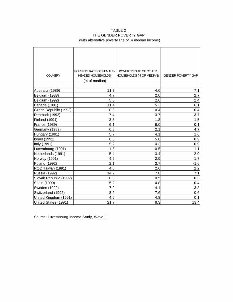
TABLE 3. TABLE 2 THE GENDER POVERTY GAP THE GENDER POVERTY GAP
(with alternative poverty line of .4 median income)
COUNTRYPOVERTY RATE OF FEMALE-
HEADED HOUSEHOLDS POVERTY RATE OF OTHER
HOUSEHOLDS (.4 OF MEDIAN) GENDER POVERTY GAP
(.4 of median)
Australia (1989) 11.7 4.6 7.1Belgium (1988) 4.7 2.0 2.7Belgium (1992) 5.0 2.6 2.4Canada (1991) 11.4 5.3 6.1Czech Republic (1992) 0.8 0.4 0.4Denmark (1992) 7.4 3.7 3.7Finland (1991) 3.3 1.8 1.5France (1989) 6.1 6.0 0.1Germany (1989) 6.8 2.1 4.7Hungary (1991) 5.7 4.1 1.6Israel (1992) 6.5 5.6 0.9Italy (1991) 5.2 4.3 0.9Luxembourg (1991) 1.6 0.5 1.1Netherlands (1991) 5.4 3.4 2.0Norway (1991) 4.6 2.9 1.7Poland (1992) 2.1 3.7 -1.6ROC Taiwan (1991) 4.8 2.6 2.2Russia (1992) 14.9 7.8 7.1Slovak Republic (1992) 0.8 0.5 0.3Spain (1990) 5.2 4.8 0.4Sweden (1992) 7.9 4.1 3.8Switzerland (1992) 8.2 7.6 0.6United Kingdom (1991) 4.9 4.8 0.1United States (1991) 21.7 8.3 13.4
Source: Luxembourg Income Study, Wave III
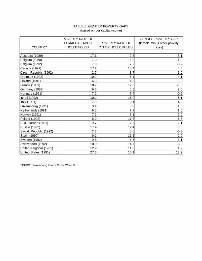
TABLE 3 .GENDER POVERTY GAPS (based on per capita income)
COUNTRY
POVERTY RATE OF FEMALE-HEADED
HOUSEHOLDSPOVERTY RATE OF
OTHER HOUSEHOLDS
GENDER POVERTY GAP (female minus other poverty
rates)
Australia (1989) 17.6 9.5 8.1Belgium (1988) 7.0 6.0 1.0Belgium (1992) 7.0 7.2 -0.2Canada (1991) 17.2 10.4 6.8Czech Republic (1992) 2.7 1.7 1.0Denmark (1992) 10.2 6.1 4.1Finland (1991) 4.3 4.3 0.0France (1989) 10.7 12.0 -1.3Germany (1989) 9.3 6.8 2.5Hungary (1991) 7.2 7.4 -0.2Israel (1992) 10.1 15.2 -5.1Italy (1991) 7.9 12.1 -4.2Luxembourg (1991) 8.4 6.9 1.5Netherlands (1991) 9.5 7.9 1.6Norway (1991) 7.1 5.1 2.0Poland (1992) 5.0 11.6 -6.6ROC Taiwan (1991) 9.7 7.6 2.1Russia (1992) 17.4 12.4 5.0Slovak Republic (1992) 2.7 3.0 -0.3Spain (1990) 9.1 11.1 -2.0Sweden (1992) 9.8 6.7 3.1Switzerland (1992) 10.9 14.7 -3.8United Kingdom (1991) 12.9 11.0 1.9United States (1991) 27.3 15.1 12.2
SOURCE: Luxembourg Income Study, Wave III
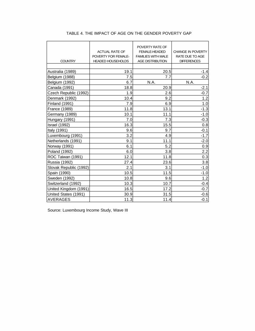
TABLE 4. THE IMPACT OF AGE ON THE GENDER POVERTY GAP
COUNTRY
ACTUAL RATE OF POVERTY FOR FEMALE-HEADED HOUSEHOLDS
POVERTY RATE OF FEMALE-HEADED
FAMILIES WITH MALE AGE DISTRIBUTION
CHANGE IN POVERTY RATE DUE TO AGE
DIFFERENCES
Australia (1989) 19.1 20.5 -1.4Belgium (1988) 7.5 7.7 -0.2Belgium (1992) 6.7 N.A. N.A.Canada (1991) 18.8 20.9 -2.1Czech Republic (1992) 1.9 2.6 -0.7Denmark (1992) 10.4 9.2 1.2Finland (1991) 7.9 6.9 1.0France (1989) 11.8 13.1 -1.3Germany (1989) 10.1 11.1 -1.0Hungary (1991) 7.0 7.3 -0.3Israel (1992) 16.3 15.5 0.8Italy (1991) 9.6 9.7 -0.1Luxembourg (1991) 3.2 4.9 -1.7Netherlands (1991) 9.1 11.1 -2.0Norway (1991) 6.1 5.2 0.9Poland (1992) 6.0 3.8 2.2ROC Taiwan (1991) 12.1 11.8 0.3Russia (1992) 27.4 23.6 3.8Slovak Republic (1992) 2.1 3.1 -1.0Spain (1990) 10.5 11.5 -1.0Sweden (1992) 10.8 9.6 1.2Switzerland (1992) 10.3 10.7 -0.4United Kingdom (1991) 16.5 17.2 -0.7United States (1991) 30.9 31.5 -0.6AVERAGES 11.3 11.4 -0.1
Source: Luxembourg Income Study, Wave III
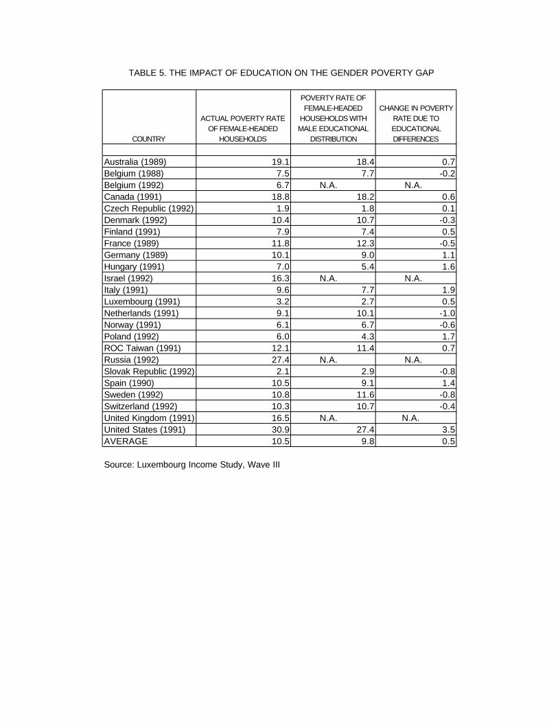
TABLE 5. THE IMPACT OF EDUCATION ON THE GENDER POVERTY GAP
COUNTRY
ACTUAL POVERTY RATE OF FEMALE-HEADED
HOUSEHOLDS
POVERTY RATE OF FEMALE-HEADED
HOUSEHOLDS WITH MALE EDUCATIONAL
DISTRIBUTION
CHANGE IN POVERTY RATE DUE TO EDUCATIONAL DIFFERENCES
Australia (1989) 19.1 18.4 0.7Belgium (1988) 7.5 7.7 -0.2Belgium (1992) 6.7 N.A. N.A.Canada (1991) 18.8 18.2 0.6Czech Republic (1992) 1.9 1.8 0.1Denmark (1992) 10.4 10.7 -0.3Finland (1991) 7.9 7.4 0.5France (1989) 11.8 12.3 -0.5Germany (1989) 10.1 9.0 1.1Hungary (1991) 7.0 5.4 1.6Israel (1992) 16.3 N.A. N.A.Italy (1991) 9.6 7.7 1.9Luxembourg (1991) 3.2 2.7 0.5Netherlands (1991) 9.1 10.1 -1.0Norway (1991) 6.1 6.7 -0.6Poland (1992) 6.0 4.3 1.7ROC Taiwan (1991) 12.1 11.4 0.7Russia (1992) 27.4 N.A. N.A.Slovak Republic (1992) 2.1 2.9 -0.8Spain (1990) 10.5 9.1 1.4Sweden (1992) 10.8 11.6 -0.8Switzerland (1992) 10.3 10.7 -0.4United Kingdom (1991) 16.5 N.A. N.A.United States (1991) 30.9 27.4 3.5AVERAGE 10.5 9.8 0.5
Source: Luxembourg Income Study, Wave III
Recommended