Chapman UniversityChapman University Digital Commons
ESI Working Papers Economic Science Institute
2015
Status and the Demand for Visible Goods:Experimental Evidence on ConspicuousConsumptionDavid ClingingsmithCase Western Reserve University, Cleveland, Ohio
Roman M. SheremetaChapman University
Follow this and additional works at: http://digitalcommons.chapman.edu/esi_working_papers
Part of the Econometrics Commons, Economic Theory Commons, and the Other EconomicsCommons
This Article is brought to you for free and open access by the Economic Science Institute at Chapman University Digital Commons. It has beenaccepted for inclusion in ESI Working Papers by an authorized administrator of Chapman University Digital Commons. For more information, pleasecontact [email protected].
Recommended CitationClingingsmith, D. and Sheremeta, R.M. (2015). Status and the demand for visible goods: Experimental evidence on conspicuousconsumption. ESI Working Paper 15-27. Retrieved from http://digitalcommons.chapman.edu/esi_working_papers/176

Status and the Demand for Visible Goods: Experimental Evidence onConspicuous Consumption
CommentsWorking Paper 15-27
This article is available at Chapman University Digital Commons: http://digitalcommons.chapman.edu/esi_working_papers/176
1
Status and the Demand for Visible Goods:
Experimental Evidence on Conspicuous Consumption
David Clingingsmith a,*
Roman M. Sheremeta a,b
a Weatherhead School of Management, Case Western Reserve University
11119 Bellflower Road, Cleveland, OH 44106, U.S.A. b Economic Science Institute, Chapman University
One University Drive, Orange, CA 92866, U.S.A.
December 4, 2015
Abstract
Some economists argue that consumption of publicly visible goods is driven by
social status. Making a causal inference about this claim is difficult with
observational data. We conduct an experiment in which we vary both whether a
purchase of a physical product is publicly visible or kept private and whether the
income used for purchase is linked to social status or randomly assigned. Making
consumption choices visible leads to a large increase in demand when income is
linked to status, but not otherwise. We investigate the characteristics that mediate
this effect and estimate its impact on welfare.
JEL Classifications: C91, D03
Keywords: status, conspicuous consumption, experiment
* Corresponding author: David Clingingsmith, E-mail: [email protected] or [email protected]
We thank Yan Chen, Ori Heffetz, David Huffman, John List, Tanya Rosenblat, Klaus Schmidt, Justin Sydnor, Lise
Vesterlund, Alistair Wilson, Bart Wilson and seminar participants at Case Western Reserve University, Chapman
University, Kent State University, the University of Michigan, the University of Pittsburgh as well as participants at
the North American Economic Science Association Meetings in Dallas for helpful comments. We also thank the
Weatherhead School of Management for generous funding of this project and Sarah Mattson for excellent research
assistance. The usual disclaimers apply.
2
1. Introduction
Social status refers to the hierarchical position an individual occupies in society. Social
status is related to an individual’s attributes, such as intelligence, creativity, beauty, affiliation, or
family of origin, either through the returns such attributes earn in economic activity or the esteem
in which they are held by society, or both.1
Veblen argued that social status has a profound influence on a person’s consumption
decisions. His book The Theory of the Leisure Class contends that status concerns affect the
consumption choices of anyone whose income places them above the level of subsistence (2009
[1899]). Social conventions specify a minimum standard of clothing, food, and living conditions
that are acceptable for each status level. Since social status and income are positively correlated,
the acceptable standard of consumption for those of higher status includes more and better goods
than for those of lower status. According to Veblen, an important function of consumption is to
signal high status to others. Consumption choices can only do this to the extent they are both visible
to others and associated with high status. Part of the motivation for wearing a fine suit or driving
a luxury car, both of which are visible to others, is to convey the message to others that one has
high status.
Consumer goods vary in the degree to which the act of consuming them is visible to the
public, and thus in their suitability for serving as public markers of status. Many people see us
when we are in our cars, when we wear our work clothes, or when we eat at a restaurant. Far fewer
1 See a more detailed discussion at http://www.britannica.com/topic/social-status.
3
see our sleepwear, what we have for breakfast at home, or the brand of toilet paper we buy.2 Veblen
termed status signaling via the acquisition and display of visible goods conspicuous consumption.3
A number of studies have presented evidence about the relationship between status and the
consumption of visible goods (Ravina, 2007; Grinblatt et. al. 2008; Charles et. al., 2009; Heffetz,
2011; Kuhn et al., 2011). However, there are several difficulties in identifying conspicuous
consumption as a motivation for consuming visible goods. First, visibility is only one of many
properties possessed by any given good that contribute to the observed demand for it. It is difficult
to disentangle demand for visibility from demand for these other properties. While we may
conjecture that a person buys a Mercedes rather than a Toyota to signal high social status, a
Mercedes is a superior car in many ways besides the signal it sends about status. A second, subtly
related problem is the link between income and social status. Income has effects on consumption
that are independent of any status motivation. Observed correlations between status and
consumption could be pure income effects. Income also tends to be correlated with various
characteristics that confer social status through popular esteem, such as intelligence, education
level, family background, profession, and political clout. Lastly, it is difficult to disentangle
conspicuous consumption from social learning as factors that drive individuals with similar social
status to make similar consumption decisions (Grinblatt et al., 2008).
We tackle the challenge of identifying conspicuous consumption by conducting a
controlled experiment. In our experiment, individuals have an opportunity to purchase a desirable
2 With the rise of social networks and associated technologies such as the smartphone, many formerly private choices,
such as food consumed at home or the decoration of private spaces, have become increasingly visible to the public.
Everyday millions of people post descriptions and images from their private lives on social networks such as Facebook
and Instagram that feature the goods they consume. 3 Several attempts have been made over the years to develop Veblen’s ideas within a more formal microeconomic
framework. Following Leibenstein (1950), some authors have mistakenly attempted to capture Veblen’s argument
with the notion that price is directly a part of utility. Veblen’s analysis implies instead that the determinants of utility
are consumption and social status in the eyes of others. Those goods which signal social status must be visible, but
signaling may occur both through quantity and quality/price (Bagwell and Bernheim, 1996).
4
consumer good: gourmet chocolate truffles. We independently vary both the visibility of
consumption choices to others and whether the income available for consumption is linked to
social status.4 After accruing income, each participant indicates their desired quantity of chocolate
truffles for each of several potential prices. A common price at which sales are actually made is
randomly selected from the potential prices at the end of the experiment.
We manipulate this process in two ways, using a two-by-two design. In the first
manipulation, income is either assigned randomly or based on a participant’s rank. A participant’s
rank is determined how well they do relative to the eleven other participants in their experimental
session on a thirty-minute cognitive test. Our participants are students at Case Western Reserve
University (CWRU). As at many elite universities, cognitive ability confers social status at
CWRU.5 When income is assigned by rank it is directly correlated with status, but when it is
assigned randomly it is unrelated to status. In the second manipulation, communication about the
quantity of truffles purchased is either private, so that only the participant and experimenter know,
or public, so that all participants in the experimental session can see how much each purchased.
Participants know how their choices will be communicated before making them. We refer to the
four treatments as rank-private, rank-public, random-private, and random-public.
Our design allows us to isolate the effect of visibility on demand since all other properties
of the chocolate truffles are identical across the public and private treatments. We can also isolate
the effect of the linkage between income and status. We can rule out social learning as a driver of
4 Our study is related to a large literature on status signaling as a motivation for charitable giving and behavior in
social dilemmas (Andreoni and Petrie, 2004; Soetevent, 2005; Andreoni et al., 2009; Ariely et al., 2009; Bracha and
Vesterlund, 2013; Karlan and McConnell, 2014; Samek and Sheremeta, 2014, 2015). However, our use of a physical
product as a status signal eliminates confounds present in previous studies. Buying chocolate provides only private
benefit to the person who purchased it, while charitable giving and social dilemmas provide benefits to others as well.
Our study therefore does not involve the confounding factors of generosity and altruism present in these other studies. 5 While cognitive ability is a source of social status in general, it is particularly important in the social world of
university students.
5
consumption decisions within the experiment because our participants do not interact and have no
information about the choices of others when they make their decisions.
Veblen’s theory of conspicuous consumption predicts that demand will be higher in rank-
public than rank-private because when status is linked to income, visibility leads people to
consume more to signal status. To the extent that by assigning income randomly we completely
sever the link to status, Veblen’s theory also predicts that demand will be the same in random-
public and random-private.
Consistent with these predictions, we find that making consumption choices publicly
visible leads to a large increase in demand when income is linked to status, but not when income
is assigned randomly. In other words, we find that the necessary conditions for conspicuous
consumption are 1) for income to be correlated with status and 2) for consumption choices to be
publicly visible to others. The effect is quite large: mean quantity demanded is 1.94 truffles in
rank-private and 4.98 truffles in rank-public, an increase of 257%. When income is unrelated to
status, visibility does not induce conspicuous consumption: mean quantity demanded is 1.74 in
random-private and 1.75 in random-public. Although our data provide support for a hypothesis
that status is a significant factor motivating consumption of visible goods, the relationship between
status level and conspicuous consumption is non-monotonic.6 Therefore, a person’s income (and
thus the social status) cannot be easily inferred from their actual chocolate choice in rank-public.
We find that gender and cognitive reflection are important mediators of conspicuous
consumption. Men engaged in conspicuous consumption much more than women. Quantity
6 We find that participants of moderately high and moderately low status engage in conspicuous consumption more
than participants of middle status. Such non-monotonicities are possible in signaling games when players counter-
signal (Spence, 1973; Feltovich et al., 2002). This equilibrium may reflect signaling being relatively cheap: The
lowest-rank person earned $5.25 and the average truffle consumption was 2 in rank-private, so even the lowest-rank
person could inexpensively engage in signaling competition.
6
demanded by men is 477% higher in rank-public than rank-private. Individuals who scored high
on a measure of cognitive reflection (Frederick, 2005), which is the propensity to engage in
conscious deliberation when a situation requires it, also engage more in conspicuous consumption.
We find no impact of risk aversion or competitive social preferences on conspicuous consumption.
Publicly visible choice causes participants to buy chocolate truffles at higher prices than
they would have otherwise. By comparing the demand curves in rank-private and rank-public, we
can estimate both the rank-private consumer surplus and the average welfare loss from making
consumption public. We find that the average welfare loss is as large as the consumer surplus when
the price of chocolate is $0.40, which is approximately the retail price. The negative effect of
conspicuous consumption on welfare loss comes primarily from men, who account for most of the
conspicuous consumption. For women, the loss is much smaller and insignificant.
The non-monotonic relationship between consumption and income means that public
consumption does not convey a credible signal about status, which means that the welfare loss
from conspicuous consumption is not compensated by signaling value of such consumption. To
investigate whether participants derive utility from conspicuous consumption unrelated to
signaling, we asked them to rate their mood at the end of the experiment. For men, we find no
difference in self-reported mood between rank-public and rank-private. To the extent that our
simple mood measure captures the non-consumption externalities of status signaling, it provides
suggestive evidence that the net welfare effect of conspicuous consumption is negative for men.
Women’s moods are low in rank-private, so the net welfare effect of conspicuous consumption
for them is likely positive. However, it is possible that our measure does not fully capture the non-
consumption externalities of status signaling. We discuss some possibilities in the conclusion.
7
We describe the experimental design and procedures in Section 2. Our main results are
presented in Section 3, along with analyses of how conspicuous consumption is related to the level
of status, the characteristics of those who engage in conspicuous consumption, and the welfare
effects of conspicuous consumption. We discuss connections to the literature and implications of
our results in Section 4.
2. Experimental Design and Procedures
The experiment was conducted at Case Western Reserve University. We recruited
participants from an email pool of undergraduate and graduate students. There were 12 sessions
with 12 participants each, for a total of 144 participants. Participants were seated in an ordinary
classroom. The experiment consisted of several parts and participants received instructions
(available in Appendix A) at the beginning of each part.
In all sessions, participants completed a 30-minute cognitive test consisting of 20 multiple-
choice questions. The questions were drawn from a Graduate Record Examination (GRE) test
preparation book (Seltzer, 2009). There were 10 mathematical and 10 verbal questions. All were
of moderate to high difficulty. Participants worked using pencil and paper and recorded their
responses on bubble sheets. The sheets were scanned and scored after 30 minutes had elapsed.
Each participant received one point for each correct response and lost one point for each incorrect
answer. Unanswered questions carried no penalty. Participants were ranked according to the
resulting score, and received a sheet indicating their score and rank among their fellow participants.
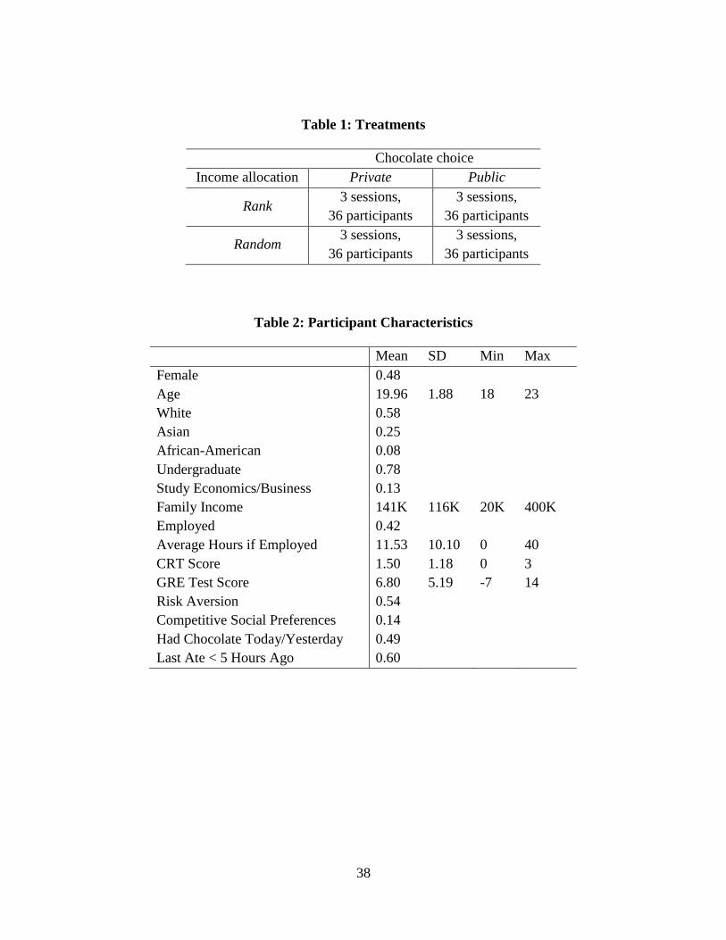
We employed the two-by-two design shown in Table 1. The first treatment manipulation
varied the manner in which participants received income. There were 12 income levels between
$5 and $13.25. In the rank treatments, income was allocated based on each participant’s rank on
8
the test. The participant who ranked first on the test got $13.25, while the participant who ranked
last got $5. Participants were given a table showing how rank translated into income with their
own rank and income circled. In the random treatments, income was allocated using a random
draw without replacement. Participants privately drew a card from bag containing cards numbered
1 through 12. Each participant had a table showing how the random numbers translated into
income, from $5 for number 12 to $13.25 for number 1. As a result of this procedure, income and
performance on the test are positively correlated in the rank treatments and uncorrelated in the
random treatments.
Participants were then given an opportunity to spend some of their income on gourmet
chocolate truffles. We chose gourmet chocolate truffles because 1) they are a rival and excludable
consumption good; 2) they are desirable to participants; 3) they are packaged as small, discrete
pieces; and 4) they are of high quality. We wanted a rival and excludable good rather than a public
good, such as a donation to charity, because the benefit of consuming it is purely private. The
motivations underlying demand for rival and excludable goods are less complex, which makes
interpretation of behavior clearer.
Participants completed a table that listed nine potential truffle prices between $0.20 and
$0.60. We asked each participant to indicate how many truffles they would like to purchase at each
of nine potential prices and explained that the roll of a die would later determine the actual price.
They could indicate any quantity between zero and a number exhausting their total income and
would then purchase the indicated quantity corresponding to the actual price. Participants were
told that the remaining cash would be paid to them at the end of the session. Calculators were
provided for this portion.
9
The second treatment manipulation varied how the participants would communicate the
quantity of chocolate they purchased. Before participants completed the table of chocolate choices,
we told them how they would receive their selection once the actual price was determined. In the
private treatments, we explained that we would collect their selection tables and package the
chocolate at the side of the classroom in brown paper bags labeled with their subject numbers. This
would keep everyone’s selections private. Bags would be distributed as participants came up to
get their payments at the end of the experiment. Each participant would get a bag regardless of
whether they purchased any chocolate. In the public treatments, participants were told that after
the actual price was determined, each participant would come up to the whiteboard and write the
quantity of chocolate they selected and the total cost along with their first name and subject
number. We told them that this would speed up our packaging of the chocolate and computation
of payments, which was true.
We collected several other types of data to help us understand what individual
characteristics might mediate the effects of our treatments. Before the GRE test, we measured
cognitive reflection. After participants completed their chocolate choice tables but before the
actual price was determined, we collected measures of risk aversion, social preferences, and
demographic characteristics. The risk aversion and social preferences measures were incentivized.
The three-question cognitive reflection test (CRT) was participants’ first task in the session
(Frederick, 2005). The CRT questions are simple math problems designed to have an intuitively
appealing solution that is incorrect. The test measures an individual’s ability to resist their intuition
and arrive at the correct solution. For example, the first question is “A bat and a ball cost $1.10 in
total. The bat costs $1.00 more than the ball. How much does the ball cost?” The appealing but
incorrect answer is $0.10. The correct answer is $0.05.
10
Participants made a series of 20 binary choices to measure risk aversion (similar to Holt
and Laury, 2002). The choices involved a risk-free amount varying from $0.50 to $10.00 and a
lottery offering a 50% chance to get $10 and a 50% chance to get nothing (see Appendix A). One
of the 20 choices was randomly selected to be paid out at the end of the experiment. We measure
risk aversion using a dummy that identifies whether a participant was more risk averse than the
median.
Next, participants made 12 binary choices to measure social preferences (similar to
Charness and Rabin, 2002). The choices involved additional income for themselves and another
participant with whom they were anonymously paired. Each choice offered the option of $3 to
both self and other or an unequal amount with total value between $3.50 and $8.50 (see Appendix
A). One of the 12 choices was randomly selected to be paid out at the end of the experiment, and
one of the paired participants was randomly selected to be the decision maker, while the other was
selected as a receiver. We use these choices to distinguish participants who always maximize social
welfare from those with competitive preferences. We define a measure of competitive social
preferences as the share of choices in which a participant sacrificed social welfare to increase the
amount by which their payment would be greater than the receiver.
Finally, at the end of the experiment, random draws were conducted to determine payouts
for the risk aversion and social preferences choices as well as the price of chocolate. As the
chocolate was being packaged at the end of the experiment, participants completed a demographic
survey. On average participants earned $15.18 and the experiment lasted for about 70 minutes.
11
3. Results
In this section we present the main results. We start by describing participant characteristics
and our main findings. We then examine how conspicuous consumption is related to status level
and what types of participants are most likely to engage in conspicuous consumption. Finally, we
analyze the welfare effects of conspicuous consumption.
3.1 Participant Characteristics
Table 2 shows the characteristics of our 144 participants. Over three-quarters of our
participants are undergraduate students. They come from a wide range of majors and departments.
Only 13% of participants study economics, finance, or another business-related field. On average,
participants are 20 years old. Gender composition is balanced, with 48% female and 52% male
students. Whites make up 58%, Asians 25%, and African-Americans 8%. The average income in
their family of origin is $141,000. About 42% work in addition to studying, and of those who do,
the average work week is 11.5 hours. Overall, our participant pull is representative of the student
body of Case Western Reserve University.
3.2. Main Findings
Our main question of interest is whether participants engage in conspicuous consumption.
If there is no conspicuous consumption, we should observe no difference in demand for chocolate
across our treatments. If there is conspicuous consumption when income is linked to social status,
we should observe greater demand in rank-public than rank-private. If conspicuous consumption
is about signaling one’s income level itself, we should observe greater demand in random-public
than random-private.
12
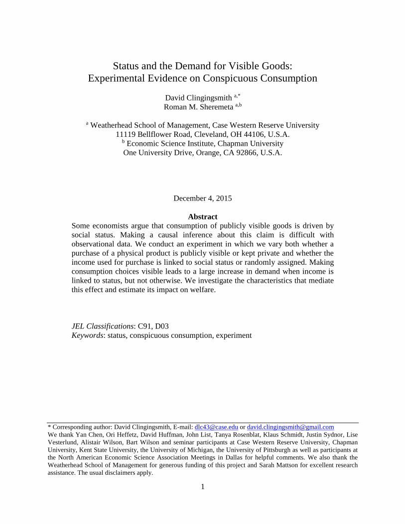
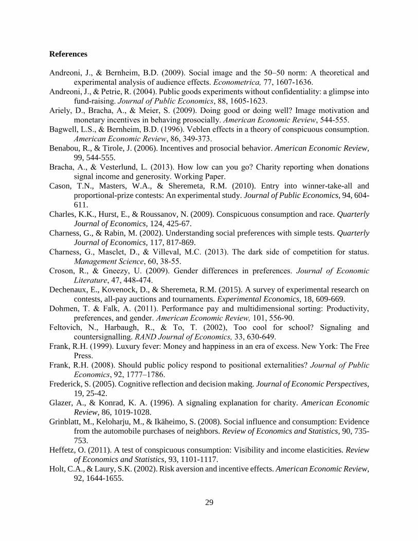
Figure 1 shows aggregate chocolate demand curves for each of the four treatments. The
markers show the total quantity demanded at each potential price for the 36 participants in each
treatment. Across all treatments, as standard microeconomic theory predicts, the quantity
demanded falls as price increases. Demand for chocolate in the rank-public treatment is much
higher than the other three treatments. The demand shift is so large that this curve has limited
overlap with the others despite price varying by a factor of three. The curves tell us that making
choices publicly visible increases demand when income is related to status but not when it is
assigned randomly.
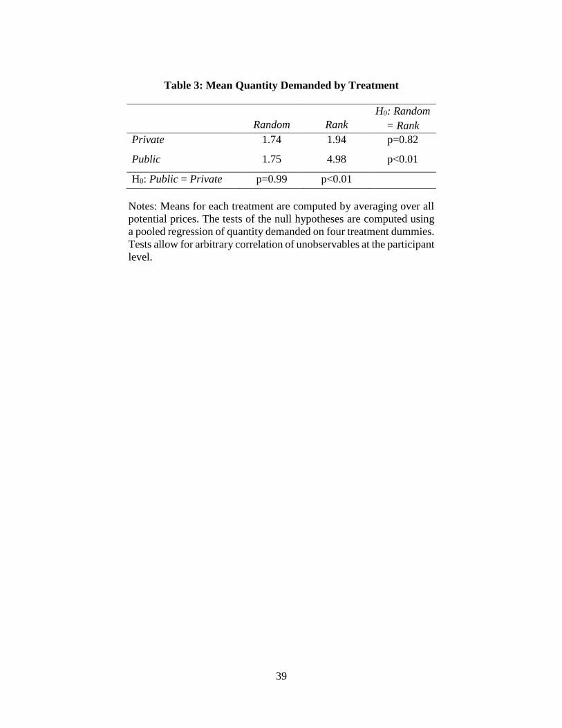
We show the average quantity demanded over all potential prices for the four treatments
in Table 3. Mean quantity demanded is 1.94 in rank-private and 4.98 in rank-public, a large and
statistically significant difference of 257%. The total income available to spend on chocolate is the
same in rank-public and rank-private, and its distribution in terms of test performance is also the
same. This allows us to interpret the increased consumption as a causal effect of making
consumption visible. By contrast, when income is assigned randomly rather than by test rank,
mean quantity demanded is 1.74 in random-private and 1.75 in random-public. Again, the total
income available to spend on chocolate is the same in random-public and random-private, and its
distribution in terms of test performance is also the same. This tells us that visibility alone is not
enough to induce an increase in consumption. Income must be correlated with status, here
performance on the test, for public visibility to induce conspicuous consumption. In other words,
the necessary conditions for conspicuous consumption are 1) income must be correlated with status
and 2) consumption choices must be publicly visible to others.
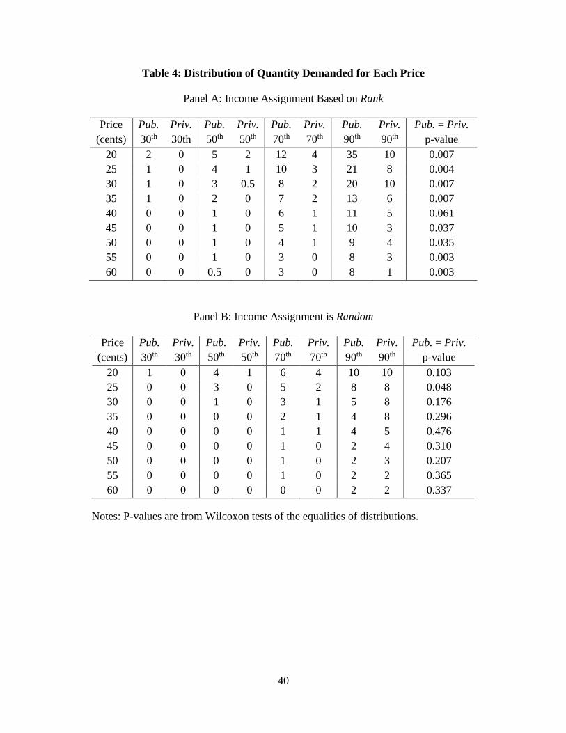
We explore how quantiles of demand vary by treatment for different prices in Table 4.
Panel A compares rank-private and rank-public. All quantiles of demand are higher in the rank-
13
public treatment for every price level. A Wilcoxon rank-sum test at each price level shows the
differences in distributions to be statistically significant. All but one of the p-values are less than
0.05 and most are less than 0.01. Panel B compares random-private and random-public. The
Wilcoxon test shows no statistically significant difference in the distributions at any price other
than $0.25. Overall, the detailed analysis shows that differences found for means from Table 3 are
reflected at all prices and parts of demand curves.
Treatments were randomly assigned to experimental sessions, so the expectation is for
participants in each session to be the same on average in terms of their characteristics. It is
nevertheless possible that participants in different sessions differ in ways important for demand.
To check the robustness of our results, we conduct a regression analysis in which we examine
whether controlling for observable characteristics affects our results.
Let 𝑞𝑖𝑝 be the chocolate demanded by individual 𝑖 when the price is 𝑝, 𝑋𝑖 be a vector of
characteristics for 𝑖, 𝑃𝑢𝑏𝑙𝑖𝑐𝑖 indicate whether consumption choice of 𝑖 is public, and 𝑅𝑎𝑛𝑘𝑖
indicate whether 𝑖’s income was assigned by test rank. Our specification is then
𝑞𝑖𝑝 = 𝛼 + 𝛽𝑃𝑃𝑢𝑏𝑙𝑖𝑐𝑖 + 𝛽𝑅𝑅𝑎𝑛𝑘𝑖 + 𝛽𝑃𝑅(𝑃𝑢𝑏𝑙𝑖𝑐𝑖 × 𝑅𝑎𝑛𝑘𝑖) + 𝑋𝑖′𝜃 + 𝜀𝑖𝑝. (1)
When estimating this regression, we compute standard errors allowing for arbitrary correlation of
𝜀𝑖𝑝 within each individual. Our control vector includes the characteristics we elicited from our
participants as shown in Table 2.
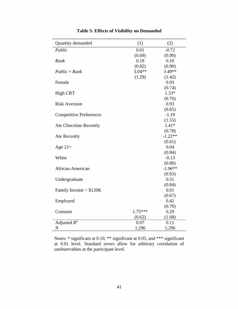
Table 5 reports the results of estimating equation (1) using OLS. Column 1 shows estimates
without any controls. The constant shows average quantity demanded in random-private. Average
quantity demanded in other treatments replicating the means from Table 2 may be obtained by
adding the appropriate coefficients from the set 𝑃𝑢𝑏𝑙𝑖𝑐, 𝑅𝑎𝑛𝑘, and 𝑃𝑢𝑏𝑙𝑖𝑐 × 𝑅𝑎𝑛𝑘. Notably, the
differences in average quantity demanded computed from the regression are 3.04 (p<0.01) between
14
rank-public and rank-private and 0.01 (p=0.99) between random-public and random-private.
Column 2 adds in controls for participant characteristics. Demand is higher for those who have
consumed chocolate in the recent past and lower for those who have eaten in the past five hours,
which makes intuitive sense. Demand is also lower for African-Americans. However, addition of
the controls does not measurably affect the differences between treatments. Conditional on
controls, the differences in average quantity demanded are 3.39 (p<0.01) between rank-public and
rank-private and -0.72 (p=0.26) between random-public and random-private.
Result 1: Making consumption choices visible strongly increases demand when income is
linked to status, but not when income is assigned randomly.
3.3. Levels of Status and Conspicuous Consumption
Chocolate demand is higher when consumption is public for participants whose income
was assigned according to rank, suggesting that participants engage in conspicuous consumption
by buying chocolate to signal their status. In this section, we examine whether conspicuous
consumption varies by status level. If high consumption of visible goods serves as a signal of high
status, we might expect the relationship between a person’s level of status and the degree to which
they engaged in conspicuous consumption to be positive. However, if individuals signal
strategically, then it is also possible to obtain non-monotonic relationship between status and
conspicuous consumption, especially if some participants choose to countersignal their status
(Spence, 1973; Feltovich et al., 2002).
In our experiment, status is conferred by one’s rank on the cognitive test. When income is
assigned by rank, status and income are directly correlated. Previously, we established that
conspicuous consumption takes place when income is assigned by rank. To uncover how
15
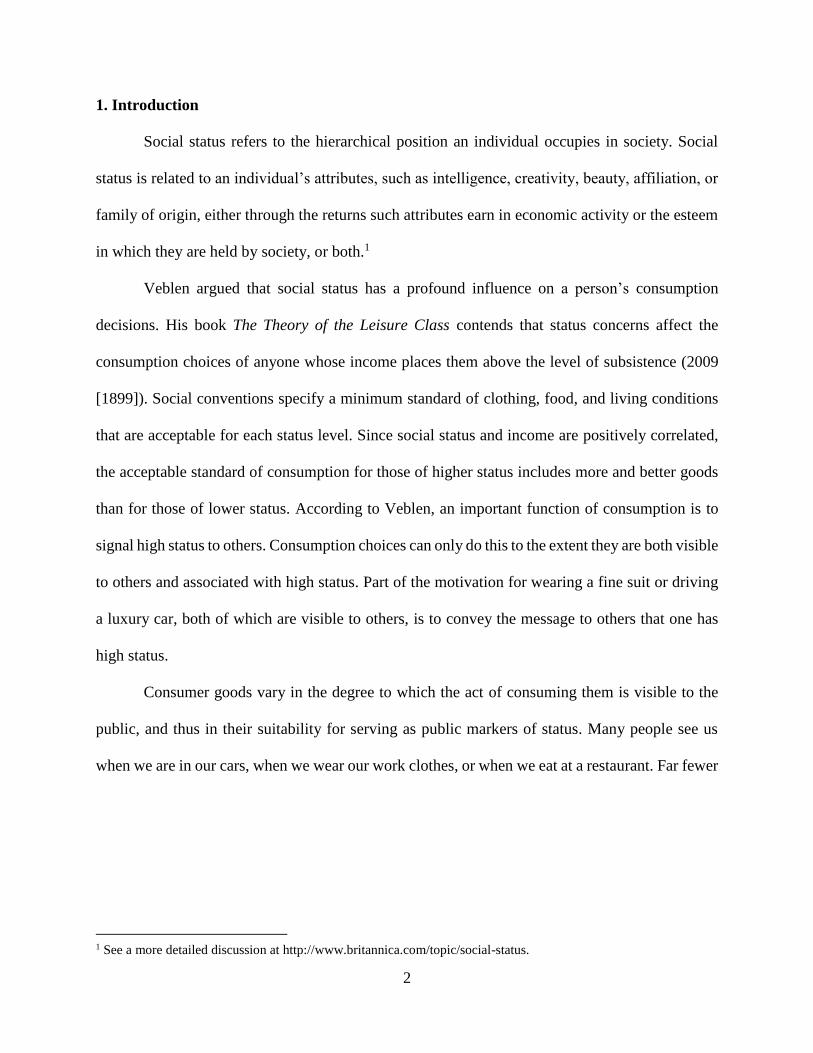
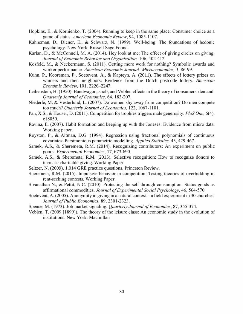
conspicuous consumption is related to rank, we plot Engel curves for chocolate demand. The Engel
curve shows how the share of income spent on chocolate varies with income. Figure 2 displays
Engel curves for all four treatments of our experiment. On the vertical axis, participants are binned
by six income levels. On the horizontal axis, the share of income spent on chocolate is averaged
across all nine potential prices for each participant. All four curves appear non-monotonic, though
we must be cautious in interpreting the shapes as there are only six observations behind each data
point. As with total demand, the rank-private Engel curve stands out as distinct from the other
treatments.
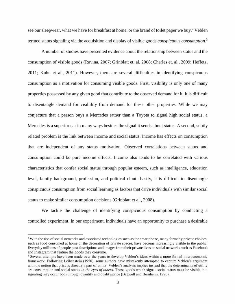
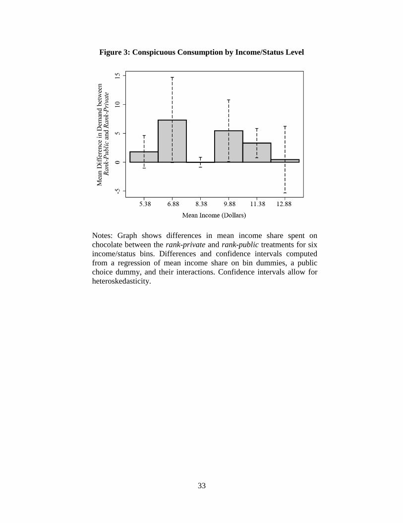
We focus on the difference between the rank-private and rank-public curves in Figure 3.
The graph shows the mean effect of visibility on demand for six income/rank levels computed
using regression. Confidence intervals for each difference are shown using dotted lines.
Conspicuous consumption is clearly non-monotonic in status. Participants of moderately low and
moderately high status are most affected. Those in the middle are less affected.
Result 2: Status level has a non-monotonic impact on conspicuous consumption, with
participants of moderately high and moderately low status engaging in conspicuous consumption
more than participants of middle status.
3.4. Who Engaged in Conspicuous Consumption?
In this section we explore to what extent conspicuous consumption is mediated by
individual characteristics such as gender, risk aversion, competitive social preferences, and
cognitive reflection. We collected information about these characteristics because we suspected
that there could be similarities between conspicuous consumption and competitive behavior. In
particular, in signaling through consumption it is important to consume more than others. A
16
number of studies have documented that competitive behavior is linked to gender (Niederle and
Vesterlund, 2007), risk preferences (Cason et al., 2010), and competitive social preferences
(Dohmen and Falk, 2011).7 We also suspected that cognitive reflection (Frederick, 2005) could be
important because our treatment manipulations require participants to be sensitive to a social
setting they are in.
We investigate these mediating factors through a regression of the quantity of chocolate
demanded at the price-individual level on a dummy variable 𝑃𝑢𝑏𝑙𝑖𝑐𝑖 for the public treatment, a
dummy variable 𝑀𝑖 that categorizes the mediating factor, the interaction 𝑃𝑢𝑏𝑙𝑖𝑐𝑖 × 𝑀𝑖, and a
vector of additional controls 𝑋𝑖.
𝑞𝑖𝑝 = 𝛼 + 𝛽𝑃𝑃𝑢𝑏𝑙𝑖𝑐𝑖 + 𝛽𝑃𝑀(𝑃𝑢𝑏𝑙𝑖𝑐𝑖 × 𝑀𝑖) + 𝛾𝑀𝑖 + 𝑋𝑖′𝜃 + 𝜀𝑖𝑝. (2)
The coefficient 𝛽𝑃 measures the effect of making choice public for those who have a zero value
for the mediating factor dummy while 𝛽𝑃𝑀 measures the differential effect of public choice on
those who have a value of one for the dummy. We control flexibly for test rank by including a
dummy variable for each of the 12 test ranks in the control vector 𝑋𝑖.
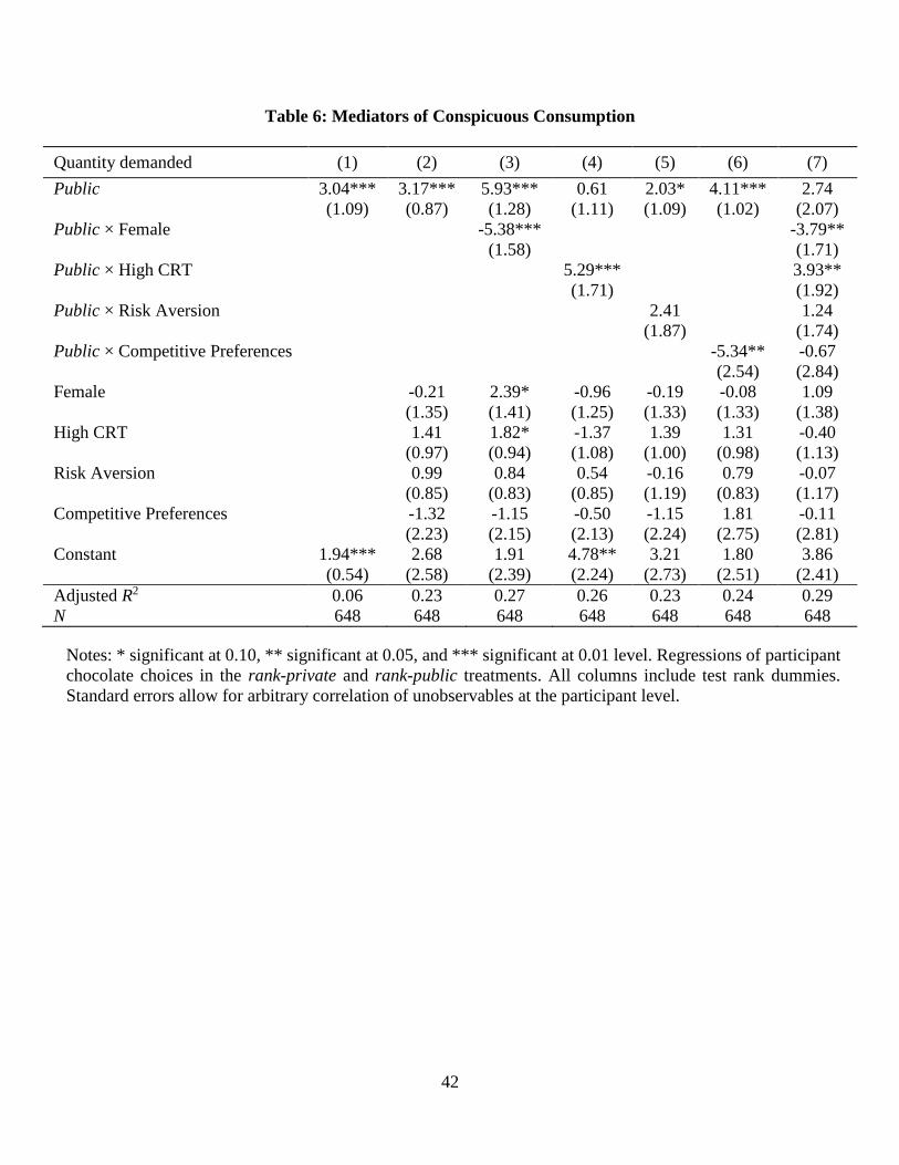
Table 6 reports the estimation results of specification (2). The unconditional effect on
quantity demanded of making consumption public is 3.04 (column 1). The mediators have no
statistically significant effects of their own on quantity demanded when added as controls, and the
coefficients are much smaller than the effect of public choice, which remains unchanged (column
2). Adding the interaction of public with female gender shows that the effect of public choice
comes entirely from men. The effect for men is 5.93 (p<0.01), while for women it is only 0.55 and
is not statistically significantly different from zero (column 3). Similarly, visibility seems to
primarily affect those individuals who have high CRT scores. The effect for high CRT individuals
7 For a review of this literature see Dechenaux et al. (2015).
17
is 5.29 (p<0.01), while it is only 0.61 and not significantly different from zero for low CRT scorers
(column 4). Recall that these regressions control for cognitive test rank. CRT scores are,
unsurprisingly, correlated with cognitive test scores (Spearman’s 𝜌=0.55). The effect measured
here is therefore for that aspect of CRT not correlated with the cognitive test (e.g., impulsivity of
behavior).8 Participants with higher risk aversion are more affected by visibility, though the effect
is not statistically significant (column 5). Having above-median competitive social preferences
reduce the impact of public consumption (column 6). When we include all mediators in the
regression, gender and cognitive reflection remain important mediators (column 7). The
magnitudes are not much changed from the separate regressions. Interestingly, competitive social
preferences are correlated with gender and CRT, which helps explain why the interaction of
competitive social preferences with public consumption is attenuated in the full regression.
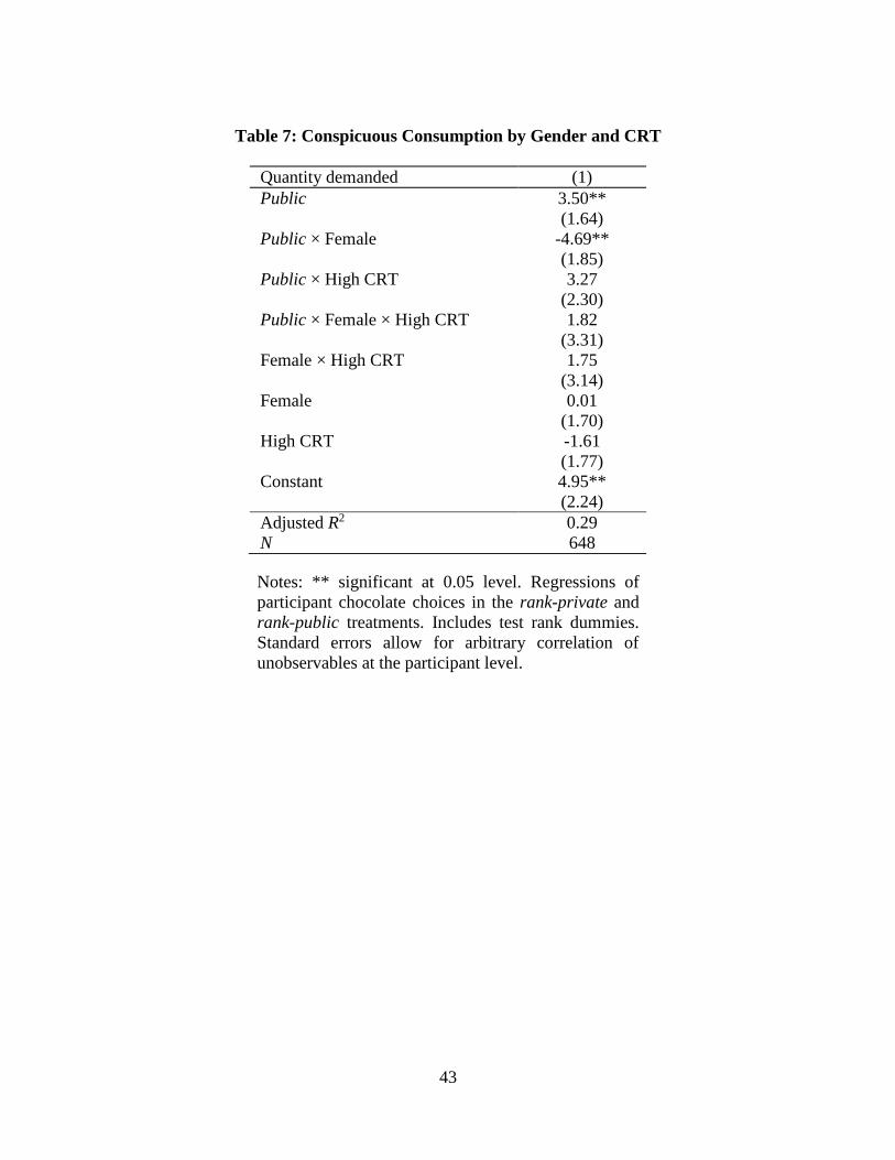
Given that gender and cognitive reflection are the most robust mediators, we now compute
the effect of conspicuous consumption on the four CRT-gender groups. We use the following
regression:
𝑞𝑖𝑝 = 𝛼 + 𝛽1𝑃𝑢𝑏𝑙𝑖𝑐𝑖 + 𝛽2(𝑃𝑢𝑏𝑙𝑖𝑐𝑖 × 𝐹𝑒𝑚𝑎𝑙𝑒𝑖) + 𝛽3(𝑃𝑢𝑏𝑙𝑖𝑐𝑖 × 𝐶𝑅𝑇𝑖) + 𝛽4(𝑃𝑢𝑏𝑙𝑖𝑐𝑖 ×
𝐹𝑒𝑚𝑎𝑙𝑒𝑖 × 𝐶𝑅𝑇𝑖) + 𝛾1𝐹𝑒𝑚𝑎𝑙𝑒𝑖 + 𝛾2𝐶𝑅𝑇𝑖 + 𝛾3(𝐹𝑒𝑚𝑎𝑙𝑒𝑖 × 𝐶𝑅𝑇𝑖) + 𝑋𝑖′𝜃 + 𝜀𝑖𝑝. (3)
In the regression 𝐹𝑒𝑚𝑎𝑙𝑒𝑖 is a dummy variable for female gender and 𝐶𝑅𝑇𝑖 is a dummy for high
CRT.
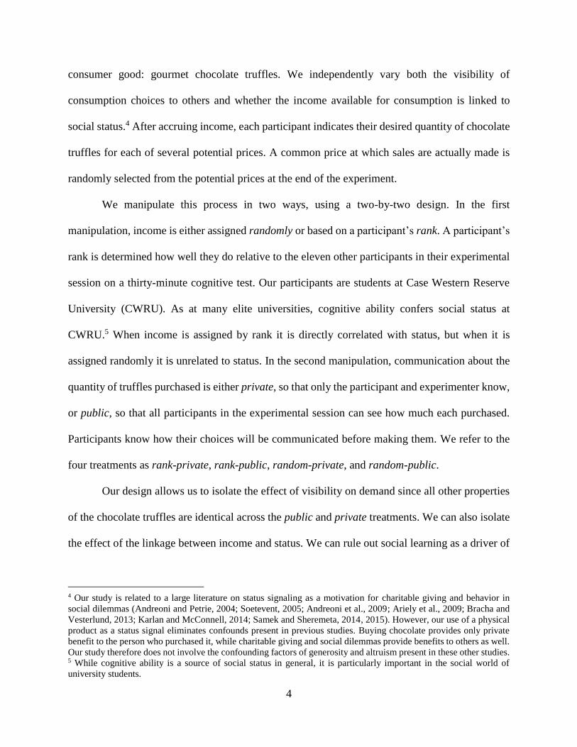
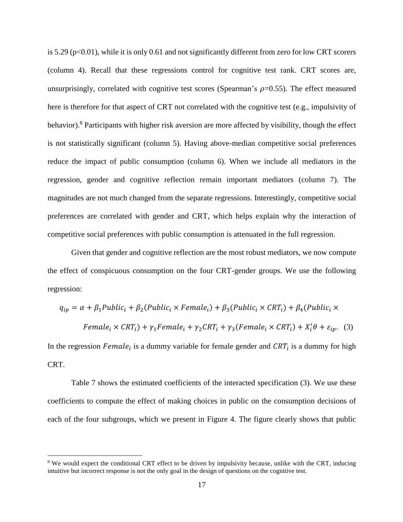
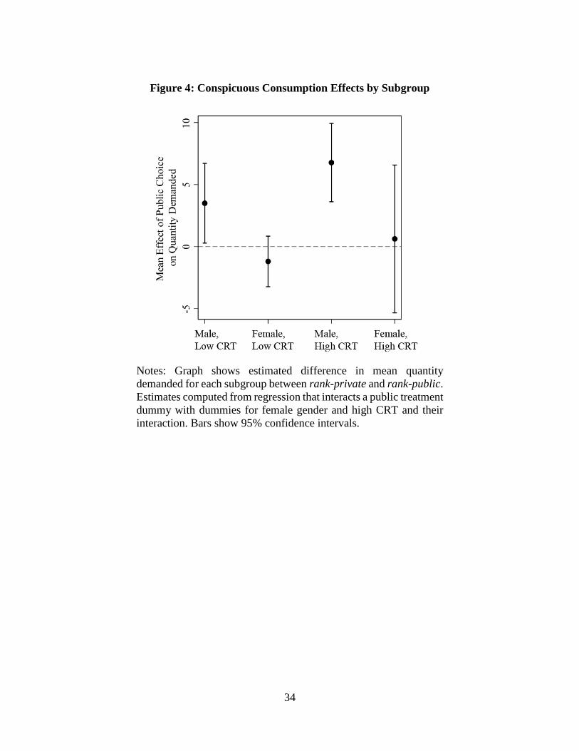
Table 7 shows the estimated coefficients of the interacted specification (3). We use these
coefficients to compute the effect of making choices in public on the consumption decisions of
each of the four subgroups, which we present in Figure 4. The figure clearly shows that public
8 We would expect the conditional CRT effect to be driven by impulsivity because, unlike with the CRT, inducing
intuitive but incorrect response is not the only goal in the design of questions on the cognitive test.
18
consumption has an effect on all male participants, though the effect is greater on high CRT males
than low CRT males. Public consumption has no significant effect on females. The point estimate
of the effect is greater for high CRT females than low CRT females, though neither are statistically
different from zero.
Result 3: Making consumption choices visible has a large effect on men, particularly those
who exhibit high levels of cognitive reflection. It has no significant effect on women.
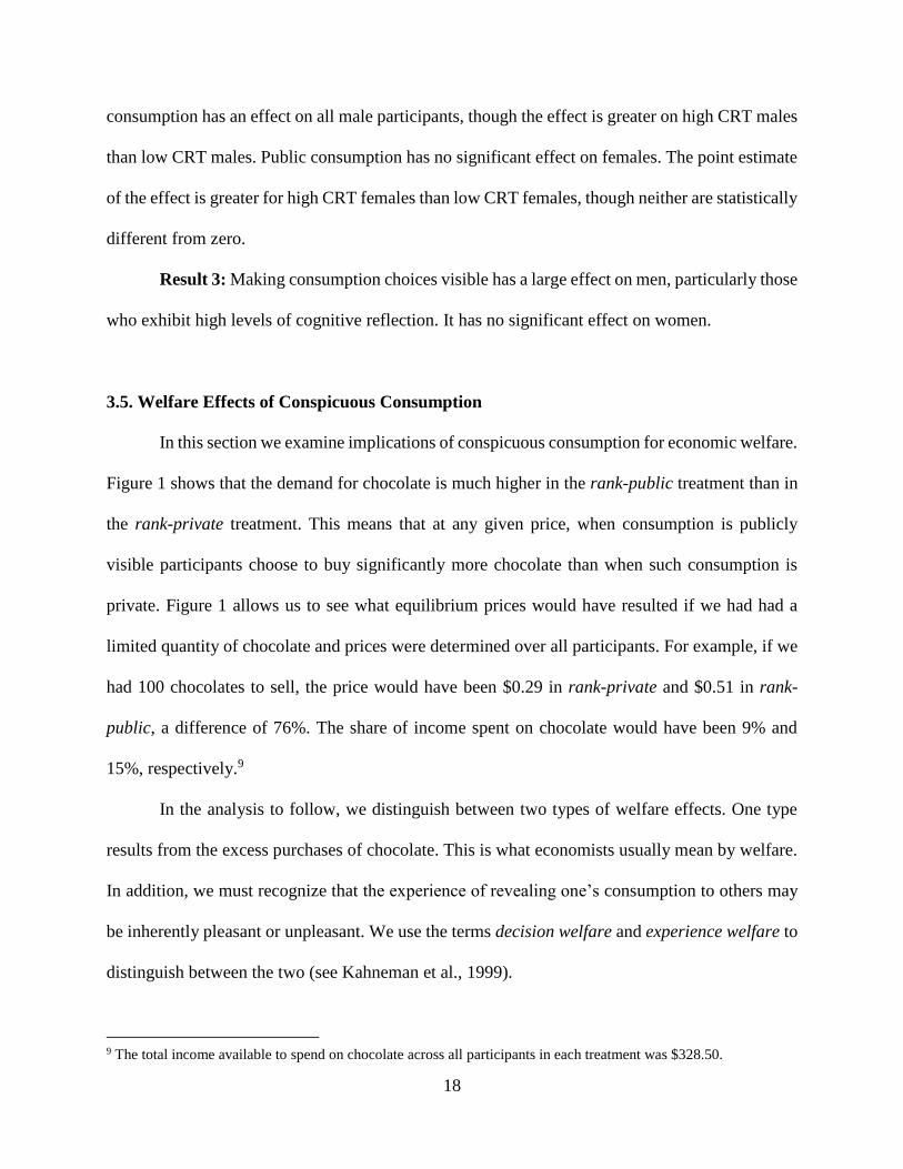
3.5. Welfare Effects of Conspicuous Consumption
In this section we examine implications of conspicuous consumption for economic welfare.
Figure 1 shows that the demand for chocolate is much higher in the rank-public treatment than in
the rank-private treatment. This means that at any given price, when consumption is publicly
visible participants choose to buy significantly more chocolate than when such consumption is
private. Figure 1 allows us to see what equilibrium prices would have resulted if we had had a
limited quantity of chocolate and prices were determined over all participants. For example, if we
had 100 chocolates to sell, the price would have been $0.29 in rank-private and $0.51 in rank-
public, a difference of 76%. The share of income spent on chocolate would have been 9% and
15%, respectively.9
In the analysis to follow, we distinguish between two types of welfare effects. One type
results from the excess purchases of chocolate. This is what economists usually mean by welfare.
In addition, we must recognize that the experience of revealing one’s consumption to others may
be inherently pleasant or unpleasant. We use the terms decision welfare and experience welfare to
distinguish between the two (see Kahneman et al., 1999).
9 The total income available to spend on chocolate across all participants in each treatment was $328.50.
19
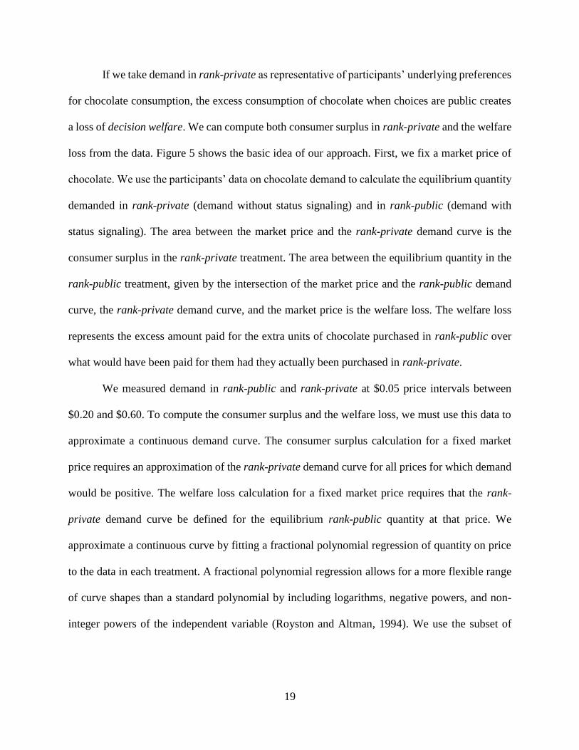
If we take demand in rank-private as representative of participants’ underlying preferences
for chocolate consumption, the excess consumption of chocolate when choices are public creates
a loss of decision welfare. We can compute both consumer surplus in rank-private and the welfare
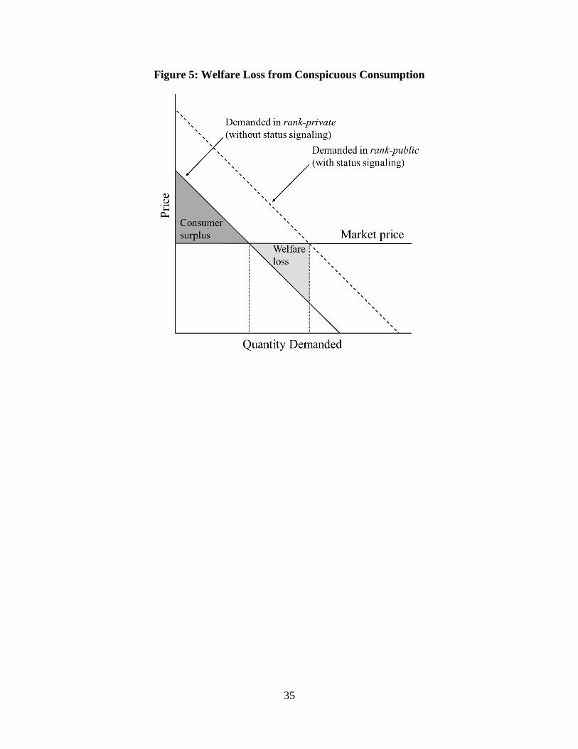
loss from the data. Figure 5 shows the basic idea of our approach. First, we fix a market price of
chocolate. We use the participants’ data on chocolate demand to calculate the equilibrium quantity
demanded in rank-private (demand without status signaling) and in rank-public (demand with
status signaling). The area between the market price and the rank-private demand curve is the
consumer surplus in the rank-private treatment. The area between the equilibrium quantity in the
rank-public treatment, given by the intersection of the market price and the rank-public demand
curve, the rank-private demand curve, and the market price is the welfare loss. The welfare loss
represents the excess amount paid for the extra units of chocolate purchased in rank-public over
what would have been paid for them had they actually been purchased in rank-private.
We measured demand in rank-public and rank-private at $0.05 price intervals between
$0.20 and $0.60. To compute the consumer surplus and the welfare loss, we must use this data to
approximate a continuous demand curve. The consumer surplus calculation for a fixed market
price requires an approximation of the rank-private demand curve for all prices for which demand
would be positive. The welfare loss calculation for a fixed market price requires that the rank-
private demand curve be defined for the equilibrium rank-public quantity at that price. We
approximate a continuous curve by fitting a fractional polynomial regression of quantity on price
to the data in each treatment. A fractional polynomial regression allows for a more flexible range
of curve shapes than a standard polynomial by including logarithms, negative powers, and non-
integer powers of the independent variable (Royston and Altman, 1994). We use the subset of
20
powers from the set {x-2, x-1, x-1/2, ln(x), x1/2, x1, x2, x3} that maximizes the likelihood of the model
to construct the curves.
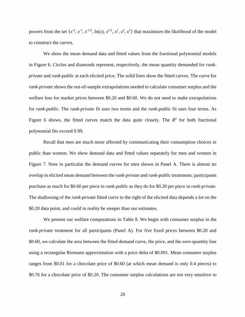
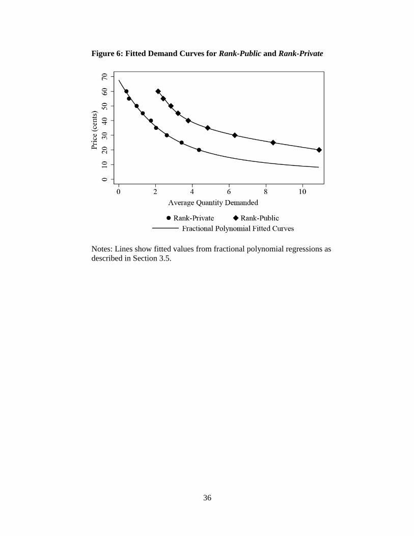
We show the mean demand data and fitted values from the fractional polynomial models
in Figure 6. Circles and diamonds represent, respectively, the mean quantity demanded for rank-
private and rank-public at each elicited price. The solid lines show the fitted curves. The curve for
rank-private shows the out-of-sample extrapolations needed to calculate consumer surplus and the
welfare loss for market prices between $0.20 and $0.60. We do not need to make extrapolations
for rank-public. The rank-private fit uses two terms and the rank-public fit uses four terms. As
Figure 6 shows, the fitted curves match the data quite closely. The R2 for both fractional
polynomial fits exceed 0.99.
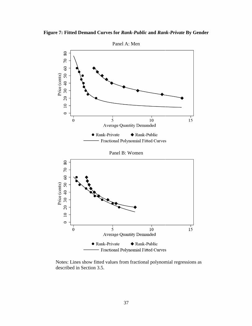
Recall that men are much more affected by communicating their consumption choices in
public than women. We show demand data and fitted values separately for men and women in
Figure 7. Note in particular the demand curves for men shown in Panel A. There is almost no
overlap in elicited mean demand between the rank-private and rank-public treatments: participants
purchase as much for $0.60 per piece in rank-public as they do for $0.20 per piece in rank-private.
The shallowing of the rank-private fitted curve to the right of the elicited data depends a lot on the
$0.20 data point, and could in reality be steeper than our estimates.
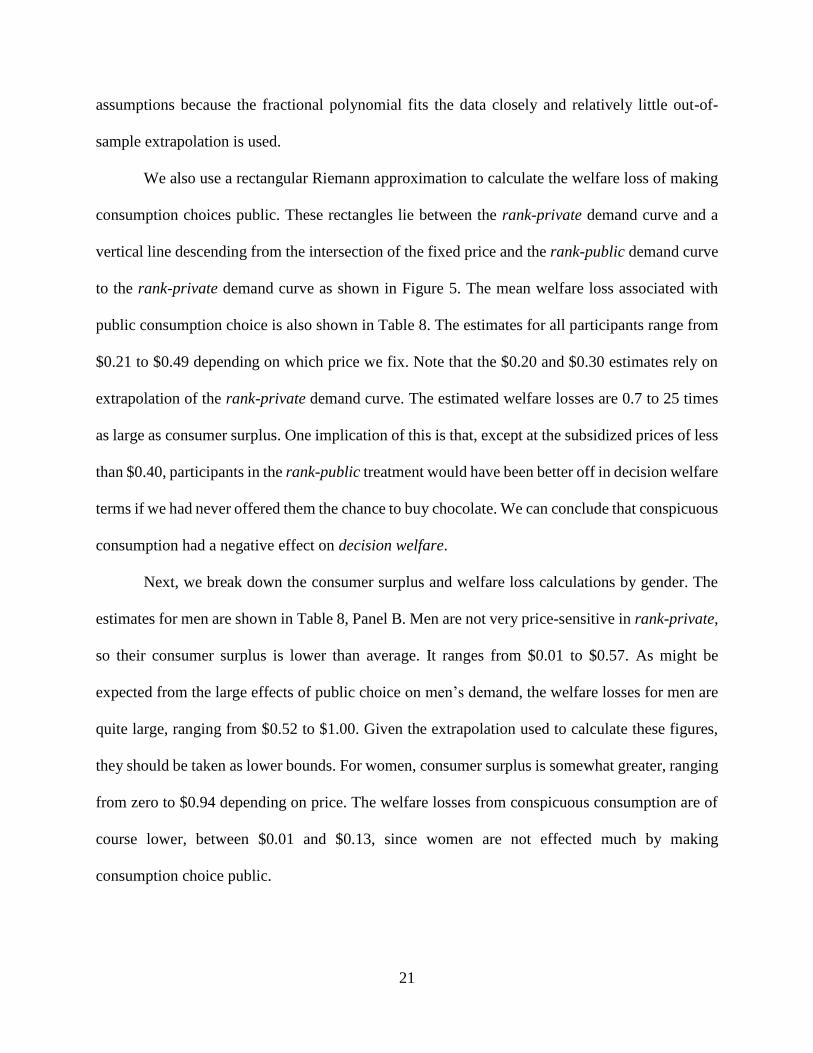
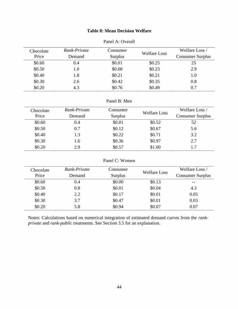
We present our welfare computations in Table 8. We begin with consumer surplus in the
rank-private treatment for all participants (Panel A). For five fixed prices between $0.20 and
$0.60, we calculate the area between the fitted demand curve, the price, and the zero-quantity line
using a rectangular Riemann approximation with a price delta of $0.001. Mean consumer surplus
ranges from $0.01 for a chocolate price of $0.60 (at which mean demand is only 0.4 pieces) to
$0.76 for a chocolate price of $0.20. The consumer surplus calculations are not very sensitive to
21
assumptions because the fractional polynomial fits the data closely and relatively little out-of-
sample extrapolation is used.
We also use a rectangular Riemann approximation to calculate the welfare loss of making
consumption choices public. These rectangles lie between the rank-private demand curve and a
vertical line descending from the intersection of the fixed price and the rank-public demand curve
to the rank-private demand curve as shown in Figure 5. The mean welfare loss associated with
public consumption choice is also shown in Table 8. The estimates for all participants range from
$0.21 to $0.49 depending on which price we fix. Note that the $0.20 and $0.30 estimates rely on
extrapolation of the rank-private demand curve. The estimated welfare losses are 0.7 to 25 times
as large as consumer surplus. One implication of this is that, except at the subsidized prices of less
than $0.40, participants in the rank-public treatment would have been better off in decision welfare
terms if we had never offered them the chance to buy chocolate. We can conclude that conspicuous
consumption had a negative effect on decision welfare.
Next, we break down the consumer surplus and welfare loss calculations by gender. The
estimates for men are shown in Table 8, Panel B. Men are not very price-sensitive in rank-private,
so their consumer surplus is lower than average. It ranges from $0.01 to $0.57. As might be
expected from the large effects of public choice on men’s demand, the welfare losses for men are
quite large, ranging from $0.52 to $1.00. Given the extrapolation used to calculate these figures,
they should be taken as lower bounds. For women, consumer surplus is somewhat greater, ranging
from zero to $0.94 depending on price. The welfare losses from conspicuous consumption are of
course lower, between $0.01 and $0.13, since women are not effected much by making
consumption choice public.
22
We measured experienced welfare by asking participants to rate their overall mood after
the chocolate distribution was completed. They selected an item from a seven-point scale ranging
from “very bad” to “very good”. Experienced welfare is more difficult to measure than decision
welfare because there is no single dimension like money into which behavioral data can be easily
transformed. It is important to note that, for this reason, our measure does not capture all of the
aspects or dimensions of experience that might bear on an understanding of welfare.
We asked participants about their mood after a number of sources of uncertainty had been
resolved, in particular the actual price of chocolate and payouts for the risk aversion and social
preferences measures.10 Participants had also turned in the sheets with their chocolate choices (in
private treatments) or written their chocolate choices on the white board (in public treatments).
Since along with the treatments, the actual price of chocolate, as well as the risk aversion and
social preferences decisions selected for payout varied at the session level, we want to control for
them when looking at how mood varies by treatments. It turns out that mood is positively
correlated with take-home payouts and, perhaps counterintuitively, the realized price of chocolate
(see regressions reported in Table B1 in Appendix B). In the analysis of how participant mood
varies by treatment, we control for the actual price of chocolate, and payouts from risk aversion
and social preferences elicitation.
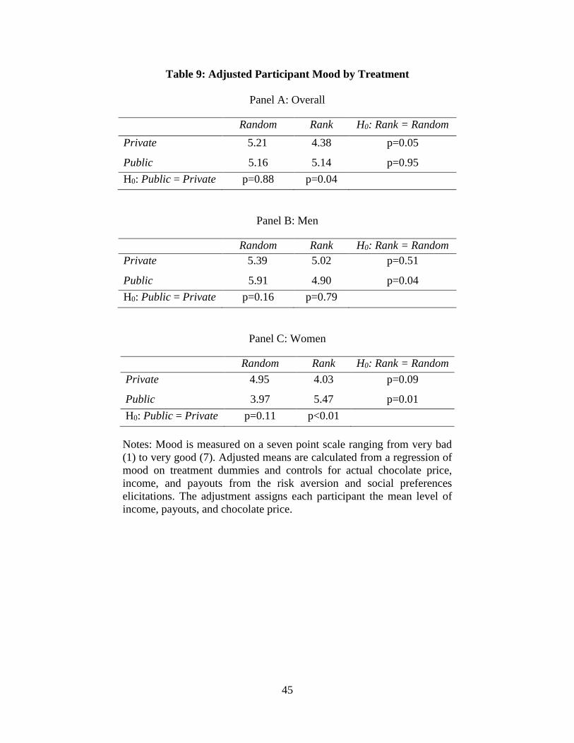
We show the regression-adjusted mean mood of participants by treatment in Table 9.11
There is no sizable or statistically significant difference in mood between participants in random-
private and random-public (Panel A). Recall there was also no difference in demand. The average
10 This was done for two reasons. First, we tried to keep each session under 90 minutes and, given that our experiment
was hand run, we were able to substantially shorten each session by having participants answer the survey
questionnaire while their payoffs were calculated. Second, for a more meaningful measure of the experienced welfare
it was important for participants to experience the actual process of status signaling through purchasing chocolate in
the public treatments. 11 The unadjusted mean mood looks very similar and is shown in Table B2 in Appendix B.
23
mood for both of these groups is just over 5, which corresponds to the response “a little bit good.”
Mood does differ between the treatments in which income is assigned by rank. In rank-private,
the average mood is lower at 4.58. But the average mood in rank-public is 5.14, similar to the
random treatments. The difference of 0.56 points is statistically significant at 8%. The effect of
making consumption public has a positive effect on experienced welfare. It is also worth noting
that when consumption is private, assigning income by rank rather than at random has a negative
effect on overall mood.
We break down participant mood by gender in Panels B and C. Recall that male demand
was most strongly affected by public choice. Interestingly, while the mean experienced welfare
for men of 4.94 in rank-private is lower than 5.28 in rank-public, the difference is only -0.34 and
is not statistically significant. The increase in experienced welfare due to public choice comes
entirely through women. For women, mean experienced welfare in rank-private treatment of 3.56
was 1.73 points lower than the 5.29 in the rank public treatment. Even though public consumption
scarcely changed women’s choices, it did make them feel better. Note that experienced welfare in
the random-private and random-public treatments averaged 4.8, which is much closer to rank-
public than rank-private. It might be more correct to say that when income was assigned by rank,
private consumption made women unhappy to a greater extent than public consumption made them
happy.
In summary, the experiment suggests that pubic consumption causes a loss of decision
welfare by inducing more consumption of chocolate. This loss falls primarily on men, who
accounted for most of the conspicuous consumption. The loss exceeds the consumer surplus of
chocolate consumption by a wide margin, so that rank-public men were worse off in terms of
decision welfare than if they had not been offered a chance to buy chocolate. Moreover, for men,
24
we find no differences in self-reported moods between rank-public and rank-private, suggesting
that the net welfare effect of conspicuous consumption is negative for men. For women, we find
that the decision welfare loss is much smaller and insignificant. Also, for women, we find that
conspicuous choice elevated their mood, suggesting an increase in experienced welfare, which
probably results in positive net welfare effect of conspicuous consumption.
Result 4: Conspicuous consumption has a large negative effect on the decision welfare of
men, who accounted for most of the conspicuous consumption. Conspicuous choice elevated the
mood of female participants, but not of males, likely offsetting their small loss in decision welfare.
The net welfare effect of conspicuous consumption is therefore negative for men and positive for
women.
4. Discussion and Conclusion
Standard economic theory suggests that the utility people derive from the consumption of
goods and services drives demand. Veblen proposed that, in addition to consumption utility,
demand for publicly visible goods is also driven by the social signals they send about those who
purchase them.
We use a controlled experiment to examine whether adding the element of visibility to the
purchase of a good induces conspicuous consumption. Our experiment provides clear evidence
that this happens. Although we are not the first to examine social status motivations using an
experiment, our use of a physical good to measure of conspicuous consumption eliminates
confounds present in previous studies. To the best of our knowledge, the only experimental studies
attempting to find evidence of conspicuous consumption use contributions to charities and social
dilemmas. For example, many laboratory and field experiments have found that recognizing
25
donors by revealing their identities increases donations to charities and contributions to public
good (Andreoni and Petrie, 2004; Soetevent, 2005; Ariely et al., 2009; Karlan and McConnell,
2014; Samek and Sheremeta, 2014). One may be tempted to conclude that this change of behavior
is evidence of conspicuous consumption. However, it is not clear whether such change of behavior
is due to social status (Glazer and Konrad, 1996; Hopkins and Kornienko, 2004), or due to other
factors, such as a desire to be seen as generous (Ariely et al., 2009; Benabou and Tirole, 2006;
Andreoni et al., 2009) or to avoid being seen as stingy (Bracha and Vesterlund, 2013; Samek and
Sheremeta, 2014), or perhaps a purely altruistic desire to set an example for others to follow
(Karlan and McConnell, 2014). The nice feature of our experimental design is that, instead of
giving to a charity or another participant, our participants buy chocolate. Since buying chocolate
provides only private benefit to the person who purchased it, we are able to study conspicuous
consumption without confounding factors of generosity and altruism, which are present in other
studies. Further, since participants did not know the consumption decisions of others, our
experiment isolates the effect of conspicuous consumption from social learning (Grinblatt et al.,
2008).
We manipulated not only the visibility of the consumption good but also the link between
status and income. In human societies, income and status tend to be naturally related to one
another. We show that the linkage of income to status is critical for producing the conspicuous
consumption response to the visibility of one’s choices to others. This rules out the hypothesis that
conspicuous consumption is about signaling one’s income level itself. The necessary conditions
for conspicuous consumption are thus that 1) a good be visible to others and that 2) income be an
indicator of one’s status.
26
Although our data provide support for a hypothesis that status is a significant factor
motivating consumption of visible goods, the relationship between status level and conspicuous
consumption is non-monotonic. Specifically, we find that participants of moderately high and
moderately low status engage in conspicuous consumption more than participants of middle status.
This pattern makes it difficult to infer someone’s status from their chocolate purchases. However,
such non-monotonicities are possible in signaling games when players counter-signal (Spence,
1973; Feltovich et al., 2002).12
In addition to finding direct evidence for conspicuous consumption, we also investigated
the characteristics that mediate the effect. We found that men are significantly more likely to
engage in conspicuous consumption than women. This finding contributes to an extensive
literature on gender differences in behavior (Croson and Gneezy, 2009). A possible explanation
why men engage in conspicuous consumption more than women is that men are more competitive
(Niederle and Vesterlund, 2007). As such, when seen by others, men are more likely to express
their competitiveness through generosity (Pan and Houser, 2011), or conspicuous consumption in
our case.13 Alternatively, women may not care about the particular status attribute studied in our
experiment – rank on a cognitive test – as much as men.
We also found that participants who exhibit high levels of cognitive reflection were more
likely to engage in conspicuous consumption. We suspect that participants with high scorers on
12 Another explanation, consistent with the signaling story, is that the low status participants try to avoid being
recognized as the lowest performers on the test and thus purchase more chocolate. Yet another explanation is that
people who performed poorly on the test might use consumption of chocolate to comfort themselves (although we
find no support for this as low status people do not consume much chocolate in other conditions). 13 Another explanation is that women may be discouraged from public consumption of chocolate, since purchasing a
rich and highly caloric treat in public may have more negative connotations for women than men. Indeed, when income
is allocated randomly, women consume less chocolate in the public condition than when consumption is private (see
Table B3 in Appendix B).
27
cognitive reflection test are better at comprehending the experiment and thus are more sensitive to
treatment manipulations.
Finally, we provided estimates of the impact of conspicuous consumption on economic
welfare. Status-seeking behavior may have significant negative effect on economic outcomes by
leading to more aggressive sabotage in work places (Charness et al., 2013) and overly competitive
behavior in contests (Sheremeta, 2015).14 Our study points a more fundamental negative impact
of conspicuous consumption. When people engage in conspicuous consumption, they purchase
more of a good than they would if consumption was private. This leads to a welfare loss for
participants in the experiment 0.7 to 25 times as large as the baseline surplus, depending on prices.
The loss for men, who were most affected by choosing publicly, was 1.7 to 52 times as large as
the baseline surplus. These losses cannot be offset by non-consumption benefits of status signaling
because, in the equilibrium that emerged in our experiment, status cannot be easily inferred from
consumption patterns. Further, we find that the mood of men in our study was no different under
publicly visible or private choice.15
Our findings have practical implications. The fact that we find people engaging in
conspicuous consumption even though there is a little signaling value of such consumption speaks
to the ongoing debate on whether to tax visible goods used for status signaling (Frank, 1999, 2008).
Although such a policy could be warranted, our results contain a puzzle that we think ought to be
resolved before making such a suggestion. Our participants engaged in conspicuous consumption
even though there were no benefits to offset the decision welfare loss. Why did they do so? One
14 Of course, in some environments status-seeking behavior may be beneficial to economy. For example, status and
social recognition may be used to enhance worker performance (Kosfeld and Neckermann, 2011) or to encourage
donations to charities (Karlan and McConnell, 2014; Samek and Sheremeta, 2014, 2015). 15 In a market setting, conspicuous consumption of goods for which public visibility is an integral property will tend
to raise prices. Depending on the shape of the demand curve, this may amplify or mute the decision welfare effect,
though we expect it will be negative.
28
possibility is that they incorrectly expected there to be signaling in equilibrium. If this was the
case, we would expect conspicuous consumption to diminish in repeated trials. It is also possible
that signaling is not the motivation for conspicuous consumption. Sending a signal in our
experiment was fairly cheap, so participants could engage in counter-signaling. However, given a
large difference in income between the highest ranked and the lowest ranked participants, this is
unlikely to be the case.16 It is also possible that there are other non-consumption, non-signaling
benefits to conspicuous consumption that we did not capture in our mood measure.17 We leave
these questions for future research.
16 In our experiment the highest ranked individuals made almost three times more than the lowest ranked individuals.
So, the highest ranked individuals could have easily out-signaled the lowest ranked individuals and still earn more
cash. 17 Sivanathan and Pettit (2010) argue that individuals increase their demand for status goods when they receive
negative information about themselves. They terms such information a self-threat. The response to such a threat is to
engage in conspicuous consumption in order to restore or defend self-integrity. We can view those participants who
ranked in the bottom third on the quiz as having received negative information about themselves. Table B4 in
Appendix B reports estimation of two regressions for participants in the rank-private and rank-public treatments. The
dependent variable in the first regression is the income share spent on consumption and in the second regression the
dependent variable is mood. The independent variables are the dummies indicating treatment, female, having a test
rank > 8, as well as the interactions. The estimation results show that participants who receive negative information
about themselves (i.e., test rank > 8) spend higher share of income on chocolate. Also, we find that there is no effect
on participant mood for this subgroup. These findings are consistent with an interpretation that low-rank participants
have lower mood if they fail to engage in extra chocolate consumption in the rank-public treatment (although the
evidence is not causal).
29
References
Andreoni, J., & Bernheim, B.D. (2009). Social image and the 50–50 norm: A theoretical and
experimental analysis of audience effects. Econometrica, 77, 1607-1636.
Andreoni, J., & Petrie, R. (2004). Public goods experiments without confidentiality: a glimpse into
fund-raising. Journal of Public Economics, 88, 1605-1623.
Ariely, D., Bracha, A., & Meier, S. (2009). Doing good or doing well? Image motivation and
monetary incentives in behaving prosocially. American Economic Review, 544-555.
Bagwell, L.S., & Bernheim, B.D. (1996). Veblen effects in a theory of conspicuous consumption.
American Economic Review, 86, 349-373.
Benabou, R., & Tirole, J. (2006). Incentives and prosocial behavior. American Economic Review,
99, 544-555.
Bracha, A., & Vesterlund, L. (2013). How low can you go? Charity reporting when donations
signal income and generosity. Working Paper.
Cason, T.N., Masters, W.A., & Sheremeta, R.M. (2010). Entry into winner-take-all and
proportional-prize contests: An experimental study. Journal of Public Economics, 94, 604-
611.
Charles, K.K., Hurst, E., & Roussanov, N. (2009). Conspicuous consumption and race. Quarterly
Journal of Economics, 124, 425-67.
Charness, G., & Rabin, M. (2002). Understanding social preferences with simple tests. Quarterly
Journal of Economics, 117, 817-869.
Charness, G., Masclet, D., & Villeval, M.C. (2013). The dark side of competition for status.
Management Science, 60, 38-55.
Croson, R., & Gneezy, U. (2009). Gender differences in preferences. Journal of Economic
Literature, 47, 448-474.
Dechenaux, E., Kovenock, D., & Sheremeta, R.M. (2015). A survey of experimental research on
contests, all-pay auctions and tournaments. Experimental Economics, 18, 609-669.
Dohmen, T. & Falk, A. (2011). Performance pay and multidimensional sorting: Productivity,
preferences, and gender. American Economic Review, 101, 556-90.
Feltovich, N., Harbaugh, R., & To, T. (2002), Too cool for school? Signaling and
countersignalling. RAND Journal of Economics, 33, 630-649.
Frank, R.H. (1999). Luxury fever: Money and happiness in an era of excess. New York: The Free
Press.
Frank, R.H. (2008). Should public policy respond to positional externalities? Journal of Public
Economics, 92, 1777–1786.
Frederick, S. (2005). Cognitive reflection and decision making. Journal of Economic Perspectives,
19, 25-42.
Glazer, A., & Konrad, K. A. (1996). A signaling explanation for charity. American Economic
Review, 86, 1019-1028.
Grinblatt, M., Keloharju, M., & Ikäheimo, S. (2008). Social influence and consumption: Evidence
from the automobile purchases of neighbors. Review of Economics and Statistics, 90, 735-
753.
Heffetz, O. (2011). A test of conspicuous consumption: Visibility and income elasticities. Review
of Economics and Statistics, 93, 1101-1117.
Holt, C.A., & Laury, S.K. (2002). Risk aversion and incentive effects. American Economic Review,
92, 1644-1655.
30
Hopkins, E., & Kornienko, T. (2004). Running to keep in the same place: Consumer choice as a
game of status. American Economic Review, 94, 1085-1107.
Kahneman, D., Diener, E., & Schwarz, N. (1999). Well-being: The foundations of hedonic
psychology. New York: Russell Sage Found.
Karlan, D., & McConnell, M. A. (2014). Hey look at me: The effect of giving circles on giving.
Journal of Economic Behavior and Organization, 106, 402-412.
Kosfeld, M., & Neckermann, S. (2011). Getting more work for nothing? Symbolic awards and
worker performance. American Economic Journal: Microeconomics, 3, 86-99.
Kuhn, P., Kooreman, P., Soetevent, A., & Kapteyn, A. (2011). The effects of lottery prizes on
winners and their neighbors: Evidence from the Dutch postcode lottery. American
Economic Review, 101, 2226–2247.
Leibenstein, H. (1950). Bandwagon, snob, and Veblen effects in the theory of consumers' demand.
Quarterly Journal of Economics, 64, 183-207.
Niederle, M. & Vesterlund, L. (2007). Do women shy away from competition? Do men compete
too much? Quarterly Journal of Economics, 122, 1067-1101.
Pan, X.S., & Houser, D. (2011). Competition for trophies triggers male generosity. PloS One, 6(4),
e18050.
Ravina, E. (2007). Habit formation and keeping up with the Joneses: Evidence from micro data.
Working paper.
Royston, P., & Altman, D.G. (1994). Regression using fractional polynomials of continuous
covariates: Parsimonious parametric modelling. Applied Statistics, 43, 429-467.
Samek, A.S., & Sheremeta, R.M. (2014). Recognizing contributors: An experiment on public
goods. Experimental Economics, 17, 673-690.
Samek, A.S., & Sheremeta, R.M. (2015). Selective recognition: How to recognize donors to
increase charitable giving. Working Paper.
Seltzer, N. (2009). 1,014 GRE practice questions. Princeton Review.
Sheremeta, R.M. (2015). Impulsive behavior in competition: Testing theories of overbidding in
rent-seeking contests. Working Paper.
Sivanathan N., & Pettit, N.C. (2010). Protecting the self through consumption: Status goods as
affirmational commodities. Journal of Experimental Social Psychology, 46, 564‐570.
Soetevent, A. (2005). Anonymity in giving in a natural context – a field experiment in 30 churches.
Journal of Public Economics, 89, 2301-2323.
Spence, M. (1973). Job market signaling. Quarterly Journal of Economics, 87, 355-374.
Veblen, T. (2009 [1899]). The theory of the leisure class: An economic study in the evolution of
institutions. New York: Macmillan
31
Figure 1: Aggregate Demand Curves by Treatment
Notes: Lines plot total quantity demanded for each potential price of chocolate in
each treatment.
32
Figure 2: Engel Curves by Treatment
Notes: Lines plot the quantity demanded averaged across all nine
potential prices for participants in each treatment. Participants are
binned by six income levels, which correspond to test ranks 1 and 2,
3 and 4, etc.
33
Figure 3: Conspicuous Consumption by Income/Status Level
Notes: Graph shows differences in mean income share spent on
chocolate between the rank-private and rank-public treatments for six
income/status bins. Differences and confidence intervals computed
from a regression of mean income share on bin dummies, a public
choice dummy, and their interactions. Confidence intervals allow for
heteroskedasticity.
34
Figure 4: Conspicuous Consumption Effects by Subgroup
Notes: Graph shows estimated difference in mean quantity
demanded for each subgroup between rank-private and rank-public.
Estimates computed from regression that interacts a public treatment
dummy with dummies for female gender and high CRT and their
interaction. Bars show 95% confidence intervals.
35
Figure 5: Welfare Loss from Conspicuous Consumption
36
Figure 6: Fitted Demand Curves for Rank-Public and Rank-Private
Notes: Lines show fitted values from fractional polynomial regressions as
described in Section 3.5.
37
Figure 7: Fitted Demand Curves for Rank-Public and Rank-Private By Gender
Panel A: Men
Panel B: Women
Notes: Lines show fitted values from fractional polynomial regressions as
described in Section 3.5.
38
Table 1: Treatments
Chocolate choice
Income allocation Private Public
Rank 3 sessions,
36 participants
3 sessions,
36 participants
Random 3 sessions,
36 participants
3 sessions,
36 participants
Table 2: Participant Characteristics
Mean SD Min Max
Female 0.48
Age 19.96 1.88 18 23
White 0.58
Asian 0.25
African-American 0.08
Undergraduate 0.78
Study Economics/Business 0.13
Family Income 141K 116K 20K 400K
Employed 0.42
Average Hours if Employed 11.53 10.10 0 40
CRT Score 1.50 1.18 0 3
GRE Test Score 6.80 5.19 -7 14
Risk Aversion 0.54
Competitive Social Preferences 0.14
Had Chocolate Today/Yesterday 0.49
Last Ate < 5 Hours Ago 0.60
39
Table 3: Mean Quantity Demanded by Treatment
Random Rank
H0: Random
= Rank
Private 1.74 1.94 p=0.82
Public 1.75 4.98 p<0.01
H0: Public = Private p=0.99 p<0.01
Notes: Means for each treatment are computed by averaging over all
potential prices. The tests of the null hypotheses are computed using
a pooled regression of quantity demanded on four treatment dummies.
Tests allow for arbitrary correlation of unobservables at the participant
level.
40
Table 4: Distribution of Quantity Demanded for Each Price
Panel A: Income Assignment Based on Rank
Price
(cents)
Pub.
30th
Priv.
30th
Pub.
50th
Priv.
50th
Pub.
70th
Priv.
70th
Pub.
90th
Priv.
90th
Pub. = Priv.
p-value
20 2 0 5 2 12 4 35 10 0.007
25 1 0 4 1 10 3 21 8 0.004
30 1 0 3 0.5 8 2 20 10 0.007
35 1 0 2 0 7 2 13 6 0.007
40 0 0 1 0 6 1 11 5 0.061
45 0 0 1 0 5 1 10 3 0.037
50 0 0 1 0 4 1 9 4 0.035
55 0 0 1 0 3 0 8 3 0.003
60 0 0 0.5 0 3 0 8 1 0.003
Panel B: Income Assignment is Random
Price
(cents)
Pub.
30th
Priv.
30th
Pub.
50th
Priv.
50th
Pub.
70th
Priv.
70th
Pub.
90th
Priv.
90th
Pub. = Priv.
p-value
20 1 0 4 1 6 4 10 10 0.103
25 0 0 3 0 5 2 8 8 0.048
30 0 0 1 0 3 1 5 8 0.176
35 0 0 0 0 2 1 4 8 0.296
40 0 0 0 0 1 1 4 5 0.476
45 0 0 0 0 1 0 2 4 0.310
50 0 0 0 0 1 0 2 3 0.207
55 0 0 0 0 1 0 2 2 0.365
60 0 0 0 0 0 0 2 2 0.337
Notes: P-values are from Wilcoxon tests of the equalities of distributions.
41
Table 5: Effects of Visibility on Demanded
Quantity demanded (1) (2)
Public 0.01 -0.72
(0.69) (0.90)
Rank 0.19 0.10
(0.82) (0.90)
Public × Rank 3.04** 3.49**
(1.29) (1.42)
Female 0.93
(0.74)
High CRT 1.33*
(0.76)
Risk Aversion 0.93
(0.65)
Competitive Preferences -1.19
(1.55)
Ate Chocolate Recently 1.41*
(0.78)
Ate Recently -1.22**
(0.61)
Age 21+ 0.04
(0.84)
White -0.13
(0.80)
African-American -1.96**
(0.93)
Undergraduate 0.51
(0.84)
Family Income > $120K 0.01
(0.67)
Employed 0.42
(0.70)
Constant 1.75*** 0.29
(0.62) (1.68)
Adjusted R2 0.07 0.11
N 1,296 1,296
Notes: * significant at 0.10, ** significant at 0.05, and *** significant
at 0.01 level. Standard errors allow for arbitrary correlation of
unobservables at the participant level.
42
Table 6: Mediators of Conspicuous Consumption
Quantity demanded (1) (2) (3) (4) (5) (6) (7)
Public 3.04*** 3.17*** 5.93*** 0.61 2.03* 4.11*** 2.74
(1.09) (0.87) (1.28) (1.11) (1.09) (1.02) (2.07)
Public × Female -5.38*** -3.79**
(1.58) (1.71)
Public × High CRT 5.29*** 3.93**
(1.71) (1.92)
Public × Risk Aversion 2.41 1.24
(1.87) (1.74)
Public × Competitive Preferences -5.34** -0.67
(2.54) (2.84)
Female -0.21 2.39* -0.96 -0.19 -0.08 1.09
(1.35) (1.41) (1.25) (1.33) (1.33) (1.38)
High CRT 1.41 1.82* -1.37 1.39 1.31 -0.40
(0.97) (0.94) (1.08) (1.00) (0.98) (1.13)
Risk Aversion 0.99 0.84 0.54 -0.16 0.79 -0.07
(0.85) (0.83) (0.85) (1.19) (0.83) (1.17)
Competitive Preferences -1.32 -1.15 -0.50 -1.15 1.81 -0.11
(2.23) (2.15) (2.13) (2.24) (2.75) (2.81)
Constant 1.94*** 2.68 1.91 4.78** 3.21 1.80 3.86
(0.54) (2.58) (2.39) (2.24) (2.73) (2.51) (2.41)
Adjusted R2 0.06 0.23 0.27 0.26 0.23 0.24 0.29
N 648 648 648 648 648 648 648
Notes: * significant at 0.10, ** significant at 0.05, and *** significant at 0.01 level. Regressions of participant
chocolate choices in the rank-private and rank-public treatments. All columns include test rank dummies.
Standard errors allow for arbitrary correlation of unobservables at the participant level.
43
Table 7: Conspicuous Consumption by Gender and CRT
Quantity demanded (1)
Public 3.50**
(1.64)
Public × Female -4.69**
(1.85)
Public × High CRT 3.27
(2.30)
Public × Female × High CRT 1.82
(3.31)
Female × High CRT 1.75
(3.14)
Female 0.01
(1.70)
High CRT -1.61
(1.77)
Constant 4.95**
(2.24)
Adjusted R2 0.29
N 648
Notes: ** significant at 0.05 level. Regressions of
participant chocolate choices in the rank-private and
rank-public treatments. Includes test rank dummies.
Standard errors allow for arbitrary correlation of
unobservables at the participant level.
44
Table 8: Mean Decision Welfare
Panel A: Overall
Chocolate
Price
Rank-Private
Demand
Consumer
Surplus Welfare Loss
Welfare Loss /
Consumer Surplus
$0.60 0.4 $0.01 $0.25 25
$0.50 1.0 $0.08 $0.23 2.9
$0.40 1.8 $0.21 $0.21 1.0
$0.30 2.6 $0.42 $0.35 0.8
$0.20 4.3 $0.76 $0.49 0.7
Panel B: Men
Chocolate
Price
Rank-Private
Demand
Consumer
Surplus Welfare Loss
Welfare Loss /
Consumer Surplus
$0.60 0.4 $0.01 $0.52 52
$0.50 0.7 $0.12 $0.67 5.6
$0.40 1.3 $0.22 $0.71 3.2
$0.30 1.6 $0.36 $0.97 2.7
$0.20 2.9 $0.57 $1.00 1.7
Panel C: Women
Chocolate
Price
Rank-Private
Demand
Consumer
Surplus Welfare Loss
Welfare Loss /
Consumer Surplus
$0.60 0.4 $0.00 $0.13 --
$0.50 0.8 $0.01 $0.04 4.3
$0.40 2.2 $0.17 $0.01 0.05
$0.30 3.7 $0.47 $0.01 0.03
$0.20 5.8 $0.94 $0.07 0.07
Notes: Calculations based on numerical integration of estimated demand curves from the rank-
private and rank-public treatments. See Section 3.5 for an explanation.
45
Table 9: Adjusted Participant Mood by Treatment
Panel A: Overall
Random Rank H0: Rank = Random
Private 5.21 4.38 p=0.05
Public 5.16 5.14 p=0.95
H0: Public = Private p=0.88 p=0.04
Panel B: Men
Random Rank H0: Rank = Random
Private 5.39 5.02 p=0.51
Public 5.91 4.90 p=0.04
H0: Public = Private p=0.16 p=0.79
Panel C: Women
Random Rank H0: Rank = Random
Private 4.95 4.03 p=0.09
Public 3.97 5.47 p=0.01
H0: Public = Private p=0.11 p<0.01
Notes: Mood is measured on a seven point scale ranging from very bad
(1) to very good (7). Adjusted means are calculated from a regression of
mood on treatment dummies and controls for actual chocolate price,
income, and payouts from the risk aversion and social preferences
elicitations. The adjustment assigns each participant the mean level of
income, payouts, and chocolate price.

46
Appendix A – Instructions for the Rank-Public Treatment
PART 1 – EXERCISE
In this exercise you will be asked to answer three questions. Below are three items that vary in
difficulty. Answer as many as you can.
1. A bat and a ball cost $1.10 in total. The bat costs $1.00 more than the ball.
How much does the ball cost? _____ cents
2. It takes 5 machines 5 minutes to make 5 widgets.
How long does it take 100 machines to make 100 widgets? _____ minutes
3. In a lake, there is a patch of lily pads. Every day, the patch doubles in size. It takes 48 days for
the patch to cover the entire lake.
How long does it take for the patch to cover half of the lake? _____ days
PART 2 – COGNITIVE TEST
You will now take a 30-minute cognitive test containing 20 questions. You may use the margins
of this booklet work out your answer if needed. You may ONLY use pencil, paper, and calculator
provided. No other aids are permitted.
Please use the attached bubble sheet to record your answers. All questions have the following
format:
Who is the current President of the United States?
A. Mitt Romney
B. Bill Clinton
C. Barack Obama
D. George W. Bush
E. David Cameron
To correctly answer this example question, you would fill in bubble C in line 0.
You will gain one point for each correct answer and lose one point for each incorrect answer.
There is no penalty for leaving a question blank. Please try to get as many points as you can.
You will have 30 minutes to work on the questions. You may not be able to finish all the questions
in this time.
COGNITIVE TEST SCORE AND RANK
Your score on the cognitive test is _____
Your rank among today’s test takers is _____/______
This table shows how many dollars you get based on your rank in the cognitive test.
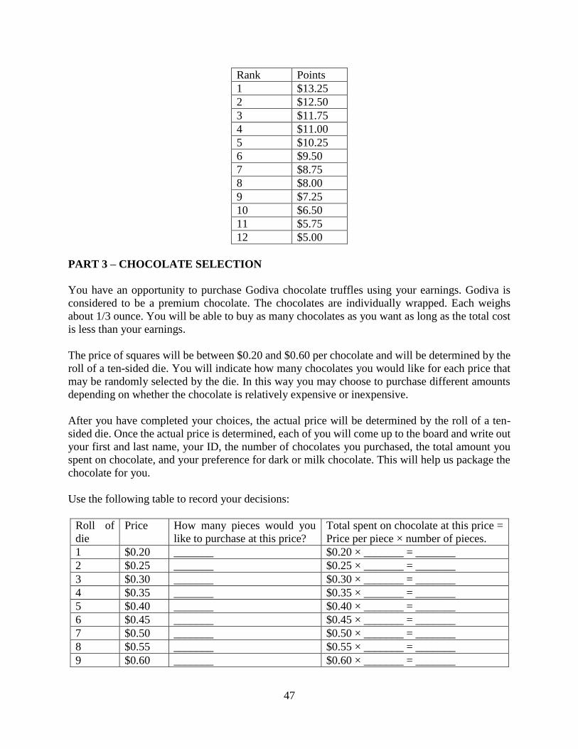
47
Rank Points
1 $13.25
2 $12.50
3 $11.75
4 $11.00
5 $10.25
6 $9.50
7 $8.75
8 $8.00
9 $7.25
10 $6.50
11 $5.75
12 $5.00
PART 3 – CHOCOLATE SELECTION
You have an opportunity to purchase Godiva chocolate truffles using your earnings. Godiva is
considered to be a premium chocolate. The chocolates are individually wrapped. Each weighs
about 1/3 ounce. You will be able to buy as many chocolates as you want as long as the total cost
is less than your earnings.
The price of squares will be between $0.20 and $0.60 per chocolate and will be determined by the
roll of a ten-sided die. You will indicate how many chocolates you would like for each price that
may be randomly selected by the die. In this way you may choose to purchase different amounts
depending on whether the chocolate is relatively expensive or inexpensive.
After you have completed your choices, the actual price will be determined by the roll of a ten-
sided die. Once the actual price is determined, each of you will come up to the board and write out
your first and last name, your ID, the number of chocolates you purchased, the total amount you
spent on chocolate, and your preference for dark or milk chocolate. This will help us package the
chocolate for you.
Use the following table to record your decisions:
Roll of
die
Price How many pieces would you
like to purchase at this price?
Total spent on chocolate at this price =
Price per piece × number of pieces.
1 $0.20 _______ $0.20 × _______ = _______
2 $0.25 _______ $0.25 × _______ = _______
3 $0.30 _______ $0.30 × _______ = _______
4 $0.35 _______ $0.35 × _______ = _______
5 $0.40 _______ $0.40 × _______ = _______
6 $0.45 _______ $0.45 × _______ = _______
7 $0.50 _______ $0.50 × _______ = _______
8 $0.55 _______ $0.55 × _______ = _______
9 $0.60 _______ $0.60 × _______ = _______

48
PART 4 – DECISION PROBLEMS
In this part of the experiment, you will be asked to make a series of choices in decision problems.
How much money you receive will depend partly on chance and partly on the choices you make.
You will see a table with 20 lines. You will state whether you prefer Option A or Option B in each
line. You should think of each line as a separate decision you need to make. At the end of the
experiment, we will draw a card from a deck of cards numbered 1, 2, …., 20. The number on the
card chosen indicates which line in this part will be paid out. You will be paid according to the
option you selected on that line.
In the table, option A always offers a 50% chance to get $10 and a 50% chance to get nothing. To
determine the earnings for people who choose option A, after drawing the card that determines
which line will be paid, we will randomly draw a ball from a bag containing ten orange balls and
ten white balls. That means that when we draw a ball, there is a 50% chance that it is white and a
50% chance that it is orange. If the drawn ball is white and you selected option A in that decision,
you will get the $10, otherwise you will get $0.
Use the following table to record your decisions:
Decision
Number Option A Option B
Choose
A or B
1 $10.00 with 50% chance $0.00 with 50% chance
1,2,3,4,5,6,7,8,9,10,11,
12,13,14,15,16,17,18,1
9,20
$0.50 for sure
2 $10.00 with 50% chance $0.00 with 50% chance
1,2,3,4,5,6,7,8,9,10,11,
12,13,14,15,16,17,18,1
9,20
$1.00 for sure
3 $10.00 with 50% chance $0.00 with 50% chance
1,2,3,4,5,6,7,8,9,10,11,
12,13,14,15,16,17,18,1
9,20
$1.50 for sure
4 $10.00 with 50% chance $0.00 with 50% chance
1,2,3,4,5,6,7,8,9,10,11,
12,13,14,15,16,17,18,1
9,20
$2.00 for sure
5 $10.00 with 50% chance $0.00 with 50% chance
1,2,3,4,5,6,7,8,9,10,11,
12,13,14,15,16,17,18,1
9,20
$2.50 for sure 6 $10.00 with 50% chance $0.00 with 50% chance
1,2,3,4,5,6,7,8,9,10,11,
12,13,14,15,16,17,18,1
9,20
$3.00 for sure
7 $10.00 with 50% chance $0.00 with 50% chance
1,2,3,4,5,6,7,8,9,10,11,
12,13,14,15,16,17,18,1
9,20
$3.50 for sure
8 $10.00 with 50% chance $0.00 with 50% chance
1,2,3,4,5,6,7,8,9,10,11,
12,13,14,15,16,17,18,1
9,20
$4.00 for sure
9 $10.00 with 50% chance $0.00 with 50% chance
1,2,3,4,5,6,7,8,9,10,11,
12,13,14,15,16,17,18,1
9,20
$4.50 for sure
10 $10.00 with 50% chance $0.00 with 50% chance
1,2,3,4,5,6,7,8,9,10,11,
12,13,14,15,16,17,18,1
9,20
$5.00 for sure 11 $10.00 with 50% chance $0.00 with 50% chance
1,2,3,4,5,6,7,8,9,10,11,
12,13,14,15,16,17,18,1
9,20
$5.50 for sure
12 $10.00 with 50% chance $0.00 with 50% chance
1,2,3,4,5,6,7,8,9,10,11,
12,13,14,15,16,17,18,1
9,20
$6.00 for sure
13 $10.00 with 50% chance $0.00 with 50% chance
1,2,3,4,5,6,7,8,9,10,11,
12,13,14,15,16,17,18,1
9,20
$6.50 for sure
14 $10.00 with 50% chance $0.00 with 50% chance
1,2,3,4,5,6,7,8,9,10,11,
12,13,14,15,16,17,18,1
9,20
$7.00 for sure
15 $10.00 with 50% chance $0.00 with 50% chance
1,2,3,4,5,6,7,8,9,10,11,
12,13,14,15,16,17,18,1
9,20
$7.50 for sure
16 $10.00 with 50% chance $0.00 with 50% chance
1,2,3,4,5,6,7,8,9,10,11,
12,13,14,15,16,17,18,1
9,20
$8.00 for sure
17 $10.00 with 50% chance $0.00 with 50% chance
1,2,3,4,5,6,7,8,9,10,11,
12,13,14,15,16,17,18,1
9,20
$8.50 for sure
18 $10.00 with 50% chance $0.00 with 50% chance
1,2,3,4,5,6,7,8,9,10,11,
12,13,14,15,16,17,18,1
9,20
$9.00 for sure
19 $10.00 with 50% chance $0.00 with 50% chance
1,2,3,4,5,6,7,8,9,10,11,
12,13,14,15,16,17,18,1
9,20
$9.50 for sure
20 $10.00 with 50% chance $0.00 with 50% chance
1,2,3,4,5,6,7,8,9,10,11,
12,13,14,15,16,17,18,1
9,20
$10.00 for sure

49
PART 5 – DECISION PROBLEMS
In this part of the experiment, you will be asked to make a series of choices in decision problems.
You will see a table with 12 lines. You will state whether you prefer Option A or Option B in each
line. You should think of each line as a separate decision you need to make. However, only one
line will be the ‘line that counts’ and will be paid out. In particular, at the end of the experiment,
we will draw a card from a deck of cards numbered 1, 2, …., 12. The number on the card chosen
indicates which line in that part will be paid out.
For each line in the table on the next page, please state whether you prefer option A or option B.
Notice that there are a total of 12 lines in the table – you should think of each line as a separate
decision you need to make.
These decisions affect both your own earnings and those of another participant in the experiment
today. All participants have randomly and anonymously being divided into pairs according to
subject number.
Your earnings for the selected line depend on which option you chose: if you chose option A in
that line, you will receive $3.00 and the other participant who will be matched with you will also
receive $3.00. If you chose option B in that line, you and the other participant will receive earnings
as indicated in the table for that specific line. For example, if you chose B in line 2 and this line is
selected for payment, you will receive $3.00 and the other participant will receive $2.00. Similarly,
if you chose B in line 3 and this line is selected for payment, you will receive $3.00 and the other
participant will receive $1.50.
After you have completed all your choices we will draw a card from a deck of cards numbered 1,
2, …., 12 to determine which line is going to be paid. Within each pair, one participant has the
higher and the other the lower subject number. We will then draw a ball from a bag containing 10
orange and 10 white balls. The ball color determines whether the decision of the higher (orange)
or lower (white) subject number will be implemented. If your decision is chosen to be
implemented, then the earnings to you and the other participant will be determined according to
your choice of A or B. If the other participant’s decision is chosen to be implemented, then the
earnings will be determined according to the other participant choice of A or B.
Use the following table to record your decisions:
Decision
Number
Option A
(you, the other participant)
Option B
(you, the other participant)
Choose
A or B
1 $3.00 to you, $3.00 to other $3.00 to you, $2.50 to other
2 $3.00 to you, $3.00 to other $3.00 to you, $2.00 to other
3 $3.00 to you, $3.00 to other $3.00 to you, $1.50 to other
4 $3.00 to you, $3.00 to other $2.50 to you, $2.00 to other
5 $3.00 to you, $3.00 to other $2.50 to you, $1.50 to other 6 $3.00 to you, $3.00 to other $2.50 to you, $1.00 to other
7 $3.00 to you, $3.00 to other $3.00 to you, $3.50 to other
8 $3.00 to you, $3.00 to other $3.00 to you, $4.00 to other

50
9 $3.00 to you, $3.00 to other $3.00 to you, $4.50 to other
10 $3.00 to you, $3.00 to other $3.50 to you, $4.00 to other 11 $3.00 to you, $3.00 to other $3.50 to you, $4.50 to other
12 $3.00 to you, $3.00 to other $3.50 to you, $5.00 to other
After you have completed your decisions, please fill out the bubble sheet attached to this booklet
with your responses for each line, indicating whether you chose A or B.
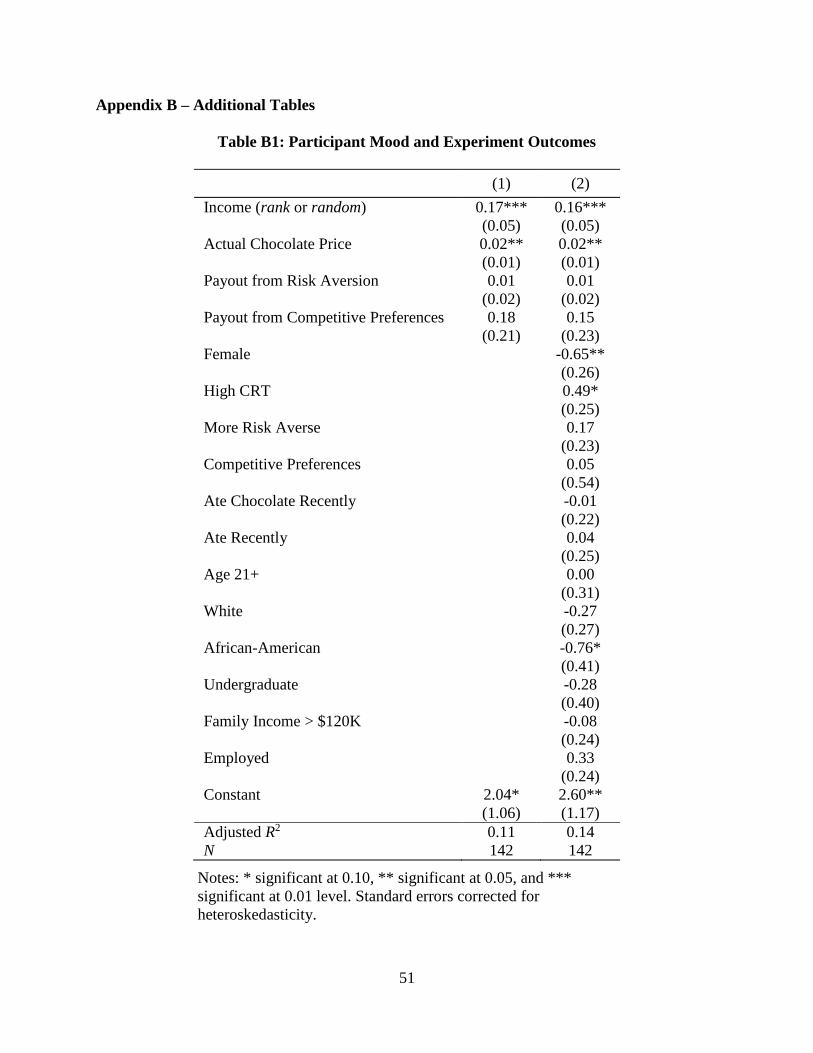
51
Appendix B – Additional Tables
Table B1: Participant Mood and Experiment Outcomes
(1) (2)
Income (rank or random) 0.17*** 0.16***
(0.05) (0.05)
Actual Chocolate Price 0.02** 0.02**
(0.01) (0.01)
Payout from Risk Aversion 0.01 0.01
(0.02) (0.02)
Payout from Competitive Preferences 0.18 0.15
(0.21) (0.23)
Female -0.65**
(0.26)
High CRT 0.49*
(0.25)
More Risk Averse 0.17
(0.23)
Competitive Preferences 0.05
(0.54)
Ate Chocolate Recently -0.01
(0.22)
Ate Recently 0.04
(0.25)
Age 21+ 0.00
(0.31)
White -0.27
(0.27)
African-American -0.76*
(0.41)
Undergraduate -0.28
(0.40)
Family Income > $120K -0.08
(0.24)
Employed 0.33
(0.24)
Constant 2.04* 2.60**
(1.06) (1.17)
Adjusted R2 0.11 0.14
N 142 142
Notes: * significant at 0.10, ** significant at 0.05, and ***
significant at 0.01 level. Standard errors corrected for
heteroskedasticity.
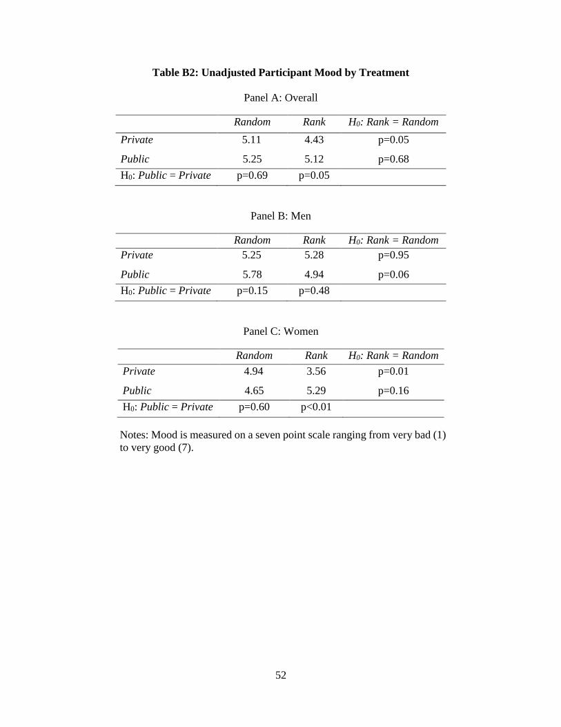
52
Table B2: Unadjusted Participant Mood by Treatment
Panel A: Overall
Random Rank H0: Rank = Random
Private 5.11 4.43 p=0.05
Public 5.25 5.12 p=0.68
H0: Public = Private p=0.69 p=0.05
Panel B: Men
Random Rank H0: Rank = Random
Private 5.25 5.28 p=0.95
Public 5.78 4.94 p=0.06
H0: Public = Private p=0.15 p=0.48
Panel C: Women
Random Rank H0: Rank = Random
Private 4.94 3.56 p=0.01
Public 4.65 5.29 p=0.16
H0: Public = Private p=0.60 p<0.01
Notes: Mood is measured on a seven point scale ranging from very bad (1)
to very good (7).
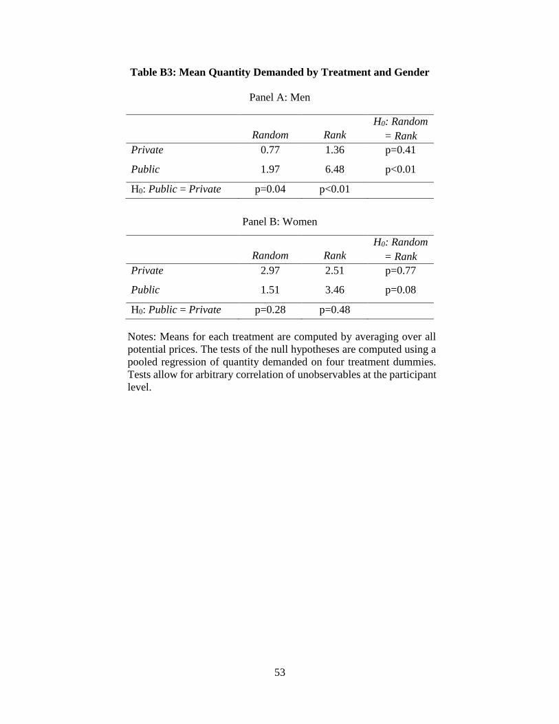
53
Table B3: Mean Quantity Demanded by Treatment and Gender
Panel A: Men
Random Rank
H0: Random
= Rank
Private 0.77 1.36 p=0.41
Public 1.97 6.48 p<0.01
H0: Public = Private p=0.04 p<0.01
Panel B: Women
Random Rank
H0: Random
= Rank
Private 2.97 2.51 p=0.77
Public 1.51 3.46 p=0.08
H0: Public = Private p=0.28 p=0.48
Notes: Means for each treatment are computed by averaging over all
potential prices. The tests of the null hypotheses are computed using a
pooled regression of quantity demanded on four treatment dummies.
Tests allow for arbitrary correlation of unobservables at the participant
level.
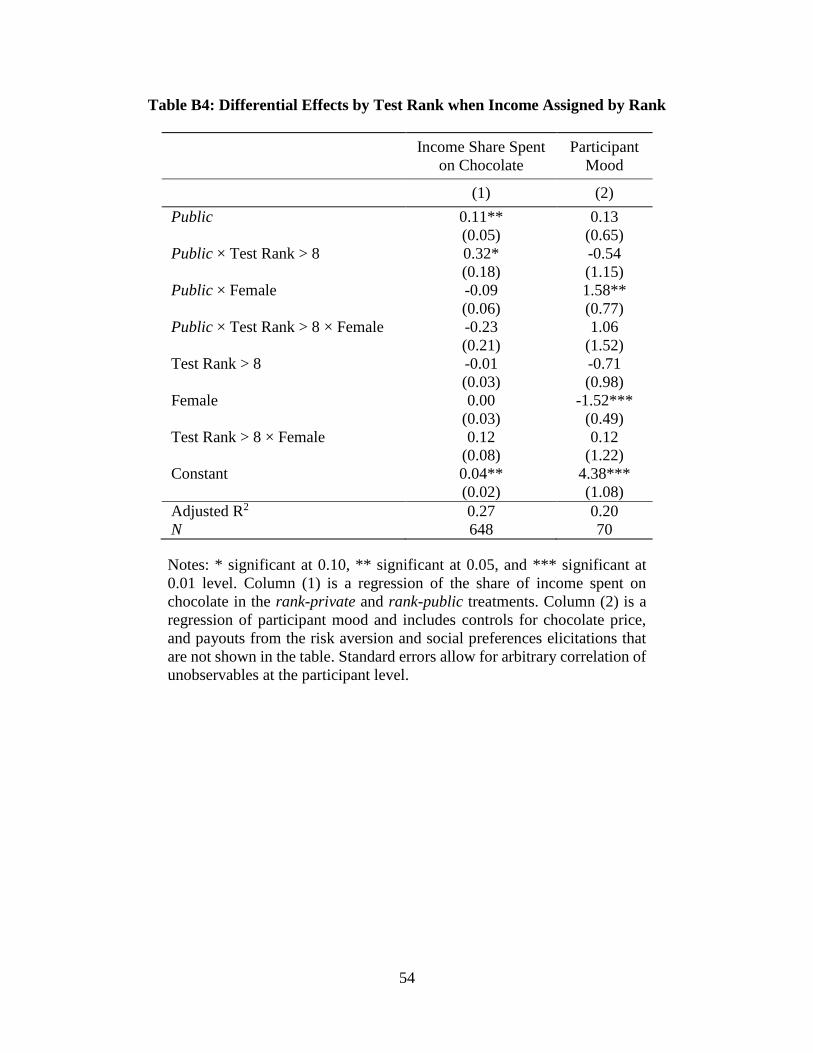
54
Table B4: Differential Effects by Test Rank when Income Assigned by Rank
Income Share Spent
on Chocolate
Participant
Mood
(1) (2)
Public 0.11** 0.13
(0.05) (0.65)
Public × Test Rank > 8 0.32* -0.54
(0.18) (1.15)
Public × Female -0.09 1.58**
(0.06) (0.77)
Public × Test Rank > 8 × Female -0.23 1.06
(0.21) (1.52)
Test Rank > 8 -0.01 -0.71
(0.03) (0.98)
Female 0.00 -1.52***
(0.03) (0.49)
Test Rank > 8 × Female 0.12 0.12
(0.08) (1.22)
Constant 0.04** 4.38***
(0.02) (1.08)
Adjusted R2 0.27 0.20
N 648 70
Notes: * significant at 0.10, ** significant at 0.05, and *** significant at
0.01 level. Column (1) is a regression of the share of income spent on
chocolate in the rank-private and rank-public treatments. Column (2) is a
regression of participant mood and includes controls for chocolate price,
and payouts from the risk aversion and social preferences elicitations that
are not shown in the table. Standard errors allow for arbitrary correlation of
unobservables at the participant level.
Recommended