Department of Mechanical and Aerospace Engineering Technical Report No. 3045, September 1998.Princeton University, Princeton, NJ.
State-Space System Identification with
Identified Hankel Matrix
Ryoung K. Lim 1
Columbia University, New York, NY 10027
Minh Q. Phan 2
Princeton University, Princeton, NJ 08544
Richard W. Longman 3
Columbia University, New York, NY 10027
Abstract
In state-space system identification theory, the Hankel matrix often appears prior
to model realization. Traditionally, one identifies from input-output data the Markov
parameters from which the Hankel matrix is built. This paper examines the strategy
where the Hankel matrix itself is identified from input-output data. Various options are
examined along this direction where the identification of the Hankel matrix can be
carried out directly or indirectly. Advantages and drawbacks associated with each option
are examined and discussed. Extensive evaluation both with simulated and experimental
data indicates that the new approach is effective in detecting the “true” or effective order
of the system, hence it is capable of producing relatively low-dimensional state-space
model. The interactive matrix formulation plays a key role in the development of the
proposed identification technique.
1 Graduate Student, Department of Mechanical Engineering.2 Assistant Professor, Department of Mechanical and Aerospace Engineering, Dissertation Advisor.3 Professor, Department of Mechanical Engineering, Dissertation Co-Advisor.
2
1. Introduction
The problem of state-space system identification has received considerable
attention in recent years. Within the aerospace community, the Eigensystem Realization
Algorithm (ERA),1 an extension of the work of Ho and Kalman,2 has become an
accepted and widely used method. In this or other state-space realization methods 3 the
Hankel matrix plays a critical role because a state-space model can be obtained from a
factorization of the Hankel matrix via its singular value decomposition (SVD) for
example. The Hankel matrix comprises of the Markov parameters arranged in a specific
Toeplitz pattern. Much efforts have been placed on the problem of obtaining the Markov
parameters from input-output data by time or frequency domain approaches.4,5 Once the
Markov parameters are determined, they become entries in the Hankel matrix for state-
space identification.
It is well known that the rank of the Hankel matrix is the order of the system.
With perfect noise-free data, the minimum order realization can be easily obtained by
keeping only the non-zero Hankel singular values. With real or noise-contaminated data,
however, the Hankel matrix tends to be full rank, thus making the problem of
determining a minimum-order state-space model non-trivial. In this case, one would
hope for a significant drop in the singular values that signals the “true” order of the
system, but while this can happen with low-noise simulated data, it rarely happens with
real data. A reduced-order model obtained by retaining only “significant” singular values
tends to be poor in accuracy. Indeed, this issue remains one of the most unsatisfactory

3
discrepancy between what is expected in theory and what is actually observed in practice.
One may argue that real systems are both non-linear and infinite dimensional. While this
is certainly true in many cases it is not to blame in all cases. A common procedure is to
keep all Hankel singular values at the expense of a high-dimensional state-space model
and use a separate post-identification procedure such as model reduction is to reduce the
dimension of the identified model. However, any time model reduction is invoked, some
accuracy is lost. It is preferable to have an identification method that produces a “true”
or effective order model directly in the first place.
While detailed analysis that explains the above phenomenon is difficult because
the relationship between the Hankel matrix and the final state-space realization is quite
non-linear, some heuristic arguments may provide insights into the problem. In the
presence of noise, the identified Markov parameters that are the building blocks of the
Hankel matrix are invariably in error. Since the Hankel matrix has a very specific
Toeplitz pattern, this error pattern is built in the Hankel matrix and subsequent non-linear
decomposition during the realization step does nothing to undo it. Furthermore, the
Markov parameters themselves are usually not directly identified from input-output data,
but computed indirectly via an identified auto-regressive or transfer function model. This
leads to the idea of identifying the Markov parameters directly from input-output data as
done in Refs. 6, 7 through the use of ARMarkov models. In this paper, we go one step
further in trying to identify the Hankel matrix itself directly from input-output data. The
motivation here is that by skipping intermediate steps, an identified Hankel matrix does
not suffer from having the error pattern that is associated with a Hankel matrix that is

4
built from the Markov parameters which are directly or indirectly identified. Since the
Hankel matrix consists of the Markov parameters, an identified Hankel matrix essentially
has the Markov parameters themselves directly identified from input-output data as well.
In this paper we will first provide a generalization of the ARMarkov model
development through the use of interaction matrix. Next, we will develop equations that
allow the Hankel matrix to be identified from input-output data. Several options will be
examined where the Hankel matrix identification is carried out directly, or indirectly, or
both. Following the theoretical development, extensive results using both simulated and
real data will be used to examine the utility of the identified Hankel approach in
comparison with other methods.
2. Auto-Regressive Model with Markov Parameter Coefficients (ARMarkov)
In the following we will derive the ARMarkov models via the use of an
interaction matrix. This development is a generalization of the ARMarkov model first
derived in Ref. 6 for adaptive neural control, and later in Ref. 7 for system identification,
and Ref. 8 for predictive control. Consider an n-th order, r-input, m-output discrete-time
model of a system in state-space format
x k Ax k Bu k
y k Cx k Du k
( ) ( ) ( )
( ) ( ) ( )
+ = += +
1 (1)
By repeated substitution, we have for some p ≥ 0 ,
5
x k p A x k u k
y k x k u k
pp p
p p
( ) ( ) ( )
( ) ( ) ( )
+ = +
= +
C
O T (2)
where u kp( ) and y kp( ) are defined as column vectors of input and output data going p
steps into the future starting with u k( ) and y k( ), respectively,
u k
u k
u k
u k p
y k
y k
y k
y k p
p p( )
( )
( )
( )
, ( )
( )
( )
( )
=+
+ −
=+
+ −
1
1
1
1
M M (3)
For a sufficiently large p, Cp in Eq. (2) is an n × pr controllability matrix, O a pm n×
observability matrix, T a pm pr× Toeplitz matrix of the system Markov parameters,
C O Tpp
pp
A B AB B
C
CA
CA
D
CB D
CAB CB D
CA B CAB CB D
= [ ] =
=
−
−−
1
12
0 0 0
0
0
, , , , , LM
L
O O M
O
M O O O
K
(4)
As long as pm n≥ , it is guaranteed for an observable system that an interaction matrix M
exists such that A Mp + =O 0 . The existence of M ensures that for k ≥ 0 there exists an
expression for x k p( )+ where the state variable is completely eliminated from Eq. (2),

6
x k p M u k My kp p p( ) ( ) ( )+ = +( ) −C T (5)
From the point of view of system identification, Eq. (5) is significant for two reasons. It
is independent of the unknown initial conditions x( )0 , and it is independent of the system
stability. Although we invoke the interaction matrix in this derivation, it needs not be
known nor identified during the course of system identification. To derive the
ARMarkov model, first note that
x k q A x k u kqq q( ) ( ) ( )+ = +C (6)
By shifting the time indices in Eq. (5) back by p time steps, and then substituting it into
Eq. (6) we have for k ≥ p an expression for the state x k q( )+ ,
x k q A M u k p A My k p u kq
p pq
p q q( ) ( ) ( ) ( )+ = +( ) − − − +C T C (7)
Substituting Eq. (7) into y k q Cx k q Du k q( ) ( ) ( )+ = + + + , we arrive at an ARMarkov
model representation,
y k q CA M u k p CA My k p C D u kq
p pq
p q q( ) ( ) ( ) , ( )+ = +( ) − − − +[ ] +C T C 1 (8)
We observe that the expression for y(k + q) involves past p input values from u(k −1) to
u(k − p) , past p output values from y(k −1) to y(k − p) , the present input u(k), and q
7
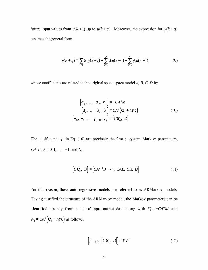
future input values from u(k +1) up to u k q( )+ . Moreover, the expression for y(k + q)
assumes the general form
y k q y k i u k i u k iii
p
ii
p
ii
q
( ) ( ) ( ) ( )+ = − + − + += = =∑ ∑ ∑α β γ
1 1 0
(9)
whose coefficients are related to the original space-space model A, B, C, D by
α α α
β β β
γ γ γ γ
pq
pq
p
q q q
CA M
CA M
C D
, , ,
, , ,
, , ..., , ,
K
K
2 1
2 1
0 1 1
[ ] = −
[ ] = +( )[ ] = [ ]−
C T
C
(10)
The coefficients γi in Eq. (10) are precisely the first q system Markov parameters,
CA Bk , k q= −0 1 1, ,..., , and D,
C D CA B CAB CB Dq
qC , , , , ,[ ] = [ ]−1 L (11)
For this reason, these auto-regressive models are referred to as ARMarkov models.
Having justified the structure of the ARMarkov model, the Markov parameters can be
identified directly from a set of input-output data along with P1 = −CA Mq and
P2 = +( )CA Mq
pC T as follows,
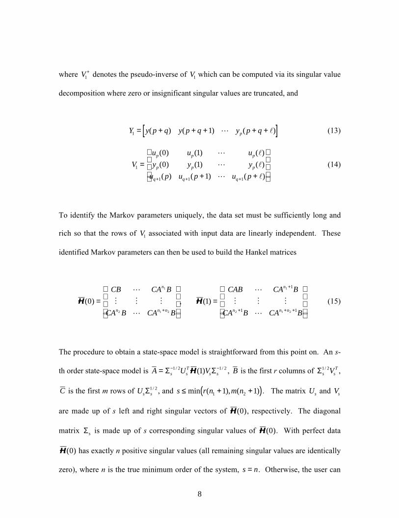
P P1 2 1 1C D YVqC , [ ][ ] = + (12)
8
where V1+ denotes the pseudo-inverse of V1 which can be computed via its singular value
decomposition where zero or insignificant singular values are truncated, and
Y y p q y p q y p qp1 1= + + + + +[ ]( ) ( ) ( )L l (13)
V
u u u
y y y
u p u p u p
p p p
p p p
q q q
1
1 1 1
0 1
0 1
1
=+ +
+ + +
( ) ( ) ( )
( ) ( ) ( )
( ) ( ) ( )
L l
L l
L l
(14)
To identify the Markov parameters uniquely, the data set must be sufficiently long and
rich so that the rows of V1 associated with input data are linearly independent. These
identified Markov parameters can then be used to build the Hankel matrices
H( )0
1
2 1 2
=
+
CB CA B
CA B CA B
n
n n n
L
M M M
L
,
H( )1
1
2 1 2
1
1 1
=
+
+ + +
CAB CA B
CA B CA B
n
n n n
L
M M M
L
(15)
The procedure to obtain a state-space model is straightforward from this point on. An s-
th order state-space model is A U Vs sT
s s= − −Σ Σ1 2 1 21/ /( )H , B is the first r columns of Σs sTV1 2/ ,
C is the first m rows of Us sΣ1 2/ , and s r n m n≤ + +( )min ( ), ( )1 21 1 . The matrix Us and Vs
are made up of s left and right singular vectors of H( )0 , respectively. The diagonal
matrix Σs is made up of s corresponding singular values of H( )0 . With perfect data
H( )0 has exactly n positive singular values (all remaining singular values are identically
zero), where n is the true minimum order of the system, s n= . Otherwise, the user can
9
specify the order of the state-space model by s, the number of Hankel singular values that
he or she wishes to retain. The readers are referred to Ref. 1 for further details.
The ARMarkov model is a generalization of the standard Auto-Regressive model
with eXogenous input (ARX) because it results in an ARX model when q is set to zero in
Eq. (10). The coefficients of the ARX model are related to those of the original state-
space model by the same interaction matrix M. In the ARX model, the Markov
parameters don’t appear explicitly as coefficients but they can be recovered from the
ARX model coefficients.4,5 With ARMarkov models the Markov parameters are
identified directly from input-output data. This is accomplished at the expense of having
to identify additional (extraneous) coefficients α βi i, , i p= 1 2, ,..., . Thus it would be
beneficial to minimize the number of these extraneous terms. The interaction matrix
formulation allows us to do just that because it separates p, pm n≥ , from q which is
number of Markov parameters that one desires to identify.
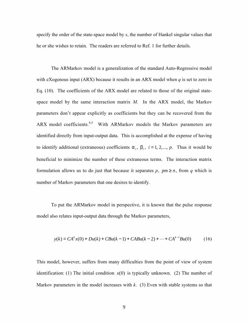
To put the ARMarkov model in perspective, it is known that the pulse response
model also relates input-output data through the Markov parameters,
y k CA x Du k CBu k CABu k CA Buk k( ) ( ) ( ) ( ) ( ) ( )= + + − + − + + −0 1 2 01L (16)
This model, however, suffers from many difficulties from the point of view of system
identification: (1) The initial condition x( )0 is typically unknown. (2) The number of
Markov parameters in the model increases with k. (3) Even with stable systems so that
10
the initial condition response can be neglected when steady-state data is used, one must
keep all “non-zero” Markov parameter coefficients in the model and this number can be
quite high for a lightly damped system. With the ARMarkov model, one can solve for
any desired number of Markov parameters without having to wait for steady-state data
and without concern for the initial condition effect.
3. Hankel-Toeplitz Model
Instead of building the Hankel matrix from the Markov parameters which can be
identified directly via an ARMarkov model, or indirectly via an ARX model, one may
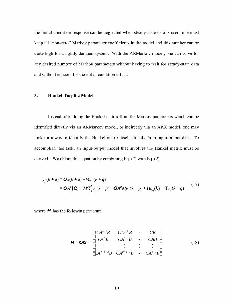
look for a way to identify the Hankel matrix itself directly from input-output data. To
accomplish this task, an input-output model that involves the Hankel matrix must be
derived. We obtain this equation by combining Eq. (7) with Eq. (2),
y k q x k q u k q
A M u k p A My k p u k u k q
p p
qp p
qp q p
( ) ( ) ( )
( ) ( ) ( ) ( )
+ = + + +
= +( ) − − − + + +
O T
O C T O H T (17)
where H has the following structure
H OC= =
− −
−
+ − + − −
q
q q
q q
p q p q p
CA B CA B CB
CA B CA B CAB
CA B CA B CA B
1 2
1
2 3 1
L
L
M M M M
L
(18)

11
Normally, the Hankel matrix is arranged with Markov parameters of increasing order
going from left to right as shown in Eq. (15). All it takes to put H in the standard form is
a simple rearrangement of its elements. Also, for a sufficiently large size H , one can
extract H( )0 and H( )1 for state-space identification. The matrix T is often referred to as
a Toeplitz matrix, hence we call Eq. (17) a Hankel-Toeplitz model.
4. Identification and Construction of Hankel Matrix
In the following we describe three methods by which the Hankel matrix can be
obtained directly or indirectly from a set of input-output data. We then discuss the
advantages or drawbacks associated with each approach
Direct Method
The simplest method is to identify the Hankel matrix directly from input-output
data using Eq. (17). Define A1 = +( )O C TA Mq
p , A2 = −OA Mq , Eq. (17) becomes
y k q
u k p
y k p
u k
u k q
p
p
p
q
p
( )
( )
( )
( )
( )
+ =[ ]
−−
+
A A1 2 H T (19)
Given a set of sufficiently rich input-output data, H can be computed from
A A1 2 2 2H T[ ] = +Y V (20)
12
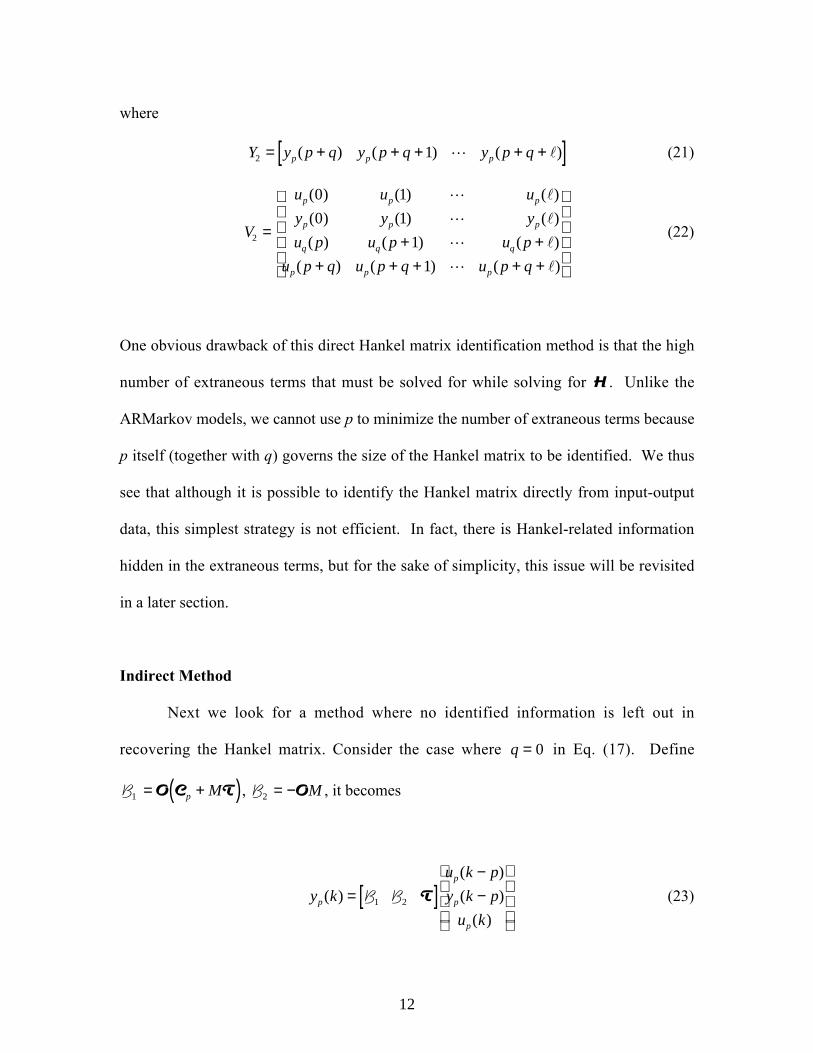
where
Y y p q y p q y p qp p p2 1= + + + + +[ ]( ) ( ) ( )L l (21)
V
u u u
y y y
u p u p u p
u p q u p q u p q
p p p
p p p
q q q
p p p
2
0 1
0 1
1
1
= + ++ + + + +
( ) ( ) ( )
( ) ( ) ( )
( ) ( ) ( )
( ) ( ) ( )
L l
L l
L l
L l
(22)
One obvious drawback of this direct Hankel matrix identification method is that the high
number of extraneous terms that must be solved for while solving for H . Unlike the
ARMarkov models, we cannot use p to minimize the number of extraneous terms because
p itself (together with q) governs the size of the Hankel matrix to be identified. We thus
see that although it is possible to identify the Hankel matrix directly from input-output
data, this simplest strategy is not efficient. In fact, there is Hankel-related information
hidden in the extraneous terms, but for the sake of simplicity, this issue will be revisited
in a later section.
Indirect Method
Next we look for a method where no identified information is left out in
recovering the Hankel matrix. Consider the case where q = 0 in Eq. (17). Define
B1 = +( )O C Tp M , B2 = −OM , it becomes
y k
u k p
y k p
u kp
p
p
p
( )
( )
( )
( )
= [ ]−−
B B1 2 T (23)
13
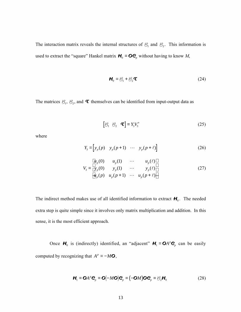
The interaction matrix reveals the internal structures of B1 and B2 . This information is
used to extract the “square” Hankel matrix H OC0 = p without having to know M,
H T0 1 2= +B B (24)
The matrices B1, B2 , and T themselves can be identified from input-output data as
B B1 2 3 3T[ ] = +Y V (25)
where
Y y p y p y pp p p3 1= + +[ ]( ) ( ) ( )L l (26)
V
u u u
y y y
u p u p u p
p p p
p p p
p p p
3
0 1
0 1
1
=+ +
( ) ( ) ( )
( ) ( ) ( )
( ) ( ) ( )
L l
L l
L l
(27)
The indirect method makes use of all identified information to extract H0 . The needed
extra step is quite simple since it involves only matrix multiplication and addition. In this
sense, it is the most efficient approach.
Once H0 is (indirectly) identified, an “adjacent” H O C1 = App can be easily
computed by recognizing that A Mp = − O ,
H O C O O C O OC H1 2 0= = − = −( ) =( )A M Mpp p p B (28)

14
In fact, any other adjacent Hi can be computed in a similar manner,
H O C O O O C O O OC Hip i
p p p
iA M M M M= ( ) = −( ) −( ) = −( ) −( ) = ( )L L B2 0 (29)
Using H0 , H1, … as building blocks, a Hankel matrix of any size can be constructed.
Combined Direct and Indirect Method
In this scheme, the Hankel matrix H0 is identified directly, and all other Hankel
matrices H1, H2 , … are identified indirectly. For convenience we set q p= , and re-visit
the direct method to determine if useful information can be recovered from the
“extraneous” terms. Define C1 = +( )O C TA Mp
p , C2 = −OA Mp , Eq. (17) becomes
y k p
u k p
y k p
u k
u k p
p
p
p
p
p
( )
( )
( )
( )
( )
+ =[ ]
−−
+
C C1 2 0 H T (30)
It is obvious that the Hankel matrix H0 can be directly identified along with C1, C2 , and
T from a set of input-output data as
C C1 2 0 4 4 H T[ ] = +Y V (31)
where

15
Y y p y p y pp p p4 2 2 1 2= + +[ ]( ) ( ) ( )L l (32)
V
u u u
y y y
u p u p u p
u p u p u p
p p p
p p p
p p p
p p p
4
0 1
0 1
1
2 2 1 2
= + ++ +
( ) ( ) ( )
( ) ( ) ( )
( ) ( ) ( )
( ) ( ) ( )
L l
L l
L l
L l
(33)
Making use of the internal structure of the identified parameters as revealed by the
interaction matrix, H O C1 = App can be computed indirectly from C1, C2 , and T as
H T1 1 2= +C C (34)
To compute all other “adjacent” Hankel matrices, we next show that the “even” H2 , H4 ,
… can be computed from H0 and C2 , and the “odd” H3, H5, … can be computed from
H1 and C2 . For example,
H O C O O O C O O OC
O H H
2
2
20 2 0
= ( ) = −( ) −( ) = −( ) −( )
= −( ) =
A M M M M
M
pp p p
C (35)
The last equality holds because C22= − = − −( ) = −( )O O O OA M M M Mp . Similarly,
H O C O O O C O O O C
O H H
3
3
21 2 1
= ( ) = −( ) −( ) = −( ) −( )= −( ) =
A M M A M M A
M
pp
pp
pp
C (36)

16
By induction, H H/i
i= ( )C2
2
0 for even i = 2 4, , ... and H H/i
i= ( ) −( )C2
1 2
1 for odd
i = 3 5, , ... . Again using H0 , H1, … as building blocks, a Hankel matrix of any size can
be constructed. Thus we see that it is possible to make use of the “extraneous” terms to
recover additional Hankel matrices indirectly. However, high dimensionality in the
identification places this method at a disadvantage when compared with the indirect
method.
5. Illustrations with Simulated and Experimental Data
In this section, we examine the quality of identification results obtained from an
identified Hankel matrix with those from a Hankel matrix that is built from the Markov
parameters. The Markov parameters themselves can be identified indirectly through
auto-regressive or transfer function models by a method such as OKID,4,9,10 or directly
through the use of ARMarkov models. The Observer/Kalman filter Identification
(OKID) algorithm also identifies from input-output data an observer or Kalman filter gain
for observer-based controller design, but this information is not needed in our present
application.
The outcome of each identification method (labeled as Hankel, OKID, or
ARMarkov in the illustrations) is a complete state-space model of the system. With
perfect noise-free data , all methods identify the system exactly, so that difference among
these methods can only be seen with noise-contaminated or real data. It is not uncommon
to have an identification method that works well with simulated data under ideal

17
conditions, but fails to perform with real data which may be affected by non-linearities,
aliasing, poor resolution, among other factors. For this reason, extensive numerical
simulation is used to establish the relative performance pattern among these different
methods, and then real data is used to develop a sense of how well this expected pattern
holds up in practice.
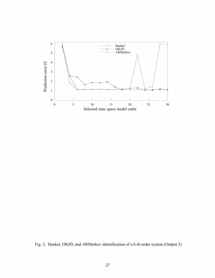
To present a very large amount of results compactly, the combination of model
order and prediction error is used to represent the quality of an identified model. In this
sense, the “best” method is the one that produces the smallest order state-space model
while reproducing the data most accurately. The prediction error is defined as the
difference between the actual output and the reconstructed output of the identified model
when driven by the same input. The norm of this prediction error over the entire data
record is used to indicate the accuracy of the model, and this value is plotted as a function
of model order. For example, if the order increment is 2 then a plot of the norm of the
prediction error versus model order going from 2 to 100 succinctly represents the results
of 50 individual state-space models. Furthermore, to compare different methods, we
have one such plot for each method tested.
Numerical Example
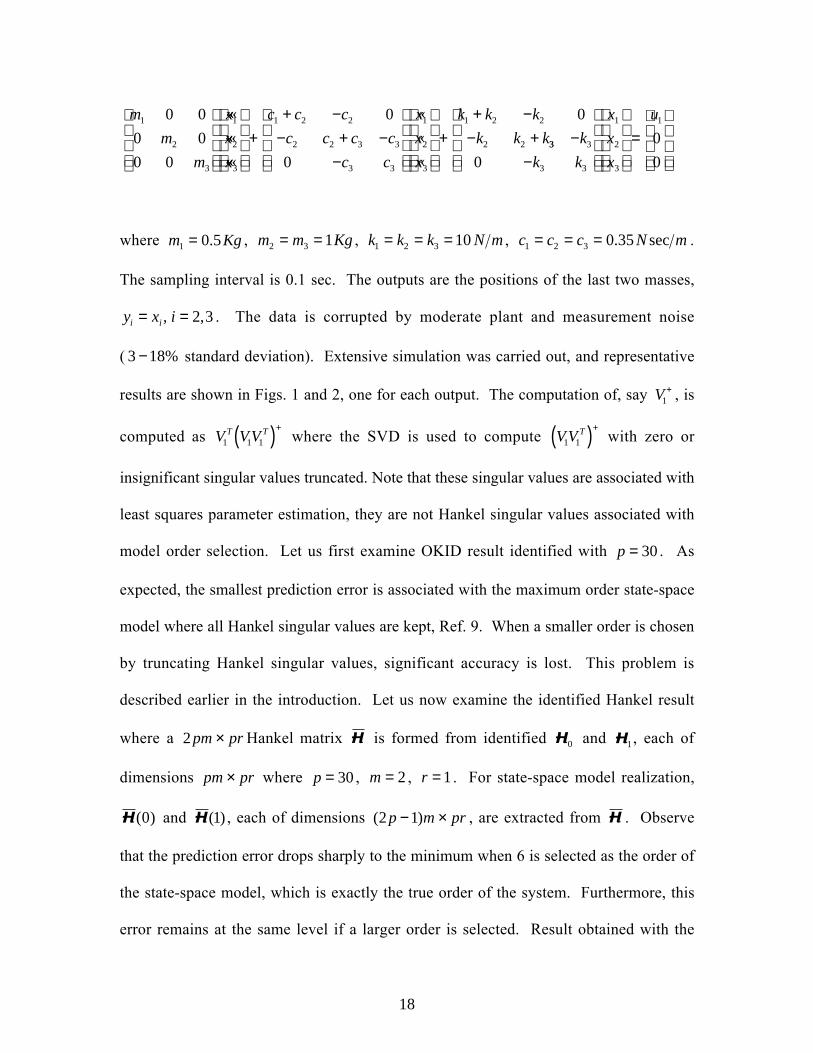
We first examine the performance of each method with simulated data on a 3
degree-of-freedom system,
18
m
m
m
x
x
x
c c c
c c c c
c c
x
x
x
k k k
k k k1
2
3
1
2
3
1 2 2
2 2 3 3
3 3
1
2
3
1 2 2
2 2
0 0
0 0
0 0
0
0
0
++ −
− + −−
++ −
− +««
««
««
«
«
«33 3
3 3
1
2
3
1
0
0
0
−−
=
k
k k
x
x
x
u
where m Kg1 0 5= . , m m Kg2 3 1= = , k k k N m1 2 3 10= = = , c c c N m1 2 3 0 35= = = . sec .
The sampling interval is 0.1 sec. The outputs are the positions of the last two masses,
y x ii i= =, ,2 3 . The data is corrupted by moderate plant and measurement noise
( 3 18− % standard deviation). Extensive simulation was carried out, and representative
results are shown in Figs. 1 and 2, one for each output. The computation of, say V1+ , is
computed as V V VT T1 1 1( )+
where the SVD is used to compute V V T1 1( )+
with zero or
insignificant singular values truncated. Note that these singular values are associated with
least squares parameter estimation, they are not Hankel singular values associated with
model order selection. Let us first examine OKID result identified with p = 30 . As
expected, the smallest prediction error is associated with the maximum order state-space
model where all Hankel singular values are kept, Ref. 9. When a smaller order is chosen
by truncating Hankel singular values, significant accuracy is lost. This problem is
described earlier in the introduction. Let us now examine the identified Hankel result
where a 2 pm pr× Hankel matrix H is formed from identified H0 and H1 , each of
dimensions pm pr× where p = 30 , m = 2 , r = 1 . For state-space model realization,
H( )0 and H( )1 , each of dimensions ( )2 1p m pr− × , are extracted from H . Observe
that the prediction error drops sharply to the minimum when 6 is selected as the order of
the state-space model, which is exactly the true order of the system. Furthermore, this
error remains at the same level if a larger order is selected. Result obtained with the

19
ARMarkov approach where q = 61 Markov parameters are identified with p = 30
follows the same pattern. For a fair comparison, in this and all other test cases, the
number of identified Markov parameters q is chosen so that a Hankel matrix of the same
dimension as an identified Hankel matrix can be formed. At higher model orders the
ARMarkov result is sporadic due to numerical ill-conditioning associated with including
the “smaller” Hankel singular values in Σs−1 2/ that should have been discarded. This is not
necessarily a problem because it may simply indicate that the maximum order has been
reached. Thus we see that both the identified Hankel matrix and the ARMarkov
approaches produce the correct minimum order state-space model directly by Hankel
singular value truncation. The prediction quality of these models is comparable to the
full (high-dimensional) OKID model where all Hankel singular values are kept.
Identification of HST
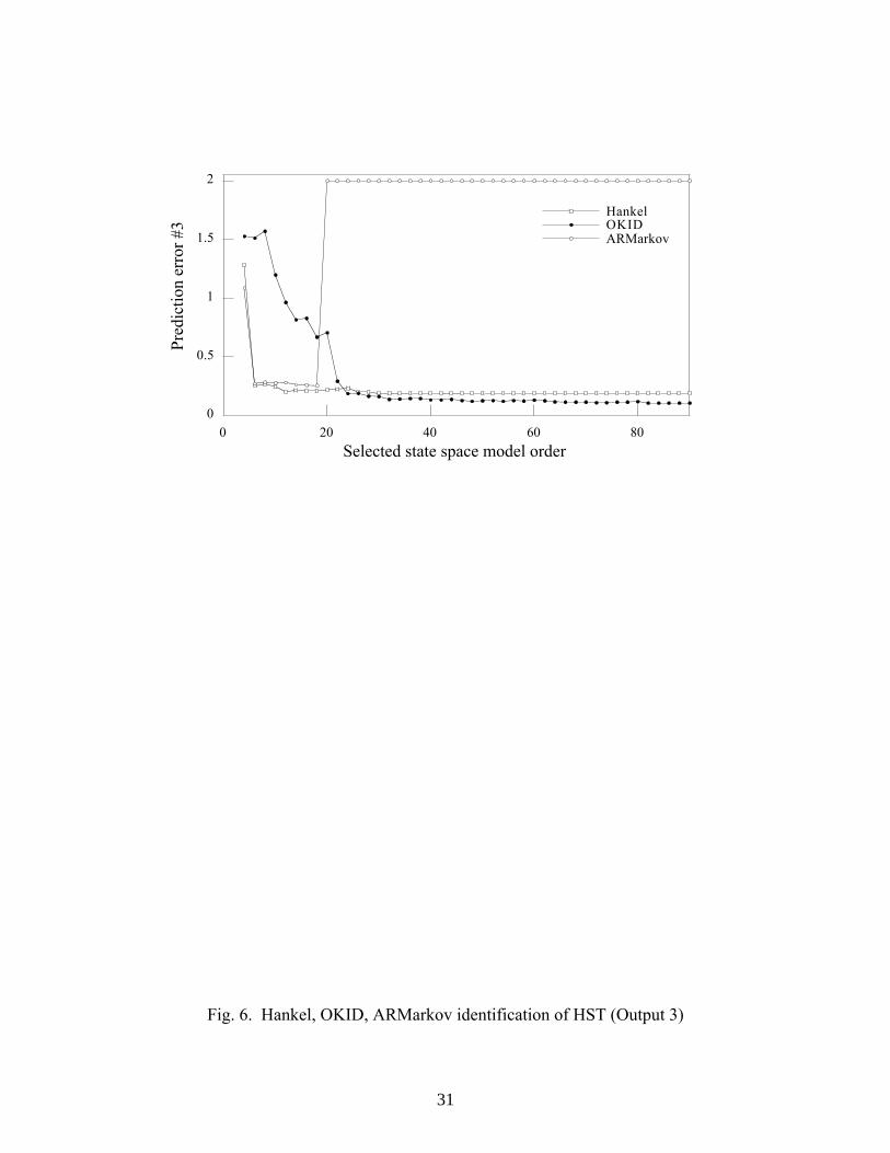
We now examine if the pattern observed in the simulation holds up with real data
through a series of tests. The first test involves a three-input three-output data from the
Hubble Space Telescope (HST) in orbit, Fig. 3. The system is operating in closed-loop,
hence it is highly damped. For this reason the problem of order determination may be
difficult. The HST has six gyros located on the optical telescope assembly which are
used mainly to measure the motion of the primary mirror. The outputs are expressed in
terms of the three angular rates in the vehicle coordinates. The input commands excite
the telescope mirror and structure and they are given in terms of angular acceleration in
the three rotational vehicle axes. The data record is 620 seconds long, and sampled at a
relatively low rate of 10 Hz. The identification results are shown in Figs. 4-6, one for
20
each output. The identified Hankel matrix approach produces a 3-mode model that
reproduces the data quite accurately. This result is in agreement with that obtained with a
more substantial set of data sampled at a higher resolution.9 The ARMarkov result
obtained with q = 61 identified Markov parameters arrives at the same conclusion,
although the result is somewhat more sporadic for higher order models. Indeed, the
highest order that the ARMarkov method can produce with this data is 18, beyond which
the incorporation of additional singular values gives rise to inaccurate results due to the
reason explained earlier. The prediction quality of these low-dimensional models is
similar to the full OKID model for the first two outputs, but a bit worse for the third
output. We thus see that the general pattern observed with simulation data is reproduced
here with this set of experimental data.
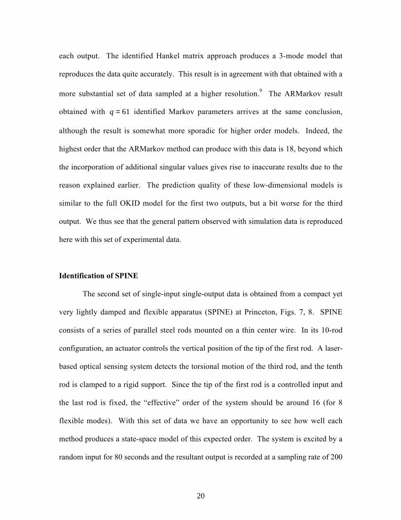
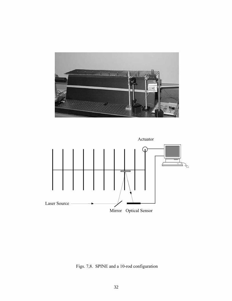
Identification of SPINE
The second set of single-input single-output data is obtained from a compact yet
very lightly damped and flexible apparatus (SPINE) at Princeton, Figs. 7, 8. SPINE
consists of a series of parallel steel rods mounted on a thin center wire. In its 10-rod
configuration, an actuator controls the vertical position of the tip of the first rod. A laser-
based optical sensing system detects the torsional motion of the third rod, and the tenth
rod is clamped to a rigid support. Since the tip of the first rod is a controlled input and
the last rod is fixed, the “effective” order of the system should be around 16 (for 8
flexible modes). With this set of data we have an opportunity to see how well each
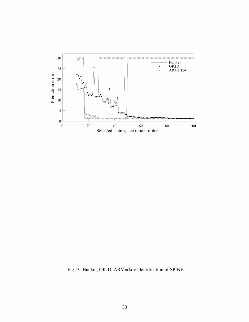
method produces a state-space model of this expected order. The system is excited by a
random input for 80 seconds and the resultant output is recorded at a sampling rate of 200
21
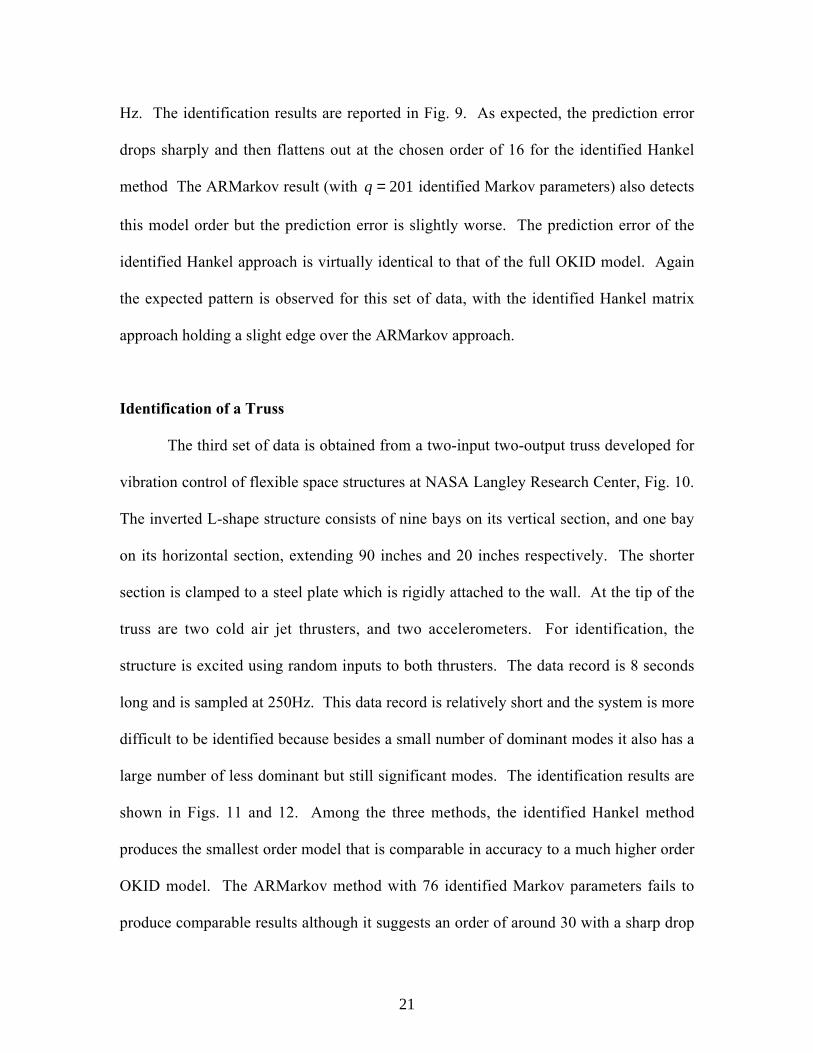
Hz. The identification results are reported in Fig. 9. As expected, the prediction error
drops sharply and then flattens out at the chosen order of 16 for the identified Hankel
method The ARMarkov result (with q = 201 identified Markov parameters) also detects
this model order but the prediction error is slightly worse. The prediction error of the
identified Hankel approach is virtually identical to that of the full OKID model. Again
the expected pattern is observed for this set of data, with the identified Hankel matrix
approach holding a slight edge over the ARMarkov approach.
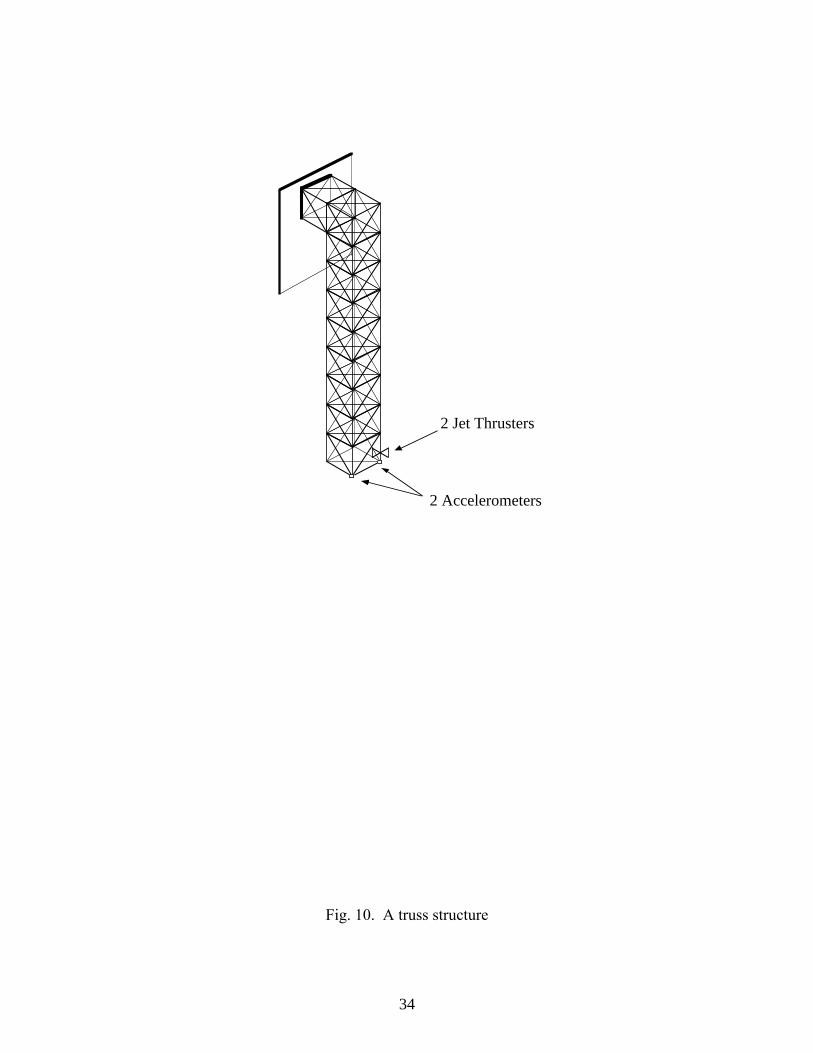
Identification of a Truss
The third set of data is obtained from a two-input two-output truss developed for
vibration control of flexible space structures at NASA Langley Research Center, Fig. 10.
The inverted L-shape structure consists of nine bays on its vertical section, and one bay
on its horizontal section, extending 90 inches and 20 inches respectively. The shorter
section is clamped to a steel plate which is rigidly attached to the wall. At the tip of the
truss are two cold air jet thrusters, and two accelerometers. For identification, the
structure is excited using random inputs to both thrusters. The data record is 8 seconds
long and is sampled at 250Hz. This data record is relatively short and the system is more
difficult to be identified because besides a small number of dominant modes it also has a
large number of less dominant but still significant modes. The identification results are
shown in Figs. 11 and 12. Among the three methods, the identified Hankel method
produces the smallest order model that is comparable in accuracy to a much higher order
OKID model. The ARMarkov method with 76 identified Markov parameters fails to
produce comparable results although it suggests an order of around 30 with a sharp drop

22
in the prediction error. One possible source of difficulty of the ARMarkov method is that
one does not know in advance the number of Markov parameters q that should be solved
for. Since the Markov parameters are the system pulse response samples, they will
eventually converge to zero for a damped system. If q is too small then damping estimate
may be in error. If q is too large then it is possible that many higher order Markov
parameters are essentially zero which need not be identified. While it is not necessary to
solve for all non-zero Markov parameters, the total number depends on the system
stability. This is in contrast to the other two methods where the specification of the order
of the auto-regressive model or the size of the Hankel matrix is essentially a specification
of an upper bound on the order of the system, and this specification is independent of the
system stability. Another distinction between the identified Hankel matrix approach and
the ARMarkov approach is that the former is based on the Hankel-Toeplitz model which
can be thought of as a family of ARMarkov models. Hence for a given set of data, the
Markov parameters in the identified Hankel matrix are required to satisfy a much larger
number of constraints than those in a single ARMarkov model.
In view of the above results and others not reported here due to space limitation, a
number of general observations can be made. OKID is consistent in producing a high
order model with low prediction error. However, model reduction by Hankel singular
value truncation tends to be poor in prediction quality. For this reason, the best strategy
for OKID is to keep the full order model and use a separate procedure for model
reduction. In contrast, the identified Hankel matrix approach is quite consistent in
detecting a true or effective order of the system through Hankel singular value truncation.
23
Thus we can combine these two methods by using OKID to establish the minimum
prediction error level at the expense of high dimensionality, and then use the identified
Hankel matrix method to find a lower dimensional model with the same level of
prediction accuracy as the full OKID model. As a possible third source of confirmation,
the ARMarkov method can be used to corroborate the identified Hankel result in terms of
order confirmation, but this method may not be as consistent as the other two methods.
6. Conclusions
In this paper we examine in details the strategy of using an identified Hankel
matrix for state-space system identification. The standard method is to identify from
input-output data the Markov parameters which are the building blocks of the Hankel
matrix instead of going directly after the Hankel matrix itself. Several options are
examined including schemes where the Hankel matrix is identified directly and indirectly
from input-output data. Advantages and drawbacks associated with each option are
explained. Both simulated and real data are used to perform an extensive evaluation of
this approach. Our results indicate that this approach of identifying the Hankel matrix is
effective in terms of its ability to detect the true or effective order of the system, and to
produce relatively low-dimensional state-space model by Hankel singular value
truncation.
This paper has also shown the utility of the interaction matrix approach in
providing a transparent connection between the state-space model and various input-

24
output models. The interaction matrix serves two primary purposes in this work. First, it
justifies the existence of certain input-output maps that are relevant for the task at hand
(Hankel matrix identification). Second, it reveals the relationship among the identified
coefficients or matrices from which the Hankel matrix can be computed. Interestingly,
this task can accomplished without having to compute explicitly the system-dependent
interaction matrix itself.
References
1. Juang, J.-N., and Pappa, R.S. "An Eigensystem Realization Algorithm for Model
Parameter Identification and Model Reduction," Journal of Guidance, Control, and
Dynamics, Vol. 8, No.5, 1985, pp. 620-627.
2. Ho, B.L. and Kalman, R.E., "Effective Construction of Linear State-variable Models
from Input/Output Data," Proceedings of the Annual Allerton conference on Circuit
and System Theory, Monticello, Illinois, 1965.
3. Chen, C.-T., Linear System Theory and Design, 1984, pp. 232-317.
4. Juang, J.-N., Applied System Identification, Prentice-Hall, Englewood Cliffs, NJ,
1994, pp. 175-252.
5 . Phan, M.Q., Juang, J.-N., and Longman, R.W., “Markov Parameters in System
Identification: Old and New Concepts,” Structronic Systems: Smart Structures,
Devices, and Systems (Part 2), Tzou, H.-S. and Guran, A. (Eds.), World Scientific,
Singapore, 1998, pp. 263-293.

25
6 . Hyland, D.C., "Adaptive Neural Control (ANC) Architecture - a Tutorial,"
Proceedings of the Industry, Government, and University Forum on Adaptive Neural
Control for Aerospace Structural Systems, Harris Corp., Melbourne, FL, August 1993.
7 . Akers, J.C., and Bernstein, D.S., "ARMARKOV Least-Squares Identification,"
Proceedings of the American Control Conference, Albuquerque, NM, June, 1997, pp.
186-190.
8. Lim, R.K., and Phan, M.Q., “Identification of a Multistep-Ahead Observer and Its
Application to Predictive Control.” Journal of Guidance, Control, and Dynamics,
Vol. 20, No. 6, 1997, pp. 1200-1206.
9 . Juang, J.-N., Phan, M.Q., Horta, L.G., and Longman, R.W., "Identification of
Observer/Kalman Filter Markov Parameters: Theory and Experiments," Journal of
Guidance, Control, and Dynamics, Vol. 16, No. 2, 1993, pp. 320-329.
10. Phan, M.Q., Horta, L.G., Juang, J.-N., and Longman, R.W., "Improvement of
Observer/Kalman Filter Identification (OKID) by Residual Whitening," Journal of
Vibrations and Acoustics, Vol. 117, April 1995, pp. 232-239.

26
0
1
2
3
4
5
6
0 5 10 15 20 25 30
HankelOKIDARMarkov
Pred
ictio
n er
ror
#1
Selected state space model order
Fig. 1. Hankel, OKID, and ARMarkov identification of a 6-th order system (Output 1)
27
0
1
2
3
4
5
6
0 5 10 15 20 25 30
Hankel OKIDARMarkov
Pred
ictio
n er
ror
#2
Selected state space model order
Fig. 2. Hankel, OKID, and ARMarkov identification of a 6-th order system (Output 2)

28
Fig. 3. Hubble Space Telescope

29
0
0.5
1
1.5
2
0 20 40 60 80
HankelOKIDARMarkov
Pred
ictio
n er
ror
#1
Selected state space model order
Fig. 4. Hankel, OKID, ARMarkov identification of HST (Output 1)

30
0
0.5
1
1.5
2
0 20 40 60 80
HankelOKIDARMarkov
Pred
ictio
n er
ror
#2
Selected state space model order
Fig. 5. Hankel, OKID, ARMarkov identification of HST (Output 2)
31
0
0.5
1
1.5
2
0 20 40 60 80
HankelOKIDARMarkov
Pred
ictio
n er
ror
#3
Selected state space model order
Fig. 6. Hankel, OKID, ARMarkov identification of HST (Output 3)
32
Actuator
Laser Source
Optical SensorMirror
Figs. 7,8. SPINE and a 10-rod configuration
33
0
5
10
15
20
25
30
0 20 40 60 80 100
HankelOKIDARMarkov
Pred
ictio
n er
ror
Selected state space model order
Fig. 9. Hankel, OKID, ARMarkov identification of SPINE
34
2 Jet Thrusters
2 Accelerometers
Fig. 10. A truss structure

35
0
500
1000
1500
2000
0 10 20 30 40 50 60 70 80
HankelOKIDARMarkov
Pred
ictio
n er
ror
#1
Selected state space model order
Fig. 11. Hankel, OKID, ARMarkov identification of truss (Output 1)

36
0
500
1000
1500
2000
0 10 20 30 40 50 60 70 80
HankelOKIDARMarkov
Pred
ictio
n er
ror
#2
Selected state space model order
Fig. 12. Hankel, OKID, ARMarkov identification of truss (Output 2)
Recommended