
University of Tennessee, Knoxville University of Tennessee, Knoxville
TRACE: Tennessee Research and Creative TRACE: Tennessee Research and Creative
Exchange Exchange
Masters Theses Graduate School
5-2003
State-Space Modeling of the Rigid-Body Dynamics of a Navion State-Space Modeling of the Rigid-Body Dynamics of a Navion
Airplane From Flight Data, Using Frequency-Domain Identification Airplane From Flight Data, Using Frequency-Domain Identification
Techniques. Techniques.
Robert Charles Catterall University of Tennessee - Knoxville
Follow this and additional works at: https://trace.tennessee.edu/utk_gradthes
Part of the Aerospace Engineering Commons
Recommended Citation Recommended Citation Catterall, Robert Charles, "State-Space Modeling of the Rigid-Body Dynamics of a Navion Airplane From Flight Data, Using Frequency-Domain Identification Techniques.. " Master's Thesis, University of Tennessee, 2003. https://trace.tennessee.edu/utk_gradthes/1912
This Thesis is brought to you for free and open access by the Graduate School at TRACE: Tennessee Research and Creative Exchange. It has been accepted for inclusion in Masters Theses by an authorized administrator of TRACE: Tennessee Research and Creative Exchange. For more information, please contact [email protected].

To the Graduate Council:
I am submitting herewith a thesis written by Robert Charles Catterall entitled "State-Space
Modeling of the Rigid-Body Dynamics of a Navion Airplane From Flight Data, Using Frequency-
Domain Identification Techniques.." I have examined the final electronic copy of this thesis for
form and content and recommend that it be accepted in partial fulfillment of the requirements
for the degree of Master of Science, with a major in Aviation Systems.
Ralph Kimberlin, Major Professor
We have read this thesis and recommend its acceptance:
Peter Solies, Frank Collins
Accepted for the Council:
Carolyn R. Hodges
Vice Provost and Dean of the Graduate School
(Original signatures are on file with official student records.)
To the Graduate Council: I am submitting herewith a thesis written by Robert Charles Catterall entitled "State-
Space Modeling of the Rigid-Body Dynamics of a Navion Airplane From Flight
Data, Using Frequency-Domain Identification Techniques.” I have examined the final
electronic copy of this thesis for form and content and recommend that it be accepted
in partial fulfillment of the requirements for the degree of Master of Science, with a
major in Aviation Systems.
Ralph Kimberlin * Major Professor We have read this thesis and recommend its acceptance: Peter Solies * Frank Collins * Accepted for the Council: Anne Mayhew * Vice Provost and Dean of Graduate Studies
(Original signatures are on file with official student records.)
STATE-SPACE MODELING OF THE RIGID-BODY DYNAMICS OF A NAVION AIRPLANE FROM FLIGHT DATA, USING FREQUENCY-DOMAIN IDENTIFICATION TECHNIQUES
A Thesis Presented for the Master of Science
Degree The University of Tennessee, Knoxville
Robert Charles Catterall May 2003
ii
ABSTRACT
State-space models of the open-loop dynamics for the cruise flight condition (V = 90
KCAS) of a modified Navion were extracted from flight data using a frequency-
domain identification method. The identified longitudinal and lateral/directional
models closely match the aircraft’s dynamic response, in both magnitude and phase,
for dissimilar flight data. The identified lateral/directional dimensional stability and
control derivatives, the model parameters, compare well to values obtained from
previous wind tunnel testing. The identified longitudinal derivatives, however, differ
from the wind tunnel results, in some cases significantly. The results for the
longitudinal derivatives are attributed to insufficient excitation of the aircraft,
particularly at the low frequency end (from about 0.2 Hz to 0.6 Hz), and to
differences in the test conditions (most notability, the flight data was for the gear
down configuration, not gear up as in the wind tunnel study). Further investigation,
including additional flight data (preferably from a Navion without fixed gear), is
needed to fully resolve these issues, and necessarily identify the longitudinal
derivatives.
iii
PREFACE
This study is part of ongoing flight-testing research by the Aviation Systems and
Flight Research Department at the University of Tennessee Space Institute. It follows
a 1998 study by Randy Bolding of the “closed-loop” handling qualities of the
Navion’s (N66UT) conventional and fly-by-wire controls using frequency-domain
techniques, entitled: “Handling Qualities Evaluation of a Variable Stability Navion
Airplane (N66UT) Using Frequency-Domain Test Techniques”.
This study involved the planning and execution of a flight test to collect input and
output parameter data for the Navion (N66UT), and data analysis and model
development using CIFER® (Comprehensive Identification from FrEquency
Responses), a system identification and verification software facility. It is intended to
lay the ground work for future efforts aimed at developing a gain scheduling routine
that ties together derivatives identified at select airspeeds to form a [single], variable
coefficient, state-space model of the Navion (N66UT) that is applicable over a wide
airspeed range.
iv
TABLE OF CONTENTS
1. Introduction and Purpose ................................................................................... 1 2. Background .......................................................................................................... 3
2.1 Previous Research........................................................................................... 3 2.2 State-Space Modeling..................................................................................... 4 2.3 Rigid-Body Dynamics .................................................................................... 5 2.4 Identification................................................................................................... 6 2.5 Data Presentation............................................................................................ 8
3. Navion (N66UT) Research Aircraft ................................................................. 10 3.1 Aircraft Description...................................................................................... 10
3.1.1 Aircraft Modifications........................................................................... 10 3.2 Control System ............................................................................................. 14
3.2.1 Cockpit Controls ................................................................................... 14 3.2.2 Moment Controls................................................................................... 14 3.2.3 Normal Force Control ........................................................................... 14
4. Flight Test and Data Aquisition ....................................................................... 15 4.1 Flight Test..................................................................................................... 15
4.1.1 Flight Test Conditions........................................................................... 15 4.1.2 Flight Test Technique............................................................................ 16 4.1.3 Special Flight Test Precautions ............................................................. 18
4.2 Data Aquisition............................................................................................. 18 4.2.1 Cockpit Instrumentation........................................................................ 18 4.2.2 Flight Test Instrumentation ................................................................... 19 4.2.3 Data Acquisition System....................................................................... 19
5. Parameter Identification and Modeling........................................................... 22 5.1 Data Conditioning and Compatability.......................................................... 22 5.2 Spectral Analsis ............................................................................................ 24 5.3 Model Setup.................................................................................................. 26 5.4 Model Structure Determination .................................................................... 29 5.5 Time Domain Verification............................................................................ 30
6. Results ................................................................................................................. 31 6.1 General.......................................................................................................... 31 6.2 Longitudinal Dynamics ................................................................................ 31 6.3 Lateral/Directional Dynamics....................................................................... 37
7. Concluding Remarks ......................................................................................... 43 8. Recommendations .............................................................................................. 44 List of References ...................................................................................................... 45 Appendix .................................................................................................................... 50 Vita............................................................................................................................ 131
v
LIST OF FIGURES
Figure Page
Figure 2-1. Bode and Coherence Plots for Aileron Input (DAIL) to Roll Rate (P), Lateral Accel. (AY), and Roll Angle (PHI). .......................................................... 9
Figure 3-1. Photo of Ryan Navion (N66UT). ............................................................. 11 Figure 3-2. Three-View Drawing of a Navion............................................................ 11 Figure 4-1. Example Frequency Sweep Input (Aileron Control Deflection).............. 16 Figure 5-1. Frequency-Domain Identification/Modeling Methodology. .................... 23 Figure 6-1. Time Histories of the Identified Longitudinal Model for an Elevator
Doublet................................................................................................................. 33 Figure 6-2. Root Locus Diagram of the Identified Longitudinal Model..................... 36 Figure 6-3. Root Locus Diagram of the Comparison Model Based on the Wind
Tunnel Results. .................................................................................................... 36 Figure 6-4. Time Histories of the Identified Lateral/Directional Model for an Aileron
Doublet................................................................................................................. 38 Figure 6-5. Time Histories of the Identified Lateral/Directional Model for a Rudder
Doublet................................................................................................................. 39 Figure 6-6. Root Locus Diagram for the Identified Lateral/Directional Model.......... 42 Figure 6-7. Root Locus Diagram for the Comparison Model Based on the Wind
Tunnel Results. .................................................................................................... 42 Figure A-1. CIFER® Naming Convention for Plots................................................... 51 Figure A-2. Weight and Balance Sheet for Frequency Response Flight Test............. 52 Figure A-3. Photo of DaqBook Installation in N66UT’s Cabin. ................................ 53 Figure A-4. Example Time Histories and Frequency Responses for Two
Concatenated Aileron Frequency Sweeps ........................................................... 55 Figure A-5. LOE Transfer Function Model of Dutch Roll Dynamics. ..................... 106 Figure A-6. Frequency Responses for the Longitudinal Model................................ 111 Figure A-7. Frequency Responses for the Lateral/Directional Model. ..................... 113 Figure A-8. Bode and Coherence Plots of the Relevant Responses to Elevator Input.
............................................................................................................................ 117 Figure A-9. Bode and Coherence Plots of the Relevant Response Parameters to
Aileron Input...................................................................................................... 121 Figure A-10. Bode and Coherence Plots for the Relevant Responses to Elevator Input.
............................................................................................................................ 126
vi
LIST OF TABLES
Table Page
Table 3-1. Navion Specifications. ............................................................................... 12 Table 4-1. Test Matrix................................................................................................. 17 Table 4-2. Measured Input and Output Parameters..................................................... 20 Table 5-1. Parameters Removed During Initial Model Setup..................................... 27 Table 5-2. Frequency Ranges for Selected Frequency-Response Pairs. ..................... 28 Table 6-1. Identified Longitudinal Dimensional Derivatives. .................................... 34 Table 6-2. Longitudinal Dynamic Stability Modes for the Identified Longitudinal
Model. .................................................................................................................. 35 Table 6-3. Longitudinal Dynamic Stability Modes for the Comparison Model Based
On the Wind Tunnel Results................................................................................ 35 Table 6-4. Identified Lateral/Directional Dimensional Derivatives............................ 40 Table 6-5. Lateral/Directional Dynamic Stability Modes for the Identified Model. .. 41 Table 6-6. Lateral/Directional Dynamic Stability Modes for the Comparison Model
Based on the Wind Tunnel Results. ..................................................................... 41 Table A-1. Input and Output/Response Parameters .................................................... 54 Table A-2. Derivative Values and Associated Costs for the Minimally Parameterized
Longitudinal Model. .......................................................................................... 108 Table A-3. Derivative Values and Associated Costs for the Minimally Parameterized
Lateral/Directional Model.................................................................................. 109 Table A-4. Relevant Longitudinal Dimensional Derivatives.................................... 129 Table A-5. Relevant Lateral/Directional Dimensional Derivatives. ......................... 130
vii
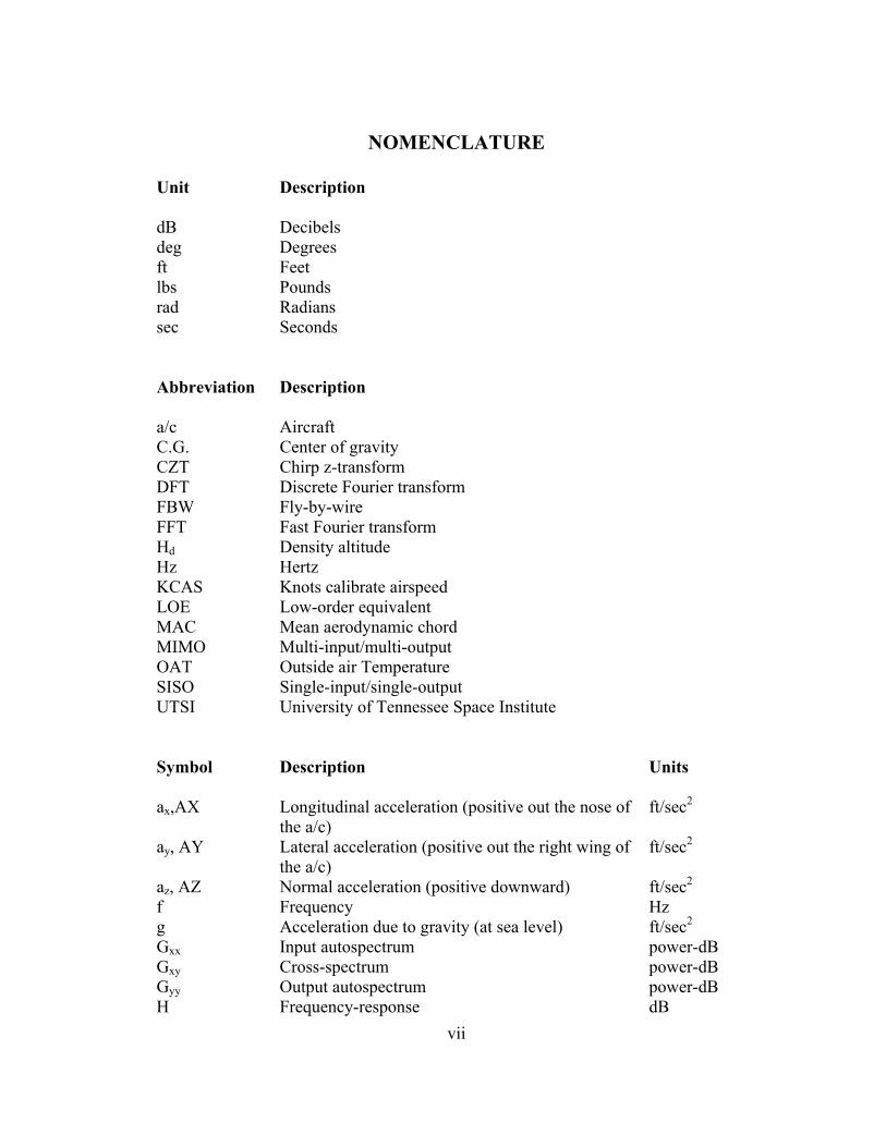
NOMENCLATURE
Unit Description dB Decibels deg Degrees ft Feet lbs Pounds rad Radians sec Seconds Abbreviation Description a/c Aircraft C.G. Center of gravity CZT Chirp z-transform DFT Discrete Fourier transform FBW Fly-by-wire FFT Fast Fourier transform Hd Density altitude Hz Hertz KCAS Knots calibrate airspeed LOE Low-order equivalent MAC Mean aerodynamic chord MIMO Multi-input/multi-output OAT Outside air Temperature SISO Single-input/single-output UTSI University of Tennessee Space Institute Symbol Description Units ax,AX Longitudinal acceleration (positive out the nose of
the a/c) ft/sec2
ay, AY Lateral acceleration (positive out the right wing of the a/c)
ft/sec2
az, AZ Normal acceleration (positive downward) ft/sec2 f Frequency Hz g Acceleration due to gravity (at sea level) ft/sec2 Gxx Input autospectrum power-dB Gxy Cross-spectrum power-dB Gyy Output autospectrum power-dB H Frequency-response dB
NOMENCLATURE (CONT’D)
viii
Hd Density altitude ft l, L Rolling moment ft-lbs m, M Pitching moment ft-lbs n, N Yawing moment ft-lbs p, P Roll rate (positive right-wing down) deg/sec q, Q Pitch rate (positive nose up) deg/sec r, R Yaw rate (positive nose right) deg/sec s Laplace variable 1 S Wing plan form area ft2 u, U Longitudinal speed component ft/sec u Control input vector v, V Lateral speed component ft/sec w, W Normal speed component ft/sec x State vector y Measurement vector β Sideslip angle deg δa, DAIL Aileron surface deflection (positive for right-
aileron tailing edge up, which results in a positive roll rate)
deg
δe, DELE Elevator surface deflection (positive for elevator trailing edge down, which results in a negative pitch rate)
deg
δr, DRUD Rudder surface deflection (positive for rudder trailing edge left, which results in a negative yaw rate)
deg
φ, PHI Bank angle deg θ, THTA Pitch angle deg ψ Heading angle deg ω Frequency rad/sec
1
1. INTRODUCTION AND PURPOSE
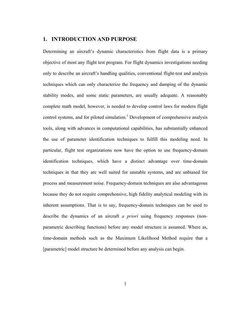
Determining an aircraft’s dynamic characteristics from flight data is a primary
objective of most any flight test program. For flight dynamics investigations needing
only to describe an aircraft’s handling qualities, conventional flight-test and analysis
techniques which can only characterize the frequency and damping of the dynamic
stability modes, and some static parameters, are usually adequate. A reasonably
complete math model, however, is needed to develop control laws for modern flight
control systems, and for piloted simulation.1 Development of comprehensive analysis
tools, along with advances in computational capabilities, has substantially enhanced
the use of parameter identification techniques to fulfill this modeling need. In
particular, flight test organizations now have the option to use frequency-domain
identification techniques, which have a distinct advantage over time-domain
techniques in that they are well suited for unstable systems, and are unbiased for
process and measurement noise. Frequency-domain techniques are also advantageous
because they do not require comprehensive, high fidelity analytical modeling with its
inherent assumptions. That is to say, frequency-domain techniques can be used to
describe the dynamics of an aircraft a priori using frequency responses (non-
parametric describing functions) before any model structure is assumed. Where as,
time-domain methods such as the Maximum Likelihood Method require that a
[parametric] model structure be determined before any analysis can begin.
2
The Navion (N66UT) was selected for this investigation due to its availability as an
instrumented test aircraft, and because derivative estimates determined from previous
wind tunnel testing were available for comparison.
The purpose of this study is to create a 6-DOF state-space derivative model of the
rigid-body dynamics for the Navion (N66UT) from flight data, using frequency-
domain identification techniques.
3
2. BACKGROUND
2.1 PREVIOUS RESEARCH
Scientific interest in describing an aircraft’s dynamic behavior in terms of stability
and control derivates data dates back to reports published by the National Advisory
Committee on Aeronautics (NACA) in the early 1920’s.2 Research involving
frequency-response identification is not new either. In fact, the earliest reported
research of frequency-response identification of aircraft dynamics from flight data
was conducted in 1945 at the Cornell Aeronautical Laboratory.3 For this study, low-
order transfer-function models were derived for the B-25J aircraft using a least-
squares fit of frequency-responses extracted from steady-state sine-wave inputs.
Comprehensive surveys of identification research conducted during the 1950’s,
1960’s and early 1970’s can be found in Reference [3]. More recent frequency-
domain identification efforts are described in References [4], [5] and [6] in which
transfer-function and 6-DOF rigid-body models of various helicopters and tilt-rotors
are derived using CIFER®, the frequency-domain identification analysis software
used by this study.
The Navion has also been used for a number of research efforts. Of particular
relevance to this study are three (3) dynamics studies conducted at Princeton
University—Princeton was the previous owner of this study’s test aircraft—in the
early 1970’s. The first study compared the non-dimensional aerodynamic parameters
obtained from various analytical measurements, wind-tunnel testing, and flight-test
4
data.7 That study found large differences between the wind-tunnel and flight-test
values. The second study extracted non-dimensional aerodynamic parameters from
flight data using a maximum-likelihood minimum-variance technique.8 Results from
the study showed that the values of the parameters were affected by the data and math
model used during the extraction process. The third study compared the longitudinal
derivatives estimated from several different parameter identification methods.9 The
study concluded that the type of identification method only weakly affected the
estimated short-period dynamics, and that results for the aerodynamic coefficients
were dependant on the type of math model and the type of test data. The study further
showed that the Navion has stick-fixed longitudinal stability for angles of attack up to
and through stall at 25% MAC, and that power had a small destabilizing effect.
2.2 STATE-SPACE MODELING
State-space modeling is a mathematical characterization of the [coupled] aircraft
dynamics in terms of ordinary linear differential equations with constant coefficients.
The coefficients of the equations are the force and moment (stability and control)
derivatives of the “linearized” equations of motion, as commonly derived using
small-perturbation assumptions. For example, pitching moment is expressed in terms
of the perturbation variables using a Taylor series expansion similar to the form of
Equation 1. The remaining linear velocities and angular rates are similarly expressed.
⋅⋅⋅+∆∂
∂+⋅⋅⋅+∆
∂
∂+∆
∂
∂+∆
∂
∂= p
pMw
wMv
vMu
uMrqpwvuwvuM rea ),,,,,,,,,,,( δδδDDD (1)
5
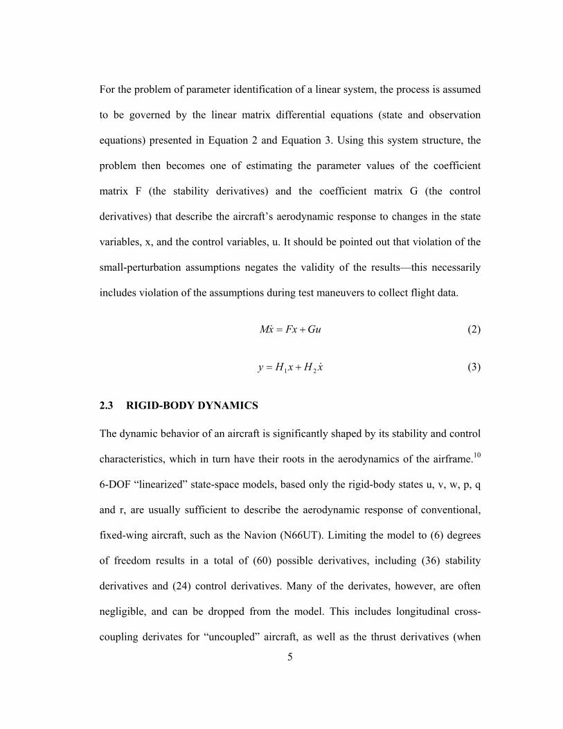
For the problem of parameter identification of a linear system, the process is assumed
to be governed by the linear matrix differential equations (state and observation
equations) presented in Equation 2 and Equation 3. Using this system structure, the
problem then becomes one of estimating the parameter values of the coefficient
matrix F (the stability derivatives) and the coefficient matrix G (the control
derivatives) that describe the aircraft’s aerodynamic response to changes in the state
variables, x, and the control variables, u. It should be pointed out that violation of the
small-perturbation assumptions negates the validity of the results—this necessarily
includes violation of the assumptions during test maneuvers to collect flight data.
GuFxxM +=� (2)
xHxHy C21 += (3)
2.3 RIGID-BODY DYNAMICS
The dynamic behavior of an aircraft is significantly shaped by its stability and control
characteristics, which in turn have their roots in the aerodynamics of the airframe.10
6-DOF “linearized” state-space models, based only the rigid-body states u, v, w, p, q
and r, are usually sufficient to describe the aerodynamic response of conventional,
fixed-wing aircraft, such as the Navion (N66UT). Limiting the model to (6) degrees
of freedom results in a total of (60) possible derivatives, including (36) stability
derivatives and (24) control derivatives. Many of the derivates, however, are often
negligible, and can be dropped from the model. This includes longitudinal cross-
coupling derivates for “uncoupled” aircraft, as well as the thrust derivatives (when
6
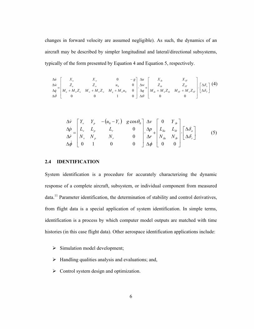
changes in forward velocity are assumed negligible). As such, the dynamics of an
aircraft may be described by simpler longitudinal and lateral/directional subsystems,
typically of the form presented by Equation 4 and Equation 5, respectively.
∆
∆⋅
+++
∆
∆
∆
∆
⋅
+++
−
=
∆
∆
∆
∆
T
e
TwTewe
Te
Te
wqwwwuwu
wu
wu
ZMMZMMZZXX
qwu
uMMZMMZMMuZZ
gXX
qwu
δ
δ
θθ
δδδδ
δδ
δδ
00010000
0
0
0
DDDDD
D
D
D
D
(4)
( )
∆
∆⋅
+
∆
∆
∆
∆
⋅
−−
=
∆
∆
∆
∆
r
a
ra
ra
r
rpv
rpv
rpv
NNLLY
rpv
NNNLLL
gYuYY
rpv
δ
δ
φ
θ
φ
δδ
δδ
δ
00
0
001000
cos 00
D
D
D
D
(5)
2.4 IDENTIFICATION
System identification is a procedure for accurately characterizing the dynamic
response of a complete aircraft, subsystem, or individual component from measured
data.11 Parameter identification, the determination of stability and control derivatives,
from flight data is a special application of system identification. In simple terms,
identification is a process by which computer model outputs are matched with time
histories (in this case flight data). Other aerospace identification applications include:
� Simulation model development;
� Handling qualities analysis and evaluations; and,
� Control system design and optimization.
7
Analytical approaches to identification may be broadly categorized as either time-
domain or frequency-domain methods. Frequency-domain identification methods,
such as the one used for this study, are based on the spectral analysis of the input and
output time histories using FFT techniques. Unlike time-domain methods, frequency-
domain identification does not require high fidelity analytical modeling with its
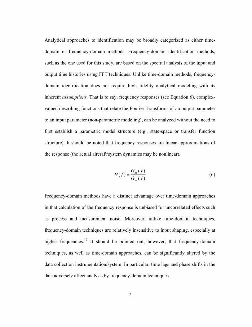
inherent assumptions. That is to say, frequency responses (see Equation 6), complex-
valued describing functions that relate the Fourier Transforms of an output parameter
to an input parameter (non-parametric modeling), can be analyzed without the need to
first establish a parametric model structure (e.g., state-space or transfer function
structure). It should be noted that frequency responses are linear approximations of
the response (the actual aircraft/system dynamics may be nonlinear).
)()(
)(fGfG
fHxx
xy= (6)
Frequency-domain methods have a distinct advantage over time-domain approaches
in that calculation of the frequency response is unbiased for uncorrelated effects such
as process and measurement noise. Moreover, unlike time-domain techniques,
frequency-domain techniques are relatively insensitive to input shaping, especially at
higher frequencies.12 It should be pointed out, however, that frequency-domain
techniques, as well as time-domain approaches, can be significantly altered by the
data collection instrumentation/system. In particular, time lags and phase shifts in the
data adversely affect analysis by frequency-domain techniques.
8
2.5 DATA PRESENTATION
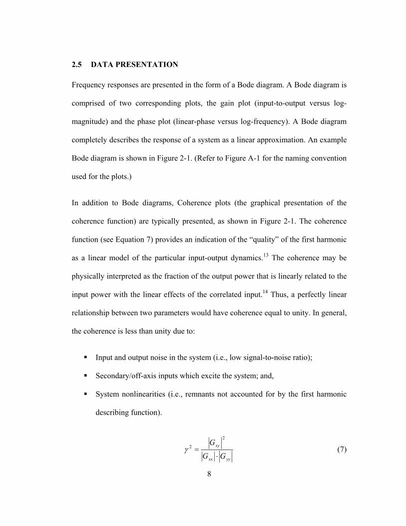
Frequency responses are presented in the form of a Bode diagram. A Bode diagram is
comprised of two corresponding plots, the gain plot (input-to-output versus log-
magnitude) and the phase plot (linear-phase versus log-frequency). A Bode diagram
completely describes the response of a system as a linear approximation. An example
Bode diagram is shown in Figure 2-1. (Refer to Figure A-1 for the naming convention
used for the plots.)
In addition to Bode diagrams, Coherence plots (the graphical presentation of the
coherence function) are typically presented, as shown in Figure 2-1. The coherence
function (see Equation 7) provides an indication of the “quality” of the first harmonic
as a linear model of the particular input-output dynamics.13 The coherence may be
physically interpreted as the fraction of the output power that is linearly related to the
input power with the linear effects of the correlated input.14 Thus, a perfectly linear
relationship between two parameters would have coherence equal to unity. In general,
the coherence is less than unity due to:
� Input and output noise in the system (i.e., low signal-to-noise ratio);
� Secondary/off-axis inputs which excite the system; and,
� System nonlinearities (i.e., remnants not accounted for by the first harmonic
describing function).
yyxx
xy
GG
G
⋅
=
2
2γ (7)
9
Figu
re 2
-1. B
ode
and
Coh
eren
ce P
lots
for
Aile
ron
Inpu
t (D
AIL
) to
Rol
l Rat
e (P
), L
ater
al A
ccel
. (A
Y),
and
Rol
l Ang
le
(PH
I).
Unr
elia
ble
Dat
a
10
3. NAVION (N66UT) RESEARCH AIRCRAFT
3.1 AIRCRAFT DESCRIPTION
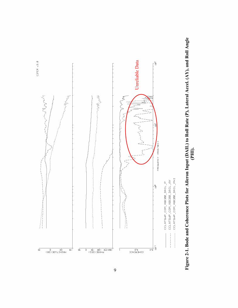
The research aircraft is a modified Navion (Registration Number N66UT; Serial
Number NAV-42013) manufactured by Ryan Aeronautical Company of San Diego,
California. It is a low-wing, four-place airplane, powered by a single air-cooled
engine with tricycle landing gear. Its fuselage is an all-metal one-piece semi-
monocoque structure; the empennage is a cantilever monoplane type with a
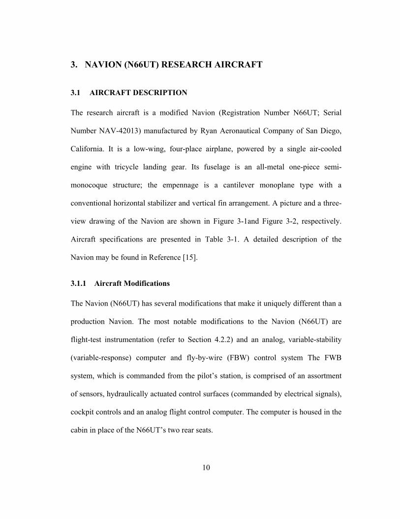
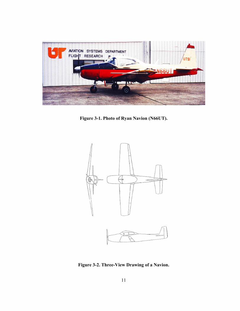
conventional horizontal stabilizer and vertical fin arrangement. A picture and a three-
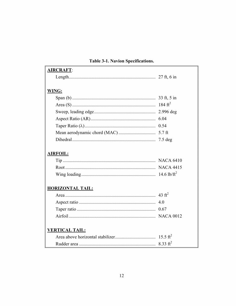
view drawing of the Navion are shown in Figure 3-1and Figure 3-2, respectively.
Aircraft specifications are presented in Table 3-1. A detailed description of the
Navion may be found in Reference [15].
3.1.1 Aircraft Modifications
The Navion (N66UT) has several modifications that make it uniquely different than a
production Navion. The most notable modifications to the Navion (N66UT) are
flight-test instrumentation (refer to Section 4.2.2) and an analog, variable-stability
(variable-response) computer and fly-by-wire (FBW) control system The FWB
system, which is commanded from the pilot’s station, is comprised of an assortment
of sensors, hydraulically actuated control surfaces (commanded by electrical signals),
cockpit controls and an analog flight control computer. The computer is housed in the
cabin in place of the N66UT’s two rear seats.
11
Figure 3-1. Photo of Ryan Navion (N66UT).
Figure 3-2. Three-View Drawing of a Navion.
12
Table 3-1. Navion Specifications.
AIRCRAFT: Length........................................................................... 27 ft, 6 in WING: Span (b) ........................................................................ 33 ft, 5 in Area (S) ........................................................................ 184 ft2 Sweep, leading edge..................................................... 2.996 deg Aspect Ratio (AR)........................................................ 6.04 Taper Ratio (λ) ............................................................. 0.54 Mean aerodynamic chord (MAC) ................................ 5.7 ft Dihedral........................................................................ 7.5 deg AIRFOIL: Tip ................................................................................ NACA 6410 Root .............................................................................. NACA 4415 Wing loading ................................................................ 14.6 lb/ft2 HORIZONTAL TAIL: Area .............................................................................. 43 ft2 Aspect ratio .................................................................. 4.0 Taper ratio .................................................................... 0.67 Airfoil ........................................................................... NACA 0012 VERTICAL TAIL: Area above horizontal stabilizer................................... 15.5 ft2 Rudder area .................................................................. 8.33 ft2
13
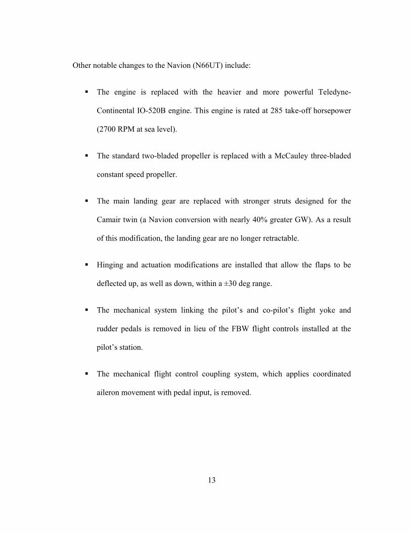
Other notable changes to the Navion (N66UT) include:
� The engine is replaced with the heavier and more powerful Teledyne-
Continental IO-520B engine. This engine is rated at 285 take-off horsepower
(2700 RPM at sea level).
� The standard two-bladed propeller is replaced with a McCauley three-bladed
constant speed propeller.
� The main landing gear are replaced with stronger struts designed for the
Camair twin (a Navion conversion with nearly 40% greater GW). As a result
of this modification, the landing gear are no longer retractable.
� Hinging and actuation modifications are installed that allow the flaps to be
deflected up, as well as down, within a ±30 deg range.
� The mechanical system linking the pilot’s and co-pilot’s flight yoke and
rudder pedals is removed in lieu of the FBW flight controls installed at the
pilot’s station.
� The mechanical flight control coupling system, which applies coordinated
aileron movement with pedal input, is removed.
14
3.2 CONTROL SYSTEM
3.2.1 Cockpit Controls
The conventional flight control system is commanded from the copilot’s station, and
is fully reversible with the FBW system disengaged. The primary cockpit controls
consist of pedals governing rudder action, a control wheel/yoke governing aileron and
elevator action and an engine throttle. As stated previously, the standard rudder-to-
aileron mechanical coupling system, which applies coordinating aileron movement
with pedal input, is removed from the Navion (N66UT).
3.2.2 Moment Controls
Piloted control of the aircraft’s pitching, rolling, and yawing are through conventional
elevator, aileron, and rudder control surfaces, respectively. Additional control of the
aircraft’s pitching is through trim tabs, installed in the trailing edge of each elevator.
The control surfaces are connected to their respective cockpit controls by various
combinations of rods/linkages, bell cranks, cables and pulleys.
3.2.3 Normal Force Control
Control of the aircraft’s normal acceleration is exercised through set of in-board flaps.
As stated previously, the installed flaps have hinging and actuation modifications that
allow the flaps to be deflected over a ±30 deg range. Actuation is hydraulic, with a
maximum available surface rate of 110 deg/sec.
15
4. FLIGHT TEST AND DATA AQUISITION
4.1 FLIGHT TEST
A test flight was conducted on October 9, 1998 to collect short-term frequency
response data of the Navion (N66UT), unaugmented (i.e., with the FBW system
disengaged). The essential test elements were on-axis pilot-generated-frequency-
sweep inputs for each control axis (directional, lateral, longitudinal, and thrust). In
total, data was collected for 12 frequency sweeps; three on-axis frequency sweeps
were conducted for each control axis. The flight crew consisted of two crewmembers,
an experimental test pilot and a flight test engineer. The test pilot flew all
experimental maneuvers. The flight test engineer manually activated the data
recording process, monitored the data on strip charts and provided timing cues to the
test pilot. The duration of the test flight was 1.5 hours.
4.1.1 Flight Test Conditions
The test flight was conducted in calm air under daylight visual meteorological
conditions (VMC) at the Tullahoma Municipal Airport, Tullahoma, Tennessee, on
October 9, 1998. The test was conducted within the existing envelope of the aircraft
with the canopy closed, flaps at 0°, the landing gear extended, the FBW system
disengaged and with the heater and carburetor heat off. The trim configuration was
steady-state horizontal flight at 90 KCAS at about 5000 ft Hd. The average gross
weight and C.G. for the data collection flight were 3,242 pounds and 100.3 inches aft
16
of datum (24.4% M.A.C.), respectively (refer to Figure A-2 for weight and balance
calculations).
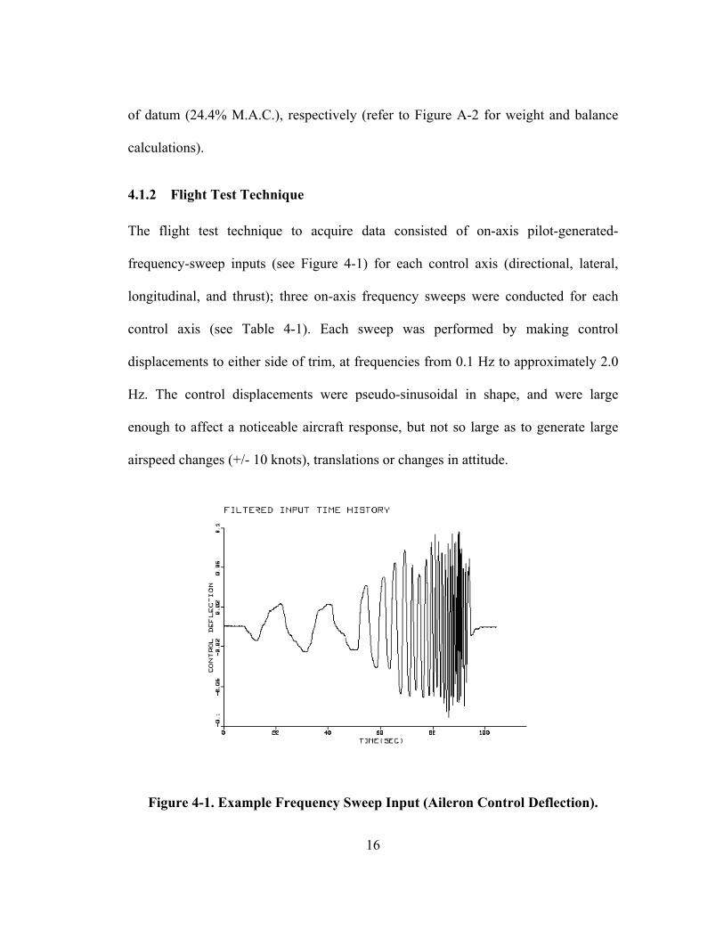
4.1.2 Flight Test Technique
The flight test technique to acquire data consisted of on-axis pilot-generated-
frequency-sweep inputs (see Figure 4-1) for each control axis (directional, lateral,
longitudinal, and thrust); three on-axis frequency sweeps were conducted for each
control axis (see Table 4-1). Each sweep was performed by making control
displacements to either side of trim, at frequencies from 0.1 Hz to approximately 2.0
Hz. The control displacements were pseudo-sinusoidal in shape, and were large
enough to affect a noticeable aircraft response, but not so large as to generate large
airspeed changes (+/- 10 knots), translations or changes in attitude.
Figure 4-1. Example Frequency Sweep Input (Aileron Control Deflection).
17
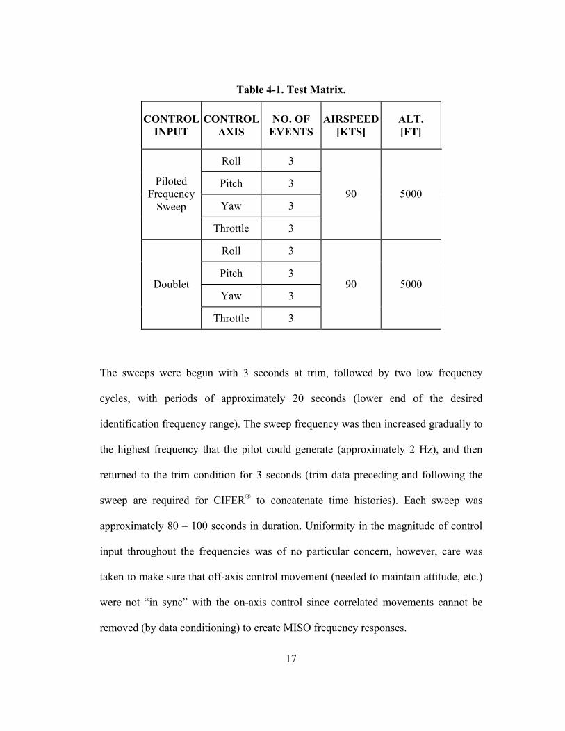
Table 4-1. Test Matrix.
CONTROL INPUT
CONTROL AXIS
NO. OF EVENTS
AIRSPEED[KTS]
ALT. [FT]
Roll 3
Pitch 3
Yaw 3
Piloted Frequency
Sweep
Throttle 3
90 5000
Roll 3
Pitch 3
Yaw 3 Doublet
Throttle 3
90 5000
The sweeps were begun with 3 seconds at trim, followed by two low frequency
cycles, with periods of approximately 20 seconds (lower end of the desired
identification frequency range). The sweep frequency was then increased gradually to
the highest frequency that the pilot could generate (approximately 2 Hz), and then
returned to the trim condition for 3 seconds (trim data preceding and following the
sweep are required for CIFER® to concatenate time histories). Each sweep was
approximately 80 – 100 seconds in duration. Uniformity in the magnitude of control
input throughout the frequencies was of no particular concern, however, care was
taken to make sure that off-axis control movement (needed to maintain attitude, etc.)
were not “in sync” with the on-axis control since correlated movements cannot be
removed (by data conditioning) to create MISO frequency responses.
18
Control doublets, at various frequencies and amplitudes, for each control axis were
performed in addition to the frequency sweeps. The data from the doublets are needed
for time-domain verification of the identification results.
4.1.3 Special Flight Test Precautions
There is a high potential for structural damage during ‘bandwidth’ testing, not
excluding damage severe enough to led to the total loss of the aircraft. More
specifically, there is the possibility of accidentally exciting a vibratory mode at or
near the natural frequency of a structural member or other aircraft component,
particularly if inputs are made with higher magnitudes or frequencies than required.
Because the test aircraft was not instrumented for continuous measurement of real
time structural loads, precautions were taken to start frequency sweeps with small
magnitude inputs at low frequency, increase the magnitude of inputs through the
middle frequency range and decrease the magnitude of the inputs at high frequency.
Additionally, the aircraft’s input and response parameters were monitored to observe
any abnormalities/inconstancies in the data that would suggest a hazardous flight
situation.
4.2 DATA AQUISITION
4.2.1 Cockpit Instrumentation
Air data (airspeed and altitude) and engine parameters (manifold pressure and RPM),
as well as OAT, were recorded by hand on flight data cards referencing the aircrafts
cockpit instrumentation.
19
4.2.2 Flight Test Instrumentation
Potentiometers, gyroscopes, and linear accelerometers were used in conjunction with
a data acquisition system (refer to Section 4.2) to record the input and output
parameters presented in Table 4-2. Five (5) potentiometers were used to measure
surface positions and body attitudes; the potentiometers were located at their
respective control surfaces. Three (3) gyroscopes were used to measure body rates;
the gyros were located in the rear of the cabin “near” the C.G.. Three (3)
accelerometers were used to measure body accelerations. The accelerometers were
mounted together 2.3 inches forward of the aircraft’s longitudinal C.G. or 98 inches
aft of datum (see Figure A-2). The placement of the accelerometer package relative to
the aircraft’s vertical C.G. was “backed out” during the model identification process
using basic kinematic relationships. The package was estimated to be about 2.4 inches
(0.1977 ft) below the vertical C.G.
4.2.3 Data Acquisition System
A personal computer-based data acquisition system was used for the test flights. The
system was comprised of a 12-bit, multi-plexed analog-to-digital (A/D) converter (a
IoTech DaqBook® 120 shown in Figure A-3) and a 120 Mhz Pentium® notebook
computer. Using IoTech’s DaqView® software, the computer served three functions:
(1) to control the DaqBook; (2) to provide real-time storage of all the measured input
and output parameters (see Table 3-1) for post acquisition retrieval; and (3) to display
real-time strip charts of each input channel.
20
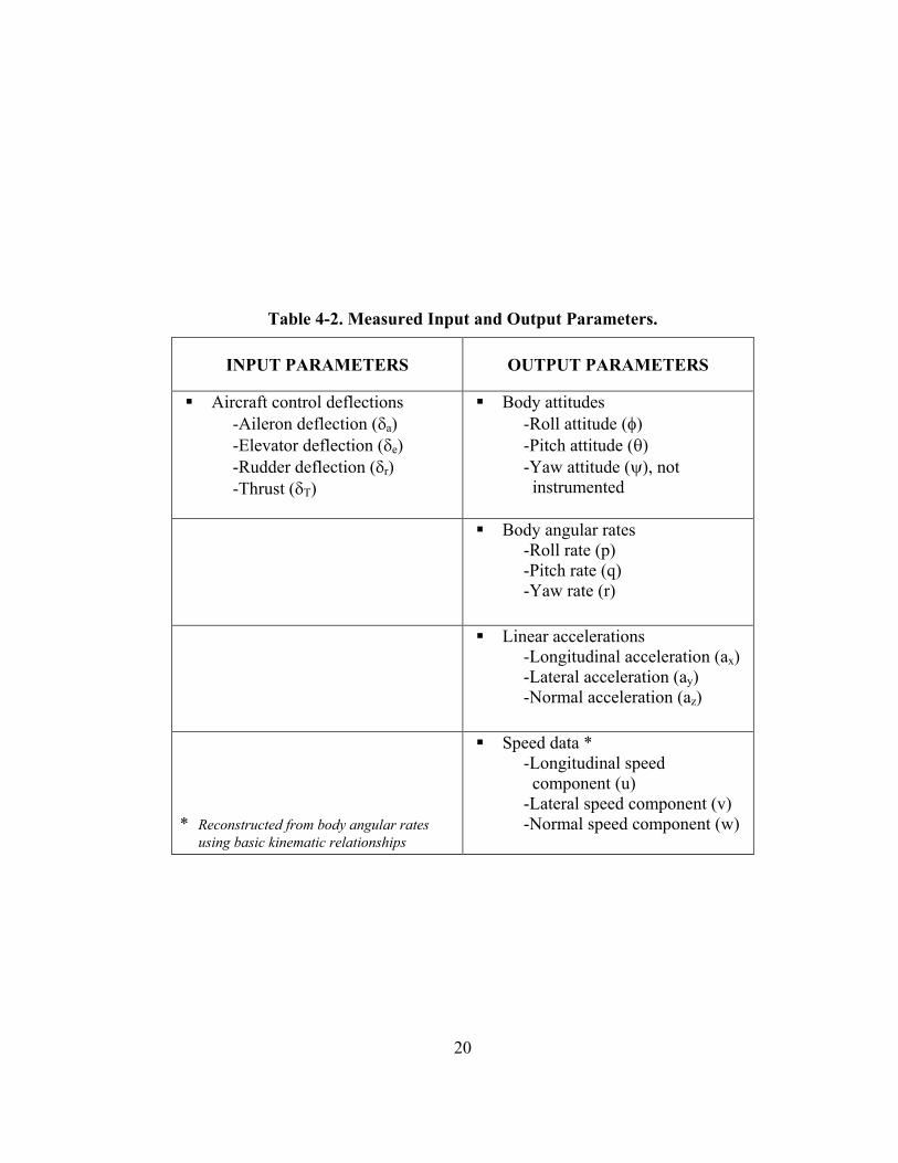
Table 4-2. Measured Input and Output Parameters.
INPUT PARAMETERS OUTPUT PARAMETERS
� Aircraft control deflections -Aileron deflection (δa) -Elevator deflection (δe) -Rudder deflection (δr) -Thrust (δT)
� Body attitudes -Roll attitude (φ) -Pitch attitude (θ) -Yaw attitude (ψ), not instrumented
� Body angular rates -Roll rate (p) -Pitch rate (q) -Yaw rate (r)
� Linear accelerations -Longitudinal acceleration (ax) -Lateral acceleration (ay) -Normal acceleration (az)
* Reconstructed from body angular rates
using basic kinematic relationships
� Speed data * -Longitudinal speed component (u) -Lateral speed component (v) -Normal speed component (w)
21
The system was setup to measure voltage differential across 16 single-ended, bipolar
input channels (see Table A-1). Total data transfer rates for the test were on the order
of 800 Kbytes/sec at a sampling rate of 100 Hz for all channels—channel sequencing
was at 10 millisecond intervals.
A sufficient number of anti-aliasing filters (one for each channel) were not available;
thus, filters were not used so as not to induce phase shifts in the data of specific
channels, or otherwise condition specific data in anyway. It should be noted,
however, that “pre-filtering” of the data is typically done to remove high frequency
“noise”, such as structural and engine vibrations. High frequency content, outside the
range of interest, was digitally filtered out during data conditioning (refer to Section
5.1).
22
5. PARAMETER IDENTIFICATION AND MODELING
Parameter identification and model structure determination, including all necessary
data conditioning and analysis, for this study were accomplished using CIFER® 3.0
(Comprehensive Identification from FrEquency Responses), a system identification
and verification software facility developed by Mark Tischler and Mavis Cauffman of
the U.S. Army’s Aeroflightdynamics Directorate (AFDD) and Mavis Cauffman of
Sterling Software, Inc, respectively. The identification process followed for this study
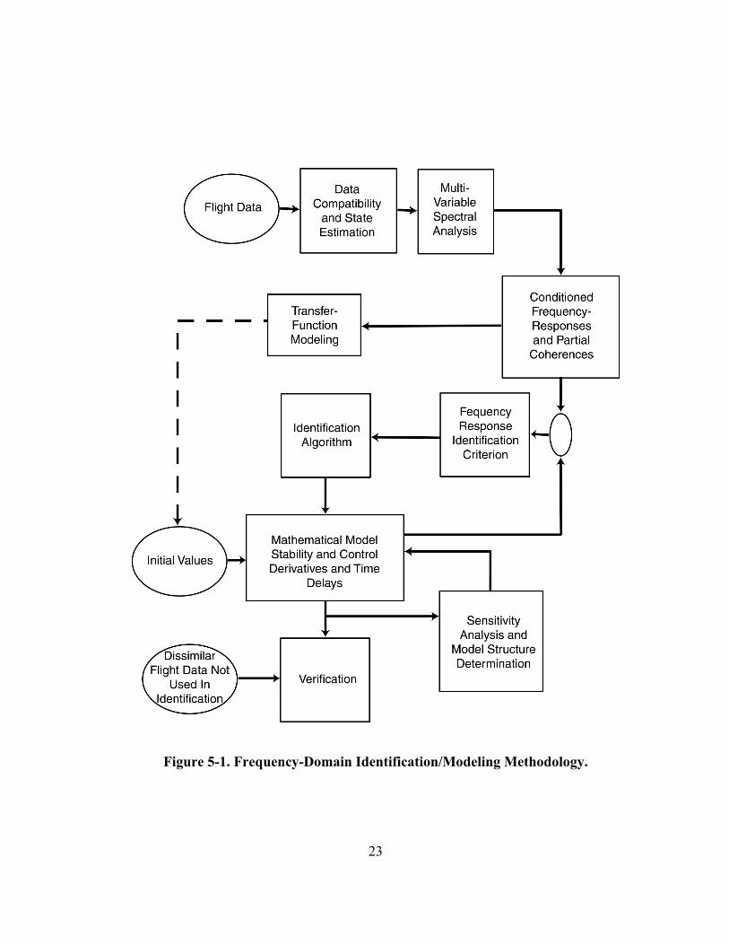
is presented in Figure 5-1. A detailed description of the identification methodology,
as well as the specific capabilities of CIFER®, may be found in Reference [14].
5.1 DATA CONDITIONING AND COMPATABILITY
The starting point for frequency-domain identification is data conditioning. Unlike
time-domain approaches, frequency-domain analysis requires that the time-based data
be converted to frequency-based data used to create frequency responses of each
input/output pair. The extraction of frequency data from the parameter time histories
is achieved with CIFER® using the Chirp-Z or “Zoom” FFT. It should be noted that
the data is also typically pre-processed for dropouts using a “smoother” (e.g., Kalman
filtering) to avoid computational problems. However, the capability to “smooth” the
data was not available for this study—no computational problems were encountered
during the subsequent analysis. Also, the time history data for each parameter were
first converted to consistent engineering units and digitally filtered at
23
Figure 5-1. Frequency-Domain Identification/Modeling Methodology.
24
5 Hz to remove high frequency data (noise). The time history sets were additionally
conditioned by digitally resampling the data at 50 Hz—this was done to reduce the
overall computational burden.
5.2 SPECTRAL ANALSIS
The foundation of frequency-domain parameter identification is the creation of
frequency responses using the responses for each input/output [parameter] pair. Three
steps are performed to create the conditioned frequency-responses used for model
structure determination, and ultimately the estimation of the model coefficients (in
this case the stability and control derivatives). The first step is to generate single-
input/single-output (SISO) frequency-responses for each input/output pair for all of
time history records for each “sweep” axis. Of the three (3) sweep data sets collected
for each axis, the “best” two (2) records were selected based on a qualitative
assessment of the spectral functions for select frequency response pairs. The two (2)
time history records were then concatenated to form a single record. SISO frequency
responses were then created for the concatenated records. Also included in the
analysis are frequency responses for pseudo measurements of udot, vdot, and wdot
(used for model identification). These pseudo states are reconstructed from the
[measured] inputs/outputs using the basic kinematic relationships presented in
Equation 8. Next, “poor” quality frequency-responses, as well as responses that
showed no correlation, are removed based on analysis of the spectral functions
(coherence, cross-spectrum, input-autospectrum, and output-autospectrum) for each
frequency-response pair. Finally, the remaining frequency responses are regenerated
25
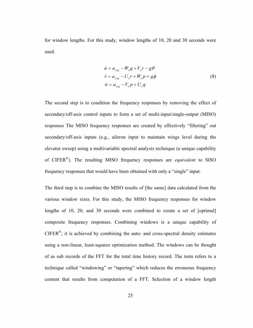
for window lengths. For this study, window lengths of 10, 20 and 30 seconds were
used.
qUpVaw
gpWrUavgrVqWau
oozcg
ooycg
ooxcg
+−=
++−=
−+−=
D
D
D
φ
θ
(8)
The second step is to condition the frequency responses by removing the effect of
secondary/off-axis control inputs to form a set of multi-input/single-output (MISO)
responses The MISO frequency responses are created by effectively “filtering” out
secondary/off-axis inputs (e.g., aileron input to maintain wings level during the
elevator sweep) using a multivariable spectral analysis technique (a unique capability
of CIFER®). The resulting MISO frequency responses are equivalent to SISO
frequency responses that would have been obtained with only a “single” input.
The third step is to combine the MISO results of [the same] data calculated from the
various window sizes. For this study, the MISO frequency responses for window
lengths of 10, 20, and 30 seconds were combined to create a set of [optimal]
composite frequency responses. Combining windows is a unique capability of
CIFER®; it is achieved by combining the auto- and cross-spectral density estimates
using a non-linear, least-squares optimization method. The windows can be thought
of as sub records of the FFT for the total time history record. The term refers to a
technique called “windowing” or “tapering” which reduces the erroneous frequency
content that results from computation of a FFT. Selection of a window length
26
necessarily limits the frequency content of a window (i.e., a sub-record), in that the
lowest frequency possible is that frequency with a corresponding period the size of
the window. Thus, use of a single window is a compromise between having low
frequency content and having a low random error (i.e., erroneous frequency content).
These steps are repeated until composite responses are created for each input/output
pair. An example CIFER® output of the spectral analysis and frequency response
conditioning steps described above is presented in Figure A-4.
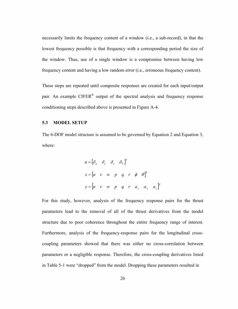
5.3 MODEL SETUP
The 6-DOF model structure is assumed to be governed by Equation 2 and Equation 3,
where:
[ ]TTreau δδδδ=
[ ]Trqpwvux θφ=
[ ]Tzyx aaarqpwvuy =
For this study, however, analysis of the frequency response pairs for the thrust
parameters lead to the removal of all of the thrust derivatives from the model
structure due to poor coherence throughout the entire frequency range of interest.
Furthermore, analysis of the frequency-response pairs for the longitudinal cross-
coupling parameters showed that there was either no cross-correlation between
parameters or a negligible response. Therefore, the cross-coupling derivatives listed
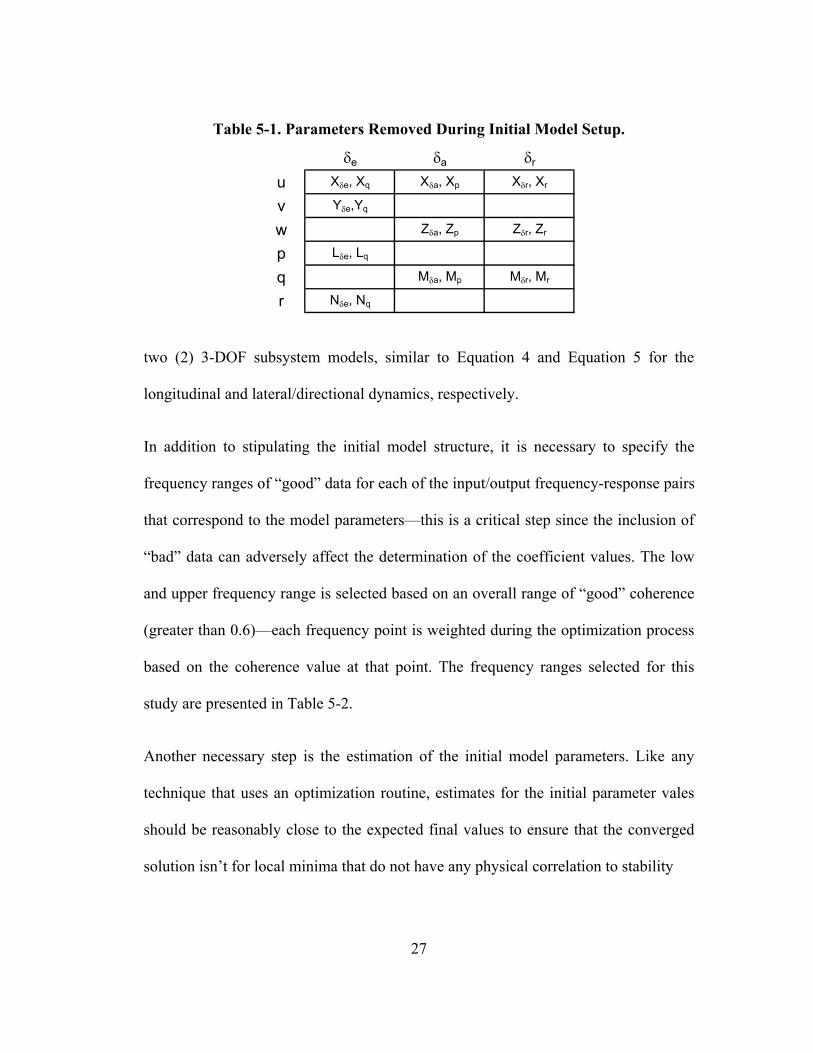
in Table 5-1 were “dropped” from the model. Dropping these parameters resulted in
27
Table 5-1. Parameters Removed During Initial Model Setup.
uvwpqr
Mδr, MrMδa, Mp
δe δa δr
Xδr, Xr
Zδr, Zr
Xδa, Xp
Zδa, Zp
Nδe, Nq
Xδe, Xq
Yδe,Yq
Lδe, Lq
two (2) 3-DOF subsystem models, similar to Equation 4 and Equation 5 for the
longitudinal and lateral/directional dynamics, respectively.
In addition to stipulating the initial model structure, it is necessary to specify the
frequency ranges of “good” data for each of the input/output frequency-response pairs
that correspond to the model parameters—this is a critical step since the inclusion of
“bad” data can adversely affect the determination of the coefficient values. The low
and upper frequency range is selected based on an overall range of “good” coherence
(greater than 0.6)—each frequency point is weighted during the optimization process
based on the coherence value at that point. The frequency ranges selected for this
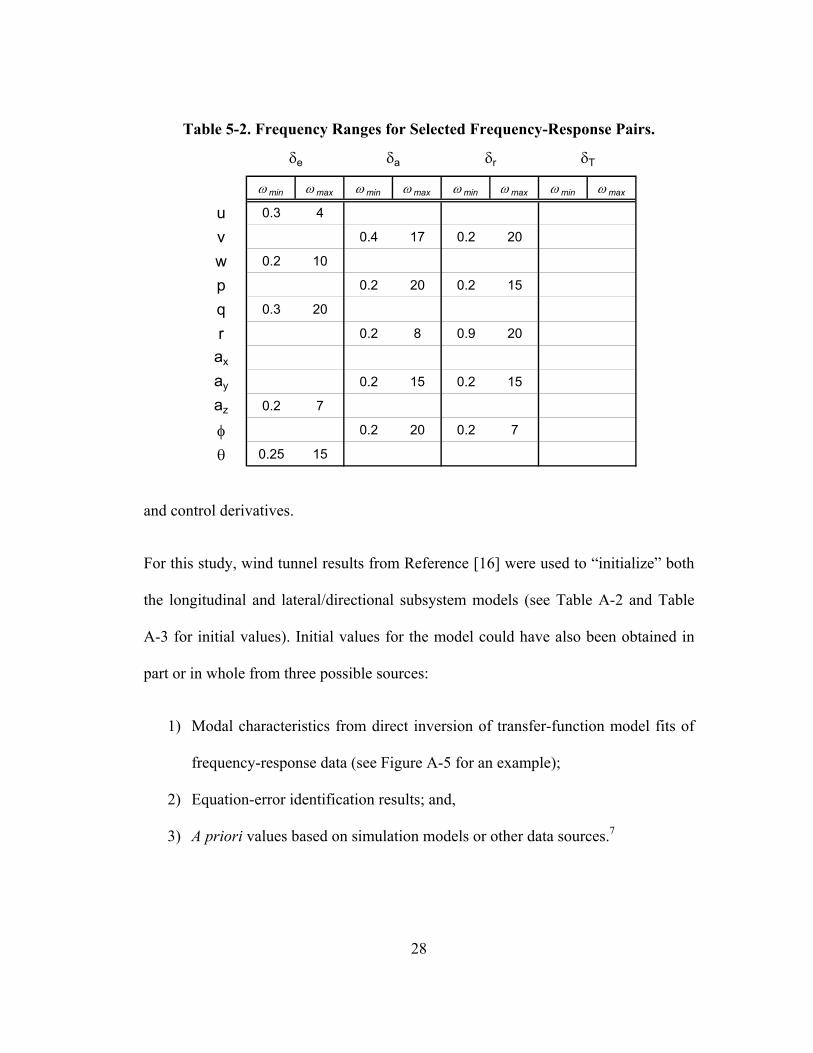
study are presented in Table 5-2.
Another necessary step is the estimation of the initial model parameters. Like any
technique that uses an optimization routine, estimates for the initial parameter vales
should be reasonably close to the expected final values to ensure that the converged
solution isn’t for local minima that do not have any physical correlation to stability
28
Table 5-2. Frequency Ranges for Selected Frequency-Response Pairs.
ω min ω max ω min ω max ω min ω max ω min ω max
u 0.3 4
v 0.4 17 0.2 20
w 0.2 10
p 0.2 20 0.2 15
q 0.3 20
r 0.2 8 0.9 20
ax
ay 0.2 15 0.2 15
az 0.2 7
φ 0.2 20 0.2 7
θ 0.25 15
δe δa δr δT
and control derivatives.
For this study, wind tunnel results from Reference [16] were used to “initialize” both
the longitudinal and lateral/directional subsystem models (see Table A-2 and Table
A-3 for initial values). Initial values for the model could have also been obtained in
part or in whole from three possible sources:
1) Modal characteristics from direct inversion of transfer-function model fits of
frequency-response data (see Figure A-5 for an example);
2) Equation-error identification results; and,
3) A priori values based on simulation models or other data sources.7
29
5.4 MODEL STRUCTURE DETERMINATION
The purpose of model structure determination is to identify and remove parameters
that either do not contribute or only marginally contribute to the fidelity of the model.
Using CIFER®, the state-space models of some specified general structure and of
high-order are simultaneously fitted for all the frequency responses. The process is
iterative; it involves minimizing the weighted square-error between the measured
frequency responses (see Figure A-4) and the model’s frequency responses. The
parameter values are determined with CIFER® using a nonlinear pattern search
(Secant) algorithm that matches MISO frequency-responses. The final model
structure is determined by eliminating parameters one-by-one and reconverging the
solution until the error function (i.e., the “cost”) for the model is reduced to an
acceptable level or begins to increase. Parameters that the model is insensitive to or
that are highly correlated to other parameters are identified by their large individual
“cost.” Parameters that the model is insensitive to are removed first (one-by-one), and
the model is reconverged until the solution has insensitivities less than 10%. Then,
parameters that are highly correlated to another parameters or multiple parameters, as
measured by their Cramer-Rao bounds, are eliminated from the model one-by-one,
and the model is reconverged. The judgment as to which parameter to eliminate is
based on confidence ellipsoids and/or physical principals. A minimally parameterized
model is achieved once all the parameters in the converged solution have Cramer-Rao
bounds less than 20%.
30
The converged longitudinal and lateral/directional model parameters, and associated
Cramer Rao bounds and cost functions, are presented in Table A-2 and Table A-3,
respectively. Bode diagrams and coherence plots for the resulting frequency
responses for the longitudinal and lateral/directional models are presented in Figure
A-6 and Figure A-7, respectively.
5.5 TIME DOMAIN VERIFICATION
The final step in the identification process (see Figure 5-1) is model verification.
Ultimately, this step demonstrates the predictive capability of a model by showing the
aircraft’s dynamic behavior, in both magnitude and phase. Verification is
accomplished with CIFER® by driving the identified state-space model(s) with
dissimilar flight (i.e., data not used during the identification process). For this study
control doublets collected during the flight test are used. The unknown [time-domain]
state equation biases and reference (or zero) shifts are determined by performing a
non-iterative minimization of the weighted least square error between the model and
vehicle responses.
The time history plots for the longitudinal and lateral/directional models are presented
in Section 6.2 and Section 6.3 , respectively.
31
6. RESULTS
6.1 GENERAL
3-DOF models for the decoupled longitudinal and lateral/directional, rigid-body
dynamics of the Navion (N66UT) were extracted from flight data for the cruise flight
condition (V = 90 KCAS). The models were derived using the frequency-domain
identification methodology described in Section 1. The resulting model structure (two
3-DOF subsystem models instead of a 6-DOF) was arrived at “a priori” based on
analysis of the MISO frequency responses of the [measured] parameters. The analysis
showed that there was either no cross-correlation between parameters or a negligible
response for the longitudinal cross-coupling parameters. Similarly, analysis of the
thrust parameters lead to the removal of all thrust derivatives due to poor coherence
throughout the entire frequency range of interest. In total, (17) “conditioned”
frequency response pairs were used to determine the model structure. Bode diagrams
of these frequency response pairs, along with a few selected pairs with “poor”
coherence throughout the frequency range, are presented in Figure A-8, Figure A-9
and Figure A-10. The model parameters, the extracted longitudinal and
lateral/directional derivatives, are presented along with the identified models in the
following sections.
6.2 LONGITUDINAL DYNAMICS
The minimally parameterized model identified for the decoupled longitudinal
dynamics is presented in Equation 9. The validity of the model is demonstrated by
32
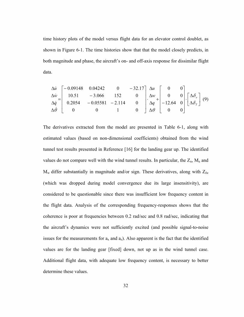
time history plots of the model versus flight data for an elevator control doublet, as
shown in Figure 6-1. The time histories show that that the model closely predicts, in
both magnitude and phase, the aircraft’s on- and off-axis response for dissimilar flight
data.
∆
∆⋅
−+
∆
∆
∆
∆
⋅
−−
−
−−
=
∆
∆
∆
∆
T
e
qwu
qwu
δ
δ
θθ 00064.120000
01000114.205581.02054.00152066.351.10
17.32004242.009148.0
�
�
�
�
(9)
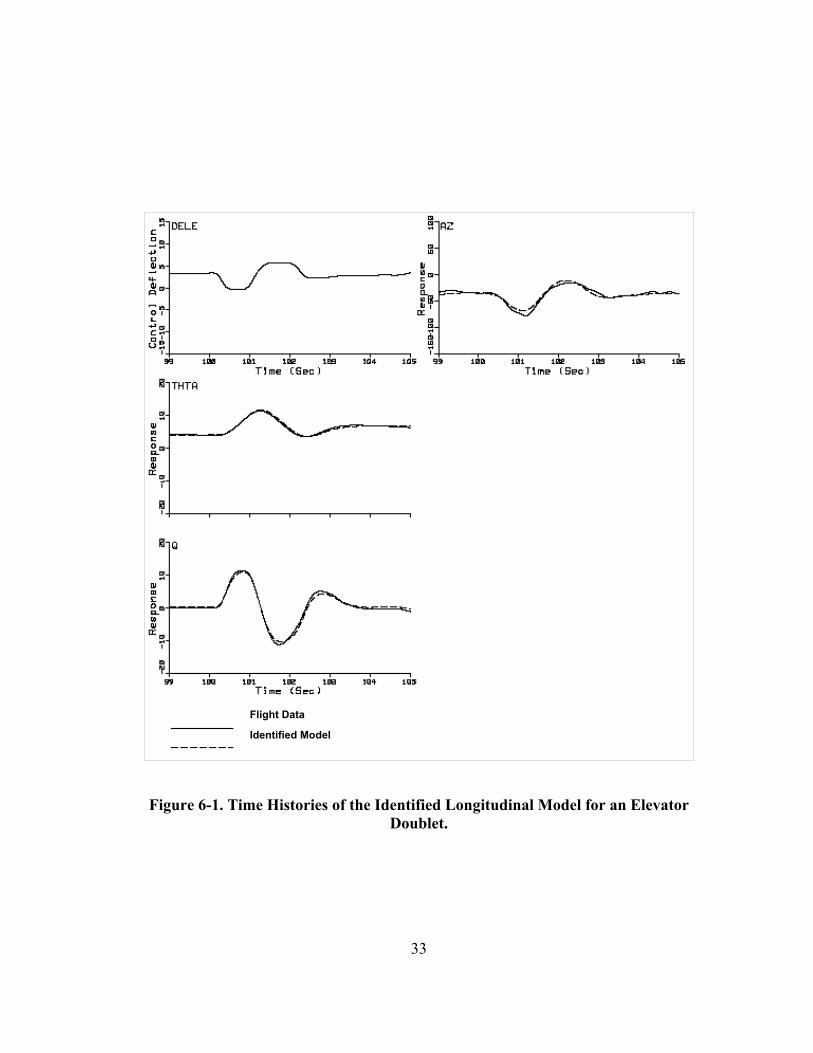
The derivatives extracted from the model are presented in Table 6-1, along with
estimated values (based on non-dimensional coefficients) obtained from the wind
tunnel test results presented in Reference [16] for the landing gear up. The identified
values do not compare well with the wind tunnel results. In particular, the Zu, Mu and
Mw differ substantially in magnitude and/or sign. These derivatives, along with Zδe
(which was dropped during model convergence due its large insensitivity), are
considered to be questionable since there was insufficient low frequency content in
the flight data. Analysis of the corresponding frequency-responses shows that the
coherence is poor at frequencies between 0.2 rad/sec and 0.8 rad/sec, indicating that
the aircraft’s dynamics were not sufficiently excited (and possible signal-to-noise
issues for the measurements for ax and az). Also apparent is the fact that the identified
values are for the landing gear [fixed] down, not up as in the wind tunnel case.
Additional flight data, with adequate low frequency content, is necessary to better
determine these values.
33
Flight Data
Identified Model
Figure 6-1. Time Histories of the Identified Longitudinal Model for an Elevator Doublet.
34
Table 6-1. Identified Longitudinal Dimensional Derivatives.
Name UnitsXu 1/sec -0.092 -0.045
Xw 1/sec 0.0424 0.0361
Zu 1/sec 10.51 -0.37
Zw 1/sec -3.066 -2.024
Zq ft/sec 51.01 --
Mu+MwdotZu 1/(sec ⋅ ft) 0.2054 0.0018
Mw+MwdotZw 1/(sec ⋅ ft) -0.056 -0.039
Mq+Mwdotu o 1/sec -2.114 -2.861
Xδe ft/(sec2) 0 † --
Zδe ft/(sec2) 0 †† -28.17
Mδe+MwdotZδe 1/sec2 -12.67 -11.19
* Body-axis coordinate system† Not included in model structure bases on spectral analysis
†† Eliminated during model structure determination
Derivative * Results from Reference 16
Long
itudi
nal D
eriv
ativ
es
Results from present study
Note: Descriptions of the longitudinal dimensional derivatives can be found in Table A-4.
35
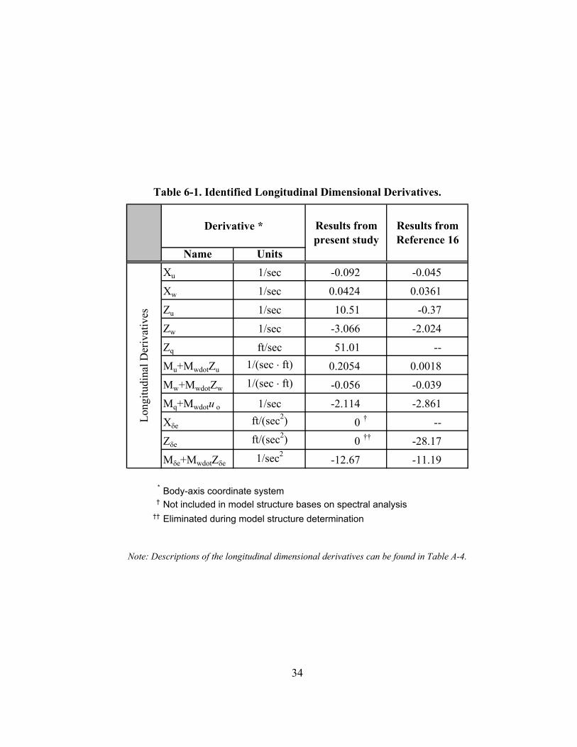
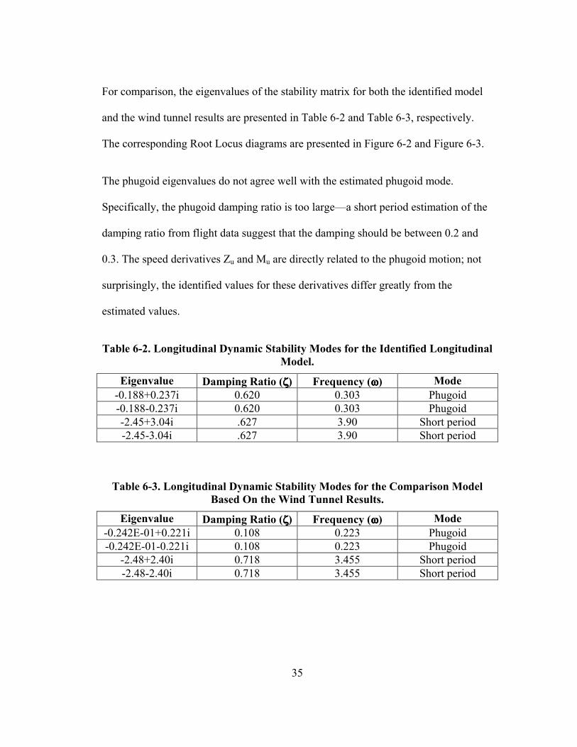
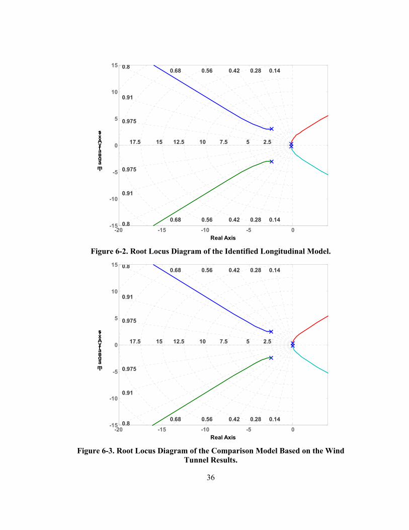
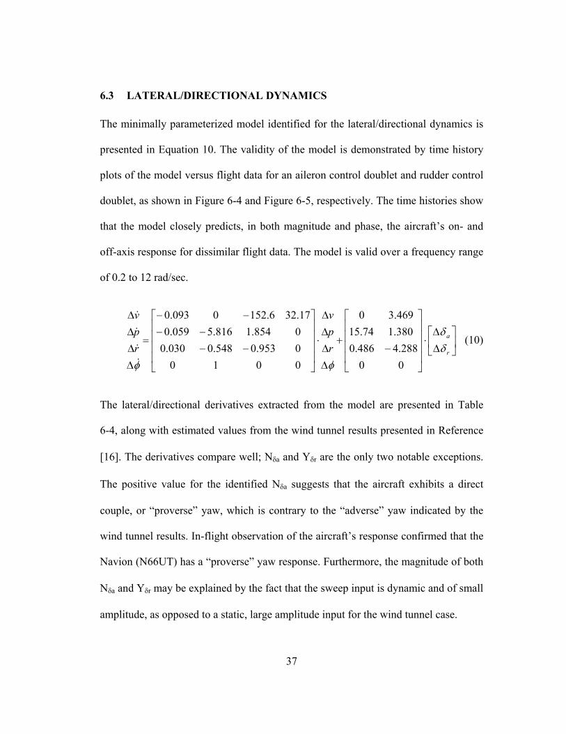
For comparison, the eigenvalues of the stability matrix for both the identified model
and the wind tunnel results are presented in Table 6-2 and Table 6-3, respectively.
The corresponding Root Locus diagrams are presented in Figure 6-2 and Figure 6-3.
The phugoid eigenvalues do not agree well with the estimated phugoid mode.
Specifically, the phugoid damping ratio is too large—a short period estimation of the
damping ratio from flight data suggest that the damping should be between 0.2 and
0.3. The speed derivatives Zu and Mu are directly related to the phugoid motion; not
surprisingly, the identified values for these derivatives differ greatly from the
estimated values.
Table 6-2. Longitudinal Dynamic Stability Modes for the Identified Longitudinal Model.
Eigenvalue Damping Ratio (ζζζζ) Frequency (ωωωω) Mode -0.188+0.237i 0.620 0.303 Phugoid -0.188-0.237i 0.620 0.303 Phugoid -2.45+3.04i .627 3.90 Short period -2.45-3.04i .627 3.90 Short period
Table 6-3. Longitudinal Dynamic Stability Modes for the Comparison Model Based On the Wind Tunnel Results.
Eigenvalue Damping Ratio (ζζζζ) Frequency (ωωωω) Mode -0.242E-01+0.221i 0.108 0.223 Phugoid -0.242E-01-0.221i 0.108 0.223 Phugoid
-2.48+2.40i 0.718 3.455 Short period -2.48-2.40i 0.718 3.455 Short period
36
-20 -15 -10 -5 0-15
-10
-5
0
5
10
15
17.5 15
0.42
0.91
0.68
0.14
12.5
0.68
10 2.57.5
0.8
5
0.975
0.280.56
0.14
0.8
0.28
0.975
0.420.56
0.91
Real Axis
Imaginary Axis
Figure 6-2. Root Locus Diagram of the Identified Longitudinal Model.
-20 -15 -10 -5 0-15
-10
-5
0
5
10
15
17.5 15
0.42
0.91
0.68
0.14
12.5
0.68
10 2.57.5
0.8
5
0.975
0.280.56
0.14
0.8
0.28
0.975
0.420.56
0.91
Real Axis
Imaginary Axis
Figure 6-3. Root Locus Diagram of the Comparison Model Based on the Wind
Tunnel Results.
37
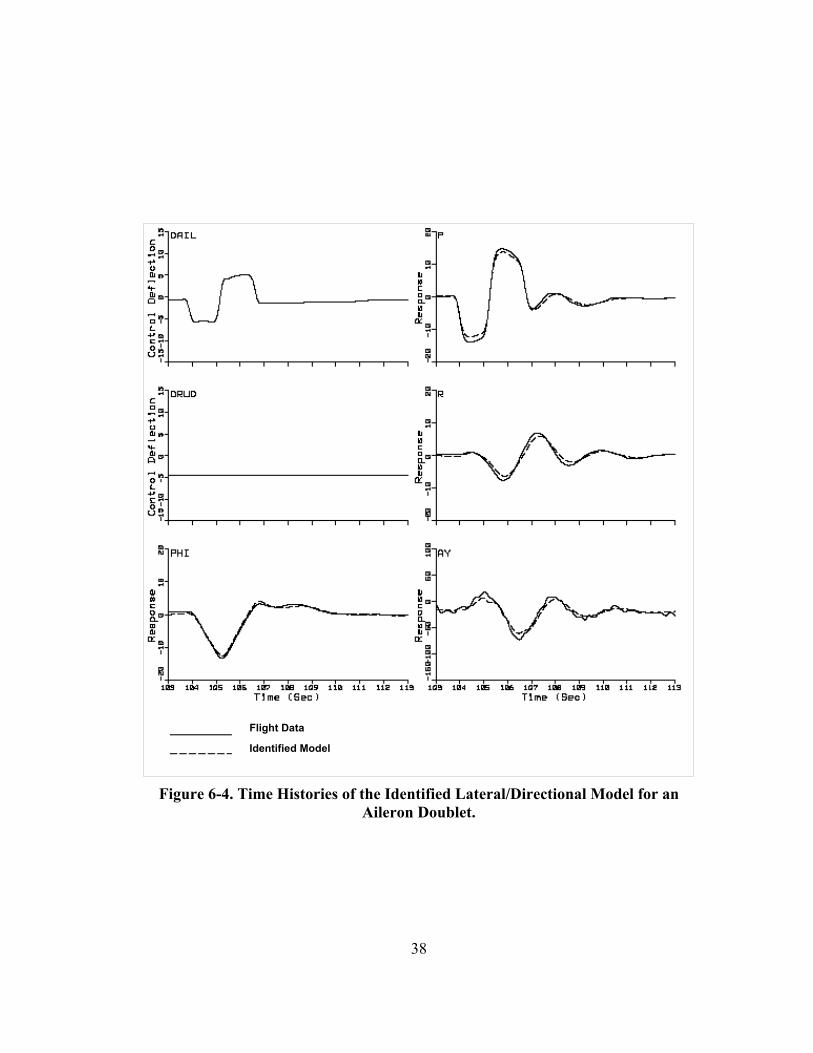
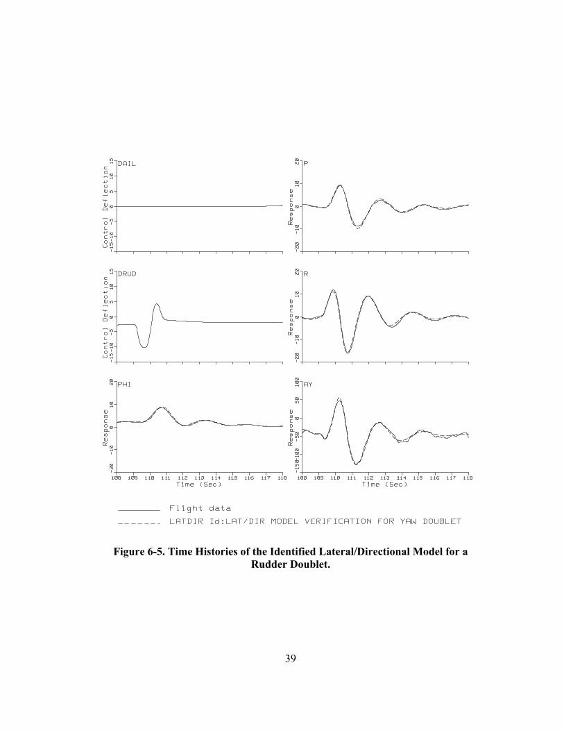
6.3 LATERAL/DIRECTIONAL DYNAMICS
The minimally parameterized model identified for the lateral/directional dynamics is
presented in Equation 10. The validity of the model is demonstrated by time history
plots of the model versus flight data for an aileron control doublet and rudder control
doublet, as shown in Figure 6-4 and Figure 6-5, respectively. The time histories show
that the model closely predicts, in both magnitude and phase, the aircraft’s on- and
off-axis response for dissimilar flight data. The model is valid over a frequency range
of 0.2 to 12 rad/sec.
∆
∆⋅
−+
∆
∆
∆
∆
⋅
−−
−−
−−
=
∆
∆
∆
∆
r
a
rpv
rpv
δ
δ
φφ 00288.4486.0
380.174.15469.30
00100953.0548.0030.00854.1816.5059.017.326.1520093.0
D
D
D
D
(10)
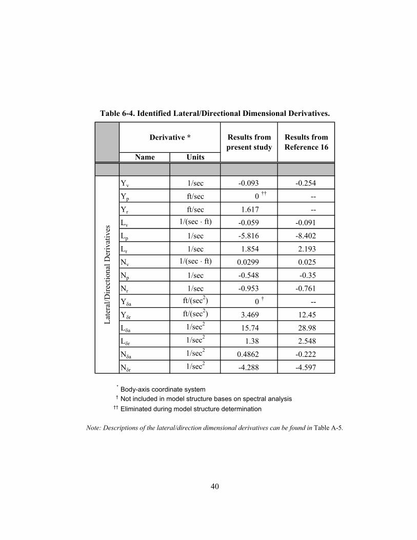
The lateral/directional derivatives extracted from the model are presented in Table
6-4, along with estimated values from the wind tunnel results presented in Reference
[16]. The derivatives compare well; Nδa and Yδr are the only two notable exceptions.
The positive value for the identified Nδa suggests that the aircraft exhibits a direct
couple, or “proverse” yaw, which is contrary to the “adverse” yaw indicated by the
wind tunnel results. In-flight observation of the aircraft’s response confirmed that the
Navion (N66UT) has a “proverse” yaw response. Furthermore, the magnitude of both
Nδa and Yδr may be explained by the fact that the sweep input is dynamic and of small
amplitude, as opposed to a static, large amplitude input for the wind tunnel case.
38
Flight Data
Identified Model
Figure 6-4. Time Histories of the Identified Lateral/Directional Model for an
Aileron Doublet.
39
Figure 6-5. Time Histories of the Identified Lateral/Directional Model for a
Rudder Doublet.
40
Table 6-4. Identified Lateral/Directional Dimensional Derivatives.
Name Units
Yv 1/sec -0.093 -0.254
Yp ft/sec 0 †† --
Yr ft/sec 1.617 --
Lv 1/(sec ⋅ ft) -0.059 -0.091Lp 1/sec -5.816 -8.402
Lr 1/sec 1.854 2.193
Nv 1/(sec ⋅ ft) 0.0299 0.025
Np 1/sec -0.548 -0.35Nr 1/sec -0.953 -0.761
Yδa ft/(sec2) 0 † --
Yδr ft/(sec2) 3.469 12.45
Lδa 1/sec2 15.74 28.98
Lδr 1/sec2 1.38 2.548
Nδa 1/sec2 0.4862 -0.222
Nδr 1/sec2 -4.288 -4.597
* Body-axis coordinate system† Not included in model structure bases on spectral analysis
†† Eliminated during model structure determination
Late
ral/D
irect
iona
l Der
ivat
ives
Derivative * Results from Reference 16
Results from present study
Note: Descriptions of the lateral/direction dimensional derivatives can be found in Table A-5.
41
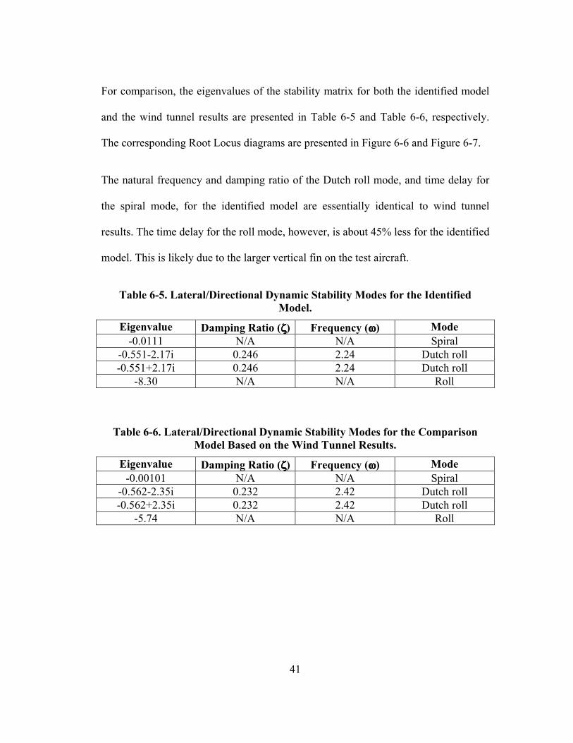
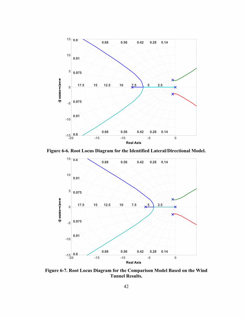
For comparison, the eigenvalues of the stability matrix for both the identified model
and the wind tunnel results are presented in Table 6-5 and Table 6-6, respectively.
The corresponding Root Locus diagrams are presented in Figure 6-6 and Figure 6-7.
The natural frequency and damping ratio of the Dutch roll mode, and time delay for
the spiral mode, for the identified model are essentially identical to wind tunnel
results. The time delay for the roll mode, however, is about 45% less for the identified
model. This is likely due to the larger vertical fin on the test aircraft.
Table 6-5. Lateral/Directional Dynamic Stability Modes for the Identified Model.
Eigenvalue Damping Ratio (ζζζζ) Frequency (ωωωω) Mode -0.0111 N/A N/A Spiral
-0.551-2.17i 0.246 2.24 Dutch roll -0.551+2.17i 0.246 2.24 Dutch roll
-8.30 N/A N/A Roll
Table 6-6. Lateral/Directional Dynamic Stability Modes for the Comparison Model Based on the Wind Tunnel Results.
Eigenvalue Damping Ratio (ζζζζ) Frequency (ωωωω) Mode -0.00101 N/A N/A Spiral
-0.562-2.35i 0.232 2.42 Dutch roll -0.562+2.35i 0.232 2.42 Dutch roll
-5.74 N/A N/A Roll
42
-20 -15 -10 -5 0-15
-10
-5
0
5
10
15
17.5 15
0.42
0.91
0.68
0.14
12.5
0.68
10 2.57.5
0.8
5
0.975
0.280.56
0.14
0.8
0.28
0.975
0.420.56
0.91
Real Axis
Imaginary Axis
Figure 6-6. Root Locus Diagram for the Identified Lateral/Directional Model.
-20 -15 -10 -5 0-15
-10
-5
0
5
10
15
17.5 15
0.42
0.91
0.68
0.14
12.5
0.68
10 2.57.5
0.8
5
0.975
0.280.56
0.14
0.8
0.28
0.975
0.420.56
0.91
Real Axis
Imaginary Axis
Figure 6-7. Root Locus Diagram for the Comparison Model Based on the Wind
Tunnel Results.
43
7. CONCLUDING REMARKS
The identified longitudinal and lateral/directional models closely predict the Navion's
(N66UT) on- and off-axis responses. The extracted lateral/directional derivatives
closely match previous wind tunnel results. The longitudinal derivatives, however,
differ, in some cases significantly, from the previous values. Differences for the
longitudinal derivatives are attributed to insufficient excitation of key parameters
throughout the frequency range of interest, and to differences in the test conditions
(most notably that N66UT has its gear fixed down). Further investigation, including
additional data collection, is required to better identify these derivatives. Such future
efforts should be conducted using a Navion with retractable gear.
44
8. RECOMMENDATIONS
The identification analysis should be re-accomplished for the longitudinal dynamic
model to better characterize Zu, Zδe, Mu and Mw. The additional flight data needed for
this effort should be collected using a Navion with retractable gear so that a more
direct comparison with previous results can be made. The location of the Navion’s
(N66UT) C.G. (vertical, lateral, and longitudinal) should also be determined prior to
collecting any data so that the accelerometers can be [properly] placed at the C.G.—
this will avoid having to “back” out the location, and prevent any unnecessary data
collection errors from being introduced into the analysis.

45
LIST OF REFERENCES
46
WORKS CITED
1) Kimberlin, Ralph, “Parameter Identification Techniques”, Class Notes from a course taught at the University of Tennessee Space Institute, No date.
2) Smetana, F. O., Summey, D. C., and Johnson, W. D., “Flight Testing Techniques for the Evaluation of Light Aircraft Stability Derivatives”, NASA CR2106, May 1972.
3) Eykhoff, Pieter, System Identification, Parameter and State Estimation, John Wiley & Sons, London, 1974.
4) Tischler, Mark B., “Identification and Verification of Frequency-Domain Models for XV-15 Tilt-Rotor Aircraft Dynamics in Cruising Flight”, AIAA Journal of Guidance, Control, and Dynamics, July 1986.
5) Tischler, Mark B., “Frequency-Response Method for Rotorcraft System Identification: Flight Applications to BO-105 Coupled Rotor/Fuselage Dynamics”, Journal of the American Helicopter Society, Vol 37, No 3, pp.. 3-17, July 1992.
6) Tischler, Mark B., “Time and Frequency-Domain Identification and Verification of BO 105 Dynamic Models”, 15th European Rotorcraft Forum, Amsterdam, September 1989.
7) Seckel, E., and Morris, J. J. “The Stability Derivatives of the Navion Aircraft Estimated by Various Methods and Derived From Flight Test Data,” Report No. FAA-RD-71-6, Princeton University, January 1971.
8) Seckel, E. and Morris, J. J., “Full Scale Wind Tunnel Tests of a North American Navion Airframe with Positive and Negative Propeller Thrust and Up and Down Flap Deflection,” Princeton University AMS Report 922, July 1970.
9) R. C. Windgrove, “Estimation of Longitudinal Aircraft Characteristics”, 9th Annual Symposium of the Society of Flight Test Engineers, Arlington, Texas, October 4-6, 1978.
10) Ham, Johnnie A., Tischler, Mark B., “Flight Testing and Frequency Domain Analysis for Rotorcraft Handling Qualities Characteristics”, AHS Specialists’ Meeting on Piloting Vertical Flight Aircraft, 20-23 Jan. 1993, San Francisco, California.
11) Tischler, Mark B., “Identification and Verification of Frequency-Domain Models for XV-15 Tilt-Rotor Aircraft Dynamics in Cruising Flight,” AIAA Journal of Guidance, Control, and Dynamics, July 1986.
WORKS CITED (CONT’D)
47
12) ANON. Technical Memorandum, NASA TM 89422, USAAVSCOM TM 87-A-1, “Demonstration of Frequency-Sweep Testing Technique Using a Bell 214-ST Helicopter”, April 1987.
13) Tischler, Mark B., “Flight Test Manual, Rotorcraft Frequency Domain Flight Testing,” U.S. Army Aviation Technical Test Center, AQTD Project No. 93-14, September 1995.
14) ANON., NASA Conference Publication, NASA CP 10149, USAATCOM TR-94-A-017, "Comprehensive Identification from Frequency Responses", Class Notes from a short course held at NASA Ames Research Center, Moffett Field, California, September 19-23, 1994.
15) ANON., “Navion Service Manual”, First Edition, revised January 1951.
16) Teper, Gary L., “Aircraft Stability and Control Data,” NASA CR-96008, April 1969.
48
WORKS REFERENCED
ANON., Advisory Report, AGARD-AR-280, “Rotorcraft System Identification,” North Atlantic Treaty Organization, September 1991.
ANON., Flight Test Manual, USNTPS-FTM-No. 107, “Rotary Wing Stability and Control,” Patuxent River, Maryland: U.S. Naval Test Pilot School, Naval Air Warfare Center, No Date.
ANON., Military Handbook, MIL-HDBK-1797, “Flying Qualities of Piloted Aircraft”, December 1997.
ANON., Technical Memorandum, NASA TM 110369, USAATCOM TR 95-A-007, “System Identification Methods for Aircraft Flight Control Development and Validation”, October 1995.
ANON., Technical Note, NASA TN D-5857, “Full-Scale Wind-Tunnel Investigation of the Static Longitudinal and Lateral Characteristics of a Light Single-Engine Low-Wing Airplane”, June 1970.ANON., Military Specification, MIL-F-8785C, “Flying Qualities of Piloted Airplanes”, November 1980.
ANON., “The Variable-Response Research Aircraft”, Princeton University, no date.
Basile, P.S., Gripper, S.F., and Kline, G.F., “An Experimental Investigation of the Lateral Dynamic Stability of a Navion Airplane”, Princeton University, June 1970.
Bolding, Randy, “Handling Qualities Evaluation of a Variable Stability Navion Airplane (N66UT) Using Frequency-Domain Test Techniques,” M.S. Thesis, The University of Tennessee Space Institute, December 1998.
Buxo, Arturo Manual, “Performance of the Variable-Stability Navion with Flap Deflection”, MS thesis, The University of Tennessee Space Institute, May 1995.
Catterall, R. Charles, and Lewis, William D., “Determination of Navion Stability and Control Derivatives Using Frequency-Domain Techniques”, American Institute of Aeronautics and Astronautics Conference Publication, AIAA-99-4036, August, 1999.
Cook, M.V., Flight Dynamics Principles, New York, NY: John Wiley & Sons, Inc., 1997.
Fletcher, Jay W., “Obtaining Consistent Models of Helicopter Flight-Data Measurement Errors Using Kinematic-Compatibility and State-Reconstruction
WORKS REFERENCED (CONT’D)
49
Methods”, 46th Annual Forum of the American Helicopter Society, Washington, D.C., May 1990.
Hoh, Roger H., Mitchell, D. G., Ashkenas, I. L., Klein, R. H., Heffley, R. K., and Hodgkinson, J., “Proposed MIL Standard and Handbook-Flying Qualities of Air Vehicles”. AFWAL-TR-82-3081, vol. 2, 1982.
Iliff, K. W., Klein, V., Maine, R. E., and Murray, J., Parameter Estimation Analysis for Aircraft, AIAA Professional Study Series, Williamsburg, VA, 1986.
Kimberlin, Ralph D., “Stability and Control Flight Testing Lecture Notes”, The University of Tennessee Space Institute, No Date.
Lewis, William D., "An Aeroelastic Model Structure Investigation for a Manned Real-Time Rotorcraft Simulation," American Helicopter Society 48th Annual Forum, St. Louis, MO, May 1993.
Nelson, Robert C., Flight Stability and Automatic Control, Second Edition, New York, NY: McGraw-Hill, 1998.
Pierson, Brett M., “Flight Test Safety: Lessons Learned from AN S-3B Flight Test Mishap During a Frequency Domain Test”, M.S. Thesis, The University of Tennessee Space Institute, August 1998.
Tischler, Mark B., “Frequency-Domain Identification of XV-15 Tilt-Rotor Aircraft Dynamics in Hovering Flight”, Paper presented at the AIAA/AHS/IES/SETP/DGLR 2nd Flight Testing Conference, Las Vegas, Nevada, November 1983.
Tischler, Mark B., “Frequency-Response Method for Rotorcraft System Identification: Flight Applications to BO-105 Coupled Rotor/Fuselage Dynamics”, Journal of the American Helicopter Society, Vol 37, No 3, pgs 3-17, July 1992.
Tischler, Mark B., “Flying Quality Analysis and Flight Evaluation of a Highly Augmented Combat Rotorcraft”, Journal of Guidance, Control, and Dynamics, Vol 14, No. 5, pg 954-964, Sep-Oct 1991.
Tischler, Mark B., “Time and Frequency-Domain Identification and Verification of BO 105 Dynamic Models”, 15th European Rotorcraft Forum, Amsterdam, September 1989.

50
APPENDIX
51
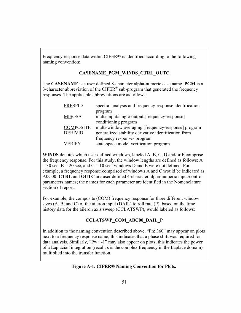
Frequency response data within CIFER® is identified according to the following naming convention:
CASENAME_PGM_WINDS_CTRL_OUTC The CASENAME is a user defined 8-character alpha-numeric case name. PGM is a 3-character abbreviation of the CIFER® sub-program that generated the frequency responses. The applicable abbreviations are as follows:
FRESPID spectral analysis and frequency-response identification program
MISOSA multi-input/single-output [frequency-response] conditioning program
COMPOSITE multi-window averaging [frequency-response] program DERIVID generalized stability derivative identification from
frequency responses program VERIFY state-space model verification program
WINDS denotes which user defined windows, labeled A, B, C, D and/or E comprise the frequency response. For this study, the window lengths are defined as follows: A = 30 sec, B = 20 sec, and C = 10 sec; windows D and E were not defined. For example, a frequency response comprised of windows A and C would be indicated as A0C00. CTRL and OUTC are user defined 4-character alpha-numeric input/control parameters names; the names for each parameter are identified in the Nomenclature section of report. For example, the composite (COM) frequency response for three different window sizes (A, B, and C) of the aileron input (DAIL) to roll rate (P), based on the time history data for the aileron axis sweep (CCLATSWP), would labeled as follows:
CCLATSWP_COM_ABC00_DAIL_P In addition to the naming convention described above, “Ph: 360” may appear on plots next to a frequency response name; this indicates that a phase shift was required for data analysis. Similarly, “Pw: -1” may also appear on plots; this indicates the power of a Laplacian integration (recall, s is the complex frequency in the Laplace domain) multiplied into the transfer function.
Figure A-1. CIFER® Naming Convention for Plots.
52
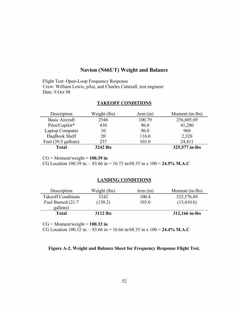
Navion (N66UT) Weight and Balance Flight Test: Open-Loop Frequency Response Crew: William Lewis, pilot, and Charles Catterall, test engineer Date: 9 Oct 98
TAKEOFF CONDITIONS
Description Weight (lbs) Arm (in) Moment (in-lbs)
Basic Aircraft 2546 100.79 256,605.69 Pilot/Copilot* 430 96.0 41,280
Laptop Computer 10 96.0 960 DaqBook Shelf 20 116.0 2,320
Fuel (39.5 gallons) 237 103.0 24,411 Total 3242 lbs 325,577 in-lbs
CG = Moment/weight = 100.39 in CG Location 100.39 in. – 83.66 in = 16.73 in/68.35 in x 100 = 24.5% M.A.C
LANDING CONDITIONS
Description Weight (lbs) Arm (in) Moment (in-lbs) Takeoff Conditions 3242 100.4 325,576.69 Fuel Burned (21.7
gallons) (130.2) 103.0 (13,410.6)
Total 3112 lbs 312,166 in-lbs
CG = Moment/weight = 100.32 in CG Location 100.32 in. – 83.66 in = 16.66 in/68.35 in x 100 = 24.4% M.A.C
Figure A-2. Weight and Balance Sheet for Frequency Response Flight Test.
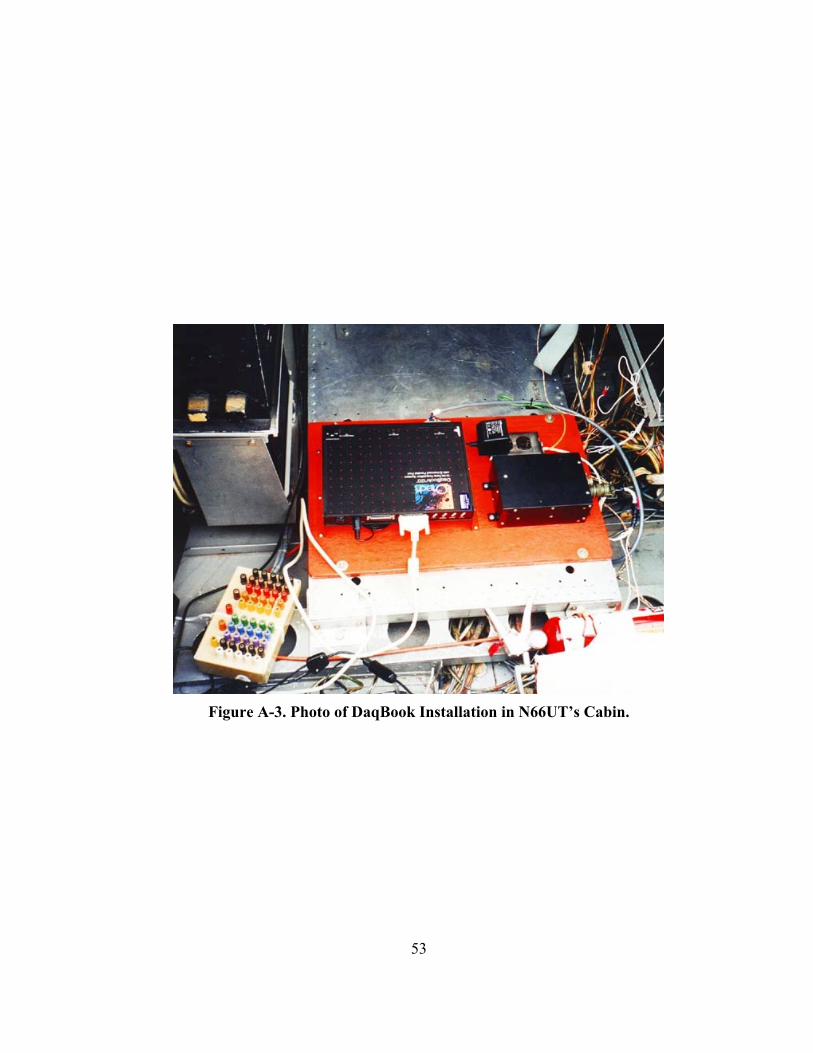
53
Figure A-3. Photo of DaqBook Installation in N66UT’s Cabin.
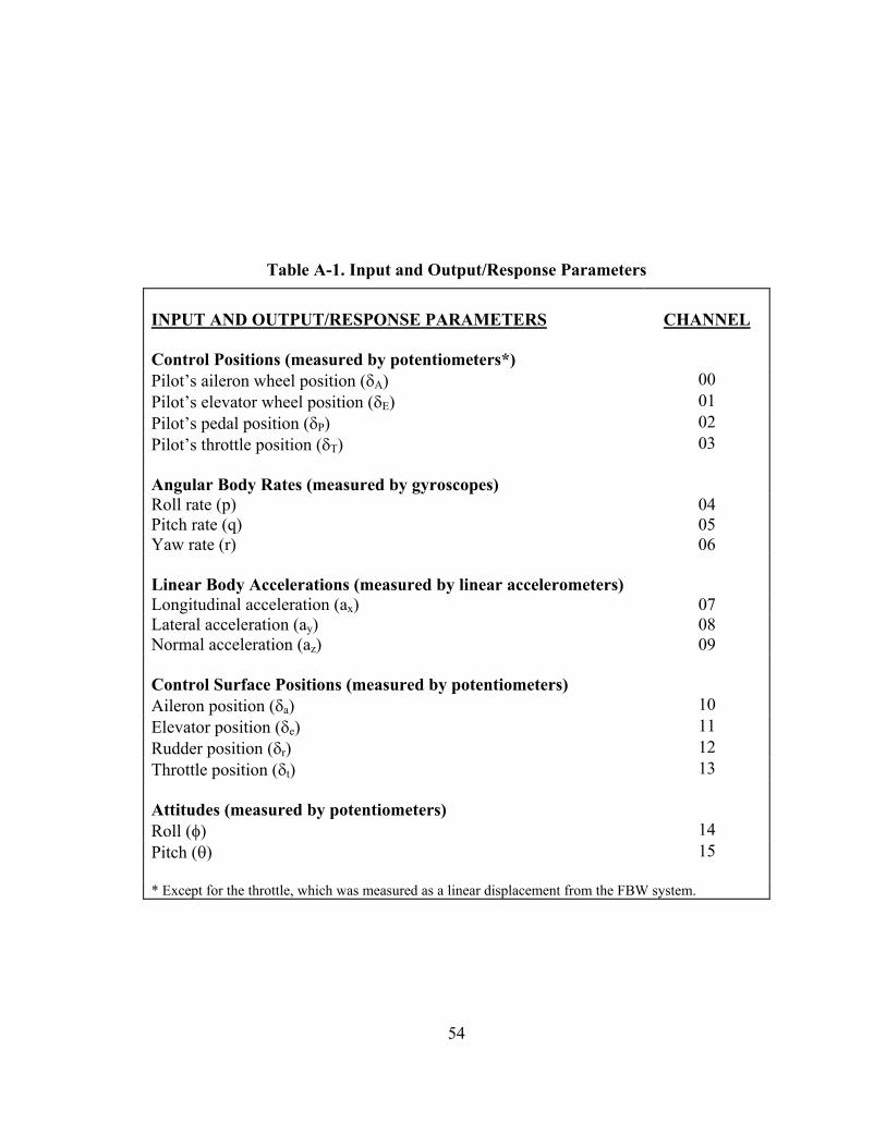
54
Table A-1. Input and Output/Response Parameters
INPUT AND OUTPUT/RESPONSE PARAMETERS
CHANNEL
Control Positions (measured by potentiometers*)
Pilot’s aileron wheel position (δA) 00 Pilot’s elevator wheel position (δE) 01 Pilot’s pedal position (δP) 02 Pilot’s throttle position (δT) 03 Angular Body Rates (measured by gyroscopes)
Roll rate (p) 04 Pitch rate (q) 05 Yaw rate (r) 06 Linear Body Accelerations (measured by linear accelerometers)
Longitudinal acceleration (ax) 07 Lateral acceleration (ay) 08 Normal acceleration (az) 09 Control Surface Positions (measured by potentiometers)
Aileron position (δa) 10 Elevator position (δe) 11 Rudder position (δr) 12 Throttle position (δt) 13 Attitudes (measured by potentiometers)
Roll (φ) 14 Pitch (θ) 15 * Except for the throttle, which was measured as a linear displacement from the FBW system.
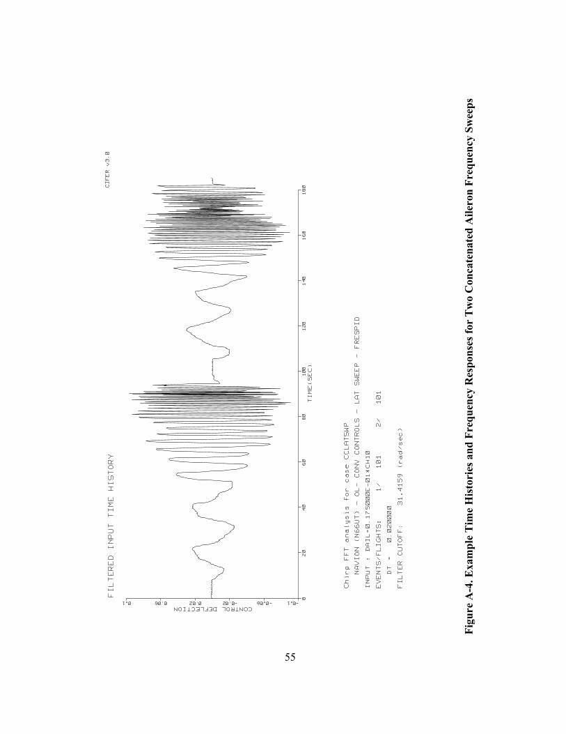
55
Fi
gure
A-4
. Exa
mpl
e T
ime
His
tori
es a
nd F
requ
ency
Res
pons
es fo
r Tw
o C
onca
tena
ted
Aile
ron
Freq
uenc
y Sw
eeps
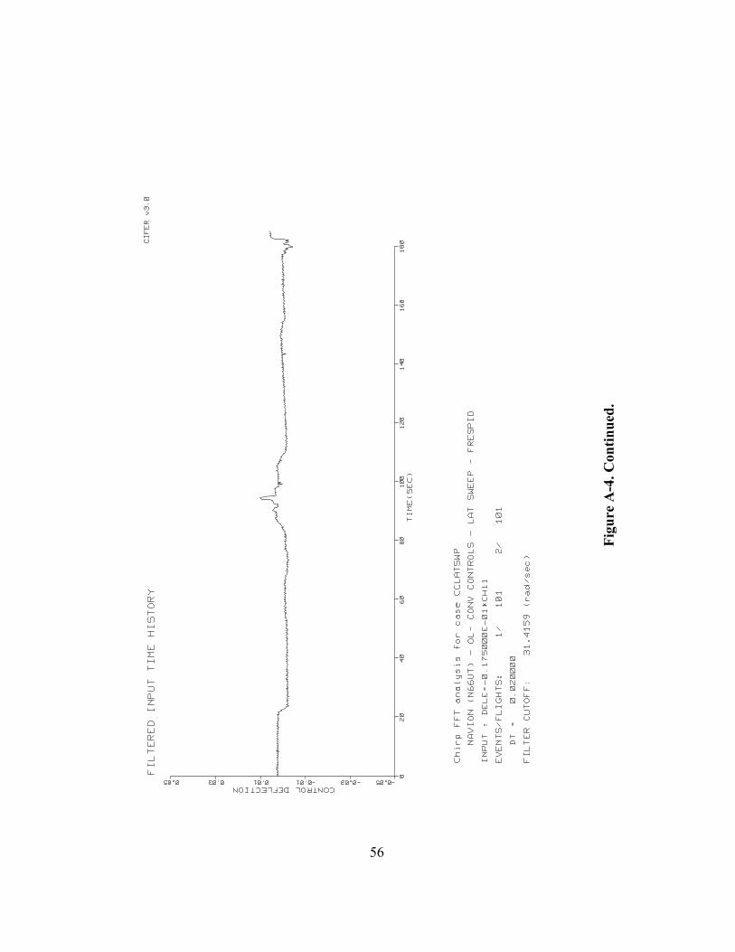
56
Fi
gure
A-4
. Con
tinue
d.

57
Fi
gure
A-4
. Con
tinue
d.
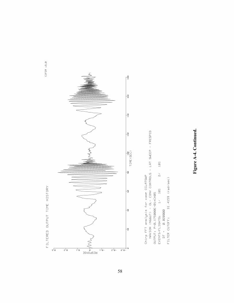
58
Fi
gure
A-4
. Con
tinue
d.
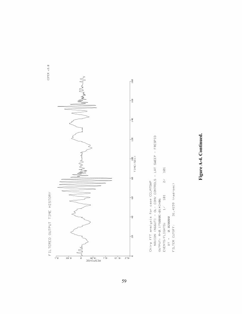
59
Fi
gure
A-4
. Con
tinue
d.
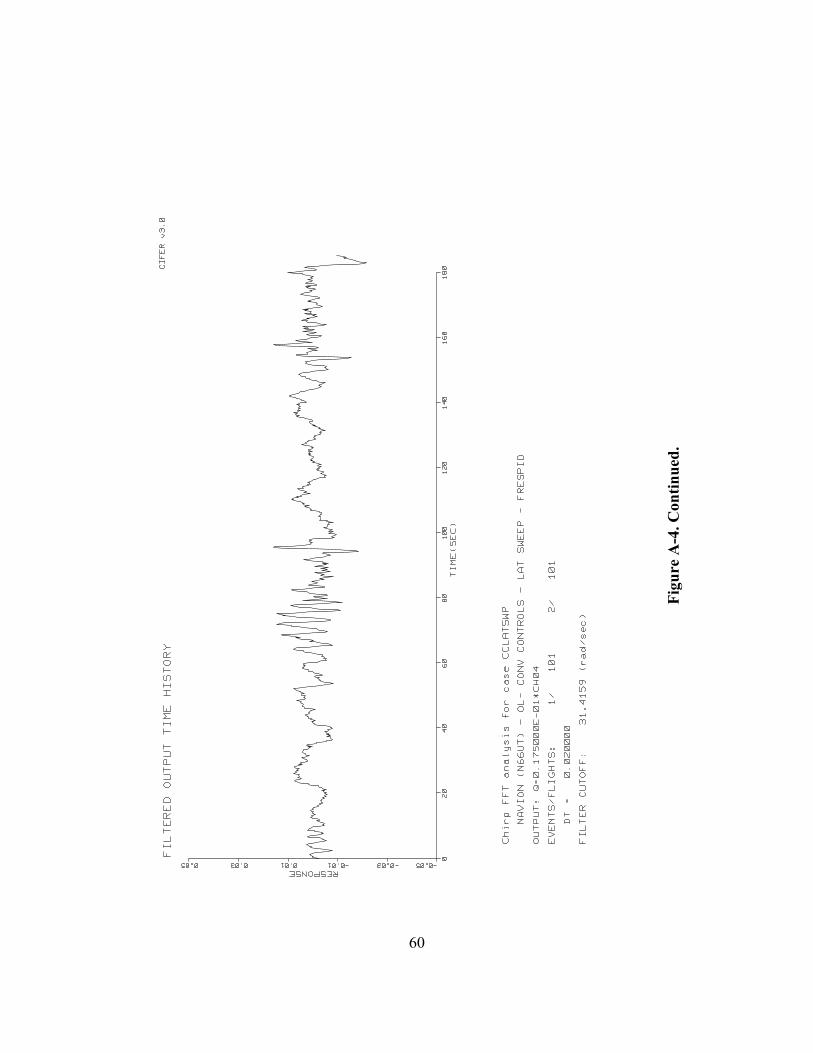
60
Fi
gure
A-4
. Con
tinue
d.
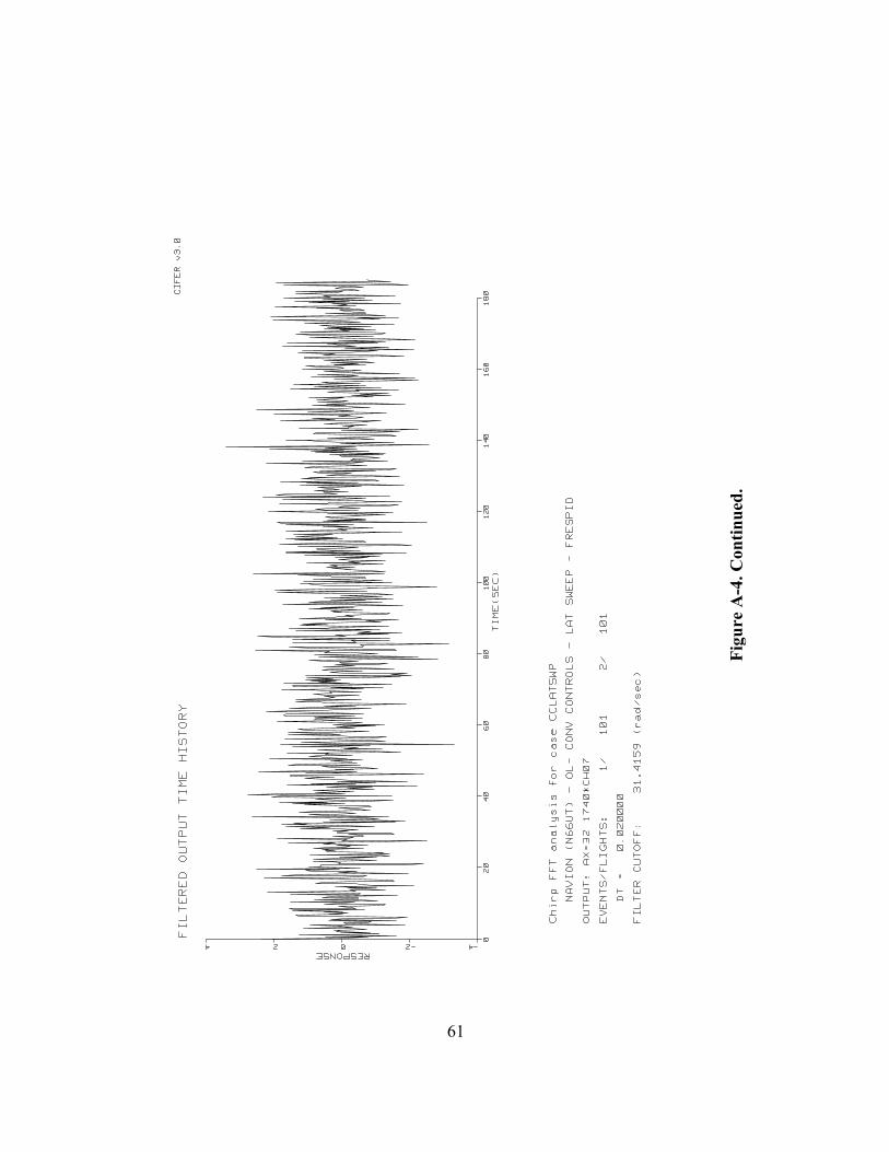
61
Fi
gure
A-4
. Con
tinue
d.
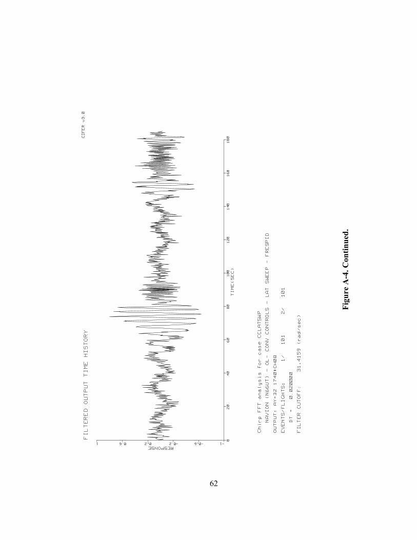
62
Fi
gure
A-4
. Con
tinue
d.
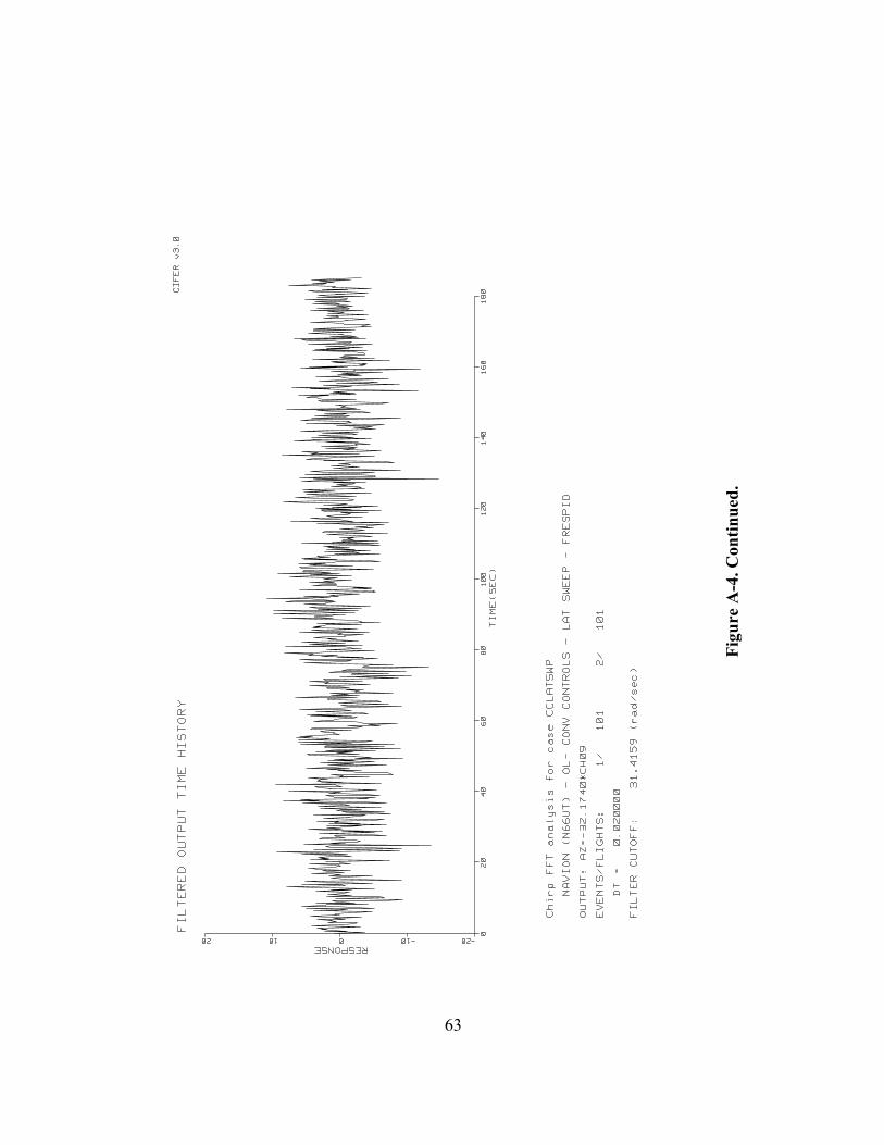
63
Fi
gure
A-4
. Con
tinue
d.
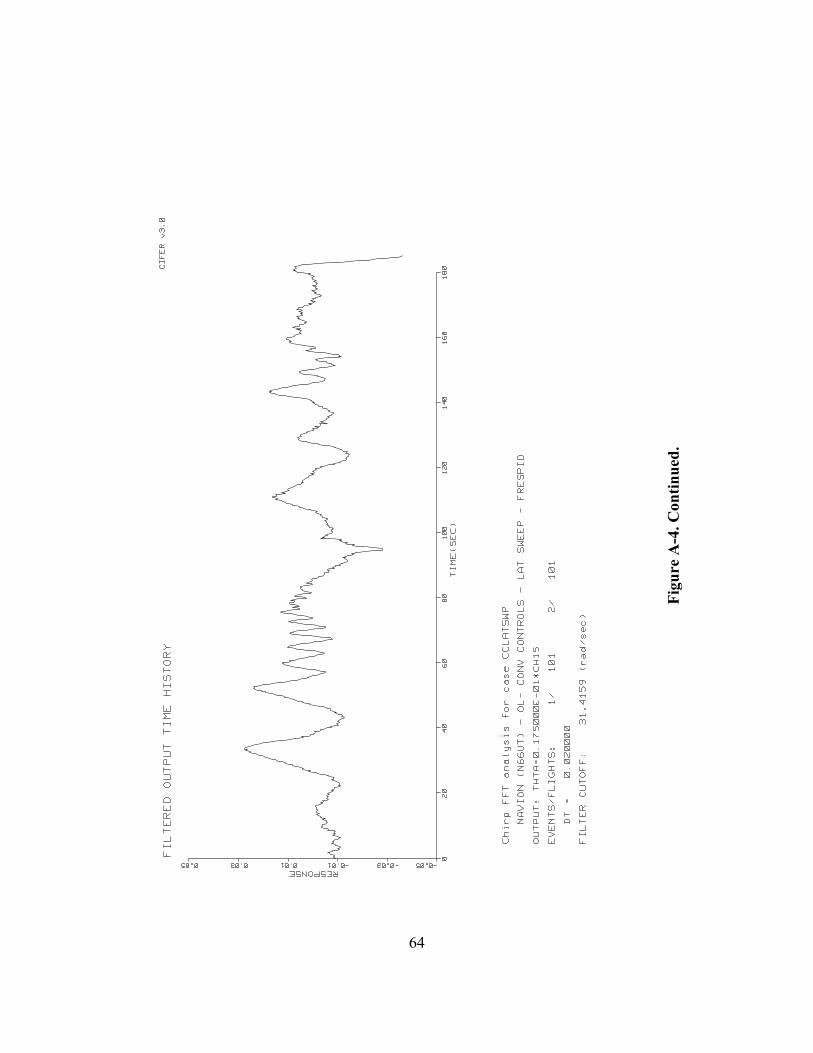
64
Fi
gure
A-4
. Con
tinue
d.
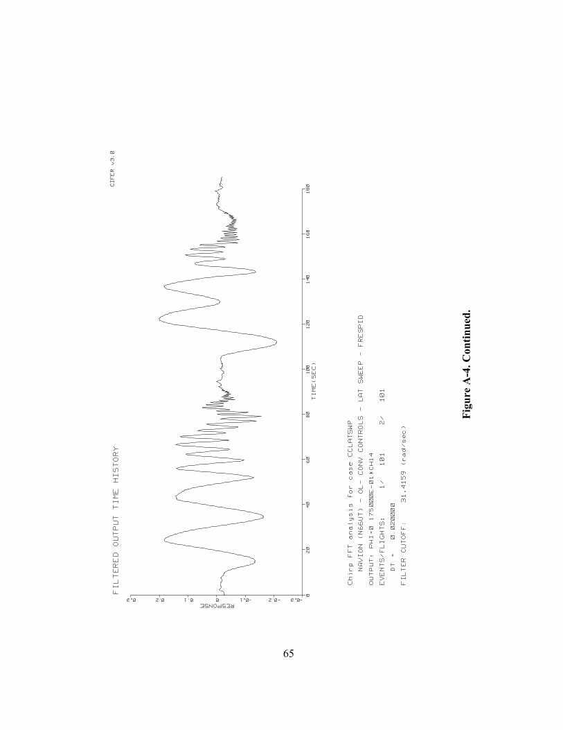
65
Fi
gure
A-4
. Con
tinue
d.
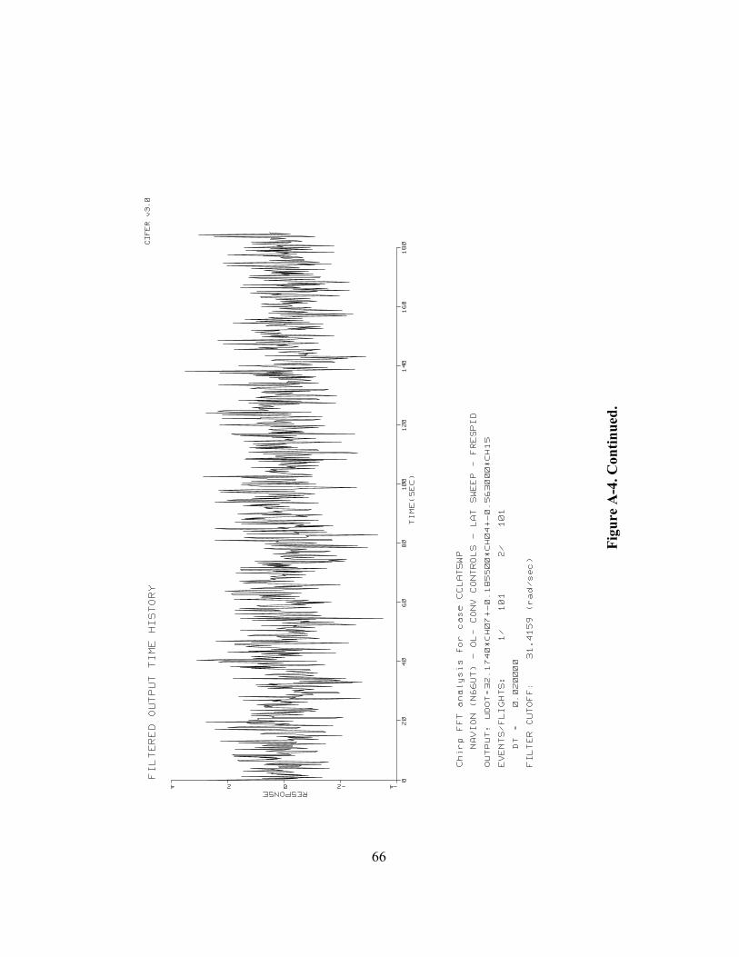
66
Fi
gure
A-4
. Con
tinue
d.
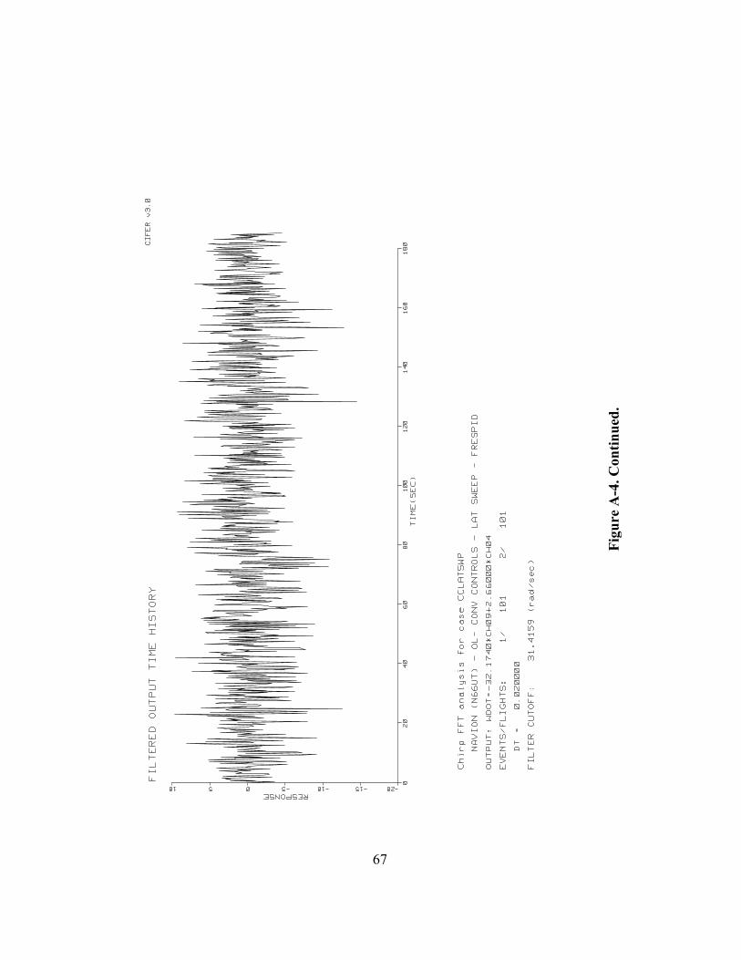
67
Fi
gure
A-4
. Con
tinue
d.
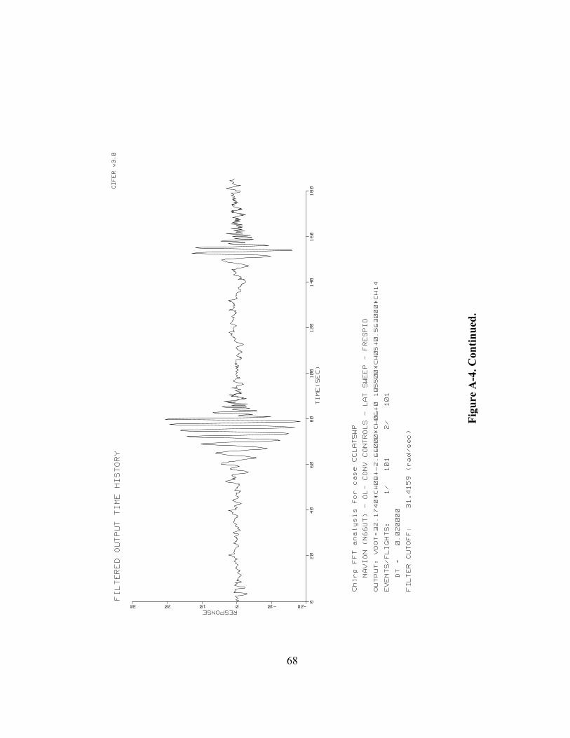
68
Fi
gure
A-4
. Con
tinue
d.
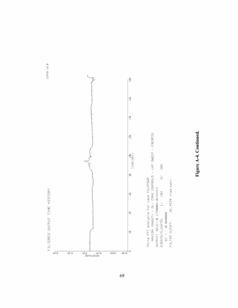
69
Fi
gure
A-4
. Con
tinue
d.
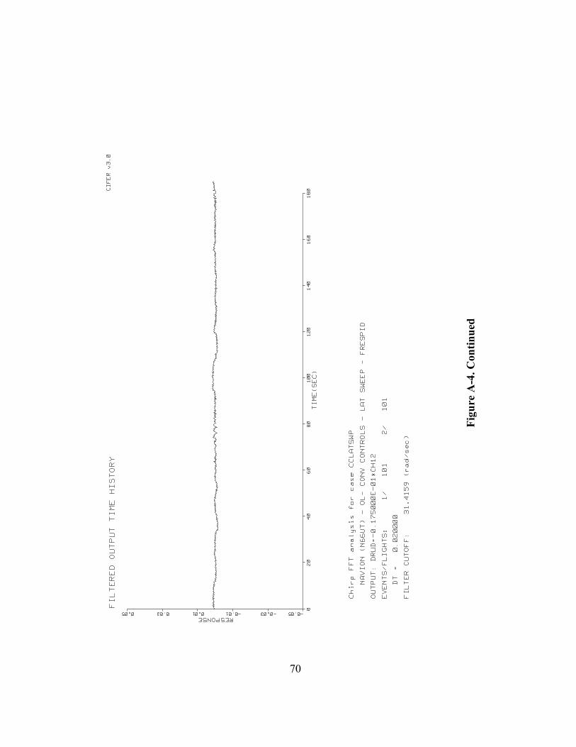
70
Fi
gure
A-4
. Con
tinue
d
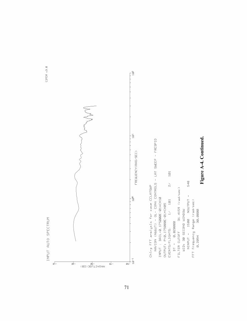
71
Fi
gure
A-4
. Con
tinue
d.
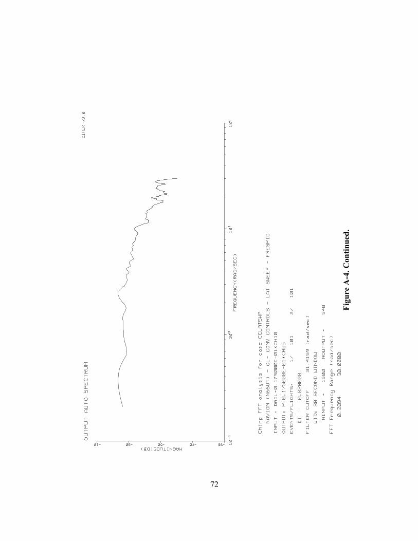
72
Fi
gure
A-4
. Con
tinue
d.

73
Fi
gure
A-4
. Con
tinue
d.
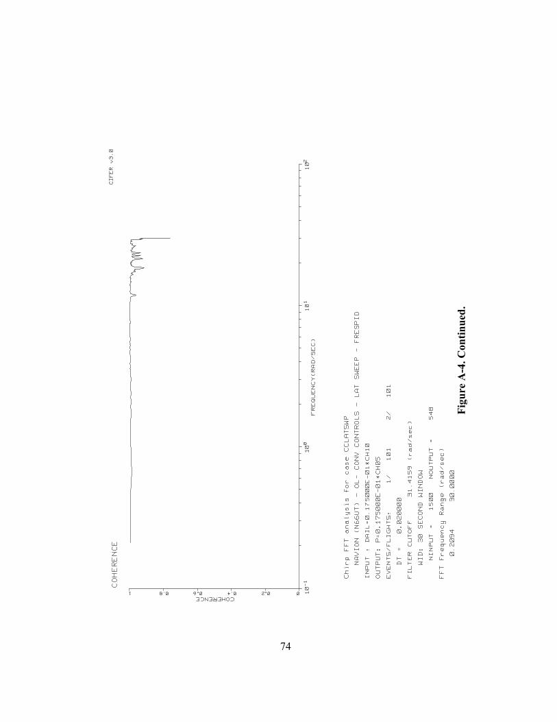
74
Fi
gure
A-4
. Con
tinue
d.
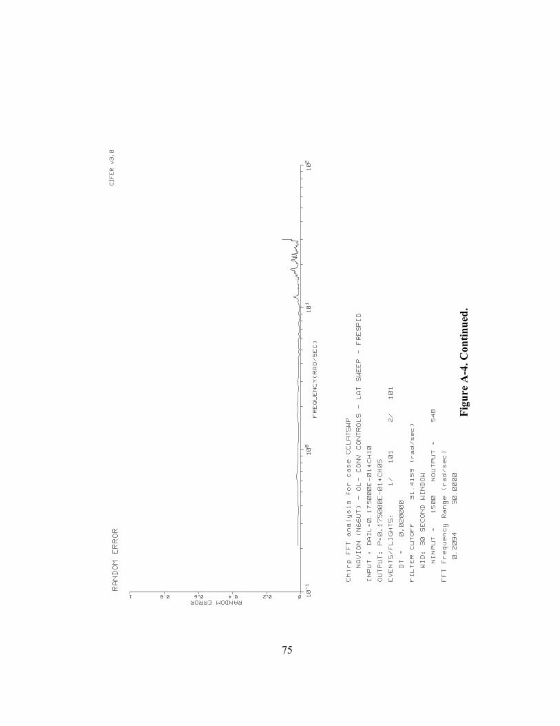
75
Fi
gure
A-4
. Con
tinue
d.

76
Fi
gure
A-4
. Con
tinue
d.
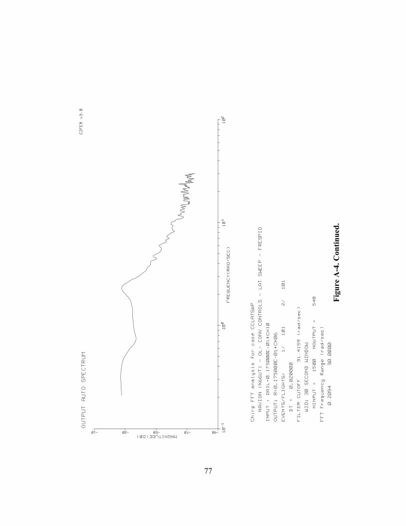
77
Fi
gure
A-4
. Con
tinue
d.
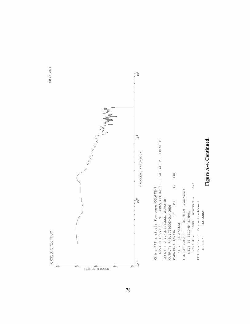
78
Fi
gure
A-4
. Con
tinue
d.
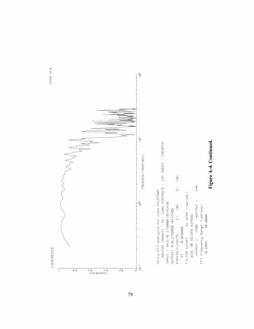
79
Fi
gure
A-4
. Con
tinue
d.
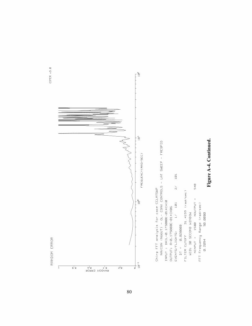
80
Fi
gure
A-4
. Con
tinue
d.

81
Fi
gure
A-4
. Con
tinue
d.

82
Fi
gure
A-4
. Con
tinue
d.
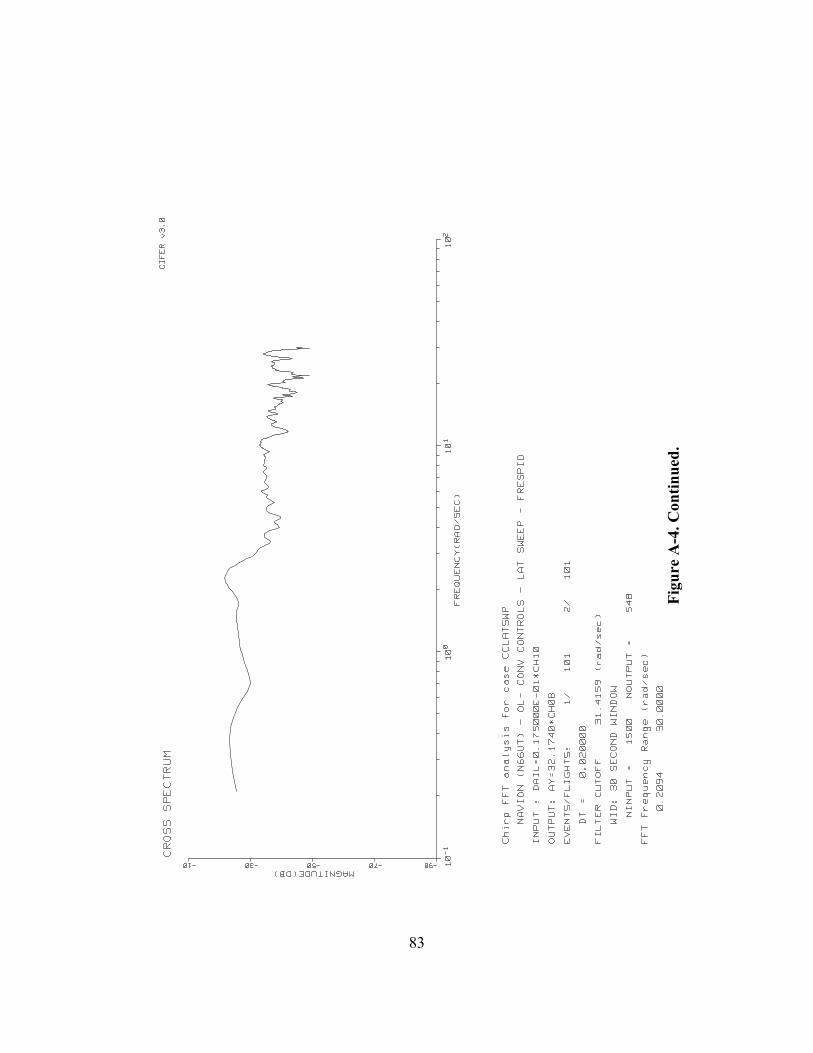
83
Fi
gure
A-4
. Con
tinue
d.
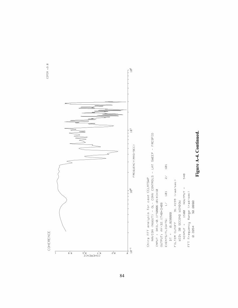
84
Fi
gure
A-4
. Con
tinue
d.
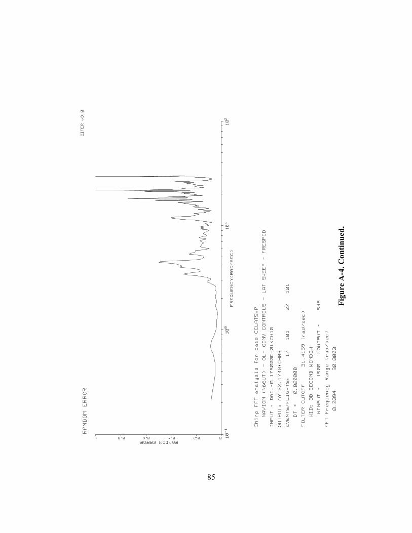
85
Fi
gure
A-4
. Con
tinue
d.

86
Fi
gure
A-4
. Con
tinue
d.
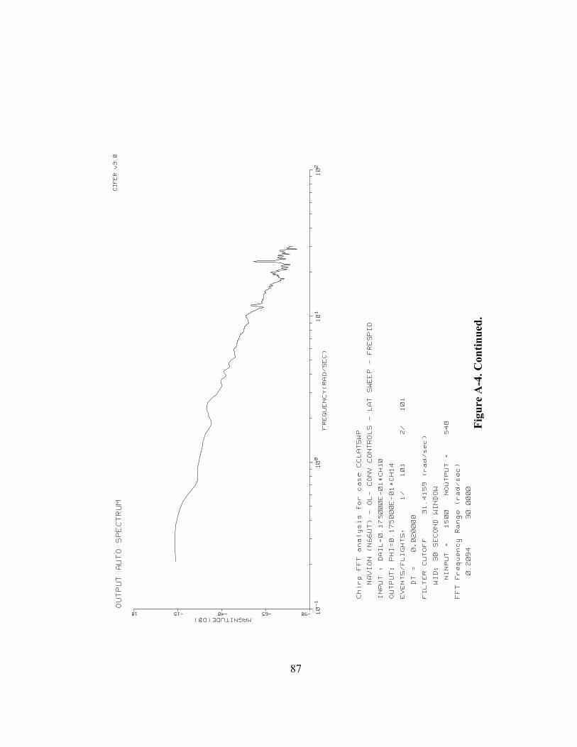
87
Fi
gure
A-4
. Con
tinue
d.
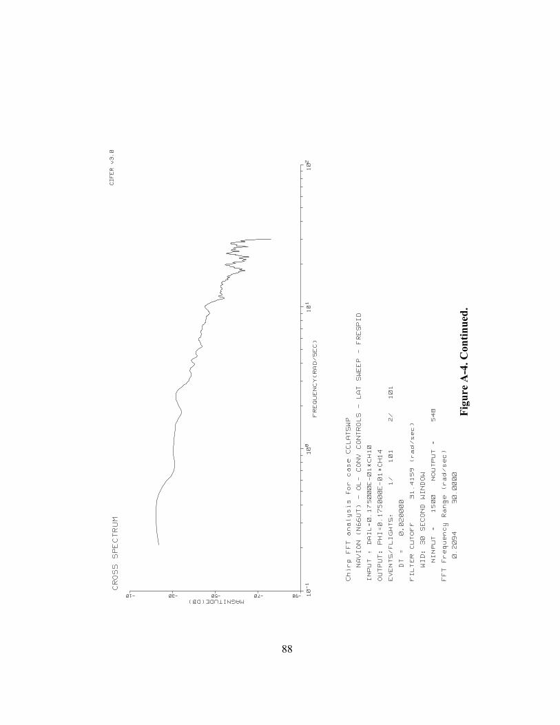
88
Fi
gure
A-4
. Con
tinue
d.
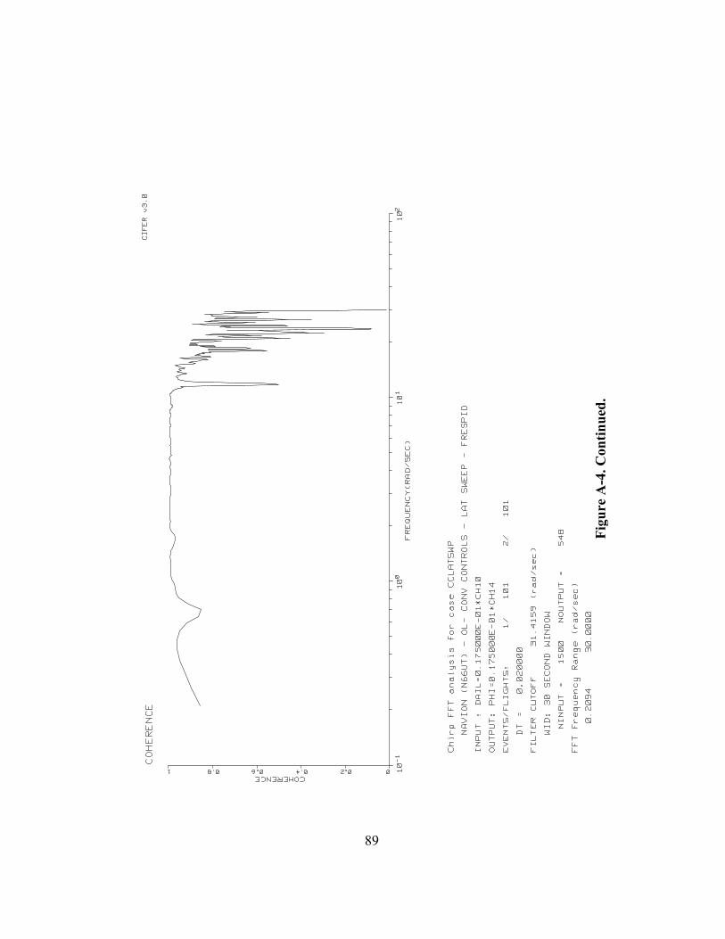
89
Fi
gure
A-4
. Con
tinue
d.
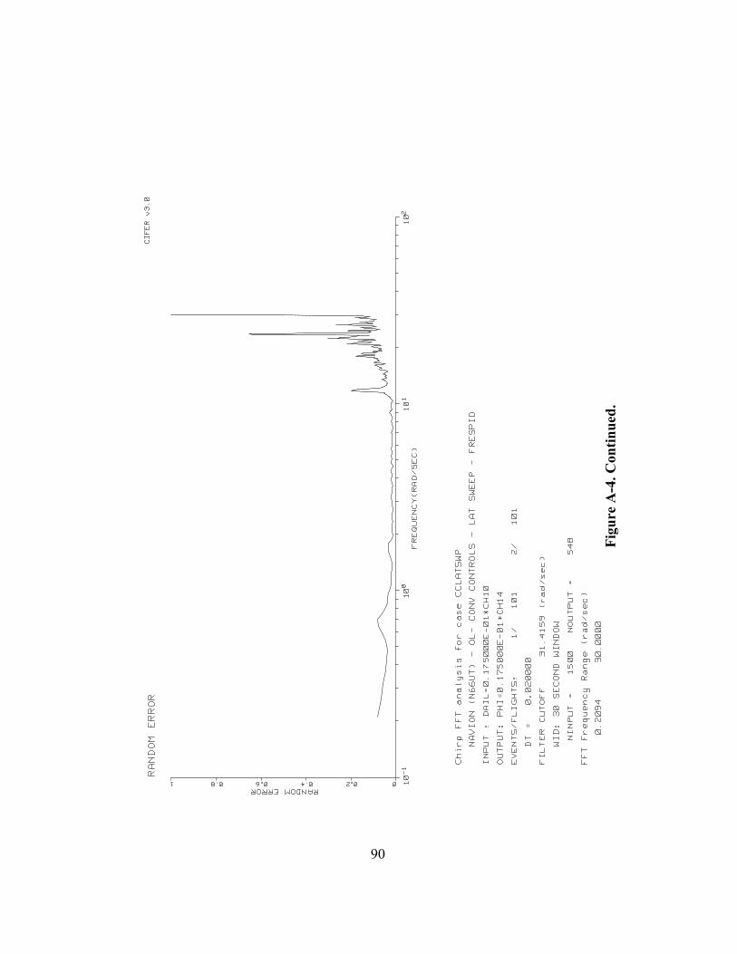
90
Fi
gure
A-4
. Con
tinue
d.
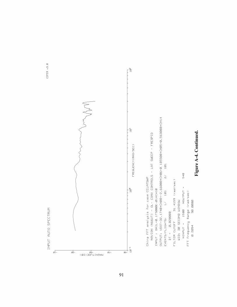
91
Fi
gure
A-4
. Con
tinue
d.
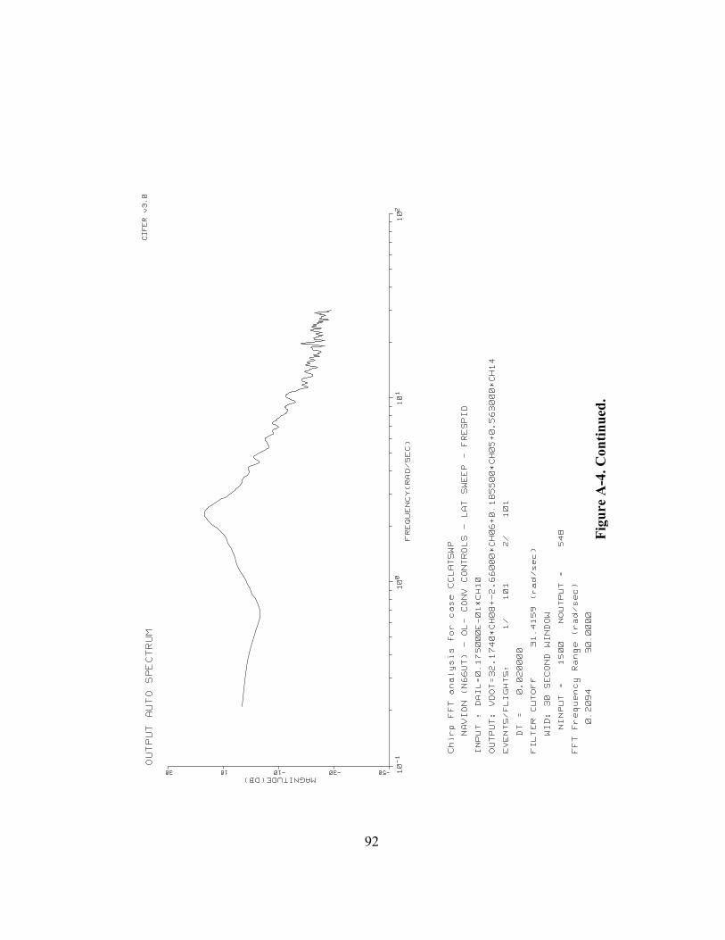
92
Fi
gure
A-4
. Con
tinue
d.
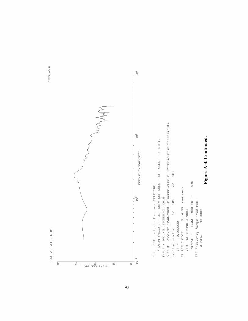
93
Fi
gure
A-4
. Con
tinue
d.
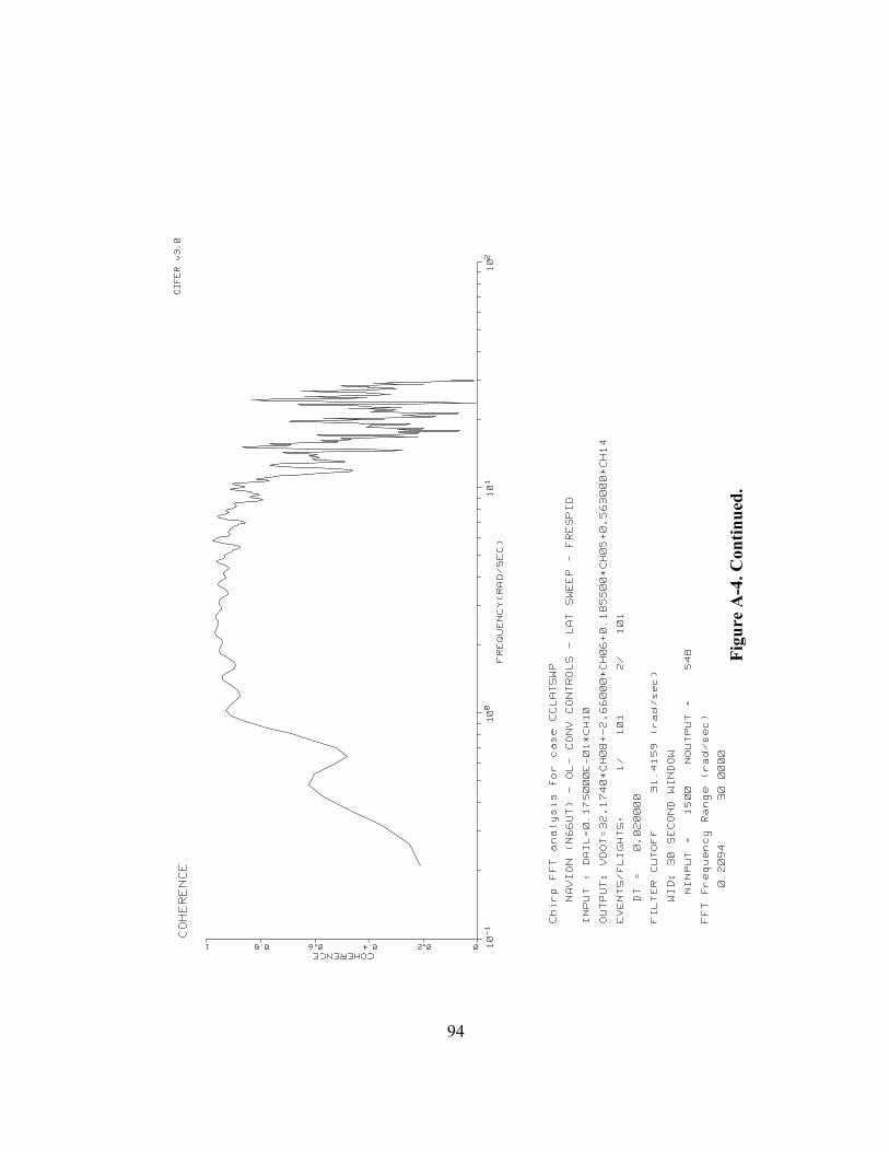
94
Fi
gure
A-4
. Con
tinue
d.
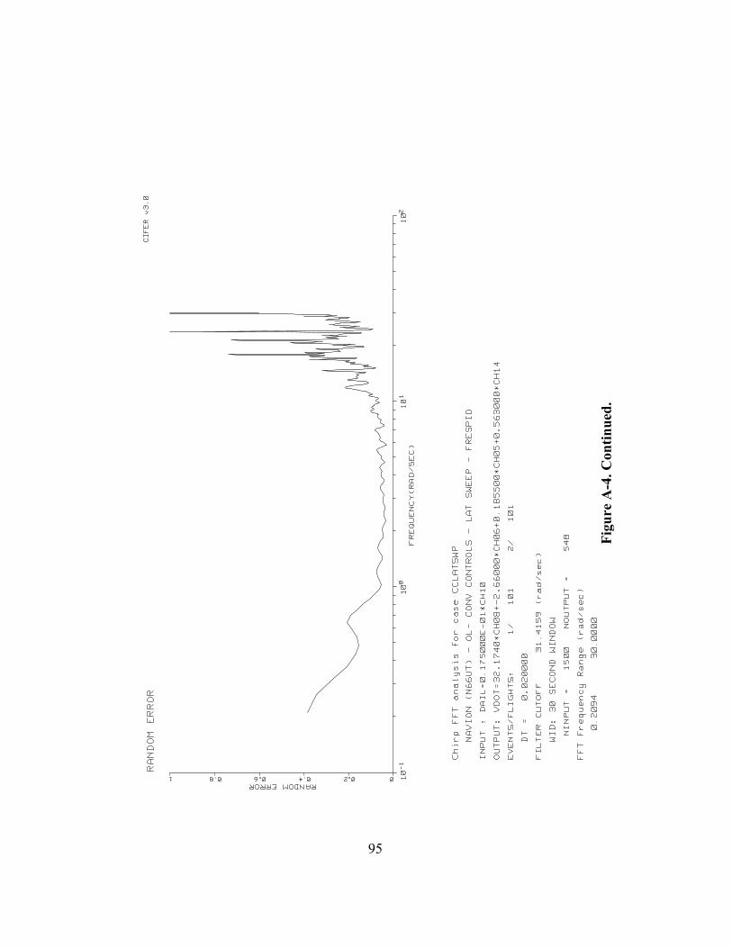
95
Fi
gure
A-4
. Con
tinue
d.

96
Fi
gure
A-4
. Con
tinue
d.
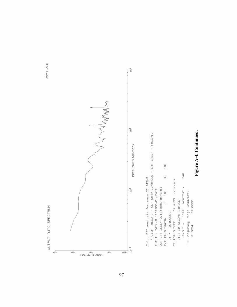
97
Fi
gure
A-4
. Con
tinue
d.
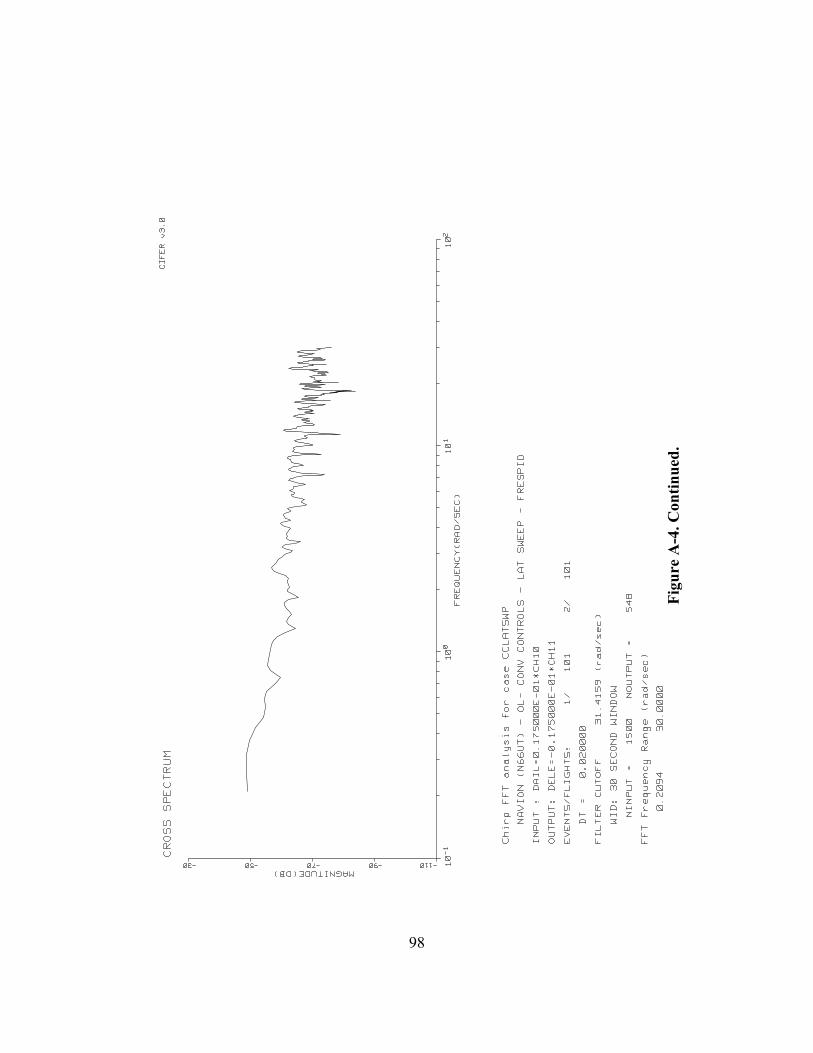
98
Fi
gure
A-4
. Con
tinue
d.
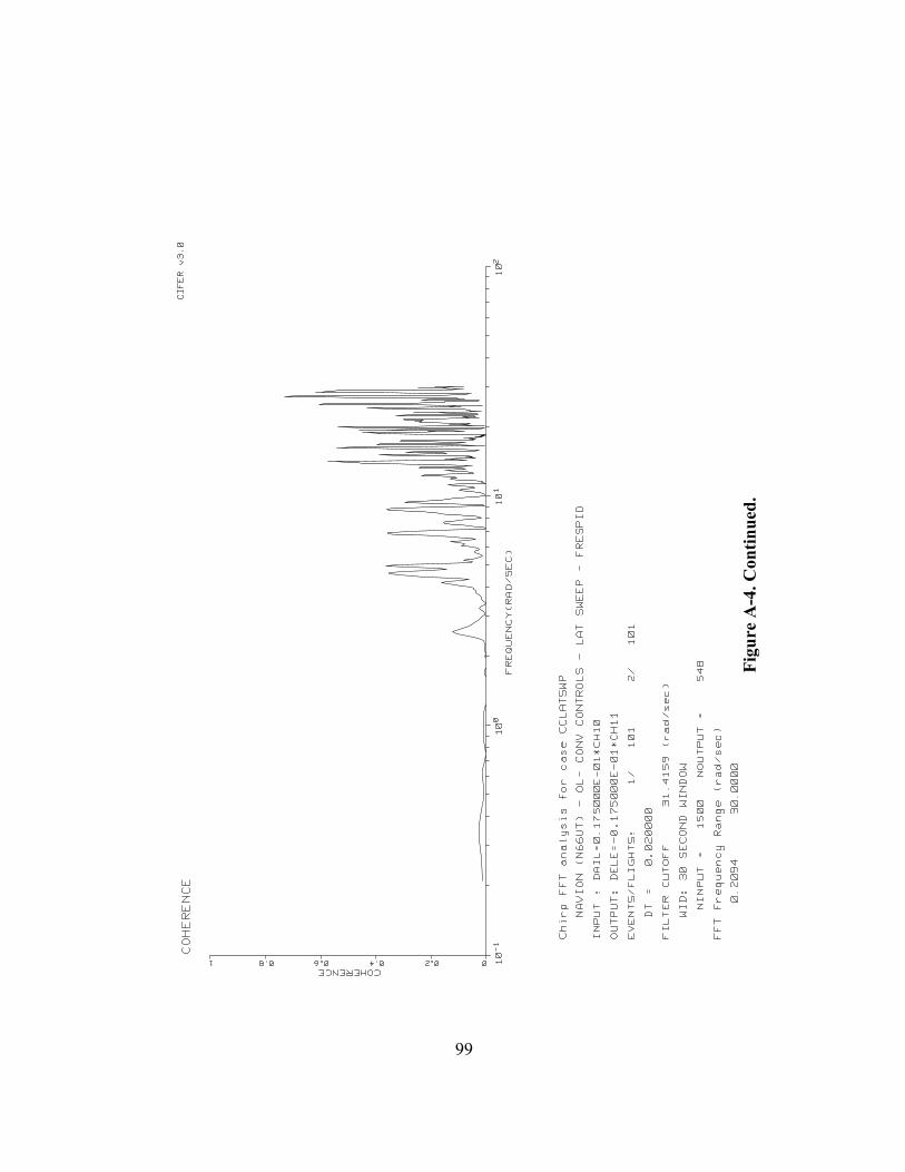
99
Fi
gure
A-4
. Con
tinue
d.
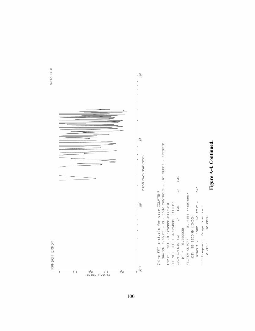
100
Fi
gure
A-4
. Con
tinue
d.
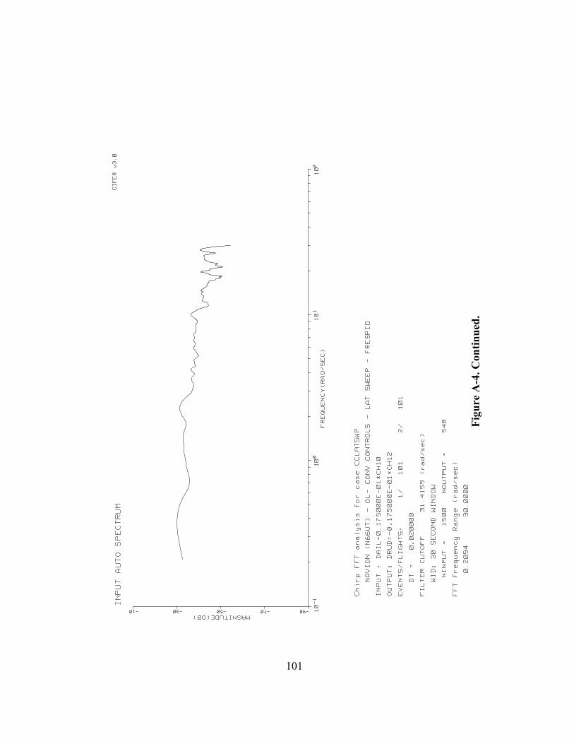
101
Fi
gure
A-4
. Con
tinue
d.
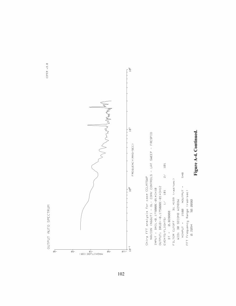
102
Fi
gure
A-4
. Con
tinue
d.
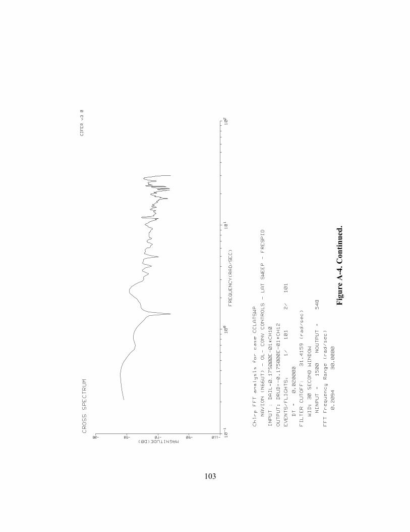
103
Fi
gure
A-4
. Con
tinue
d.
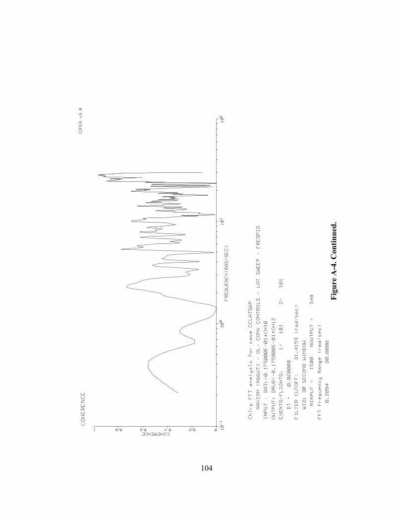
104
Fi
gure
A-4
. Con
tinue
d.
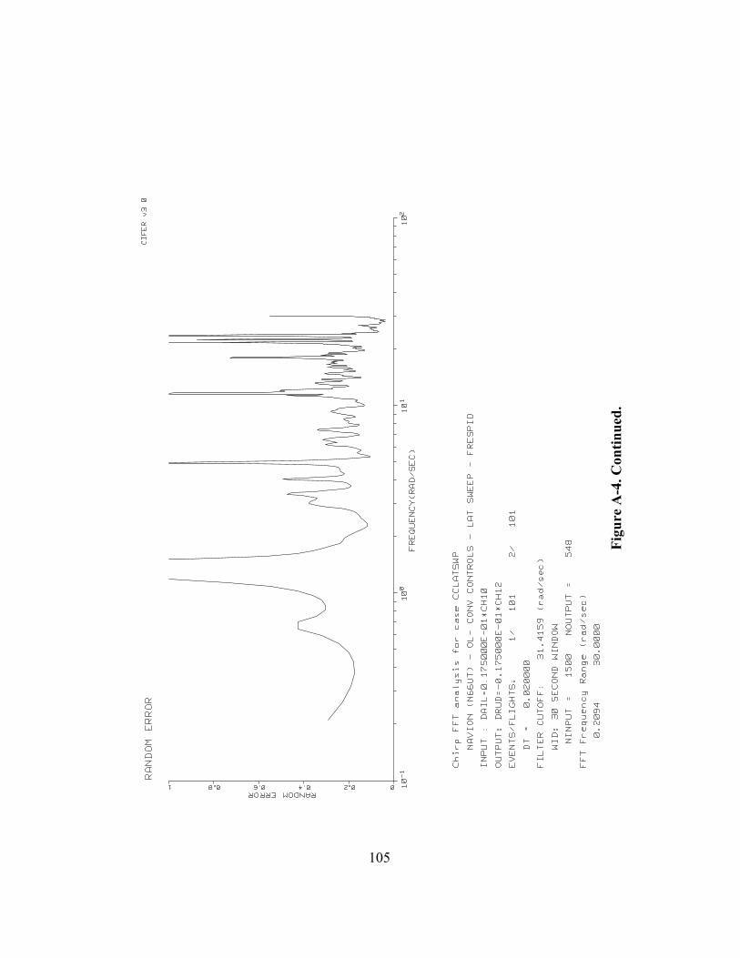
105
Fi
gure
A-4
. Con
tinue
d.
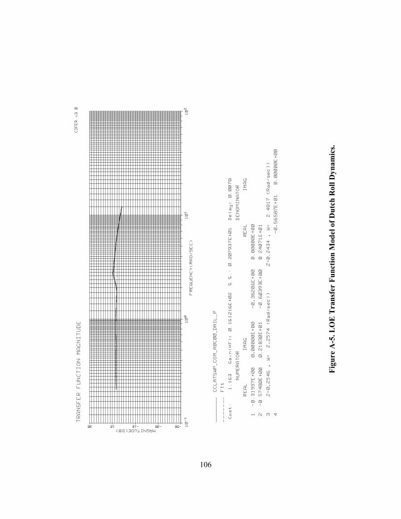
106
Fi
gure
A-5
. LO
E T
rans
fer
Func
tion
Mod
el o
f Dut
ch R
oll D
ynam
ics.
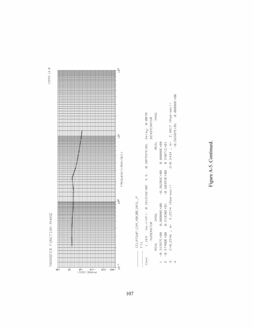
107
Fi
gure
A-5
. Con
tinue
d.
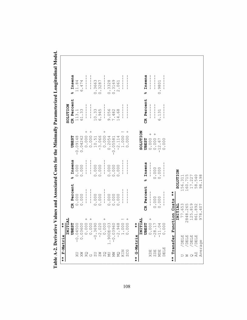
108
Tab
le A
-2. D
eriv
ativ
e V
alue
s and
Ass
ocia
ted
Cos
ts fo
r th
e M
inim
ally
Par
amet
eriz
ed L
ongi
tudi
nal M
odel
. ** F-Matrix **
INITIAL SOLUTION
UBEST CR Percent % Insens UBEST CR Percent % Insens
XU -0.04500 0.000 0.000 -0.09148 113.1 11.84
XW 0.03600 0.000 0.000 0.04242 61.33 6.474
XQ 0.000 + ------ ------ 0.000 + ------ ------
G 0.000 + ------ ------ 0.000 + ------ ------
ZU -0.3690 0.000 0.000 10.51 10.33 0.3663
ZW -2.020 0.000 0.000 -3.066 6.945 0.3287
ZQ 0.000 + ------ ------ 0.000 + ------ ------
MU 1.900E-03 0.000 0.000 0.2054 9.056 0.3328
MW -0.03960 0.000 0.000 -0.05581 7.482 0.3169
MQ -2.948 0.000 0.000 -2.114 14.68 2.061
KIN 1.000 ! ------ ------ 1.000 ! ------ ------
ZCG 0.000 + ------ ------ 0.000 + ------ ------
** G-Matrix **
INITIAL SOLUTION
UBEST CR Percent % Insens UBEST CR Percent % Insens
XDE 0.000 + ------ ------ 0.000 + ------ ------
ZDE -28.17 0.000 0.000 0.000 + ------ ------
MDE -11.04 0.000 0.000 -12.67 6.131 0.9801
DELE 0.000 ------ ------ 0.000 ------ ------
** Transfer Function Costs **
INITIAL SOLUTION
U /DELE 77.653 156.311
W /DELE 2848.265 160.715
Q /DELE 125.819 17.227
AZ /DELE 861.892 58.540
Average 978.407 98.198
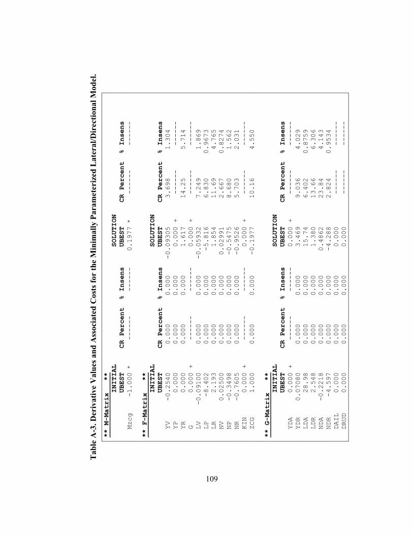
109
Tab
le A
-3. D
eriv
ativ
e V
alue
s and
Ass
ocia
ted
Cos
ts fo
r th
e M
inim
ally
Par
amet
eriz
ed L
ater
al/D
irec
tiona
l Mod
el.
** M-Matrix **
INITIAL SOLUTION
UBEST CR Percent % Insens UBEST CR Percent % Insens
Mzcg -1.000 * ------ ------ 0.1977 * ------ ------
** F-Matrix **
INITIAL SOLUTION
UBEST CR Percent % Insens UBEST CR Percent % Insens
YV -0.2540 0.000 0.000 -0.09305 3.698 1.304
YP 0.000 0.000 0.000 0.000 + ------ ------
YR 0.000 0.000 0.000 1.617 14.25 5.714
G 0.000 + ------ ------ 0.000 + ------ ------
LV -0.09100 0.000 0.000 -0.05932 7.249 1.869
LP -8.402 0.000 0.000 -5.816 6.830 0.9673
LR 2.193 0.000 0.000 1.854 11.69 4.765
NV 0.02500 0.000 0.000 0.02991 2.667 0.8274
NP -0.3498 0.000 0.000 -0.5475 8.680 1.562
NR -0.7605 0.000 0.000 -0.9526 5.703 2.031
KIN 0.000 + ------ ------ 0.000 + ------ ------
ZCG 1.000 0.000 0.000 -0.1977 10.16 4.550
** G-Matrix **
INITIAL SOLUTION
UBEST CR Percent % Insens UBEST CR Percent % Insens
YDA 0.000 + ------ ------ 0.000 + ------ ------
YDR 0.07080 0.000 0.000 3.469 9.036 4.029
LDA 28.98 0.000 0.000 15.74 6.402 0.8759
LDR 2.548 0.000 0.000 1.380 13.66 6.306
NDA -0.2218 0.000 0.000 0.4862 23.84 4.143
NDR -4.597 0.000 0.000 -4.288 2.824 0.9534
DAIL 0.000 0.000 0.000 0.000 ------ ------
DRUD 0.000 0.000 0.000 0.000 ------ ------
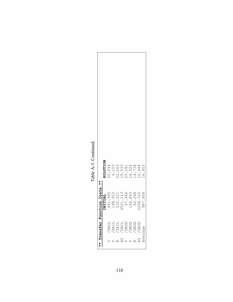
110
Tabl
e A
-3. C
ontin
ued.
** Transfer Function Costs **
INITIAL SOLUTION
V /DAIL 441.385 22.034
P /DAIL 148.912 4.103
R /DAIL 232.521 22.563
AY /DAIL 4521.113 19.533
V /DRUD 67.466 25.191
P /DRUD 166.893 16.522
R /DRUD 62.248 14.734
AY /DRUD 2258.725 10.944
Average 987.408 16.953
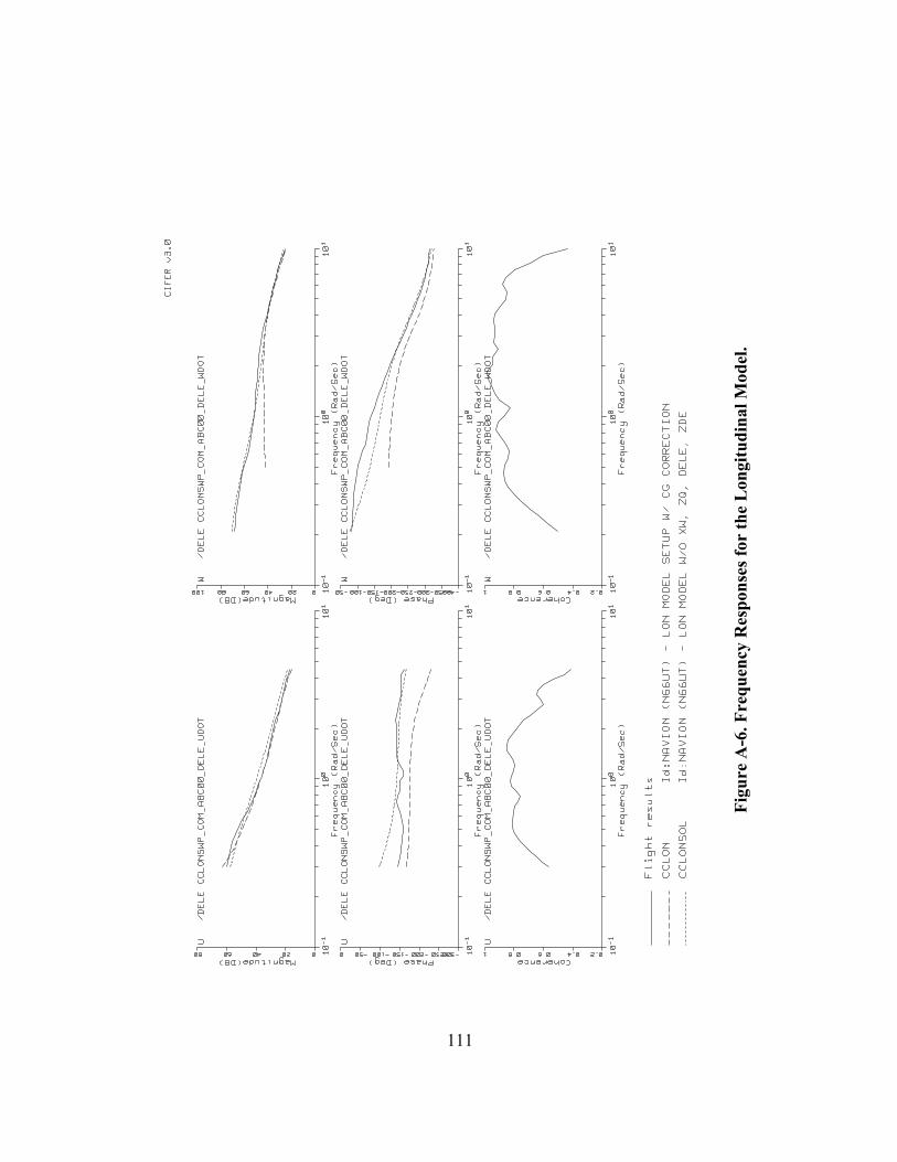
111
Fi
gure
A-6
. Fre
quen
cy R
espo
nses
for
the
Lon
gitu
dina
l Mod
el.
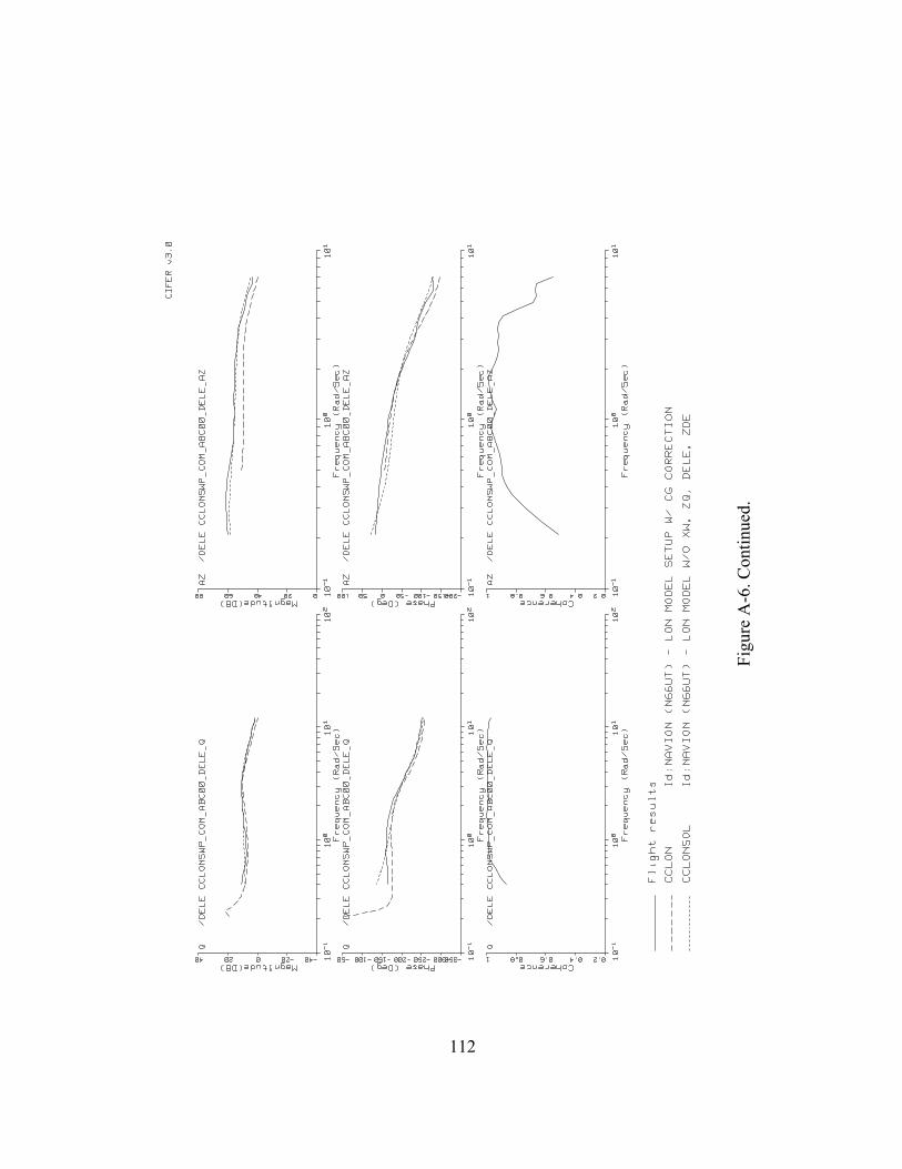
112
Fi
gure
A-6
. Con
tinue
d.
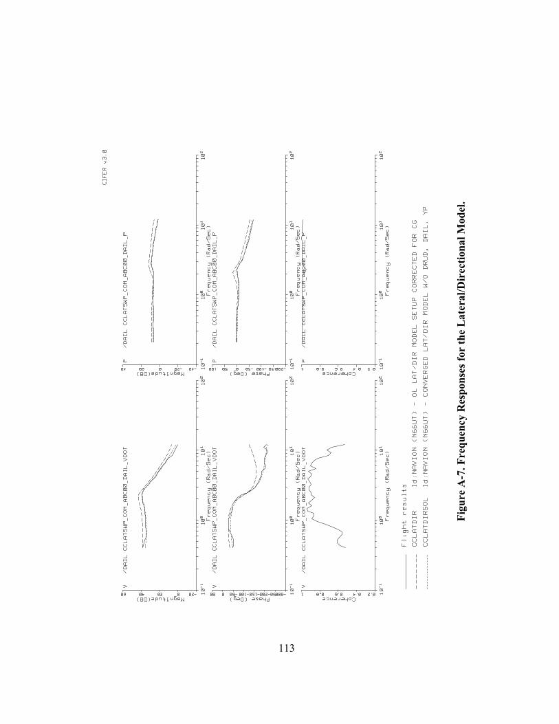
113
Fi
gure
A-7
. Fre
quen
cy R
espo
nses
for
the
Lat
eral
/Dir
ectio
nal M
odel
.
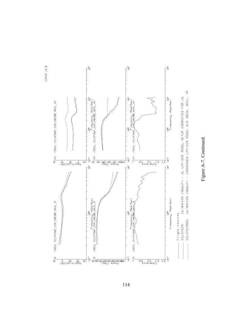
114
Fi
gure
A-7
. Con
tinue
d.
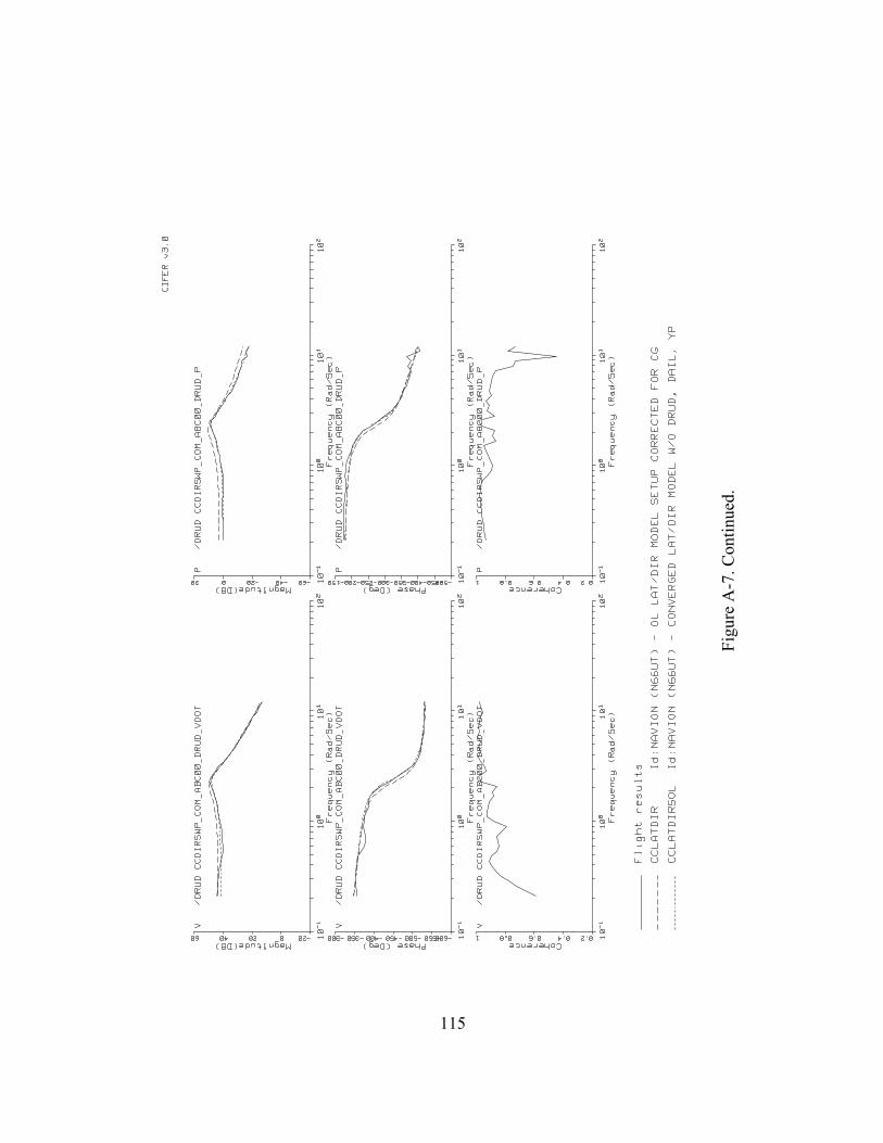
115
Fi
gure
A-7
. Con
tinue
d.
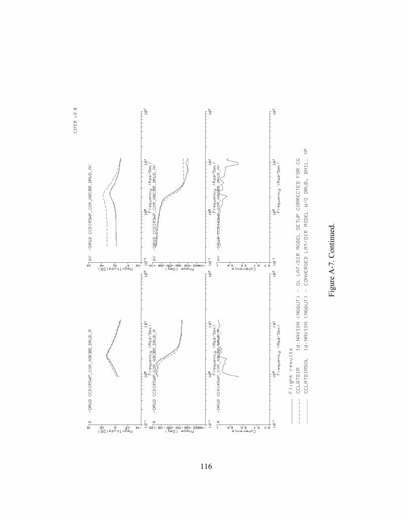
116
Fi
gure
A-7
. Con
tinue
d.
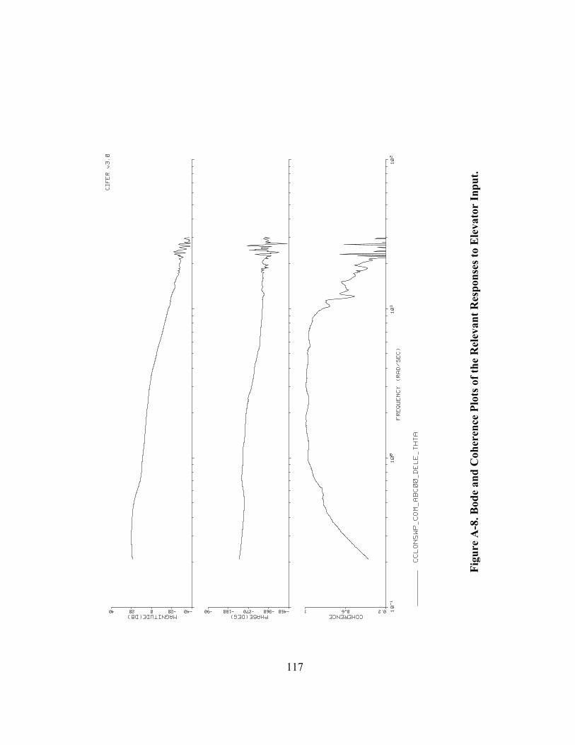
117
Fi
gure
A-8
. Bod
e an
d C
oher
ence
Plo
ts o
f the
Rel
evan
t Res
pons
es to
Ele
vato
r In
put.
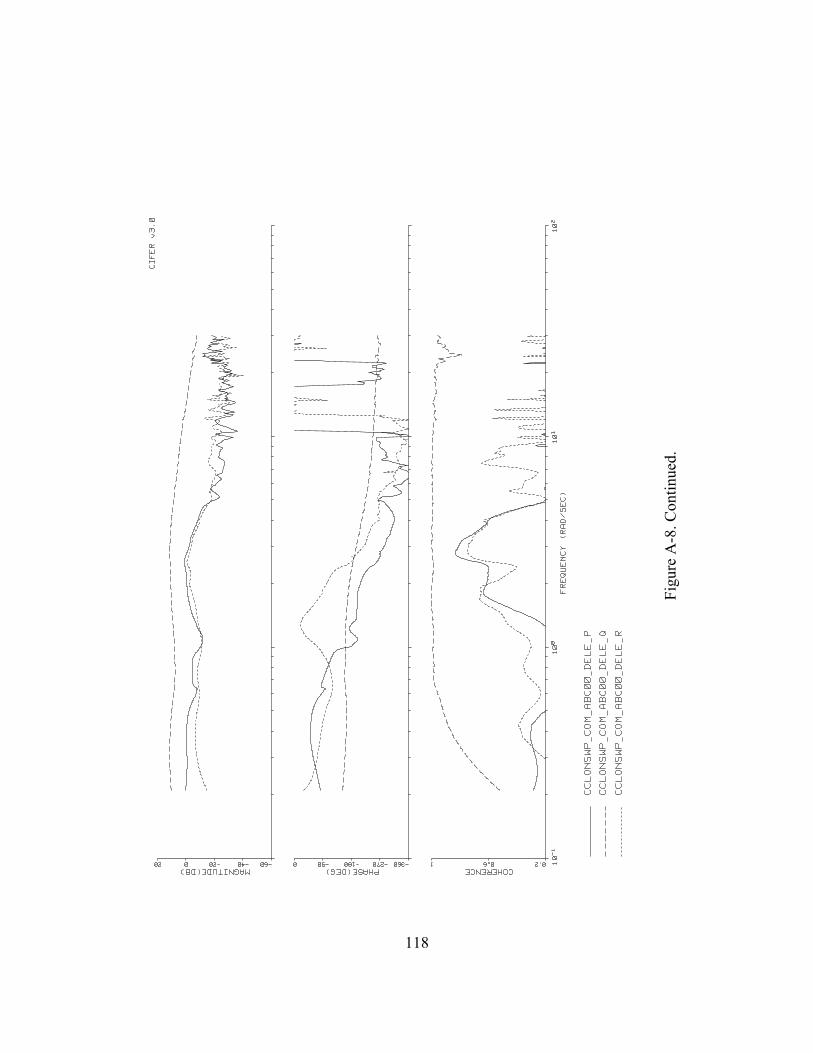
118
Fi
gure
A-8
. Con
tinue
d.
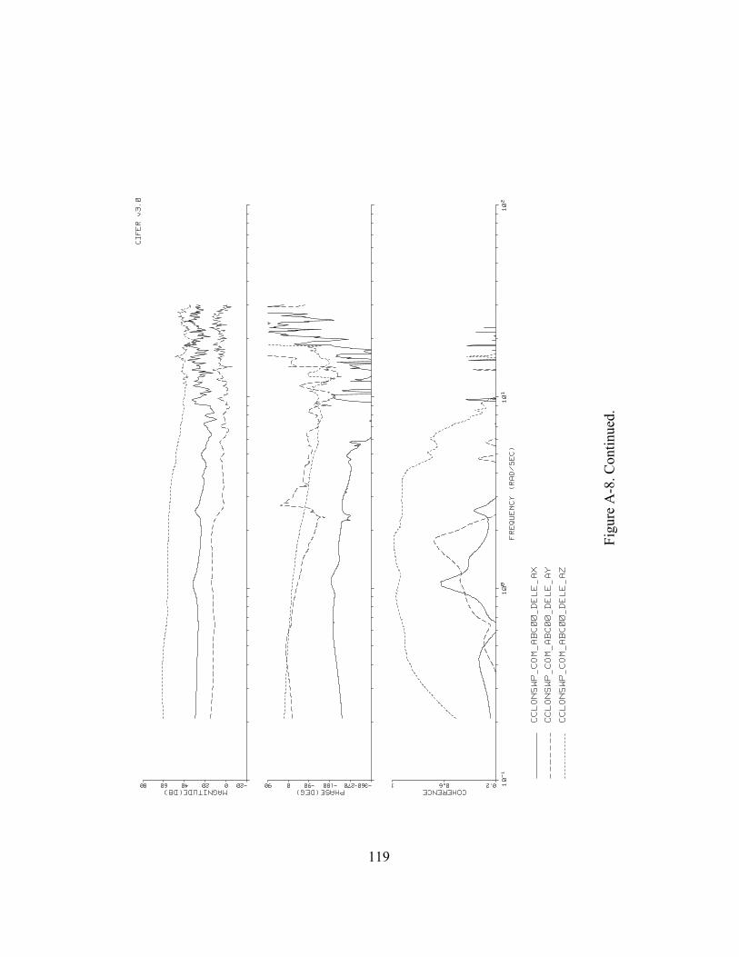
119
Fi
gure
A-8
. Con
tinue
d.
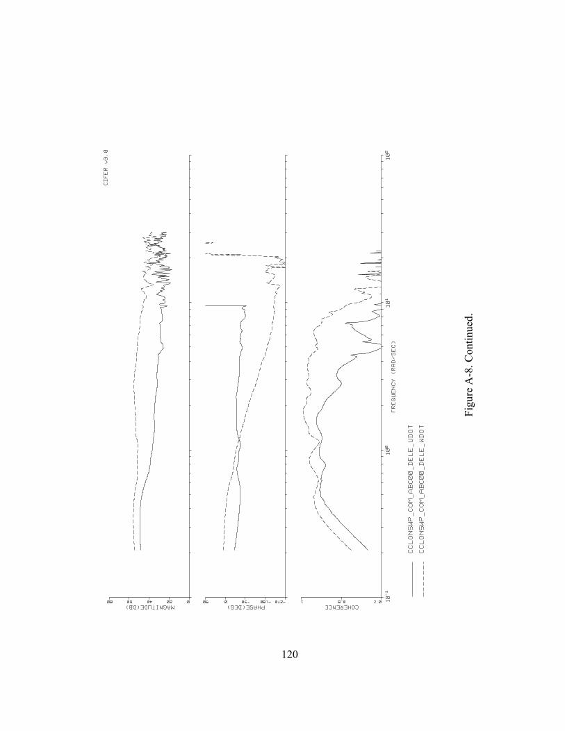
120
Fi
gure
A-8
. Con
tinue
d.
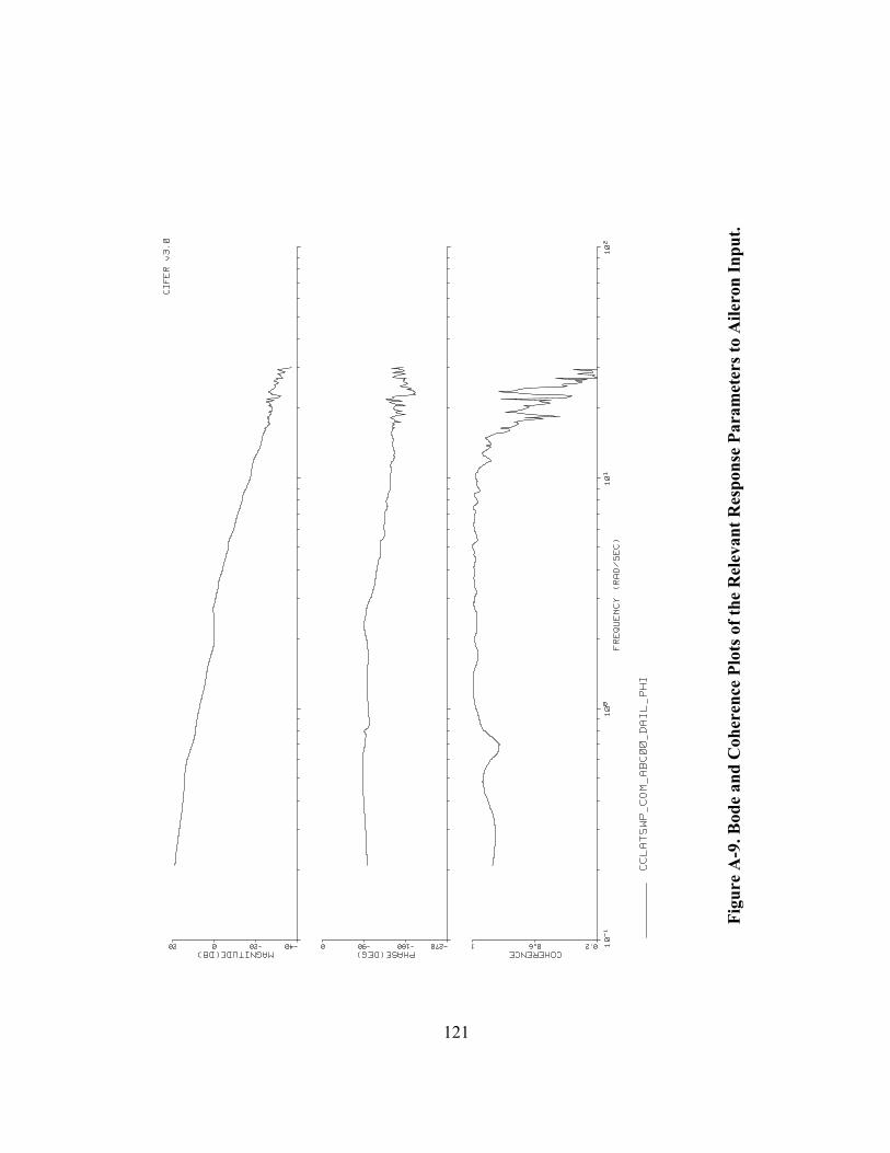
121
Fi
gure
A-9
. Bod
e an
d C
oher
ence
Plo
ts o
f the
Rel
evan
t Res
pons
e Pa
ram
eter
s to
Aile
ron
Inpu
t.
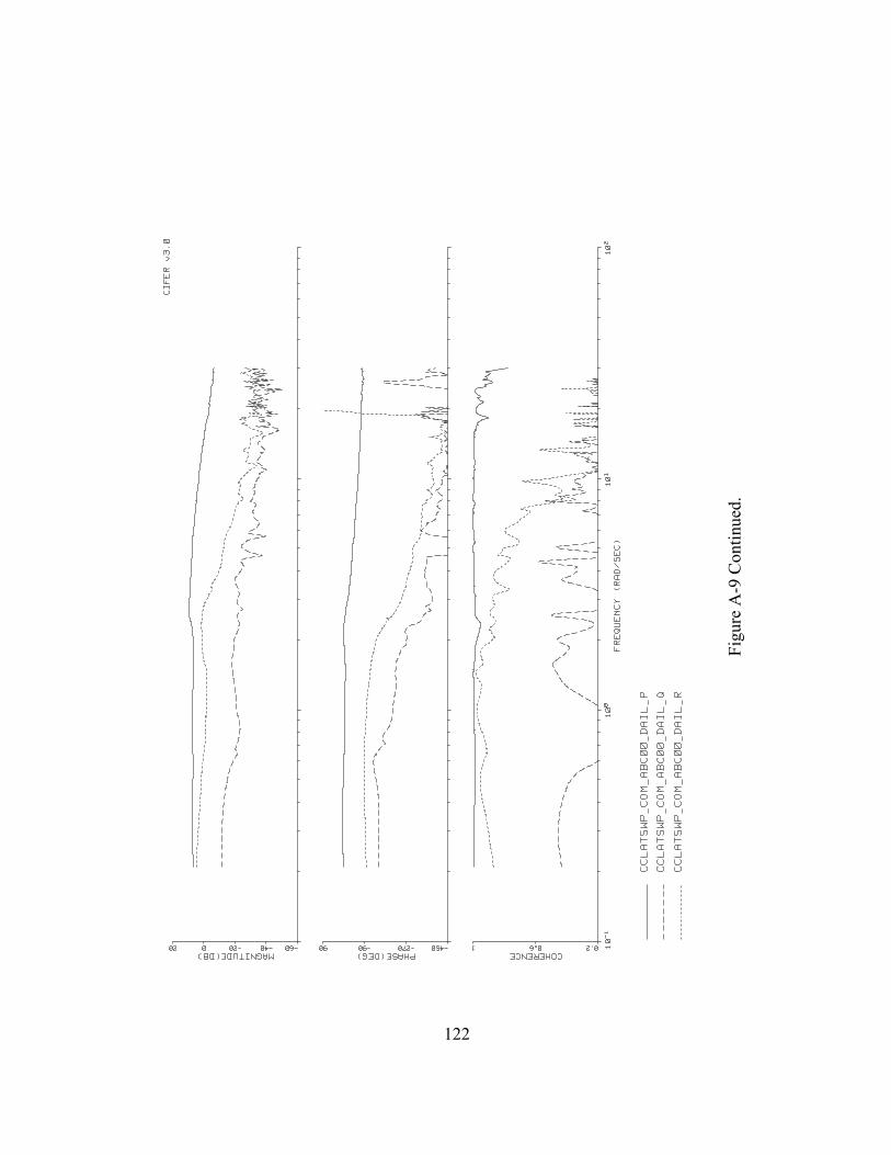
122
Fi
gure
A-9
Con
tinue
d.
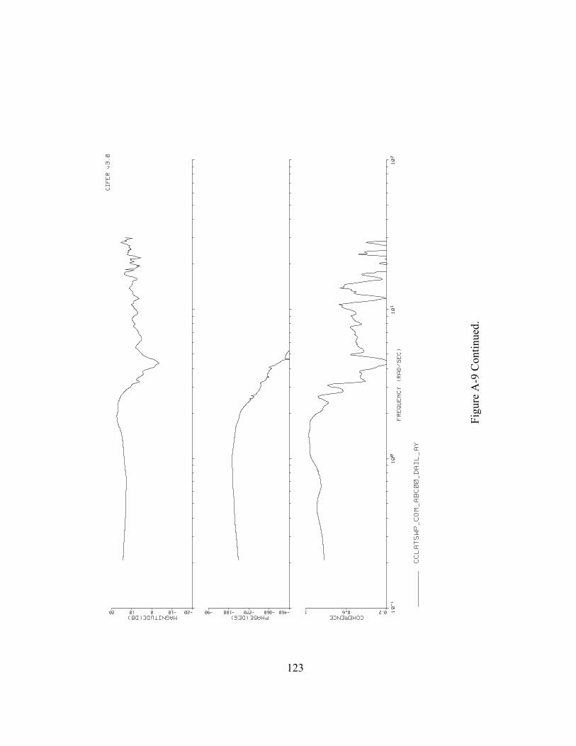
123
Fi
gure
A-9
Con
tinue
d.
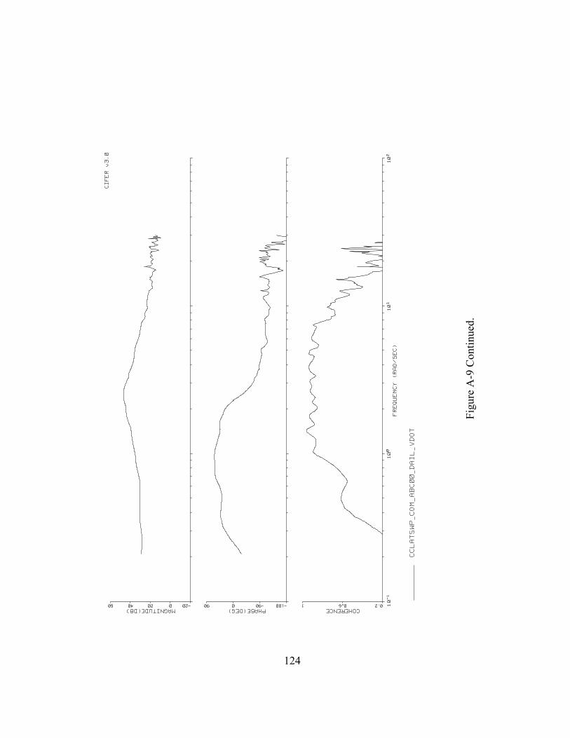
124
Fi
gure
A-9
Con
tinue
d.
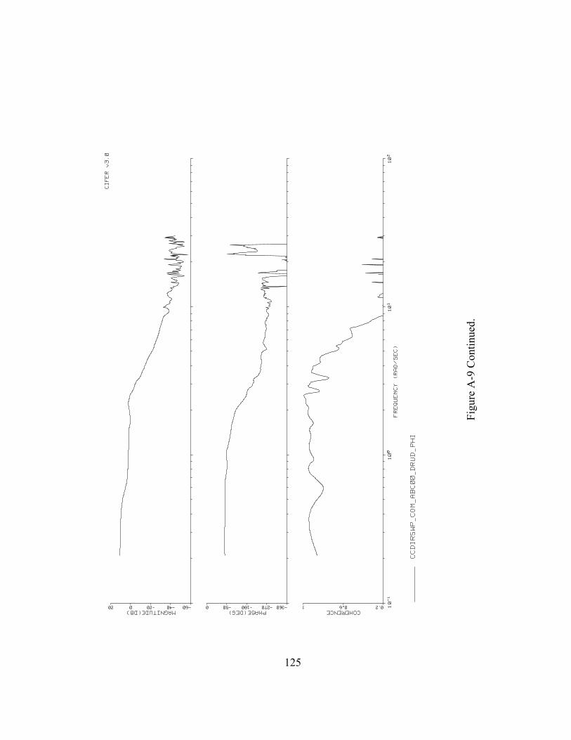
125
Fi
gure
A-9
Con
tinue
d.
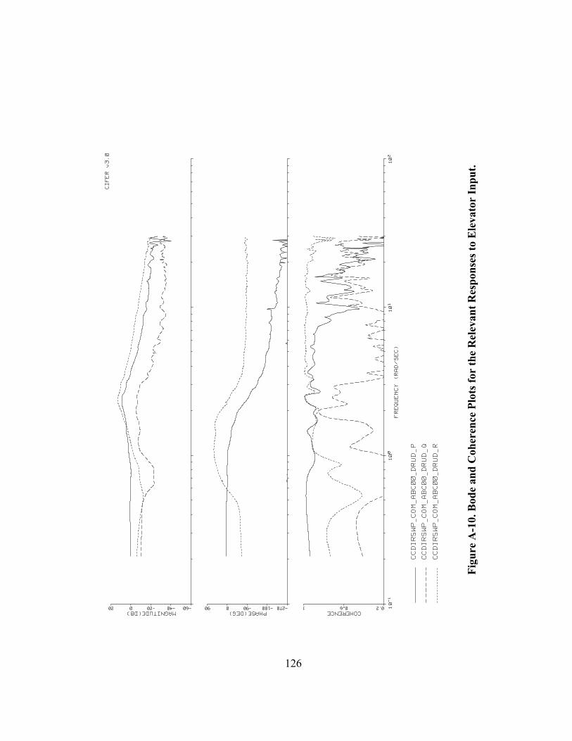
126
Fi
gure
A-1
0. B
ode
and
Coh
eren
ce P
lots
for
the
Rel
evan
t Res
pons
es to
Ele
vato
r In
put.
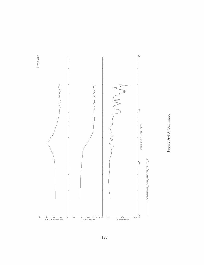
127
Fi
gure
A-1
0. C
ontin
ued.
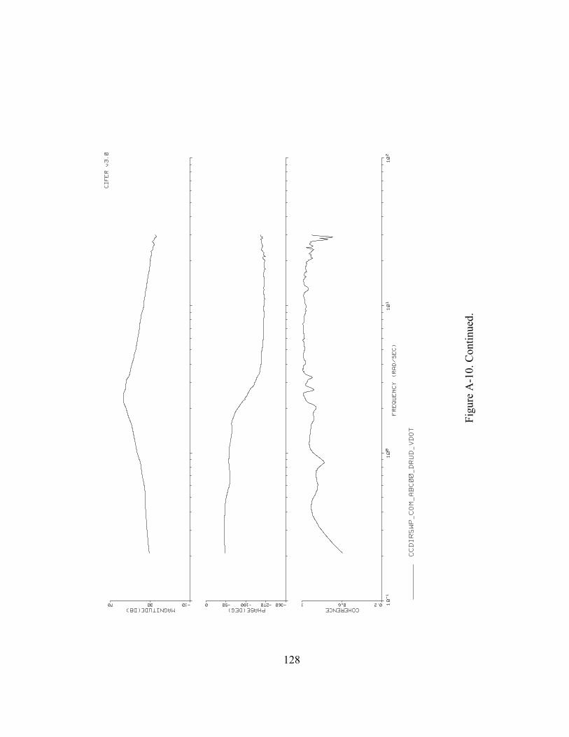
128
Fi
gure
A-1
0. C
ontin
ued.
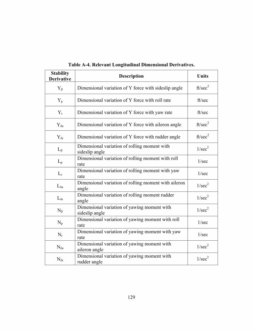
129
Table A-4. Relevant Longitudinal Dimensional Derivatives.
Stability Derivative Description Units
Yβ Dimensional variation of Y force with sideslip angle ft/sec2
Yp Dimensional variation of Y force with roll rate ft/sec
Yr Dimensional variation of Y force with yaw rate ft/sec
Yδa Dimensional variation of Y force with aileron angle ft/sec2
Yδr Dimensional variation of Y force with rudder angle ft/sec2
Lβ Dimensional variation of rolling moment with sideslip angle 1/sec2
Lp Dimensional variation of rolling moment with roll rate 1/sec
Lr Dimensional variation of rolling moment with yaw rate 1/sec
Lδa Dimensional variation of rolling moment with aileron angle 1/sec2
Lδr Dimensional variation of rolling moment rudder angle 1/sec2
Nβ Dimensional variation of yawing moment with sideslip angle 1/sec2
Np Dimensional variation of yawing moment with roll rate 1/sec
Nr Dimensional variation of yawing moment with yaw rate 1/sec
Nδa Dimensional variation of yawing moment with aileron angle 1/sec2
Nδr Dimensional variation of yawing moment with rudder angle 1/sec2
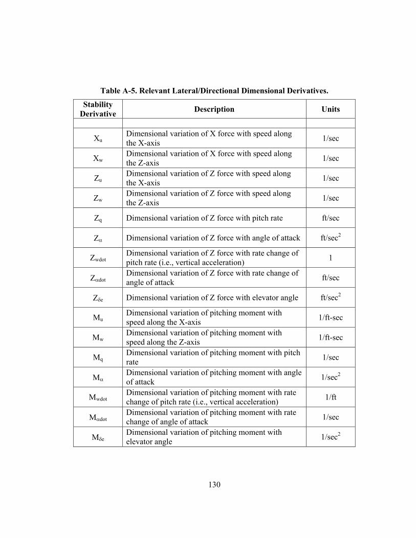
130
Table A-5. Relevant Lateral/Directional Dimensional Derivatives.
Stability Derivative Description Units
Xu Dimensional variation of X force with speed along the X-axis 1/sec
Xw Dimensional variation of X force with speed along the Z-axis 1/sec
Zu Dimensional variation of Z force with speed along the X-axis 1/sec
Zw Dimensional variation of Z force with speed along the Z-axis 1/sec
Zq Dimensional variation of Z force with pitch rate ft/sec
Zα Dimensional variation of Z force with angle of attack ft/sec2
Zwdot Dimensional variation of Z force with rate change of pitch rate (i.e., vertical acceleration) 1
Zαdot Dimensional variation of Z force with rate change of angle of attack ft/sec
Zδe Dimensional variation of Z force with elevator angle ft/sec2
Mu Dimensional variation of pitching moment with speed along the X-axis 1/ft-sec
Mw Dimensional variation of pitching moment with speed along the Z-axis 1/ft-sec
Mq Dimensional variation of pitching moment with pitch rate 1/sec
Mα Dimensional variation of pitching moment with angle of attack 1/sec2
Mwdot Dimensional variation of pitching moment with rate change of pitch rate (i.e., vertical acceleration) 1/ft
Mαdot Dimensional variation of pitching moment with rate change of angle of attack 1/sec
Mδe Dimensional variation of pitching moment with elevator angle 1/sec2
131
VITA
Robert Charles Catterall was born in Rockford, Illinois, on May 23, 1974. In 1986 he
moved to Mt. Juliet, Tennessee, where he later graduated from Mt. Juliet Christian
Academy in 1992. Thereafter, he attended Tennessee Technological University, in
Cookeville, Tennessee, where he received a Bachelor of Science in Mechanical
Engineering with a minor in Mathematics in 1997. From there, he attended the
University of Tennessee Space Institute (UTSI), in Tullahoma, Tennessee, to pursue a
Master of Science degree, with a major in Aviation Systems.
Robert is currently a Sr. Engineer with the Enabling Technologies group at Delta Air
Lines, in Atlanta, Georgia.
Recommended