STAT3011 STOCHASTIC PROCESSES AND TIME SERIES
COURSE NOTES
1
Contents Introduction: ........................................................................................................................................... 6
Assessments: ....................................................................................................................................... 6
Schedule: ............................................................................................................................................. 6
Stochastic Processes: .............................................................................................................................. 7
Basic concenpts: .................................................................................................................................. 8
Definition: Stochastic process ......................................................................................................... 8
Definition: Random walk ................................................................................................................. 9
Definition: Strong stationary ........................................................................................................... 9
Definition: State space of stochastic process ................................................................................. 9
Definition: Increments .................................................................................................................... 9
Markov Property: .............................................................................................................................. 10
Definition: Markov property ......................................................................................................... 11
Definition: filtration ...................................................................................................................... 12
Definition: Markov Process ........................................................................................................... 12
Markov Chains ...................................................................................................................................... 12
Basic concepts: .................................................................................................................................. 13
Notation: ....................................................................................................................................... 13
Gambler ruin problem: ..................................................................................................................... 13
Solution ......................................................................................................................................... 14
Classification of states: ..................................................................................................................... 15
𝑛 step transition probability notation: ......................................................................................... 15
Recurrence and transience ............................................................................................................... 19
Recurrence definition: .................................................................................................................. 19
Transient definition: ...................................................................................................................... 19
Green Function: ............................................................................................................................ 19
Period: ........................................................................................................................................... 22
Limiting theorems and Stationarity of Markov Chains ......................................................................... 25
Expected number of transitions from 𝑗 to 𝑗...................................................................................... 25
Definition: ..................................................................................................................................... 25
Number of visits to 𝑗 by the 𝑛𝑡ℎ step: .......................................................................................... 25
Stationary Distributions .................................................................................................................... 29
Discussion: .................................................................................................................................... 29
Set up: ........................................................................................................................................... 30
Theorem: irreducible aperiodic Markov chains and classes: ........................................................ 30
Poisson Processes ................................................................................................................................. 34

2
Introduction: ..................................................................................................................................... 34
Theory from notes: ....................................................................................................................... 35
Revision of Distributions ................................................................................................................... 36
Poisson distribution ...................................................................................................................... 36
Exponential Distribution ............................................................................................................... 37
Definition of Poisson Process: ........................................................................................................... 39
Counting process (definition) ........................................................................................................ 39
Poisson Process Definition: ........................................................................................................... 40
Interarrival and waiting time distributions: ...................................................................................... 41
Distribution of 𝐸𝑘: Interarrival time ............................................................................................. 41
Distribution of 𝑇𝑘: Waiting time ................................................................................................... 42
Conditional Distribution of the Arrival Times ............................................................................... 43
Superposition and Thinning of Poisson Processes ............................................................................ 46
Theorem: Superposition position of Poisson Processes: .............................................................. 46
Sampling (thinning) ....................................................................................................................... 47
Revision: ................................................................................................................................................ 49
Random Sums (STAT2911) ................................................................................................................ 49
Examples: ...................................................................................................................................... 49
STAT3911 Random sums: .............................................................................................................. 51
Moment Generating Function .......................................................................................................... 52
Definition: ..................................................................................................................................... 52
Calculating MGF: ........................................................................................................................... 52
Moment Generating function of a random Sum .......................................................................... 56
Branching Processes: ............................................................................................................................ 57
Set up: ............................................................................................................................................... 58
Class .............................................................................................................................................. 58
Notes: ............................................................................................................................................ 59
Formulation of branching process: ................................................................................................... 59
Expectation and variance of 𝑍𝑛 + 1 ............................................................................................. 60
Probability of dying out: ................................................................................................................ 61
Brownian motion .............................................................................................................................. 68
Definition 1.................................................................................................................................... 68
Definition 2.................................................................................................................................... 69
Time Series: ........................................................................................................................................... 69
Basic concepts: .................................................................................................................................. 71
Regular time seris: ........................................................................................................................ 71

3
Notation for TS data: ..................................................................................................................... 71
Graphs of Time Series Data ........................................................................................................... 73
Basic Terminology of TS analysis ................................................................................................... 80
Analysis of Components of time series: ............................................................................................ 82
Estimation and elimination of trend in absence of seasonality: ................................................... 82
Estimation and elimination of both trend and seasonal components of a TS .............................. 89
Stationary Processes and Time Series 1: ............................................................................................... 91
Autocovariance and Autocorrelation Functions ............................................................................... 92
Definition: autocovariance function 𝛾 .......................................................................................... 92
Definition: Autocorrelation (acf) 𝜌 ............................................................................................... 93
Estimation of 𝛾𝑘 and 𝜌𝑘 ............................................................................................................... 93
Sampling Properties of 𝑋𝑛; 𝐶𝑛, 𝑘; 𝑅𝑛, 𝑘 ........................................................................................... 95
Sampling properties of 𝑋𝑛 ............................................................................................................ 95
Sampling properties of 𝐶𝑛, 𝑘 ........................................................................................................ 96
Sampling properties for 𝑅𝑛, 𝑘 ....................................................................................................... 96
Sample Correlogram ..................................................................................................................... 97
Detection of Randomness, short term and long term correlations of a TS .................................. 98
Autocorrelation Plot as Diagnostic Tool ..................................................................................... 101
Partial Autocorrelation Function (PACF) ..................................................................................... 103
Stationary Time Series: ............................................................................................................... 104
Some Stochastic Models for Time Series ............................................................................................ 104
White Noise Process ....................................................................................................................... 104
Definition: ................................................................................................................................... 104
Statistical Properties of WN 𝑍𝑡 ................................................................................................... 105
Linear Combination of 𝑍𝑡 ............................................................................................................ 105
Some useful time series Models: .................................................................................................... 108
Moving average (MA) process .................................................................................................... 108
Autocorrelation function, acf of 𝑀𝐴(𝑞) process ........................................................................ 111
Simulating MA process in R ......................................................................................................... 111
Useful Operations in Time Series .................................................................................................... 112
Backshift Operator (Lag operator) .............................................................................................. 112
Differencing Operator: ................................................................................................................ 112
Seasonal Differencing Operator .................................................................................................. 113
Inevitability of MA Processes .............................................................................................................. 114
Invertible solution: .......................................................................................................................... 115
Theorem: Invertible 𝑀𝐴(1) process ........................................................................................... 115

4
Invertability of general 𝑀𝐴(𝑞) process: ......................................................................................... 115
Theorem: invertibility of 𝑀𝐴(𝑞) process.................................................................................... 116
PACF of invertible MA process: ................................................................................................... 118
Autoregressive Processes and the Properties: ................................................................................... 119
Autoregressive (𝐴𝑅) Processes: ..................................................................................................... 120
Definition: Autoregressive process of order 𝑝 ............................................................................ 120
Analysis of an 𝐴𝑅(1) Process: .................................................................................................... 122
Analysis of AR(2) process (2nd order AR) ..................................................................................... 128
Autoregressive Processes of Order 𝑝 (AR(p)) ..................................................................................... 129
Theorems ........................................................................................................................................ 129
Theorem 1: .................................................................................................................................. 130
Theorem 2: .................................................................................................................................. 130
Yule Walker Equations for stationary AR processes ....................................................................... 130
Yule Walker Equation: ................................................................................................................. 130
PACF of stationary AR(p) process: .............................................................................................. 136
Mixed autoregressive moving average (ARMA) process: ................................................................... 139
Notation: ......................................................................................................................................... 139
Note: ........................................................................................................................................... 139
Stationarity and invertibility of ARMA(p,q) Process ....................................................................... 139
Theorems .................................................................................................................................... 140
Special cases of ARMA(𝑝, 𝑞) ....................................................................................................... 140
Moments of Xt ∼ ARMA(p, q) ....................................................................................................... 142
Mean 𝐸𝑋𝑡 ................................................................................................................................... 142
Autocovariance function: 𝛾𝑘 ...................................................................................................... 143
Homogeneous Nonstationary Processes ........................................................................................ 145
Example data:.............................................................................................................................. 145
Modelling homogeneous nonstationary time series: ................................................................. 147
Autoregressive Integrated moving average ARIMA(p,d,q) ......................................................... 150
Identification and estimation:......................................................................................................... 151
ARMA/ARIMA Models:................................................................................................................ 151
Hypothesis testing of orders or ARMA(p,a) and estimation ............................................................... 157
Identification: .................................................................................................................................. 158
1: Test whether the series is a white noise of 𝐻0:𝑋𝑡 ∼ 𝐴𝑅𝑀𝐴(0,0) ........................................ 158
2: Test 𝑋𝑡 ∼ 𝐴𝑅𝑀𝐴(0, 𝑞) or 𝑋𝑡 ∼ 𝑀𝐴(𝑞) ................................................................................. 159
3: Test 𝑋𝑡 ∼ 𝐴𝑅𝑀𝐴𝑝, 0; or 𝑋𝑡 ∼ 𝐴𝑅(𝑝) .................................................................................... 160
Parameter estimation of ARMA models: ........................................................................................ 162

5
1: MA(1) ...................................................................................................................................... 162
Estimation of Parameters continued: ......................................................................................... 163
Diagnostic Checking: ........................................................................................................................... 164
Residual analysis ............................................................................................................................. 164
6
STAT3911 STOCHASTIC PROCESSES AND
TIME SERIES (ADV) COURSE NOTES
STANDARD LECTURES Lecture 1. Monday, 6 March 2017
Introduction:
Lecturer: Ray Kawai week 1-7 (stochastic processes)
Shelton Reiris week 8-13 (time series)
Qiuing Wang (ADV) week 1-7 (Stochastic processes)
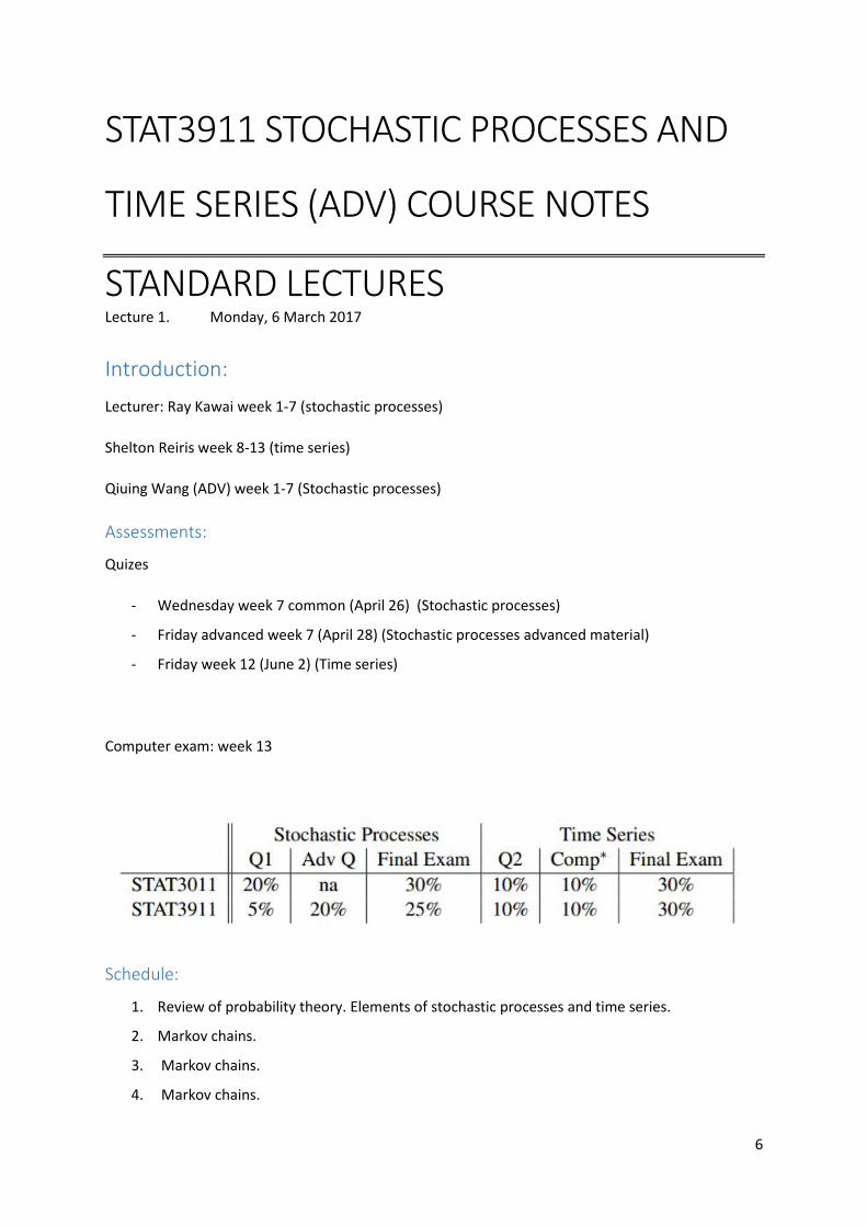
Assessments:
Quizes
- Wednesday week 7 common (April 26) (Stochastic processes)
- Friday advanced week 7 (April 28) (Stochastic processes advanced material)
- Friday week 12 (June 2) (Time series)
Computer exam: week 13
Schedule:
1. Review of probability theory. Elements of stochastic processes and time series.
2. Markov chains.
3. Markov chains.
4. Markov chains.

7
5. The Poisson process.
6. The Poisson process.
7. The Poisson process.
8. Time series data, components of a time series. Filtering to remove trends and seasonal
components.
9. Stationarity time series. Sample autocorrelations and partial autocorrelations. Probability
models for stationary time series. Moving Average (MA) models and properties.
10. Invertibility of MA models. Autoregressive (AR) models and their properties. Stationarity of
AR models. Mixed Autoregressive Moving Average (ARMA) models and their properties.
11. Homogeneous nonstationary time series (HNTS). Simple models for HNTS. Autoregressive
Integrated Moving Average (ARIMA) models and related results. Review of theoretical
patterns of ACF and PACF for AR, MA and ARMA processes. Identification of possible AR,
MA, ARMA and ARIMA models for a set of time series data.
12. Estimation and fitting ARIMA models via MM and MLE methods. Hypothesis testing,
diagnostic checking and goodness-of-fit tests. AIC for ARIMA models. Forecating methods for
ARIMA models.
13. Minimum mean square error (mmse) forecasting and its properties. Derivation of l-step
ahead mmse forecast function. Forecast updates. Forecast errors, related results and
applications.
Stochastic Processes:
In probability theory and related fields, a stochastic or random process is a mathematical
object usually defined as a collection of random variables. Historically, the random variables
were associated with or indexed by a set of numbers, usually viewed as points in time, giving the
interpretation of a stochastic process representing numerical values of some
system randomly changing over time, such as the growth of a bacterial population, an electrical
current fluctuating due to thermal noise, or the movement of a gas molecule.[1][4][5] Stochastic
processes are widely used as mathematical models of systems and phenomena that appear to
vary in a random manner. They have applications in many disciplines including sciences such
as biology,[6] chemistry,[7] ecology,[8] neuroscience,[9] and physics[10] as well
as technology and engineering fields such as image processing, signal processing,[11] information
theory,[12] computer science,[13] cryptography[14] and telecommunications.[15] Furthermore,

8
seemingly random changes in financial markets have motivated the extensive use of stochastic
processes in finance.[16][17][18]
Basic concenpts:
- Randomness, indexed by time
{𝑋𝑡: 𝑡 ∈ 𝕋}
Where 𝑡 ∈ [0, 𝑇] for some endtime 𝑡.
- Can be either discrete or continuous
State Time
Continuous Height,
temperature
Continuous
time
discrete Dice,
coinflip,
number of
people
1 day, 1
second, 1
year
Definition: Stochastic process
A stochastic process is a model of time-dependent random phenomena. A single random variable
describes a static random phenomena; a stochastic process is a collection of random variables
{𝑋𝑡: 𝑡 ∈ 𝕋}, one for each time 𝑡 ∈ 𝕋.
- Can be either discrete or continuous

9
Definition: Random walk
We have a time set 𝕋 and state space 𝑆. We defininte the stochastic process {𝑋𝑡: 𝑡 ∈ 𝕋}. In principle,
we need to know the joint distribution of (𝑋𝑡1 , 𝑋𝑡2 , … , 𝑋𝑡𝑛), where 𝑡𝑘 ∈ 𝕋, 𝑛 ∈ ℕ. This is difficult.
We define a random walk as a stochastic process {𝑋𝑡: 𝑡 ∈ 𝕋}, where 𝕋 = ℕ in such a way that
𝑋𝑡 = 𝑋𝑡−1 + 𝑍𝑡; (𝑡 ∈ 𝕋)
Where {𝑍𝑘}𝑘∈ℕ is a sequence of iid RV with ℙ(𝑍𝑘 = 1) = 𝑝, ℙ(𝑍𝑘 = −1) = 1 − 𝑝 for some 𝑝 ∈
(0,1).
The equation 𝑋𝑡 = 𝑋𝑡−1 + 𝑍𝑡 is an example of a difference equation. It is an implicit definition of 𝑋𝑡,
since it is only given in terms of 𝑋𝑡−1. In continuous time, this becomes the differential equation
Definition: Strong stationary
A SP {𝑋𝑡: 𝑡 ∈ 𝕋} is said to be strong stationary, if the two joint distributions of (𝑋𝑡1 , 𝑋𝑡2 , … , 𝑋𝑡𝑛) and
(𝑋𝑘+𝑡1 , 𝑋𝑘+𝑡2 , … , 𝑋𝑘+𝑡𝑛) are identical ∀𝑡1, … , 𝑡𝑛; 𝑘 + 𝑡1, … , 𝑘 + 𝑡𝑛 ∈ 𝕋
Definition: State space of stochastic process
The set of values that the 𝑋𝑡 ‘s can take is called the state space, 𝑆, of the stochastic process
Definition: Increments
An increment of a stochastic process is the amount by which its value changes over a period of time,
for example 𝑋𝑡𝑘+1 − 𝑋𝑡𝑘, where 𝑡𝑘 < 𝑡𝑘+1 ∈ 𝕋
Definition: Stationary increments
The SP {𝑋𝑡: 𝑡 ∈ 𝕋} is said to have stationary increments if the distribution of the increment depends
only on the difference between the two time points.
- If, for 𝑡1 ≤ 𝑡2 and 𝑡3 ≤ 𝑡4 ⟹ 𝑡2 − 𝑡1 = 𝑡4 − 𝑡3
𝑋𝑡2 − 𝑋𝑡1ℒ
=𝑋𝑡4 − 𝑋𝑡3
(the increments have the same distribution)
Eg: temperature between today and tomorrow is distributed the same

10
Example: stock prices
Let {𝑆𝑡: 𝑡 ∈ ℝ+} denote the price of one share of a specific stock. It might be considered reasonable
to assume that the distribution of the return over a period of duraction Δ > 0
𝑆𝑡+Δ − 𝑆𝑡𝑆𝑡
=𝑆𝑡+Δ𝑆𝑡
− 1
Depends on Δ but not 𝑡. Generally, we assume that {𝑆𝑡+Δ
𝑆𝑡: 𝑡 ∈ ℝ+} is a stationary stochastic process.
Accordingly, the log-price processes 𝑋 ≔ ln 𝑆𝑡 would have stationary increments 𝑋𝑡+Δ − 𝑋𝑡 =
ln (𝑆𝑡+Δ
𝑆𝑡), even though the stochastic process {𝑋𝑡: 𝑡 ∈ ℝ+} might not be stochastic. In other words,
for fixed Δ, the stochastic process 𝑌𝑡Δ ≔ 𝑋𝑡+Δ − 𝑋𝑡 is stationary.
Definition: Independent increments
A stochastic process {𝑋𝑡: 𝑡 ∈ 𝕋} has independent increments, if ∀𝑡 ∈ 𝕋, and Δ > 0|𝑡 + Δ ∈ 𝕋, the
increment 𝑋𝑡+Δ − 𝑋𝑡 is independent of all the past {𝑋𝑠: 𝑠 ∈ 𝕋} of the SP.
- The increments at some time period are independent of previous events.
o The first half of this course will assume stationary and independent increments
Markov Property:
In probability theory and related fields, a Markov process (or Markoff process), named after
the Russian mathematician Andrey Markov, is a stochastic process that satisfies the Markov
property[1][2] (sometimes characterized as "memorylessness"). Loosely speaking, a process
satisfies the Markov property if one can make predictions for the future of the process based

11
solely on its present state just as well as one could knowing the process's full history;
i.e., conditional on the present state of the system, its future and past states are independent.
A Markov chain is a type of Markov process that has either discrete state space or discrete
index set (often representing time), but the precise definition of a Markov chain varies.[3] For
example, it is common to define a Markov chain as a Markov process in either discrete or
continuous time with a countable state space (thus regardless of the nature of time)[4][5][6][7], but it is
also common to define a Markov chain as having discrete time in either countable or continuous
state space (thus regardless of the state space).[8]
- Future events only depend upon current time, and not previous events
Definition: Markov property
A SP {𝑋𝑡: 𝑡 ∈ 𝕋} is said to have a Markov Property if
𝑃(𝑋𝑡𝑚+1 ∈ 𝐴𝑚+1|𝑋𝑡1 ∈ 𝐴1, … , 𝑋𝑡𝑚 ∈ 𝐴𝑚) = 𝑃(𝑋𝑡𝑚+1 ∈ 𝐴𝑚+1|𝑋𝑡𝑚 ∈ 𝐴𝑚)
Where 0 ≤ 𝑡1 ≤ 𝑡2 ≤ ⋯ ≤ 𝑡𝑚 ≤ 𝑡𝑚+1 and {𝐴𝑘}(𝑘∈ℕ} is a sequence of measurable sets in 𝑆
Corollary: Independent increments have the Markov property
A SP {𝑋𝑡: 𝑡 ∈ 𝕋} with independent increments has the Markov property.
Example: State space of natural numbers
Eg, let 𝑆 = ℕ, then
𝑃(𝑋𝑡𝑚+1 = 𝑥𝑚+1|𝑋𝑡1 ∈ 𝐴1, … , 𝑋𝑡𝑚−1 ∈ 𝐴𝑚−1, 𝑋𝑡𝑚 = 𝑥𝑚)
= 𝑃(𝑋𝑡𝑚+1 − 𝑋𝑡𝑚 = 𝑥𝑚+1 − 𝑥𝑚|𝑋𝑡1 ∈ 𝐴1, … , 𝑋𝑡𝑚−1 ∈ 𝐴𝑚−1, 𝑋𝑡𝑚 = 𝑥𝑚)
= 𝑃(𝑋𝑡𝑚+1 − 𝑋𝑡𝑚 = 𝑥𝑚+1 − 𝑥𝑚|𝑋𝑡𝑚 = 𝑥𝑚) (𝑏𝑦 𝑖𝑛𝑑𝑒𝑝𝑒𝑛𝑑𝑒𝑛𝑡 𝑖𝑛𝑐𝑟𝑒𝑚𝑒𝑛𝑡𝑠)
= 𝑃(𝑋𝑡𝑚+1 = 𝑥𝑚+1|𝑋𝑡𝑚 = 𝑥𝑚)
Note, independent increments imply markov property, but not the reverse (as what if 𝑋𝑛+1 = 𝑋𝑛 +
𝜖𝑛, where 𝜖_𝑛|𝑥0, . . , 𝑥𝑛 ∼ 𝑁(−𝑋𝑛, 1) for example)?. This brings in the concept of filtration, where
we need to model the flow of public information.
Lecture 2. Tuesday, 7 March 2017
12
Definition: filtration
Let (Ω, ℱ) be a measureable space, and 𝕋 ⊆ [0,∞).
1. Assume ∀𝑡 ∈ 𝕋 ∃ 𝜎 −field, ℱ𝑡 ⊆ ℱ. Assume that, for 𝑠 ≤ 𝑡 ⟹ ℱ𝑠 ⊆ ℱ𝑡. We call the
collection of 𝜎 fields (𝐹𝑡)𝑡∈𝕋 a filtration.
2. A SP {𝑋𝑡: 𝑡 ∈ 𝕋} is said to be (ℱ)𝑡∈𝕋 adapted if, ∀𝑡 ∈ 𝕋, the RV 𝑋𝑡 is ℱ𝑡 − measurable.
Remark: filtration generated by a stochastic process and information
If the filtration (ℱ𝑡)𝑡∈𝕋 is generated by a stochastic process {𝑋𝑡: 𝑡 ∈ 𝕋}, then ∀𝑡 ∈ 𝕋
ℱ𝑡 = 𝜎(𝑋𝑠: 𝑠 ∈ 𝕋, 𝑠 ≤ 𝑡)
In this case, the 𝜎 −field ℱ𝑠 contains all the information of the SP up till time 𝑠.
- The concept of filtration can then generalise the definition of the Markov property
Definition: Markov Process
Let (Ω, ℱ, ℙ) be a probability space, and (ℱ𝑡)𝑡∈𝕋 be a filtration. A (ℱ𝑡)𝑡∈𝕋 adapted SP {𝑋𝑡: 𝑡 ∈ 𝕋} is
called a Markov process, if, ∀𝐵 ∈ 𝜎(𝑋𝑠: 𝑠 ≥ 𝑡)
ℙ(𝐵|ℱ𝑡) = ℙ(𝐵|𝑋𝑡)
(note that 𝐵 depends only on {𝑋𝑠: 𝑠 ≥ 𝑡}).
Lecture 3. Wednesday, 8 March 2017
Markov Chains
In probability theory and related fields, a Markov process (or Markoff process), named after
the Russian mathematician Andrey Markov, is a stochastic process that satisfies the Markov
property[1][2] (sometimes characterized as "memorylessness"). Loosely speaking, a process
satisfies the Markov property if one can make predictions for the future of the process based
solely on its present state just as well as one could knowing the process's full history;
i.e., conditional on the present state of the system, its future and past states are independent.
A Markov chain is a type of Markov process that has either discrete state space or discrete
index set (often representing time), but the precise definition of a Markov chain varies.[3] For
example, it is common to define a Markov chain as a Markov process in either discrete or
13
continuous time with a countable state space (thus regardless of the nature of time)[4][5][6][7], but it is
also common to define a Markov chain as having discrete time in either countable or continuous
state space (thus regardless of the state space).[8]
- Discrete time and discrete space problem
o After we will look at continuous time and discrete space (Poisson processes)
- That is to say, they are indexed by 𝑡 ∈ 𝕋 = ℕ = {0,1,2,… }
Basic concepts: Independence of increments are replaced by the Markov property
- That the future and the past are independent given the present
Notation: Given 𝑛, 𝑟, 𝑘0, … , 𝑘𝑛+𝑟, with 𝑃(𝑋𝑛 = 𝑘𝑛) > 0 :
- we write the past event as
{𝑋0 = 𝑘0, 𝑋1 = 𝑘1, … , 𝑋𝑛−1 = 𝑘𝑛−1} ≔ 𝐴
- And all future events as
{𝑋𝑛+1 = 𝑘𝑛+1, 𝑋𝑛+2 = 𝑘𝑛+2, … , 𝑋𝑛+𝑟 = 𝑘𝑛+1} ≔ 𝐵
We then get the conditional probability that:
𝑃(𝐴 ∩ 𝐵|𝑋𝑛 = 𝑘𝑛) = 𝑃(𝐴|𝑋𝑛 = 𝑘𝑛)𝑃(𝐵|𝑋𝑛 = 𝑘𝑛)
- This is equivalent that ∀𝑛 ∈ ℕ, 𝑘0, 𝑘1, … , 𝑘𝑛+1 with 𝑃(𝑋0 = 𝑘0, 𝑋1 = 𝑘1, … , 𝑋𝑛−1 = 𝑘𝑛−1) >
0 that:
𝑃(𝑋𝑛+1 = 𝑘𝑛+1|𝑋0 = 𝑘0, … , 𝑋𝑛 = 𝑘𝑛) = 𝑃(𝑋𝑛+1 = 𝑘𝑛+1|𝑋𝑛 = 𝑘𝑛)
(by the Markov property)
Transiontion probability
The right hand side of the above equation is known as the transition probability. It does not depend
on time, but only on the states 𝑘𝑛 and 𝑘𝑛+1. We write that
𝑃(𝑋𝑛+1 = 𝑗 |𝑋𝑛 = 𝑘) ≔ 𝑝𝑘,𝑗
Gambler ruin problem:
- Start with an amount of money $𝑛, with probability 𝑝 you win $1, and 𝑞 = 1 − 𝑝 you lose
$1. You stop after you either:
o Lose all money
o Win up to a certain amount $𝑁
14
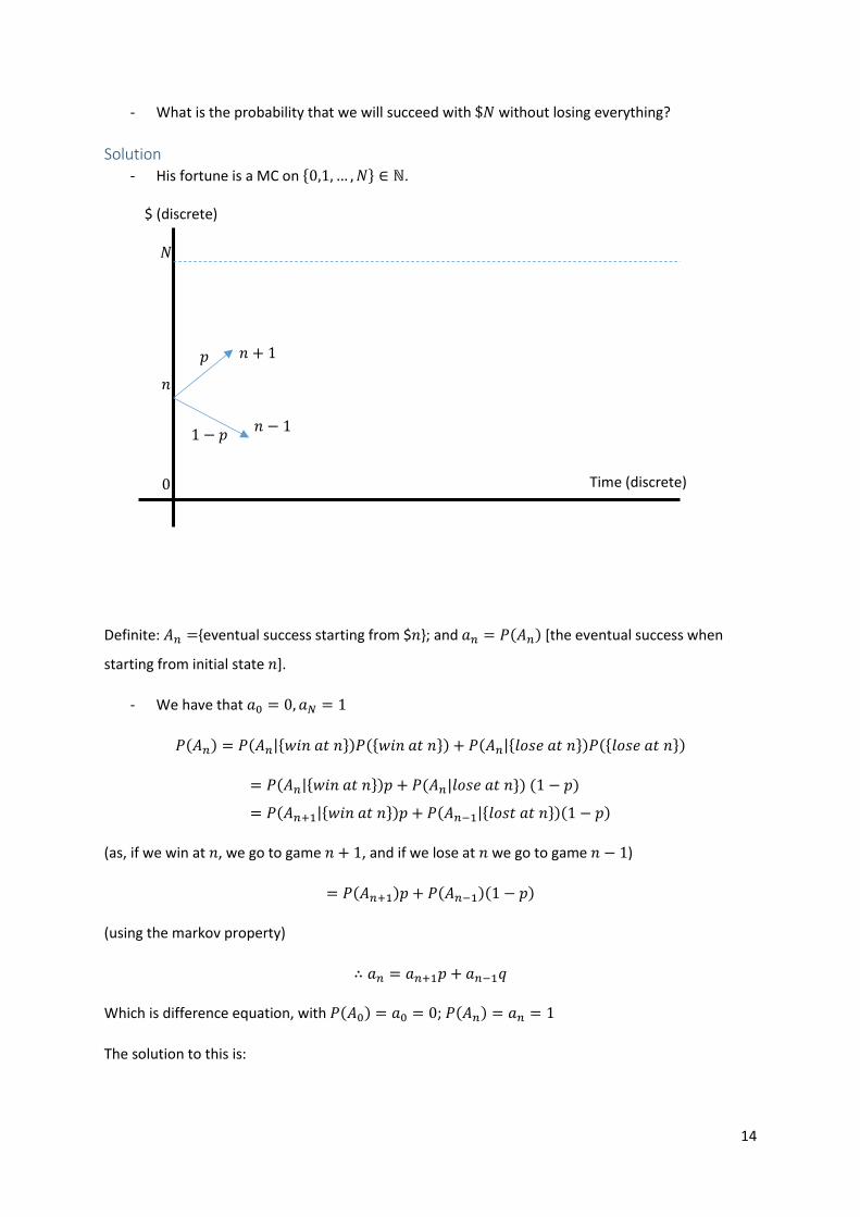
- What is the probability that we will succeed with $𝑁 without losing everything?
Solution - His fortune is a MC on {0,1,… ,𝑁} ∈ ℕ.
Definite: 𝐴𝑛 ={eventual success starting from $𝑛}; and 𝑎𝑛 = 𝑃(𝐴𝑛) [the eventual success when
starting from initial state 𝑛].
- We have that 𝑎0 = 0, 𝑎𝑁 = 1
𝑃(𝐴𝑛) = 𝑃(𝐴𝑛|{𝑤𝑖𝑛 𝑎𝑡 𝑛})𝑃({𝑤𝑖𝑛 𝑎𝑡 𝑛}) + 𝑃(𝐴𝑛|{𝑙𝑜𝑠𝑒 𝑎𝑡 𝑛})𝑃({𝑙𝑜𝑠𝑒 𝑎𝑡 𝑛})
= 𝑃(𝐴𝑛|{𝑤𝑖𝑛 𝑎𝑡 𝑛})𝑝 + 𝑃(𝐴𝑛|𝑙𝑜𝑠𝑒 𝑎𝑡 𝑛}) (1 − 𝑝)
= 𝑃(𝐴𝑛+1|{𝑤𝑖𝑛 𝑎𝑡 𝑛})𝑝 + 𝑃(𝐴𝑛−1|{𝑙𝑜𝑠𝑡 𝑎𝑡 𝑛})(1 − 𝑝)
(as, if we win at 𝑛, we go to game 𝑛 + 1, and if we lose at 𝑛 we go to game 𝑛 − 1)
= 𝑃(𝐴𝑛+1)𝑝 + 𝑃(𝐴𝑛−1)(1 − 𝑝)
(using the markov property)
∴ 𝑎𝑛 = 𝑎𝑛+1𝑝 + 𝑎𝑛−1𝑞
Which is difference equation, with 𝑃(𝐴0) = 𝑎0 = 0; 𝑃(𝐴𝑛) = 𝑎𝑛 = 1
The solution to this is:
𝑁
𝑛
0
𝑝
1 − 𝑝
𝑛 + 1
𝑛 − 1
$ (discrete)
Time (discrete)

15
𝑎𝑛 =
{
1 − (
1 − 𝑝𝑝 )
𝑛
1 − (1 − 𝑝𝑝
)𝑁 ; 𝑖𝑓 𝑝 ≠
1
2
𝑛
𝑁; 𝑖𝑓 𝑝 =
1
2
- Note that this expression is continuous in 𝑝; and that the 𝑛
𝑁 expression can be derived based
on the one for 𝑝 ≠1
2 using the asymptotic behavious 1 − (
𝑞
𝑝)𝑛= 4𝑛 (𝑝 −
1
2) +
𝑂 ((𝑝 −1
2)2) as 𝑝 →
1
2.
We get the same solution if we let 𝛽𝑛 be the probability of eventual ruin when starting at 𝑛, finding
that 𝛽𝑛 = 𝑝𝛽𝑛+1 + 𝑞𝛽𝑛−1, with 𝛽0 = 1 and 𝛽𝑁 = 0. This means that the gambler must either
succed or be ruined, and the gambler will not be able to converge to a steady state of some other
amount of money.
Also; observe that in the limit:
lim𝑁↑+∞
𝑎𝑛 =
{
1 − (𝑞
𝑝)𝑛
[> 0]; 𝑖𝑓 𝑝 >1
2
0; 𝑝 ≤1
2
So, taking 𝑁 ↑ +∞ means that in the limit, the gambler will only ever stop if ruined. In this situation,
if each gamble is in the player’s favour (𝑝 >1
2), then there is a positive probability that the gambler
will never get ruined, but instead become infinitely rich. If each gamble is out of favour, (𝑝 <1
2),
then the gambler will get ruined almost surely.
Classification of states:
𝑛 step transition probability notation: Let
𝑝𝑘0,𝑘𝑛(𝑛) ≔ ℙ𝑘0(𝑋𝑛 = 𝑘𝑛) = ℙ(𝑋𝑛 = 𝑘𝑛|𝑋0 = 𝑘0)
- The probability that we are at state 𝑘𝑛, given that we started at 𝑘0 𝑛 steps ago.
- For ease of notation, 𝑝𝑖,𝑗(1) = 𝑝𝑖,𝑗
16
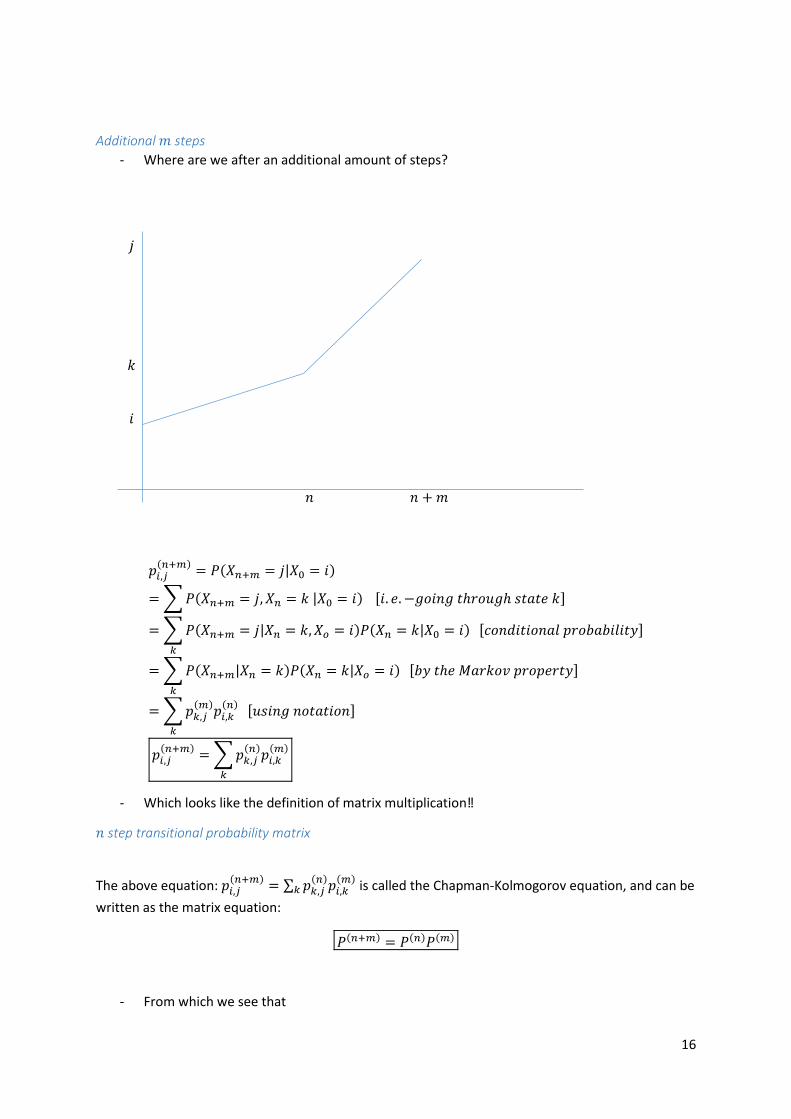
Additional 𝑚 steps
- Where are we after an additional amount of steps?
𝑝𝑖,𝑗(𝑛+𝑚) = 𝑃(𝑋𝑛+𝑚 = 𝑗|𝑋0 = 𝑖)
=∑𝑃(𝑋𝑛+𝑚 = 𝑗, 𝑋𝑛 = 𝑘 |𝑋0 = 𝑖) [𝑖. 𝑒. −𝑔𝑜𝑖𝑛𝑔 𝑡ℎ𝑟𝑜𝑢𝑔ℎ 𝑠𝑡𝑎𝑡𝑒 𝑘]
=∑𝑃(𝑋𝑛+𝑚 = 𝑗|𝑋𝑛 = 𝑘, 𝑋𝑜 = 𝑖)𝑃(𝑋𝑛 = 𝑘|𝑋0 = 𝑖)
𝑘
[𝑐𝑜𝑛𝑑𝑖𝑡𝑖𝑜𝑛𝑎𝑙 𝑝𝑟𝑜𝑏𝑎𝑏𝑖𝑙𝑖𝑡𝑦]
=∑𝑃(𝑋𝑛+𝑚|𝑋𝑛 = 𝑘)𝑃(𝑋𝑛 = 𝑘|𝑋𝑜 = 𝑖)
𝑘
[𝑏𝑦 𝑡ℎ𝑒 𝑀𝑎𝑟𝑘𝑜𝑣 𝑝𝑟𝑜𝑝𝑒𝑟𝑡𝑦]
=∑𝑝𝑘,𝑗(𝑚)𝑝𝑖,𝑘
(𝑛)
𝑘
[𝑢𝑠𝑖𝑛𝑔 𝑛𝑜𝑡𝑎𝑡𝑖𝑜𝑛]
𝑝𝑖,𝑗(𝑛+𝑚) =∑𝑝𝑘,𝑗
(𝑛)𝑝𝑖,𝑘(𝑚)
𝑘
- Which looks like the definition of matrix multiplication‼
𝑛 step transitional probability matrix
The above equation: 𝑝𝑖,𝑗(𝑛+𝑚) = ∑ 𝑝𝑘,𝑗
(𝑛)𝑝𝑖,𝑘(𝑚)
𝑘 is called the Chapman-Kolmogorov equation, and can be
written as the matrix equation:
𝑃(𝑛+𝑚) = 𝑃(𝑛)𝑃(𝑚)
- From which we see that
𝑖
𝑘
𝑗
𝑛 𝑛 +𝑚

17
𝑃(𝑛) = (𝑃(1))𝑛
In the matrix:
𝑜𝑟𝑖𝑔𝑖𝑛
𝐷𝑒𝑠𝑖𝑛𝑎𝑡𝑖𝑜𝑛
( )
Accessibility:
We say that state 𝑗 is accessible from state 𝑖, ∃ some number of steps 𝑛 ∈ ℕ+ |𝑝𝑖,𝑗(𝑛)
> 0
- i.e.: it is possible to get to state 𝑗 from state 𝑖 after some amount of states (as probability >
0)
- can write as 𝑖 → 𝑗
Communicate
If 𝑖 and 𝑗 are accessible from one another, they are said to communicate, written as 𝑖 ↔ 𝑗
Properties of communicating states:
1. reflexivity: 𝑖 ↔ 𝑖
2. symmetry: 𝑖 ↔ 𝑗 ⟺ 𝑗 ↔ 𝑖
3. transitivity: if 𝑖 ↔ 𝑗, and 𝑗 ↔ 𝑘; then 𝑖 ↔ 𝑘
Communicating classes:
Communicating states can be partitioned into communicating classes:
- largest set A of states such that all 𝑖, 𝑗 ∈ 𝐴 communicate.
- all states in a communicating class communicate with one another
o in the gamblers ruin problem; there are 3 communicating classes:
{𝑁}
{0}
{1,2,… ,𝑁 − 1}
Closed communicating classes
We say a communicating class 𝐶 is closed if no state outside of 𝐶 can be reached from any state in
𝐶.
i.e:
𝑝𝑖,𝑗 = 0 for 𝑖 ∈ 𝐶 and 𝑗 ∉ 𝐶
Irreducible:
If the markov chain consists of only 1 communicating class, then the MC is said to be irreducible.
Absorbing state
A state is said to be absorbing, if we cannot go anywhere after it.
- i.e; the set {𝑗} is a closed class, that is 𝑝𝑗,𝑗 = 1

18
o in the gambler’s guin problem: 𝑝0,0 = 1 and 𝑝𝑁,𝑁 = 1
Lecture 4. Monday, 13 March 2017
Example: Markov Chain
Consider the MC with states {1,2,3}
𝑃 =
(
1
2
1
20
1
2
1
4
1
4
01
3
2
3)
Eg: (probability of 1 → 3 is 0)
Accessible states:1,1; 1,2; 2,1; 2,2; 2,3; 3,2; 3,3
1 ↔ 2 ↔ 3
{1,2,3} is a communicating class
Example 2: markov chain
4 states with
𝑃 =
(
1
2
1
20 0
1
2
1
20 0
1
4
1
4
1
4
1
40 0 0 1)
4 is absorbing sate
1 and 2 communicate
1,2,3,4 is accessible from 3.
- This is not irreducible (3 communicating classes)
Example 3: weather
Probability of fine or rain (0,1). Chances of rain tomorrow depends on today’s conditions. If it is fine
today, probability of fine tomorrow is 0.7. if it is rainy today, probability of fine tomorrow is 0.4
𝑃 = (0.7 0.3. 4 0.6
)
- This is irreducible
3 step transition:
𝑃3 = (0.7 0.3. 4 0.6
)3
= (0.583 . 417. 556 . 441
)

19
Ie: 𝑝0,1(3)= 0.417
Recurrence and transience
Let 𝑓𝑖,𝑗(𝑛)
denote the probability that the first transition into 𝑗 takes place at time 𝑛, when the chain
starts at state 𝑖
𝑓𝑖,𝑗(𝑛) ≔ ℙ({𝑋𝑛 = 𝑗} ∩ {𝑋𝑛−1, 𝑋𝑁−2, … , 𝑋1 ≠ 𝑗})
- i.e. the “first” probability from 𝑖 → 𝑗 after 𝑛 steps, without having vistited 𝑗 in between.
- If 𝑓𝑖,𝑗(0)= 0 if 𝑖 ≠ 𝑗 and 𝑓𝑖,𝑗
(0)= 1 if 𝑖 = 𝑗. Then the quantity becomes:
𝑓𝑖,𝑗 ≔∑𝑓𝑖,𝑗(𝑛)
+∞
𝑛=1
= ℙ(𝑋𝑛 = 𝑗 for some 𝑛 ≥ 1|𝑋0 = 1)
Recurrence definition: Indicates the probability of ever making a transition into state 𝑗 when the chain starts at 𝑖. We call
state 𝑗 recurrent if 𝑓𝑗,𝑗 = 1 (i.e.: starting at 𝑗, the chain will almost surely return to itself in a finite
number of steps).
Transient definition: A non recurrent state is said to be transient.
- For example, if 𝑓𝑗,𝑗 < 1, then state 𝑗 is transient
- Not sure that we will return
Green Function: The Green function of the MC is the expected number of visits to 𝑗 for the chain starting at 𝑖.
𝐺(𝑖, 𝑗) ≔ ∑𝑝𝑖,𝑗(𝑛)
+∞
𝑛=0
= ∑𝔼(𝕀(𝑋𝑛 = 𝑗)|𝑋0 = 𝑖)
+∞
𝑛=0
= 𝔼∑(𝕀(𝑋𝑛 = 𝑗)|𝑋0 = 𝑖)
+∞
𝑛=0
- Is the expected number of visits to 𝑗 starting from state 𝑖.
Transience and green function:
State 𝑗 is transient iff 𝐺(𝑖, 𝑗) < ∞ (i.e. the expected number of moves before returning is finite)
𝑡𝑟𝑎𝑛𝑠𝑖𝑒𝑛𝑐𝑒 ⟺ 𝐺(𝑗, 𝑗) < ∞

20
Proof:
After visiting 𝑗, the probability of returning is 𝑓𝑗,𝑗 after some time. This happens every time we return
to state 𝑗. As we are counting the number of successes of visits to 𝑗, this means the distribution is
geometric; with 𝑝 = 𝑓𝑗,𝑗. ∼ 𝐺𝑒𝑜𝑚𝑒𝑡𝑟𝑖𝑐(𝑓𝑗,𝑗)
Mean of geometric is 𝑝
1−𝑝
𝐸[𝑋] =𝑓𝑗,𝑗
1 − 𝑓𝑗,𝑗
But we already know that 𝐺(𝑗, 𝑗) = 𝐸(𝑋), so
𝑓𝑘,𝑘 < 1 iff 𝐺(𝑗, 𝑗) < ∞
Lecture 5. Tuesday, 14 March 2017
Recurrence of communicating states
If 𝑖 ↔ 𝑗 and if state 𝑖 is recurrent, then state 𝑗 is recurrent.
Proof:
As 𝑖 ↔ 𝑗∃𝑚, 𝑛|𝑝𝑖,𝑗𝑚 , 𝑝𝑖,𝑗
𝑛 > 0. We fix such 𝑚, 𝑛, it then holds that ∀𝑠 ≥ 0
𝑝𝑗,𝑗𝑛+𝑠+𝑚 ≥ 𝑝𝑗,𝑖
𝑛 𝑝𝑖 , 𝑖𝑠𝑝𝑖, 𝑗
𝑚
Due to the chapman kolmorgov equation when:
∑𝑝𝑗,𝑗𝑛+𝑠+𝑚
𝑠
≥∑𝑝𝑗,𝑖𝑛 𝑝𝑖,𝑖
𝑠 𝑝𝑖,𝑗𝑚
𝑠
= 𝑝𝑗,𝑖𝑛 𝑝𝑖,𝑗
𝑚∑𝑝𝑖,𝑖𝑠
𝑠
= 𝑝𝑗,𝑖𝑛 𝑝𝑖,𝑗
𝑚𝐺(𝑖, 𝑖) = ∞
Recurrence and accessibility
If state 𝑖 is recurrent and state 𝑗 is accessible from 𝑖, then 𝑓𝑖,𝑗 = 1 and 𝑖 ↔ 𝑗
Proof:
Let 𝑋0 = 𝑖. As 𝑗 is accessible from 𝑖∃𝑛|𝑝𝑖,(𝑛) > 0. Fix such 𝑛, we define the following:
𝐴0 = {𝑋𝑛 = 𝑗}; 𝑇1 = min{𝑘 ≥ 𝑛:𝑋𝑘 = 𝑖}
𝐴1 = {𝑋𝑇1+𝑛 = 𝑗}; 𝑇2 = min{𝑘 ≥ 𝑇1 + 𝑛:𝑋𝑘 = 𝑖}
…
𝐴𝑟 = {𝑋𝑇𝑟+𝑛 = 𝑗}; 𝑇𝑟+1 = min{𝑘 ≥ 𝑇𝑟 + 𝑛: 𝑋𝑘 = 𝑖}
time
j j

21
Since 𝑖 is recurrent; 𝑇𝑘 are finite. Then, the MC {𝐴𝑛} are independent and have th 𝑝𝑖,𝑗𝑛 so one of
them occurs.
Remark:
- We have used the Strong Markov Property to show this. Which always holds for discrete
time markov chains, and usually for continuous ones. It says that: if 𝑁 is the stopping time of
a MC {𝑋𝑛}𝑛∈ℕ+ and we write 𝜓(𝑖, 𝐵) = 𝑃𝑖((𝑋0, 𝑋1, … ) ∈ 𝐵)
The Strong markov property says that:
𝑃((𝑋𝑁 , 𝑋𝑁+1, … ) ∈ 𝐵|𝑋0, 𝑋1, … , 𝑋𝑁) = 𝜓(𝑋𝑁 , 𝐵)
Example:
Consider the 4 staes with probability:
𝑃 =
(
0 0
1
2
1
21 0 0 00 1 0 00 0 0 0)
It is easy to see that all states communicate: 1 → 3 → 2 → 1 → 4 → 2 → 1
- All states must be recurrent (using the above property)
Example 2:
𝑃 =
(
1
2
1
20 0 0
1
2
1
20 0 0
0 01
2
1
20
0 01
2
1
20
1
4
1
40 0
1
2)
The chain consists of 3 classes: {1,2}, {3,4}, {5}.

22
The first two classes are recurrent, if the chin starts at 1 it will come back to 1 sometime a.s. however;
if it starts at 5, it may never come back, as if it goes to state {1,2} it can never return.
Period:
Definition
The period of state 𝑘 is the greatest common divisor of the number of steps to come back to 𝑖,
starting from 𝑖 {𝑛 ∈ ℕ: 𝑝𝑘,𝑘(𝑛) > 0}, often written as
𝑑(𝑘)
If 𝑑(𝑘) = 1 then the state is called aperiodic.
Lecture 6. Wednesday, 15 March 2017
Remark on periodicity:
The minimum number of steps required to return is purely irrelevant to the concept of periodicity,
eg: consider
𝑃 = (0
1
20
0 0 11 0 0
)
Observe that: starting from state 2; the chain returns to state 2 after 3,5,6 steps. The minimum
number of steps required to return to state 2 startin at 2 is 3. Nevertheless, the greatest common
divisor is 1, so the periodicity is 1.
Communicating states and periodicity
If 𝑖 ↔ 𝑗 then 𝑑(𝑖) = 𝑑(𝑗)
Proof:
If 𝑖 = 𝑗, result is trivial. Suppose 𝑖 ≠ 𝑗. We show that𝑖 ↔ 𝑗 means 𝑑(𝑖) divides 𝑑(𝑗). Find a positive
interer 𝑠, such that 𝑝𝑖,𝑖𝑠 > 0. By definition, this integer divides 𝑑(𝑖). Moreover, there exists positive
interges 𝑚, 𝑛|𝑝𝑖,𝑗𝑛 , 𝑝𝑗,𝑖
𝑛 > 0. Then we have that:
𝑝𝑗,𝑗𝑛+𝑚 ≥ 𝑝𝑗,𝑖
𝑛 𝑝𝑖,𝑗𝑚 > 0
So (𝑛 + 𝑚) divides 𝑑(𝑗). By visiting 𝑖 in the middle, we have:
𝑝𝑗,𝑗𝑛+𝑠+𝑚 ≥ 𝑝𝑗,𝑖
𝑛 𝑝𝑖,𝑖𝑠 𝑝𝑖,ℎ
𝑚 > 0
So (𝑛 + 𝑠 +𝑚) divides 𝑑(𝑗). ∴ 𝑠 divides 𝑑(𝑗) and 𝑑(𝑖). Meaning that 𝑑(𝑖) = 𝑑(𝑗) as they are the
greatest common divisor
23
Example: Random walk:
Consider the MC on ℤ such that, for a given 𝑝 ∈ [0,1]; 𝑘 ∈ ℤ
𝑝𝑘,𝑘+1 = 𝑝; 𝑝𝑘,𝑘−1 = 1 − 𝑝
(example of a MC with period 2).
We show that, for 𝑝 =1
2 it is recurrent. First, observe that the n step transition probability is
binomial
𝑝0,0(2𝑛)
= (2𝑛𝑛) (1
2)𝑛
(1
2)𝑛
Which we approximiate (using Stirlings approximation), as
𝑝0,0(2𝑛)
∼1
√𝜋𝑛
Hence, 𝐺(0,0) = ∞.
- One of a famous theorems in probability extends to higher dimensions (Polya theorem),
which says symmetric random walks on ℤ𝑘 are transient iff 𝑘 ≥ 3
- Computing the probability of this for a 1D random walk will ever return if 𝑝 ≠1
2: WLOF,
suppose we start at 0. Let 𝑌𝑘 be the 𝑘𝑡ℎ step of the walk, {𝑌𝑘}𝑘∈ℕ is a sequence of iid RV
with
𝑌𝑘 = {+1; 𝑝𝑟𝑜𝑏𝑎𝑏𝑖𝑙𝑖𝑡𝑦 𝑝
−1; 𝑝𝑟𝑜𝑏𝑎𝑏𝑖𝑙𝑖𝑡𝑦 1 − 𝑝
𝑋𝑛 denotes the position of the walk after 𝑛 steps, with 𝑋0 = 0. So 𝑋𝑛 = ∑ 𝑌𝑘𝑛𝑘−1 .
Considering the first transition,
𝑃(𝑒𝑣𝑒𝑟 𝑟𝑒𝑡𝑢𝑟𝑛|𝑋0 = 0)
= 𝑃(𝑒𝑣𝑒𝑟 𝑟𝑒𝑡𝑢𝑟𝑛|𝑋0 = 0, 𝑌1 = 1)𝑃(𝑌1 = 1)
+ 𝑃(𝑒𝑣𝑒𝑟 𝑟𝑒𝑡𝑢𝑟𝑛|𝑋0 = 0, 𝑌1 = −1)𝑃(𝑌1 = −1)
= 𝑃(𝑒𝑣𝑒𝑟 𝑟𝑒𝑡𝑢𝑟𝑛|𝑋0 = 0, 𝑌1 = 1)𝑝 + 𝑃(𝑒𝑣𝑒𝑟 𝑟𝑒𝑡𝑢𝑟𝑛|𝑋0 = 0, 𝑌1 = −1)(1 − 𝑝)
If 𝑝 >1
2, (walk tends in positive direction), observe by the law of large numbers that as 𝑛 ↑
+∞
1
𝑛∑𝑌𝑘
𝑛
𝑘=1
→ 𝐸(𝑌1) = 2𝑝 − 1 (> 0)𝑎. 𝑠.
Which implies that ∑ 𝑌𝑘𝑛𝑘−1 tends to infinity almost surely. If we investigate the transitional
probability 𝑃(𝑒𝑣𝑒𝑟 𝑟𝑒𝑡𝑢𝑟𝑛|𝑋0 = 0, 𝑌1 = +1) conditioning on the second transition, we get
24
= 𝑃(𝑒𝑣𝑒𝑟 𝑟𝑒𝑡𝑢𝑟𝑛|𝑋0 = 0, 𝑌1 = +1,𝑌2 = −1)𝑃(𝑌2 = −1)
+ 𝑃(𝑒𝑣𝑒𝑟 𝑟𝑒𝑡𝑢𝑟𝑛|𝑋0 = 0, 𝑌1 = +1,𝑌2 = +1)𝑃(𝑌2 = +1)
= 𝑃(𝑒𝑣𝑒𝑟 𝑟𝑒𝑡𝑢𝑟𝑛|𝑋0 = 0, 𝑌1 = 1, 𝑌1 = −1)(1 − 𝑝) + 𝑃(𝑒𝑣𝑒𝑟 𝑟𝑒𝑡𝑢𝑟𝑛|𝑋0 = 0, 𝑌1 = 1, 𝑌2 = 1)𝑝
= 1 − 𝑝 + 𝑃(𝑒𝑣𝑒𝑟 𝑟𝑒𝑡𝑢𝑟𝑛|𝑋0 = 0, 𝑌1 = +1,𝑌2 = +1)𝑝
= 1 − 𝑝 + 𝑃(𝑒𝑣𝑒𝑟 𝑒𝑛𝑡𝑒𝑟 0|𝑋0 = 0, 𝑋1 = 1, 𝑋2 = 2)𝑝
Which holds as the walk restrats after 2 steps. If the walk is at state 𝑋2 = 2, in order to ever return
to state 0, we must first ever enter state 1. The probability that the walk ever enters state 1 starting
from 2 is identical to 𝑃(𝑒𝑣𝑒𝑟 𝑟𝑒𝑡𝑢𝑟𝑛 𝑡𝑜 0|𝑋1 = 1). Similary, the probability that the walk ever
enters state 0 from 1 is 𝑃(𝑒𝑣𝑒𝑟 𝑟𝑒𝑡𝑢𝑟𝑛 𝑡𝑜 0|𝑋1 = 1). And so:
𝑃(𝑒𝑣𝑒𝑟 𝑒𝑛𝑡𝑒𝑟 0|𝑋2 = 2)
= 𝑃(𝑒𝑣𝑒𝑟 𝑒𝑛𝑡𝑒𝑟 0|𝑒𝑣𝑒𝑟 𝑒𝑛𝑡𝑒𝑟 1 𝑠𝑡𝑎𝑟𝑡𝑖𝑛𝑔 𝑓𝑟𝑜𝑚 2)𝑃(𝑒𝑣𝑒𝑟 𝑒𝑛𝑡𝑒𝑟 1|𝑠𝑡𝑎𝑟𝑡𝑖𝑛𝑔 𝑓𝑟𝑜𝑚 2)
+ 𝑃(𝑒𝑣𝑒𝑟 𝑒𝑛𝑡𝑒𝑟 0|𝑛𝑒𝑣𝑒𝑟 𝑒𝑛𝑡𝑒𝑟 1 𝑠𝑡𝑎𝑟𝑡𝑖𝑛𝑔 𝑓𝑟𝑜𝑚 2)𝑃(𝑛𝑒𝑣𝑒𝑟 𝑒𝑛𝑡𝑒𝑟 1|𝑠𝑡𝑎𝑟𝑡𝑖𝑛𝑔 𝑓𝑟𝑜𝑚 2)
= 𝑃(𝑒𝑣𝑒𝑟 𝑒𝑛𝑡𝑒𝑟 0|𝑠𝑡𝑎𝑟𝑡 𝑓𝑟𝑜𝑚 1)𝑃(𝑒𝑣𝑒𝑟 𝑒𝑛𝑡𝑒𝑟 1|𝑠𝑡𝑎𝑟𝑡 𝑓𝑟𝑜𝑚 2)
= 𝑃(𝑒𝑣𝑒𝑟 𝑒𝑛𝑡𝑒𝑟 0|𝑠𝑡𝑎𝑟𝑡 𝑓𝑟𝑜𝑚 1)2
We get that: 𝑃(𝑒𝑣𝑒𝑟 𝑟𝑒𝑡𝑢𝑟𝑛|𝑋0 = 0, 𝑌1 = +1) = 1 − 𝑝 + 𝑝𝑃(𝑒𝑣𝑒𝑟 𝑟𝑒𝑡𝑢𝑟𝑛|𝑋0 = 0, 𝑌1 = +1)2
Givins us:
𝑃(𝑒𝑣𝑒𝑟 𝑟𝑒𝑡𝑢𝑟𝑛|𝑋0 = 0, 𝑌1 = +1) = 1 𝑜𝑟1 − 𝑝
𝑝
The probability =1 is impossible, as we know by transience that it is strictly less than 1. Giving us that
𝑃(𝑒𝑣𝑒𝑟 𝑟𝑒𝑡𝑢𝑟𝑛|𝑋0 = 0, 𝑌1 = +1) =1 − 𝑝
𝑝
∴ 𝑃(𝐸𝑣𝑒𝑟 𝑟𝑒𝑡𝑢𝑟𝑛) =2
1 − 𝑝
For 𝑝 <1
2, we get 𝑃(𝑒𝑣𝑒𝑟 𝑟𝑒𝑡𝑢𝑟𝑛_ = 2𝑝
Generally thr probability of returning in a Random Walk is:
𝑃(𝑒𝑣𝑒𝑟 𝑟𝑒𝑡𝑢𝑟𝑛) = 2min{𝑝, 1 − 𝑝}
For example, if 𝑝𝑘,𝑘+1 =2
3; 𝑝𝑘,𝑘−1 =
1
3, starting at 0, the walk will come back to 0 again with
probability 2
3. (note the above result inclues 𝑝 =
1
2→ 𝑃(𝑒𝑣𝑒𝑟 𝑟𝑒𝑡𝑢𝑟𝑛) = 1
Recommended