Stackelberg versus Cournot Oligopoly withPrivate Information
Eray Cumbul∗†
IESE Business School, Barcelona
Abstract
In this paper, we compare an n-firm Cournot game with a Stackelbergmodel, where n-firms choose outputs sequentially, in a stochastic demandenvironment with private information. The Stackelberg perfect revealingequilibrium expected output and total surplus are lower while expectedprice and total profits are higher than the Cournot equilibrium ones irre-spective of how noisy both the demand shocks and private demand signalsof firms are. These rankings are the opposite to the rankings of prices, to-tal output, surplus, and profits under perfect information. Our Stackelbergmodel identifies the presence of four effects, which are absent under theCournot model. Because of i) the signaling effect, early-mover firms wouldlike to set low quantities to signal to their followers that the demand is low.This effect reduces ii) first-mover advantages. Moreover, as followers inferthe signals of their predecessors, they are better informed about demandcompared to Cournot oligopolists. But this iii) information acquisition offollowers also imposes iv) negative externalities on their rivals as rivals haveless value from exploiting their demand information. Only i) and iv) favorCournot over Stackelberg in welfare terms and they are the dominant ones.We also study a number of implications of our results in examining therelationships of prices, profits, and welfare with market concentration.
∗[email protected], This version: February 27, 2014†I am deeply grateful to Gabor Virag for his guidance and patience. I would like to thank
seminar participants at the IESE Business School, Bilkent University, TOBB University ofEconomics and Technology, ADA university, Antalya International University, University ofRochester, University of Toronto St. George, and University of Toronto Mississauga. I alsothank Paulo Barelli, Andrew F. Daughety, Alberto Galasso, Srihari Govindan, Asen Kochov,Semih Koray, Martin Osborne, Morten Olsen, Ayca Ozdogan, Roman Pancs, Carolyn Pitchik,Michael Raith, William Thomson, Mihkel M. Tombak, Xavier Vives, and Kemal Yildiz for theiruseful comments and suggestions. I thank Tubitak for their financial support. Of course, allerrors are mine.
1 Introduction
The Stackelberg- and the Cournot models are two of the leading frameworks in
which economists have studied oligopolistic competition. Among others, Anderson
and Engers (1992) have argued that the simultaneous-move Cournot model is
applicable to characterize an industry where lags in the observation of output
decisions are long, whereas the sequential-move Stackelberg model applies when
the reverse holds. While many industries fit the Cournot framework better1,
Shinkai (2000) has argued that the DRAM market (i.e., the market for the main
memory component of most computers and many electronic systems) is better
described by the Stackelberg model because firms make sequential capacity choices
in an irreversible manner.2
It is important to understand how the implications of the two models dif-
fer with respect to total output, welfare and producer surplus for at least three
reasons. First, such an understanding provides insights into the mechanics of
those important theoretical models. Relatedly, it also helps us in deciding which
framework (if either) is more appropriate for studying a given industry given the
observed price and output levels. Second, once it has been decided which model
fits a given industry better, the policy maker can assess better whether mergers or
other industry developments may help or hurt consumers. The answer may very
well depend on which model one thinks is more appropriate to describe an in-
dustry. Third, comparing these models also have implications on the relationship
between market concentration and welfare, which is affected by the asymmetries
among firms. When all firms are identical except for the timing of production (as
in our model), the Stackelberg model yields a higher HHI (Herfindahl-Hirschman
Index), which indicates a higher degree of concentration of the market, than does
the Cournot model.3 Hence total welfare comparison between these models helps
us understand whether concentration is beneficial or not for the society.
1For instance, Lopex et al. (2002) show that the Cournot competition is widespread in 32US food processing industries over the 1972-1992 period.
2Kadiyali et al. (2001) point out three structural new empirical industrial organization(NEIO) approaches that can identify competitive interactions among firms (e.g., Cournot orStackelberg) in a given industry. These approaches are 1) The menu approach, 2) The conjecturalvariations (CV) approach, and 3) The conduct parameter and the weighted profit approaches.
3Besides firm asymmetries, there are other factors that can affect the degree of market con-centration, e.g., the number of firms in the market. However, those factors are not in the scopeof this paper.
1
Unfortunately, the current literature compares the Stackelberg and Cournot
equilibrium outcomes under the assumption that the demand is known.4 An
important lesson learned is that total output and welfare under the Stackelberg
competition are greater than or equal to the ones under the Cournot competition
when the demand is known by the firms and costs are symmetric and linear. In
a leader-follower game with perfect information, the leader typically produces a
larger quantity and makes larger profits whereas the follower produces a lower
quantity and makes lower profits than in a simultaneous-move game. Strategic
substitutability among firm quantity decisions is the main driving force behind this
result. Therefore, as we move from simultaneous-move games to sequential-move
ones, this reallocation of firms’ output decisions increases total output, consumer
surplus and total welfare, while it decreases total profits.
We argue that the above output, profit, and welfare rankings between Cournot
and Stackelberg competitions, which can be found in most microeconomics text-
books, are reversed in a world of incomplete information about demand. To obtain
these results, we compare an n−firm Cournot game with a Stackelberg model,
where n firms choose outputs sequentially, in a stochastic demand environment
with private information. Demand is linear and stochastic in the intercept. Firms
have private information about the state of the demand. We assume prior and
posterior distributions that generate posterior expected values that are linear in
the observable signals. In that regard, our model will be quite general because
it accommodates a rich class of distributions.5 In this model, we show that the
Stackelberg perfect revealing equilibrium expected price is higher, so expected
output is lower than in Cournot equilibrium ones for any finite number of firms.
Although the same ranking also holds in terms of expected consumer surplus and
total surplus comparisons, Stackelberg performs better than Cournot in expected
total profit comparisons up to five firms.6 Moreover, these results hold regardless
of how noisy the private demand signals of firms are. In particular, they hold when
the noise converges to zero. Therefore, our results also imply that the first-mover
advantage of the leader is reduced if there is even a slight noise in the observation
4Please visit the related literature section for more discussion about these papers.5For example, the prior-posterior distribution pairs that satisfy this linearity assumption
would include the Gamma-Poisson, Beta-Binomial, and Normal-Normal distributions.6We could not provide a more general proof because of the complexity of the calculations.
However, we conjecture that these results will also hold with more than five firms.
2
of demand.7
We demonstrate four effects that explain our main result about the total wel-
fare rankings between Cournot and Stackelberg mode of conducts. The first effect
is the traditional first-mover advantage strategic effect. Since followers’ produc-
tion decisions are strategic substitutes of their predecessors’ production decisions
in the absence of demand signaling through outputs, early-mover firms preempt
their followers by investing in a large capacity compared to Cournot. Therefore,
the first-mover advantage induces total output and total welfare to increase under
the Stackelberg competition (as compared to Cournot).
The second effect is the information acquisition effect. In a leader-followers
game, followers perfectly infer the private demand signal of their predecessors
by observing their predecessors’ output choices in the perfect revealing equilib-
rium. Therefore, they are better informed about demand compared to a Cournot
oligopolist. Accordingly, followers are likely to produce more when the demand
is high and produce less when it is low under the Stackelberg competition rela-
tive to the Cournot competition. This implies that prices are less responsive to
the underlying demand shock under the Stackelberg competition. This greater
price stability induces higher welfare, implying this effect favors Stackelberg over
Cournot in welfare terms.
The third effect, so called the signaling effect, accounts for the negative output
effect of information acquisition by the followers on their predecessors. Under this
effect, any non-last mover firm is reluctant to choose a high quantity to avoid
signaling high demand to its successor(s). The last mover, on the other hand,
does not face any signaling effect because there is no firm following it. This effect,
which is also absent under Cournot competition, is one of the main effects that
makes simultaneous move games more favourable to society than sequential move
games.
The last effect is the negative externalities of information acquisition effect.
Since demand shocks are common for all firms, a more informed follower firm
lead the residual demand of its competitor(s) less variable. Therefore, the rival
firms will have less value from exploiting their demand information. This lower
variability in the demand intercept of the competitor firms would translate into
7Please reference the related literature section of this paper for an overview of the value ofcommitment theory.
3
lower total welfare if they have some prior of demand initially as in our set-up.
That implies that negative externalities of information acquisition effect favor the
Cournot competition over the Stackelberg competition in welfare terms.
In sum, only the first two effects favor the Stackelberg competition over the
Cournot competition in terms of welfare. Nevertheless, the impact of the signaling
and negative externalities of information acquisition effects dominate the impact
of the remaining two effects on total welfare. Accordingly, the simultaneous-move
quantity setting game generates more total welfare than its sequential counterpart.
Our results lead to a number of implications. First, there are implications
on market concentration and welfare. The traditional view is that the oligopoly
power effects of having a higher market concentration8 induce less competition
in the market and is therefore harmful for the society. Nevertheless, Daughety
(1990) and several other authors following him argue that the Stackelberg mode
of conduct is both more concentrated and more efficient in total welfare terms
than the Cournot mode of conduct. Therefore, concentration is beneficial to the
society. But our reversal total welfare ranking between Stackelberg and Cournot
competitions suggests that this result would be the opposite when firm’s strategies
involve learning about demand from the actions of their competitors. As a result,
the traditional view is reobtained in this paper.
Second, there are implications on the relationship of prices and average firm
profits with market concentration. The often observed empirical result is that the
correlation of prices and average firm profits with various measures of concentra-
tion is positive.9 Unfortunately, perfect information about demand models may
fail to give intuition about these empirical results. Specifically, the Stackelberg
model generates lower average total firm profits and lower prices than does the
Cournot model under perfect information about demand. Hence, there is a nega-
tive correlation of concentration with both average firm profits and prices for some
particular domain of problems. Nevertheless, we can give partial explanation to
these empirical results by using our incomplete information demand setting as
8There might also be cost-efficiency effects of a change in concentration. However, concen-tration is only generated by the non-cooperative nature of competitive interactions among firmsin our set-up. Therefore, those kinds of effects are absent here.
9Visit Weiss (1974), Sherer (1980), and many others (will be added) for profit-concentrationstudies. For a survey of around 25 articles about price-concentration studies between 1989-2004,we refer to Newmark (2004).
4
the more concentrated Stackelberg industries create not only higher average firm
profit but also higher prices than do the less concentrated Cournot industries.10
Lastly, there are implications on the impact of market concentration on the
merger incentives of firms. We consider a cost-efficient horizontal merger to
monopoly in both Cournot and Stackelberg duopoly markets. As both firms
merge to monopoly, the highest level of concentration is achieved under both
types of markets. Hence, market concentration is likely to be increased more after
a merger in less concentrated pre-merger industries (i.e., Cournot). In addition, if
the Cournot-Nash mode generates higher pre-merger welfare than the Stackelberg
mode of conduct (as in our model, but not under perfect information), then a
lower level of efficiency gains would be sufficient to allow mergers in the Stack-
elberg markets than in the Cournot markets. That also partially explains why
the U.S. Federal Trade Commission (FTC) directs its resources toward mergers
made among firms that most increased market concentration11 as it requires more
efficiency gains to allow mergers. Altogether, mergers are more likely in more
concentrated (i.e., less competitive) industries.12
We also argue that there is a discontinuity between the Stackelberg equilib-
rium of the perfect information game and the limit of Stackelberg perfect revealing
equilibria of the incomplete information games as the noise of the demand infor-
mation vanishes to zero.13 For intuition, consider a two-firm set-up. There are
two counter effects, namely the signaling effect and the first-mover advantages.
First, as the leader has more information about demand, the information value
10A more complete analysis would be comparing prices, profits, and welfare with concentrationindexes among different asymmetric market structures. We will be focusing on this importantpolicy question in a separate research paper.
11This observation is based on a January 2013 report of FTC about its horizontal mergerinvestigations from 1996 to 2011.
12See Hackbarth and Miao (2012) for a similar finding. In that study, firms with differentsizes in physical capital merge in a continuous time Cournot model. It is argued that a mergerof two large firms raise industry concentration to a higher level than a merger of two small firmsor a merger of a small firm and a large firm. Thus, a merger of two large firms is more likely tobe challenged by antitrust authorities.
13This discontinuity existed in Gal-Or (1987), Shinkai (2000), and Gal-Or et al. (2008, 2011).However, they did not point it out. For example, in the latter two companion papers, the limitof manufacturer’s perfect revealing equilibrium expected wholesale price under the no-sharingof information regime goes to E[pw] = aE[yNS ] → a(2b + d)/(8b − 2d) as the noise of demandinformation of firms’ signals converge to zero (i.e., as s0, s1, s2 → 0). But when the products aredifferentiated, i.e., 0 < d < b, this level is different than the perfect information wholesale priceof the manufacturer, a/2. This argument shows that there is, indeed, such a discontinuity.
5
of the additional observation about demand is more significant to the follower.
Therefore, the follower firm relies more on the leaders’ selected output in updat-
ing his beliefs about demand. But when the leader’s signal gets very precise, this
dependency is very high and therefore the leader loses its preemptive capability
through the indirect revelation of information through output observation by its
follower. The signaling effect is the highest in such a case and leads the leader to
not produce. Second, as the followers’ signal gets also very precise, the first-mover
advantages is also the highest and the leader is willing to produce the perfect in-
formation outcome a/2 in expected terms. Altogether, these two counter effects
lead the leader to produce a/4 in expectation as both firms’ precisions get very
precise. Hence, we have the observed discontinuity.
In the last section of the paper, we study the robustness of our results to
the product differentiation. We show that our main results are mostly valid in a
duopoly model, where firms produce imperfectly substitutable products.
This article is organized as follows. In Section 2, we survey some related lit-
erature. In Section 3, we provide the set-up. In Sections 4 and 5, we state the
Cournot and Stackelberg quantity setting oligopoly models respectively and derive
equilibrium outputs. Section 6 compares the Stackelberg model with the Cournot
model according to price, total output, total profit, consumer surplus and total
welfare. Concluding remarks including extensions and policy implications of the
analysis follow in Section 7. Section 8 concludes. Proofs are in the Appendix.
2 Related Literature
Over the last three decades, there has been a growing research literature that
compares Cournot and Stackelberg equilibrium outcomes under perfect, imper-
fect, and incomplete information settings. Nevertheless, demand is known in all
of these papers. To start with, Boyer and Moreaux (1987) argue that both to-
tal output and welfare are higher while total profits are lower in the Stackelberg
competition than in the Cournot competition in a differentiated product market
with linear demand. Anderson and Engers (1992) and Okuguchi (1999) find the
same result when products are perfect substitutes yet the demand function has
a more general structure. Similarly, Daughety (1990) concludes the same rank-
6
ings between two types of competitions in a full information two-stage model
wherein m leaders and N −m followers, where m ∈ [0, N ], compete under linear
demand and symmetric constant marginal costs. Ino and Matsumura (2012) gen-
eralize Daughety’s model by assuming general demand and cost structures and
conclude that if m is sufficiently high, the rankings are preserved. However, if m
is low enough, the Cournot model might create higher welfare than the Stackel-
berg model with linear demand and quadratic costs. The intuition is that when
marginal costs are increasing, total production costs are minimized when all firms
produce the same output level in the Cournot model. This creates an additional
production efficiency of the Cournot model over the Stackelberg model. Albaek
(1990) shows that the Stackelberg competition creates more welfare as compared
to the Cournot competition in a duopoly market where firms face cost uncertainty.
However, as firms are not interested in the competitor’s costs per se, the Stack-
elberg game being considered is not a cost signaling game. On the other hand,
Bagwell (1995) considers noisy-leader games where there is uncertainty about the
leader’s discrete action. He shows that the set of pure-strategy Nash equilibrium
outcomes for the Stackelberg game coincides exactly with the set of pure-strategy
equilibrium outcomes for the associated Cournot game. Hence commitment (i.e.,
first-mover advantage) may have no value if there is (even a slight) noise in the
observation of the leader’s action. Van Damme and Huckers (1997) later showed
that if the noise of the leader’s action is small, then there exists a mixed-strategy
equilibrium that is close to the Stackelberg outcome, in addition to the Cournot
equilibrium. However, no results are available if the noise is not small. Guth et.
al (1998) extend these ideas to an n−player two-stage game, where the follow-
ers can observe the moves of the leaders only with noise. They show that pure
subgame perfect Nash equilibria of the limiting game without noise may not sur-
vive for arbitrarily small noise. Maggi (1999) considers two types of uncertainty
faced by the follower about both the leader’s action and the leader’s type (i.e.,
cost uncertainty). He shows that as the ratio of the noise about the leader’s ac-
tion to the noise about cost uncertainty goes to zero (infinity, respectively), the
leader’s output approaches the Stackelberg output (the simultaneous move out-
put). Hence the value of commitment under private information is restored for low
noise levels. Vardy (2004) considers the possibility that the follower might face
a cost for observing the leaders’ action. He shows that irrespective of the size of
7
the cost, the leaders’ value of commitment is lost completely in all pure-strategy
equilibria, where both players play the Cournot strategies. However, there also
exists a mixed-strategy equilibrium that fully preserves the first-mover advantage.
Lastly, Morgan and Vardy (2007) investigate the value of commitment in sequen-
tial contests and tournaments when the follower faces small costs to observe the
leaders’ effort. They show that the value of commitment vanishes entirely and
all subgame perfect equilibrium of the sequential contest with observation costs
corresponds to the Nash equilibrium of the simultaneous contest (i.e., Cournot
contest). However, in sequential tournaments, the value of commitment might be
preserved completely provided that the observation costs are sufficiently small.
To the best of our knowledge, our paper is the first to compare Cournot and
Stackelberg models by introducing a welfare analysis when there is demand un-
certainty. It is well known from Gal-Or (1987), Mailath (1993), Shinkai (2000),
and Gal-Or et al. (2008, 2011) that the first-mover advantage is reduced due to
signaling distortions when there is demand uncertainty under a two-firm (three-
firm in the latter three) Stackelberg setting.14 But Cournot competition is not
presented in these papers. Moreover, we show most of our results in an n−firm
setting, where the Stackelberg competition is challenging to study as one can re-
alize from the above market settings. Our paper also contributes to the value of
commitment literature by presenting the discontinuity argument in the case of
demand uncertainty. In particular, the value of commitment decreases even for a
slight noise in the observation of demand in the perfect revealing equilibrium.
3 Set-Up
We use similar notation as Gal-Or (1987) and Shinkai (2000). Let N = {1, 2, ..., n}be a finite set of firms. We consider an oligopolistic market where n ≥ 2 firms
sell a homogeneous good at a price of p and compete in quantities. Each firm i
produces at a production level of qi. Let Q =∑
i∈N qi be the aggregate output of
production in the market.
There is a continuum of identical consumers with quadratic utility function
U(q1, q2, ..., qn) + q0, where q0 is the quantity of the numeraire good. Imagine
14Similar kinds of signaling distortions are also discussed in Spence (1973) and Milgrom andRoberts (1982).
8
there is a representative consumer. She maximizes consumer surplus:
maxqi
CS = U(q1, q2, ..., qn)− pQ = (a− µ+ u)Q− bQ2
2− pQ, i = 1, 2, .., n (1)
where a > µ > 0, u is a random variable with mean µ and variance σ, a is the
observed market demand parameter by all firms, and b > 0 is the slope of the
demand curve.
The maximization problem in (1) with respect to qi ≥ 0 gives that the market
demand is linear and stochastic of the form15, 16:
p = a− µ+ u− bQ (2)
Each firm faces an identical technology and exhibits constant returns to scale.
We normalize the unit cost of production to zero.17 These symmetry assumptions
about firms’ technologies will later ensure that each firm is active in the market.
Profit of each firm is expressed as πi and defined by πi = pqi under zero cost
normalization. Each firm is risk-neutral and maximizes its expected profits.
No firm can observe the realized value of the prior random variable u, but each
firm i can observe the realized value of its own private signal yi on u. Firms have
access to samples from the same distribution. Therefore, each firm’s private signal
is perfectly correlated with each other. Let both u and each yi (i = 1, 2, ..., n) have
a positive full support. Assume that conditional on u, y1, y2,...,yn are independent
and identically distributed random variables and
E(yi|u) = u, V ar(yi|u) = m, i = 1, 2, ..., n (3)
Hence each firm observes a private signal, which is an unbiased estimator
of the true demand. The precision of each signal is symmetric and given by
1/m. Whereas a signal is uninformative as m → ∞, it is perfectly informative
15Having the constant term −µ in the demand function will later lead to notational simpli-fications. We could have equivalently considered a combined constant term, e.g., A, which isequal to a− µ.
16It is common in oligopoly literature with incomplete information to assume linear demand.For example, see Vives (1984), Li (1985), Gal-Or (1987), Raju and Roy (2000), Gal-Or et al.(2008, 2011), and Vives (2011).
17With positive unitary costs, a − µ should be interpreted as the difference between thedeterministic intercept of the demand and the unit cost.
9
when m = 0 and we return to the full information case. Hence, a lower (higher,
respectively) m means that all firms are more (less) informed about the market
demand at the same magnitude.
Note that E(yi) = E(E(yi|u)) = E(u) = µ by the law of iterated expectations
and E(u2) = V ar(u) + (E(u))2 = σ + µ2. Together with (3), we get
E(y2i |u) = V ar(yi|u) + (E(yi|u))2 = m+ u2
V ar(yi) = E(y2i )− (E(yi))
2 = E(E(y2i |u))− µ2 = E(m+ u2)− µ2 = σ +m
E(yiyj) = E(E(yiyj|u)) = E(E(yi|u)E(yj|u)) = E(u2) = σ + µ2, i 6= j
E(uyi) = E(E(uyi|u)) = E(uE(yi|u)) = E(u2) = σ + µ2
(4)
The following linearity and symmetry assumptions about the posterior ex-
pected values in an n−firm oligopoly generalize the respective assumptions of
Shinkai (2000) in a three-firm oligopoly.
Assumption 1. Let (i1, i2, ..., in) be an order on the set of firms N .
i) For all j ∈ N , there exist constants αj0, αj1 ∈ R such that
E(u|yi1 , yi2 , ..., yij) = αj0 + αj1(yi1 + yi2 + ...+ yij) (5)
ii) For all k ∈ N , all l ∈ N \ {1, 2, ..., k}, there exist constants βj0, βj1 ∈ R such
that
E(yil |yi1 , yi2 , ..., yik) = βk0 + βk1(yi1 + yi2 + ...+ yik) (6)
Since the variance term m is a common parameter for all firms, then it is
natural to make the symmetry assumption.18 Specifically, the constant terms in
(5) and (6) depend only on the number of signals in the expectations but not on
the identity of them.
The linearity assumption is crucial for the derivation of our results and is fre-
quently assumed in the oligopoly literature with private information.19 Assump-
tion 1 together with the linear demand and constant marginal costs assumptions
18This symmetry assumption cannot be valid when each firm i’s signal has a different precision,i.e., 1/mi 6= 1/mj for i 6= j. See Gal-Or (1987) for more discussion.
19For instance, the linearity assumption is also assumed by Vives (1984), Li (1985), Gal-Or(1987), Raju and Roy (2000), Gal-Or et al. (2008, 2011).
10
will ensure that the equilibrium quantities of the Cournot and Stackelberg models,
which will be formally defined in the next section, are linear in their arguments.
Linear equilibria are tractable, particularly in the presence of private informa-
tion, have desirable properties like simplicity, and have proved to be very useful
as a basis for empirical analysis (Vives, 2011). The prior-posterior distribution
pairs that satisfy Assumption 1 include the Gamma-Poisson, Beta-Binomial, and
Normal-Normal distributions (DeGroot (1970), Gal-Or (1987), Shinkai (2000)).
Since we wish to impose non-negativity constraints on the intercept of the de-
mand function, the most appropriate distributions are the first two, where both
u and each yi (i = 1, 2, ..., n) have a positive support. The coefficients of the
posterior expectations given in Assumption 1 are derived in the following lemma.
Lemma 1. Let m,σ ∈ R+ and Assumption 1 hold. Let also (i1, i2, ..., in) be an
order on the set of firms N .
i) For all j ∈ N ,
E(u|yi1 , yi2 , ..., yij) =mµ
m+ jσ+
σ
m+ jσ(yi1 + yi2 + ...+ yij) (7)
ii) For all k ∈ N , all l ∈ N \ {1, 2, ..., k},
E(yil |yi1 , yi2 , ..., yik) =mµ
m+ kσ+
σ
m+ kσ(yi1 + yi2 + ...+ yik) (8)
Proof: See the Appendix.
Ex-ante expected total welfare is expressed as the sum of consumer surplus,
which is specified by (1), and producer surplus (pQ):
E[TW ] = E[U(q1, q2, ..., qn)] = E[(a− µ+ u)Q− bQ2
2] (9)
For example, when price is zero, total quantity would be (a−µ+u)/b. There-
fore, expected ex-ante total welfare is E[TW ] = (a2 + σ)/(2b) by (4) and (9).
Next, we present Cournot and Stackelberg oligopoly models, after which we
compare both types of equilibria and derive the conclusions.
11

4 The Cournot Oligopoly Model
In the Cournot game, firms simultaneously set quantities after privately observing
their signals. A Bayesian equilibrium of the Cournot game is that for all k ∈ N ,
it holds that qk ∈ argmaxxE[πk(x,q−k)|yk], where we let q−k be the vector of
quantities produced by all firms other than k. We next derive the equilibrium
quantities.
Theorem 1. The unique Bayesian equilibrium of the Cournot game is (q∗1,C(N),
, q∗2,C(N), ..., q∗n,C(N)), where
q∗i,C(N) =a
b(n+ 1)+
σ(yi − µ)
b(2m+ σ(n+ 1)), i = 1, 2, ..., n (10)
where C denotes the Cournot competition.
Proof: See the Appendix.
We also show that the expected Cournot output always equal the Cournot
certainty output. In the perfect information case, m = 0 and yi = µ. In
such a case, (10) simplifies to q∗i,C(N) = ab(n+1)
. In addition, since E(yi) = µ,
E(q∗i,C(N)) = ab(n+1)
, as desired. Having said that, total expected production in
the Cournot game is therefore given by
E(Q∗C(N)) =na
b(n+ 1)(11)
In what follows, we calculate expected Stackelberg equilibrium values in a stochas-
tic demand environment and then compare total expected equilibrium outputs
under both types of competition.
5 The Stackelberg Oligopoly Model
We assume that each firm chooses its output level after observing the private signal
but before realizing the actual demand in a hierarchical Stackelberg quantity
setting oligopoly game. Without loss of any generality, suppose firms choose
outputs sequentially in the order of their firm numberings. In that regard, firm
one, being the Stackelberg leader, first chooses its output quantity, then firm two
12
(a follower) does, then firm three does and so on. Firms are assumed to pre-commit
to their production of outputs. Let R+ and Yi denote the pure strategy space and
firm i’s private signal’s strategy space respectively. Firm one chooses its optimal
quantity of output after observing its private signal y1. Its strategy is denoted
by F1(y1) where F1 : Y1 → R+. Firm two can condition its quantity of output
on both its private signal y2 and on the output quantity q1 chosen by the leader.
Hence, its optimal strategy is denoted by F2(y2, q1) where F2 : Y2 × R+ → R+.
In general, firm k, k > 1, being the (k − 1)th follower, conditions its quantity of
output on its private signal yk and the output quantities q1, q2,...,qk−1 chosen by
the previous firms. Accordingly, the optimal strategy (or say the quantity decision
rule) followed by the (k − 1)th follower is denoted by Fk(yk, q1, q2, ..., qk−1) where
Fk : Yk ×R+ × ...×R+ → R+.
As also discussed in Gal-Or (1987) and Shinkai (2000), there might be two pos-
sible kinds of equilibria, 1) Perfect revealing equilibria and 2) Partially revealing
equilibria.20 In the first one, the follower firm k can always invert the functions
F1, F2, ..., Fk−1 and perfectly infers the private information of its predecessors. In
the second one, there are two possibilities. The leader’s decision rule is mostly
discontinuous and includes flat regions. However, if it is continuous and bounded,
then partially revealing equilibria may arise only at the boundaries of permitted
quantities of output. Gal-Or (1987) further demonstrates the existence of perfect
revealing equilibria for a wide range of parameter values in a duopoly set-up. Be-
sides these arguments, we want to compare Cournot-Bayesian equilibrium with
the Stackelberg equilibrium. Since the Cournot equilibrium is continuous in the
firm’s signals, it is reasonable to study a continuous equilibrium in the Stackelberg
case. Moreover, both Gal-Or (1987) and Shinkai (2000) studied perfect revealing
20Tirole (1995, Chapter 11, pp. 450-453) argues that when the state of market demand canbe two types (e.g., high and low) and n = 2, among all separating and pooling equilibria, theonly kind of equilibria that survives intuitive criterion in the Stackelberg model is the separating(perfect revealing) equilibria. Similarly, Mailath (1993) shows that the separating equilibriumis the only equilibrium that satisfies the divinity criterion (D1) in a similar model where thestate of the demand can take three discrete types. Lastly, if n = 2, the state of market demandis continuum of types (as in our paper), and only the follower firm faces demand uncertainty,then Janssen and Maasland (1997) show that there is a unique perfect revealing equilibrium andthis equilibrium is the only type of equilibrium that survives D1 criterion in the Stackelbergmodel. We conjecture that the perfect revealing equilibrium is the only type of equilibrium thatsurvives D1 criterion also in our model but proving this claim requires an involved analyses andtherefore, we leave it as an open question for a separate research paper.
13
equilibrium. We would like to extend their analyses to an n−firm oligopoly set-
ting. The bottom line is that many economists desire the separating equilibrium
for a variety of reasons (for example, intuition about the result) and often many
of the refinements cooperate with this objective. In the light of these arguments,
it is more appealing for us to study perfect revealing equilibria.
DEFINITION. A strategy combination (q∗1(N), q∗2(N), ..., q∗n(N)) is a Stack-
elberg perfect revealing equilibrium if it satisfies the following n-system of equa-
tions:
∀y1 ∈ Y1,
q∗1(N) = F1(y1) = argmaxq1∈R+
E[π1(q1, F2(y2, q1), ..., Fn(yn, q1, q2, ..., qn−1), u)|y1]
∀i ∈ N \ {1},∀yi ∈ Yi,∀F1(y1) = q1 ∈ R+,∀F2(y2, q1) = q2 ∈ R+, ...,
, ...,∀Fi−1(yi−1, q1, q2, ..., qi−2) = qi−1 ∈ R+,
q∗i (N) = Fi(yi, q1, q2, ..., qi−1) = argmaxqi∈R+
E[πi(q1, q2, ..., qi, Fi+1(yi+1, q1, q2, ..., qi),
..., Fn(yn, q1, q2, ..., qn−1), u)|yi, q1, q2, ..., qi−1]
In what follows, we show that there is a unique linear perfect revealing equi-
librium and we then derive it.
5.1 Derivation of the Stackelberg Equilibrium
In this subsection, we derive the equilibrium output strategies and the correspond-
ing equilibrium prices and profits of firms. In order to guarantee non-negativity
of the equilibrium quantities of output, we assume that yi (i = 1, 2, ..., n) are ran-
dom variables whose supports are the entire or any non-negative real space. The
equilibrium strategies F1(.) through Fn(.) are necessarily monotone functions of
their signal(s) for a perfect revealing equilibrium to exist in the first place. Since
the functional form of the expected profit of firm i is quadratic in qi by Lemma
1, we conjecture that the best responses are linear in their arguments.
Let S = {1, 2, ..., s} ⊆ N with s ≥ 2 be an ordered non-empty subset of N and
denote it market S. To derive the equilibrium of the original leader-followers game
played among firms in N , consider first the equilibrium of the one played with
firms in S. Accordingly, define individual and total industry outputs in market
S respectively as qi(S) and Q(S) =∑
i∈S qi(S), and for each non-empty S′ ⊂ S,
14
let QS\S′ (S) =∑
i∈S\S′ qi(S). Individual and total equilibrium output levels in
market S are respectively denoted by q∗i,SQ(S) and Q∗SQ(S) =∑
i∈S q∗i,SQ(S), where
SQ denotes the Stackelberg quantity setting game.
Let m ∈ R+ so that the perfect revealing equilibrium is well defined.21 Firms’
private signals are assumed to be independent of the number of firms in the market.
Accordingly assume that for each i ∈ S, firm i’s Stackelberg equilibrium strategy
is linear of the form
q∗i,SQ(S) = F Si (yi, q1, q2, ..., qi−1) = γi0s + γi1sq1 + γi2sq2...+ γi,i−1,sqi−1 + γiisyi(12)
where for k < i, γjks denotes firm i′s output reaction to the changes in the
production level of firm k, qk, ceteris paribus; γiis > 0 is firm i’s own production
sensitivity to the changes in its private signal; and s = |S| denotes the coefficient
identity for the game that is considered. Hence in an n−firm problem, there are
n(n+ 3)/2 unknown coefficients and it is very difficult to find them in an efficient
manner especially when n is high.22
Since we are particularly interested in perfect revealing equilibrium, the inverse
functions of F S11 (y1), F S1
2 (y2, q1),..., F S1s−1(ys−1, q1, q2, ..., qs−2) exist by the definition
of equilibrium and are linear by (12). Hence the information set that each player
has depends on both her private signal and its predecessors’ signals inferred from
their output observations. Consequently firm i’s information vector is an i−dimensional vector of the form23
yi = (yi, y1 = F S1−1
1 (q1), y2 = F S1−1
2 (q1, q2), ..., yi−1 = F S1−1
i−1 (q1, q2, ..., qi−1)) (13)
The way we find the equilibrium is more constructive than that of Gal-Or
(1987) and that of Shinkai (2000). Let n ≥ 3 and consider any s ∈ {2, 3, ..., n− 1}.We consider two Stackelberg games played among firms in markets S1 = {1, 2, ..., s}
21Since m = 0 refers to the perfect information case, equilibrium quantities cannot depend onprivate signals. Therefore, our assumed linear functional form for equilibrium quantities in (12)is not valid. Gal-Or (1987) also argues the non-existence of perfect revealing equilibrium whenm = 0. However, she points out that we might still have partially revealing equilibrium, wherethe leader’s decision rule is discontinuous.
22Even three-firm calculations require Mathematica calculations several pages long to derivethe equilibrium coefficients. See Shinkai (2000) for more discussion.
23Here for each j = {1, 2, ..., s − 1}, FS1j (.) is inverted with respect to qj . Since the yi’s are
independent of the number of firms in the market, so is yi.
15
and S2 = {1, 2, ..., s+ 1}. In both pre-entry and post-entry markets, firms move
according to their number orderings and firms in S1 are assumed observe the same
private signal. We proceed in two steps. First, we will show that the expected
profit maximization problems of each firm i ∈ {1, 2, ..., s− 1} in S1 and S2 mar-
kets are constant multiples of each other. Thus, its best reply remains the same
after the entry. The main intuition is that the residual demand left to firms in
S1 \ {s} remains the same following the entry. Because of the iterative nature of
the problem, each such firm acts as if it were a monopolist facing the residual de-
mand curve inherited from the preceding movers. Hence, each such firm’s output
is independent of the number of firms that follow it in the hierarchy. This obser-
vation is similar to the one in the full information case where the same equivalence
is also present for firm s for a wide class of demand functions (See Anderson and
Engers (1992)).
Second, we show that firm s’s optimal quantity, q∗s,SQ(S1), decreases to q∗s,SQ(S2) =σ
m+σ(s+1)q∗s,SQ(S1) following the entry of firm s+1 into the market as a last mover.
These two findings are then sufficient for us to derive the equilibrium quantities
of the original game with N firms. All of these claims will be derived in the proof
of the next section’s theorem.
5.2 The Stackelberg Equilibrium Quantities
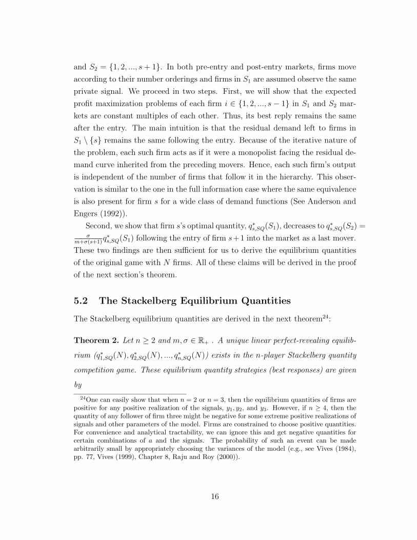
The Stackelberg equilibrium quantities are derived in the next theorem24:
Theorem 2. Let n ≥ 2 and m,σ ∈ R+ . A unique linear perfect-revealing equilib-
rium (q∗1,SQ(N), q∗2,SQ(N), ..., q∗n,SQ(N)) exists in the n-player Stackelberg quantity
competition game. These equilibrium quantity strategies (best responses) are given
by
24One can easily show that when n = 2 or n = 3, then the equilibrium quantities of firms arepositive for any positive realization of the signals, y1, y2, and y3. However, if n ≥ 4, then thequantity of any follower of firm three might be negative for some extreme positive realizations ofsignals and other parameters of the model. Firms are constrained to choose positive quantities.For convenience and analytical tractability, we can ignore this and get negative quantities forcertain combinations of a and the signals. The probability of such an event can be madearbitrarily small by appropriately choosing the variances of the model (e.g., see Vives (1984),pp. 77, Vives (1999), Chapter 8, Raju and Roy (2000)).
16
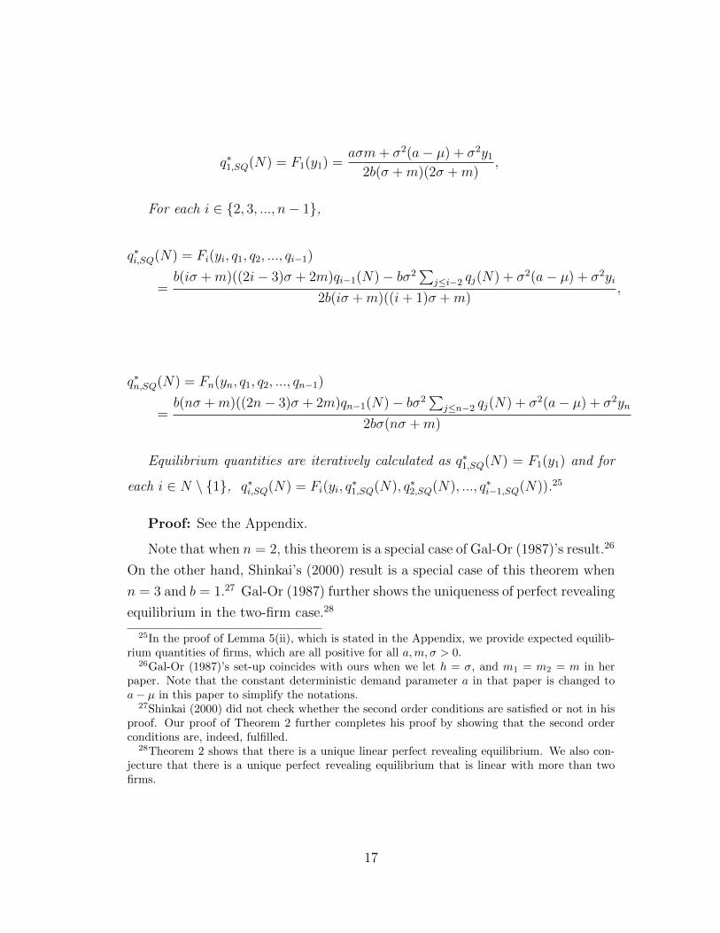
q∗1,SQ(N) = F1(y1) =aσm+ σ2(a− µ) + σ2y1
2b(σ +m)(2σ +m),
For each i ∈ {2, 3, ..., n− 1},
q∗i,SQ(N) = Fi(yi, q1, q2, ..., qi−1)
=b(iσ +m)((2i− 3)σ + 2m)qi−1(N)− bσ2
∑j≤i−2 qj(N) + σ2(a− µ) + σ2yi
2b(iσ +m)((i+ 1)σ +m),
q∗n,SQ(N) = Fn(yn, q1, q2, ..., qn−1)
=b(nσ +m)((2n− 3)σ + 2m)qn−1(N)− bσ2
∑j≤n−2 qj(N) + σ2(a− µ) + σ2yn
2bσ(nσ +m)
Equilibrium quantities are iteratively calculated as q∗1,SQ(N) = F1(y1) and for
each i ∈ N \ {1}, q∗i,SQ(N) = Fi(yi, q∗1,SQ(N), q∗2,SQ(N), ..., q∗i−1,SQ(N)).25
Proof: See the Appendix.
Note that when n = 2, this theorem is a special case of Gal-Or (1987)’s result.26
On the other hand, Shinkai’s (2000) result is a special case of this theorem when
n = 3 and b = 1.27 Gal-Or (1987) further shows the uniqueness of perfect revealing
equilibrium in the two-firm case.28
25In the proof of Lemma 5(ii), which is stated in the Appendix, we provide expected equilib-rium quantities of firms, which are all positive for all a,m, σ > 0.
26Gal-Or (1987)’s set-up coincides with ours when we let h = σ, and m1 = m2 = m in herpaper. Note that the constant deterministic demand parameter a in that paper is changed toa− µ in this paper to simplify the notations.
27Shinkai (2000) did not check whether the second order conditions are satisfied or not in hisproof. Our proof of Theorem 2 further completes his proof by showing that the second orderconditions are, indeed, fulfilled.
28Theorem 2 shows that there is a unique linear perfect revealing equilibrium. We also con-jecture that there is a unique perfect revealing equilibrium that is linear with more than twofirms.
17
5.3 Strategic Substitutes versus Strategic Complements
We say that quantity strategy qi is a strategic substitute (or complement respec-
tively) to quantity strategy qj, i 6= j, if the best response of firm i to an increase
in the quantity of firm j is to decrease (increase) its production (equivalently if∂2πi∂qi∂qj
< 0 (> 0) ). In this section, we investigate strategic substitutability versus
complementarity relationships among firms’ strategies in our Stackelberg setting.
One can use the best responses provided in Theorem 2 to find these relationships.
Lemma 2 summarizes our results.
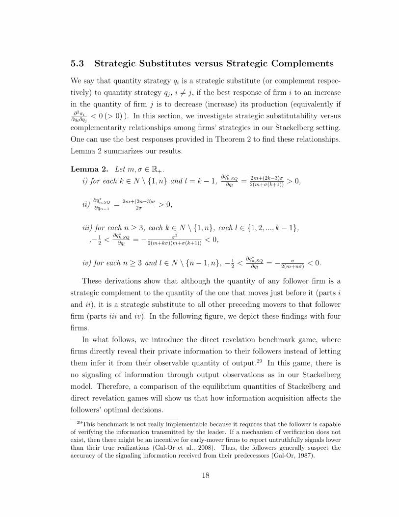
Lemma 2. Let m,σ ∈ R+.
i) for each k ∈ N \ {1, n} and l = k − 1,∂q∗k,SQ∂ql
= 2m+(2k−3)σ2(m+σ(k+1))
> 0,
ii)∂q∗n,SQ∂qn−1
= 2m+(2n−3)σ2σ
> 0,
iii) for each n ≥ 3, each k ∈ N \ {1, n}, each l ∈ {1, 2, ..., k − 1},,−1
2<
∂q∗k,SQ∂ql
= − σ2
2(m+kσ)(m+σ(k+1))< 0,
iv) for each n ≥ 3 and l ∈ N \ {n− 1, n}, −12<
∂q∗n,SQ∂ql
= − σ2(m+nσ)
< 0.
These derivations show that although the quantity of any follower firm is a
strategic complement to the quantity of the one that moves just before it (parts i
and ii), it is a strategic substitute to all other preceding movers to that follower
firm (parts iii and iv). In the following figure, we depict these findings with four
firms.
In what follows, we introduce the direct revelation benchmark game, where
firms directly reveal their private information to their followers instead of letting
them infer it from their observable quantity of output.29 In this game, there is
no signaling of information through output observations as in our Stackelberg
model. Therefore, a comparison of the equilibrium quantities of Stackelberg and
direct revelation games will show us that how information acquisition affects the
followers’ optimal decisions.
29This benchmark is not really implementable because it requires that the follower is capableof verifying the information transmitted by the leader. If a mechanism of verification does notexist, then there might be an incentive for early-mover firms to report untruthfully signals lowerthan their true realizations (Gal-Or et al., 2008). Thus, the followers generally suspect theaccuracy of the signaling information received from their predecessors (Gal-Or, 1987).
18
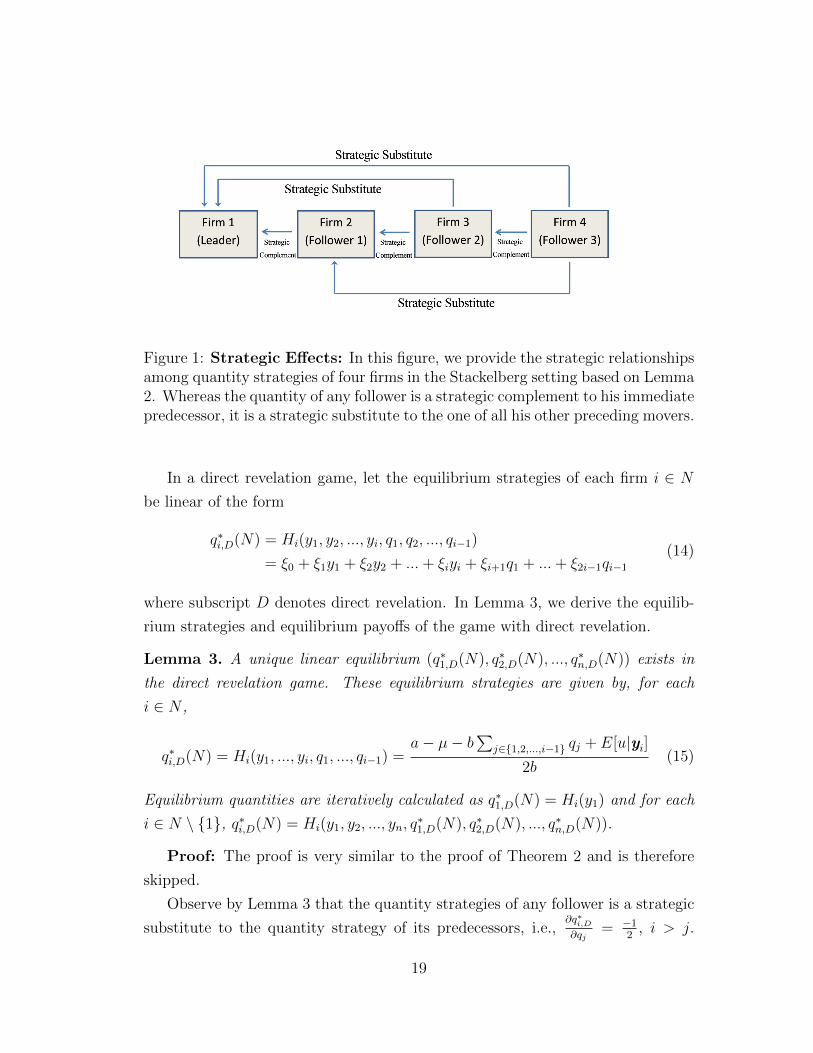
Figure 1: Strategic Effects: In this figure, we provide the strategic relationshipsamong quantity strategies of four firms in the Stackelberg setting based on Lemma2. Whereas the quantity of any follower is a strategic complement to his immediatepredecessor, it is a strategic substitute to the one of all his other preceding movers.
In a direct revelation game, let the equilibrium strategies of each firm i ∈ Nbe linear of the form
q∗i,D(N) = Hi(y1, y2, ..., yi, q1, q2, ..., qi−1)
= ξ0 + ξ1y1 + ξ2y2 + ...+ ξiyi + ξi+1q1 + ...+ ξ2i−1qi−1
(14)
where subscript D denotes direct revelation. In Lemma 3, we derive the equilib-
rium strategies and equilibrium payoffs of the game with direct revelation.
Lemma 3. A unique linear equilibrium (q∗1,D(N), q∗2,D(N), ..., q∗n,D(N)) exists in
the direct revelation game. These equilibrium strategies are given by, for each
i ∈ N ,
q∗i,D(N) = Hi(y1, ..., yi, q1, ..., qi−1) =a− µ− b
∑j∈{1,2,...,i−1} qj + E[u|yi]
2b(15)
Equilibrium quantities are iteratively calculated as q∗1,D(N) = Hi(y1) and for each
i ∈ N \ {1}, q∗i,D(N) = Hi(y1, y2, ..., yn, q∗1,D(N), q∗2,D(N), ..., q∗n,D(N)).
Proof: The proof is very similar to the proof of Theorem 2 and is therefore
skipped.
Observe by Lemma 3 that the quantity strategies of any follower is a strategic
substitute to the quantity strategy of its predecessors, i.e.,∂q∗i,D∂qj
= −12
, i > j.
19

Accordingly comparing this observation with the findings in Lemma 2 shows that
there exists a positive conjectural variation effect that is beneficial to the follower
firms in our Stackelberg model. This effect increases all slope parameters in the
best response functions of followers compared to a benchmark level of −1/2. From
the perspective of the last-mover, it does not really matter whether the information
is directly or indirectly revealed. However, indirect inferences about demand will
decrease non-last-movers’ preemptive abilities (i.e., first-mover advantages). It is,
therefore, this positive effect that might convert strategic substitutability relations
into strategic complementarity ones.
6 Stackelberg versus Cournot Oligopoly
6.1 Total Output and Price Comparisons
As prices are negatively correlated with total output, it is sufficient to show the
ranking of total equilibrium output between Cournot and Stackelberg compe-
titions. In that regard, define ∆E(Q∗(N)) as the difference of total expected
equilibrium production in the Cournot market from the one in the Stackelberg
market, i.e., ∆E(Q∗(N)) = E(Q∗C(N)) − E(Q∗SQ(N)). Our next theorem estab-
lishes that the simultaneous move game lead to higher total expected output and
lower expected price than the sequential move game irrespective of how noisy both
the demand shocks and firms’ private signals are.
Theorem 3. Let n ≥ 2 and m,σ ∈ R+. Whereas total expected equilibrium
market output is higher, the expected equilibrium price is lower in the Cournot
game than in the Stackelberg game. (i.e., ∆E(Q∗(N)) > 0)
Proof: See the Appendix.
We identify two effects that induce our result about output rankings between
Cournot and Stackelberg equilibrium outcomes. The first effect is the tradi-
tional first-mover advantage effect. Recall that the firms’ optimal decisions involve
strategic substitutability relationships in the absence of demand signaling through
outputs by Lemma 2. For this reason, each firm (save the last mover) selects a
20
high output in order to induce subsequent movers to cut back. Consequently,
the first-mover advantage induces total output to increase under the Stackelberg
competition (as compared to Cournot).
The second effect is the signaling effect30, which is absent under the Cournot
competition. As noted in the last section, followers become more responsive to the
output changes of their preceding movers under the positive conjectural variation
effect. That creates an incentive to invest in a lower capacity for the firms that
signal their demand information. Therefore, under the signaling effect, any non-
last mover firm would like to produce a low quantity to signal its followers that
the demand is low. In that regard, this negative output effect favors the Cournot
competition over the Stackelberg competition. In sum, there is one effect favoring
Stackelberg over Cournot and one effect favoring Cournot over Stackelberg. It
turns out that total negative output effects due to signaling information domi-
nate total positive output effects due to moving early. Thus, the total expected
equilibrium output is unambiguously higher in the Cournot case.
We finally consider the impact of these effects on the individual output levels
of firms when n = 2. Our results are summarized in Lemma 4.
Lemma 4. Let n = 2 and m,σ ∈ R+.
E[q∗2,SQ({1, 2})] > E[q∗C({1, 2})] > E[q∗1,SQ({1, 2})]
Proof: See the Appendix.
The leader firm faces both signaling and first-mover advantages effects unlike a
Cournot duopolist. Remark by Lemma 2 that the reaction function of the follower
is upwards sloping. Therefore, the leader firm’s output reduction incentive, which
is induced by the signaling effect, is likely to dominate its output expansion incen-
tive, which is induced by the first-mover advantages. Consequently, it produces
less than a Cournot duopolist in expectation. Nevertheless, since the follower firm
does not face any of above effects, it can increase its output aggressively through
strategic complementarity. Indeed, it produces more than a Cournot duopolist in
expected terms.
30In a set-up where two retailers infer demand information from the price chosen by onemanufacturer., Gal-Or et al. (2008, 2011) identify the presence of an inference effect, which isthe cousin of signaling effect in price setting games. Specifically, because of this inference effect,the manufacturer would like to set a low wholesale price to signal to the retailer that the demandis low.
21
6.2 Profit, Consumer- and Total Surplus Comparisons
In this section, we provide our main results. We compare total expected equi-
librium profit, consumer surplus and total surplus between the Stackelberg and
Cournot competitions. We start with the total expected profit comparisons. Total
expected equilibrium profit is defined as
E[Π∗(N)] = E[p∗Q∗(N)] = E[(a− µ+ u− bQ∗(N))Q∗(N)] (16)
Now, let the total expected profit difference between these models be denoted as
∆E(Π∗(N)) = E(Π∗C(N))− E(Π∗SQ(N)) = nE(π∗C(N))−∑
i∈N E(π∗i,SQ(N)).
Theorem 4. Let n ∈ {2, 3, 4, 5} and m,σ ∈ R+. Total expected profit is higher
in the Stackelberg game than in the Cournot game.31 (i.e., ∆E(Π∗(N)) < 0)
Proof: See the Appendix.
Before providing the main effects that generate the total profit rankings in
this theorem, we derive consumer surplus and total welfare rankings between our
models. Ex-ante total expected equilibrium welfare can be deduced by summing
up consumer and producer surplus, which are respectively defined in (1) and (16),
as:
E[TW ∗(N)] = E[(a− µ+ u)Q∗(N)− b(Q∗(N))2
2] (17)
Based on this definition, let ∆E(TW ∗(N)) be the difference of the Cournot
competition total equilibrium welfare from the Stackelberg competition total equi-
librium welfare, i.e., ∆E(TW ∗(N)) = E(TW ∗C(N)) − E(TW ∗
SQ(N)). Similarly,
the same difference for the consumer surpluses is defined as ∆E(CS∗(N)) =
E(CS∗C(N))− E(CS∗SQ(N)). Next, we present a main result.
31Proving this claim in a general n−firm framework requires tedious algebraic calculations.Given this constraint, we prove the claims up to a 5−firm set-up and conjecture that the claimshold with more than five firms.
22
Theorem 5. Let n ∈ {2, 3, 4, 5} and m,σ ∈ R+. Both consumer and total ex-
pected equilibrium welfare are higher under the Cournot competition than under
the Stackelberg competition.32 (i.e., ∆E(TW ∗(N)) > 0 and ∆E(CS∗(N)) > 0.)
Proof: See the Appendix.
As previously discussed, first-mover advantages increase early-mover firms’
production incentives to capture a bigger pie of the market. This increase in out-
put levels translates into not only higher consumer surplus and total welfare but
also lower total profits as noted under perfect information models that compare
Stackelberg and Cournot competitions. By analogy, the adverse consequences of
the signaling effect on output investment incentives of the early-mover firms is
expected to generate lower consumer surplus and total welfare; and higher total
profits. As a result, the domination of the signaling effect over the first-mover
advantages effect partially explains the observed rankings between two types of
competition in Theorem 5.
Apart from the above two opposite output effects, we finally point out two wel-
fare effects in order to completely justify the rankings in Theorem 5. These two
effects are called as the information acquisition effect and negative externalities of
information acquisition effect. They do not account for total output differences,
but rather they give the possibility that even when the expected outputs are the
same between two types of competition, total profit, consumer surplus, and total
welfare rankings are likely to be different. Specifically, the followers are better
informed than their predecessors in a leader-followers game. Therefore, they are
likely to produce more when the demand is high and produce less when it is low
under the Stackelberg competition compared to the Cournot competition. This
implies that prices are less responsive to the underlying demand shock under the
Stackelberg competition. This greater price stability (and higher output produc-
tion volatility) induces higher welfare, implying that the information acquisition
effect favors Stackelberg over Cournot in terms of total profits, consumer surplus
and total welfare.33
32See Footnote 31.33The intuition is similar to the welfare effects of third degree price discrimination, where third
degree price discrimination (lower price stability) reduces welfare when the expected quantitiesare the same.
23
Information acquisition of a follower firm also imposes a negative externality to
its competitor(s) in the following sense. Since demand shocks are common for all
firms, a more informed follower firm lead the residual demand of its competitor(s)
less variable. This lower variability in the demand intercept of the competitor
firms would translate into lower total welfare if they have some prior of demand
initially as in our set-up. Therefore, this effect is likely to decrease total welfare.
That implies that negative externalities of information acquisition effect favors
the Cournot competition over the Stackelberg competition in welfare terms.
Among these four effects, the signaling and negative externalizes of information
acquisition effects are the dominant ones. Accordingly, the Cournot mode of
conduct is socially desirable compared to the Stackelberg mode of conduct from
both consumer and total welfare point of views. This result sharply diverges from
traditional efficiency rankings between these two game settings.
We now study two simple examples in order to better understand these two
welfare effects. In the first one, we let each firm a monopoly for the good it pro-
duces in a duopoly set-up. Since demand intercepts are common for both firms,
the follower firm still learns the signal of the leader firm in a perfect revealing
equilibrium. Hence this type of information acquisition affects the welfare anal-
ysis between Cournot and Stackelberg competitions. In the second example, we
provide more intuition about the welfare effects of the negative externalities of
information acquisition of firms on their competitors.
Example 1: Let N = {1, 2} and pi = a− µ+ u− bqi, i = 1, 2, where b > 0 is
the slope of demand. We follow all other assumptions of our original model. The
Stackelberg perfect revealing equilibrium outputs of firms will be derived in the
extension Section 7.5 as
q∗1,DS =a
2b+σ(y1 − µ)
2b(m+ σ)and q∗2,DS =
a
2b+σ(y1 + y2 − 2µ)
2b(m+ 2σ)(18)
where DS refers to the differentiated Stackelberg game. Similarly, Cournot-
Bayesian equilibrium outputs of firms are given as
q∗i,DC =a
2b+
σ(yi − µ)
2b(m+ σ)i = 1, 2 (19)
where DC corresponds to the differentiated Cournot game. Note that from the
24
perspective of the first firm, it does not make any difference whether the type of
competition is Cournot or Stackelberg. It simply produces the monopoly level of
output in both set-ups. Therefore, q∗1,DS = q∗1,DC . However, since the signal of the
leader is revealed to the follower under the Stackelberg competition, the follower
is more informed about demand as the compared to the Cournot competition.34
Comparing (18) and (19) shows that the follower is able to produce more when
the observed signal of the leader is greater than mµ+σy2m+σ
as compared to a Cournot
duopolist. For example, consider y2 = µ. Firm two produces a/2b under the
Cournot competition. However, the Stackelberg follower produces more than a/2b,
when the observed signal of the leader is greater than the average (i.e., y1 > µ).
That implies that there is additional consumer surplus, producer surplus and total
surplus generated by producing more in the high states of demand. The opposite
is true when the leader’s realization of the state of demand is lower than mµ+σy2m+σ
.
Nevertheless, the gain in higher states of demand in welfare grounds overwhelms
the loss in lower states of demand with a linear demand curve.35 Therefore,
although the expected output of a firm under both mode of conducts are the
same, expected- total profits, consumer surplus, and total welfare are all higher
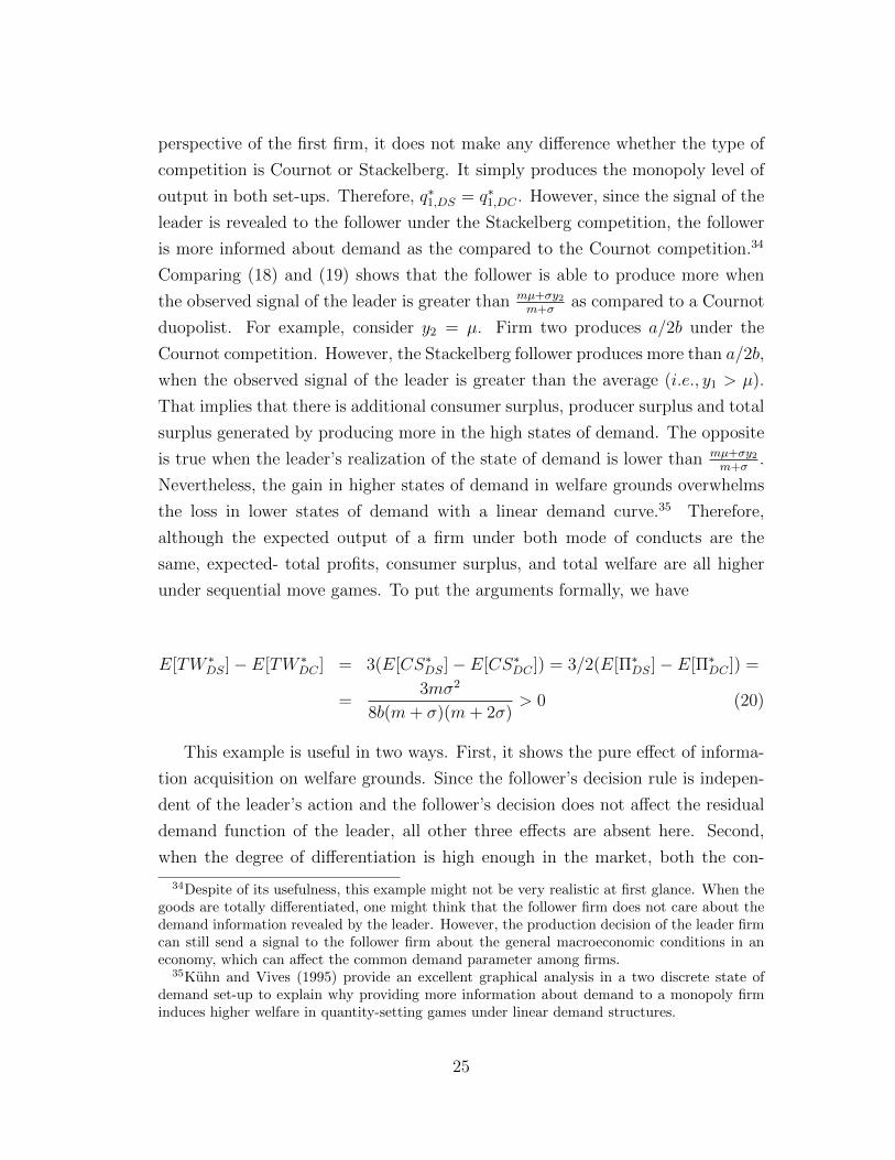
under sequential move games. To put the arguments formally, we have
E[TW ∗DS]− E[TW ∗
DC ] = 3(E[CS∗DS]− E[CS∗DC ]) = 3/2(E[Π∗DS]− E[Π∗DC ]) =
=3mσ2
8b(m+ σ)(m+ 2σ)> 0 (20)
This example is useful in two ways. First, it shows the pure effect of informa-
tion acquisition on welfare grounds. Since the follower’s decision rule is indepen-
dent of the leader’s action and the follower’s decision does not affect the residual
demand function of the leader, all other three effects are absent here. Second,
when the degree of differentiation is high enough in the market, both the con-
34Despite of its usefulness, this example might not be very realistic at first glance. When thegoods are totally differentiated, one might think that the follower firm does not care about thedemand information revealed by the leader. However, the production decision of the leader firmcan still send a signal to the follower firm about the general macroeconomic conditions in aneconomy, which can affect the common demand parameter among firms.
35Kuhn and Vives (1995) provide an excellent graphical analysis in a two discrete state ofdemand set-up to explain why providing more information about demand to a monopoly firminduces higher welfare in quantity-setting games under linear demand structures.
25
sumer surplus and total welfare are no longer higher in simultaneous move-games
by continuity of the parameter values. In other words, some of our main results
of the paper will not be robust when firms produce almost monopoly products.
Nevertheless, we will see in Section 7.5 that our main results hold for a very wide
range of parameter values in a differentiated good environment.
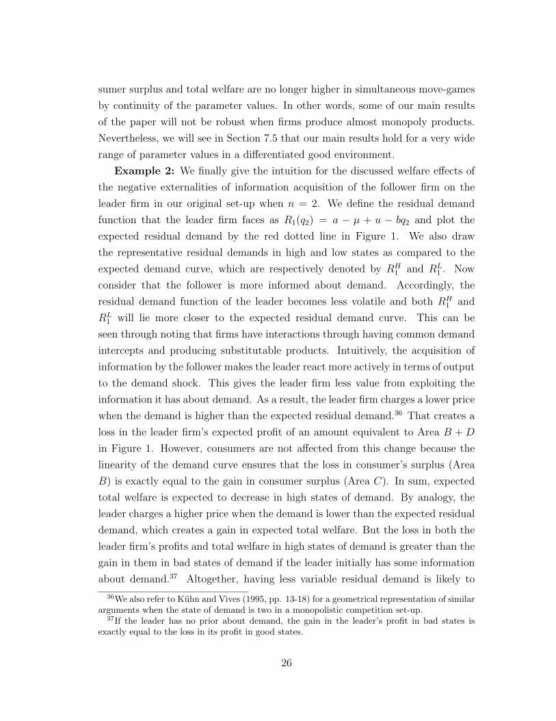
Example 2: We finally give the intuition for the discussed welfare effects of
the negative externalities of information acquisition of the follower firm on the
leader firm in our original set-up when n = 2. We define the residual demand
function that the leader firm faces as R1(q2) = a − µ + u − bq2 and plot the
expected residual demand by the red dotted line in Figure 1. We also draw
the representative residual demands in high and low states as compared to the
expected demand curve, which are respectively denoted by RH1 and RL
1 . Now
consider that the follower is more informed about demand. Accordingly, the
residual demand function of the leader becomes less volatile and both RH1 and
RL1 will lie more closer to the expected residual demand curve. This can be
seen through noting that firms have interactions through having common demand
intercepts and producing substitutable products. Intuitively, the acquisition of
information by the follower makes the leader react more actively in terms of output
to the demand shock. This gives the leader firm less value from exploiting the
information it has about demand. As a result, the leader firm charges a lower price
when the demand is higher than the expected residual demand.36 That creates a
loss in the leader firm’s expected profit of an amount equivalent to Area B + D
in Figure 1. However, consumers are not affected from this change because the
linearity of the demand curve ensures that the loss in consumer’s surplus (Area
B) is exactly equal to the gain in consumer surplus (Area C). In sum, expected
total welfare is expected to decrease in high states of demand. By analogy, the
leader charges a higher price when the demand is lower than the expected residual
demand, which creates a gain in expected total welfare. But the loss in both the
leader firm’s profits and total welfare in high states of demand is greater than the
gain in them in bad states of demand if the leader initially has some information
about demand.37 Altogether, having less variable residual demand is likely to
36We also refer to Kuhn and Vives (1995, pp. 13-18) for a geometrical representation of similararguments when the state of demand is two in a monopolistic competition set-up.
37If the leader has no prior about demand, the gain in the leader’s profit in bad states isexactly equal to the loss in its profit in good states.
26
decrease not only the leader’s profits but also total welfare while leaving consumer
surplus unchanged.
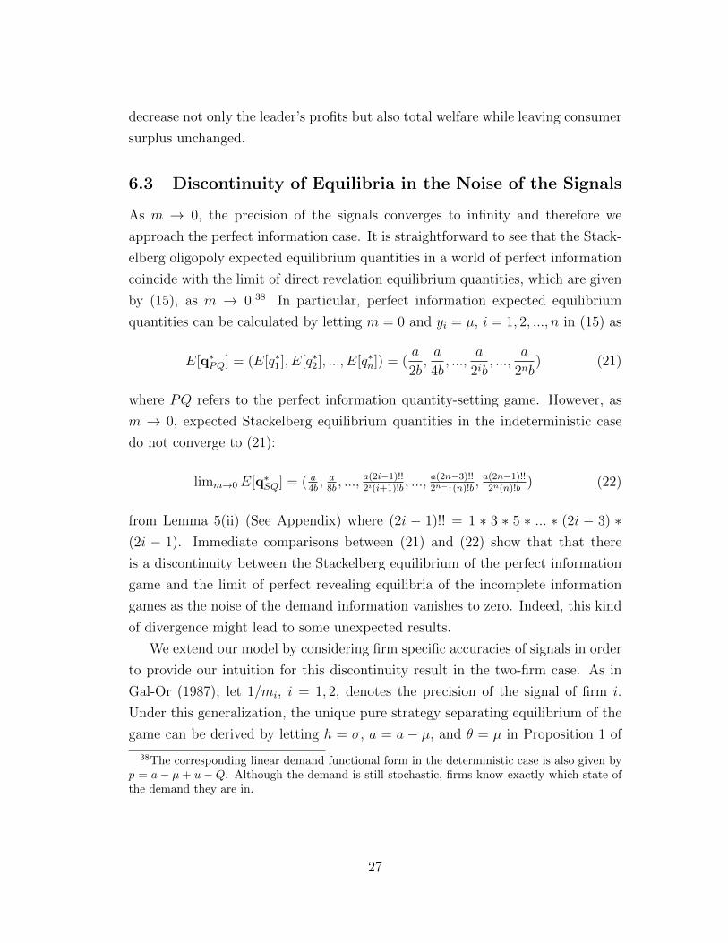
6.3 Discontinuity of Equilibria in the Noise of the Signals
As m → 0, the precision of the signals converges to infinity and therefore we
approach the perfect information case. It is straightforward to see that the Stack-
elberg oligopoly expected equilibrium quantities in a world of perfect information
coincide with the limit of direct revelation equilibrium quantities, which are given
by (15), as m → 0.38 In particular, perfect information expected equilibrium
quantities can be calculated by letting m = 0 and yi = µ, i = 1, 2, ..., n in (15) as
E[q∗PQ] = (E[q∗1], E[q∗2], ..., E[q∗n]) = (a
2b,a
4b, ...,
a
2ib, ...,
a
2nb) (21)
where PQ refers to the perfect information quantity-setting game. However, as
m → 0, expected Stackelberg equilibrium quantities in the indeterministic case
do not converge to (21):
limm→0E[q∗SQ] = ( a4b, a
8b, ..., a(2i−1)!!
2i(i+1)!b, ..., a(2n−3)!!
2n−1(n)!b, a(2n−1)!!
2n(n)!b) (22)
from Lemma 5(ii) (See Appendix) where (2i − 1)!! = 1 ∗ 3 ∗ 5 ∗ ... ∗ (2i − 3) ∗(2i − 1). Immediate comparisons between (21) and (22) show that that there
is a discontinuity between the Stackelberg equilibrium of the perfect information
game and the limit of perfect revealing equilibria of the incomplete information
games as the noise of the demand information vanishes to zero. Indeed, this kind
of divergence might lead to some unexpected results.
We extend our model by considering firm specific accuracies of signals in order
to provide our intuition for this discontinuity result in the two-firm case. As in
Gal-Or (1987), let 1/mi, i = 1, 2, denotes the precision of the signal of firm i.
Under this generalization, the unique pure strategy separating equilibrium of the
game can be derived by letting h = σ, a = a − µ, and θ = µ in Proposition 1 of
38The corresponding linear demand functional form in the deterministic case is also given byp = a − µ + u −Q. Although the demand is still stochastic, firms know exactly which state ofthe demand they are in.
27
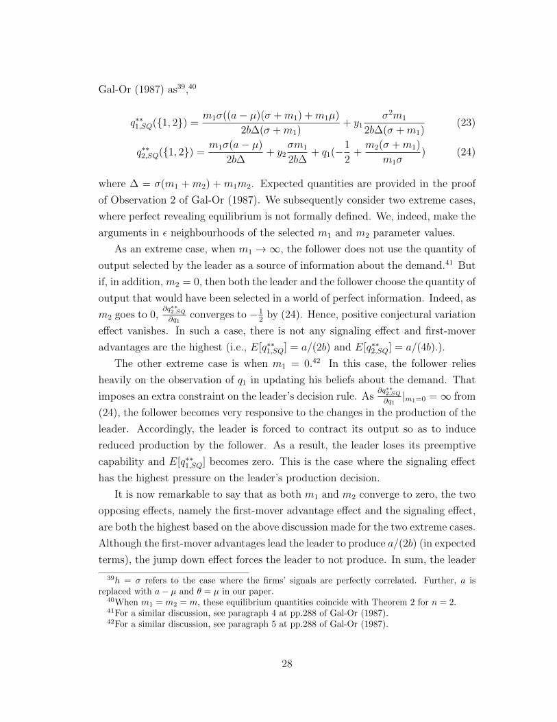
Gal-Or (1987) as39,40
q∗∗1,SQ({1, 2}) =m1σ((a− µ)(σ +m1) +m1µ)
2b∆(σ +m1)+ y1
σ2m1
2b∆(σ +m1)(23)
q∗∗2,SQ({1, 2}) =m1σ(a− µ)
2b∆+ y2
σm1
2b∆+ q1(−1
2+m2(σ +m1)
m1σ) (24)
where ∆ = σ(m1 + m2) + m1m2. Expected quantities are provided in the proof
of Observation 2 of Gal-Or (1987). We subsequently consider two extreme cases,
where perfect revealing equilibrium is not formally defined. We, indeed, make the
arguments in ε neighbourhoods of the selected m1 and m2 parameter values.
As an extreme case, when m1 →∞, the follower does not use the quantity of
output selected by the leader as a source of information about the demand.41 But
if, in addition, m2 = 0, then both the leader and the follower choose the quantity of
output that would have been selected in a world of perfect information. Indeed, as
m2 goes to 0,∂q∗∗2,SQ∂q1
converges to −12
by (24). Hence, positive conjectural variation
effect vanishes. In such a case, there is not any signaling effect and first-mover
advantages are the highest (i.e., E[q∗∗1,SQ] = a/(2b) and E[q∗∗2,SQ] = a/(4b).).
The other extreme case is when m1 = 0.42 In this case, the follower relies
heavily on the observation of q1 in updating his beliefs about the demand. That
imposes an extra constraint on the leader’s decision rule. As∂q∗∗2,SQ∂q1|m1=0 =∞ from
(24), the follower becomes very responsive to the changes in the production of the
leader. Accordingly, the leader is forced to contract its output so as to induce
reduced production by the follower. As a result, the leader loses its preemptive
capability and E[q∗∗1,SQ] becomes zero. This is the case where the signaling effect
has the highest pressure on the leader’s production decision.
It is now remarkable to say that as both m1 and m2 converge to zero, the two
opposing effects, namely the first-mover advantage effect and the signaling effect,
are both the highest based on the above discussion made for the two extreme cases.
Although the first-mover advantages lead the leader to produce a/(2b) (in expected
terms), the jump down effect forces the leader to not produce. In sum, the leader
39h = σ refers to the case where the firms’ signals are perfectly correlated. Further, a isreplaced with a− µ and θ = µ in our paper.
40When m1 = m2 = m, these equilibrium quantities coincide with Theorem 2 for n = 2.41For a similar discussion, see paragraph 4 at pp.288 of Gal-Or (1987).42For a similar discussion, see paragraph 5 at pp.288 of Gal-Or (1987).
28
ends up producing at an intermediate level, which is a/(4b). That induces the
follower to produce 3a/(8b) in expected terms rather than the perfect information
outcome a/(4b). Hence we get the observed discontinuity as m approaches to zero
and the signaling distortions play an important role in this nontrivial result. We
conjecture that a similar argument to above can be made in an n−firm case and
therefore we skip it.
Based on the above discussion, the study herein does not have a conclusion
that perfect information outcomes are never achievable as a limit of Stackelberg
perfect revealing equilibria. For example, if the precision of the leader’s signal is
very uninformative as compared to the follower and the firms’ private signals are
perfectly correlated, then the Stackelberg duopoly perfect revealing equilibrium
strategies might still be close to the Stackelberg perfect information outcomes
as noted above. However, Gal-Or argues that, if the firms’ private signals are
sufficiently uncorrelated, then we still have significant divergences from perfect
information outcomes for a wide range of parameter values even with asymmetric
precision of signals. For instance, she shows that if the degree of correlation of
signals (denoted by h) changes between 0 and 2σ/3, then the reaction function
of the follower is upwards sloping at any m1,m2 ∈ R+. Having said that, our
reversal rankings between the Cournot and Stackelberg equilibrium outcomes are
also expected to hold for this very large set of parameter values.43
7 Discussions and Extensions
7.1 Firm Asymmetries and Concentration
Concentration is mostly thought to be a cause for concern.44 This concern is
based on an intuition derived mainly from considering the symmetric equilibrium
43For instance, we first introduce the Cournot competition in Gal-Or’s two-firm set-up withdemand uncertainty. After some involved calculations, one can show that total expected (unique)Cournot equilibrium quantity is 2a/3b as in our baseline Cournot model. Subtracting totalexpected Stackelberg equilibrium outputs (provided in the proof of Observation 2 of Gal-Or’s
paper) from total expected Cournot equilibrium quantity yields a(h2+(m1+σ)(2σ−3h+2m2))12b∆ , which
is positive at any h ∈ (0, 2σ/3] and m1,m2 ∈ R+. Accordingly, the equilibrium price is higherunder the Stackelberg competition than under the Cournot competition for this set of parametervalues.
44This paragraph is mostly adopted from Daughety (1990).
29
of oligopoly models. As the number of firms in the symmetric equilibrium in-
creases, some measures of welfare rises (e.g., total surplus) and some measures
of concentration falls (e.g., The Herfindahl-Hirschman Index (or HHI)). However,
the differences in firm sizes can also be a cause of concentration. Daughety argues
that the foregoing intuition does not carry over to the asymmetric equilibria which
seemingly reflect a more realistic picture of the world. His findings in a world of
perfect information about demand suggest that social optimality may involve ex-
tensive asymmetries in firm sizes. These contradicting results indicate that the
sign of the correlation between concentration indexes and welfare is ambiguous.
In the light of these concerns, we analyze how firm asymmetries affect social
optimality in our set-up. The HHI is a measure of the size of firms in relation to the
industry and is widely accepted by the anti-trust agencies to be an indicator of the
amount of concentration among firms. It is defined as H =∑n
i=1(E[si])2, where
E[si] = E[qi]/E[Q(N)] is the expected market share of firm i with∑n
i=1E[si] = 1.
Remark that as the timing of producing is different under the Stackelberg model,
firms have asymmetric market shares. Therefore, the Stackelberg model yields
a higher HHI than does the Cournot model, where firms behave symmetrically.
In other words, the market is more concentrated under the Stackelberg mode of
conduct than under the Cournot mode of conduct. In what follows, we relate our
main findings with concentration.
7.2 Welfare and Concentration
Daughety (1990) argues that concentration measures (such as HHI) provide little
insight about welfare. His findings reflect that increases in such measures some-
times reflect increases in welfare and sometimes reflect decreases in welfare. For
example, as we switch from Cournot to Stackelberg model, both the HHI index
and total welfare increase.45 In that regard, asymmetry, thus concentration, is
beneficial from society’s viewpoint. This observation contradicts to the standard
IO paradigm that a higher market concentration leads to less competition in the
market and therefore is harmful for the society. Nevertheless, this result does
45It has already been stated in the related literature section that Daughety studies a two-stagemodel, where m leaders and n −m followers compete. Apart from the incomplete informationabout demand extension, our model coincides with his model at m = 0 or m = 2 (Cournot) andm = 1 (Stackelberg) when n = 2. In the future, we are planning to study Daughety’s model inour incomplete information setting to better assess the link between concentration and welfare.
30

not take into account the possibility that early moving firms’ quantity strategies
might send demand signals to the late-movers in a stochastic demand environ-
ment. In such a set-up, total welfare ranking between Stackelberg and Cournot
competitions are reversed in an n−firm oligopoly model (n ≤ 5) irrespective of
how noisy both the demand shocks and private demand signals of firms are by
Theorem 5. This result suggests that the traditional IO paradigm is likely to be
preserved when firm’s strategies involve learning about demand from the actions
of their competitors. Therefore, HHI provides significant amount of insight about
welfare. A policy maker would then prefer the less concentrated Cournot indus-
tries over the more concentrated Stackelberg industries if he/she has an impact
on the determination of market’s mode of conduct.
7.3 Profits, Prices and Concentration
A similar implication holds for the relationships of prices and profits with con-
centration. In study after study, a positive correlation of prices and average firm
profits with various measures of concentration has been found as we have already
noted in the introduction.46 Unfortunately, perfect information about demand
models may fail to support these empirical results. Specifically, a higher concen-
tration, which is caused by switching from the Coutnot model to the Stackelberg
model, is likely to be associated with both lower average firm profits and lower
prices. But remark by Theorems (3) and (4) that the more concentrated Stackel-
berg competition generates both higher total profits and higher prices than does
the less concentrated Cournot competition. Therefore, our foregoing analysis in a
world of incomplete information can partially support these empirical results.
7.4 Merger Incentives and Concentration
As a last application, we perform a merger analysis to answer an important policy
question: Are mergers easier to be allowed under more concentrated or less con-
centrated industries? We consider a cost-efficient horizontal merger to monopoly
46Price-concentration studies are widely thought to overcome potential problems on profit-concentration ratios. For example, prices are much more easily observed than economics profits.Further, they are not subject to the many accounting conventions that complicate studyingprofits.
31
in both Cournot and Stackelberg duopoly markets.47 Our previous set-up and
assumptions about the parameters of the model is still valid. However, we con-
sider firms that have symmetric marginal costs, i.e., c, in the pre-merger case.
Accordingly, the deterministic demand parameter a can be considered as net of
the marginal cost level of firms, i.e., a = a − c. Following a merger, we assume
that there are efficiency gains and the merged firm’s marginal cost level becomes
ce, where ce ∈ [0, c). Accordingly, let a = a − c + ce. Our welfare analysis and
comparisons between simultaneous and sequential move settings performed in the
main text corresponds to the pre-merger case. We now let two firms merge to a
monopoly horizontally. Under both Cournot and Stackelberg competitions, the
merged firm maximizes the expected joint profits of firms one and two.
maxq1,q2
E[πM ] = E[(a− µ+ u− b(q1 + q2))(q1 + q2)|y1, y2] (25)
where πM denotes the total profits of the merged firm. Since the merged firm’s
problem is symmetric between its facilities, then FOC’s yield equilibrium quanti-
ties as
q∗1 = q∗2 =a− µ+ E[u|y1, y2]
4b(26)
Based on (4) and (26), the post-merger expected welfare under both types of
competitions reduces to
TW ∗M =
3a2(m+ 2σ) + 6σ2
8b(m+ 2σ)(27)
We assume that a merger is allowed if it generates sufficiently large efficiency gains
to increase total welfare.
Theorem 6. Let n = 2. The minimum level of efficiency gains to allow mergers
to monopoly is lower under the Stackelberg competition than under the Cournot
competition.
Proof: See the Appendix.
47Since our main concern of the paper is not to explain the relationship between mergerincentives of firms and market concentration, we just wanted to give the main intuition bystudying a simple horizontal merger model. One can come up with a more sophisticated mergermodel that does not necessarily lead mergers to monopoly.
32
Based on this lemma, anti-trust authorities can be more suspicious about
mergers in symmetric industries. The main intuition is easy to see. Since the
post-merger welfare is the same under both Cournot and Stackelberg competi-
tions, then the pre-merger welfare is the determinant factor in answering our
policy question. But since the pre-merger welfare is lower under the Stackelberg
competition than under the Cournot competition (but not under perfect informa-
tion about demand), then it would be reasonable to require less efficiency gains
to allow mergers in more concentrated Stackelberg industries. In addition, the
highest level of post-merger concentration is achieved under both types of mar-
kets as both firms merge to monopoly. Hence, market concentration is likely to
be increased more after a merger in less concentrated pre-merger industries (i.e.,
Cournot). That also partially explains why FTC directs its resources toward
horizontal mergers that are made among firms that most increased market con-
centration as it requires less efficiency gains to allow mergers. Altogether, mergers
are more likely in more concentrated industries.
7.5 Differentiated Products
We have assumed that firms produce homogeneous products until this section.
We would like to discuss the robustness of our results in an environment where
two firms produce heterogeneous products. Let there be two firms competing in
quantities. Each firm i (=1,2) produces a differentiated product at a price level
of pi and at a production level of qi. The representative consumer maximizes
consumer surplus
maxqi
CS = (a− µ+ u)(q1 + q2)− b(q21+q22)
2− bλq1q2 −
∑2j=1 pjqj (28)
where a > µ > 0, u is a random variable with mean µ and variance σ, a is the
observed market demand parameter by all firms, b is the slope of the demand, and
λ ∈ [0, 1] is an inverse measure of product differentiation in the market. When
λ = 1, products are perfect substitutes and no longer differentiable as in the main
text. On the other hand, when λ = 0, products are unrelated and each firm is a
monopoly for the product it produces. The maximization problem in (28) yields
33
a linear demand curve with a stochastic term in the intercept:
pi = a− µ+ u− bqi − bλqj, i 6= j, i, j = 1, 2 (29)
We normalize the unit cost of production to zero.
No firm can observe the realized value of the prior random variable u, but each
firm i can observe the realized value of its own private signal yi on u. Let both u
and each yi (i = 1, 2, ..., n) have a full positive support. we refer to Section 3 for
further assumptions on the prior u and private signals y1 and y2.48
We now present both Cournot and Stackelberg duopoly models with heteroge-
nous products. Later, we compare both models.
7.5.1 Differentiated Cournot Duopoly Model
We first assume that two firms simultaneously decide their quantities after getting
their private signals about demand. Since firms cannot draw inferences about the
private signals of their competitors, each firm’s equilibrium quantity strategy only
depends on its own signal.
Theorem 7. Let n = 2 and m,σ ∈ R+ . The unique Bayesian equilibrium of the
differentiated Cournot game is (q∗1,DC , q∗2,DC), where
q∗i,DC =a
b(2 + λ)+
σ(yi − µ)
b(2m+ σ(2 + λ)), i = 1, 2 (30)
Proof: See the Appendix.
When λ = 1, the competition among firms is fierce as goods are perfect sub-
stitutes of each other as we assumed in the baseline model. Note also that the
Cournot equilibrium quantities in Theorem 1 at n = 2 and b = 1 coincide with
the ones in Theorem 7 at λ = 1. On the other extreme, when firms are monop-
olies for the good they produce (λ = 0), the expected monopoly quantity is a/2
which is the same with the one in the perfect information case. This observation
is consistent with our findings under quantity competition stated in Section 4.
48We apologize for this economic way of presenting this model.
34
7.5.2 Differentiated Stackelberg Duopoly Model
In the Stackelberg model, we assume that each firm chooses its quantity level after
observing the private signal but before realizing the actual demand. Without loss
of any generality, suppose firm one, being the Stackelberg leader, first chooses
its quantity level, then does firm two (follower) after observing the quantity level
chosen by the leader. Let R+ and Yi denote the pure strategy space and firm i’s
private signal’s strategy space respectively. Firm one chooses its optimal quantity
level after observing its private signal y1. Its strategy is denoted by G1(y1) where
G1 : Y1 → R+. Firm two can condition its optimal quantity level on both its
private signal y2 and on the quantity level q1 chosen by the leader. Hence, its
optimal strategy is denoted by G2(y2, p1) where G2 : Y2 ×R+ → R+.
As before, we focus on perfect revealing equilibria, which can be defined in a
similar fashion to the one in the main text. Formally,
DEFINITION. A strategy combination (q∗1,DS, q∗2,DS) is a Stackelberg perfect
revealing equilibrium if it satisfies the following two-system of equations:
∀y1 ∈ Y1,
q∗1,DS = G1(y1) = argmaxq1∈R+
E[π1(q1, G2(y2, q1), u)|y1]
∀y2 ∈ Y2,∀G1(y1) = q1 ∈ R+,
q∗2,DS = G2(y2, q1) = argmaxq2∈R+
E[π2(q1, q2, u)|y2, q1]
(31)
where DS refers to the differentiated Stackelberg quantity competition.
In order to derive the Stackelberg perfect revealing equilibrium, we conjecture
that firms have linear equilibrium quantity strategies. Accordingly, let q∗1,DS =
α0 + α1y1 and q∗2,DS = β0 + β1y2 + β3q1 for some constants α0, α1, β0, β1, β1 ∈ R+.
In the proof of Theorem 8, we derive these constants and obtain the equilibrium
quantities.
Theorem 8. Let n = 2, m,σ ∈ R+, and λ ∈ [0, 1]. Under Assumption 1, a unique
linear perfect revealing equilibrium (q∗1,DS, q∗2,DS) exists in the two-player differen-
tiated Stackelberg (DS) quantity competition game. These equilibrium quantity
35
strategies (best responses) are given by
q∗1,DS = G1(y1) = (2m(1−λ)+σ(4−3λ))(am+(a−µ+y1)σ)2b(m+σ)(m+2σ)(2−λ2)
,
q∗2,DS = G2(y2, q1) = (a−µ+y2)σ2b(m+2σ)
+ q1( (2−λ(2−λ))m+2(1−λ)2σ2(1−λ)m+(4−3λ)σ
− λ2)
Equilibrium quantities are iteratively calculated as q∗1,DS = G1(y1) and q∗2,DS =
G2(y2, q∗1,DS).
Proof: See the Appendix.
As a > µ by assumption, both q∗1,DS and q∗2,DS are positive for any posi-
tive realizations, i.e., y1 and y2. Observe also by Theorem 8 that∂q∗2,DS∂q1
=(2−λ)(2m+(2−λ)σ)4(1−λ)m+2(4−3λ)σ
> 0. Therefore, the equilibrium quantity of the follower is a
strategic complement to the leader’s quantity for any degree of heterogeneity
among products.
We are now ready to compare differentiated Cournot and Stackelberg quantity
competitions in terms of expected- quantities, total profits, consumer surplus, and
total welfare.
7.5.3 Differentiated Cournot versus Differentiated Stackelberg
Define expected equilibrium total profits as E[ΠD] = E[p1q1 + p2q2] where the
subscript D refers to product differentiation. Adding profits to consumer surplus
given in (28) and taking an expectation over the resulting equation yields expected
total welfare as
E[TWD] = E[(a− µ+ u)(q1 + q2)− b(q21 + q2
2)
2− bλq1q2] (32)
Now denote the difference between differentiated- Cournot and Stackelberg
equilibrium outcomes as ∆E[l∗D] = E[l∗DC ]− E[l∗DS] for l ∈ {Q,Π, CS, TW}. The
next theorem compares expected- total outputs and total profits of firms between
differentiated Stackelberg and Cournot competitions.
Theorem 9. Let n = 2 and m,σ ∈ R+.
36
i) For λ ∈ (0, 1], ∆E[Q∗D] > 0 and for λ = 0, ∆E[Q∗D] = 0.
ii) For λ ∈ [0, 1] and a ≥ σ, we have ∆E[Π∗D] < 0.49
Proof: See the Appendix.
Based on Theorem 9, both expected total outputs and total profits are higher
under the Cournot competition than under the Stackelberg competition for any
degree of substitution between products. This result suggests that output and
total profit rankings stated respectively in Theorems 3 and 4 are robust to the
product differentiation.
Theorem 10. Let n = 2 and m,σ ∈ R+.
i)∂∆E[CS∗D]
∂a> 0 and
∂∆E[TW ∗D]
∂a> 0.
ii) For a ≥ 3σ and λ ∈ [0.1, 1], we have ∆E[CS∗D] > 0 and ∆E[TW ∗D] > 0.50
Proof: See the Appendix.
We have already concluded in Example 1 of Section 6.2 that when λ = 0, both
rankings stated in Theorem 10(ii) are reversed. However, this theorem shows that
for sufficiently high and reasonable deterministic demand parameter a, homoge-
neous good model rankings of equilibrium welfare and consumer surplus between
Cournot and Stackelberg models are preserved for a degree of substitution level
greater than 0.1 between firms’ products. Hence, even when firms produce differ-
entiated products, the effects of signaling and negative externalities of information
acquisition outweighes the effects of information acquisition and first-mover ad-
vantages on consumer surplus and total welfare.
8 Conclusion
The purpose of this article is to compare the industry performances of symmetric
Cournot and asymmetric Stackelberg mode of conducts in an n−firm oligopoly
49In this result, we require the standard deviation of the demand intercept is not too large andsmaller than its mean. Shinkai (2000) argues that when the distribution of the demand interceptis approximated by a normal one, the probability of the realized value of it being positive isalmost one under the more restrictive assumption that a ≥ 3σ.
50We refer to Footnote 49.
37
setting when there is incomplete information about demand. We provided sub-
stantial amount of findings that social optimality between these two types of mode
of conducts involves extensive symmetry. Moreover, the Stackelberg competition
generates higher prices and total profits, yet lower output and consumer surplus
than the Cournot competition. These rankings are the opposite to the rankings
provided in the previous studies, which were written under perfect information
about demand assumption. This divergence drastically changes previous policy
recommendations about several real-life case studies.
The industry concentration, which is measured by the HHI, is typically higher
in a Stackelberg industry than in a symmetric Cournot industry. In that regard,
this study is also a first step towards understanding the relations of concentration
(generated by the disparities in firm sizes) to prices, total profits, and welfare in a
stochastic demand environment. As the Stackelberg competition creates a lower
total welfare than the Cournot competition, concentration is harmful for the soci-
ety. This harmfulness does not depend on scale economies, marketing advantages,
or learning by doing. It derives entirely from the noncooperative nature of firm
interactions. Furthermore, the price and profits rankings between two types of
mode of conducts support the often observed empirical result that there is a posi-
tive correlation of prices and average firm profits with concentration. In the light
of these arguments, perfect information models might not fully provide the real-
istic picture of the world. We hope that our introduction of private information
about demand leads us one step closer to understand the connections between
real life observations and theory. Our analysis is also not complete in the sense
that one still need to analyze how market concentration changes within different
asymmetric mode of conducts.
We determine four effects that explain our results: 1) Information acquisition
effect 2) First-mover advantage effect 3) Signaling effect 4) Negative externalities
of information acquisition effect. Among these four effects, only the last two ef-
fects favor the Cournot competition over the Stackelberg competition in terms of
consumer and total welfare. As a consequence of the signaling effect, early-mover
firms invest in lower capacity to not signal high demand to their followers in a
sequential move setting. As the followers’ output reactions to their predecessors’
productions increase and sometimes become positive, this negative output effect
will typically dominate the positive output effect of traditional first-mover advan-
38
tages. Further, a follower will have better information compared to a Cournot
oligopolist as it learns the private signal of its predecessors in a perfect revealing
equilibrium. Having more informed players about demand is expected to generate
higher consumer surplus, total profits, and total welfare in a Stackelberg quantity
setting game as compared to a Cournot game. Nevertheless, this type of informa-
tion acquisition by the followers also leads the residual demand function of their
competitors less variable as all firms share a common demand intercept. There-
fore, the rival firms will have less value from exploiting their demand information.
That will translate into not only lower profits but also lower welfare. It turns out
that the effects of signaling and negative externalities of information acquisition
always dominate the effects of other two on industry performances and we have
the observed rankings.
We finally show that there is a discontinuity between the Stackelberg equilib-
rium of the perfect information game and the limit of Stackelberg perfect reveal-
ing equilibria of the incomplete information games as the noise of the demand
information vanishes to zero. Hence, the first-mover advantage is reduced for ar-
bitrarily small noisy signals about demand. This result contributes to the value
of commitment literature in Stackelberg models.
We also challenge the robustness of our results in various dimensions in a
duopoly set-up. Our main model assumes that firms produce homogenous prod-
ucts and the precision of the firms’ private signals are symmetric. When we allow
for differentiation among firms’ products, we see that our main results of the pa-
per hold for a very wide range of parameter values. We also argue that if the
follower’s signal is very precise as compared to the precision of the leader’s sig-
nal and firms’ signals are perfectly correlated (as in our main model), then the
Stackelberg perfect revealing equilibrium outcomes are close to the perfect infor-
mation equilibrium outcomes. In such a case, the follower firm is reluctant to use
the quantity selected by the leader as a source of information about the demand.
Therefore, the positive output effect of the first mover advantages is expected to
dominate negative output effect of signaling. However, a decrease in the correla-
tion of signals pronounce the signaling effect more. Accordingly, if firms’ signals
are sufficiently uncorrelated, then the follower’s quantity can be still a strategic
complement for any degree of asymmetries in firm specific precisions. In sum, one
can also expect significant difference between the equilibrium outcomes of perfect
39

and private information about demand environments in such cases.
40
APPENDIX
Proof of Lemma 1:
Let Assumption 1 hold. Take any i ∈ N . Since the posterior expectations are
linear, a result in Erikson (1969) shows that:
E(u|yi) =zi
zi +Ryi +
R
zi +RE(u) (.1)
where
zi =1
E(V ar(yi|u))and R =
1
V ar(u)(.2)
Since E(V ar(yi|u)) = m and V ar(u) = σ, (.1) simplifies to
E(u|yi) = α11yi + α10 =σ
σ +myi +
mµ
σ +m(.3)
Now, take any h ∈ N \ {i}. Note that E(yh|yi) = β10 + β11yi by Assumption 1.
By using the law of iterated expectations,
E(yhyi) = E(E(yhyi|yi)) = E(yiE(yh|yi)) = β10E(yi) + β11E(y2i )
E(yh) = E(E(yh|yi)) = β10 + β11E(yi)(.4)
Since E(yh) = E(yi) = µ, E(yhyi) = σ + µ2, and E(y2i ) = m+ σ + µ2 by (4), one
can solve the system of equations in (.4) for β10 and β11 to have
E(yh|yi) = β11yi + β10 =σ
σ +myi +
mµ
σ +m(.5)
Now let (i1, i2, ..., in) be an order on the set of firms N . Let Nr = {i1, i2, ..., ir}.i-) For any j ∈ N , E(u|yi1) = E(E(u|yi1 , yi2 , ..., yij)|yi1) = αj0+αj1
∑l∈Nj E(yil |yi1)
by the law of iterated expectations and Assumption 1(i). Using the symmetry in
(.5),
E(u|yi1) = αj0 + αj1(yi1 + (j − 1)(mµ
σ +m+
σ
σ +myi1)) (.6)
Solving (.3) (at i = i1) and (.6) for the constants yields αj0 = mµm+jσ
and αj1 =
41
σm+jσ
.
ii-) For all k ∈ N , all l ∈ N\{1, 2, ..., k}, E(yil |yi1) = E(E(yil |yi1 , yi2 , ..., yik)|yi1) =
βk0 + βk1(yi1 + (j − 1)( mµσ+m
+ σσ+m
yi1)) by the law of iterated expectations and
Assumption 1(ii). One can solve this equality and (.5) (at i = i1) for the constants
to have βk0 = mµm+jσ
and βk1 = σm+jσ
as desired.
Proof of Lemma 4: We claim that E[q∗2,SQ({1, 2})] > E[q∗C({1, 2})] >E[q∗1,SQ({1, 2})] for any m,σ ∈ R+. Remark that E[q∗C({1, 2})] = a
3bfrom Sec-
tion 4. Using Lemma 5(ii), which will be stated just after the proof of The-
orem 2, we have E[q∗1,SQ({1, 2})] = aσ2b(m+2σ)
and E[q∗2,SQ({1, 2})] = a(2m+3σ)4b(m+2σ)
.
Hence E[q∗2,SQ({1, 2})] − E[q∗C({1, 2})] = a(2m+σ)12b(m+2σ)
> 0 and E[q∗1,SQ({1, 2})] −E[q∗C({1, 2})] = − a(2m+σ)
6b(m+2σ)< 0 at any m,σ ∈ R+ as claimed.
Proof of Lemma 1:
We first show that if each k ∈ N \ {n} uses q∗k,C(N) = ab(n+1)
+ σ(yk−µ)b(2m+σ(n+1))
,
then the unique best response for firm n is to use q∗n,C(N) = ab(n+1)
+ σ(yn−µ)b(2m+σ(n+1))
.
To see this, notice that the expected profit of firm n choosing quantity strategy
qn given other firms strategies and the signal yn is
E[(a− µ+ u− bqn − b∑
k∈N\{n}
q∗k,C(N))qn|yn] (.7)
So the optimal choice of firm n is
q∗n,C(N) =a− µ+ E(u|yn)− b
∑k∈N\{n}E(q∗k,C(N)|yn)
2b(.8)
which, after some computations, equals q∗n,C(N) = ab(n+1)
+ σ(yn−µ)b(2m+σ(n+1))
by the
initial supposition and Lemma 1. Uniqueness follows similarly as in Li (1985).
Proof of Theorem 2:
We proceed in four steps to find the equilibrium quantities. To start the
analysis, we first consider the pre-entry market.
Step 1) Pre-entry market (S1 = {1, 2, ..., s})In this step, we derive firms s − 1 and s’s best reply functions in the pre-
entry market by using backwards induction. We start out by considering the
maximization solved by the last follower, firm s. His objective is to:
42
maxqs
E[πs(q1, ..., qs, u)|ys, q1, ..., qs−1] = E[(a− bQ(S1) + u− µ)qs|ys, q1, ..., qs−1] (.9)
The first-order condition is:
∂E[πs(.)|.]∂qs
= a− bQS1\{s}(S1)− 2bqs + E(u|ys, q1, ..., qs−1)− µ = 0 (.10)
In the light of (13), (.10) can be rewritten as51
q∗s,SQ(S1) = F S11 (ys, q1, ..., qs−1) =
a− bQS1\{s}(S1) + E(u|ys)− µ2b
(.11)
Similarly, we substitute q∗s,SQ(S1) in firm s− 1’s optimization problem to have:
maxqs−1
E[πs−1(q1, ..., qs−1, q∗s,SQ(S1), u)|ys−1, q1, ..., qs−2]
= 12E[(a− bQS1\{s} − E(u|ys) + 2u− µ)qs−1|ys−1, q1, ..., qs−2]
(.12)
The first-order condition after some manipulations becomes
q∗s−1,SQ(S1) =a− bQS1\{s,s−1}(S1)− E(E(u|ys)|ys−1) + 2E(u|ys−1)− µ
2b+ ∂E(u|ys)∂qs−1
(.13)
where ∂E(u|ys)∂qs−1
= σ(sσ+m)γs−1,s−1,s
by (12), (13), and Lemma 1. Note that E(E(u|ys)|ys−1) =
E(u|ys−1) by Lemma 1(i). Altogether, (.13) simplifies to
q∗s−1,SQ(S1) =a− bQS1\{s,s−1}(S1) + E(u|ys−1)− µ
2b+ σ(m+sσ)γs−1,s−1,s
(.14)
But since γs−1,s−1,s is the coefficient in front of ys−1 in q∗s−1(S1) from (12), we have
51To illustrate things more clearly, consider s = 2. E(u|y2) = σ2σ+m (y2 +FS1
−1
1 (q1))+ mµm+2σ =
σm+2σ (y2+ q1−γ10s
γ11s)+ mµ
2σ+m by Lemma 1(i) and (12). In the text, we sometimes replace FS1−1
1 (q1)by y1, which are technically equal, to simplify the notation. However, we stress that firm twodoes not observe y1 directly but it can perfectly infer it by observing firm one’s choice of output
level, q1. In that regard, the partial derivative ∂E(u|y2)∂q1
is equal to σ(m+2σ)γ11s
rather than zero.
43
γs−1,s−1,s = σ/(m+(s−1)σ)2b+σ/((m+sσ)γs−1,s−1,s)
by (.14) and Lemma 1, which can be solved as:
γs−1,s−1,s =σ2
2b(m+ σ(s− 1))(m+ σs)(.15)
Lastly, substituting (.15) into (.14) yields
q∗s−1,SQ(S1) = F S11 (ys−1, q1, ..., qs−2) =
σ(a− bQS1\{s,s−1}(S1) + E(u|ys−1)− µ)
2b(m+ sσ)(.16)
Step 2) Post-entry market (S2 = {1, 2, ..., s, s+ 1})In this step, we let firm s + 1 enter into the market and become the last
mover. Other firms preserve the order of their moves. In the post-entry market
(S2 = {1, 2, ..., s, s+ 1}), we deduce firm s− 1’s best reply in addition to the best
replies of firms s and s + 1. In the end, we show that the best responses and
therefore the equilibrium output levels of all firms from 1 to s − 1 are the same
between the pre-entry and post-entry markets.
We can find the best responses of firms s + 1 and s as in the above pre-entry
set-up in a symmetric way. Accordingly, replacing s with s + 1 and S1 with S2
respectively in (.11) and (.16) would give
q∗s+1,SQ(S2) =a− bQS2\{s+1}(S2) + E(u|ys+1)− µ
2b(.17)
and
q∗s,SQ(S2) =σ(a− bQS2\{s,s+1}(S2) + E(u|ys)− µ)
2b(m+ σ(s+ 1))(.18)
Next, we write down the optimization problem of firm s− 1 as
maxqs−1
E[πs−1(q1, ..., qs−1, q∗s,SQ(S2), q∗s+1,SQ(S2), u)|ys−1, q1, ..., qs−2]
= E[(a− bQS2\{s,s+1}(S2)− bq∗s,SQ(S2)− bq∗s+1,SQ(S2) + u− µ)qs−1|ys−1, q1, ..., qs−2]
(.19)
Substituting (.17) and (.18) into the above maximization and letting E(u|ys+1) =sσ+m
(s+1)σ+mE(u|ys) + σ
m+(s+1)σys+1 by Lemma 1(i) and rearranging terms yields
maxqs−1
12E[(θs(a− bQS2\{s,s+1}(S2)− µ− E(u|ys))− σ
m+(s+1)σys+1 + 2u)qs−1|ys−1](.20)
44
where 0 < θs = σ(2s+1)+2m2(σ(s+1)+m)
< 1. Note that E(u|ys−1) = E(ys+1|ys−1) by Lemma 1
and both u and ys+1 are independent of qs−1. In that regard, it is valid to replace
ys+1 by u in (.20) to have
maxqs−1
θs2E[((a− bQS2\{s,s+1}(S2)− µ− E(u|ys) + 2u)qs−1|ys−1] (.21)
Comparing (.12) and (.21) shows that firm s − 1’s maximization problem is just
multiplied by a constant term θs following the entry. That implies that the best
reply of firm s − 1 in both markets are the same. Now note that all firms face
the same price. Accordingly, one can substitute the best reply of firm s − 1 into
the prices given in (.12) and (.21) to derive firm s − 2’s optimization problem in
the related markets. As firm s − 1’s problems in the pre-entry and post-entry
markets are constant multiples of each other, so does firm s − 2’s problems in
both markets. Therefore, firm s − 2’s best reply also remains the same after the
entry. The recursive nature of the Stackelberg game eventually ensures that the
maximization problem of each firm i (i ∈ {1, 2, ..., s − 1}) in pre-entry market is
a constant multiple of its problem in the post-entry market. Consequently, firm
i’s best response does not change due to entry and we therefore have
q∗i,SQ(S1) = q∗i,SQ(S2), i = 1, 2, ..., s− 1 (.22)
at the perfect revealing equilibrium. Using (.22), dividing (.18) by (.11) and
rearranging terms gives
q∗s,SQ(S2) =σ
m+ σ(s+ 1)q∗s,SQ(S1) (.23)
Step 3) The Derivation of Equilibrium Quantities
We are now ready to derive the Stackelberg game equilibrium quantities. We
analyze three cases.
Case 1: Leader’s best reply:
We start from a pre-entry market with firm one and add new firms one by
one as last movers until reaching N . But we have q∗1,SQ(N) = q∗1,SQ({1, 2}) =σ
m+2σq∗1,SQ({1}) by (.22) and (.23). Also note that q∗1,SQ({1}) can be derived by
45

letting s = 1 in (.11) to have
q∗1,SQ({1}) =σ(a− µ) + am+ σy1
2b(m+ σ)(.24)
Multiplying both sides of (.24) by σm+2σ
gives q∗1,SQ(N) as claimed.
Case 2: Firm n’s best reply:
Let s = n and S1 = N in the pre-entry market analysis. Best replies of firms
n and n− 1 are respectively given from (.11) and (.14) as
q∗n,SQ(N) =a− µ− bQN\{n}(N) + E(u|yn)
2b(.25)
and
q∗n−1,SQ(N) =σ(a− µ− bQN\{n−1,n}(N) + E(u|yn−1))
2b(m+ σn)(.26)
Rearranging (.26) gives
E(u|yn−1) =2b(m+ σn)q∗n−1,SQ(N)
σ− (a− bQN\{n−1,n}(N)− µ) (.27)
Finally note that
E(u|yn) =σyn
m+ σn+m+ σ(n− 1)
m+ σnE(u|yn−1) (.28)
by Lemma 1(i). First substitute (.27) into (.28) and then put the resulting value
of E[u|yn] into (.25) to have
q∗n,SQ(N) =b(m+nσ)(2m+(2n−3)σ)qn−1(N)−bσ2
∑j≤n−2 qj(N)+σ2(a−µ)+σ2yn
2bσ(m+nσ)(.29)
as desired.
Case 3: Best replies of firms in {2, 3, ..., n− 1}:
Consider any two non-empty ordered subsets of N , i.e., S = {1, 2, ..., s} and
S′
= {1, 2, ..., s′} with s, s′ ∈ {3, 4, ..., n} and s 6= s
′. W.L.O.G. let s
′ ≤ s. For
each i ∈ S ∩ S ′ \ {s′}, q∗i,SQ(S) = q∗i,SQ(S′) according to the logic given in (.22).
46
Therefore, for each j ∈ N \ {1, n}, firm j − 1 and j’s best replies in the market of
N firms can be produced from (.18) as
q∗j−1,SQ({1, 2, ..., j}) = q∗j−1,SQ(N) =σ(a− µ− bQN\{j−1,j,...,n}(N) + E(u|yj−1))
2b(m+ σj)(.30)
q∗j,SQ({1, 2, ..., j + 1}) = q∗j,SQ(N) =σ(a− µ− bQN\{j,j+1,...,n}(N) + E(u|yj))
2b(m+ σ(j + 1))(.31)
Rearranging (.30) gives
E(u|yj−1) =2b(m+ σj)q∗j−1,SQ(N)
σ− (a− µ− bQN\{j,j+1,...,n}(N)) (.32)
But by Lemma 1(i),
E(u|yj) =σyj
m+ σj+m+ σ(j − 1)
m+ σjE(u|yj−1) (.33)
First put (.32) into (.33) and then replace the resulting value of E(u|yj) in (.31)
to have
q∗j,SQ(N) =b(m+jσ)(2m+(2j−3)σ)qj−1(N)−bσ2
∑k≤j−2 qk(N)+σ2(a−µ)+σ2yj
2b(m+jσ)(m+(j+1)σ)(.34)
as desired.
Step 4) Second Order Conditions
We finally prove that the second order conditions are satisfied, i.e., for all i ∈ N ,∂2E[πi|yi,q1,...,qi−1]
∂2qi< 0. Note first that as b > 0, ∂2E[πn|.]
∂2qn= −2b < 0 by (.9) for
s = n. For i < n, the profit function of firm i is:
E[πi(q1, ..., qi, q∗i+1,SQ, ..., q
∗n,SQ, u)|yi, q1, ..., qi−1] =
= E[(a− b∑j=i
j=1 qj − b∑k=n
k=i+1 q∗k,SQ + u− µ)qi|yi, q1, ..., qi−1]
(.35)
The second order condition is:
∂2E[πi|.]∂2qi
= −2b(1 +n∑
j=i+1
∂q∗j,SQ∂qi
) (.36)
47

First let i = n− 1. Plugging in the value of∂q∗n,SQ∂qn−1
from (.29) into (.36) yields
∂2E[πn−1|.]∂2qn−1
= −2b(1 +2m+ (2n− 3)σ
2σ) (.37)
which is negative for n ≥ 2. Lastly, let i ≤ n − 2. After finding the partial
derivatives in (.36) by using (.29) and (.34), we plug them into (.36) to have
∂2E[πi|.]∂2qi
= −2b(1 + 2m+(2i−1)σ2(m+(i+2)σ)
−∑n−1
j=i+2σ2
(m+jσ)(m+(j+1)σ)− σ
2(m+nσ)) (.38)
Note that the second term in the parenthesis is positive for m,σ ∈ R+. Therefore,
it is sufficient to show that the absolute value of last two subtraction terms in
(.38) is smaller than 1. The absolute value of this term is maximized at m = 0
and given by
1
2n+
n−1∑j=i+2
1
j(j + 1)=
1
2n+
n−1∑j=i+2
(1
j− 1
j + 1) (.39)
The first term in (.39) gets a maximum value of 1/4 when n = 2. The second
term in (.39) is decreasing in j and increasing in n. As i ≥ 1, the second is
maximized at j = 3 and n → ∞ and gets a maximum value of 1/3. Altogether,
the maximum value of (.39) is smaller than 1/4+1/3=7/12, which is smaller than
1. This observation completes the proof of Theorem 2.
We next prove three technical results. We use the first result in the proof of
the second result; and use the second result in the derivation of the third result.52
These results will later be used in the proof of Theorem 3.
Lemma 5. Let m,σ ∈ R+.
i) E(Q∗SQ(N)) = a/b− E(q∗n,SQ(N)).
ii) For each i ∈ N \ {n},
E(q∗i,SQ(N)) =aσ
∏j∈{3,5,..,2i−1}(2m+ jσ)
b2i∏
j∈{2,3,4,...,i+1}(m+ jσ)(.40)
52As we use some derivations from the proof of Theorem 2 in the proofs of the followinglemma, we did not want to put this lemma together with other lemmas in the Appendix.
48
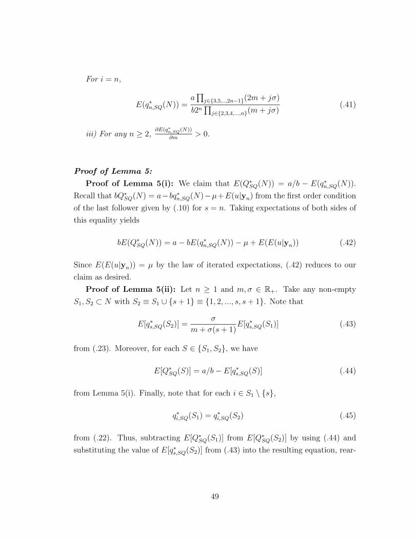
For i = n,
E(q∗n,SQ(N)) =a∏
j∈{3,5,..,2n−1}(2m+ jσ)
b2n∏
j∈{2,3,4,...,n}(m+ jσ)(.41)
iii) For any n ≥ 2,∂E(q∗n,SQ(N))
∂m> 0.
Proof of Lemma 5:
Proof of Lemma 5(i): We claim that E(Q∗SQ(N)) = a/b − E(q∗n,SQ(N)).
Recall that bQ∗SQ(N) = a−bq∗n,SQ(N)−µ+E(u|yn) from the first order condition
of the last follower given by (.10) for s = n. Taking expectations of both sides of
this equality yields
bE(Q∗SQ(N)) = a− bE(q∗n,SQ(N))− µ+ E(E(u|yn)) (.42)
Since E(E(u|yn)) = µ by the law of iterated expectations, (.42) reduces to our
claim as desired.
Proof of Lemma 5(ii): Let n ≥ 1 and m,σ ∈ R+. Take any non-empty
S1, S2 ⊂ N with S2 ≡ S1 ∪ {s+ 1} ≡ {1, 2, ..., s, s+ 1}. Note that
E[q∗s,SQ(S2)] =σ
m+ σ(s+ 1)E[q∗s,SQ(S1)] (.43)
from (.23). Moreover, for each S ∈ {S1, S2}, we have
E[Q∗SQ(S)] = a/b− E[q∗s,SQ(S)] (.44)
from Lemma 5(i). Finally, note that for each i ∈ S1 \ {s},
q∗i,SQ(S1) = q∗i,SQ(S2) (.45)
from (.22). Thus, subtracting E[Q∗SQ(S1)] from E[Q∗SQ(S2)] by using (.44) and
substituting the value of E[q∗s,SQ(S2)] from (.43) into the resulting equation, rear-
49
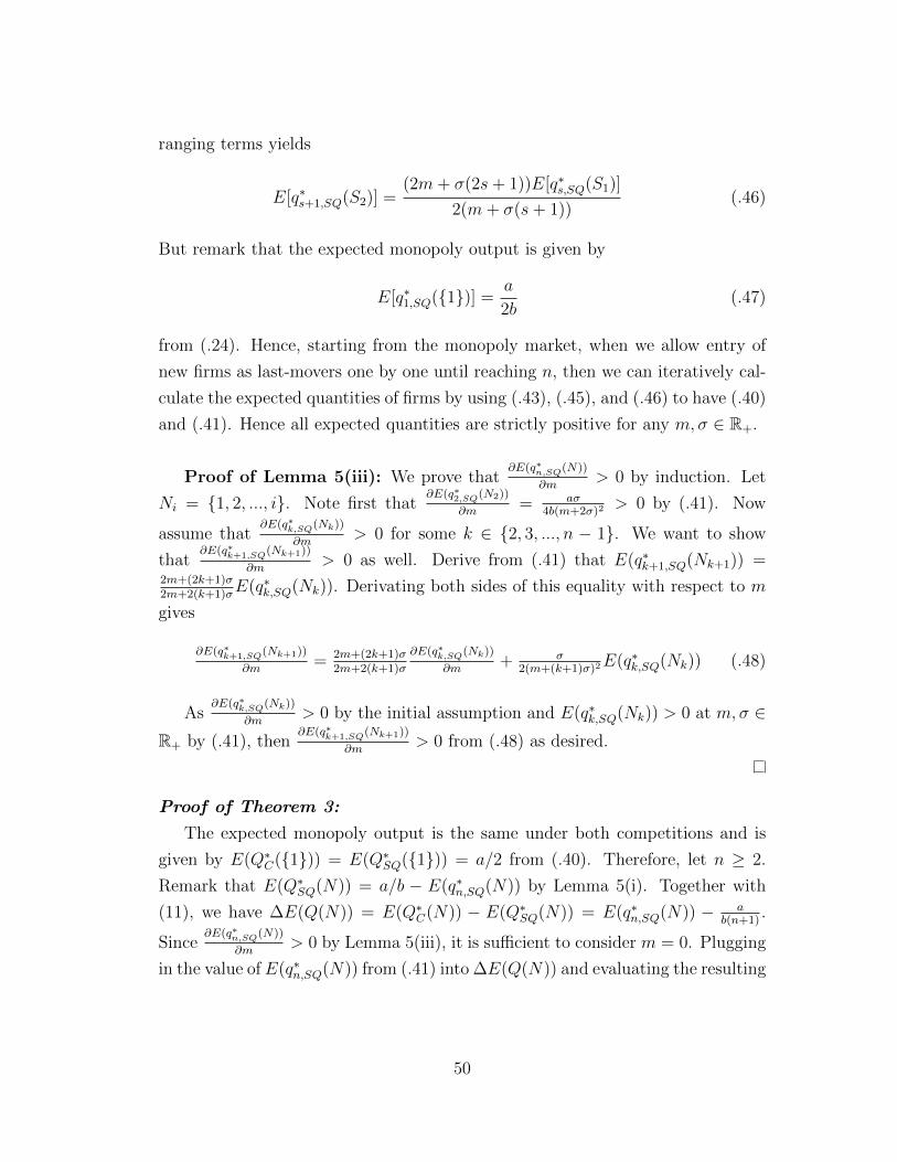
ranging terms yields
E[q∗s+1,SQ(S2)] =(2m+ σ(2s+ 1))E[q∗s,SQ(S1)]
2(m+ σ(s+ 1))(.46)
But remark that the expected monopoly output is given by
E[q∗1,SQ({1})] =a
2b(.47)
from (.24). Hence, starting from the monopoly market, when we allow entry of
new firms as last-movers one by one until reaching n, then we can iteratively cal-
culate the expected quantities of firms by using (.43), (.45), and (.46) to have (.40)
and (.41). Hence all expected quantities are strictly positive for any m,σ ∈ R+.
Proof of Lemma 5(iii): We prove that∂E(q∗n,SQ(N))
∂m> 0 by induction. Let
Ni = {1, 2, ..., i}. Note first that∂E(q∗2,SQ(N2))
∂m= aσ
4b(m+2σ)2> 0 by (.41). Now
assume that∂E(q∗k,SQ(Nk))
∂m> 0 for some k ∈ {2, 3, ..., n − 1}. We want to show
that∂E(q∗k+1,SQ(Nk+1))
∂m> 0 as well. Derive from (.41) that E(q∗k+1,SQ(Nk+1)) =
2m+(2k+1)σ2m+2(k+1)σ
E(q∗k,SQ(Nk)). Derivating both sides of this equality with respect to m
gives
∂E(q∗k+1,SQ(Nk+1))
∂m= 2m+(2k+1)σ
2m+2(k+1)σ
∂E(q∗k,SQ(Nk))
∂m+ σ
2(m+(k+1)σ)2E(q∗k,SQ(Nk)) (.48)
As∂E(q∗k,SQ(Nk))
∂m> 0 by the initial assumption and E(q∗k,SQ(Nk)) > 0 at m,σ ∈
R+ by (.41), then∂E(q∗k+1,SQ(Nk+1))
∂m> 0 from (.48) as desired.
Proof of Theorem 3:
The expected monopoly output is the same under both competitions and is
given by E(Q∗C({1})) = E(Q∗SQ({1})) = a/2 from (.40). Therefore, let n ≥ 2.
Remark that E(Q∗SQ(N)) = a/b − E(q∗n,SQ(N)) by Lemma 5(i). Together with
(11), we have ∆E(Q(N)) = E(Q∗C(N)) − E(Q∗SQ(N)) = E(q∗n,SQ(N)) − ab(n+1)
.
Since∂E(q∗n,SQ(N))
∂m> 0 by Lemma 5(iii), it is sufficient to consider m = 0. Plugging
in the value of E(q∗n,SQ(N)) from (.41) into ∆E(Q(N)) and evaluating the resulting
50
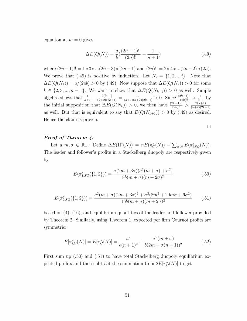
equation at m = 0 gives
∆E(Q(N)) =a
b((2n− 1)!!
(2n)!!− 1
n+ 1) (.49)
where (2n− 1)!! = 1 ∗ 3 ∗ ...(2n− 3) ∗ (2n− 1) and (2n)!! = 2 ∗ 4 ∗ ...(2n− 2) ∗ (2n).
We prove that (.49) is positive by induction. Let Ni = {1, 2, .., i}. Note that
∆E(Q(N2)) = a/(24b) > 0 by (.49). Now suppose that ∆E(Q(Nk)) > 0 for some
k ∈ {2, 3, ..., n − 1}. We want to show that ∆E(Q(Nk+1)) > 0 as well. Simple
algebra shows that 1k+1− 2(k+1)
(k+2)(2k+1)= k
(k+1)(k+2)(2k+1)> 0. Since (2k−1)!!
(2k)!!> 1
k+1by
the initial supposition that ∆E(Q(Nk)) > 0, we then have (2k−1)!!(2k)!!
> 2(k+1)(k+2)(2k+1)
as well. But that is equivalent to say that E(Q(Nk+1)) > 0 by (.49) as desired.
Hence the claim is proven.
Proof of Theorem 4:
Let a,m, σ ∈ R+. Define ∆E(Π∗(N)) = nE(π∗C(N)) −∑
i∈N E(π∗i,SQ(N)).
The leader and follower’s profits in a Stackelberg duopoly are respectively given
by
E(π∗1,SQ({1, 2})) =σ(2m+ 3σ)(a2(m+ σ) + σ2)
8b(m+ σ)(m+ 2σ)2(.50)
E(π∗2,SQ({1, 2})) =a2(m+ σ)(2m+ 3σ)2 + σ2(8m2 + 20mσ + 9σ2)
16b(m+ σ)(m+ 2σ)2(.51)
based on (4), (16), and equilibrium quantities of the leader and follower provided
by Theorem 2. Similarly, using Theorem 1, expected per firm Cournot profits are
symmetric:
E[π∗i,C(N)] = E[π∗C(N)] =a2
b(n+ 1)2+
σ2(m+ σ)
b(2m+ σ(n+ 1))2(.52)
First sum up (.50) and (.51) to have total Stackelberg duopoly equilibrium ex-
pected profits and then subtract the summation from 2E[π∗C(N)] to get
51
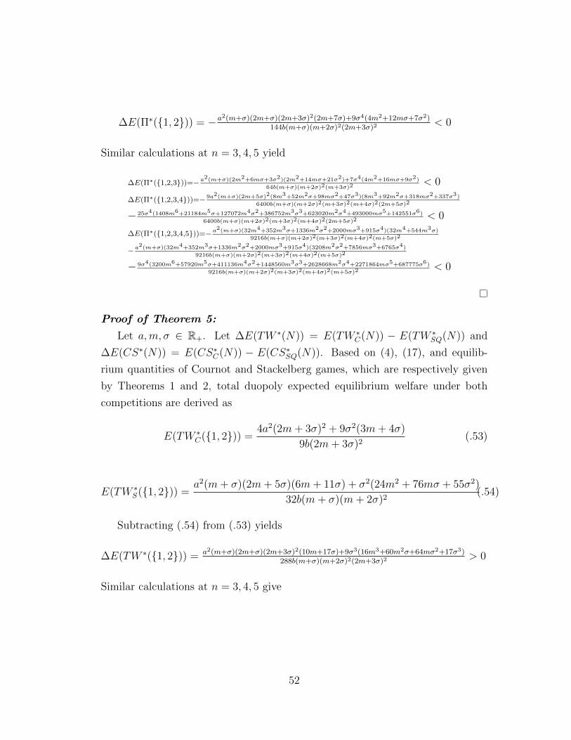
∆E(Π∗({1, 2})) = −a2(m+σ)(2m+σ)(2m+3σ)2(2m+7σ)+9σ4(4m2+12mσ+7σ2)144b(m+σ)(m+2σ)2(2m+3σ)2
< 0
Similar calculations at n = 3, 4, 5 yield
∆E(Π∗({1,2,3}))=−a2(m+σ)(2m2+6mσ+3σ2)(2m2+14mσ+21σ2)+7σ4(4m2+16mσ+9σ2)
64b(m+σ)(m+2σ)2(m+3σ)2< 0
∆E(Π∗({1,2,3,4}))=− 9a2(m+σ)(2m+5σ)2(8m3+52m2σ+98mσ2+47σ3)(8m3+92m2σ+318mσ2+337σ3)
6400b(m+σ)(m+2σ)2(m+3σ)2(m+4σ)2(2m+5σ)2
− 25σ4(1408m6+21184m5σ+127072m4σ2+386752m3σ3+623020m2σ4+493000mσ5+142551σ6)
6400b(m+σ)(m+2σ)2(m+3σ)2(m+4σ)2(2m+5σ)2< 0
∆E(Π∗({1,2,3,4,5}))=−a2(m+σ)(32m4+352m3σ+1336m2σ2+2000mσ3+915σ4)(32m4+544m3σ)
9216b(m+σ)(m+2σ)2(m+3σ)2(m+4σ)2(m+5σ)2
−a2(m+σ)(32m4+352m3σ+1336m2σ2+2000mσ3+915σ4)(3208m2σ2+7856mσ3+6765σ4)
9216b(m+σ)(m+2σ)2(m+3σ)2(m+4σ)2(m+5σ)2
− 9σ4(3200m6+57920m5σ+411136m4σ2+1448560m3σ3+2628668m2σ4+2271864mσ5+687775σ6)
9216b(m+σ)(m+2σ)2(m+3σ)2(m+4σ)2(m+5σ)2< 0
Proof of Theorem 5:
Let a,m, σ ∈ R+. Let ∆E(TW ∗(N)) = E(TW ∗C(N)) − E(TW ∗
SQ(N)) and
∆E(CS∗(N)) = E(CS∗C(N)) − E(CS∗SQ(N)). Based on (4), (17), and equilib-
rium quantities of Cournot and Stackelberg games, which are respectively given
by Theorems 1 and 2, total duopoly expected equilibrium welfare under both
competitions are derived as
E(TW ∗C({1, 2})) =
4a2(2m+ 3σ)2 + 9σ2(3m+ 4σ)
9b(2m+ 3σ)2(.53)
E(TW ∗S({1, 2})) =
a2(m+ σ)(2m+ 5σ)(6m+ 11σ) + σ2(24m2 + 76mσ + 55σ2)
32b(m+ σ)(m+ 2σ)2(.54)
Subtracting (.54) from (.53) yields
∆E(TW ∗({1, 2})) = a2(m+σ)(2m+σ)(2m+3σ)2(10m+17σ)+9σ3(16m3+60m2σ+64mσ2+17σ3)288b(m+σ)(m+2σ)2(2m+3σ)2
> 0
Similar calculations at n = 3, 4, 5 give
52
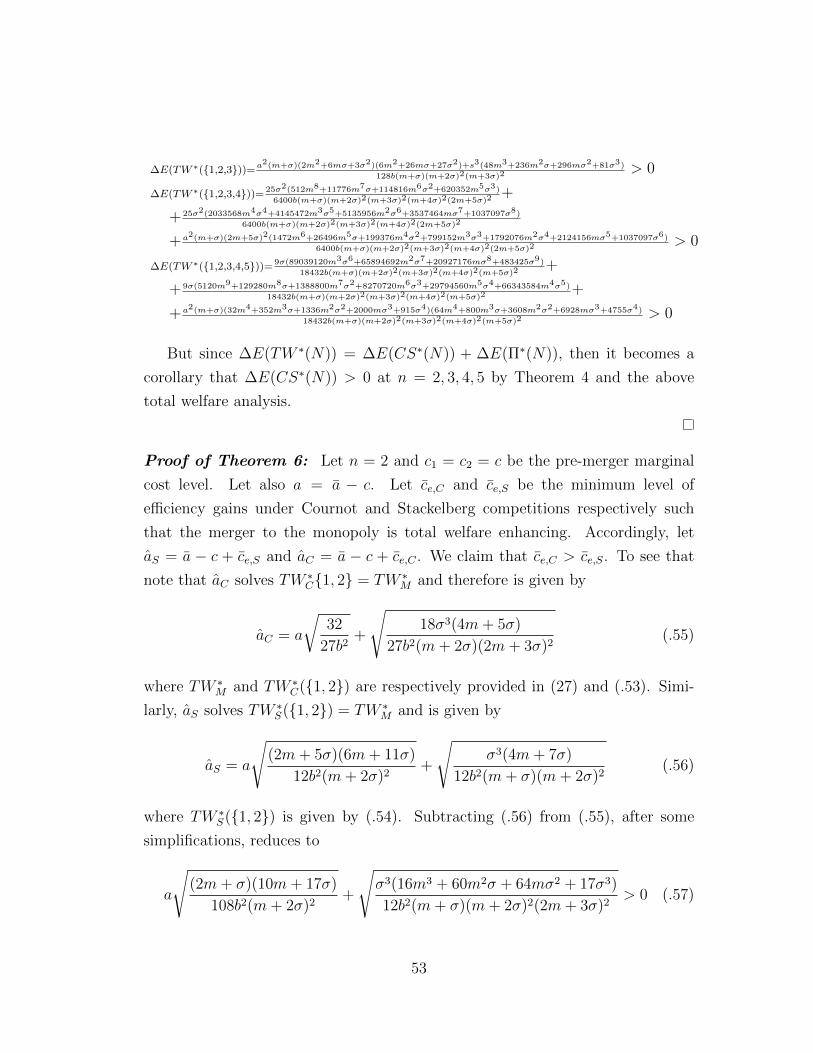
∆E(TW ∗({1,2,3}))=a2(m+σ)(2m2+6mσ+3σ2)(6m2+26mσ+27σ2)+s3(48m3+236m2σ+296mσ2+81σ3)
128b(m+σ)(m+2σ)2(m+3σ)2> 0
∆E(TW ∗({1,2,3,4}))= 25σ2(512m8+11776m7σ+114816m6σ2+620352m5σ3)
6400b(m+σ)(m+2σ)2(m+3σ)2(m+4σ)2(2m+5σ)2+
+ 25σ2(2033568m4σ4+4145472m3σ5+5135956m2σ6+3537464mσ7+1037097σ8)
6400b(m+σ)(m+2σ)2(m+3σ)2(m+4σ)2(2m+5σ)2
+a2(m+σ)(2m+5σ)2(1472m6+26496m5σ+199376m4σ2+799152m3σ3+1792076m2σ4+2124156mσ5+1037097σ6)
6400b(m+σ)(m+2σ)2(m+3σ)2(m+4σ)2(2m+5σ)2> 0
∆E(TW ∗({1,2,3,4,5}))= 9σ(89039120m3σ6+65894692m2σ7+20927176mσ8+483425σ9)
18432b(m+σ)(m+2σ)2(m+3σ)2(m+4σ)2(m+5σ)2+
+ 9σ(5120m9+129280m8σ+1388800m7σ2+8270720m6σ3+29794560m5σ4+66343584m4σ5)
18432b(m+σ)(m+2σ)2(m+3σ)2(m+4σ)2(m+5σ)2+
+a2(m+σ)(32m4+352m3σ+1336m2σ2+2000mσ3+915σ4)(64m4+800m3σ+3608m2σ2+6928mσ3+4755σ4)
18432b(m+σ)(m+2σ)2(m+3σ)2(m+4σ)2(m+5σ)2> 0
But since ∆E(TW ∗(N)) = ∆E(CS∗(N)) + ∆E(Π∗(N)), then it becomes a
corollary that ∆E(CS∗(N)) > 0 at n = 2, 3, 4, 5 by Theorem 4 and the above
total welfare analysis.
Proof of Theorem 6: Let n = 2 and c1 = c2 = c be the pre-merger marginal
cost level. Let also a = a − c. Let ce,C and ce,S be the minimum level of
efficiency gains under Cournot and Stackelberg competitions respectively such
that the merger to the monopoly is total welfare enhancing. Accordingly, let
aS = a − c + ce,S and aC = a − c + ce,C . We claim that ce,C > ce,S. To see that
note that aC solves TW ∗C{1, 2} = TW ∗
M and therefore is given by
aC = a
√32
27b2+
√18σ3(4m+ 5σ)
27b2(m+ 2σ)(2m+ 3σ)2(.55)
where TW ∗M and TW ∗
C({1, 2}) are respectively provided in (27) and (.53). Simi-
larly, aS solves TW ∗S({1, 2}) = TW ∗
M and is given by
aS = a
√(2m+ 5σ)(6m+ 11σ)
12b2(m+ 2σ)2+
√σ3(4m+ 7σ)
12b2(m+ σ)(m+ 2σ)2(.56)
where TW ∗S({1, 2}) is given by (.54). Subtracting (.56) from (.55), after some
simplifications, reduces to
a
√(2m+ σ)(10m+ 17σ)
108b2(m+ 2σ)2+
√σ3(16m3 + 60m2σ + 64mσ2 + 17σ3)
12b2(m+ σ)(m+ 2σ)2(2m+ 3σ)2> 0 (.57)
53
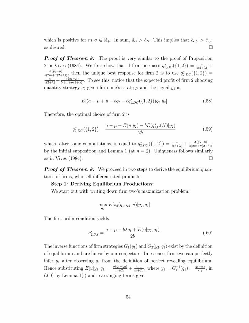
which is positive for m,σ ∈ R+. In sum, aC > aS. This implies that ce,C > ce,S
as desired.
Proof of Theorem 8: The proof is very similar to the proof of Proposition
2 in Vives (1984). We first show that if firm one uses q∗1,DC({1, 2}) = ab(2+λ)
+σ(y1−µ)
b(2m+σ(2+λ)), then the unique best response for firm 2 is to use q∗2,DC({1, 2}) =
ab(2+λ)
+ σ(y2−µ)b(2m+σ(2+λ))
. To see this, notice that the expected profit of firm 2 choosing
quantity strategy q2 given firm one’s strategy and the signal y2 is
E[(a− µ+ u− bq2 − bq∗1,DC({1, 2}))q2|y2] (.58)
Therefore, the optimal choice of firm 2 is
q∗2,DC({1, 2}) =a− µ+ E(u|y2)− bE(q∗1,C(N)|y2)
2b(.59)
which, after some computations, is equal to q∗2,DC({1, 2}) = ab(2+λ)
+ σ(y2−µ)b(2m+σ(2+λ))
by the initial supposition and Lemma 1 (at n = 2). Uniqueness follows similarly
as in Vives (1984).
Proof of Theorem 8: We proceed in two steps to derive the equilibrium quan-
tities of firms, who sell differentiated products.
Step 1: Deriving Equilibrium Productions:
We start out with writing down firm two’s maximization problem:
maxq2
E[π2(q1, q2, u)|y2, q1]
The first-order condition yields
q∗2,DS =a− µ− bλq1 + E(u|y2, q1)
2b(.60)
The inverse functions of firm strategiesG1(y1) andG2(y2, q1) exist by the definition
of equilibrium and are linear by our conjecture. In essence, firm two can perfectly
infer y1 after observing q1 from the definition of perfect revealing equilibrium.
Hence substituting E[u|y2, q1] = σ(y1+y2)m+2σ
+ mµm+2σ
, where y1 = G−11 (q1) = q1−α0
α1, in
(.60) by Lemma 1(i) and rearranging terms give
54

q∗2,DS = G1(y2, q1) =a
2b− σ(α0 + 2α1µ)
2α1(m+ 2σ)+
σy2
2(m+ 2σ)+ (−λ2
+σ
2α1(m+ 2σ))q1
We first substitute q∗2,DS from above in the leader firm’s optimization problem
as
maxq1
E[π1(q1, q∗2,DS, u)|y1] = E[(a− µ+ u− bq1 − bλq∗2,DS)q1|y1] (.61)
After further substituting E[u|y1] = E[y2|y1] = σy1m+σ
+ σµm+σ
in (.61) by Lemma
1, one can solve for α0 and α1 from the first order conditions for the maximization
problem in (.61).
STEP 2: Second Order Conditions for the Differentiated Good Model
Observe first that ∂2E[π2(.)|y2,q1]∂2q2
= −2b < 0 and the second order condition for
the follower is satisfied.
Finally note that ∂2E[π1(.)|y1]∂2q1
= −2b(1 + λβ3) by (.61). As β3 =∂2q∗2∂2q1
=(2−λ)(2m+(2−λ)σ)4(1−λ)m+2(4−3λ)σ
> 0 for any λ ∈ [0, 1] andm,σ ∈ R+ from Theorem 8, ∂2E[π1(.)|y1]
∂2q1<
0. Hence, all second order conditions are satisfied.
Proof of Theorem 9:
i) Let E[∆Q∗D] = E[Q∗DC ] − E[Q∗DS]. By using (4) and equilibrium quanti-
ties of firms in differentiated Cournot and Stackelberg models respectively from
Theorems (7) and (8), it can be shown that
E[∆Q∗D] =aλ(2− λ)(2m+ σ(2− λ))
4b(2 + λ)(2− λ2)(m+ 2σ)(.62)
which is positive for λ ∈ (0, 1] and is equal to zero when λ = 0.
ii) Let a ≥ σ and λ ∈ [0, 1]. We claim that E[∆Π∗D] = E[Π∗DC ]− E[Π∗DS] < 0.
By using (4) and the equilibrium quantities of firms in differentiated Cournot and
Stackelberg models respectively stated in Theorems (7) and (8), it can be shown
that
∂E[∆Π∗D]
∂a= −2a(m(2(1− λ)(4− λ2) + 2λ3) + σ(2− λ)(12− 5λ2))
g< 0 (.63)
55
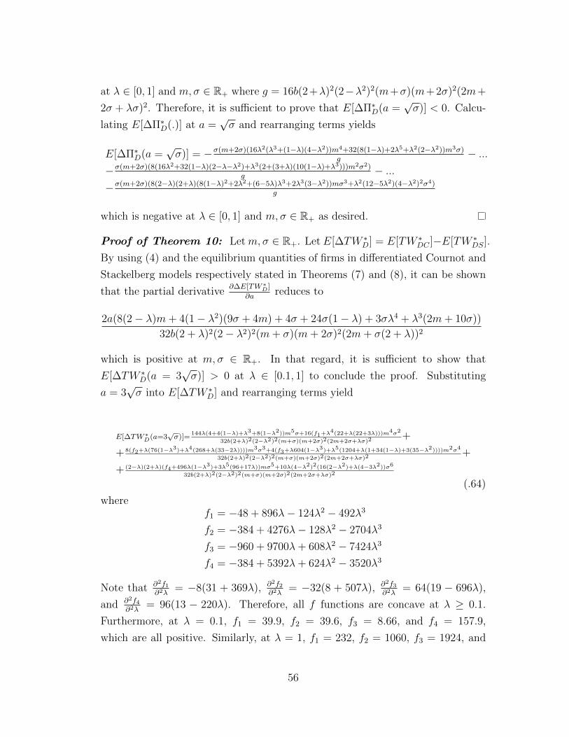
at λ ∈ [0, 1] and m,σ ∈ R+ where g = 16b(2+λ)2(2−λ2)2(m+σ)(m+2σ)2(2m+
2σ + λσ)2. Therefore, it is sufficient to prove that E[∆Π∗D(a =√σ)] < 0. Calcu-
lating E[∆Π∗D(.)] at a =√σ and rearranging terms yields
E[∆Π∗D(a =√σ)] = −σ(m+2σ)(16λ2(λ3+(1−λ)(4−λ2))m4+32(8(1−λ)+2λ5+λ2(2−λ2))m3σ)
g− ...
−σ(m+2σ)(8(16λ2+32(1−λ)(2−λ−λ2)+λ3(2+(3+λ)(10(1−λ)+λ3)))m2σ2)g
− ...−σ(m+2σ)(8(2−λ)(2+λ)(8(1−λ)2+2λ2+(6−5λ)λ3+2λ3(3−λ2))mσ3+λ2(12−5λ2)(4−λ2)2σ4)
g
which is negative at λ ∈ [0, 1] and m,σ ∈ R+ as desired.
Proof of Theorem 10: Letm,σ ∈ R+. LetE[∆TW ∗D] = E[TW ∗
DC ]−E[TW ∗DS].
By using (4) and the equilibrium quantities of firms in differentiated Cournot and
Stackelberg models respectively stated in Theorems (7) and (8), it can be shown
that the partial derivative∂∆E[TW ∗D]
∂areduces to
2a(8(2− λ)m+ 4(1− λ2)(9σ + 4m) + 4σ + 24σ(1− λ) + 3σλ4 + λ3(2m+ 10σ))
32b(2 + λ)2(2− λ2)2(m+ σ)(m+ 2σ)2(2m+ σ(2 + λ))2
which is positive at m,σ ∈ R+. In that regard, it is sufficient to show that
E[∆TW ∗D(a = 3
√σ)] > 0 at λ ∈ [0.1, 1] to conclude the proof. Substituting
a = 3√σ into E[∆TW ∗
D] and rearranging terms yield
E[∆TW ∗D(a=3√σ)]=
144λ(4+4(1−λ)+λ3+8(1−λ2))m5σ+16(f1+λ4(22+λ(22+3λ)))m4σ2
32b(2+λ)2(2−λ2)2(m+σ)(m+2σ)2(2m+2σ+λσ)2+
+ 8(f2+λ(76(1−λ3)+λ4(268+λ(33−2λ))))m3σ3+4(f3+λ604(1−λ
3)+λ5(1204+λ(1+34(1−λ)+3(35−λ2))))m2σ4
32b(2+λ)2(2−λ2)2(m+σ)(m+2σ)2(2m+2σ+λσ)2+
+ (2−λ)(2+λ)(f4+496λ(1−λ3)+3λ5(96+17λ))mσ5+10λ(4−λ2)2(16(2−λ2)+λ(4−3λ2))σ6
32b(2+λ)2(2−λ2)2(m+σ)(m+2σ)2(2m+2σ+λσ)2
(.64)
wheref1 = −48 + 896λ− 124λ2 − 492λ3
f2 = −384 + 4276λ− 128λ2 − 2704λ3
f3 = −960 + 9700λ+ 608λ2 − 7424λ3
f4 = −384 + 5392λ+ 624λ2 − 3520λ3
Note that ∂2f1∂2λ
= −8(31 + 369λ), ∂2f2∂2λ
= −32(8 + 507λ), ∂2f3∂2λ
= 64(19 − 696λ),
and ∂2f4∂2λ
= 96(13 − 220λ). Therefore, all f functions are concave at λ ≥ 0.1.
Furthermore, at λ = 0.1, f1 = 39.9, f2 = 39.6, f3 = 8.66, and f4 = 157.9,
which are all positive. Similarly, at λ = 1, f1 = 232, f2 = 1060, f3 = 1924, and
56
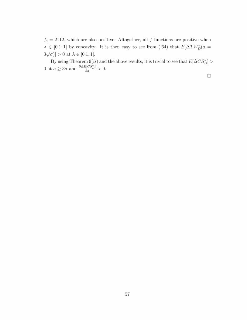
f4 = 2112, which are also positive. Altogether, all f functions are positive when
λ ∈ [0.1, 1] by concavity. It is then easy to see from (.64) that E[∆TW ∗D(a =
3√σ)] > 0 at λ ∈ [0.1, 1].
By using Theorem 9(ii) and the above results, it is trivial to see thatE[∆CS∗D] >
0 at a ≥ 3σ and∂∆E[CS∗D]
∂a> 0.
57
References
[1] ALBAEK, S. (1990), “Stackelberg Leadership as a Natural Solution UnderCost Uncertainty”, The Journal of Industrial Economics, 38, No. 3., 335-347.
[2] AMIR, R. and I. GRILO (1999), “Stackelberg versus Cournot Equilibrium”,Games and Economic Behaviour, 26, 1-21.
[3] ANDERSON, S. P. and M. ENGERS (1992), “Stackelberg versus CournotOligopoly Equilibrium”, International Journal of Industrial Organization, 10,27-135.
[4] BAGWELL, K. (1995), “Commitment and Observability in Games”, Gamesand Economic Behaviour, 8, 271-280.
[5] BOYER, M. and M. MOREAUX (1987), “On Stackelberg Equilibria withDifferentiated Products: The Critical Role of the Strategy Space”, Journal ofIndustrial Economics, 36, 217-230.
[6] CLARKE, R. N. (1983), “Collusion and the Incentives for Information Shar-ing”, Bell Journal of Economics, 14, No. 2., 383-394.
[7] COURNOT, A. (1838), “Recherches sur les Principes Mathematiques de laTheorie des Richesses”, Paris: Hachette.
[8] DAUGHETY, F. A. (1990), “Beneficial Concentration”, American EconomicReview, 80, No. 5., 1231-1237.
[9] DEGROOT, M. H. (1970), “Optimal Statistical Decisions”, Chapter 9,McGraw-Hill, New York.
[10] ERICSON, W. A. (1969), “A Note on the Posterior Mean of a PopulationMean”, Journal of the Royal Statistical Society, 31, 332-334.
[11] GAL-OR, E. (1987), “First-mover Disadvantages with Private Information”,Review of Economic Studies, 54, 279-292.
[12] GAL-OR, E., T. GEYLANI, and J. A. DUKES (2008), “Information Sharingin a Channel with Partially Informed Retailers”, Marketing Science, 27, No4, 642-658.
[13] GAL-OR, E., T. GEYLANI, and J. A. DUKES (2011), “Who Benefits fromBilateral Information Exchange in a Retail Channel”, Economics Letters, 112,210-212.
58
[14] GUTH, W., G. KIRCHSTEIGER, and K. RITZBERGER (1998), “Imper-fectly Observable Commitments in n−Player Games,” Games and EconomicBehaviour, 23, 54-74.
[15] HACKBARTH, D. and MIAO J. (2012), “The Dynamics of Mergers andAcquisitions in Oligopolistic Industries” Journal of Economic Dynamics &Control, 36, 585-609.
[16] KADIYALI, V., K. SUDHIR, and R. V. RAO (2001), “Structural Analysisof Competitive Behavior: New Empirical Industrial Organization Methods inMarketing,” International Journal of Research in Marketing, 18, 161-186.
[17] KUHN K. and X. VIVES (1995), “Information Exchanges Among Firms andTheir Impact on Competition”, Luxembourg: Office for Official Publicationsof the European Communities, ISBN 92-826-9705-3.
[18] JANSSEN, C. W. M. and E. MAASLAND (1997), “On the Uniqune D1Equilibrium in the Stackelberg Model with Asymmetric Information,” CentERfor Economic Research, Tilburg University, Working Paper.
[19] LI, L. (1985), “Cournot Oligopoly with Information Sharing”, The RANDJournal of Economics, 16, 4, 521-536.
[20] LIU, Z. (2005), “Stackelberg Leadership with Demand Uncertainty”, Man-agerial and Decision Economics, 26, 345-350.
[21] LOPEZ, A. R., A. M. AZZAM, and C. LIRON-ESPANA (2002), “MarketPower and/or Efficiency: A Structural Approach”, Review of Industrial Orga-nization, 20, 115-126.
[22] MAGGI, G. (1999), “The Value of Commitment with Imperfect Observabilityand Private Information”, Rand Journal of Economics, 30, 4, 555-574.
[23] MAILATH, G. (1993), “Endogeneous Sequencing of Firm Decisions”, Journalof Economic Theory, 59, 169-182.
[24] MILGROM, P. and J. ROBERTS (1982), “Limit Pricing and Entry underIncomplete Information: An Equilibrium Analysis”, Econometrica, 50, 2, 443-459.
[25] MORGAN, J. and F. VARDY (2007), “The Value of Commitment in Con-tests and Tournaments When Observation is Costly”, Games and EconomicBehaviour, 60, 326-338.
[26] NEWMARK M. C. (2004), “Price-Concentration Studies: There You GoAgain”, Prepared for the DOJ/FTC Merger Workshop, “Concentration andMarket Shares” Panel
59
[27] OKUGUCHI, K. (1999), “Cournot and Stackelberg Duopolies Revisited”,Japanese of Economic Review, 50, No. 3.
[28] RAJU, S. J. and A. ROY (2000), “Market Information and Firm Perfor-mance”, Management Science, 46, 8, 1075-1084.
[29] SHINKAI, T. (2000), “Second Mover Disadvantages in a Three-Player Stack-elberg Game with Private Information”, Journal of Economic Theory, 90,293-304.
[30] SPENCE, M. (1973), “Job Market Signaling”, Quarterly Journal of Eco-nomics, 83, 3, 355-374.
[31] TIROLE, J. (1995), “The Theory of Industrial Organization”, Eighth print-ing, Chapter 11, 450-453.
[32] VARDY, F. (2004), “The Value of Commitment in Stackelberg Games withObservation Costs”, Games and Economic Behaviour, 49, 374-400.
[33] VAN DAMME, E. and S. HURKENS (1997), “Games with Imperfectly Ob-servable Commitment”, Games and Economic Behaviour, 21, 282-308.
[34] VIVES, X. (1984), “Duopoly Information Equilibrium”, Journal of EconomicTheory, 34, 71-94.
[35] VIVES, X. (1999), “Oligopoly Pricing: Old Ideas and New Tools”, MIT PressBooks, The MIT Press, edition 1, vol. 1.
[36] VIVES, X. (2011), “Strategic Supply Function Competition With PrivateInformation”, Econometrica, 79, No. 6., 1919-1966.
[37] von STACKELBERG, H. (1934), “Marktform und Gleichgewicht”, Vienna:Springer.
60
Recommended