Pertanika J. Sci. & Techno!. 3(2): 271-283 (1995)ISSN:OI28-7680
© Penerbit Universiti Pertanian Malaysia
Stability Conditions for an AlternatedGrid in Space and Time
Alejandro L. Camerlengo and Monica Ines DemmlerFaculty of Fisheries and Marine Science
Universiti Pertanian MalaysiaMengabang Telipot, 21030 Kuala Terengganu, Malaysia
Received 28 October 1994
ABSTRAKKeadaan kestabilan kekisi bertindan di dalam ruang dan masa telah dirumuskan.Grid yang sedang dirujuk ini, dikenali sebagai grid Eliassen (Eliassen 1956).Telah ditunjukkan bahawa keadaan kestabilan di dalam persamaan gelombangperairan cetek unruk kekisi jenis ini adalah keadaan kestabilan yang serupauntuk grid tidak bertindak kekisi Arakawa's B dan C. Bila melaksanakan skim'leapfrog' di dalam grid bertindan mengikut ruang dan masa, didapati tiadamempunyai mod pengiraan. Tiada pengiraan purata diperlukan untuk mengiraistilah Coriolis (gelombang graviti) sebagaimana yang diperlukan di dalam gridArakawa's B dan C. Di samping itu, penggunaan grid Eliassen menjimatkanseparuh masa pengiraan yang diperlukan dalam grid Arakawa's B atau C(Mesinger and Arakawa 1976). Oleh itu, adalah lebih menguntungkan denganmengguna grid silih berganti di dalam ruang dan masa.
ABSTRACTThe stability conditions of a staggered lattice in space and time are derived.The grid used is known as the Eliassen grid (Eliassen 1956). It is shown that thestability conditions of the shallow water wave equations, for this type of lattice,have essentially the same stability condition as the unstaggered grid andArakawa's B and C lattice. Upon implementation of a leapfrog scheme in astaggered grid in space and time, there will be no computational modes. Nosmoothing is needed to compute the Coriolis (gravity wave) terms as requiredin Arakawa's C (B) grid. Furthermore, the usage of an Eliassen grid halves thecomputation time required in Arawaka's B or C grid (Mesinger and Arakawa1976). Therefore, there are fundamental advantages for the usage of analternated grid in space and time.
Keywords: numerical stability, lattice, inertia - gravity waves, leapfrog
INTRODUCTION
Camerlengo and 0' Brien (1980), using a staggered grid in space and time(Fig. 1), tested different sets of open boundary conditions for rotating(geophysical) fluids. In computing (with this type of grid) the Coriolisterms, quite an amount of averaging is avoided compared to the computation of these same terms by the widely-used Arakawa's C lattice.

t
Alejandro L. Camerlengo & Monica Ines Demmler
u
v
u
u
v
n6 t ~h V:.L..-_-----..:h-=--_-..:/
v
(n -1)6t ~_--=:;L--__..e.....-_----=-U
Fig. J. The analysed staggered lattice in space and time
x
Upon using a leapfrog scheme, two solutions per time step areobtained. The first one (the physical mode) resembles the true (real)solution. The second one (the computational mode) is a spurious one. Ittravels in an opposite direction to the physical mode. Furthermore, itsamplitude changes sign at every time level (Haltiner and Williams 1980).
To eliminate the computational mode, a forward (or backward) timescheme is usually implemented (in the numerical integration) at every N(odd) time step. The time differencing scheme most commonly used inmeteorology and physical oceanography modelling is the Matsuno scheme(Matsuno 1966). However, (due to the fact that the computational modewill reappear as soon as the leapfrog scheme is used) the implementationof the first order time differencing scheme does not seem to be the idealsolution. A more radical approach needs to be taken.
In using a staggered grid in time and space, the computational modeis avoided, as the variables at alternate time levels are missing.
The aim of this study is to gain some understanding of the numericalstability of the Eliassen grid. Following O'Brien (1986), stability analysis ofa sequence of problems, for the Eliassen grid, leading to the linear shallowwater wave equations, is considered. A series of analytical studies isconducted. The linear stability technique developed by von Neumann isused (Charney et al. 1950).
272 Pertanika J. Sci. & Techno!. Vo!. 3 No.2, 1995

Stability Condition for an Alternated Grid in Space and Time
NUMERICAL STABILITY PROBLEM
The linear stability condition of the finite difference schemes is determined by the phase speed of the gravity waves, C, i.e., by the velocity of thefastest travelling waves. The general stability condition is :
C !J..t :s:; 0 (1)~
Stability Analysis for One-dimensional Gravity WaveLet us consider the following set of partial differential equations:
Ju Db- =-g-dt Jx
(1)
Db Ju- =-H-dt Jx
where g represents the earth's gravity; H, the mean sea-level depth; u andv, the velocity components in the x (east-west) and y (north-south)directions, respectively; and h, the free surface elevation.
A second order, centred, in space and time finite difference scheme,is considered (Fig. 2). Primed quantities represent variables at odd timelevels. We obtain:
U'~~/ =U'~~/ -gyx (h~=!,,-h~_l,I)
h "'+! h,n-l H ( n n)m,l+! = m,l+! -Yx Um+1,1=1 -um-l,l+!
(2)
where "Ix is equal to /),t/ /),x; the superscript n, denotes the time level; thesubscripts (m,T), the mesh of discrete points in the x and y directions,
respectively; /),x and /),y, the grid size between grid points in the x and y
directions, respectively; and /),t, the time step increment.
We define:
C2 =gH,
e =Il/),x,
(J = v/),Y,
Pertanika J. Sci. & Techno!. Vo!. 3 No.2, 1995 273

Alejandro L. Camerlengo & Monica Ines Dernmler
v U'hv U'hv U' , ,
h',
h' U,
h'U,V v
v u' h V,U' h V,U,
h',
h' U,V,
h'u,v
by D.X
V, u' h V,U' h V,U
(-1
f-2m-2 m-1 m
x )
Fig. 2. Space representation of the altemated grid in space and time.Primed quantities represent variables at odd time levels
where J-L and v are the latitudinal and longitudinal wave numbers, respectively. Let us assume that:
P~,l = Pn exp (i J1 mLix) exp (i v ILiy) (3)
where P = (u, h). It is convenient to drop the primes. If we substituteequation (3) in (2), we obtain:
Un+ 1 =Un- 1-gYx(2isin8)hn
hn+ 1 =hn-1-Hyx (2isin8)u n(4)
If an amplification factor, Z, exists such that
PIl+2 = Z Pn
(5)
equation (4) can be rewritten as:
L, un + L 2 h n =0
L1 hn + L3 Un =0(6)
274 Pertanika J. Sci. & Techno!. Va!. 3 No.2, 1995

Stability Condition for an Alternated Grid in Space and Time
The operators Lt , L2
, and L3
are defined as:
Zl/2 _ Z-1/2
2 g Yx
2 H Yx
sin esin e
For the system (6) to have a determinate solution:
=0
The second order equation for Z is:
(7)
(8)
If the term [1- (1- 2C2 Y; sin2e) 2] is positive, then the amplification
factor will be equal to one. Thus, the stability analysis shows that thechosen finite difference scheme is neutral. Namely that IZ 1=1. Thisinstance will hold true if, and only if:
That is:
which is the classical Courant-Friedrichs-Levy (CF) condition for computational stability.
Stability Conditions for the Inertial-gravity WavesWe consider the following system of partial differential equations:
Pertanika J. Sci. & Techno\. Vol. 3 No.2, 1995 275

auat
Alejandro L. Camerlengo & Monica Ines Demmler
ahf Y - g ax
ay-=-fuat (9)
ahat
au- H ax
We assume that:
Q~,l = Q n exp (i ).l mL1x) exp (i v L1y)
where Q = (u, Y, h) and an amplification factor, Z, exists such that:
(10)
A leapfrog in time and second order space difference scheme IS
considered. We obtain:
u n+ 1 un-l + 2 L1t f v n - 2
v n+ 1 vn-l 2 L1t f un
hn+! hn- 1 - 2 i H Yx sin 8
Equation (11) may be rewritten as:
L[ un L4 Yn + L2 h n = 0
L1 Yn + L4 Un 0
L! h n + L3 un 0
g Yx sin e hn
un
(11)
where L4 = 2 f L1t.
Following the same procedure as in the previous section, yields:
Z = [1 - 2 (fL1t)2 - 2 C2 y~ sin2 e] ±
i [1 - (1 - 2 (Mt)2 - 2 C2 y~ sin2 ef]I/2(12)
276 Pertanika 1. Sci. & Techno!. Vol. 3 No.2, 1995

Stability Condition for an Alternated Grid in Space and Time
If the term under the radical sign is positive, the stability analysis showsthat the absolute value of the amplification factor is equal to one. We willhave a neutral stability condition. This will require that:
(13)
That is
Adamec and O'Brien (1978), in their reduced-gravity model, used a~ t of the order 104sec. At mid=latitudes (f "" 10-4 sec-1). the productf ~t could be of order one. Thus, the stability condition (for reducedgravity models) could be easily violated, if caution is not taken.
However, for barotropic (vertically integrated) models, ~t varies from100 to 600 sec. The product (f ~t? could be of the order 10-3. Therefore,the term (f ~t)2 does not represent a serious problem, since it is verysmall.
Stability Conditions for 2D FlowConsider the linear shallow water wave equations at a constant latitude,i.e., f = constant. We will have:
au ah- f v - g -at ax
av- f u -
ah(14)- g-
at ay
ah _ H (au + av)- =at ax ay
Upon using, as in the two previous sections, a centred in space andtime difference scheme yields:
un+1 Un_I + 2 t.t f v - 2 g Yx sin 8 hnn
vn+1 vn- 1 2 t.t f u - 2 g Yy sin cr hn (15)n
hn+1 hn+1 2 H i [Yx sin 8 un + Yy sin cr vn]
where 'Y is equal to ~t/~y.y
Pertanika J. Sci. & Techno!. Vo!. 3 No.2, 1995 277

Alejandro L. Camerlengo & Monica Ines Demmler
The above system of equations, (15), may be rewritten as:
L1 un L4 vn + L2 hn 0
L1 Y n + L4 Un + LS hn 0
L, hn + L3 Un + L6 Y n 0
where
LS 2 g Yy sin ()
L6 2 H Yy sin ()
(16)
For the set of equations (16) to have a unique solution, it follows that:
Following the same procedure as in the previous cases, yields:
Z2 - 2 X Z + 1 = 0
where
X = 1 - [2 (f~t)2 + 2C2 (y~ sin2 e + y; sin2 cr)]
Neutral stability conditions will be obtained if:
(17)
(18)
(19)
Several cases are considered.
a) For Lx = 2~x and Ly = 2~y, i.e. e = cr = n, where Lx and Ly are
the wavelengths in the x and y directions, respectively, we obtain:
(f ~t)2
~ 1 for stability
b) For Lx =4L1x and Ly = 4L\y, i.e., () =() =n / 2, yields:
(20)
(21)
278 Pertanika J. Sci. & Techno!. Vo!. 3 No.2, J995

Stability Condition for an Alternated Grid in Space and Time
If ~x = ~y = ~ the following relation holds:
(22)
Close to the equator, f z 0, we obtain:
(23)
The same stability condition is obtained for the two-dimensionalunstaggered grid case.
c) For Lx =8 L1x and L y =8 D..y, we will have:
(24)
If D..x =D..y =D.., it may be obtained:
(25)
Therefore,
(26)
Stability condition is larger than in the two previous cases. This is natural
since this stability condition is for the 8 D..x wave.
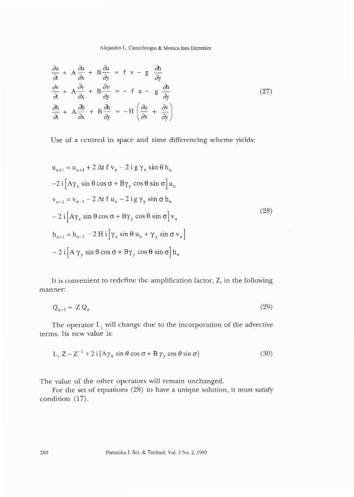
Stability Condition for a 2D Gravity Wave with Advection.We consider the following set of partial differential equations:
Pertanika J. Sci. & Techno!. Vol. 3 No.2, 1995 279
Alejandro L. Camerlengo & Monica Ines Demmler
Ou OuB
Ouf
em-+ A- + v - g -at dx dy dy
iJv iJv B Jv - f u - em(27)-+ A-+ g-
at dx dy dy
emA
em Bem
-H(~ + ~)-+ +at dx dy
Use of a centred in space and time differencing scheme yields:
u n+ 1 = U n+ 1 + 2 .11t f vn - 2 i g Yx sin 8 hn
-2 i [Ay x sin 8 cos <J + By y cos 8 sin cr] un
Vn+l = Vn-l - 2 .11t f Un - 2 i g Yy sin cr hn
-2i[Ayx sin8cos<J+By y cos8sincr]vn
h n+ 1 =hn- 1 - 2 H i [yx sin 8 un + Yy sin <J vn]
- 2 i[A Yy sin 8 cos cr + By y cos e sin cr] hn
(28)
It is convenient to redefine the amplification factor, Z, in the followingmanner:
(29)
The operator L1
will change due to the incorporation of the advectiveterms. Its new value is:
L1 Z - Z-l + 2 i [Ayx sin () cos 0"+ B yy cos () sin 0"] (30)
The value of the other operators will remain unchanged.For the set of equations (28) to have a unique solution, it must satisfy
condition (17).
280 Pertanika J. Sci. & Techno!. Vo!. 3 No.2, 1995

Stability Condition for an Alternated Grid in Space and Time
Upon substitution of the operators LI' , L6
in equation (17), andafter some mathematical manipulations, a second and a fourth orderequation will be obtained. The second order equation yields:
Z2 + 2 i F Z -1 =0
where:
F =A Yx sin ecos cr + Byy cos esin cr
(31)
(32)
Equation (31) represents the advection equation. Following the sameprocedures as in previous sections, a neutral stability solution is obtained if:
In other words:
IA Yx sine cos CY + B Yy cos esin CY! ~ 1
On the other hand, the fourth order equation is:
Z4 + 4 i P Z3 - 2 G Z2 - 4 i P Z + 1= 0
where
(33)
(34)
(35)
The reader can verifY that equation (34) may be factorized in two parts.Namely, that:
[Z2 + (2 i P + (2 G - 4 p2
- 2t 2 ) Z - 1] *
[Z2 + (2 i P- (2 G- 4p2 - 2t 2 )Z -1] = 0(36)
Using either of the quadratic factors, after some algebraic manipulations, a general condition for stability is obtained:
Pertanika J. Sci. & Techno!. Vo!. 3 No.2, 1995 281

Alejandro L. Camerlengo & Monica Ines Demrnler
(37)
For Lx = 2Lix (4 Lix) and L y = 2~y (4 ~y), results similar to those in sec
tions 3.a and 3.b are obtained;
However, for Lx = 8& and L y = 8 .1y; i.e., () = (J = n / 4; & =.1y =.1;
(2 2)1/2
IAI = IBI; Yx = Yy = y; and lUi = A + B yields:
This can be written as:
(38)
Advective terms are computed over a 4 ~distance. Therefore, thestability condition, due to the advective terms, is twice the value for theunstaggered grid. As expected, the CFL condition for the Coriolis andgravity terms are in perfect agreement with stability condition obtained insection 3.c.
We have conducted a similar stability analysis for variables at even timelevels. The results were identical.
CONCLUSIONIn using a leapfrog scheme in an staggered grid in space and time, there areno computational modes. Furthermore, the excessive smoothing needed tocompute the Coriolis (gravity wave) terms in the C (B) lattice is avoided.
It is shown that the stability conditions for the shallow water waveequations, using an Eliassen grid, are practically the same as for the unstaggered(0' Brien 1986). As expected, the truncation error remains unchanged.
The usage of an Eliassen grid saves by half the computation timerequired either on an Arawaka's B or C grid (Mesinger and Arakawa 1976:53). Furthermore, the computational modes are nonexistent. Therefore,there are fundamental advantages in the usage of an alternated grid inspace and time.
282 Pertanika J. Sci. & Techno!. Vol. 3 No.2, 1995

Stability Condition for an Alternated Grid in Space and Time
ACKNOWLEDGMENTS
The study was supported by Universiti Pertanian Malaysia under ContractNo. 50212-94-05. The authors gratefully acnowledge this support. Comments made by reviewers contribute to improving this paper. We wouldlike to extend to them our gratitude. The authors acknowledge thepioneering work of Dr. JJ. 0' Brien in the area of numerical stability.
REFERENCESADAMEC, D and JJ. O'BRIEN. 1978. The seasonal upwelling in the Gulf of Guinea due to
remote forcing. JlYUmal ofPhysical Oceanography 8: 1050-1060.
CAMERLENGO, A. L. and JJ. 0' BRIEN. 1980. Open boundary condition in rotating fluids.Journal of Computational Physics 35: 12-35.
CHARNEY,]. G., FJORTOFf, and]. VON NEUMANN. 1950. Numerical integration ofthe barotropicvorticity equations. Tellus 2: 237-254.
EUASSEN, A. 1956. A Procedure for Numerical Integration of the Primitive Equations of the Twoparameter Model of the Atmosphere. Dept. of the Meteorology, Univ. of California, LosAngeles, Sci. Rept. 4.
HALTINER, GJ. and R.T. WtLLIAMs. 1980. NumericalPrediction and Dynamic Meteorology . Wiley.
MATSUNO, T. 1966. Numerical integration of the primitive equations by a simulatedbackward difference method. JlYUmal Meteorological SocietyJapan, Ser. 2, 44: 76 - 84.
MESINGER, F. and A. ARAKAWA. 1976. Numerical Methods used in Atmospheric Models. GARPPublications Series, No. 17. Geneva: World Meteorological Organization.
0' BRIEN,].]. 1986. Advanced Physical Oceanographic Numerical Modeling. D. Reidel.
Pertanika J. Sci. & Techno!. Vo!. 3 No.2, 1995 283
Recommended