SphereNet: Learning Spherical Representations for
Detection and Classification in Omnidirectional Images
Benjamin Coors1,3, Alexandru Paul Condurache2,3, and Andreas Geiger1
1 Autonomous Vision Group, MPI for Intelligent Systems and University of Tubingen2 Institute for Signal Processing, University of Lubeck
3 Robert Bosch GmbH
Abstract. Omnidirectional cameras offer great benefits over classical cameras
wherever a wide field of view is essential, such as in virtual reality applications
or in autonomous robots. Unfortunately, standard convolutional neural networks
are not well suited for this scenario as the natural projection surface is a sphere
which cannot be unwrapped to a plane without introducing significant distortions,
particularly in the polar regions. In this work, we present SphereNet, a novel
deep learning framework which encodes invariance against such distortions ex-
plicitly into convolutional neural networks. Towards this goal, SphereNet adapts
the sampling locations of the convolutional filters, effectively reversing distor-
tions, and wraps the filters around the sphere. By building on regular convolu-
tions, SphereNet enables the transfer of existing perspective convolutional neural
network models to the omnidirectional case. We demonstrate the effectiveness of
our method on the tasks of image classification and object detection, exploiting
two newly created semi-synthetic and real-world omnidirectional datasets.
1 Introduction
Over the last years, omnidirectional imaging devices have gained in popularity due to
their wide field of view and their widespread applications ranging from virtual reality
to robotics [10,16,21,27,28]. Today, omnidirectional action cameras are available at an
affordable price and 360◦ viewers are integrated into social media platforms. Given the
growing amount of spherical imagery, there is an increasing interest in computer vision
models which are optimized for this kind of data.
The most popular representation of 360◦ images is the equirectangular projection
where latitude and longitude of the spherical image are mapped to horizontal and ver-
tical grid coordinates, see Figs. 1+2 for an illustration. However, the equirectangular
image representation suffers from heavy distortions in the polar regions which implies
that an object will appear differently depending on its latitudinal position. This presents
a challenge to modern computer vision algorithms, such as convolutional neural net-
works (CNNs) which are the state-of-the-art solution to many computer vision tasks.
While CNNs are capable of learning invariances to common object transformations
and intra-class variations, they would require significantly more parameters, training
samples and training time to learn invariance to these distortions from data. This is un-
desirable as data annotation is time-consuming and annotated omnidirectional datasets

2 Benjamin Coors, Alexandru Paul Condurache, Andreas Geiger
(a) 360◦ Cameras (b) 360◦ Image (c) Regular Kernel (d) SphereNet Kernel
Fig. 1: Overview. (a+b) Capturing images with fisheye or 360◦ action camera results in
images which are best represented on the sphere. (c) Using regular convolutions (e.g.,
with 3 × 3 filter kernels) on the rectified equirectangular representation (see Fig. 2b)
suffers from distortions of the sampling locations (red) close to the poles. (d) In contrast,
our SphereNet kernel exploits projections (red) of the sampling pattern on the tangent
plane (blue), yielding filter outputs which are invariant to latitudinal rotations.
are scarce and smaller in size than those collected for the perspective case. An attrac-
tive alternative is therefore to encode invariance to geometric transformations directly
into a CNN, which has been proven highly efficient in reducing the number of model
parameters as well as the required number of training samples [4, 29].
In this work, we present SphereNet, a novel framework for processing omnidirec-
tional images with convolutional neural networks by encoding distortion invariance into
the architecture of CNNs. SphereNet adjusts the sampling grid locations of the convolu-
tional filters based on the geometry of the spherical image representation, thus avoiding
distortions as illustrated in Figs. 1+2. The SphereNet framework applies to a large num-
ber of projection models including perspective, wide-angle, fisheye and omnidirectional
projection. As SphereNet builds on regular convolutional filters, it naturally enables the
transfer of CNNs between different image representations by adapting the sampling
locations of the convolution kernels. We demonstrate this by training object detectors
on perspective images and transferring them to omnidirectional inputs. We provide ex-
tensive experiments on semi-synthetic as well as real-world datasets which demonstrate
the effectiveness of the proposed approach for image classification and object detection.
In summary, this paper makes the following contributions:
• We introduce SphereNet, a framework for learning spherical image representations
by encoding distortion invariance into convolutional filters. SphereNet retains the
original spherical image connectivity and, by building on regular convolutions, en-
ables the transfer of perspective CNN models to omnidirectional inputs.
• We improve the computational efficiency of SphereNet using an approximately uni-
form sampling of the sphere which avoids oversampling in the polar regions.
• We create two novel semi-synthetic and real-world datasets for object detection in
omnidirectional images.
• We demonstrate improved performance as well as SphereNet’s transfer learning
capabilities on the tasks of image classification and object detection and compare
our results to several state-of-the-art baselines.
SphereNet: Learning Spherical Representations in Omnidirectional Images 3
2 Related Work
There are few deep neural network architectures specifically designed to operate on
omnidirectional inputs. In this section, we review the most related approaches.
Khasanova et al. [14] propose a graph-based approach for omnidirectional image
classification. They represent equirectangular images using a weighted graph, where
each image pixel is a vertex and the weights are designed to minimize the difference
between filter responses at different image locations. This graph structure is processed
by a graph convolutional network, which is invariant to rotations and translations [15].
While a graph representation solves the problem of discontinuities at the borders of an
equirectangular image, graph convolutional networks are limited to small graphs and
image resolutions (50 × 50 pixels in [15]) and have not yet demonstrated recognition
performance comparable to regular CNNs on more challenging datasets. In contrast,
our method builds on regular convolutions, which offer state-of-the-art performance for
many computer vision tasks, while also retaining the spherical image connectivity.
In concurrent work, Cohen et al. [3] propose to use spherical CNNs for classification
and encode rotation equivariance into the network. However, often full rotation invari-
ance is not desirable: similar to regular images, 360◦ images are mostly captured in one
dominant orientation (i.e., it is rare that the camera is flipped upside-down). Incorporat-
ing full rotation invariance in such scenarios reduces discriminative power as evidenced
by our experiments. Furthermore, unlike our work which builds on regular convolutions
and is compatible with modern CNN architectures, it is non-trivial to integrate either
graph or spherical convolutions into network architectures for more complex computer
vision tasks like object detection. In fact, no results beyond image classification are pro-
vided in the literature. In contrast, our framework readily allows for adapting existing
CNN architectures for object detection or other higher-level vision tasks to the omnidi-
rectional case. While currently only few large omnidirectional datasets exist, there are
many trained perspective CNN models available, which our method enables to transfer
to any omnidirectional vision task.
Su et al. [30] propose to process equirectangular images with regular convolutions
by increasing the kernel size towards the polar regions. However, this adaptation of the
convolutional filters is a simplistic approximation of distortions in the equirectangular
representation and implies that weights can only be shared along each row, resulting in
a significant increase in model parameters. Thus, this model is hard to train from scratch
and kernel-wise pre-training against a trained perspective model is required. In contrast,
we retain weight sharing across all rows and columns so that our model can be trained
directly end-to-end. At the same time, our method better approximates the distortions
in equirectangular images and allows for perspective-to-omnidirectional representation
transfer.
One way of mitigating the problem of learning spherical representations are cube
map projections as considered in [19, 22]. Here, the image is mapped to the six faces
of a cube which are considered as image planes of six virtual perspective cameras and
processed with a regular CNN. However, this approach does not remove distortions but
only minimizes their effect. Besides, additional discontinuities at the patch boundaries
are introduced and post-processing may be required to combine the individual outputs
4 Benjamin Coors, Alexandru Paul Condurache, Andreas Geiger
of each patch. We avoid these problems by providing a suitable representation for spher-
ical signals which can be directly trained end-to-end.
Besides works on distortion invariance, several works focus on invariances to geo-
metric transformations such as rotations or flips. Jaderberg et al. [11], introduce a sep-
arate network which learns to predict the parameters of a spatial transformation of an
input feature map. Scattering convolution networks [1,25] use predefined wavelet filters
to encode stable geometric invariants into networks while other recent works encode in-
variances into learned convolutional filters [4, 9, 29, 31]. These works are orthogonal to
the presented framework and can be advantageously combined.
Several recent works also consider adapting the sampling locations of convolutional
networks, either dynamically [5] or statically [12, 18]. Unlike our work, these methods
need to learn the sampling locations during training, which requires additional model
parameters and training steps. In contrast, we take advantage of the geometric properties
of the camera to inject this knowledge explicitly into the network architecture.
3 Method
This section introduces the proposed SphereNet framework. First, we describe the adap-
tation of the sampling pattern to achieve distortion invariance on the surface of the
sphere (Section 3.1). Second, we propose an approximation which uniformly samples
the sphere to improve the computational efficiency of our method (Section 3.2). Finally,
we present details on how to incorporate SphereNet into a classification model (Sec-
tion 3.3) as well as how to perform object detection on spherical inputs (Section 3.4).
3.1 Kernel Sampling Pattern
The central idea of SphereNet is to lift local CNN operations (e.g. convolution, pooling)
from the regular image domain to the sphere surface where fisheye or omnidirectional
images can be represented without distortions. This is achieved by representing the
kernel as a small patch tangent to the sphere as illustrated in Fig. 1d. Our model focuses
on distortion invariance and not rotation invariance, as in practice 360◦ images are
mostly captured in one dominant orientation. Thus, we consider upright patches which
are aligned with the great circles of the sphere.
More formally, let S be the unit sphere with S2 its surface. Every point s = (φ, θ) ∈S2 is uniquely defined by its latitude φ ∈ [−π
2 ,π2 ] and longitude θ ∈ [−π, π]. Let
further Π denote the tangent plane located at sΠ = (φΠ , θΠ). We denote a point on Π
by its coordinates x ∈ R2. The local coordinate system of Π is hereby centered at s and
oriented upright. Let Π0 denote the tangent plane located at s = (0, 0). A point s on
the sphere is related to its tangent plane coordinates x via a gnomonic projection [20].
While the proposed approach is compatible with convolutions of all sizes, in the
following we consider a 3 × 3 kernel, which is most common in state-of-the-art archi-
tectures [8, 26]. We assume that the input image is provided in equirectangular format
which is the de facto standard representation for omnidirectional cameras of all form
factors (e.g. catadioptric, dioptric or polydioptric). In Section 3.2 we consider a more
efficient representation that improves the computational efficiency of our method.

SphereNet: Learning Spherical Representations in Omnidirectional Images 5
(a) Sphere
−3.142 −1.571 0.000 1.571 3.142
longitude θ
−1.57
0.00
1.57
latitudeφ
(b) Equirectangular
Fig. 2: Kernel Sampling Pattern at φ = 0 (blue) and φ = 1.2 (red) in spherical (a) and
equirectangular (b) representation. Note the distortion of the kernel at φ = 1.2 in (b).
The kernel shape is defined so that its sampling locations s(j,k), with j, k ∈ {−1, 0, 1}for a 3× 3 kernel, align with the step sizes ∆θ and ∆φ of the equirectangular image at
the equator. This ensures that the image can be sampled at Π0 without interpolation:
s(0,0) = (0, 0) (1)
s(±1,0) = (±∆φ, 0) (2)
s(0,±1) = (0,±∆θ) (3)
s(±1,±1) = (±∆φ,±∆θ) (4)
The position of these filter locations on the tangent plane Π0 can be calculated via the
gnomonic projection [20]:
x(φ, θ) =cosφ sin(θ − θΠ0
)
sinφΠ0sinφ+ cosφΠ0
cosφ cos(θ − θΠ0)
(5)
y(φ, θ) =cosφΠ0
sinφ− sinφΠ0cosφ cos(θ − θΠ0
)
sinφΠ0sinφ+ cosφΠ0
cosφ cos(θ − θΠ0)
(6)
For the sampling pattern s(j,k), this yields the following kernel pattern x(j,k) on Π0:
x(0,0) = (0, 0) (7)
x(±1,0) = (± tan∆θ, 0) (8)
x(0,±1) = (0,± tan∆φ) (9)
x(±1,±1) = (± tan∆θ,± sec∆θ tan∆φ) (10)
We keep the kernel shape on the tangent fixed. When applying the filter at a different
location sΠ = (φΠ , θΠ) of the sphere, the inverse gnomonic projection is applied
φ(x, y) = sin−1
(
cos ν sinφΠ +y sin ν cosφΠ
ρ
)
(11)
θ(x, y) = θΠ + tan−1
(
x sin ν
ρ cosφΠ cos ν − y sinφΠ sin ν
)
where ρ =√
x2 + y2 and ν = tan−1 ρ.
6 Benjamin Coors, Alexandru Paul Condurache, Andreas Geiger
−3.142 −1.571 0.000 1.571 3.142
longitude θ
−1.57
0.00
1.57
latitudeφ
SphereNet
CNN
(a) Left Boundary
−3.142 −1.571 0.000 1.571 3.142
longitude θ
−1.57
0.00
1.57
latitudeφ
SphereNet
CNN
(b) Top Boundary
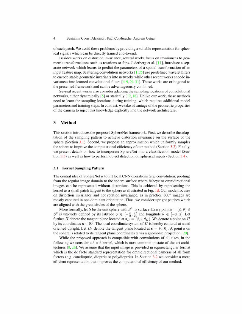
Fig. 3: Sampling Locations. This figure compares the sampling locations of SphereNet
(red) to the sampling locations of a regular CNN (blue) at the boundaries of the equirect-
angular image. Note how the SphereNet kernel automatically wraps at the left image
boundary (a) while correctly representing the discontinuities and distortions at the pole
(b). SphereNet thereby retains the original spherical image connectivity which is dis-
carded in a regular convolutional neural network that utilizes zero-padding along the
image boundaries.
The sampling grid locations of the convolutional kernels thus get distorted in the
same way as objects on a tangent plane of the sphere get distorted when projected from
different elevations to an equirectangular image representation. Fig. 2 demonstrates this
concept by visualizing the sampling pattern at two different elevations φ.
Besides encoding distortion invariance into the filters of convolutional neural net-
works, SphereNet additionally enables the network to wrap its sampling locations around
the sphere. As SphereNet uses custom sampling locations for sampling inputs or inter-
mediary feature maps, it is straightforward to allow a filter to sample data across the
image boundary. This eliminates any discontinuities which are present when process-
ing omnidirectional images with a regular convolutional neural network and improves
recognition of objects which are split at the sides of an equirectangular image represen-
tation or which are positioned very close to the poles, see Fig. 3.
By changing the sampling locations of the convolutional kernels while keeping their
size unchanged, our model additionally enables the transfer of CNN models between
different image representations. In our experimental evaluation, we demonstrate how an
object detector trained on perspective images can be successfully applied to the omnidi-
rectional case. Note that our method can be used for adapting almost any existing deep
learning architecture from perspective images to the omnidirectional setup. In general,
our SphereNet framework can be applied as long as the image can be mapped to the unit
sphere. This is true for many imaging models, ranging from perspective over fisheye4
to omnidirectional models. Thus, SphereNet can be seen as a generalization of regular
CNNs which encodes the camera geometry into the network architecture.
Implementation: As the sampling locations are fixed according to the geometry of
the spherical image representation, they can be precomputed for each kernel location at
4 While in some cases the single viewpoint assumption is violated, the deviations are often small
in practice and can be neglected at larger distances.

SphereNet: Learning Spherical Representations in Omnidirectional Images 7
every layer of the network. Further, their relative positioning is constant in each image
row. Therefore, it is sufficient to calculate and store the sampling locations once per
row and then translate them. We store the sampling locations in look-up tables. These
look-up tables are used in a customized convolution operation which is based on highly
optimized general matrix multiply (GEMM) functions [13]. As the sampling locations
are real-valued, interpolation of the input feature maps is required. In our experiments,
we compare nearest neighbor interpolation to bilinear interpolation. For an arbitrary
sampling location (px, py) in a feature map f , interpolation is defined as:
f(px, py) =H∑
n
W∑
m
f(m,n)g(px,m)g(py, n) (12)
with a bilinear interpolation kernel:
g(a, b) = max(0, 1− |a− b|) (13)
or a nearest neighbor kernel :
g(a, b) = δ(⌊a+ 0.5⌋ − b) (14)
where δ(·) is the Kronecker delta function.
3.2 Uniform Sphere Sampling
In order to improve the computational efficiency of our method, we investigate a more
efficient sampling of the spherical image. The equirectangular representation oversam-
ples the spherical image in the polar regions (see Fig. 4a), which results in near duplicate
image processing operations in this area. We can avoid unnecessary computation in the
polar regions by applying our method to a representation where data is stored uniformly
on the sphere, in contrast to considering the pixels of the equirectangular image.
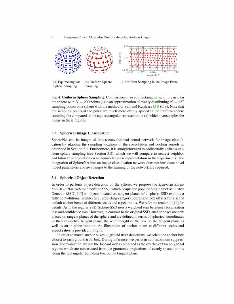
To sample points evenly from a sphere, we leverage the method of Saff and Kuijlaars
[24] as it is fast to compute and works with an arbitrary number of sampling points
N , including large values of N . More specifically, we obtain points along a spiral that
encircles the sphere in a way that the distance between adjacent points along the spiral is
approximately equal to the distance between successive coils of the spiral. As visualized
in Fig. 4 for an equirectangular image with Ne = 20× 10 = 200 sampling points, this
results in a sampling grid of N = 127 points with a similar sampling density to the
equirectangular representation at the equator, while significantly reducing the number
of sampling points at the poles.
To minimize the loss of information when sampling the equirectangular image we
use bilinear interpolation. Afterwards, the image is represented by an N × c matrix,
where c is the number of image channels. Unlike the equirectangular format, this rep-
resentation no longer encodes the spatial position of each data point. Thus, we save this
information in a separate matrix. This location matrix is used to compute the look-up ta-
bles for the kernel sampling locations as described in Section 3.1. Downsampling of the
image is implemented by recalculating a reduced set of sampling points. For applying
the kernels and downsampling the image nearest neighbor interpolation is used.
8 Benjamin Coors, Alexandru Paul Condurache, Andreas Geiger
(a) Equirectangular
Sphere Sampling
(b) Uniform Sphere
Sampling
.
−3.142 −1.571 0.000 1.571 3.142
longitude θ
−1.57
0.00
1.57
latitudeφ
(c) Uniform Sampling in the Image Plane
Fig. 4: Uniform Sphere Sampling. Comparison of an equirectangular sampling grid on
the sphere with N = 200 points (a) to an approximation of evenly distributing N = 127sampling points on a sphere with the method of Saff and Kuijlaars [24] (b, c). Note that
the sampling points at the poles are much more evenly spaced in the uniform sphere
sampling (b) compared to the equirectangular representation (a) which oversamples the
image in these regions.
3.3 Spherical Image Classification
SphereNet can be integrated into a convolutional neural network for image classifi-
cation by adapting the sampling locations of the convolution and pooling kernels as
described in Section 3.1. Furthermore, it is straightforward to additionally utilize a uni-
form sphere sampling (see Section 3.2), which we will compare to nearest neighbor
and bilinear interpolation on an equirectangular representation in the experiments. The
integration of SphereNet into an image classification network does not introduce novel
model parameters and no changes to the training of the network are required.
3.4 Spherical Object Detection
In order to perform object detection on the sphere, we propose the Spherical Single
Shot MultiBox Detector (Sphere-SSD), which adapts the popular Single Shot MultiBox
Detector (SSD) [17] to objects located on tangent planes of a sphere. SSD exploits a
fully convolutional architecture, predicting category scores and box offsets for a set of
default anchor boxes of different scales and aspect ratios. We refer the reader to [17] for
details. As in the regular SSD, Sphere-SSD uses a weighted sum between a localization
loss and confidence loss. However, in contrast to the original SSD, anchor boxes are now
placed on tangent planes of the sphere and are defined in terms of spherical coordinates
of their respective tangent plane, the width/height of the box on the tangent plane as
well as an in-plane rotation. An illustration of anchor boxes at different scales and
aspect ratios is provided in Fig. 5.
In order to match anchor boxes to ground truth detections, we select the anchor box
closest to each ground truth box. During inference, we perform non-maximum suppres-
sion. For evaluation, we use the Jaccard index computed as the overlap of two polygonal
regions which are constructed from the gnomonic projections of evenly spaced points
along the rectangular bounding box on the tangent plane.
SphereNet: Learning Spherical Representations in Omnidirectional Images 9
(a) Sphere
−3.142 −1.571 0.000 1.571 3.142
longitude θ
−1.57
0.00
1.57
latitudeφ
(b) Equirectangular
Fig. 5: Spherical Anchor Boxes are gnomonic projections of 2D bounding boxes of
various scales, aspect ratios and orientations on tangent planes of the sphere. The above
figure visualizes anchors of the same orientation at different scales and aspect ratios on
a 16× 8 feature map on a sphere (a) and an equirectangular grid (b).
4 Experimental Evaluation
While the main focus of this paper is on the detection task, we first validate our model
with respect to several existing state-of-the-art methods using a simple omnidirectional
MNIST classification task.
4.1 Classification: Omni-MNIST
For the classification task, we create an omnidirectional MNIST dataset (Omni-MNIST),
where MNIST digits are placed on tangent planes of the image sphere and an equirect-
angular image of the scene is rendered at a resolution of 60× 60 pixels.
We compare the performance of our method to several baselines. First, we trained a
regular convolutional network operating on the equirectangular images (EquirectCNN)
as well as one operating on a cube map representation of the input (CubeMapCNN).
We further improved the EquirectCNN model by combining it with a Spherical Trans-
former Network (SphereTN) which learns to undistort parts of the image by performing
a global rotation of the sphere. A more in-depth description of the Spherical Trans-
former Network is provided in the supplemental. Finally, we also trained the graph
convolutional network of Khasanova et al. [14] and the spherical convolutional model
of Cohen et al. [3]. For [3] we use the code published by the authors5. As [14] does not
provide code, we reimplemented their model based on the code of Defferrard et al. [6]6.
The network architecture for all models consist of two blocks of convolution and
max-pooling, followed by a fully-connected layer. We use 32 filters in the first and 64filters in the second layer and each layer is followed by a ReLU activation. The fully
connected layer has 10 output neurons and uses a softmax activation function. In the
CNN and SphereNet models, the convolutional filter kernels are of size 5 × 5 and are
applied with stride 1. Max pooling is performed with kernels of size 3× 3 and a stride
of 2. The Spherical Transformer Network uses an identical network architecture but
replaces the fully-connected output layer with a convolutional layer that outputs the
5 https://github.com/jonas-koehler/s2cnn6 https://github.com/mdeff/cnn graph
10 Benjamin Coors, Alexandru Paul Condurache, Andreas Geiger
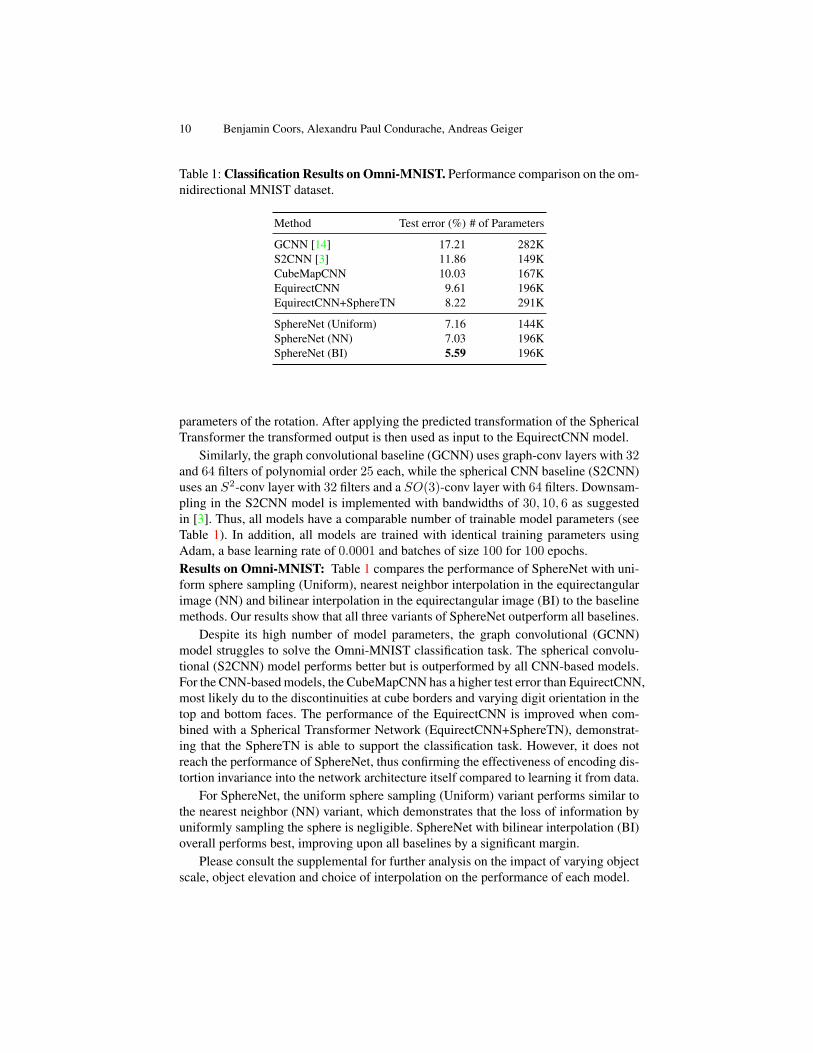
Table 1: Classification Results on Omni-MNIST. Performance comparison on the om-
nidirectional MNIST dataset.
Method Test error (%) # of Parameters
GCNN [14] 17.21 282K
S2CNN [3] 11.86 149K
CubeMapCNN 10.03 167K
EquirectCNN 9.61 196K
EquirectCNN+SphereTN 8.22 291K
SphereNet (Uniform) 7.16 144K
SphereNet (NN) 7.03 196K
SphereNet (BI) 5.59 196K
parameters of the rotation. After applying the predicted transformation of the Spherical
Transformer the transformed output is then used as input to the EquirectCNN model.
Similarly, the graph convolutional baseline (GCNN) uses graph-conv layers with 32and 64 filters of polynomial order 25 each, while the spherical CNN baseline (S2CNN)
uses an S2-conv layer with 32 filters and a SO(3)-conv layer with 64 filters. Downsam-
pling in the S2CNN model is implemented with bandwidths of 30, 10, 6 as suggested
in [3]. Thus, all models have a comparable number of trainable model parameters (see
Table 1). In addition, all models are trained with identical training parameters using
Adam, a base learning rate of 0.0001 and batches of size 100 for 100 epochs.
Results on Omni-MNIST: Table 1 compares the performance of SphereNet with uni-
form sphere sampling (Uniform), nearest neighbor interpolation in the equirectangular
image (NN) and bilinear interpolation in the equirectangular image (BI) to the baseline
methods. Our results show that all three variants of SphereNet outperform all baselines.
Despite its high number of model parameters, the graph convolutional (GCNN)
model struggles to solve the Omni-MNIST classification task. The spherical convolu-
tional (S2CNN) model performs better but is outperformed by all CNN-based models.
For the CNN-based models, the CubeMapCNN has a higher test error than EquirectCNN,
most likely du to the discontinuities at cube borders and varying digit orientation in the
top and bottom faces. The performance of the EquirectCNN is improved when com-
bined with a Spherical Transformer Network (EquirectCNN+SphereTN), demonstrat-
ing that the SphereTN is able to support the classification task. However, it does not
reach the performance of SphereNet, thus confirming the effectiveness of encoding dis-
tortion invariance into the network architecture itself compared to learning it from data.
For SphereNet, the uniform sphere sampling (Uniform) variant performs similar to
the nearest neighbor (NN) variant, which demonstrates that the loss of information by
uniformly sampling the sphere is negligible. SphereNet with bilinear interpolation (BI)
overall performs best, improving upon all baselines by a significant margin.
Please consult the supplemental for further analysis on the impact of varying object
scale, object elevation and choice of interpolation on the performance of each model.
SphereNet: Learning Spherical Representations in Omnidirectional Images 11
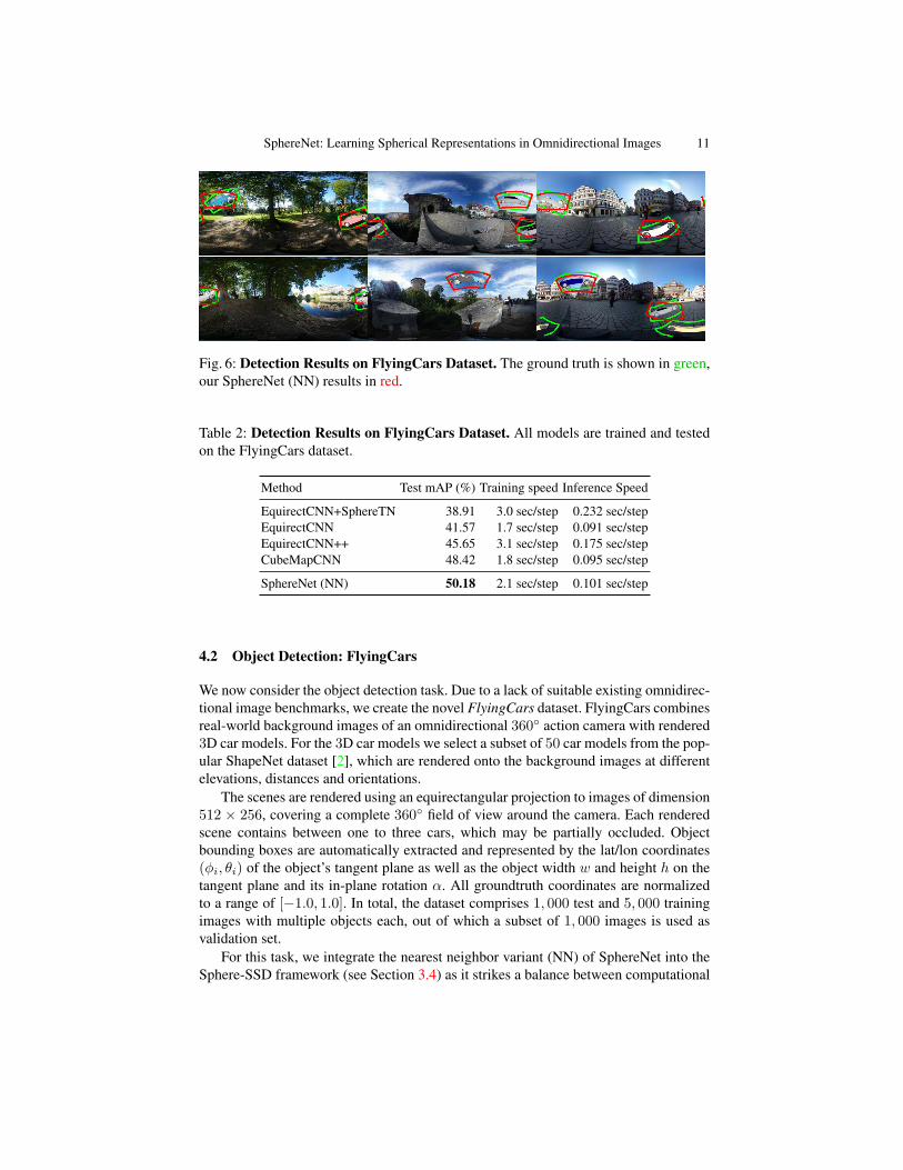
Fig. 6: Detection Results on FlyingCars Dataset. The ground truth is shown in green,
our SphereNet (NN) results in red.
Table 2: Detection Results on FlyingCars Dataset. All models are trained and tested
on the FlyingCars dataset.
Method Test mAP (%) Training speed Inference Speed
EquirectCNN+SphereTN 38.91 3.0 sec/step 0.232 sec/step
EquirectCNN 41.57 1.7 sec/step 0.091 sec/step
EquirectCNN++ 45.65 3.1 sec/step 0.175 sec/step
CubeMapCNN 48.42 1.8 sec/step 0.095 sec/step
SphereNet (NN) 50.18 2.1 sec/step 0.101 sec/step
4.2 Object Detection: FlyingCars
We now consider the object detection task. Due to a lack of suitable existing omnidirec-
tional image benchmarks, we create the novel FlyingCars dataset. FlyingCars combines
real-world background images of an omnidirectional 360◦ action camera with rendered
3D car models. For the 3D car models we select a subset of 50 car models from the pop-
ular ShapeNet dataset [2], which are rendered onto the background images at different
elevations, distances and orientations.
The scenes are rendered using an equirectangular projection to images of dimension
512 × 256, covering a complete 360◦ field of view around the camera. Each rendered
scene contains between one to three cars, which may be partially occluded. Object
bounding boxes are automatically extracted and represented by the lat/lon coordinates
(φi, θi) of the object’s tangent plane as well as the object width w and height h on the
tangent plane and its in-plane rotation α. All groundtruth coordinates are normalized
to a range of [−1.0, 1.0]. In total, the dataset comprises 1, 000 test and 5, 000 training
images with multiple objects each, out of which a subset of 1, 000 images is used as
validation set.
For this task, we integrate the nearest neighbor variant (NN) of SphereNet into the
Sphere-SSD framework (see Section 3.4) as it strikes a balance between computational
12 Benjamin Coors, Alexandru Paul Condurache, Andreas Geiger
efficiency and ease of integration into an object detection model. Because the graph
and spherical convolution baselines are not applicable to the object detection task, we
compare the performance of SphereNet to a CNN operating on the cube map (Cube-
MapCNN) and equirectangular representation (EquirectCNN). The latter is again tested
in combination with a Spherical Transformer Network (EquirectCNN+SphereTN).
Following [30] we evaluate a version of EquirectCNN where the size of the con-
volutional kernels is enlarged towards the poles to approximate the object distortion
in equirectangular images (EquirectCNN++). Like [30] we limit the maximum kernel
dimension to 7 × 7. However, unlike [30] we keep weight tying in place for image
rows with filters of the same dimension, thus reducing the number of model parame-
ters. We thereby enable regular training of the network without kernel-wise knowledge
distillation as in [30]. In addition, we utilize pre-trained weights when kernel dimen-
sions match with the kernels in a pre-trained network architecture so that not all model
parameters need to be trained from scratch.
As feature extractor all models use a VGG-16 network [26], which is initialized
with weights pre-trained on the ILSVRC-2012-CLS dataset [23]. We change the max-
pooling kernels to size 3 × 3 and use ReLU activations, L2 regularization with weight
4e−5 and batch normalization in all layers of the network. Additional convolutional box
prediction layers of depth 256, 128, 128, 128 are attached to layer conv5 3. Anchors of
scale 0.2 to 0.95 are generated for layer conv4 3, conv5 3 and the box prediction layers.
The aspect ratio for all anchor boxes is fixed to the aspect ratio of the side view of
the rendered cars (2 : 1). The full network is trained end-to-end in the Sphere-SSD
framework with the RMSProp optimizer, batches of size 5 and a learning rate of 0.004.
Results on FlyingCars: Table 2 presents the results for the object detection task on
the FlyingCars dataset after 50, 000 steps of training. Following common practice, we
use an intersection-over-union (IoU) threshold of 0.5 for evaluation. Again, our results
demonstrate that SphereNet outperforms the baseline methods. Qualitative results of
the SphereNet model are shown in Fig. 6.
Compared to the classification experiments, the Spherical Transformer Network
(SphereTN) demonstrates less competitive performance as no transformation is able to
account for undistorting all objects in the image at the same time. It is thus outperformed
by the EquirectCNN. The performance of the EquirectCNN model is improved when
the kernel size is enlarged towards the poles (EquirectCNN++), but all EquirectCNN
models perform worse than the CNN operating on a cube map representation (Cube-
MapCNN). The reason for the improved performance of the CubeMapCNN compared
to the classification task is most likely that discontinuities at the patch boundaries are
less often present in the FlyingCars dataset due to the smaller relative size of the objects.
Besides accuracy, another important property of an object detector is its training
and inference speed. Table 2 therefore additionally lists the training time per batch and
inference time per image on an NVIDIA Tesla K20. The numbers show similar run-
times for EquirectCNN and CubeMapCNN. SphereNet has a small runtime overhead
of factor 1.1 to 1.2, while the EquirectCNN++ and EquirectCNN+SphereTN models
have a larger runtime overhead of factor 1.8 for training and 1.9 to 2.5 for inference.

SphereNet: Learning Spherical Representations in Omnidirectional Images 13
Fig. 7: Detection Results on OmPaCa Dataset. The ground truth is shown in green,
our SphereNet (NN) results in red.
Table 3: Transfer Learning Results on OmPaCa Dataset. We transfer detection mod-
els trained on perspective images from the KITTI dataset [7] to an omnidirectional rep-
resentation and finetune the models on the OmPaCa dataset.
Method Test mAP (%)
CubeMapCNN 34.19
EquirectCNN 43.43
SphereNet (NN) 49.73
4.3 Transfer Learning: OmPaCa
Finally, we consider the transfer learning task, where a model trained on a perspective
dataset is transferred to handle omnidirectional imagery. For this task we record a new
real-world dataset of omnidirectional images of real cars with a handheld action cam-
era. The images are recorded at different heights and orientations. The omnidirectional
parked cars (OmPaCa) dataset consists of 1, 200 labeled images of size 512×256 with
more than 50 different car models in total. The dataset is split into 200 test and 1, 000training instances, out of which a subset of 200 is used for validation.
We use the same detection architecture and training parameters as in Section 4.2 but
now start from a perspective SSD model trained on the KITTI dataset [7], convert it to
our Sphere-SSD framework and fine-tune for 20, 000 iterations on the OmPaCa dataset.
For this experiment we only compare against the EquirectCNN and CubeMapCNN
baselines. Both the EquirectCNN+SphereTN as well as the EquirectCNN++ are not
well suited for the transfer learning task due to the introduction of new model param-
eters, which are not present in the perspective detection model and which would thus
require training from scratch.
Results on OmPaCa: Our results for the transfer learning task on the OmPaCa dataset
are shown in Table 3 and demonstrate that SphereNet outperforms both baselines. Un-
like in the object detection experiments on the FlyingCars dataset, the CubeMapCNN

14 Benjamin Coors, Alexandru Paul Condurache, Andreas Geiger
performs worse than the EquirectCNN by a large margin of nearly 10%, indicating
that the cube map representation is not well suited for the transfer of perspective mod-
els to omnidirectional images. On the other hand, SphereNet performs better than the
EquirectCNN by more than 5%, which confirms that the SphereNet approach is better
suited for transferring perspective models to the omnidirectional case.
A selection of qualitative results for the SphereNet model is visualized in Fig. 7. As
evidenced by our experiments, the SphereNet model is able to detect cars at different
elevations on the sphere including the polar regions where regular convolutional object
detectors fail due to the heavy distortions present in the input images. Several additional
qualitative comparisons between SphereNet and the EquirectCNN model for objects
located in the polar regions are provided in the supplementary material.
5 Conclusion and Future Work
We presented SphereNet, a framework for deep learning with 360◦ cameras. SphereNet
lifts 2D convolutional neural networks to the surface of the unit sphere. By applying 2D
convolution and pooling filters directly on the sphere’s surface, our model effectively
encodes distortion invariance into the filters of convolutional neural networks. Wrap-
ping the convolutional filters around the sphere further avoids discontinuities at the
borders or poles of the equirectangular projection. By updating the sampling locations
of the convolutional filters we allow for easily transferring perspective CNN models
to handle omnidirectional inputs. Our experiments show that the proposed method im-
proves upon a variety of strong baselines in both omnidirectional image classification
and object detection.
We expect that with the increasing availability and popularity of omnidirectional
sensors in both the consumer market (e.g., action cameras) as well as in industry (e.g.,
autonomous cars, virtual reality), the demand for specialized models for omnidirec-
tional images such as SphereNet will increase in the near future. We therefore plan to
exploit the flexibility of our framework by applying it to other related computer vision
tasks, including semantic (instance) segmentation, optical flow and scene flow estima-
tion, single image depth prediction and multi-view 3D reconstruction in the future.
References
1. Bruna, J., Mallat, S.: Invariant scattering convolution networks. IEEE Trans. on Pattern Anal-
ysis and Machine Intelligence (PAMI) 35(8), 1872–1886 (2013) 4
2. Chang, A.X., Funkhouser, T.A., Guibas, L.J., Hanrahan, P., Huang, Q., Li, Z., Savarese, S.,
Savva, M., Song, S., Su, H., Xiao, J., Yi, L., Yu, F.: Shapenet: An information-rich 3d model
repository. arXiv.org 1512.03012 (2015) 11
3. Cohen, T.S., Geiger, M., Kohler, J., Welling, M.: Spherical CNNs. In: International Confer-
ence on Learning Representations (2018) 3, 9, 10
4. Cohen, T.S., Welling, M.: Group equivariant convolutional networks. In: Proc. of the Inter-
national Conf. on Machine learning (ICML) (2016) 2, 4
5. Dai, J., Qi, H., Xiong, Y., Li, Y., Zhang, G., Hu, H., Wei, Y.: Deformable convolutional
networks. Proc. of the IEEE International Conf. on Computer Vision (ICCV) 1703.06211
(2017) 4
SphereNet: Learning Spherical Representations in Omnidirectional Images 15
6. Defferrard, M., Bresson, X., Vandergheynst, P.: Convolutional neural networks on graphs
with fast localized spectral filtering. In: Advances in Neural Information Processing Systems
(NIPS) (2016) 9
7. Geiger, A., Lenz, P., Urtasun, R.: Are we ready for autonomous driving? The KITTI vision
benchmark suite. In: Proc. IEEE Conf. on Computer Vision and Pattern Recognition (CVPR)
(2012) 13
8. He, K., Zhang, X., Ren, S., Sun, J.: Deep residual learning for image recognition. In: Proc.
IEEE Conf. on Computer Vision and Pattern Recognition (CVPR) (2016) 4
9. Henriques, J.F., Vedaldi, A.: Warped convolutions: Efficient invariance to spatial transforma-
tions. In: Proc. of the International Conf. on Machine learning (ICML) (2017) 4
10. Hu, H.N., Lin, Y.C., Liu, M.Y., Cheng, H.T., Chang, Y.J., Sun, M.: Deep 360 pilot: Learning
a deep agent for piloting through 360◦ sports video. In: Proc. IEEE Conf. on Computer
Vision and Pattern Recognition (CVPR) (2017) 1
11. Jaderberg, M., Simonyan, K., Zisserman, A., Kavukcuoglu, K.: Spatial transformer net-
works. In: Advances in Neural Information Processing Systems (NIPS) (2015) 4
12. Jeon, Y., Kim, J.: Active convolution: Learning the shape of convolution for image classifi-
cation. In: Proc. IEEE Conf. on Computer Vision and Pattern Recognition (CVPR) (2017)
4
13. Jia, Y.: Learning Semantic Image Representations at a Large Scale. Ph.D. thesis, EECS De-
partment, University of California, Berkeley (May 2014), http://www2.eecs.berkeley.edu/
Pubs/TechRpts/2014/EECS-2014-93.html 7
14. Khasanova, R., Frossard, P.: Graph-based classification of omnidirectional images. In: Proc.
of the IEEE International Conf. on Computer Vision (ICCV) Workshops (2017) 3, 9, 10
15. Khasanova, R., Frossard, P.: Graph-based isometry invariant representation learning. In:
Proc. of the International Conf. on Machine learning (ICML) (2017) 3
16. Lai, W., Huang, Y., Joshi, N., Buehler, C., Yang, M., Kang, S.B.: Semantic-driven generation
of hyperlapse from 360 degree video (2017) 1
17. Liu, W., Anguelov, D., Erhan, D., Szegedy, C., Reed, S.E., Fu, C., Berg, A.C.: SSD: single
shot multibox detector. In: Proc. of the European Conf. on Computer Vision (ECCV) (2016)
8
18. Ma, J., Wang, W., Wang, L.: Irregular convolutional neural networks (2017) 4
19. Monroy, R., Lutz, S., Chalasani, T., Smolic, A.: Salnet360: Saliency maps for omni-
directional images with cnn. In: ICME (2017) 3
20. Pearson, F.: Map Projections: Theory and Applications. Taylor & Francis (1990) 4, 5
21. Ran, L., Zhang, Y., Zhang, Q., Yang, T.: Convolutional neural network-based robot naviga-
tion using uncalibrated spherical images. Sensors 17(6) (2017) 1
22. Ruder, M., Dosovitskiy, A., Brox, T.: Artistic style transfer for videos and spherical images.
arXiv.org abs/1708.04538 (2017) 3
23. Russakovsky, O., Deng, J., Su, H., Krause, J., Satheesh, S., Ma, S., Huang, Z., Karpathy, A.,
Khosla, A., Bernstein, M., Berg, A.C., Fei-Fei, L.: Imagenet large scale visual recognition
challenge. International Journal of Computer Vision (IJCV) (2015) 12
24. Saff, E.B., Kuijlaars, A.B.J.: Distributing many points on a sphere. The Mathematical Intel-
ligencer 19(1), 5–11 (1997) 7, 8
25. Sifre, L., Mallat, S.: Rotation, scaling and deformation invariant scattering for texture dis-
crimination. In: Proc. IEEE Conf. on Computer Vision and Pattern Recognition (CVPR)
(2013) 4
26. Simonyan, K., Zisserman, A.: Very deep convolutional networks for large-scale image recog-
nition. In: Proc. of the International Conf. on Learning Representations (ICLR) (2015) 4, 12
27. Su, Y.C., Grauman, K.: Making 360deg video watchable in 2d: Learning videography for
click free viewing. In: Proc. IEEE Conf. on Computer Vision and Pattern Recognition
(CVPR) (2017) 1

16 Benjamin Coors, Alexandru Paul Condurache, Andreas Geiger
28. Su, Y.C., Jayaraman, D., Grauman, K.: Pano2vid: Automatic cinematography for watching
360 degree videos. In: Proc. of the Asian Conf. on Computer Vision (ACCV) (2016) 1
29. Worrall, D.E., Garbin, S.J., Turmukhambetov, D., Brostow, G.J.: Harmonic networks: Deep
translation and rotation equivariance. In: Proc. IEEE Conf. on Computer Vision and Pattern
Recognition (CVPR) (2017) 2, 4
30. Yu-Chuan Su, K.G.: Flat2sphere: Learning spherical convolution for fast features from 360◦
imagery. In: Advances in Neural Information Processing Systems (NIPS) (2017) 3, 12
31. Zhou, Y., Ye, Q., Qiu, Q., Jiao, J.: Oriented response networks. In: Proc. IEEE Conf. on
Computer Vision and Pattern Recognition (CVPR) (2017) 4
Recommended