Acoustic-based techniques for autonomousunderwater vehicle localizationY Petillot1*, F Maurelli1, N Valeyrie1, A Mallios2, P Ridao2, J Aulinas2, and J Salvi2
1Ocean Systems Laboratory, Herriot–Watt University, Edinburgh, UK2Office 016 - PIV, Escola Politecnica Superior, Campus de Montilivi, Girona, Spain
The manuscript was received on 1 December 2009 and was accepted after revision for publication on 9 June 2010.
DOI: 10.1243/14750902JEME197
Abstract: This paper presents two acoustic-based techniques to solve the localization problemfor an autonomous underwater vehicle (AUV). After a brief description of the Bayesian filteringframework, the paper analyses two of the most common underwater scenarios. Each scenariocorresponds to one of the two localization techniques. The scenarios are as follows: map-basedlocalization, when the environment is sufficiently distinctive; transponder-based localization fornavigation in large and not distinctive environments. An environment is said to be distinctivewhen there are possible reference points. For example, a completely flat featureless sea floor isnot considered as distinctive. The proposed techniques were validated in simulation. The map-based localization technique was also validated in trials with the autonomous underwatervehicles Ictineu and Nessie IV. The trials with Ictineu took place in an abandoned marina withIctineu travelling along a trajectory that was more than 600 m long. The trials with Nessie IV tookplace in a rectangular pool and during an AUV competition.
Keywords: localization problem, autonomous underwater vehicle, acoustic-based techniques
1 INTRODUCTION
Over the past few years, underwater technology has
significantly grown and remotely operated vehicles
(ROVs) are nowadays safely and routinely used in the
offshore industry. ROVs are constantly controlled by a
human operator. Other vehicles called autonomous
underwater vehicles (AUVs) have received much
attention from the underwater robotic community
because of their ability to carry out missions without
close human intervention and supervision. There are
many open research areas related to AUVs such as safe
and reliable autonomous navigation. An autonomous
vehicle indeed needs to demonstrate high autonomy
in order to keep track of its position and orientation
and to build a map of this environment while suc-
cessfully completing autonomous tasks. Many ap-
proaches have been developed for land and aerial
vehicles [1–3]. However, the constraints and peculia-
rities of the underwater environment prevent the
direct application of techniques developed for land or
aerial vehicles in the underwater domain. A careful
study of each technique with regard to the constraints
of the underwater domain is required.
The primary navigation system used in land, aerial,
and underwater applications is the inertial measure-
ment unit (IMU), which provides an estimation of the
acceleration of the vehicle. In addition to being
expensive, this system suffers from drift errors, which,
doubly integrated over time, result in the need for
some external system to correct the localization
errors. In land and aerial robotics, this can be achieved
by incorporating Global Positioning System (GPS)
measurements. The GPS signal is not available in an
underwater environment and other techniques to
correct the drift errors of the IMU are needed. The
IMU is also not able to give an absolute localization
but only an estimation of the inertial movement.
There are, then, many cases in which the IMU alone
fails to provide accurate localization. This happens
when the starting position is unknown or in the
*Corresponding author: Ocean Systems Laboratory, Herriot–Watt
University, Earl Mountbatten Building, Riccarton, Edinburgh
EH14 4AS, UK.
email: [email protected]
SPECIAL ISSUE PAPER 293
JEME197 Proc. IMechE Vol. 224 Part M: J. Engineering for the Maritime Environment

classical kidnapped robot problem [4] where the robot
starts from an unknown position in a known environ-
ment and needs to determine its position. Providing
only relative values, the IMU is also not able to recover
after an incorrect localization. Similar considerations
are valid for the Doppler velocity log (DVL), which
provides an estimation of the velocity vector using
acoustic measurements.
The absence of a GPS signal and the difficult sensing
conditions make underwater localization a complex
problem. The lack of visibility and scattering make the
use of cameras difficult, if not impossible, at long
ranges. Precise laser range finders, widely exploited for
land robots, cannot be used efficiently in the water. As
a consequence, acoustic techniques are the most
widely used and have specific problems such as high
noise, poor resolution, and slow frame rate.
This paper investigates solutions to two problems.
1. AUV localization. In this case, the environment is
known a priori and a local map of the environment
is captured by an imaging sonar. The algorithm
uses the local sonar map to localize itself in the
known global map. This is a typical problem for
deep-water inspection of structures or port and
harbour surveillance where the environment is well
known but the vehicle’s position is not accurate by
the time that it has reached the area of interest for
the mission.
2. Beacon-based simultaneous localization and map-
ping (SLAM). In this case, the environment is un-
known and feature poor. Classical feature-based
mapping and localization techniques cannot be
used. In the present approach, the environment is
composed of acoustic transponders whose posi-
tions are a priori unknown. It has been assumed
that the transponders broadcast only range infor-
mation which corresponds to the current state of
the art in readily available transponders technol-
ogy. The algorithm presented here estimates jointly
the position of the vehicle and the position of the
beacons. This can be seen as a self-calibrating long-
baseline (LBL) system.
It is, then, possible to imagine a system built on
the two solutions presented here which solves the
full localization problem; in open water, the vehicle
deploys beacons as it moves and uses the network
generated to localize until it reaches a structure that
requires closer inspection for which some a priori
information is known (a local map, for instance).
The particle filter localization algorithm is used for
this task.
1.1 Related work
Several techniques have been proposed for AUV loca-
lization. Caiti et al. [5] developed an acoustic localiza-
tion technique using freely floating acoustic buoys
equipped with GPS connection. This system requires
the buoys to emit a ping at regular time intervals with
coded information of its GPS position. The vehicle can
locate itself using time-of-flight measurements of
acoustic pings from each buoy. The limitations of this
approach are the necessity to deploy a sufficient num-
ber of floating buoys in the mission area, the need to
collect them after the end of the mission, and a non-
efficient communication scheme, as the buoys peri-
odically send acoustic messages. Limitations for deep-
water missions are also evident. Erol et al. [6] pro-
posed to use GPS-aided localization. The problem in
this approach is that the GPS signal does not propa-
gate in the water. The AUV is therefore forced to
acquire the signal at the surface. This approach is not
very reliable, since the vehicle has no access to a GPS
signal during the submerged period and has to
estimate its state with other sensors. To handle this
problem, the vehicle dives to a fixed depth and follows
a predefined trajectory, which is not suitable for
navigation in complex environments.
Other acoustic-based localization techniques in-
clude the LBL, short-baseline (SBL), and ultra-short-
basline (USBL) systems. In these cases, the vehicle’s
position is determined on the basis of the acoustic
returns detected by a set of receivers. For LBL sys-
tems, a set of acoustic transponders is first deployed
in the area of operation. The vehicle is then able to
locate itself with respect to the transponders (or, in
the opposite way, the transponders are able to track
the vehicle), as explained in reference [7]. For SBL
and USBL systems, Storkensen et al. [8] proposed to
use a support ship equipped with a high-frequency
directional emitter able to determine the AUV’s
position accurately with respect to the mother ship.
This approach requires, however, the support of a
ship. Furthermore, it cannot be used in many situa-
tions as it requires the ship and the vehicle to be
close to each other. This approach is therefore not
suitable for navigation around deep offshore struc-
tures. In terms of the computational framework,
particle filter techniques have been used for the
localization of underwater vehicles although not as
widely as for land and aerial vehicles. Karlsson et al.
[9] proposed a particle filter approach for AUV
navigation but the focus was more on the mapping
part than on the localization. Silver et al. [10] pre-
sented a particle filter merged with scan-matching
techniques. Recent work by Ortiz et al. [11] addressed
294 Y Petillot, F Maurelli, N Valeyrie, A Mallios, P Ridao, J Aulinas, and J Salvi
Proc. IMechE Vol. 224 Part M: J. Engineering for the Maritime Environment JEME197

the use of particle filters for tracking undersea narrow
telecommunication cables.
Regarding the SLAM problem, the earliest method
put forward uses an extended Kalman filter (EKF) to
estimate jointly the state of the AUV and the position
of the transponders [12]. This approach has been
used with success in various cases [13–15], but the
filter suffers from linearization of non-linear models
which can quickly lead to divergence as the covar-
iance estimates become unreliable. In addition, the
algorithmic complexity of the EKF algorithm grows
quadratically with the number of beacons (in the two-
dimensional (2D) case). For example, the prediction
step of the EKF not only affects the state of the AUV
but also involves the computation of the Jacobian of
the motion model which also takes into account the
transponders. Several methods have been put for-
ward to reduce the complexity of the EKF algorithm,
such as the linear state augmentation principle or the
partitioned update approach, both presented in
reference [16]. These methods have a linear complex-
ity with the number of beacons. Other solutions to the
SLAM problem are the extended information filter
[17], the unscented Kalman filter (UKF) [18], and the
FastSLAM algorithms [19].
1.2 Contribution
The present approach to the localization problem uses
the ability of the vehicle to sense the environment and
requires a general, but not too precise, a priori map of
the environment. Most algorithms proposed to date
(in air or an land) perform very well in small envi-
ronments but do not always scale well to large en-
vironments and long trajectories. The present ap-
proach extends this technique to the underwater
domain and demonstrates the robustness of a map-
based localization system in a real large-scale scenario.
Moreover, most of the approaches for localization
assume a perfect knowledge of the environment. This
assumption is unrealistic because the ground truth is
not available in many situations. Here, however, the
map generated [20] with a SLAM approach is used.
This map does integrate errors and the demonstration
that it can still be used validates the use of SLAM-
generated maps for other applications. For instance,
once the robot has built a coherent map on an
unknown environment, it is indeed desirable to use
the generated map for further activities in the same
portion of environment. The computational complex-
ity of localization decreases and it is easier for the
vehicle to perform other tasks in the area.
While the first approach is very useful to navigate
around underwater structures, the environment sur-
rounding the robot might not be sufficiently distinc-
tive to allow reliable localization (e.g. large areas with
a flat featureless seabed). Acoustic transponders
deployed in the area of interest help to localize the
vehicle. The position of the transponders is usually
unknown, in which case the vehicle has to localize
itself and the transponders simultaneously. A range-
only SLAM algorithm inspired by reference [21] is
proposed; this is based on a particle-filtering imple-
mentation of the SLAM problem and is coupled with a
mixture-of-Gaussians representation of the posterior
distribution of the beacon’s position. This is demon-
strated in the simulation and shows the potential of
the technique as a self-calibrating LBL system.
The paper is divided into four parts: the first part
presents the Bayesian filtering techniques for robot
localization. The next two parts address the two com-
mon scenarios in underwater localization: in closed
and open environments, with the use of particle filter
and Gaussian sum filter techniques. The fourth part
presents the experimental results, both in the simula-
tion and in real conditions. Finally, conclusions and
future work are detailed.
2 THE BAYESIAN FILTERING FRAMEWORK
2.1 Optimal Bayesian filtering
The state of the AUV at time t is a random vector
denoted by Xt that usually includes the position and
the speed of the AUV. The evolution of the AUV’s state
is provided by the motion model. Usually, the motion
model assumes that (Xk) is a Markov process entirely
defined by the transition kernel p(xk|xk 2 1) and the
distribution of the initial state X0. The transition
kernel is related to the measurements provided by the
IMU or the DVL that predict the future state of the
AUV, given its past state. The state Xt is not directly
observed but is known through measurements reg-
ularly gathered by the AUV. The measurements are,
for example, the scan of a rotating sonar or range of
measurements with respect to acoustic transponders.
The measurement at time t is a random vector
denoted by Yt that only depends on Xt. The measure-
ment model provides the conditional density p(yt|xt)
that statistically links the observation Yt to the state
Xt. These assumptions are those of a hidden Markov
model.
The objective in Bayesian filtering is to calculate the
conditional density p(xt|y0:t) so that an estimate of the
Acoustic-based techniques for AUV localization 295
JEME197 Proc. IMechE Vol. 224 Part M: J. Engineering for the Maritime Environment

state Xt can be obtained through the conditional
expectation
E X t jY 0:t½ �~ð
xtp xt jy0:tð Þdxt ð1Þ
This conditional expectation is the estimate of Xt,given Y0:t, which minimizes the mean square error,namely
E X t{E X t jY 0:t½ �j j2h i
¡E X t{y Y 0:tð Þj j2h i
ð2Þ
for any other estimate y(Y0:t) of Xt, given the obser-vations Y0:t. The conditional density p(xt|y0:t) may berecursively calculated from p(xt 2 1|y0:t 2 1) through theexact prediction and correction steps
p xt jy0:t{1ð Þ~ð
p xt{1jy0:t{1ð Þ p xt jxt{1ð Þ|fflfflfflfflfflfflffl{zfflfflfflfflfflfflffl}transition kernel
dxt{1 ð3Þ
and
p xt jy0:tð Þ~ctp xt jy0:t{1ð Þ p yt jxtð Þ|fflfflfflffl{zfflfflfflffl}measurement model
ð4Þ
The normalization constant ct is unknown and givenby
1
ct~
ðp xt jy0:tð Þdxt
~
ðp xt jy0:t{1ð Þp yt jxtð Þdxt ð5Þ
Assuming that the motion and the measurement
models are both linear and Gaussian, the distribution
of Xt|Y0:t is also Gaussian. The mean and the co-
variance matrix of Xt|Y0:t may then be calculated using
the recurrence relations of the Kalman filter [22, 23].
The calculation of the conditional expectation
E X t jY 0:t½ � is exact so that the Kalman filter is optimal;
i.e. it provides the estimate of Xt, given Y0:t, which
minimizes the mean square error mentioned pre-
viously.
The motion and the measurement models of an
AUV are seldom both linear and Gaussian. Conse-
quently, approximate and thereby suboptimal solu-
tions to the non-linear non-Gaussian Bayesian filtering
problem have to be provided. Various approximation
schemes have been put forward, among which are the
Monte Carlo and the sum of Gaussian approximations.
The former approximation is at the core of any particle
filter and the latter is known as the Gaussian sum filter.
2.2 Particle filters
Any particle filter relies on a Monte Carlo approxima-
tion of the conditional density p(xt|y0:t) using a finite
set of N points jit in the state space called particles.
The approximation is of the form
p xt jy0:tð Þ&XN
i~1
witdji
txtð Þ
where
XN
i~1
wit~1
ð6Þ
and where djit
denotes the usual Dirac function,
namely
djit
xð Þ~ 1 if x~jit
0 otherwise
(ð7Þ
Equation (6) may be interpreted in the following way:the denser the particles in a region of the state spaceand the higher their weights, the higher is the pro-bability that the state lies in this region. Assuming thatthe way in which samples can be obtained fromp(xt|y0:t) is known, the Monte Carlo approximationbecomes
p xt jy0:tð Þ&XN
i~1
1
Ndji
txtð Þ
with
jit*p xt jy0:tð Þ
ð8Þ
where , means ‘follows the distribution of’. Theprevious assumption is unrealistic, since it impliesthat the Bayesian filtering problem is solved. Any par-ticle filter relies on the importance sampling principlewhich provides a mechanism to build a Monte Carloapproximation of p(xt|y0:t).
Suppose that it is required to sample from a dis-
tribution whose density f is of the form
f xð Þ~cr xð Þg xð Þ
where
g 5 density of a distribution from which it is easy to
sample and which is called the proposal distribution
r 5 weighting function which is easy to evaluate
c 5R
f(x) dx is an unknown normalization constant
296 Y Petillot, F Maurelli, N Valeyrie, A Mallios, P Ridao, J Aulinas, and J Salvi
Proc. IMechE Vol. 224 Part M: J. Engineering for the Maritime Environment JEME197

The importance sampling principle provides the ap-
proximation for f as
f xð Þ&XN
i~1
widjixð Þ
with
jit*g xð Þ
ð9Þ
where the weights wi~f jið Þ.PN
j~1 f jj
� �are not equal
to 1/N, since they account for the particles being
generated using a distribution other than f.
The first particle filter ever proposed was the
bootstrap filter introduced by Gordon et al. [24] but
the most commonly used particle filter is the sampling
with importance resampling (SIR) filter. Other kinds of
particle filter such as the auxiliary particle filter or the
kernel filter have been introduced in order to improve
the performance of the SIR algorithm. The interested
reader can find an overview of the existing sequential
Monte Carlo methods for Bayesian filtering in refer-
ences [25] and [26].
The SIR filter intends to reproduce the optimal pre-
diction and correction steps of the optimal Bayesian
filter. The three steps of iteration t > 1 of the SIR algo-
rithm are as follows.
Step 1: selection: Generate tit* w1
t{1, . . . ,wNt{1
� �.
Step 2: propagation: Generate jit*p xt jj
tit
t{1
� �.
Step 3: correction: Set wit!p yt jji
t
� �.
In the SIR particle filter, the propagation step of
iteration t uses the transition kernel to simulate the
new set of particles j1t , . . . , jN
t
� �, as in the bootstrap
filter. However, only the most likely particles at time
t 2 1 are selected to generate the particles at time t.
The selection is made according to the weights, since
the higher a weight the more adequate are the obser-
vation of the corresponding particle. This selection
step makes the SIR particle filter more efficient than
the bootstrap filter.
2.3 Gaussian sum filter
Particle filters rely on a Monte Carlo approximation of
the distribution of Xt|Y0:t. They require a large number
of particles so that the approximation is sufficiently
accurate and thereby have a high computational cost.
A long time before the emergence of particle filters, an
approximation scheme based on a mixture of Gaussian
distributions was suggested by Alspach and Sorenson
[27]. This Gaussian sum approximation was shown to
perform better than the EKF while being compatible
with the computational capabilities of that time. The
conditional density p(xt|y0:t) is approximated by
p xt jy0:tð Þ&XN
i~1
aitC xt ; mi
t , Pit
� �
with
XN
i~1
ait~1
ð10Þ
where x ¨ C(x; m, P) denotes the probability densityfunction (PDF) of a Gaussian multi-variate distributionof mean m and covariance matrix P. The individual
means mit and individual covariance matrices and Pi
t
are updated according to the recurrence relations of
the EKF. The interested reader can find a complete
description of the Gaussian sum filter in reference [27].
2.4 Bayesian approach to the SLAM problem
The Bayesian filtering framework is suitable for esti-
mating the state Xt of an AUV. The SLAM problem
also requires the estimation of the state Xt together
with the estimation of the map of the environment. In
the SLAM problem considered in this paper, the envi-
ronment is composed of acoustic transponders
whose positions are to be found. The position of each
transponder is denoted by Bi and B denotes the set of
all the transponders.
The Bayesian approach to the SLAM problem re-
quires the calculation of the conditional density p(xt,
b|y0:t) so that an estimate of (Xt, B) can be obtained
through the conditional expectation
E X t , BjY 0:t½ �~ð
xt , bð Þp xt , bjy0:tð Þd xt , bð Þ ð11Þ
3 PARTICLE FILTER FOR LOCALIZATION IN ADISTINCTIVE ENVIRONMENT
The first scenario is when the vehicle can sense a
sufficiently distinctive environment. By distinctive is
meant that the sensor’s measures vary significantly
with position. A typical example is the navigation in
man-made environments, such as marinas, or navi-
gation close to underwater structures, both natural
Acoustic-based techniques for AUV localization 297
JEME197 Proc. IMechE Vol. 224 Part M: J. Engineering for the Maritime Environment

and artificial, such as an off-shore underwater oil
infrastructure.
The chosen approach uses particle filter techniques
for a variety of reasons. First, it can handle the estima-
tion of non-Gaussian and non-linear processes. This
is very important because non-linearities are very
frequent in AUVs, both in the motion model speci-
fication and in the observation process. Additionally,
the noise cannot be modelled as Gaussian in many
situations. Another advantage of using particle filters
is that it does not require any assumption on the
initial position and orientation of the vehicle. How-
ever, the standard approach presents two main
problems. The first is the large number of particles
required in order to explore the state space, resulting
in an increase in the computational power needed.
The other major issue in particle filter approaches is
the sample impoverishment problem, i.e. the loss of
diversity for the particles to represent the solution
space adequately [28]. In the present approach, both
these problems are addressed, as shown next.
3.1 Particle resampling
The standard SIR algorithm for particle resampling
lets the particles with high weights reproduce, while
the particle with low weights are more unlikely to
survive. However, the resulting PDF at time t depends
only on the PDF at time t 2 1. In time, this means that
only a small part of the state space is represented by
the particles and the system cannot recover from an
incorrect estimation of the vehicle’s position (owing to
sensor noise, for instance). In the present system, at
each step, a portion of the particles is instantiated
randomly in the state space. Thus, the resampling
algorithm is built with two modules. The first is a
standard SIR module, returning N 2 k particles. The
second module returns k particles, created randomly.
The combination of these two modules constitutes the
resampling step in the proposed system. The algo-
rithm is then able to recover in the case of a wrong
convergence, as shown in section 3.4. The benefits
from the computational point of view are also rele-
vant, since there is no need to instantiate a large
number of particles. Even if in the initial step there are
no particles near the real position of the vehicle, the
proposed solution is still able to find the correct
position, after some time, because of the partial
random resampling.
3.2 Sensor model and the likelihood calculation
The sensor used here is a forward-looking sonar
profiler which returns range profiles (Fig. 1). The
general idea to compute the likelihood is to compare
two arrays of distances. The first is the array generated
by the real sonar system, while the second is simulated
on the basis of the possible position of the vehicle
(given by the particle) and knowledge of the environ-
ment (a priori map). For the simulated set-up, a ray-
tracing algorithm was used to compute the intersec-
tion between the sonar beams and the environment.
In order to determine the array of distances for each
particle, an alternative solution to ray tracing has been
used. As the map given by Ribas et al. [20] is a set of
lines, a geometrical approach based on line intersec-
tion is much faster than and as accurate as ray tracing.
For the real tests, sonar data processing is required in
order to obtain the array of distances. The imaging
sonar returns for each beam an intensity array. To
transform this array to a distance value, a threshold is
applied in order to separate the acoustic imprint left
Fig. 1 Illustration of the calculation of the likelihood for the particle filter
298 Y Petillot, F Maurelli, N Valeyrie, A Mallios, P Ridao, J Aulinas, and J Salvi
Proc. IMechE Vol. 224 Part M: J. Engineering for the Maritime Environment JEME197

by an object in the image from the noisy background
data. Once the two arrays of distances have been
computed, the next problem is the likelihood calcula-
tion. The likelihood value should reflect the similarity
of the two arrays. To provide better understanding of
the proposed approach, the case of arrays composed
by a single element each (r and s) will now be
described. In this case, the likelihood is given by the
equation
L xð Þ~ 1ffiffiffiffiffiffi2pp exp {
1
2x2
� ð12Þ
where x 5 r 2 s, r represents the real value of distancegiven by the vehicle, and s represents the simulatedvalue given by the particles. In the case of arrays withmore than one value, the same procedure can beapplied to all indices of the array, producing a like-lihood array. In order to calculate a single likelihoodvalue, a mean-value solution was chosen. The like-lihood function calculated in this way is therefore amixture of Gaussians. A pure Gaussian likelihood wasalso tested, multiplying the likelihoods of the singleindices, like a joint probability of independent vari-ables. Both methods proved to be valid and reliable.However, the product method is more selective butalso more sensitive to noise, as a few bad-index like-lihoods have a great impact on the overall likelihood ofthe particle. On the other hand, the average methodseems to preserve better the diversity of the particlesin the solution state. Thus, it is to be preferred whenfew particles are used, while the product method is tobe preferred when there are many particles in thesame area, to discriminate better between them.
3.3 Motion model
For the simulated set-up, the motion model is simply
the difference between the ground truth positions at
time t and at time t 2 1, disturbed with some process
noise. The particle state is thus updated considering
that value, plus a different noise for each particle, in
order to explore more effectively the solution space
(Fig. 2). For the real set-up, the motion estimation is
given by the sensors. The Ictineu vehicle is equipped
with a SonTek Argonaut DVL unit which provides
bottom tracking and water velocity measurements at a
frequency of 1.5 Hz. Additionally, an MTi sensor, a
low-cost motion reference unit (MRU), provides atti-
tude data at a 0.1 Hz rate. These values are integrated
in an EKF. A six-degrees-of-freedom constant-velocity
kinematic model is used to predict the state of the
vehicle. Since AUVs are commonly operated describ-
ing rectilinear transects at a constant speed during
survey missions, such a model, although simple,
represents a realistic way to describe the motion.
3.4 Results
3.4.1 Results on simulated data
The first step in the validation of the proposed system
is by simulation. The present system can model a
vehicle with six degrees of freedom. In this particular
set-up it has been assumed that the pitch and roll of
the vehicle are neglected. Additionally, at this point,
the sensor’s orientation in relation to the vehicle is
fixed. A simulated gyroscope is used to have a noisy
estimation of the orientation of the vehicle’s heading
(yaw). A simulated depth sensor provides a noisy
estimation of the vehicle’s depth. Finally, a simulated
sonar is modelled to acquire range profiles. It is
assumed that an a priori map of the vehicle’s sur-
roundings is known. No assumptions are made on the
initial position of the vehicle within the map. The
particle state is represented by six variables (three for
the orientation and three for the position of the
vehicle), plus an additional variable representing the
weight of the particle.
A synthetic environment was created to validate the
approach. Different types of scenario were considered
in order to analyse the algorithm performances. The
system has proved to be valid for both structured and
unstructured scenarios. In more than 95 per cent of
cases, the algorithm converges to the real trajectory
before the end of the experiment. Two methods have
been explored in order to infer the trajectory, given
the particles’ state. The first method considers the
mean of the Monte Carlo approximation (i.e. the
weighted sum of the particles), and the second
method considers the best particle as an estimate of
the state of the AUV (a crude estimate of the mode of
the distribution). In the simulated set-up, the best
particle trajectory always gives better results, mini-
mizing both the time needed for convergence and the
overall error.
3.4.2 Results on real data
The localization system was tested on the same data
set used in reference [20] to perform underwater
SLAM. The data were gathered during an extensive
survey of an abandoned marina on the Costa Brava
(Spain). The Ictineu AUV gathered a data set along a
600 m trajectory which included a small loop around
the principal water tank and a 200 m straight path
through an outgoing canal. The data set included
Acoustic-based techniques for AUV localization 299
JEME197 Proc. IMechE Vol. 224 Part M: J. Engineering for the Maritime Environment
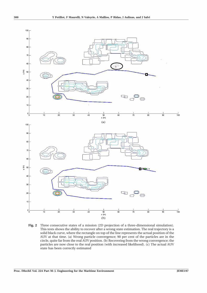
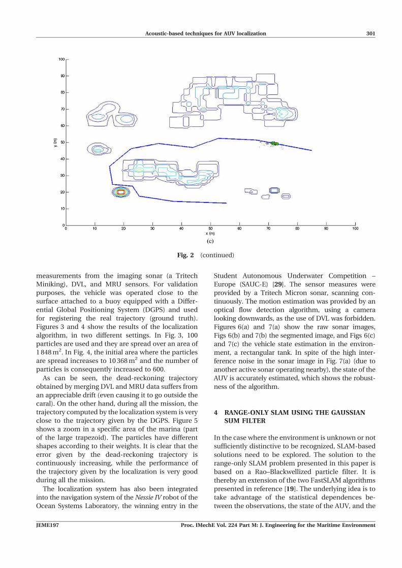
Fig. 2 Three consecutive states of a mission (2D projection of a three-dimensional simulation).This tests shows the ability to recover after a wrong state estimation. The real trajectory is asolid black curve, where the rectangle on top of the line represents the actual position of theAUV at that time. (a) Wrong particle convergence; 90 per cent of the particles are in thecircle, quite far from the real AUV position. (b) Recovering from the wrong convergence; theparticles are now close to the real position (with increased likelihood). (c) The actual AUVstate has been correctly estimated
300 Y Petillot, F Maurelli, N Valeyrie, A Mallios, P Ridao, J Aulinas, and J Salvi
Proc. IMechE Vol. 224 Part M: J. Engineering for the Maritime Environment JEME197
measurements from the imaging sonar (a Tritech
Miniking), DVL, and MRU sensors. For validation
purposes, the vehicle was operated close to the
surface attached to a buoy equipped with a Differ-
ential Global Positioning System (DGPS) and used
for registering the real trajectory (ground truth).
Figures 3 and 4 show the results of the localization
algorithm, in two different settings. In Fig. 3, 100
particles are used and they are spread over an area of
1 848 m2. In Fig. 4, the initial area where the particles
are spread increases to 10 368 m2 and the number of
particles is consequently increased to 600.
As can be seen, the dead-reckoning trajectory
obtained by merging DVL and MRU data suffers from
an appreciable drift (even causing it to go outside the
caral). On the other hand, during all the mission, the
trajectory computed by the localization system is very
close to the trajectory given by the DGPS. Figure 5
shows a zoom in a specific area of the marina (part
of the large trapezoid). The particles have different
shapes according to their weights. It is clear that the
error given by the dead-reckoning trajectory is
continuously increasing, while the performance of
the trajectory given by the localization is very good
during all the mission.
The localization system has also been integrated
into the navigation system of the Nessie IV robot of the
Ocean Systems Laboratory, the winning entry in the
Student Autonomous Underwater Competition –
Europe (SAUC-E) [29]. The sensor measures were
provided by a Tritech Micron sonar, scanning con-
tinuously. The motion estimation was provided by an
optical flow detection algorithm, using a camera
looking downwards, as the use of DVL was forbidden.
Figures 6(a) and 7(a) show the raw sonar images,
Figs 6(b) and 7(b) the segmented image, and Figs 6(c)
and 7(c) the vehicle state estimation in the environ-
ment, a rectangular tank. In spite of the high inter-
ference noise in the sonar image in Fig. 7(a) (due to
another active sonar operating nearby), the state of the
AUV is accurately estimated, which shows the robust-
ness of the algorithm.
4 RANGE-ONLY SLAM USING THE GAUSSIANSUM FILTER
In the case where the environment is unknown or not
sufficiently distinctive to be recognized, SLAM-based
solutions need to be explored. The solution to the
range-only SLAM problem presented in this paper is
based on a Rao–Blackwellized particle filter. It is
thereby an extension of the two FastSLAM algorithms
presented in reference [19]. The underlying idea is to
take advantage of the statistical dependences be-
tween the observations, the state of the AUV, and the
Fig. 2 (continued)
Acoustic-based techniques for AUV localization 301
JEME197 Proc. IMechE Vol. 224 Part M: J. Engineering for the Maritime Environment

Fig. 3 2D plot of the environment, with the particles, plotted for all the time stamps, the DGPStrajectory (blue), the dead-reckoning trajectory (red), the uncertainty ellipse from thedead reckoning, and the trajectory inferred by the particles (green). 100 particles arespread over an area of 1 848 m2
Fig. 4 2D plot of the environment, with the particles, plotted for all the time stamps, the DGPStrajectory (blue), the dead-reckoning trajectory (red), the uncertainty ellipse from the deadreckoning, and the trajectory inferred by the particles (green). 600 particles are spread overan area of 10 368 m2
302 Y Petillot, F Maurelli, N Valeyrie, A Mallios, P Ridao, J Aulinas, and J Salvi
Proc. IMechE Vol. 224 Part M: J. Engineering for the Maritime Environment JEME197

transponders. The Rao–Blackwellized particle filter
takes advantage of the fact that the transponders are
mutually independent, given the trajectory and the
observations, according to
p bjx0:t , y0:tð Þ~Pi
p bijx0:t , y0:tð Þ
The conditional density of (X0:t, B), given Y0:t, mayconsequently be written as
p x0:t , bjy0:tð Þ~p x0:t jy0:tð Þp bjx0:t , y0:tð Þ
~p x0:t jy0:tð ÞPi
p bijx0:t , y0:tð Þ
The objective is to approximate the conditional dis-
tribution of (X0:k, B), given Y0:k. The trajectory of the
AUV is approximated using a set of particles given by
p x0:t jy0:tð Þ&XN
i~1
witdji
0:tð13Þ
In the FastSLAM algorithms, the conditional distribu-
tion of Bj|(X0:t, Y0:t) is assumed to be Gaussian. It is
updated using the classical EKF recurrence relations
once a transponder is observed. In this paper, the
distribution of Bj|(X0:t, Y0:t) is approximated using a
sum of Gaussian distribution, which was first sug-
gested in reference [21], since a sum of Gaussian
distributions provides a better approximation of the
inverse sensor model than a single Gaussian does.
The recursive calculation of the means and the
covariance matrices is made according to the recur-
rence relations of the Gaussian sum filter.
A Rao–Blackwellized particle filter is usually much
more efficient than the EKF and the UKF algorithms
[17]. It is also more flexible regarding the number of
beacons, since the distributions of the beacons, given
the trajectory and the observations, are independent.
A newly observed beacon is simply added to the map
of each particle. If a beacon has not been observed
yet, the sum of Gaussian distributions is initialized. If
Fig. 5 Zoom of the area to show how close the inferred trajectory (green) is to the real trajectory(blue) in comparison with the dead reckoning (red)
Acoustic-based techniques for AUV localization 303
JEME197 Proc. IMechE Vol. 224 Part M: J. Engineering for the Maritime Environment

a beacon has already been observed, the sum of
Gaussian distributions is updated.
4.1 Results
The proposed solution to the range-only SLAM
problem has been tested in the simulation only. The
scenario is that of an AUV navigating in a 2D envi-
ronment and regularly collecting range measure-
ments from a set of transponders. The AUV performs
a trajectory typically used for survey missions. The
trajectory is made of long straight lines and short
sharp turns (Fig. 8). The AUV’s state includes only its
position and orientation. The vehicle collects dead-
Fig. 6 (a) Raw sonar image, with range 10 m; (b) segmented image; (c) vehicle state estimation inthe environment, 6 m611 m. Note that the raw sonar image is in the sonar referenceframe, with the sonar mounted with the head looking down and with a rotation of 90u,while the segmented image is already transformed in the vehicle reference frame. Thecrossing lines in the image in (c) show the particle with greater weight. The real positionof the vehicle is not known, as there is no ground-truth sensor available underwater.However, it can be inferred by looking at the raw sonar image
Fig. 7 (a) Raw sonar image, with range 20 m and with high interference noise; (b) segmentedimage; (c) vehicle state estimation in the environment, 6 m611 m. Similar considerationsto those made for Fig. 6 are valid here. Although it might be hard to understand from theraw sonar image, the pool is a rectangle, with one long side starting near the centre, onthe left, slightly down. The other is above it. In addition to the noise, the image presentsmulti-path reflections, which should not be confused with the pool borders
304 Y Petillot, F Maurelli, N Valeyrie, A Mallios, P Ridao, J Aulinas, and J Salvi
Proc. IMechE Vol. 224 Part M: J. Engineering for the Maritime Environment JEME197

reckoning measurements from its internal sensors
and has thereby an estimate of the distance travelled
and of the change in the orientation. In the scenario,
the AUV receives potentially more than one range
measurement depending on the range to the trans-
ponders. The further away from the AUV a transpon-
der is, the less likely is the AUV to receive a reliable
measurement. The number of observed transponders
influences the behaviour of the particle filter. It was
observed that, if at some point the AUV observes only
one transponder, the particle filter is likely to diverge
as it cannot track the vehicle orientation reliably with
only one landmark. The observation at time t is,
indeed, used to select among the set j1t , . . . , jN
t
�the
particles that are adequately most represented by the
observation. If this observation consists of only one
range measurement, the particles that lie on the circle
centred on the corresponding transponder are those
with a high weight. If the observation consists of more
than one range measurement, the particles that are at
the intersection of a set of circles are assigned a high
weight. The position of the transponders is estimated
using a mixture of Gaussian distributions. The mix-
ture is initialized using the first measurement so that
a sufficiently good approximation of the measure-
ment model is attained. The details of the initializa-
tion procedure have been given in reference [21].
When a transponder is observed more than once, the
mixture is updated according to the Gaussian sum
filter, which changes the means and the covariance
matrices of each component (Fig. 9).
5 CONCLUSION AND FUTURE WORK
This paper has presented two solutions to the critical
problem of underwater navigation and localization.
One is designed to work in structured environments
where some of the structures are known. The other is
designed to work in featureless environments where
man-made beacons whose location might not be
known have to be relied on. The first problem is solved
using a particle filter approach for localization of
AUVs. The theoretical approach has first been pre-
sented, followed by results of the simulation and of a
real large-scale data set. The experimental results
show the high performances of this algorithm, which
is robust to noisy measurements and suitable for long
Fig. 8 Initialization of the sum of Gaussian distributions for the first two observed beacons. Thered and yellow full circles are the beacons deployed around the AUV. The yellow fullcircles correspond to the beacons that have been observed and the red full circles to thosethat have not. The small pink full circles and the blue ellipses correspond to the meansand the covariance matrices of the mixture of Gaussians respectively. Two mixtures areshown in the figure, one for each beacon that has been observed
Acoustic-based techniques for AUV localization 305
JEME197 Proc. IMechE Vol. 224 Part M: J. Engineering for the Maritime Environment

trajectories. Additionally, it was demonstrated that the
algorithm can deal with uncertainty in the a priori
map by using the map produced by the SLAM
algorithm proposed in reference [20], instead of the
ground truth. The second problem is approached by
an algorithm that solves the range-only SLAM pro-
blem. The algorithm is based on the FastSLAM
algorithm, which is also particle filter based. The
localization of the transponders is enhanced with
respect to the original FastSLAM algorithms as the
distribution of the individual transponders is approxi-
mated by a sum of Gaussians. The convergence of the
particle filter is highly sensitive to the number of
received range measurements. The higher this num-
ber is, the more likely it is that the filter will converge.
Future work will focus on active localization.
Currently, the localization algorithm does not take
control of the vehicle’s trajectory. In the future, the
algorithm will move the vehicle in order to localize
the vehicle better. This could be achieved by cluster-
ing the particles and actively deciding the best motion
to reduce the entropy in the particle’s distribution, in
order to minimize the time needed for convergence.
F Authors 2010
REFERENCES
1 Borenstein, J., Everett, H. R., Feng, L., and Wehe,D. Mobile robot positioning: sensors and techni-ques. J. Robotic Systems, 1997, 14, 231–249.
2 Mouaddib, E. M. and Marhic, B. Geometricalmatching for mobile robot localization. IEEE Trans.Robotics Automn, 2000, 16(5), 542–552.
3 Sutherland, K. T. and Thompson, W. B. Localizingin unstructured environments: dealing with theerrors. IEEE Trans. Robotics Automn, 1994, 10(6),740–754.
4 Filliat, D. Map-based navigation in mobile robots: I.A review of localization strategies. Cognitive SystemsRes., 2003, 4(4), 243–282.
5 Caiti, A., Garulli, A., Livide, F., and Prattichizzo, D.Localization of autonomous underwater vehicles byfloating acoustic buoys: a set-membership app-roach. IEEE J. Oceanic Engng, 2005, 30(1), 140–152.
6 Erol, M., Vieira, L. F. M., and Gerla, M. AUV-aidedlocalization for underwater sensor networks. In Pro-ceedings of the International Conference on Wirelessalgorithms, systems and applications (WASA 2007),Chicago, Illinois, USA, 1–3 August 2007, pp. 44–54(IEEE, New York).
7 Collin, L., Azou, S., Yao, K., and Burel, G. On spatialuncertainty in a surface long base-line positioningsystem. In Proceedings of the Fifth European Con-
Fig. 9 This is very similar to Fig. 8. The main difference is that beacon 3 has already beenobserved and the mixture of Gaussians has already been updated. The pink full circles,corresponding to the mean of the mixture, have different sizes. The larger the dot, thehigher is the weight attached to the Gaussian
306 Y Petillot, F Maurelli, N Valeyrie, A Mallios, P Ridao, J Aulinas, and J Salvi
Proc. IMechE Vol. 224 Part M: J. Engineering for the Maritime Environment JEME197

ference on Underwater acoustics (ECUA 2000), Lyon,France, 10–13 July 2000, pp. 607–612 (Ecole Super-ieure de Chimie Physique Electronique de Lyon,Lyon).
8 Storkensen, N., Kristensen, J., Indreeide, A., Seim,J., and Glancy, T. Hugin UUV for seabed surveying.Sea Technol., February 1998.
9 Karlsson, R., Gusfafsson, F., and Karlsson, T.Particle filtering and Cramer–Rao lower bound forunderwater navigation. In Proceedings of the IEEEInternational Conference on Acoustics, speech andsignal processing (ICASSP ’03), April 2003, vol. 6, pp.65–68 (IEEE, New York).
10 Silver, D., Bradley, D., and Thayer, S. Scanmatching for flooded subterranean voids. In Pro-ceedings of the IEEE Conference on Robotics,automation and mechatronics, December 2004,vol. 1, pp. 422–427 (IEEE, New York).
11 Ortiz, A., Antich, J., and Oliver, G. A Bayesianapproach for tracking undersea narrow telecommu-nication cables. In Proceedings of Oceans 2009 –Europe, Bremen, Germany, 11–14 May 2009, pp.1–10 (IEEE, New York).
12 Smith, R. and Cheeseman, P. On the representa-tion and estimation of spatial uncertainty. Int. J.Robotics Res., 1986, 5(4), 56–68.
13 Kantor, G. and Singh, S. Preliminary results in range-only localization and mapping. In Proceedings of theIEEE International Conference on Robotics andautomation, (ICRA ’02). vol. 2, pp. 1818–1823.
14 Kurth, D., Kantor, G., and Singh, S. Experimentalresults in range-only localization with radio. InProceedings of the 2003 IEEE/RJS InternationalConference on Intelligent robots and systems (IROS2003), vol. 1, pp. 974–979.
15 Djugash, J., Singh, S., and Corke, P. I. Furtherresults with localization and mapping using rangefrom radio. In International Conference on Fieldand service robotics (FSR ’05), July 2005.
16 Bailey, T. and Durrant-Whyte, H. Simultaneouslocalization and mapping (SLAM): part II. Robotics& Automation Magazine, 2006, 13(3), 108–117.
17 Thrun, S., Burgard, W., and Fox, D. Probabilisticrobotics, 2005 (MIT Press, Cambridge, London).
18 Julier, S. J. and Uhlmann, J. K. A new extension ofthe Kalman filter to nonlinear systems. In Proceed-ings of the International Symposium on Aerospace/
defence sensing, simululation and controls, Or-lando, Florida, 1997, pp. 182–193.
19 Montemerlo, M., Thrun, S., and Whittaker, W.Conditional particle filters for simultaneous mobilerobot localization and people-tracking. In Roboticsand automation 2002, Proceedings of ICRA ’02, theIEEE International Conference, 2002, vol. 1, pp.695–701.
20 Ribas, D., Ridao, P., Tardos, J. D., and Neira, J.Underwater slam in man-made structured environ-ments. J. Field Robotics, 2008, 25(11–12), 898–921.
21 Blanco, J.-L., Fernandez-Madrigal, J.-A., and Gon-zalez, J. Efficient probabilistic range-only SLAM. InProceedings of the IEEE/RJS International Confer-ence on Intelligent robots and systems, (IROS 2008),September 2008, pp. 1017–1022 (IEEE, New York).
22 Kalman, R. E. A new approach to linear filteringand prediction problems. Trans. ASME, J. BasicEngng, 1960, 82, 35–45.
23 Kalman, R. E. and Bucy, R. S. New results in linearfiltering and prediction theory. Trans. ASME, J.Basic Engng, 1961, 83, 95–107.
24 Gordon, N., Salmond, D., and Ewing, C. A novelapproach to nonlinear/non-Gaussian Bayesian esti-mation. Proc. IEE Part F, Radar Signal Processing,1993, 40, 107–113.
25 Cappe, O., Godsill, S. J., and Moulines, E. Anoverview of existing methods and recent advancesin sequential Monte Carlo. Proc. IEEE, 2007, 95(5),899–924.
26 Doucet, A., Godsill, S., and Andrieu, C. On sequen-tial Monte Carlo sampling methods for Bayesianfiltering. Statist. Comput., 2000, 10(3), 197–208.
27 Alspach, D. and Sorenson, H. Nonlinear Bayesianestimation using Gaussian sum approximations.IEEE Trans. Autom. Control, 1972, 17(4), 439–448.
28 Carpenter, J., Clifford, P., and Fearnhead, P.Improved particle filter for nonlinear problems.Proc. IEE, Part F, Radar, Sonar Navig., 1999, 146(1),2–7.
29 Maurelli, F., Cartwright, J., Johnson, N., Bossant,G., Garmier, P. L., Regis, P., Sawas, J., and Petillot,Y. Nessie II autonomous underwater vehicle. InProceedings of the Tenth Unmanned UnderwaterVehicles Showcase 2009 (UUVS 2009), Southamp-ton, UK, 22–23 September 2009.
Acoustic-based techniques for AUV localization 307
JEME197 Proc. IMechE Vol. 224 Part M: J. Engineering for the Maritime Environment
Recommended