Spatio-Chromatic Decorrelation by Shift-Invariant Filtering
Matthew Brown, Sabine Susstrunk and Pascal Fua
School of Computing and Communication Sciences,
Ecole Polytechnique Federale de Lausanne (EPFL).
{matthew.brown,sabine.susstrunk,fua}@epfl.ch
Abstract
In this paper we derive convolutional filters for colour
image whitening and decorrelation. Whilst whitening can
be achieved via eigendecomposition of the image patch co-
variance, this operation is neither efficient nor biologically
plausible. Given the shift invariance of image statistics, the
covariance matrix contains repeated information which can
be eliminated by solving directly for a per pixel linear op-
eration (convolution). We formulate decorrelation as a shift
and rotation invariant filtering operation and solve directly
for the filter shape via non-linear least squares. This results
in opponent-colour lateral inhibition filters which resemble
those found in the human visual system. We also note the
similarity of these filters to current interest point detectors,
and perform an experimental evaluation of their use in this
context.
1. Introduction
According to the efficient coding hypothesis, the goal
of the visual system should be to encode the information
presented at the retina with as little redundancy as possi-
ble. From the signal processing point of view, the first step
in removing redundancy is decorrelation, which removes
the second order dependencies in the signal. This princi-
ple was explored in the context of trichromatic vision by
Buchsbaum[3] and later Ruderman [14], who found that lin-
ear decorrelation of LMS cone responses at a point matches
the opponent colour coding in the human visual system.
Spatial decorrelation is also evident in human vision; lat-
eral inhibition operations which decorrelate spatially result
in the well known visual illusion of Mach Bands [12].
Similarly, most successful techniques for interest point
detection in computer vision rely directly or indirectly on
decorrelation. For example, the commonly-used difference
of Gaussian detector [9] is in fact the linear whitening filter
for greyscale images. Similarly, the Harris corner detec-
tor [7] finds points where the local sum-square difference
function, which is inversely related to the autocorrelation,
is peaked in all directions. Comparitively little work has
gone into exploiting colour, although [15] provides a gener-
alisation of Harris corners to colour images, and [5] derives
a colour stable region detector. Using grayscale-only detec-
tors discards potentially discriminating information in the
chromaticity channels, and in the extreme case of isolumi-
nant images, all greyscale detectors will fail in the same way
as naive grey conversion algorithms do [6].
Though spatio-chromatic decorrelation has been ex-
plored in the context of human vision [14] and signal com-
pression [4], the convolutional filters to effect it were not
made explicit in these works. Matrix decomposition tech-
niques such as PCA or ZCA are often used to whiten colour
images [11, 8]. However, these formulations ignore shift
and rotation invariance, leading to a redundant parameteri-
sation. This results in lower fidelity solutions and the risk
of overfitting.
In this work we formulate spatio-chromatic decorrela-
tion as a shift invariant linear operation (convolution), and
solve directly for the filter shape that effects it. This pro-
vides an efficient way to decorrelate colour images. We also
show an application of these filters to colour interest point
detection.
2. Decorrelation and Shift Invariance
A standard approach to decorrelation/whitening is to di-
agonalise the covariance matrix of the signal
C′ = WCW
T = I, (1)
where C = 1N
∑Ni=1 xix
Ti is the covariance of the centred
data x, and C′ is the covariance of x
′ after applying the
whitening transform x′ = Wx. There are multiple solu-
tions for W; for example, whitening via PCA would project
using W = Σ−1/2
UT . The symmetrical solution
W = UΣ−1/2
UT (2)
preserves the phase of the input and is called ZCA [1] (U
and Σ contain the eigenvectors and eigenvalues of C). Note
9
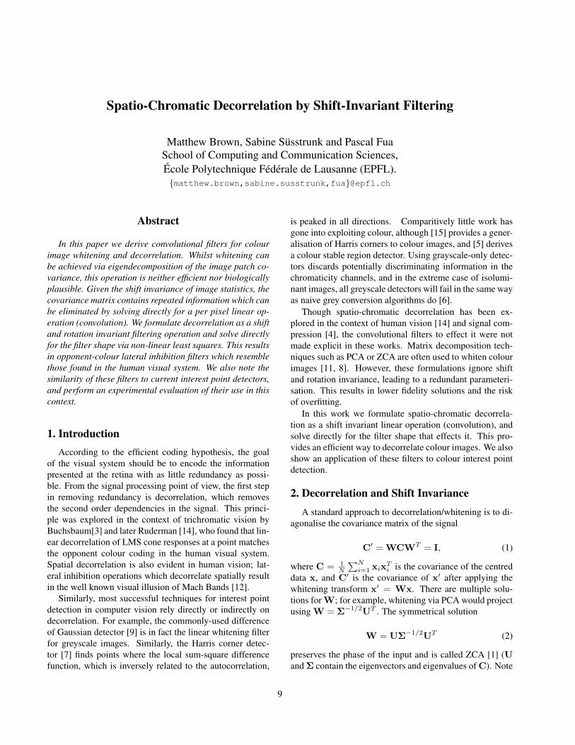
Figure 1: ZCA for colour images. The rows/columns of the symmetric whitening matrix W are shifted versions of each
other (large images), so the whitening transform effectively consists of a convolution with three colour filters (inset images).
that one can also decorrelate without whitening by multipli-
cation by UT . The results of applying ZCA to a colour
image covariance matrix sampled from 106 pixels in 1000
images [10] are shown in Figure 1. The three larger im-
ages visualise the rows/columns of W. As can be seen, the
columns are all shifted versions of each other, so that mul-
tiplication by the whitening matrix W is effectively a con-
volution with the 3 colour filters shown in the inset images.
This structure is not explicitly enforced, but arises because
of the shift invariance of image statistics. This motivated us
to explicitly look for a shift-invariant linear operation (i.e.,
a convolution), that whitens colour images.
In addition to shift invariance, images also have rota-
tion and scale invariance. The scale invariance of image
statistics is well known [13], and is observed for example
in the power law distribution of amplitude spectra, A(ω) ∝1/ω. Rotation invariance may not be exactly present in all
cases, for example, human authored images of man-made
scenes have more energy in the horizontal and vertical di-
rections [16]. However, human images of natural scenes
are almost rotation invariant, and rotation invariance is also
a desirable property in many matching applications, so we
will enforce it here also.
Given shift, rotation and scale invariance, the second or-
der statistics may be encapsulated in a 1-dimensional auto-
correlation function, which measures the similarity of pixels
in any direction, at any scale and at any position. Formulat-
ing our whitening filters as 1-dimensional functions will al-
low us to use a reduced parametrisation, helping to prevent
overfitting, and we will also be able to handle longer range
correlations than possible with PCA/ZCA (e.g. computing
ZCA on 64x64 colour image patches requires factorisation
of a 36,864×36,864 matrix).
2.1. Spatial Decorrelation and DOG
We can whiten a shift-invariant signal I(x) by convolv-
ing with a filter h(x) such that the autocorrelation of the
output equals the dirac delta function. We start by comput-
ing the image autocorrelation function, by sampling the im-
age in a straight line at random positions, orientations and
scales
rI(τ) =1
N
N∑
k=1
Ik(x)Ik(x + τ). (3)
Ik(x) represents the image sampled at a random position,
orientation and scale. This is represented for a greyscale
image in Figure 2, leftmost plot. We then find the inverse
filter h(x) which satisfies
rI(x) ∗ rh(x) = δ(x) (4)
where δ(x) is the unit impulse, and rh(x) = h(x) ∗ h(x) is
the autocorrelation of the filter. Equivalently
PI(ω)PH(ω) = 1 (5)
where PI(ω) is the power spectrum of the signal (Fourier
transform of the autocorrelation) and PH(ω) is the power
spectrum of the filter. One could compute H(ω) and thus
h(x) by inverting the square root of the power spectrum,
with suitable priors on the high frequency components of
h(x). Instead, we choose to solve Equation 4 directly in the
spatial domain, solving for the whitening filter with mini-
mum squared intensity error for a smoothed pulse output
h∗(x) = minh(x)
∑
x
|rI(x) ∗ (h(x) ∗ h(x)) − p(x)|2
+ λ∑
x
(ρ(x)h(x))2 . (6)
We relax the requirement of complete decorrelation by set-
ting p(x) = g(x; 0, σ2), with a small σ of around 4 pixels.
h(x) is constrained to be symmetric i.e., h(−x) = h(x),and we apply a weighting ρ(x) that encourages h(x) to
fall to zero as x becomes large (we have used ρ(x) =(1+(2x/nh)2) where nh is the size of the filter). Equation 6
is solved using standard non-linear least squares solvers and
converges well from any random initialisation.
10

−60 −40 −20 0 20 40 600.55
0.6
0.65
0.7
0.75
0.8
0.85
0.9
0.95
1
1.05
pixels−60 −40 −20 0 20 40 60
−0.4
−0.2
0
0.2
0.4
0.6
0.8
1
pixels−200 −150 −100 −50 0 50 100 150 200
−0.2
0
0.2
0.4
0.6
0.8
1
1.2
pixels
target
actual
−60 −40 −20 0 20 40 60
−0.4
−0.2
0
0.2
0.4
0.6
0.8
1
pixels−200 −150 −100 −50 0 50 100 150 200
−0.2
0
0.2
0.4
0.6
0.8
1
1.2
pixels
target
actual
Figure 2: Greyscale decorrelation. The difference of Gaussian filter is an effective decorrelation filter for greyscale images.
We solve for a whitening filter (centre-left) that converts the long range image correlations (top-left) to leave only residual
correlations with nearby pixels (centre-right). Adding a prior on the energy and spatial extent of the result gives a DOG like
function (top-right), with less ringing than the unsmoothed version (bottom-right).
The solution is visualised in Figure 2. The image is
convolved with a symmetric filter (centre-left column), so
that the target output autocorrelation is a smoothed pulse
(centre-right column). The solution is well modelled by a
difference of Gaussian function. This result provides some
justification as to why the popular difference of Gaussian
operation (used for example in SIFT [9]) might be a good
one in early image understanding, e.g., interest point detec-
tors – it decorrelates a greyscale input image.
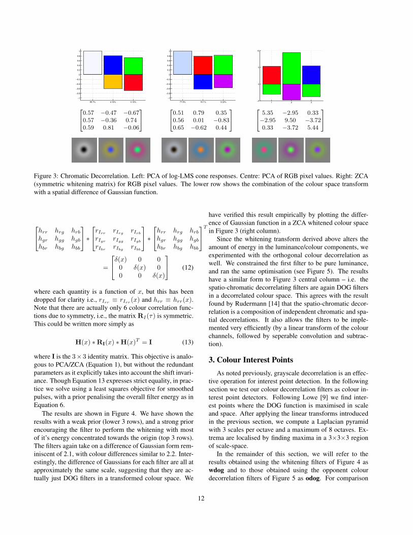
2.2. Chromatic Decorrelation and OpponentColours
The RGB colour channels are also strongly correlated,
with overall changes in intensity affecting each channel al-
most equally and making up the majority of the signal en-
ergy. The eigenvectors of the colour correlation matrix also
have strong connection to human vision, as pointed out by
Buchsbaum [3]. If we represent the colour information us-
ing the theoretical LMS (long, medium, short wavelength)
cone responses, the principal components correspond to lu-
minance (≈95% energy), and the opponent chrominance
channels of blue-yellow and red-green (see Figure 3, left).
The eigenvectors of sRGB images are slightly different (see
Figure 3). A smaller, but still large fraction (80%) of
the energy is in an achromatic channel, with colour differ-
ences of red-blue and green-purple making up the remain-
ing decorrelated channels. These results were computed us-
ing 1000+ calibrated images from the McGill Colour Image
Database [10].
The rightmost plot in Figure 3 shows the zero-phase
whitening matrix W = UΣ−1/2
UT for the sRGB colour
channels. Note that there are multiple whitening transforms,
corresponding to arbitrary rotations of this matrix.
2.3. Combining Spatial and Chromatic Decorrelation
After having found whitening operations for spatial and
chromatic dimensions separately, it seems natural to inves-
tigate the joint objective, i.e., to find a decorrelating filter
for both space and chromaticity togther. In this case, the
whitening is achieved via convolution with a matrix func-
tion
I′(x) = H(x) ∗ I(x) (7)
so that each whitened output in I′ =
[
r′ g′ b′]
is the
convolution of 3 channel colour filter (one row of H(x))with the input (∗ denotes matrix convolution), i.e.,
r′(x)g′(x)b′(x)
=
hrr(x) hrg(x) hrb(x)hgr(x) hgg(x) hgb(x)hbr(x) hbg(x) hbb(x)
∗
r(x)g(x)b(x)
. (8)
The whitened image autocorrelation function is
RI′(τ) = E(
I′(x)I′(x + τ)T
)
(9)
= E(
H(x) ∗ I(x) . I(x + τ)T ∗ H(x)T)
(10)
= H(x) ∗ RI(τ) ∗ H(x)T (11)
Thus for whitening of the output we require
11
95.7% 4.16% 0.16%
−1
−0.8
−0.6
−0.4
−0.2
0
0.2
0.4
0.6
0.8
1
77.9% 19.1% 3.02%
−1
−0.8
−0.6
−0.4
−0.2
0
0.2
0.4
0.6
0.8
1
1 2 3−5
0
5
10
2
4
0.57 −0.47 −0.67
0.57 −0.36 0.74
0.59 0.81 −0.06
3
5
2
4
0.51 0.79 0.35
0.56 0.01 −0.83
0.65 −0.62 0.44
3
5
2
4
5.35 −2.95 0.33
−2.95 9.50 −3.72
0.33 −3.72 5.44
3
5
Figure 3: Chromatic Decorrelation. Left: PCA of log-LMS cone responses. Centre: PCA of RGB pixel values. Right: ZCA
(symmetric whitening matrix) for RGB pixel values. The lower row shows the combination of the colour space transform
with a spatial difference of Gaussian function.
hrr hrg hrb
hgr hgg hgb
hbr hbg hbb
∗
rIrrrIrg
rIrb
rIgrrIgg
rIgb
rIbrrIbg
rIbb
∗
hrr hrg hrb
hgr hgg hgb
hbr hbg hbb
T
=
δ(x) 0 00 δ(x) 00 0 δ(x)
(12)
where each quantity is a function of x, but this has been
dropped for clarity i.e., rIrr≡ rIrr
(x) and hrr ≡ hrr(x).Note that there are actually only 6 colour correlation func-
tions due to symmetry, i.e., the matrix RI(τ) is symmetric.
This could be written more simply as
H(x) ∗ RI(x) ∗ H(x)T = I (13)
where I is the 3× 3 identity matrix. This objective is analo-
gous to PCA/ZCA (Equation 1), but without the redundant
parameters as it explicitly takes into account the shift invari-
ance. Though Equation 13 expresses strict equality, in prac-
tice we solve using a least squares objective for smoothed
pulses, with a prior penalising the overall filter energy as in
Equation 6.
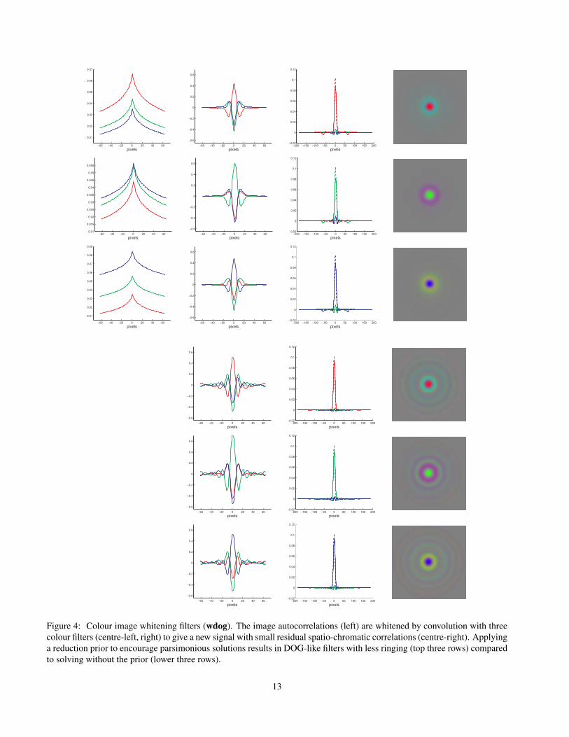
The results are shown in Figure 4. We have shown the
results with a weak prior (lower 3 rows), and a strong prior
encouraging the filter to perform the whitening with most
of it’s energy concentrated towards the origin (top 3 rows).
The filters again take on a difference of Gaussian form rem-
iniscent of 2.1, with colour differences similar to 2.2. Inter-
estingly, the difference of Gaussians for each filter are all at
approximately the same scale, suggesting that they are ac-
tually just DOG filters in a transformed colour space. We
have verified this result empirically by plotting the differ-
ence of Gaussian function in a ZCA whitened colour space
in Figure 3 (right column).
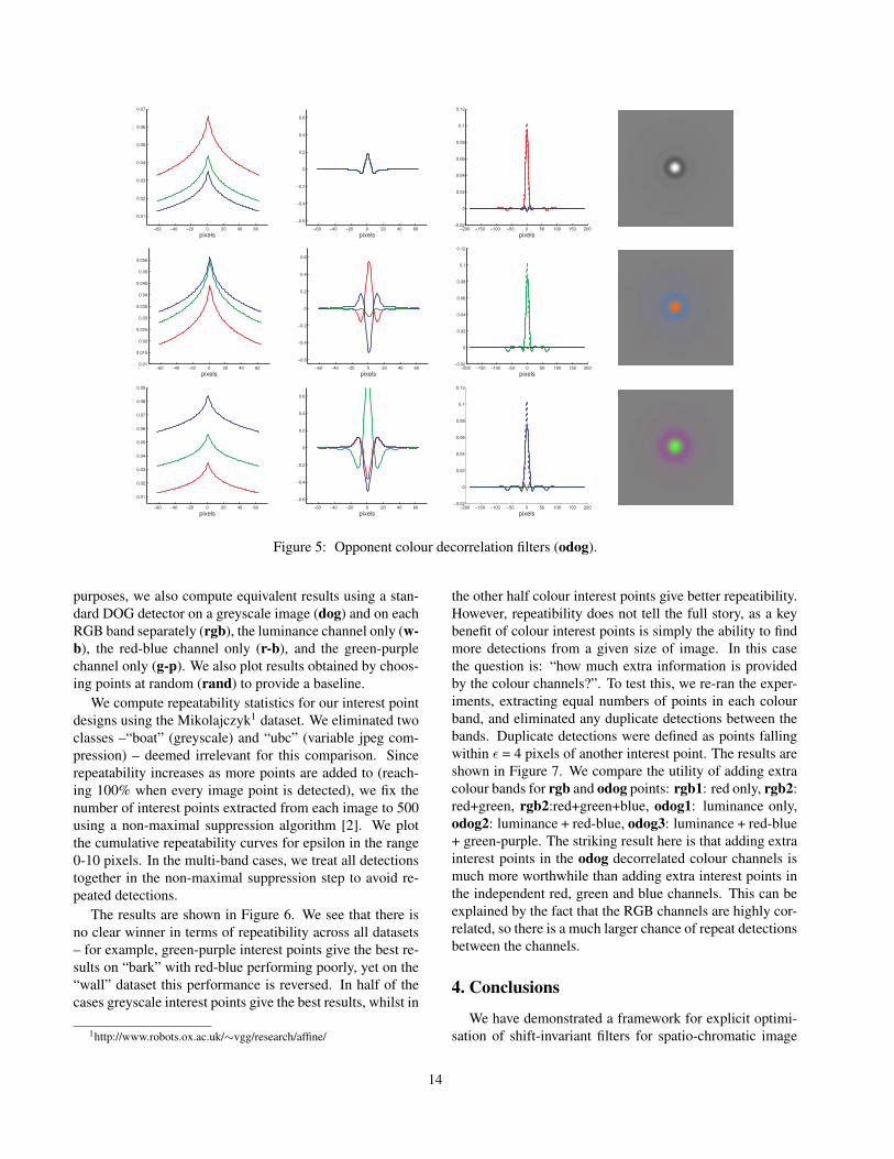
Since the whitening transform derived above alters the
amount of energy in the luminance/colour components, we
experimented with the orthogonal colour decorrelation as
well. We constrained the first filter to be pure luminance,
and ran the same optimisation (see Figure 5). The results
have a similar form to Figure 3 central column – i.e. the
spatio-chromatic decorrelating filters are again DOG filters
in a decorrelated colour space. This agrees with the result
found by Rudermann [14] that the spatio-chromatic decor-
relation is a composition of independent chromatic and spa-
tial decorrelations. It also allows the filters to be imple-
mented very efficiently (by a linear transform of the colour
channels, followed by seperable convolution and subtrac-
tion).
3. Colour Interest Points
As noted previously, grayscale decorrelation is an effec-
tive operation for interest point detection. In the following
section we test our colour decorrelation filters as colour in-
terest point detectors. Following Lowe [9] we find inter-
est points where the DOG function is maximised in scale
and space. After applying the linear transforms introduced
in the previous section, we compute a Laplacian pyramid
with 3 scales per octave and a maximum of 8 octaves. Ex-
trema are localised by finding maxima in a 3×3×3 region
of scale-space.
In the remainder of this section, we will refer to the
results obtained using the whitening filters of Figure 4 as
wdog and to those obtained using the opponent colour
decorrelation filters of Figure 5 as odog. For comparison
12
−60 −40 −20 0 20 40 60
0.01
0.02
0.03
0.04
0.05
0.06
0.07
pixels−60 −40 −20 0 20 40 60
−0.6
−0.4
−0.2
0
0.2
0.4
0.6
pixels−200 −150 −100 −50 0 50 100 150 200
−0.02
0
0.02
0.04
0.06
0.08
0.1
0.12
pixels
−60 −40 −20 0 20 40 600.01
0.015
0.02
0.025
0.03
0.035
0.04
0.045
0.05
0.055
pixels−60 −40 −20 0 20 40 60
−0.6
−0.4
−0.2
0
0.2
0.4
0.6
pixels−200 −150 −100 −50 0 50 100 150 200
−0.02
0
0.02
0.04
0.06
0.08
0.1
0.12
pixels
−60 −40 −20 0 20 40 60
0.01
0.02
0.03
0.04
0.05
0.06
0.07
0.08
0.09
pixels−60 −40 −20 0 20 40 60
−0.6
−0.4
−0.2
0
0.2
0.4
0.6
pixels−200 −150 −100 −50 0 50 100 150 200
−0.02
0
0.02
0.04
0.06
0.08
0.1
0.12
pixels
−60 −40 −20 0 20 40 60
−0.6
−0.4
−0.2
0
0.2
0.4
0.6
pixels−200 −150 −100 −50 0 50 100 150 200
−0.02
0
0.02
0.04
0.06
0.08
0.1
0.12
pixels
−60 −40 −20 0 20 40 60
−0.6
−0.4
−0.2
0
0.2
0.4
0.6
pixels−200 −150 −100 −50 0 50 100 150 200
−0.02
0
0.02
0.04
0.06
0.08
0.1
0.12
pixels
−60 −40 −20 0 20 40 60
−0.6
−0.4
−0.2
0
0.2
0.4
0.6
pixels−200 −150 −100 −50 0 50 100 150 200
−0.02
0
0.02
0.04
0.06
0.08
0.1
0.12
pixels
Figure 4: Colour image whitening filters (wdog). The image autocorrelations (left) are whitened by convolution with three
colour filters (centre-left, right) to give a new signal with small residual spatio-chromatic correlations (centre-right). Applying
a reduction prior to encourage parsimonious solutions results in DOG-like filters with less ringing (top three rows) compared
to solving without the prior (lower three rows).
13
−60 −40 −20 0 20 40 60
0.01
0.02
0.03
0.04
0.05
0.06
0.07
pixels−60 −40 −20 0 20 40 60
−0.6
−0.4
−0.2
0
0.2
0.4
0.6
pixels−200 −150 −100 −50 0 50 100 150 200
−0.02
0
0.02
0.04
0.06
0.08
0.1
0.12
pixels
−60 −40 −20 0 20 40 600.01
0.015
0.02
0.025
0.03
0.035
0.04
0.045
0.05
0.055
pixels−60 −40 −20 0 20 40 60
−0.6
−0.4
−0.2
0
0.2
0.4
0.6
pixels−200 −150 −100 −50 0 50 100 150 200
−0.02
0
0.02
0.04
0.06
0.08
0.1
0.12
pixels
−60 −40 −20 0 20 40 60
0.01
0.02
0.03
0.04
0.05
0.06
0.07
0.08
0.09
pixels−60 −40 −20 0 20 40 60
−0.6
−0.4
−0.2
0
0.2
0.4
0.6
pixels−200 −150 −100 −50 0 50 100 150 200
−0.02
0
0.02
0.04
0.06
0.08
0.1
0.12
pixels
Figure 5: Opponent colour decorrelation filters (odog).
purposes, we also compute equivalent results using a stan-
dard DOG detector on a greyscale image (dog) and on each
RGB band separately (rgb), the luminance channel only (w-
b), the red-blue channel only (r-b), and the green-purple
channel only (g-p). We also plot results obtained by choos-
ing points at random (rand) to provide a baseline.
We compute repeatability statistics for our interest point
designs using the Mikolajczyk1 dataset. We eliminated two
classes –“boat” (greyscale) and “ubc” (variable jpeg com-
pression) – deemed irrelevant for this comparison. Since
repeatability increases as more points are added to (reach-
ing 100% when every image point is detected), we fix the
number of interest points extracted from each image to 500
using a non-maximal suppression algorithm [2]. We plot
the cumulative repeatability curves for epsilon in the range
0-10 pixels. In the multi-band cases, we treat all detections
together in the non-maximal suppression step to avoid re-
peated detections.
The results are shown in Figure 6. We see that there is
no clear winner in terms of repeatibility across all datasets
– for example, green-purple interest points give the best re-
sults on “bark” with red-blue performing poorly, yet on the
“wall” dataset this performance is reversed. In half of the
cases greyscale interest points give the best results, whilst in
1http://www.robots.ox.ac.uk/∼vgg/research/affine/
the other half colour interest points give better repeatibility.
However, repeatibility does not tell the full story, as a key
benefit of colour interest points is simply the ability to find
more detections from a given size of image. In this case
the question is: “how much extra information is provided
by the colour channels?”. To test this, we re-ran the exper-
iments, extracting equal numbers of points in each colour
band, and eliminated any duplicate detections between the
bands. Duplicate detections were defined as points falling
within ǫ = 4 pixels of another interest point. The results are
shown in Figure 7. We compare the utility of adding extra
colour bands for rgb and odog points: rgb1: red only, rgb2:
red+green, rgb2:red+green+blue, odog1: luminance only,
odog2: luminance + red-blue, odog3: luminance + red-blue
+ green-purple. The striking result here is that adding extra
interest points in the odog decorrelated colour channels is
much more worthwhile than adding extra interest points in
the independent red, green and blue channels. This can be
explained by the fact that the RGB channels are highly cor-
related, so there is a much larger chance of repeat detections
between the channels.
4. Conclusions
We have demonstrated a framework for explicit optimi-
sation of shift-invariant filters for spatio-chromatic image
14

0 2 4 6 8 100
10
20
30
40
50
60
epsilon/pixels
rep
ea
tib
ility
/pe
rce
nt
dog
odog
w−b
r−b
g−p
wdog
rgb
rand
0 2 4 6 8 100
10
20
30
40
50
60
epsilon/pixels
rep
ea
tib
ility
/pe
rce
nt
dog
odog
w−b
r−b
g−p
wdog
rgb
rand
0 2 4 6 8 100
10
20
30
40
50
epsilon/pixels
rep
ea
tib
ility
/pe
rce
nt
dog
odog
w−b
r−b
g−p
wdog
rgb
rand
0 2 4 6 8 100
10
20
30
40
50
60
epsilon/pixels
rep
ea
tib
ility
/pe
rce
nt
dog
odog
w−b
r−b
g−p
wdog
rgb
rand
0 2 4 6 8 100
10
20
30
40
50
60
epsilon/pixels
rep
ea
tib
ility
/pe
rce
nt
dog
odog
w−b
r−b
g−p
wdog
rgb
rand
0 2 4 6 8 100
10
20
30
40
50
60
70
epsilon/pixels
rep
ea
tib
ility
/pe
rce
nt
dog
odog
w−b
r−b
g−p
wdog
rgb
rand
Figure 6: Repeatability on the Mikolajyzck dataset (left-right, top-bottom: bark, bikes, graffiti, leuven, trees, wall). odog:
orthogonal colour decorrelation filters, wdog: colour whitening filters, dog: greyscale DOG, rgb: DOG on each of RGB
channels, w-b: luminance only, r-b: red-blue, g-p: green-purple, rand: uniform random distributed points. Colour DOG
detectors give equal or better results to greyscale in half of the cases.
0 2 4 6 8 100
1000
2000
3000
4000
5000
epsilon/pixels
nu
mb
er
ma
tch
ed
odog1
odog2
odog3
rgb1
rgb2
rgb3
0 2 4 6 8 100
1000
2000
3000
4000
epsilon/pixels
nu
mb
er
ma
tch
ed
odog1
odog2
odog3
rgb1
rgb2
rgb3
0 2 4 6 8 100
1000
2000
3000
4000
epsilon/pixels
nu
mb
er
ma
tch
ed
odog1
odog2
odog3
rgb1
rgb2
rgb3
0 2 4 6 8 100
1000
2000
3000
4000
5000
epsilon/pixels
nu
mb
er
ma
tch
ed
odog1
odog2
odog3
rgb1
rgb2
rgb3
0 2 4 6 8 100
1000
2000
3000
4000
epsilon/pixels
nu
mb
er
ma
tch
ed
odog1
odog2
odog3
rgb1
rgb2
rgb3
0 2 4 6 8 100
1000
2000
3000
4000
5000
epsilon/pixels
nu
mb
er
ma
tch
ed
odog1
odog2
odog3
rgb1
rgb2
rgb3
Figure 7: Number of independent matches on the Mikolajyzck dataset (left-right, top-bottom: bark, bikes, graffiti, leuven,
trees, wall). rgb1: red only, rgb2: red+green, rgb2: red+green+blue, odog1: luminance only, odog2: luminance + red-blue,
odog3: luminance + red-blue + green-purple. Note that the number of independent matches using the decorellating filters is
far higher than independent DOG filters on RGB.
15
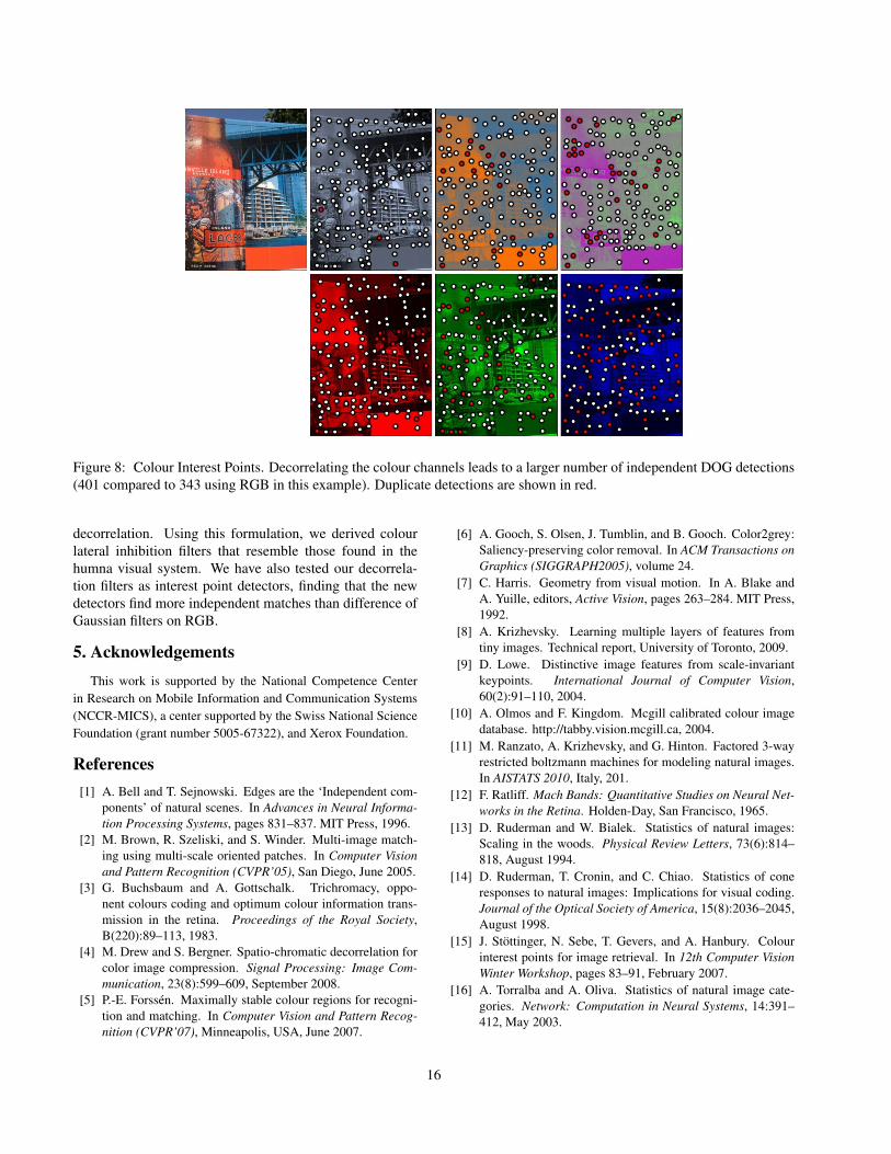
Figure 8: Colour Interest Points. Decorrelating the colour channels leads to a larger number of independent DOG detections
(401 compared to 343 using RGB in this example). Duplicate detections are shown in red.
decorrelation. Using this formulation, we derived colour
lateral inhibition filters that resemble those found in the
humna visual system. We have also tested our decorrela-
tion filters as interest point detectors, finding that the new
detectors find more independent matches than difference of
Gaussian filters on RGB.
5. Acknowledgements
This work is supported by the National Competence Center
in Research on Mobile Information and Communication Systems
(NCCR-MICS), a center supported by the Swiss National Science
Foundation (grant number 5005-67322), and Xerox Foundation.
References
[1] A. Bell and T. Sejnowski. Edges are the ‘Independent com-
ponents’ of natural scenes. In Advances in Neural Informa-
tion Processing Systems, pages 831–837. MIT Press, 1996.
[2] M. Brown, R. Szeliski, and S. Winder. Multi-image match-
ing using multi-scale oriented patches. In Computer Vision
and Pattern Recognition (CVPR’05), San Diego, June 2005.
[3] G. Buchsbaum and A. Gottschalk. Trichromacy, oppo-
nent colours coding and optimum colour information trans-
mission in the retina. Proceedings of the Royal Society,
B(220):89–113, 1983.
[4] M. Drew and S. Bergner. Spatio-chromatic decorrelation for
color image compression. Signal Processing: Image Com-
munication, 23(8):599–609, September 2008.
[5] P.-E. Forssen. Maximally stable colour regions for recogni-
tion and matching. In Computer Vision and Pattern Recog-
nition (CVPR’07), Minneapolis, USA, June 2007.
[6] A. Gooch, S. Olsen, J. Tumblin, and B. Gooch. Color2grey:
Saliency-preserving color removal. In ACM Transactions on
Graphics (SIGGRAPH2005), volume 24.
[7] C. Harris. Geometry from visual motion. In A. Blake and
A. Yuille, editors, Active Vision, pages 263–284. MIT Press,
1992.
[8] A. Krizhevsky. Learning multiple layers of features from
tiny images. Technical report, University of Toronto, 2009.
[9] D. Lowe. Distinctive image features from scale-invariant
keypoints. International Journal of Computer Vision,
60(2):91–110, 2004.
[10] A. Olmos and F. Kingdom. Mcgill calibrated colour image
database. http://tabby.vision.mcgill.ca, 2004.
[11] M. Ranzato, A. Krizhevsky, and G. Hinton. Factored 3-way
restricted boltzmann machines for modeling natural images.
In AISTATS 2010, Italy, 201.
[12] F. Ratliff. Mach Bands: Quantitative Studies on Neural Net-
works in the Retina. Holden-Day, San Francisco, 1965.
[13] D. Ruderman and W. Bialek. Statistics of natural images:
Scaling in the woods. Physical Review Letters, 73(6):814–
818, August 1994.
[14] D. Ruderman, T. Cronin, and C. Chiao. Statistics of cone
responses to natural images: Implications for visual coding.
Journal of the Optical Society of America, 15(8):2036–2045,
August 1998.
[15] J. Stottinger, N. Sebe, T. Gevers, and A. Hanbury. Colour
interest points for image retrieval. In 12th Computer Vision
Winter Workshop, pages 83–91, February 2007.
[16] A. Torralba and A. Oliva. Statistics of natural image cate-
gories. Network: Computation in Neural Systems, 14:391–
412, May 2003.
16
Recommended


![Decorrelation-based Piecewise Digital Predistortion ... · proposed closed-loop learning algorithm is based on a compu-tationally simple decorrelation-based learning rule [10], which](https://img.pdfslide.us/doc/110x75/60349bfa1bd7bc54b93f6fa4/decorrelation-based-piecewise-digital-predistortion-proposed-closed-loop-learning.jpg)