Spacecraft Rendezvous using Chance-ConstrainedModel Predictive Control and ON/OFF thrusters
Rafael Vazquez
Francisco Gavilan Eduardo F. Camacho
Universidad de Sevilla
Workshop on Advances in Space Rendezvous Guidance31 October 2013, Toulouse
IntroductionMPC applied to Rendezvous
ON/OFF thrusters
MPCRendezvous model, Constraints, Cost Function
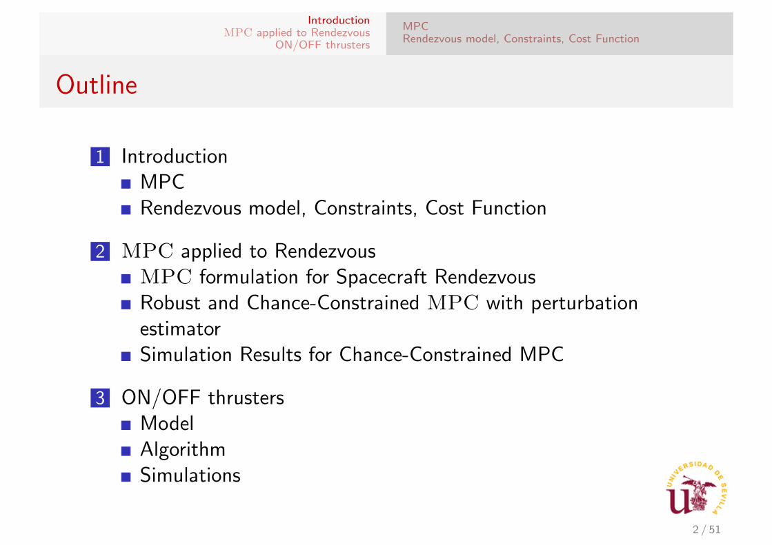
Outline
1 IntroductionMPCRendezvous model, Constraints, Cost Function
2 MPC applied to RendezvousMPC formulation for Spacecraft RendezvousRobust and Chance-Constrained MPC with perturbationestimatorSimulation Results for Chance-Constrained MPC
3 ON/OFF thrustersModelAlgorithmSimulations
2 / 51
IntroductionMPC applied to Rendezvous
ON/OFF thrusters
MPCRendezvous model, Constraints, Cost Function
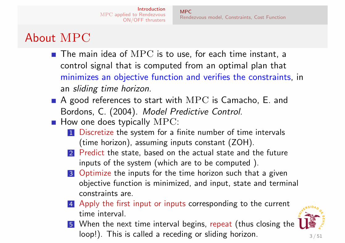
About MPCThe main idea of MPC is to use, for each time instant, acontrol signal that is computed from an optimal plan thatminimizes an objective function and verifies the constraints, inan sliding time horizon.A good references to start with MPC is Camacho, E. andBordons, C. (2004). Model Predictive Control.How one does typically MPC:
1 Discretize the system for a finite number of time intervals(time horizon), assuming inputs constant (ZOH).
2 Predict the state, based on the actual state and the futureinputs of the system (which are to be computed ).
3 Optimize the inputs for the time horizon such that a givenobjective function is minimized, and input, state and terminalconstraints are.
4 Apply the first input or inputs corresponding to the currenttime interval.
5 When the next time interval begins, repeat (thus closing theloop!). This is called a receding or sliding horizon. 3 / 51
IntroductionMPC applied to Rendezvous
ON/OFF thrusters
MPCRendezvous model, Constraints, Cost Function
LTI example. Discretization.
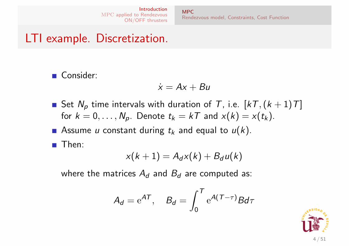
Consider:x = Ax + Bu
Set Np time intervals with duration of T , i.e. [kT , (k + 1)T ]for k = 0, . . . ,Np. Denote tk = kT and x(k) = x(tk).
Assume u constant during tk and equal to u(k).
Then:x(k + 1) = Adx(k) + Bdu(k)
where the matrices Ad and Bd are computed as:
Ad = eAT , Bd =
∫ T
0eA(T−τ)Bdτ
4 / 51
IntroductionMPC applied to Rendezvous
ON/OFF thrusters
MPCRendezvous model, Constraints, Cost Function
LTI example. Prediction of the state.
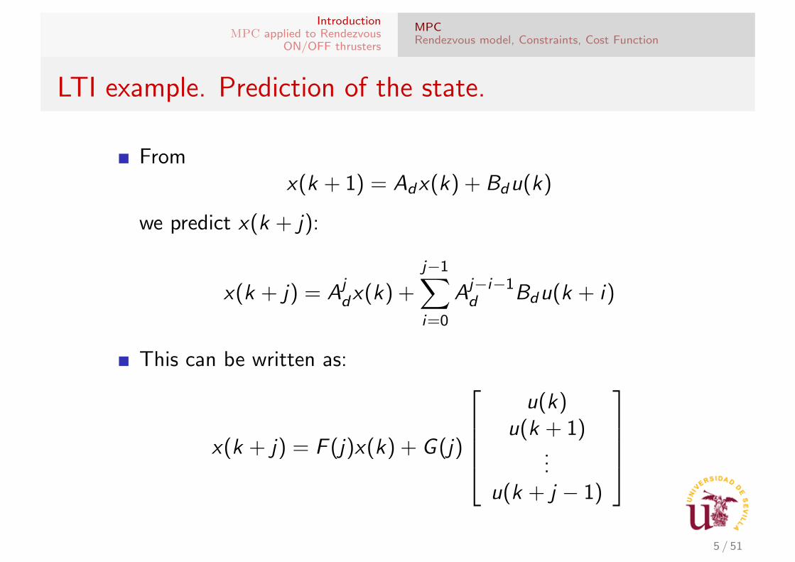
Fromx(k + 1) = Adx(k) + Bdu(k)
we predict x(k + j):
x(k + j) = Ajdx(k) +
j−1∑i=0
Aj−i−1d Bdu(k + i)
This can be written as:
x(k + j) = F (j)x(k) + G (j)
u(k)
u(k + 1)...
u(k + j − 1)
5 / 51

IntroductionMPC applied to Rendezvous
ON/OFF thrusters
MPCRendezvous model, Constraints, Cost Function
LTI example. Optimization.
Given inequality constraints
∀k ∈ [0,Np − 1], Aix(k) ≤ bi , Auu ≤ bu
and terminal constraints Atx(Np) = bt .
Given an objective function J(x , u) to minimize over a finitehorizon K ∈ [0,Np].
If we know x(0), all constraints can be put in terms of u(0),. . ., u(Np − 1).
Since the inputs are a discrete, finite set → finite-dimensionaloptimization problem. Easily solvable if the objective functionis quadratic or linear!
6 / 51
IntroductionMPC applied to Rendezvous
ON/OFF thrusters
MPCRendezvous model, Constraints, Cost Function
LTI example. Receding horizon
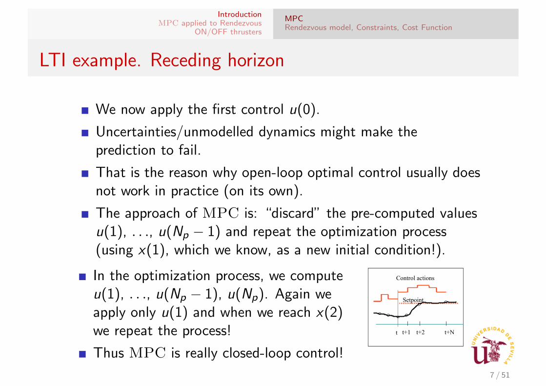
We now apply the first control u(0).
Uncertainties/unmodelled dynamics might make theprediction to fail.
That is the reason why open-loop optimal control usually doesnot work in practice (on its own).
The approach of MPC is: “discard” the pre-computed valuesu(1), . . ., u(Np − 1) and repeat the optimization process(using x(1), which we know, as a new initial condition!).
In the optimization process, we computeu(1), . . ., u(Np − 1), u(Np). Again weapply only u(1) and when we reach x(2)we repeat the process!
Thus MPC is really closed-loop control!
t t+1 t+2 t+N
Control actions
Setpoint
7 / 51

IntroductionMPC applied to Rendezvous
ON/OFF thrusters
MPCRendezvous model, Constraints, Cost Function
A guidance example: first step
t t+1 t+2
t+N t t+1 t+2 !!.. t+N
u(t)
Only the first control move is applied
Errors minimized over a finite horizon
Constraints taken into account
Model of process used for predicting
8 / 51
IntroductionMPC applied to Rendezvous
ON/OFF thrusters
MPCRendezvous model, Constraints, Cost Function
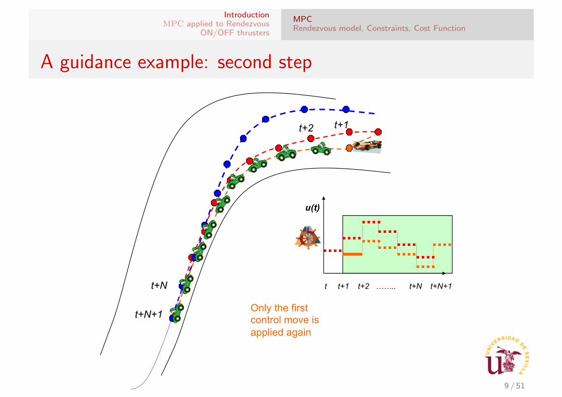
A guidance example: second step
t+2 t+1
t+N
t+N+1
t t+1 t+2 !!.. t+N t+N+1
u(t)
Only the first control move is applied again
9 / 51
IntroductionMPC applied to Rendezvous
ON/OFF thrusters
MPCRendezvous model, Constraints, Cost Function
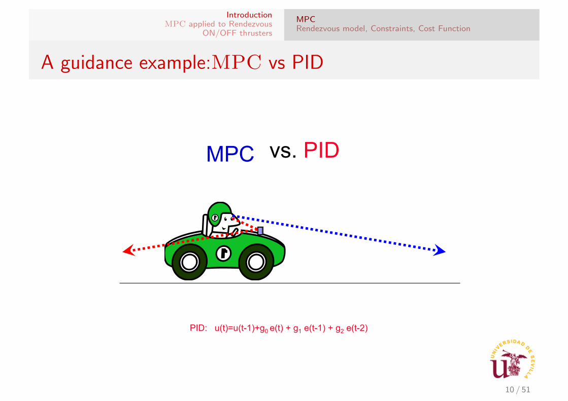
A guidance example:MPC vs PID
MPC
PID: u(t)=u(t-1)+g0 e(t) + g1 e(t-1) + g2 e(t-2)
vs. PID
10 / 51
IntroductionMPC applied to Rendezvous
ON/OFF thrusters
MPCRendezvous model, Constraints, Cost Function
Advantages and Disadvantages of MPC
Advantages: it looks into the future, it is optimal, it can treatmany type of constraints, it guarantees a good performance ofthe system. It can also consider disturbances!
Disadvantages: hard for nonlinear systems, requires some timefor optimal input computation.
It has been widely used in real life, for instance in chemicalplants (there are companies specializing in MPC).
However now that computational resources are cheap andmore powerful, MPC is emerging as a feasible technique formany applications, for instance in the aerospace field.
Spacecraft rendezvous is an excellent example, since it isvery well described by linear equations and it is a slow system.
11 / 51
IntroductionMPC applied to Rendezvous
ON/OFF thrusters
MPCRendezvous model, Constraints, Cost Function
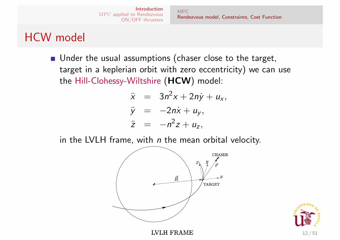
HCW model
Under the usual assumptions (chaser close to the target,target in a keplerian orbit with zero eccentricity) we can usethe Hill-Clohessy-Wiltshire (HCW) model:
x = 3n2x + 2ny + ux ,
y = −2nx + uy ,
z = −n2z + uz ,
in the LVLH frame, with n the mean orbital velocity.
12 / 51
IntroductionMPC applied to Rendezvous
ON/OFF thrusters
MPCRendezvous model, Constraints, Cost Function
Constraints of the problem
Typical constraints:
Thruster limitations and mode of operation (PWM or PAM).Avoid collisions between chaser and target (safety).Typically, chaser must approach inside a previously designatedsafe zone.If there are chaser engine failures, rendezvous should still beachieved, if possible (fault tolerant control).If the target’s attitude is changing with time (spinning target)the chaser should couple with that rotation to still guaranteerendezvous.In case of total failure, collision probability should be as smallas possible.
Such constraints should be satisfied at the same time thatfuel consumption is optimized (economy).
13 / 51
IntroductionMPC applied to Rendezvous
ON/OFF thrusters
MPCRendezvous model, Constraints, Cost Function
Safe zone
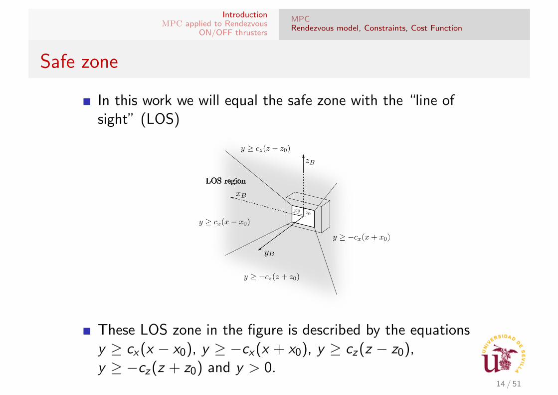
In this work we will equal the safe zone with the “line ofsight” (LOS)
These LOS zone in the figure is described by the equationsy ≥ cx(x − x0), y ≥ −cx(x + x0), y ≥ cz(z − z0),y ≥ −cz(z + z0) and y > 0.
14 / 51
IntroductionMPC applied to Rendezvous
ON/OFF thrusters
MPCRendezvous model, Constraints, Cost Function
Actuator constraints and Cost Function
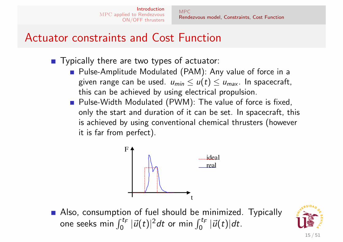
Typically there are two types of actuator:Pulse-Amplitude Modulated (PAM): Any value of force in agiven range can be used. umin ≤ u(t) ≤ umax . In spacecraft,this can be achieved by using electrical propulsion.Pulse-Width Modulated (PWM): The value of force is fixed,only the start and duration of it can be set. In spacecraft, thisis achieved by using conventional chemical thrusters (howeverit is far from perfect).
Spacecraft Attitude Dynamics and Control Course notes
35
Actuators for spacecraft attitude control
Thrusters for attitude control
The simplest way to create torques is to create a set of forces with direction not aligned with the center of mass, and this can be obtained by mass expulsion techniques. Jet thrusters pose some operational problems due to the ignition transient, and besides it is not simple to finely control the magnitude of the force, so these devices are not used for fine attitude control. In addition, for control quite often the force needed is rather small (milli Newton-meters), while chemical thrusters produce forces in the order of at least some Newton. To make them compatible with attitude control, they are switched on and off with a given modulation, but this enhances the problems due to ignition transients and can cause mechanical ware of the thruster. These problems can be solved by adopting electric propulsion thrusters, based on electrodynamic acceleration of a suitable ionized propellant, that need de-ionization immediately after expulsion to avoid charging electrically the spacecraft. These thrusters can be easily modulated in amplitude, have a high specific impulse (over 3000) that allows a reduced propellant consumption. The thrust produced can be in the order of a few Newton down to 10-6 Newton, so they are well suited to fine control actions. Unfortunately, electric thrusters are extremely power consuming, more or less 90% is devoted simply to keep it ready to use and only 10% is due to the thrust produced, therefore electric propulsion units are often coupled to extremely large solar panels. With conventional (chemical) thrusters it is not possible to control the amplitude of the thrust; they are either switched on or off. The transient delay and the presence of hydraulic circuits make the actual thrust profile quite different from the ideal one, requiring a careful calibration for proper command selection.
F ideal real t
Use of thruster on spinned satellites In case of spinning satellites, to control the spin velocity the thrusters must be located on the side of the satellite and the thrust direction must be orthogonal to the angular velocity:
MI =ω!
Also, consumption of fuel should be minimized. Typicallyone seeks min
∫ tF0 |~u(t)|2dt or min
∫ tF0 |~u(t)|dt.
15 / 51

IntroductionMPC applied to Rendezvous
ON/OFF thrusters
MPC formulation for Spacecraft RendezvousRobust and Chance-Constrained MPC with perturbation estimatorSimulation Results for Chance-Constrained MPC
HCW model in discrete time with perturbations
Assuming that the control signal is constant for each samplingtime T , we obtain the following discrete time version of theHCW equations:
x(k + 1) = ATx(k) + BTu(k) + δ(k).
AT and BT are:
AT =
4− 3C 0 0 Sn
2(1−C)n
0
6(S − nT ) 1 0 − 2(1−C)n
4S−3nTn
0
0 0 C 0 0 Sn
3nS 0 0 C 2S 0−6n(1− C) 0 0 −2S 4C − 3 0
0 0 −nS 0 0 C
BT =
1−C
n22nT−2S
n2 0
2(S−nT )
n2 − 3T2
2+ 4 1−C
n2 0
0 0 1−C
n2Sn
2 1−Cn
02(C−1)
n−3T + 4 S
n0
0 0 Sn
where S = sin nT y C = cos nT (T = 60 s is used in this
work). We will drop the subindex T in AT and BT .16 / 51

IntroductionMPC applied to Rendezvous
ON/OFF thrusters
MPC formulation for Spacecraft RendezvousRobust and Chance-Constrained MPC with perturbation estimatorSimulation Results for Chance-Constrained MPC
State, perturbation and control variables
x(k), u(k) y δ(k) denote respectively the state (position andvelocity), control effort (propulsive force per unit mass) andperturbation for time t = k , where:
x = [x y z x y z ]T , u = [ux uy uz ]T ,
δ = [δx δy δz δx δy δz ]T .
x , y , and z are position in the LVLH local frame about thecenter of gravity of the target.
x is radial position, y is position along the orbit and z isperpendicular to the orbit.
Velocity, control u(k) and perturbations δ(k) are also writtenin the LVLH frame.
Perturbations are unknown, hence δ(k) is a 6-D randomvariable, of mean δ and covariance matrix Σ also unknown.
17 / 51
IntroductionMPC applied to Rendezvous
ON/OFF thrusters
MPC formulation for Spacecraft RendezvousRobust and Chance-Constrained MPC with perturbation estimatorSimulation Results for Chance-Constrained MPC
Prediction of state and compact notation
The state at t = k + j is predicted from the past state x(k)and control and disturbances at times from t = k to timet = k + j − 1 as:
x(k + j) = Ajx(k) +
j−1∑i=0
Aj−i−1Bu(k + i) +
j−1∑i=0
Aj−i−1δ(k + i).
We use a compact (stack) notation where we denote:
xS(k) =
x(k + 1)x(k + 2)
.
.
.x(k + Np)
, uS(k) =
u(k)
u(k + 1)
.
.
.u(k + Np − 1)
, δS(k) =
δ(k)
δ(k + 1)
.
.
.δ(k + Np − 1)
.
Hence we can write the prediction equations as:
xS(k) = Fx(k) + GuuS(k) + GδδS(k),
where F, Gu and Gδ are defined from the model matricesA and B.
18 / 51
IntroductionMPC applied to Rendezvous
ON/OFF thrusters
MPC formulation for Spacecraft RendezvousRobust and Chance-Constrained MPC with perturbation estimatorSimulation Results for Chance-Constrained MPC
Constraints
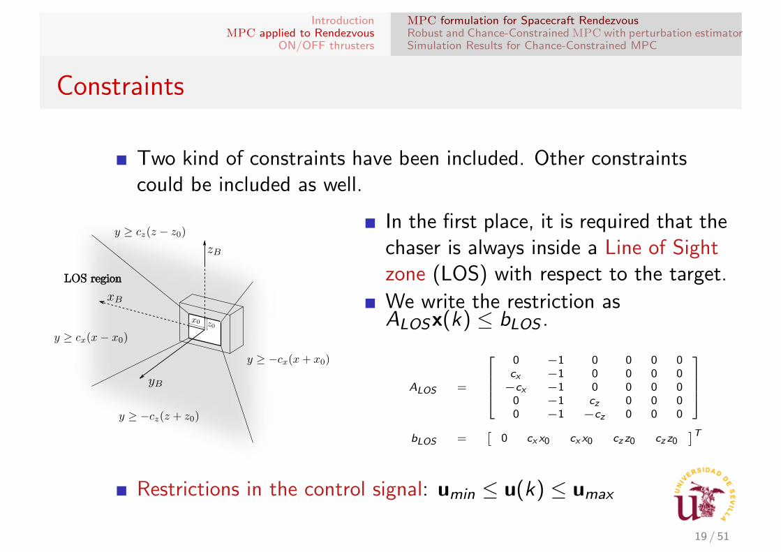
Two kind of constraints have been included. Other constraintscould be included as well.
In the first place, it is required that thechaser is always inside a Line of Sightzone (LOS) with respect to the target.
We write the restriction asALOSx(k) ≤ bLOS .
ALOS =
0 −1 0 0 0 0cx −1 0 0 0 0−cx −1 0 0 0 0
0 −1 cz 0 0 00 −1 −cz 0 0 0
bLOS =
[0 cx x0 cx x0 cz z0 cz z0
]T
Restrictions in the control signal: umin ≤ u(k) ≤ umax
19 / 51

IntroductionMPC applied to Rendezvous
ON/OFF thrusters
MPC formulation for Spacecraft RendezvousRobust and Chance-Constrained MPC with perturbation estimatorSimulation Results for Chance-Constrained MPC
Objective function
Taking expectation we define: x(k + j |k) = E [x(k + j)|x(k)]
Similary xS(k + j |k) = E [xS(k + j)|x(k)].Objective function:
J(k) =
Np∑i=1
[xT (k + i|k)R(k + i)x(k + i|k)
]+
Np∑i=1
[uT (k + i − 1)Qu(k + i − 1)
],
where Np is the control horizon.
Q = Id3×3 and R(k) is defined as:
R(k) = γh(k − ka)
[Id3×3 Θ3×3
Θ3×3 Θ3×3
].
where h is the step function, ka is the desired arrival time andγ is a large number. Hence R = 0 before the arrival time, andafter arrival time it gives a large weight to the error inposition (distance from the origin).
20 / 51
IntroductionMPC applied to Rendezvous
ON/OFF thrusters
MPC formulation for Spacecraft RendezvousRobust and Chance-Constrained MPC with perturbation estimatorSimulation Results for Chance-Constrained MPC
Objective function and constraints in compact notation
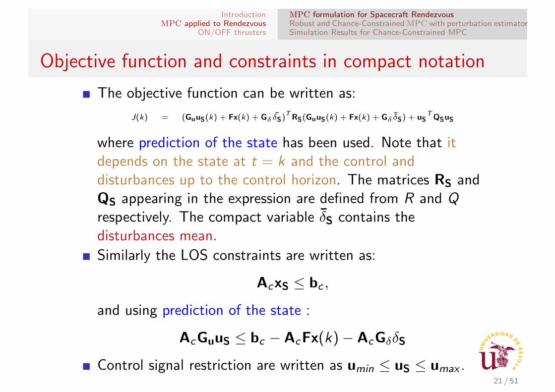
The objective function can be written as:
J(k) = (GuuS(k) + Fx(k) + Gδ δS)T RS(GuuS(k) + Fx(k) + Gδ δS) + uST QSuS
where prediction of the state has been used. Note that itdepends on the state at t = k and the control anddisturbances up to the control horizon. The matrices RS andQS appearing in the expression are defined from R and Qrespectively. The compact variable δS contains thedisturbances mean.
Similarly the LOS constraints are written as:
AcxS ≤ bc ,
and using prediction of the state :
AcGuuS ≤ bc − AcFx(k)− AcGδδS
Control signal restriction are written as umin ≤ uS ≤ umax .21 / 51
IntroductionMPC applied to Rendezvous
ON/OFF thrusters
MPC formulation for Spacecraft RendezvousRobust and Chance-Constrained MPC with perturbation estimatorSimulation Results for Chance-Constrained MPC
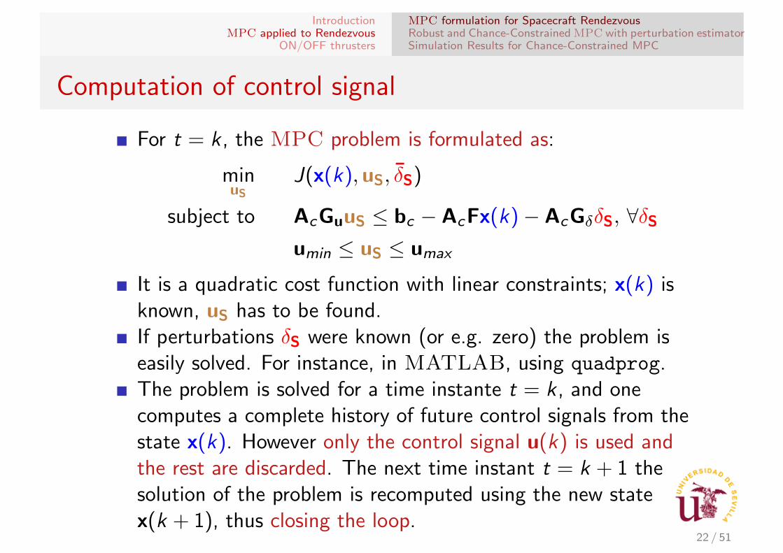
Computation of control signal
For t = k , the MPC problem is formulated as:
minuS
J(x(k),uS, δS)
subject to AcGuuS ≤ bc − AcFx(k)− AcGδδS, ∀δS
umin ≤ uS ≤ umax
It is a quadratic cost function with linear constraints; x(k) isknown, uS has to be found.If perturbations δS were known (or e.g. zero) the problem iseasily solved. For instance, in MATLAB, using quadprog.The problem is solved for a time instante t = k , and onecomputes a complete history of future control signals from thestate x(k). However only the control signal u(k) is used andthe rest are discarded. The next time instant t = k + 1 thesolution of the problem is recomputed using the new statex(k + 1), thus closing the loop.
22 / 51

IntroductionMPC applied to Rendezvous
ON/OFF thrusters
MPC formulation for Spacecraft RendezvousRobust and Chance-Constrained MPC with perturbation estimatorSimulation Results for Chance-Constrained MPC
Robust MPC with known perturbation bounds
If perturbations are unknown, the previous problem is notsolvable.
Assume instead that we just know perturbation bounds:AδδS ≤ cδ (admissible perturbations) and perturbation meansδS.
A control system that achieves its objective for all admissibleperturbations is called robust.
To accommodate all admissible perturbations, we bound−AcGδδS which appears in the minimization constraints, forall admissible perturbations.
This procedure is always possible for bounded perturbations(with known bounds).
23 / 51
IntroductionMPC applied to Rendezvous
ON/OFF thrusters
MPC formulation for Spacecraft RendezvousRobust and Chance-Constrained MPC with perturbation estimatorSimulation Results for Chance-Constrained MPC
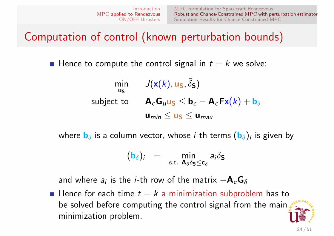
Computation of control (known perturbation bounds)
Hence to compute the control signal in t = k we solve:
minuS
J(x(k),uS, δS)
subject to AcGuuS ≤ bc − AcFx(k) + bδ
umin ≤ uS ≤ umax
where bδ is a column vector, whose i-th terms (bδ)i is given by
(bδ)i = mins.t. AδδS≤cδ
aiδS
and where ai is the i-th row of the matrix −AcGδ
Hence for each time t = k a minimization subproblem has tobe solved before computing the control signal from the mainminimization problem.
24 / 51
IntroductionMPC applied to Rendezvous
ON/OFF thrusters
MPC formulation for Spacecraft RendezvousRobust and Chance-Constrained MPC with perturbation estimatorSimulation Results for Chance-Constrained MPC
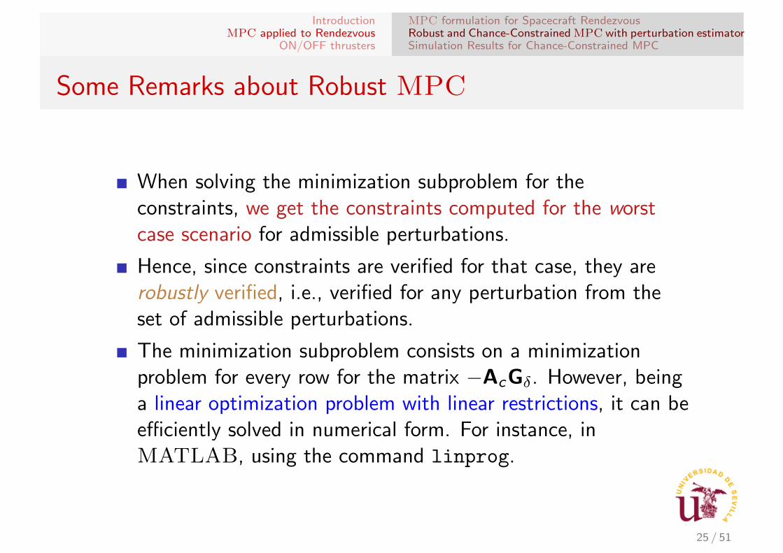
Some Remarks about Robust MPC
When solving the minimization subproblem for theconstraints, we get the constraints computed for the worstcase scenario for admissible perturbations.
Hence, since constraints are verified for that case, they arerobustly verified, i.e., verified for any perturbation from theset of admissible perturbations.
The minimization subproblem consists on a minimizationproblem for every row for the matrix −AcGδ. However, beinga linear optimization problem with linear restrictions, it can beefficiently solved in numerical form. For instance, inMATLAB, using the command linprog.
25 / 51
IntroductionMPC applied to Rendezvous
ON/OFF thrusters
MPC formulation for Spacecraft RendezvousRobust and Chance-Constrained MPC with perturbation estimatorSimulation Results for Chance-Constrained MPC
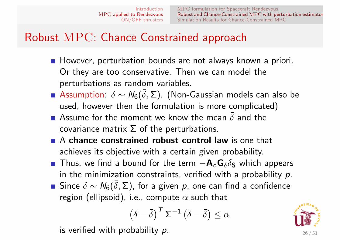
Robust MPC: Chance Constrained approach
However, perturbation bounds are not always known a priori.Or they are too conservative. Then we can model theperturbations as random variables.Assumption: δ ∼ N6(δ,Σ). (Non-Gaussian models can also beused, however then the formulation is more complicated)Assume for the moment we know the mean δ and thecovariance matrix Σ of the perturbations.A chance constrained robust control law is one thatachieves its objective with a certain given probability.Thus, we find a bound for the term −AcGδδS which appearsin the minimization constraints, verified with a probability p.Since δ ∼ N6(δ,Σ), for a given p, one can find a confidenceregion (ellipsoid), i.e., compute α such that(
δ − δ)T
Σ−1(δ − δ
)≤ α
is verified with probability p. 26 / 51
IntroductionMPC applied to Rendezvous
ON/OFF thrusters
MPC formulation for Spacecraft RendezvousRobust and Chance-Constrained MPC with perturbation estimatorSimulation Results for Chance-Constrained MPC
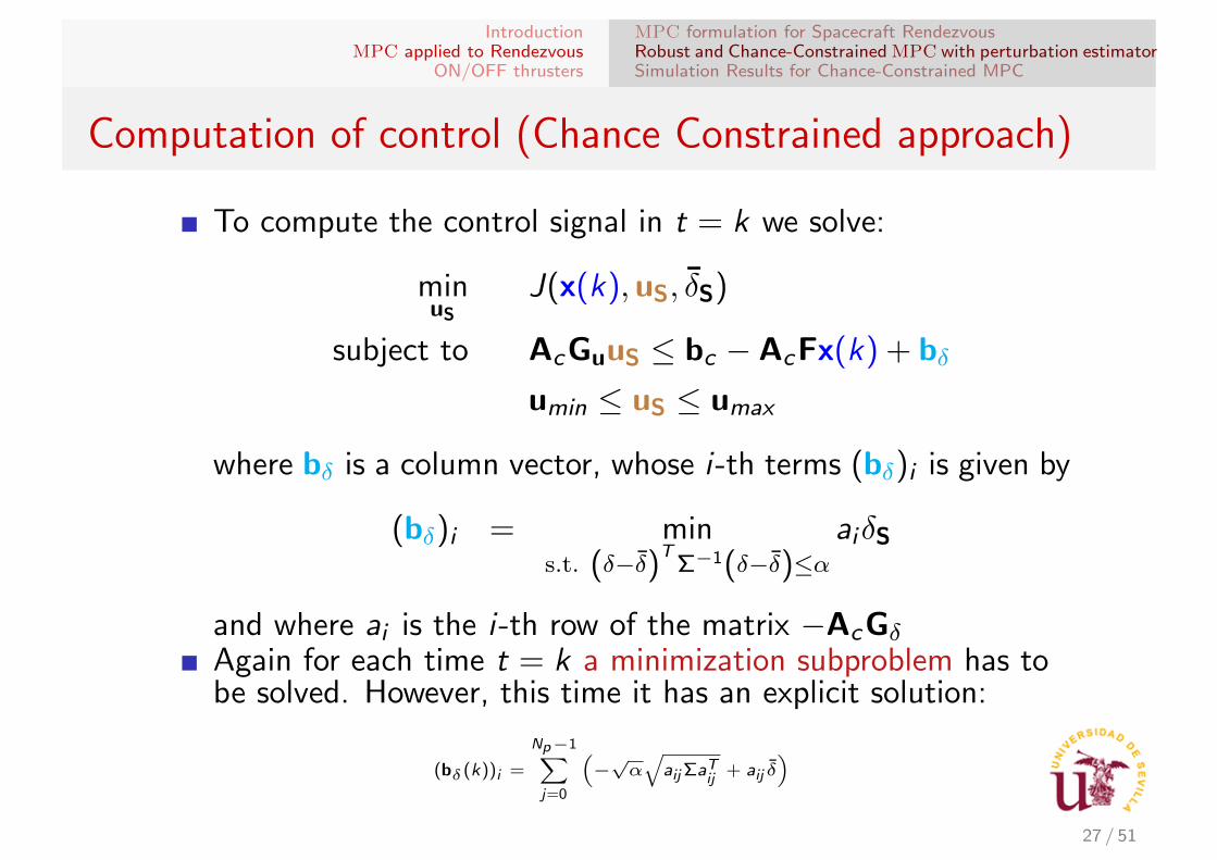
Computation of control (Chance Constrained approach)
To compute the control signal in t = k we solve:
minuS
J(x(k),uS, δS)
subject to AcGuuS ≤ bc − AcFx(k) + bδ
umin ≤ uS ≤ umax
where bδ is a column vector, whose i-th terms (bδ)i is given by
(bδ)i = mins.t. (δ−δ)
TΣ−1(δ−δ)≤α
aiδS
and where ai is the i-th row of the matrix −AcGδ
Again for each time t = k a minimization subproblem has tobe solved. However, this time it has an explicit solution:
(bδ(k))i =
Np−1∑j=0
(−√α√
aijΣaTij + aij δ)
27 / 51
IntroductionMPC applied to Rendezvous
ON/OFF thrusters
MPC formulation for Spacecraft RendezvousRobust and Chance-Constrained MPC with perturbation estimatorSimulation Results for Chance-Constrained MPC
Some Remarks about the Chance Constrained approach
Since the minimization subproblem is explicitly solved, thisapproach gives an algorithm as fast as the non-robust MPC.
However:
Needs estimation of statistical properties.The normal distribution is unbounded: cannot choose theprobability p of constraint satisfaction too large:conservativeness or even unfeasibility.Each constraint satisfied with probability p: global probabilitysmaller. However compensated with the receding horizon ofMPC!
28 / 51

IntroductionMPC applied to Rendezvous
ON/OFF thrusters
MPC formulation for Spacecraft RendezvousRobust and Chance-Constrained MPC with perturbation estimatorSimulation Results for Chance-Constrained MPC
Algorithm for estimating perturbations
The Chance Constrained Robust MPC, as it has beenformulated, requires knowing the mean and covariance of theperturbations.
Frequently, perturbations are totally unknown and these datahas to be obtained online using an estimator.
Then, for each t = k we estimate δ y Σ taking into accountpast perturbations, using:
δ(i) = x(i + 1)− Ax(i)− Bu(i),
for i = 1, . . . , k − 1.
29 / 51
IntroductionMPC applied to Rendezvous
ON/OFF thrusters
MPC formulation for Spacecraft RendezvousRobust and Chance-Constrained MPC with perturbation estimatorSimulation Results for Chance-Constrained MPC
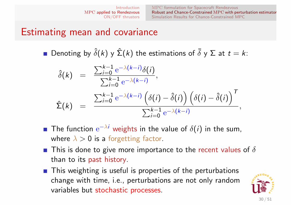
Estimating mean and covariance
Denoting by δ(k) y Σ(k) the estimations of δ y Σ at t = k :
δ(k) =
∑k−1i=0 e−λ(k−i)δ(i)∑k−1
i=0 e−λ(k−i),
Σ(k) =
∑k−1i=0 e−λ(k−i)
(δ(i)− δ(i)
)(δ(i)− δ(i)
)T∑k−1
i=0 e−λ(k−i),
The function e−λi weights in the value of δ(i) in the sum,where λ > 0 is a forgetting factor.
This is done to give more importance to the recent values of δthan to its past history.
This weighting is useful is properties of the perturbationschange with time, i.e., perturbations are not only randomvariables but stochastic processes.
30 / 51
IntroductionMPC applied to Rendezvous
ON/OFF thrusters
MPC formulation for Spacecraft RendezvousRobust and Chance-Constrained MPC with perturbation estimatorSimulation Results for Chance-Constrained MPC
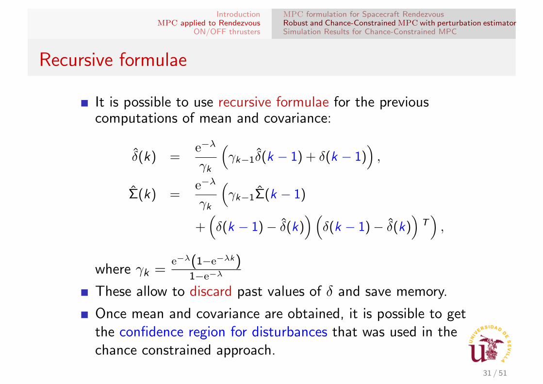
Recursive formulae
It is possible to use recursive formulae for the previouscomputations of mean and covariance:
δ(k) =e−λ
γk
(γk−1δ(k − 1) + δ(k − 1)
),
Σ(k) =e−λ
γk
(γk−1Σ(k − 1)
+(δ(k − 1)− δ(k)
)(δ(k − 1)− δ(k)
)T),
where γk =e−λ(1−e−λk)
1−e−λ
These allow to discard past values of δ and save memory.
Once mean and covariance are obtained, it is possible to getthe confidence region for disturbances that was used in thechance constrained approach.
31 / 51
IntroductionMPC applied to Rendezvous
ON/OFF thrusters
MPC formulation for Spacecraft RendezvousRobust and Chance-Constrained MPC with perturbation estimatorSimulation Results for Chance-Constrained MPC
Simulations
For numerical simulations, several scenarios have beenconsidered with and without perturbations.
Parameters used: R0 = 6878 km, n = 1.1068 · 10−3 rad/s, andLOS constraint parameters: x0 = z0 = 1.5m and cx = cz = 1.
We included propulsive perturbations in the form:ureal = (1 + δ1)T (δθ)u, where:
ureal is the real control signal given by the propulsive system.u is the computed (desired) control signal.δ1 is a normally distributed random variable. Physically, δ1
represents errors in the actuators.T (δθ) is a rotation matrix with rotation angles given by δθ,which is a normally distributed random vector of (small)angles. Physically, it comes from small errors in attitude thatcause the engines to be slightly off course.
Much more complex than nominal model.
32 / 51

IntroductionMPC applied to Rendezvous
ON/OFF thrusters
MPC formulation for Spacecraft RendezvousRobust and Chance-Constrained MPC with perturbation estimatorSimulation Results for Chance-Constrained MPC
Non-robust MPC controller
Good results without perturbations (solid line).
Fails when perturbations are present (dashed line). Howeverif perturbations are small, still works.
33 / 51
IntroductionMPC applied to Rendezvous
ON/OFF thrusters
MPC formulation for Spacecraft RendezvousRobust and Chance-Constrained MPC with perturbation estimatorSimulation Results for Chance-Constrained MPC
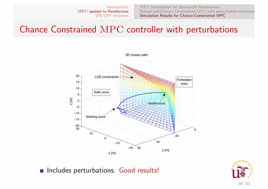
Chance Constrained MPC controller with perturbations
−20
−10
0
10
20 0
20
40
60
−20
−15
−10
−5
0
5
10
15
20
y [m]
3D chaser path
x [m]
z [m
]
Starting point
rendezvous
LOS constraints
Safe zone
Forbiddenarea
Includes perturbations. Good results!
34 / 51
IntroductionMPC applied to Rendezvous
ON/OFF thrusters
MPC formulation for Spacecraft RendezvousRobust and Chance-Constrained MPC with perturbation estimatorSimulation Results for Chance-Constrained MPC
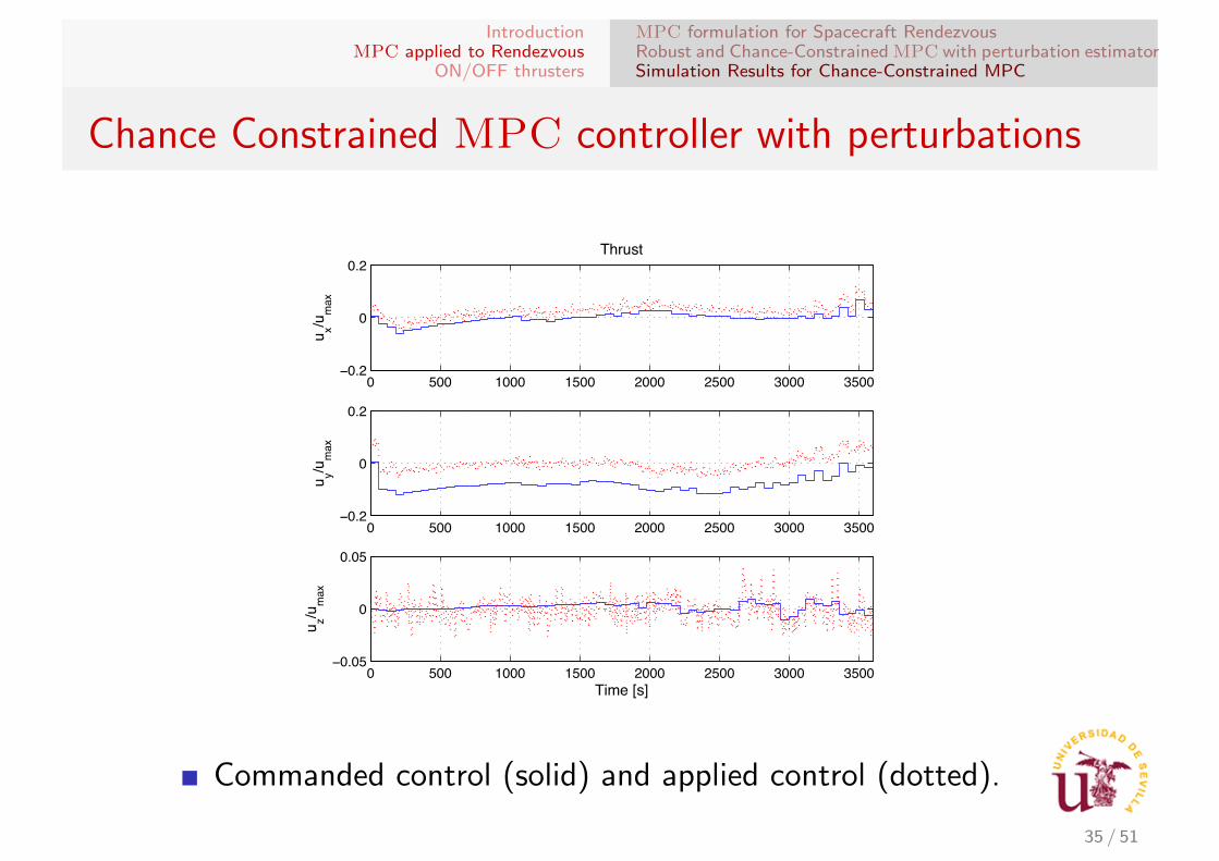
Chance Constrained MPC controller with perturbations
0 500 1000 1500 2000 2500 3000 3500−0.2
0
0.2
u x/um
ax
Thrust
0 500 1000 1500 2000 2500 3000 3500−0.2
0
0.2
u y/um
ax
0 500 1000 1500 2000 2500 3000 3500−0.05
0
0.05
u z/um
ax
Time [s]
Commanded control (solid) and applied control (dotted).
35 / 51

IntroductionMPC applied to Rendezvous
ON/OFF thrusters
MPC formulation for Spacecraft RendezvousRobust and Chance-Constrained MPC with perturbation estimatorSimulation Results for Chance-Constrained MPC
Monte Carlo simulations
Simulated 1220 cases (with different disturbances). For eachcase we perform a simulation with the non-robust and anotherwith the robust (chance constrained) approach.
In the table d is the relative distance at the desired arrivaltime.
Non-robust MPC Robust MPC
Constraint violations 59% 0%
d ≤ 0.2m 19% 100%
0.2m ≤ d ≤ 0.5m 22% 0%
0.5m ≤ d 0% 0%
Mean cost (m/s) ofsuccessful missions
0.2444 0.2039
36 / 51
IntroductionMPC applied to Rendezvous
ON/OFF thrusters
MPC formulation for Spacecraft RendezvousRobust and Chance-Constrained MPC with perturbation estimatorSimulation Results for Chance-Constrained MPC
Monte Carlo simulations
0 0.5 1 1.5
x 10−4
0.05
0.1
0.15
0.2
0.25
0.3
0.35
0.4
0.45
| δ1
|
Mis
sion
cos
t [m
/s]
Robust MPC
Non−robust MPC
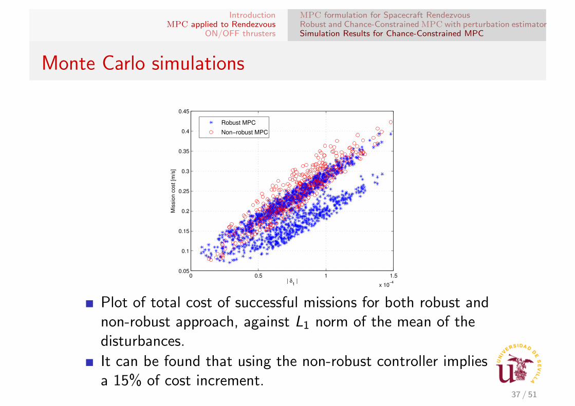
Plot of total cost of successful missions for both robust andnon-robust approach, against L1 norm of the mean of thedisturbances.
It can be found that using the non-robust controller impliesa 15% of cost increment.
37 / 51
IntroductionMPC applied to Rendezvous
ON/OFF thrusters
MPC formulation for Spacecraft RendezvousRobust and Chance-Constrained MPC with perturbation estimatorSimulation Results for Chance-Constrained MPC
Monte Carlo simulations
0 0.5 1 1.5
x 10−4
−0.04
−0.02
0
0.02
0.04
0.06
0.08
0.1
0.12
| �1 |
1 [m/s]
Mis
sion
cos
t diff
eren
ce [m
/s]
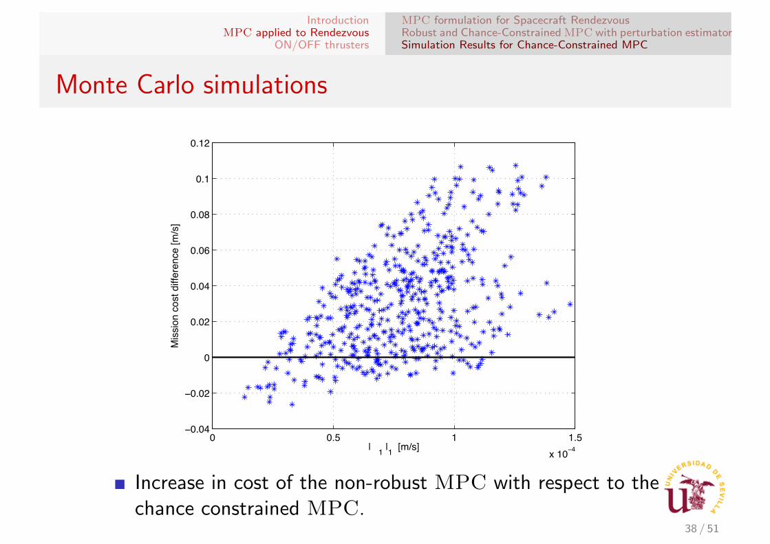
Increase in cost of the non-robust MPC with respect to thechance constrained MPC.
38 / 51
IntroductionMPC applied to Rendezvous
ON/OFF thrusters
MPC formulation for Spacecraft RendezvousRobust and Chance-Constrained MPC with perturbation estimatorSimulation Results for Chance-Constrained MPC
Non-robust MPC controller with unmodeled dynamics
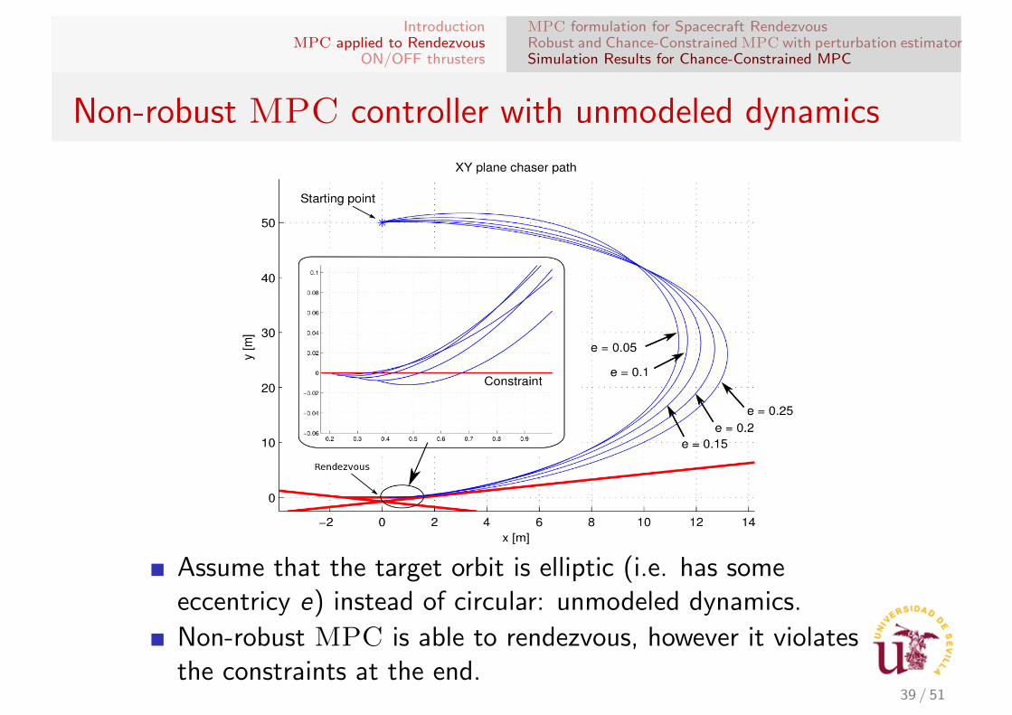
Assume that the target orbit is elliptic (i.e. has someeccentricy e) instead of circular: unmodeled dynamics.
Non-robust MPC is able to rendezvous, however it violatesthe constraints at the end.
39 / 51
IntroductionMPC applied to Rendezvous
ON/OFF thrusters
MPC formulation for Spacecraft RendezvousRobust and Chance-Constrained MPC with perturbation estimatorSimulation Results for Chance-Constrained MPC
Robust MPC controller with unmodeled dynamics
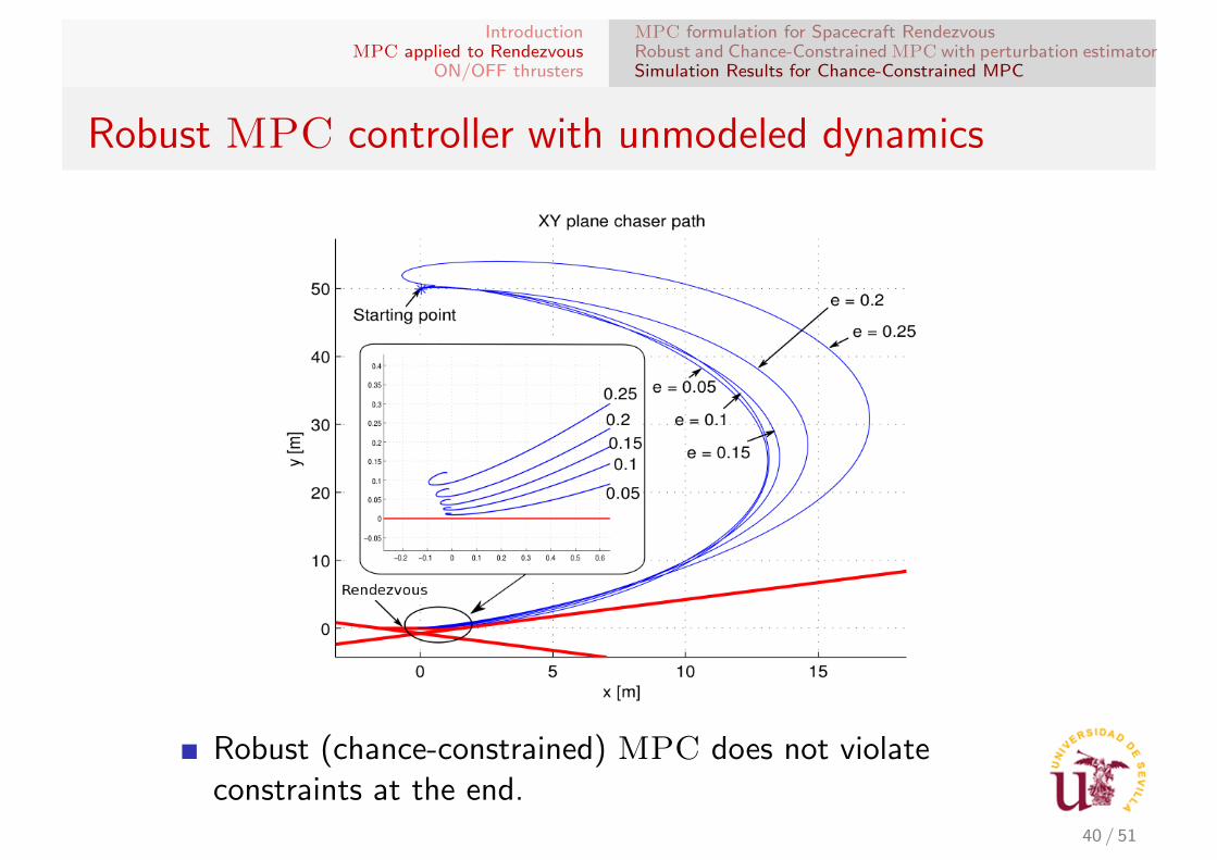
Robust (chance-constrained) MPC does not violateconstraints at the end.
40 / 51
IntroductionMPC applied to Rendezvous
ON/OFF thrusters
MPC formulation for Spacecraft RendezvousRobust and Chance-Constrained MPC with perturbation estimatorSimulation Results for Chance-Constrained MPC
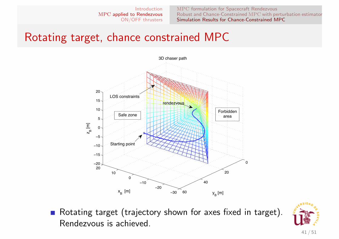
Rotating target, chance constrained MPC
−30−20
−100
1020
0
20
40
60
−20
−15
−10
−5
0
5
10
15
20
yB [m]
3D chaser path
xB [m]
z B [m
]
Safe zoneForbidden
area
LOS constraints
rendezvous
Starting point
Rotating target (trajectory shown for axes fixed in target).Rendezvous is achieved.
41 / 51
IntroductionMPC applied to Rendezvous
ON/OFF thrusters
ModelAlgorithmSimulations
Rendezvous with ON/OFF thrusters
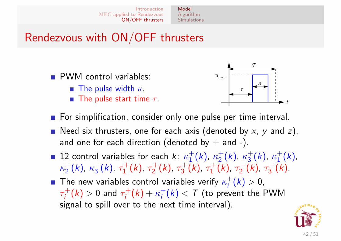
PWM control variables:
The pulse width κ.The pulse start time τ .
maxu
t
T
·¿
For simplification, consider only one pulse per time interval.
Need six thrusters, one for each axis (denoted by x , y and z),and one for each direction (denoted by + and -).
12 control variables for each k : κ+1 (k), κ+
2 (k), κ+3 (k), κ+
1 (k),κ−2 (k), κ−3 (k), τ+
1 (k), τ+2 (k), τ+
3 (k), τ+1 (k), τ−2 (k), τ−3 (k).
The new variables control variables verify κ+i (k) > 0,
τ+i (k) > 0 and τ+
i (k) + κ+i (k) < T (to prevent the PWM
signal to spill over to the next time interval).
42 / 51
IntroductionMPC applied to Rendezvous
ON/OFF thrusters
ModelAlgorithmSimulations
Rendezvous with ON/OFF thrusters: model
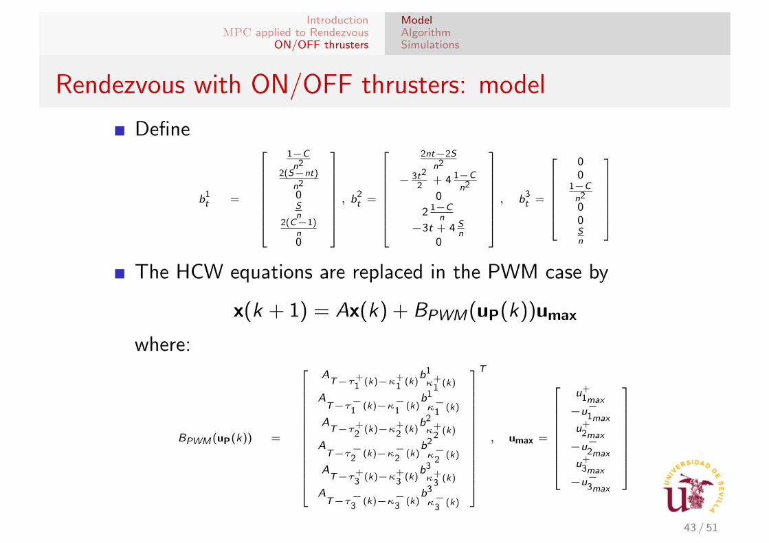
Define
b1t =
1−C
n22(S−nt)
n2
0Sn
2(C−1)n0
, b2
t =
2nt−2S
n2
− 3t2
2+ 4 1−C
n2
0
2 1−Cn
−3t + 4 Sn
0
, b3
t =
00
1−C
n2
00Sn
The HCW equations are replaced in the PWM case by
x(k + 1) = Ax(k) + BPWM(uP(k))umax
where:
BPWM (uP(k)) =
AT−τ+
1(k)−κ+
1(k)
b1
κ+1
(k)
AT−τ
−1
(k)−κ−1
(k)b1
κ−1
(k)
AT−τ+
2(k)−κ+
2(k)
b2
κ+2
(k)
AT−τ
−2
(k)−κ−2
(k)b2
κ−2
(k)
AT−τ+
3(k)−κ+
3(k)
b3
κ+3
(k)
AT−τ
−3
(k)−κ−3
(k)b3
κ−3
(k)
T
, umax =
u+1max−u−1maxu+
2max−u−2maxu+
3max−u−3max
43 / 51
IntroductionMPC applied to Rendezvous
ON/OFF thrusters
ModelAlgorithmSimulations
Rendezvous with ON/OFF thrusters: model
The equations are highly nonlinear in the control!
The procedure with PAM control cannot be applied. We uselinearization, applying the following algorithm:
1 Solve the problem using the normal algorithm for PAM control.2 Use the optimal PAM-PWM filter to get a initial starting guess
of the PWM solution (see next slide).3 Linearize around the actual PWM solution and find small
increments in the PWM controls that improve the objectivefunction and satisfy the constraints.
4 Repeat previous step until it converges or time is up.
Linearization is explicit and easy to compute (since thematrices come from a discretized continuous system).
Since we have a very good initial guess the algorithm workswell.
44 / 51
IntroductionMPC applied to Rendezvous
ON/OFF thrusters
ModelAlgorithmSimulations
Optimal PAM-PWM filter
Since we are linearizing it is crucial to have a good initialguess.
The optimal PAM-PWM filter is an algorithm that takes asequence of PAM control inputs and produces a sequence ofPWM control inputs, such that both system outputs are veryclose.
Found in the literature: e.g. Shieh et al, “Design of PAM andPWM controllers for sampled-data interval systems,” J DynSyst Meas Contr., 118.
Simple and system independent, works specially well for linearsystems. Based on two rules:
The law of areas: both PWM and PAM control inputs mustproduce, for each sample interval, the same area.The pulse (when there is only one) must be centered in thesample interval.
45 / 51
IntroductionMPC applied to Rendezvous
ON/OFF thrusters
ModelAlgorithmSimulations
Linearization of the PWM model
The linearized model is written as
x(k + 1) = Ax(k) + BPWM(uP(k))umax + B∆(uP(k))∆(k)
∆(k) are the increments in the PWM signals and the matrixB∆(uP(k)) is defined explicitly as:
B∆=
−A′T−τ+
1−κ+
1
b1
κ+1
u+1max(
−A′T−τ+
1−κ+
1
b1
κ+1
+ AT−τ+
1−κ+
1b1′κ+
1
)u+
1max
.
.
.(A′T−τ
−3−κ−3
b3
κ−3
− AT−τ
−3−κ−3
b3′
κ−3
)u−3max
T
,
In the matrix, A′t = ddtAt , b
i ′t = d
dt bit .
Since the model is now linear, optimization is fast (even inMatlab!).
46 / 51

IntroductionMPC applied to Rendezvous
ON/OFF thrusters
ModelAlgorithmSimulations
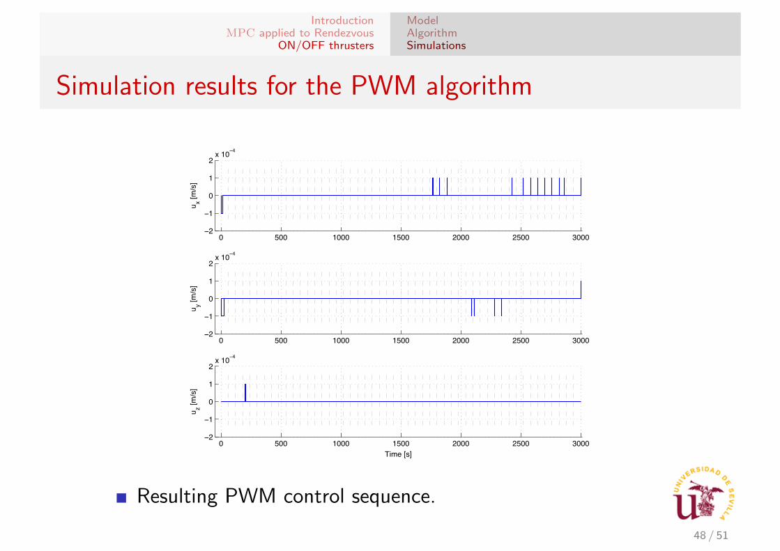
Simulation results for the PWM algorithm
−50 0 50 100 150 200 250 300 350
0
100
200
300
400
500
600
700
x [m]
y[m
]
PAM/PWM FilterLOS RestrictionIteration #1Iteration #2Iteration #3Iteration #4
Rendezvous
LOS Restriction
Starting point
Comparison between a PAM and PWM trajectory applyingthe algorithm. Without disturbances.
47 / 51
IntroductionMPC applied to Rendezvous
ON/OFF thrusters
ModelAlgorithmSimulations
Simulation results for the PWM algorithm
0 500 1000 1500 2000 2500 3000−2
−1
0
1
2x 10
−4
u x [m/s
]
0 500 1000 1500 2000 2500 3000−2
−1
0
1
2x 10
−4
u y [m/s
]
0 500 1000 1500 2000 2500 3000−2
−1
0
1
2x 10
−4
u z [m/s
]
Time [s]
Resulting PWM control sequence.
48 / 51

IntroductionMPC applied to Rendezvous
ON/OFF thrusters
ModelAlgorithmSimulations
Simulation results for the PWM algorithm
0 1 2 3 4 5 6 7 8 9 105.1
5.15
5.2
5.25
5.3x 10
−3
# of Iterations
Cos
t fun
ctio
n [m
/s]
Interpolated valuePAM/PWM FilterPWM Iterations
Improvement in the cost function for each iteration.
After 5-6 iterations, it converges.
Slight improvement in cost.49 / 51
Conclusions
We have presented a robust MPC controller to solve theproblem of automatic spacecraft rendezvous.Perturbations are estimated online and accommodated.In simulations it is shown that the method can overcome largedisturbance and unmodeled dynamics.PWM control constraints have been included in the model.Future work:
Include eccentricity and orbital perturbations.Add an state estimator (based e.g. on observations fromtarget).Include fault-tolerant schemes and safety constraints.Use more sophisticated disturbance estimation techniques.Study stability of the closed loop system.Reduce # of actuators, include attitude dynamics (nonlinear).
References:1 F. Gavilan, R. Vazquez, E. F. Camacho, “Robust Model Predictive Control for Spacecraft
Rendezvous with Online Prediction of Disturbance Bounds,” IFAC AGNFCS‘09, Samara, Russia,2009.
2 R. Vazquez, F. Gavilan, E. F. Camacho, “Trajectory Planning for Spacecraft Rendezvous withOn/Off Thrusters,” IFAC World Congress, 2011.
3 F. Gavilan, R. Vazquez and E. F. Camacho,“Chance-constrained Model Predictive Control forSpacecraft Rendezvous with Disturbance Estimation,” Control Engineering Practice, 20 (2),111-122, 2012.

Thankyou!
http://aero.us.es/rvazquez/research.htm
Recommended


![Rendezvous of Non-Cooperative Spacecraft and Tug … dynamics is carried out assuming that the tether’s ... Many modern spacecraft are equipped with de-orbiting facilities [24-27]](https://img.pdfslide.us/doc/110x75/5b3229c27f8b9a2c328d2347/rendezvous-of-non-cooperative-spacecraft-and-tug-dynamics-is-carried-out-assuming.jpg)