Sorting (Part II)
CSE 373Data Structures
Sorting (prt II) 2
How fast can we sort?
• Heapsort, Mergesort, and Quicksort all run in O(N log N) best case running time
• Can we do any better?• No, if sorting is comparison-based.
Sorting (prt II) 3
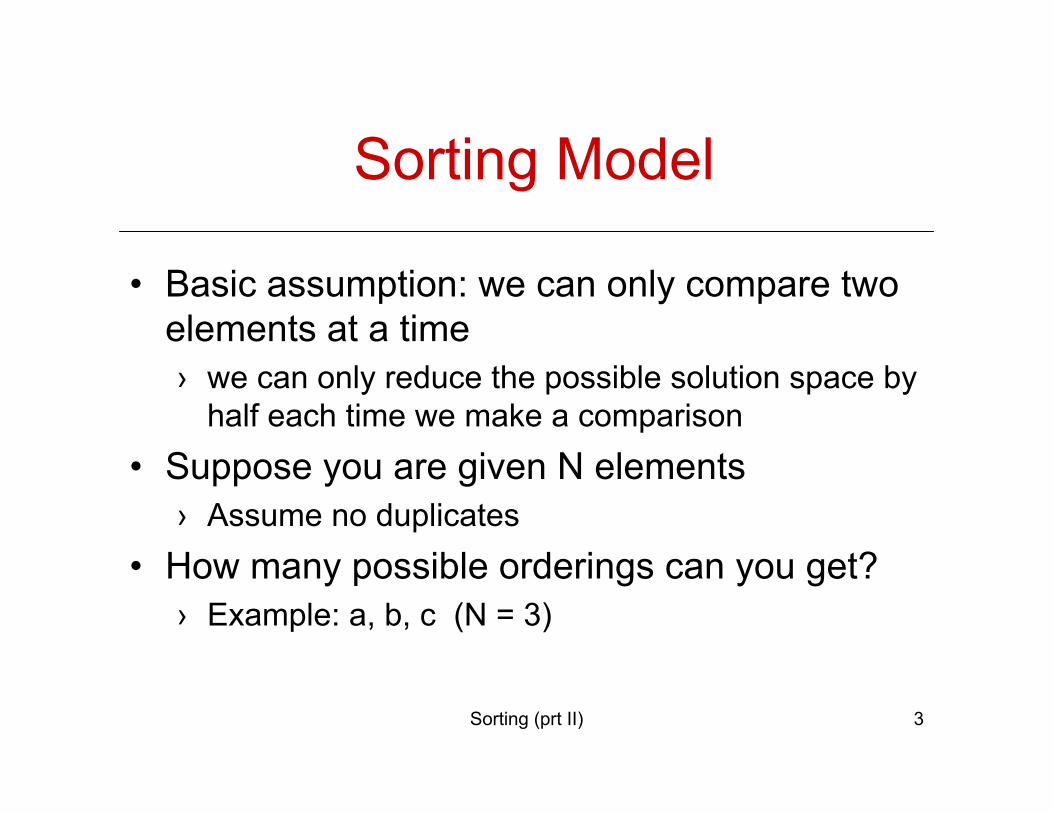
Sorting Model
• Basic assumption: we can only compare two elements at a time › we can only reduce the possible solution space by
half each time we make a comparison• Suppose you are given N elements
› Assume no duplicates• How many possible orderings can you get?
› Example: a, b, c (N = 3)
Sorting (prt II) 4
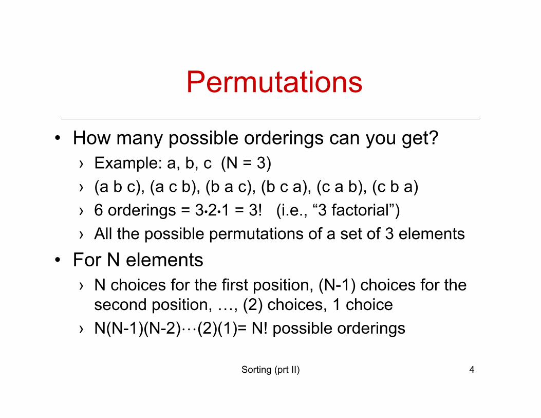
Permutations
• How many possible orderings can you get?› Example: a, b, c (N = 3)› (a b c), (a c b), (b a c), (b c a), (c a b), (c b a) › 6 orderings = 3•2•1 = 3! (i.e., “3 factorial”)› All the possible permutations of a set of 3 elements
• For N elements› N choices for the first position, (N-1) choices for the
second position, …, (2) choices, 1 choice› N(N-1)(N-2)L(2)(1)= N! possible orderings
Sorting (prt II) 5
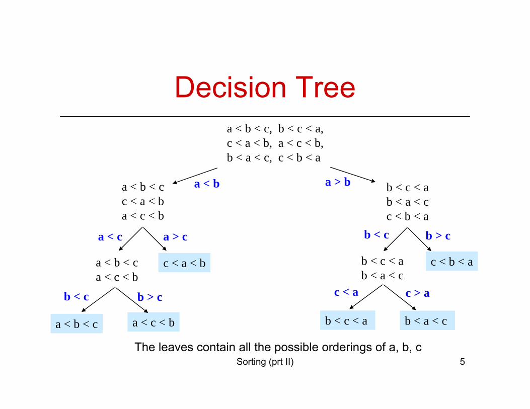
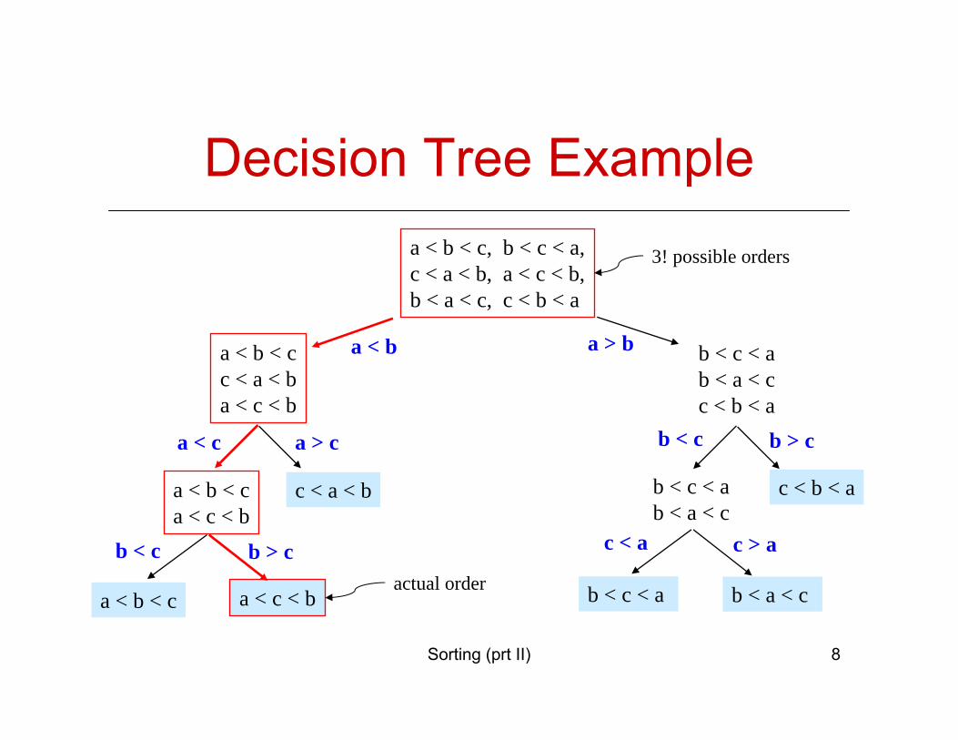
Decision Treea < b < c, b < c < a,c < a < b, a < c < b,b < a < c, c < b < a
a < b < cc < a < ba < c < b
b < c < ab < a < c c < b < a
a < b < ca < c < b
c < a < b
a < b < c a < c < b
b < c < ab < a < c
c < b < a
b < c < a b < a < c
a < b a > b
a > ca < c
b < c b > c
b < c b > c
c < a c > a
The leaves contain all the possible orderings of a, b, c
Sorting (prt II) 6
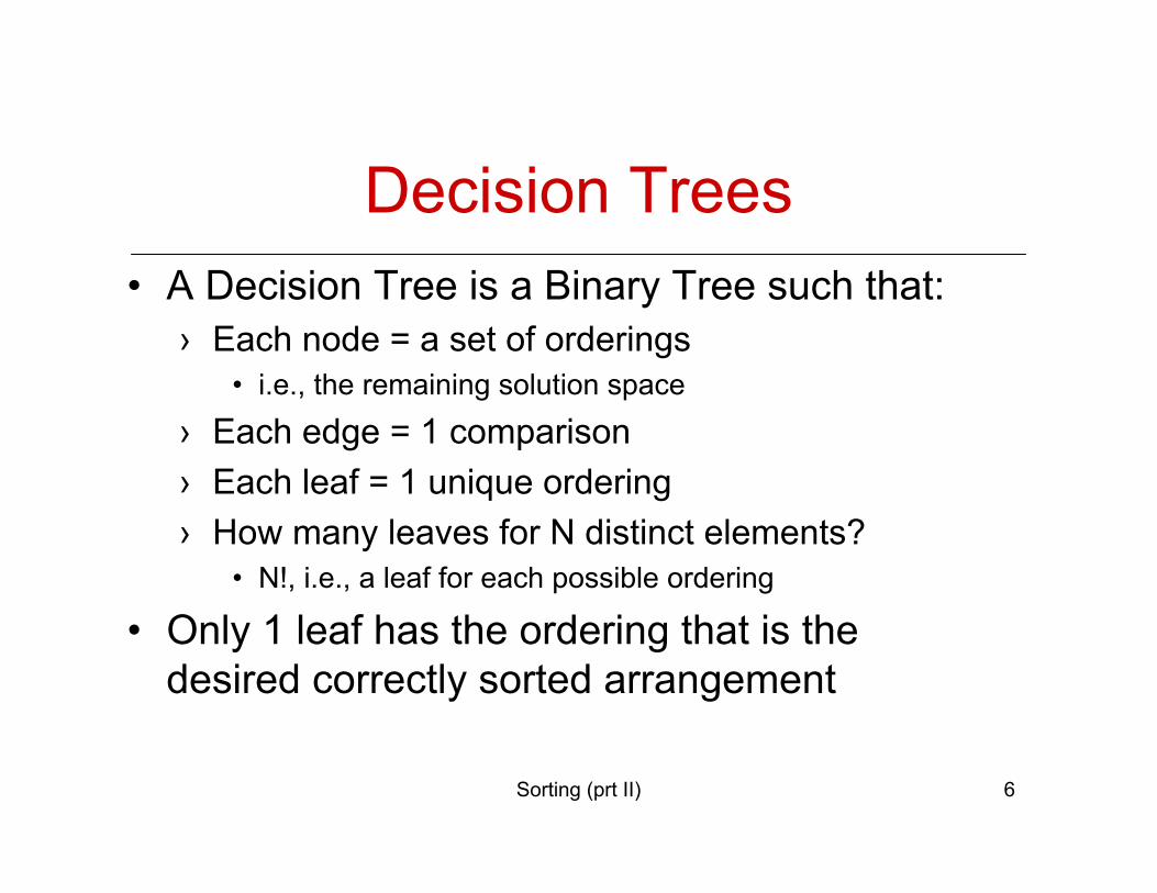
Decision Trees• A Decision Tree is a Binary Tree such that:
› Each node = a set of orderings• i.e., the remaining solution space
› Each edge = 1 comparison› Each leaf = 1 unique ordering› How many leaves for N distinct elements?
• N!, i.e., a leaf for each possible ordering
• Only 1 leaf has the ordering that is the desired correctly sorted arrangement
Sorting (prt II) 7
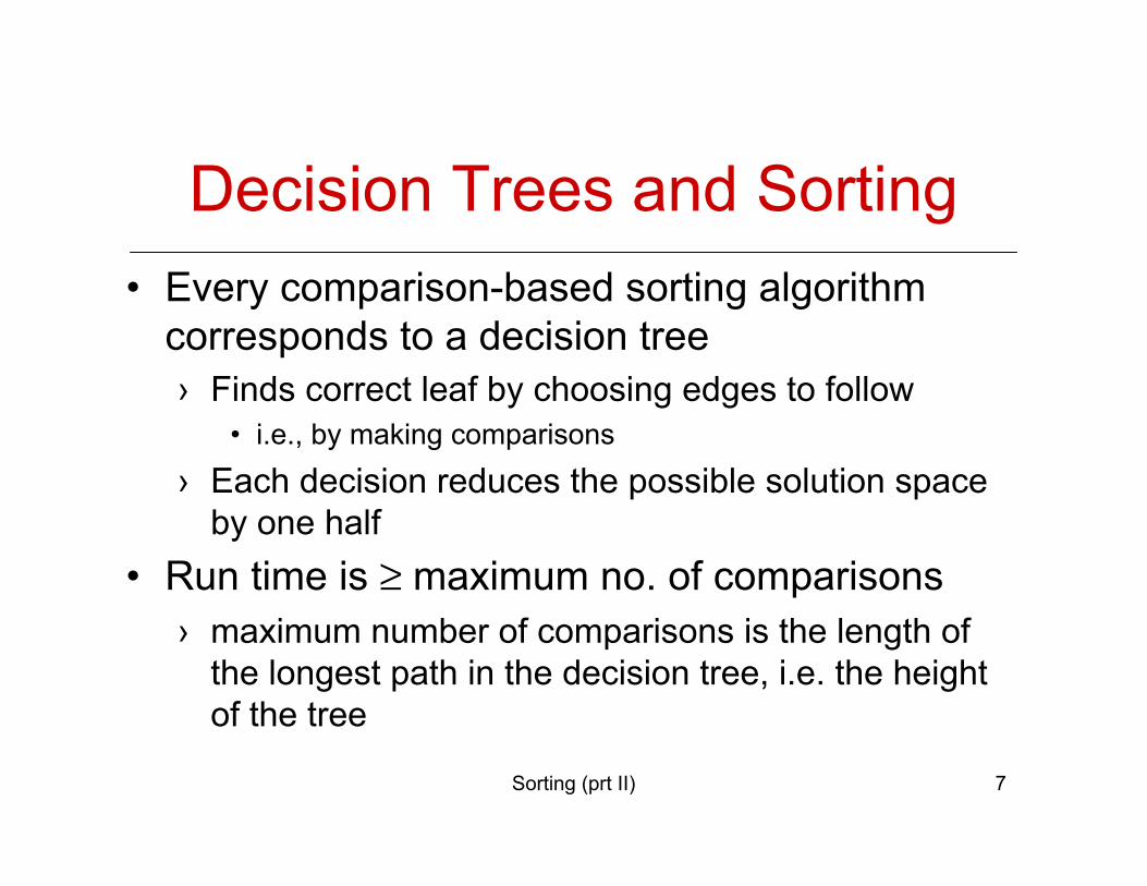
Decision Trees and Sorting• Every comparison-based sorting algorithm
corresponds to a decision tree› Finds correct leaf by choosing edges to follow
• i.e., by making comparisons
› Each decision reduces the possible solution space by one half
• Run time is ≥ maximum no. of comparisons› maximum number of comparisons is the length of
the longest path in the decision tree, i.e. the height of the tree
Sorting (prt II) 8
Decision Tree Examplea < b < c, b < c < a,c < a < b, a < c < b,b < a < c, c < b < a
a < b < cc < a < ba < c < b
b < c < ab < a < c c < b < a
a < b < ca < c < b
c < a < b
a < b < c a < c < b
b < c < ab < a < c
c < b < a
b < c < a b < a < c
a < b a > b
a > ca < c
b < c b > c
b < c b > c
c < a c > a
3! possible orders
actual order
Sorting (prt II) 9
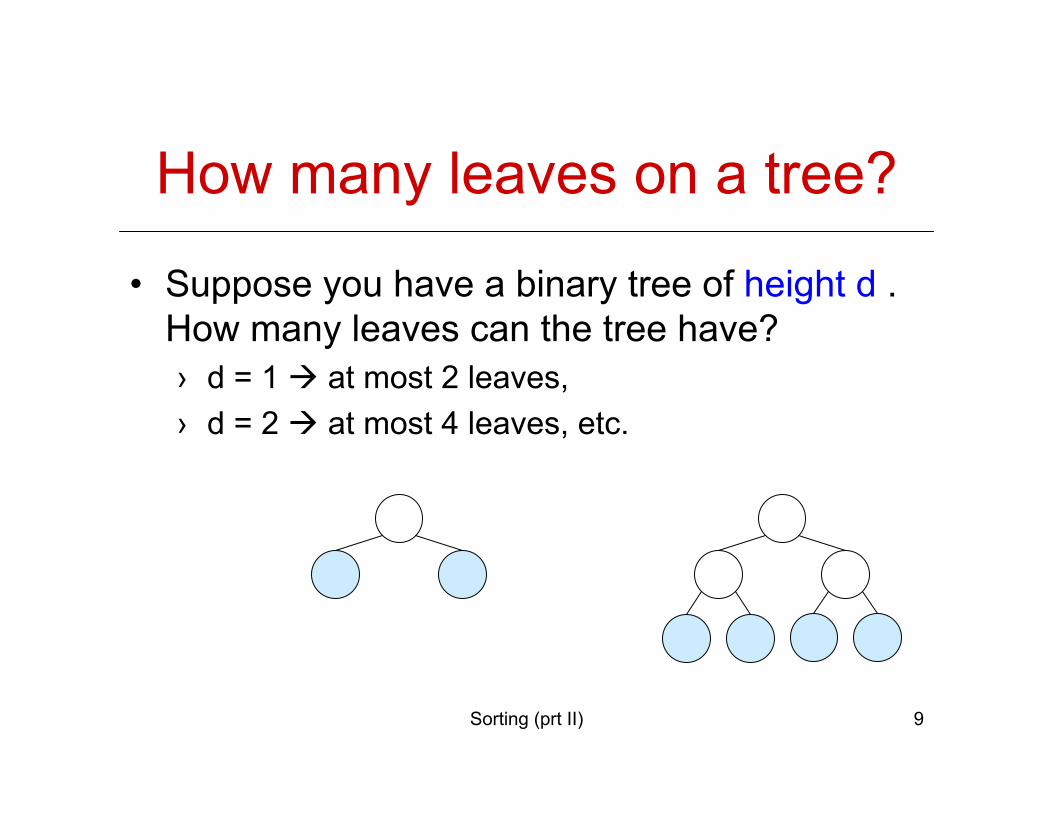
How many leaves on a tree?
• Suppose you have a binary tree of height d . How many leaves can the tree have?› d = 1 at most 2 leaves, › d = 2 at most 4 leaves, etc.
Sorting (prt II) 10
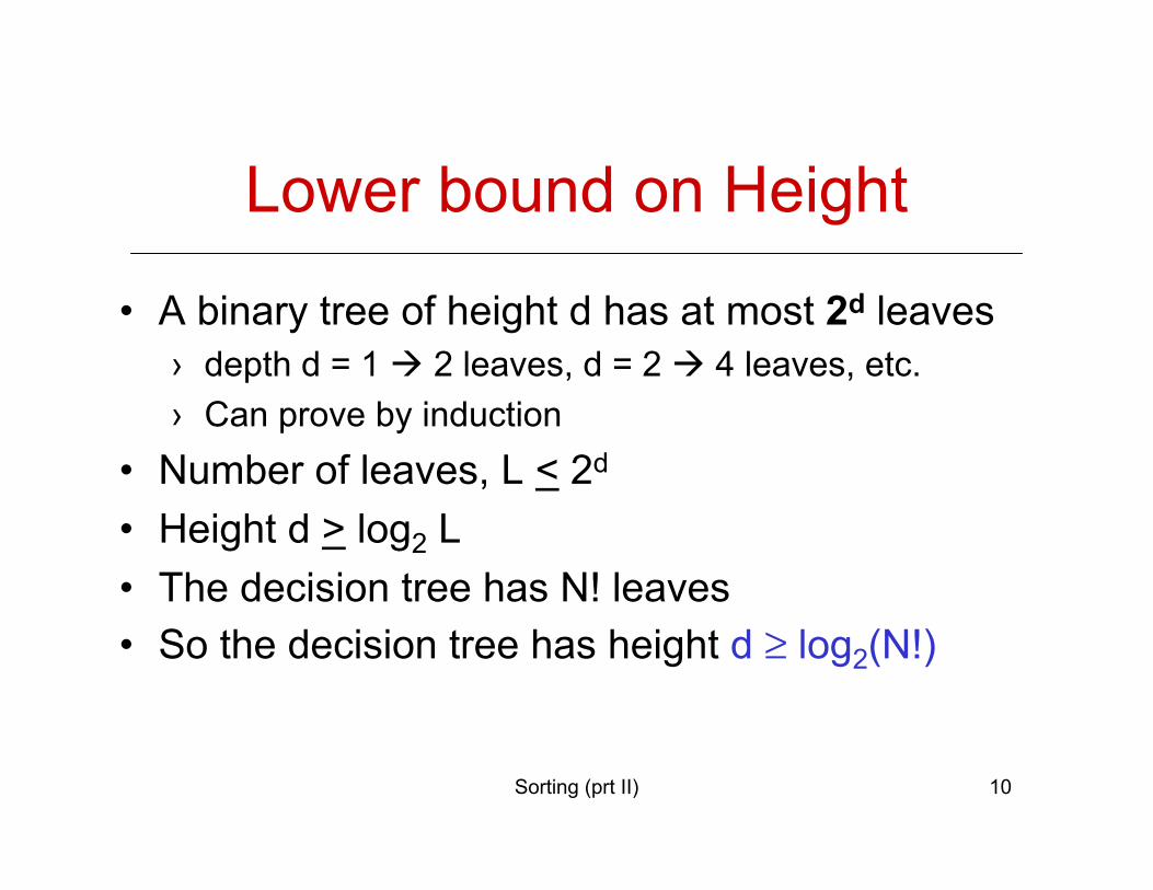
Lower bound on Height
• A binary tree of height d has at most 2d leaves› depth d = 1 2 leaves, d = 2 4 leaves, etc.› Can prove by induction
• Number of leaves, L < 2d
• Height d > log2 L • The decision tree has N! leaves• So the decision tree has height d ≥ log2(N!)
Sorting (prt II) 11
Upper Bounds and Lower Bounds
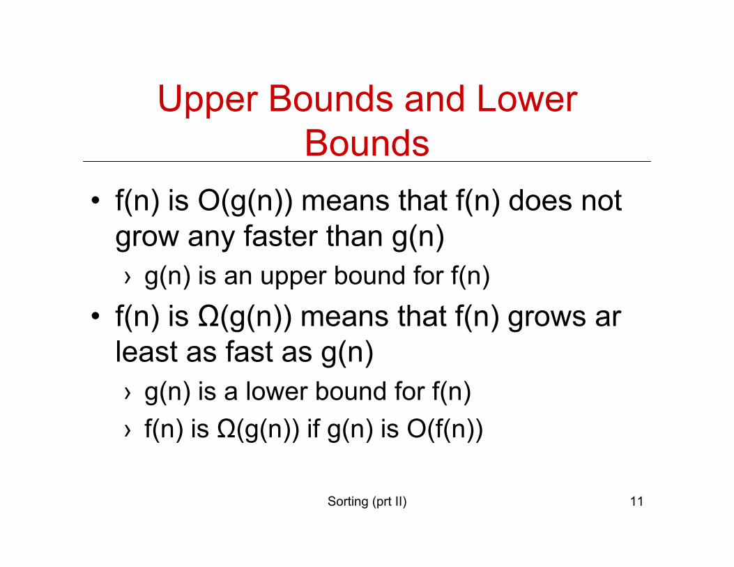
• f(n) is O(g(n)) means that f(n) does not grow any faster than g(n) › g(n) is an upper bound for f(n)
• f(n) is Ω(g(n)) means that f(n) grows arleast as fast as g(n)› g(n) is a lower bound for f(n)› f(n) is Ω(g(n)) if g(n) is O(f(n))
Sorting (prt II) 12
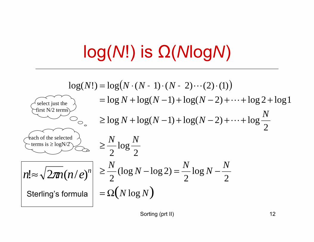
log(N!) is Ω(NlogN)
( )
)( log2
log2
)2log(log2
2log
2
2log)2log()1log(log
1log2log)2log()1log(log)1()2()2()1(log)!log(
NN
NNNNN
NN
NNNN
NNNNNNN
Ω=
−=−≥
≥
++−+−+≥
+++−+−+=⋅−⋅−⋅=
L
L
L
select just thefirst N/2 terms
each of the selectedterms is ≥ logN/2
nennn )/(2! π≈Sterling’s formula
Sorting (prt II) 13
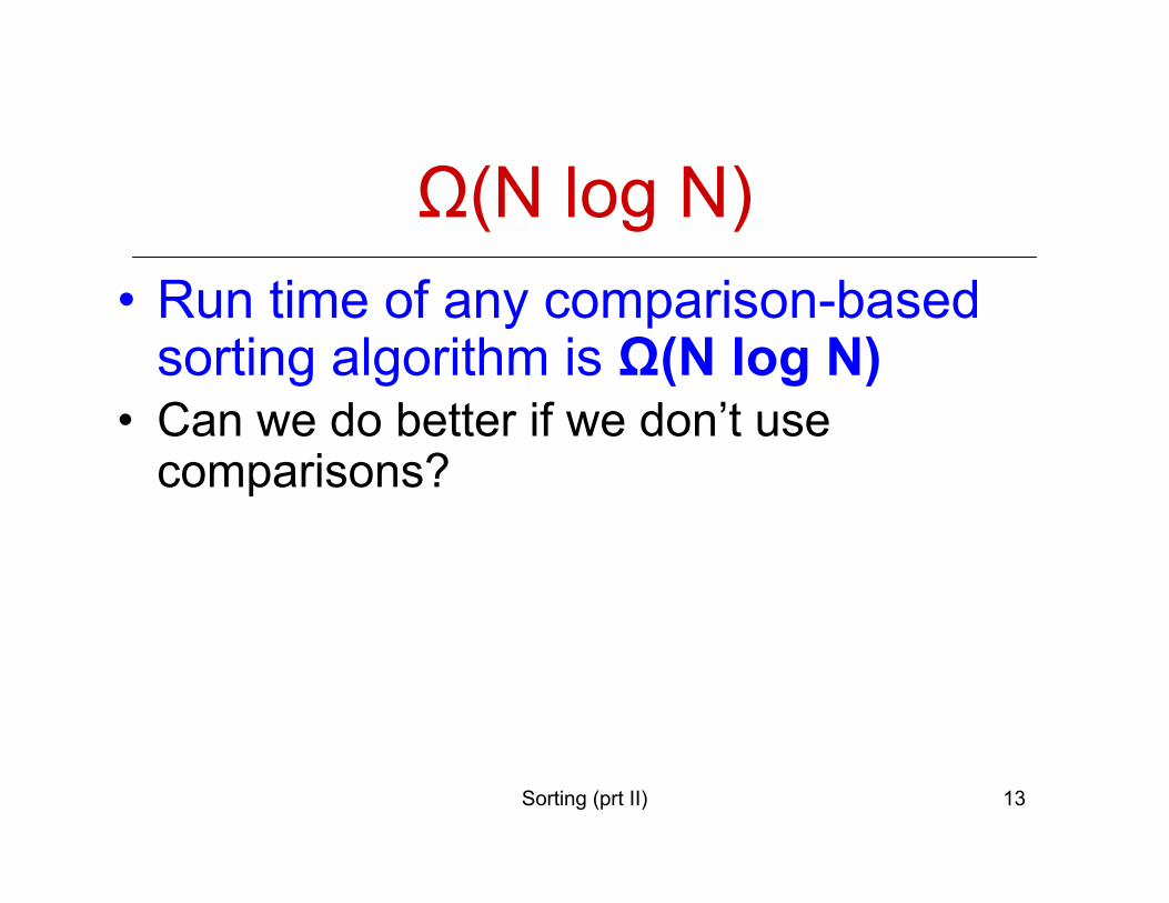
Ω(N log N)• Run time of any comparison-based
sorting algorithm is Ω(N log N) • Can we do better if we don’t use
comparisons?
Sorting (prt II) 14
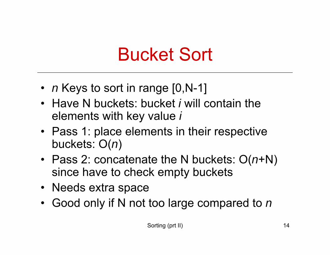
Bucket Sort
• n Keys to sort in range [0,N-1]• Have N buckets: bucket i will contain the
elements with key value i• Pass 1: place elements in their respective
buckets: O(n)• Pass 2: concatenate the N buckets: O(n+N)
since have to check empty buckets• Needs extra space • Good only if N not too large compared to n
Sorting (prt II) 15
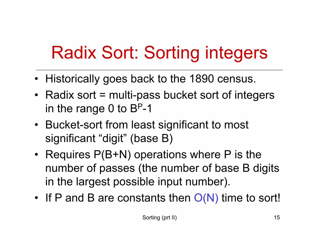
Radix Sort: Sorting integers• Historically goes back to the 1890 census.• Radix sort = multi-pass bucket sort of integers
in the range 0 to BP-1• Bucket-sort from least significant to most
significant “digit” (base B)• Requires P(B+N) operations where P is the
number of passes (the number of base B digits in the largest possible input number).
• If P and B are constants then O(N) time to sort!
Sorting (prt II) 16
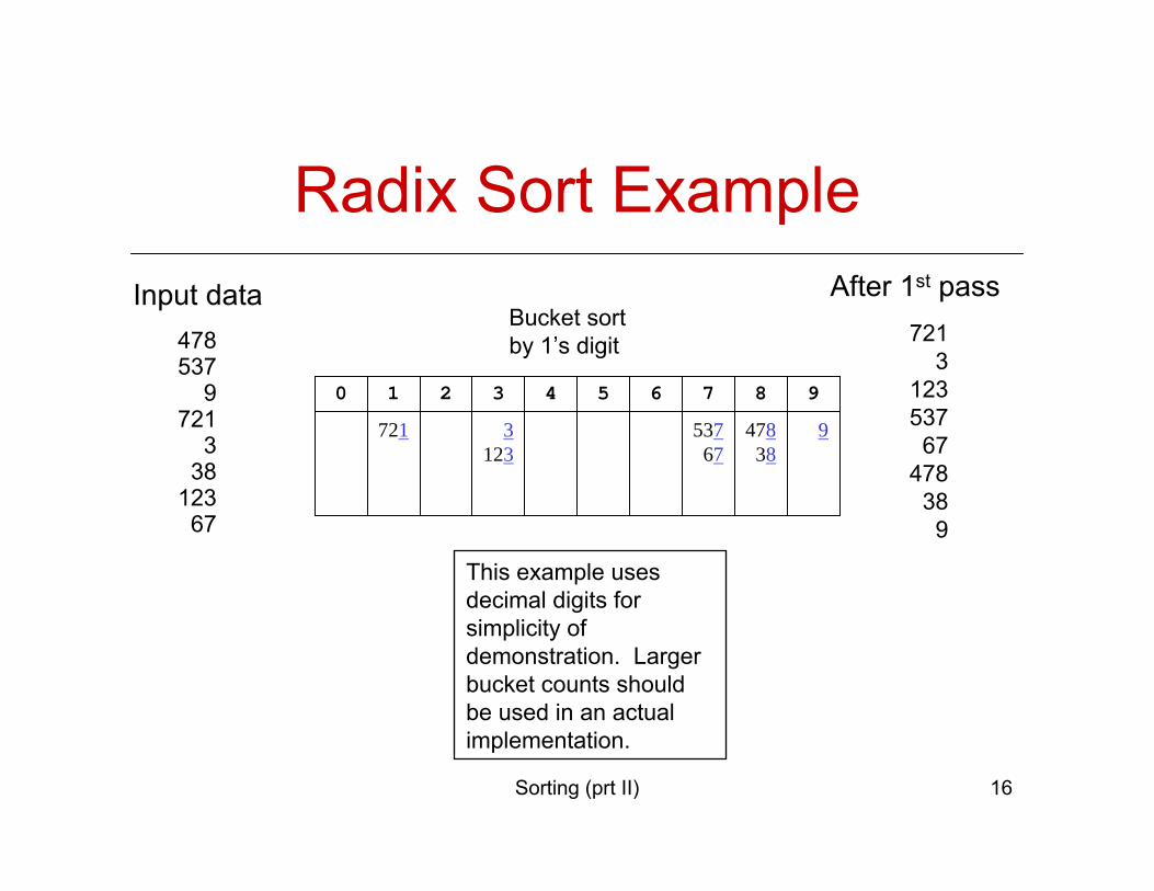
67123383
7219
537478
Bucket sort by 1’s digit
0 1
721
2 3
3123
4 5 6 7
53767
8
47838
9
9
Input data
This example uses decimal digits for simplicity of demonstration. Larger bucket counts should be used in an actual implementation.
Radix Sort Example
7213
12353767
478389
After 1st pass
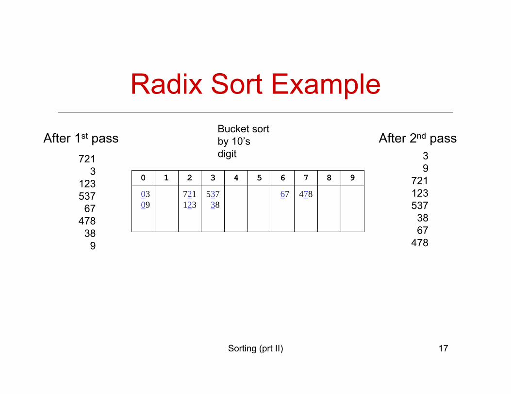
Sorting (prt II) 17
Bucket sort by 10’s digit
0
0309
1 2
721123
3
53738
4 5 6
67
7
478
8 9
Radix Sort Example
7213
12353767
478389
After 1st pass After 2nd pass39
7211235373867
478
Sorting (prt II) 18
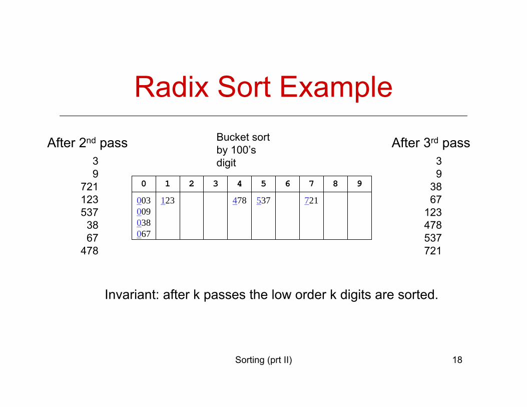
Bucket sort by 100’s digit
0
003009038067
1
123
2 3 4
478
5
537
6 7
721
8 9
Radix Sort Example
After 2nd pass39
7211235373867
478
After 3rd pass39
3867
123478537721
Invariant: after k passes the low order k digits are sorted.
Sorting (prt II) 19
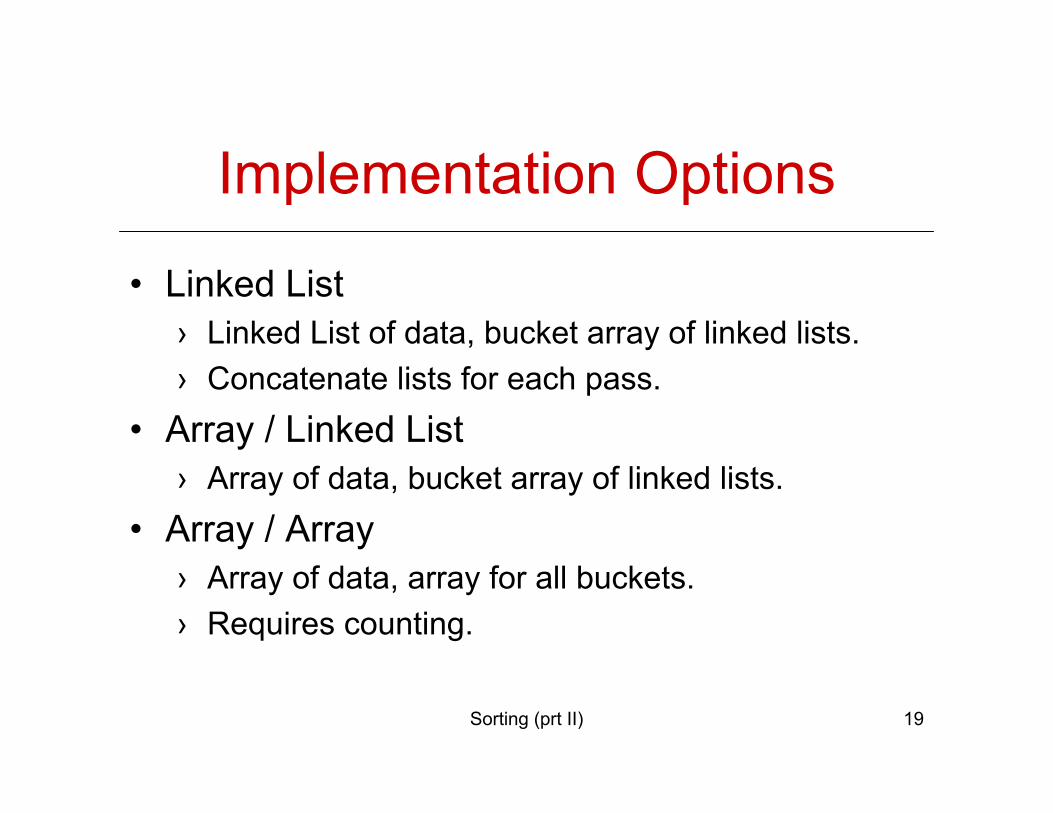
Implementation Options
• Linked List› Linked List of data, bucket array of linked lists.› Concatenate lists for each pass.
• Array / Linked List› Array of data, bucket array of linked lists.
• Array / Array› Array of data, array for all buckets.› Requires counting.
Sorting (prt II) 20
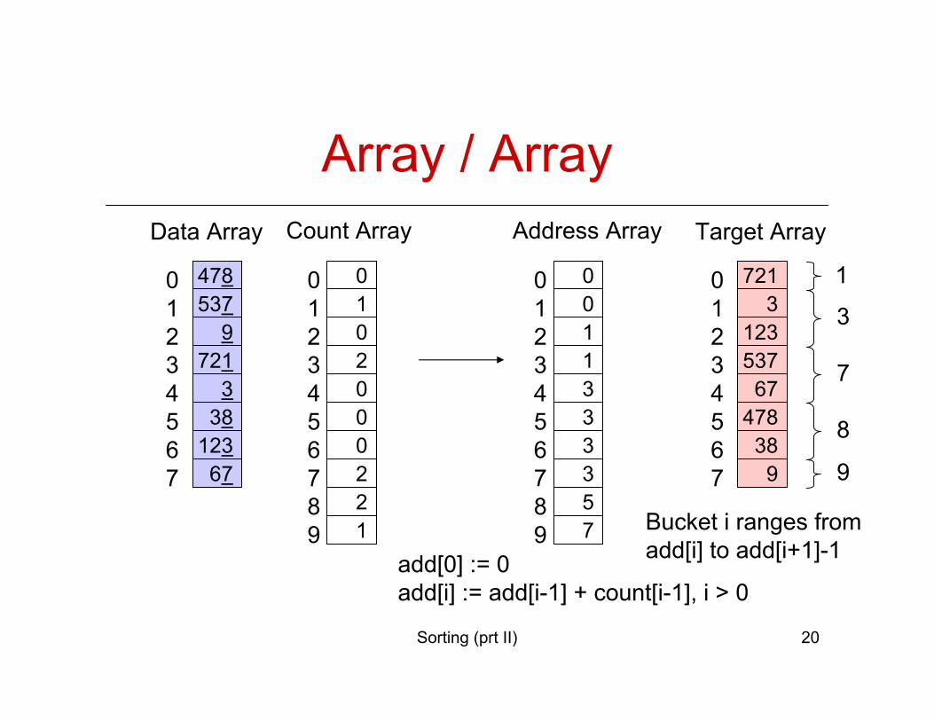
Array / Array
478537
9721
338
12367
01234567
Data Array
01020002
0123456789
21
Count Array
00113333
0123456789
57
Address Array
add[0] := 0add[i] := add[i-1] + count[i-1], i > 0
7213
12353767
47838
9
01234567
Target Array
Bucket i ranges fromadd[i] to add[i+1]-1
1
3
7
8
9
Sorting (prt II) 21
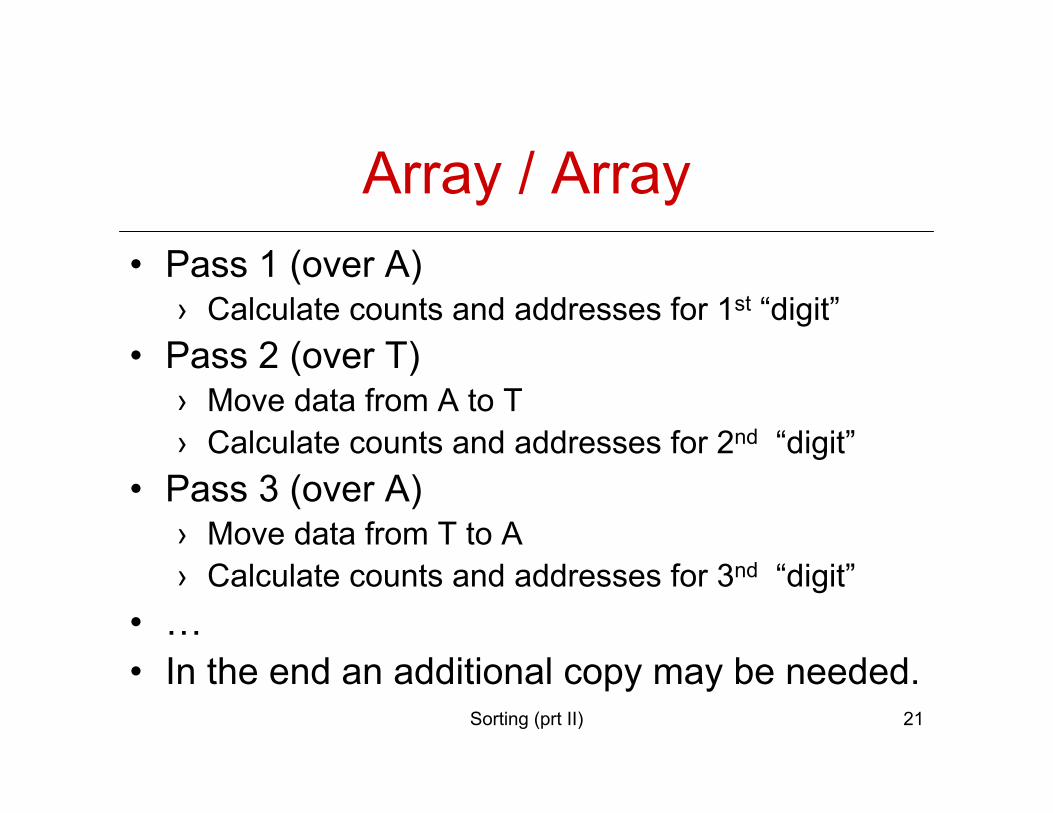
Array / Array• Pass 1 (over A)
› Calculate counts and addresses for 1st “digit”• Pass 2 (over T)
› Move data from A to T› Calculate counts and addresses for 2nd “digit”
• Pass 3 (over A)› Move data from T to A› Calculate counts and addresses for 3nd “digit”
• …• In the end an additional copy may be needed.
Sorting (prt II) 22
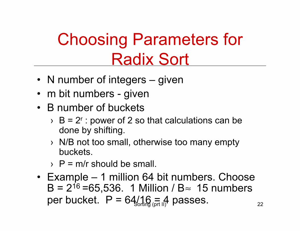
Choosing Parameters for Radix Sort
• N number of integers – given• m bit numbers - given• B number of buckets
› B = 2r : power of 2 so that calculations can be done by shifting.
› N/B not too small, otherwise too many empty buckets.
› P = m/r should be small.• Example – 1 million 64 bit numbers. Choose
B = 216 =65,536. 1 Million / B ≈ 15 numbers per bucket. P = 64/16 = 4 passes.
Sorting (prt II) 23
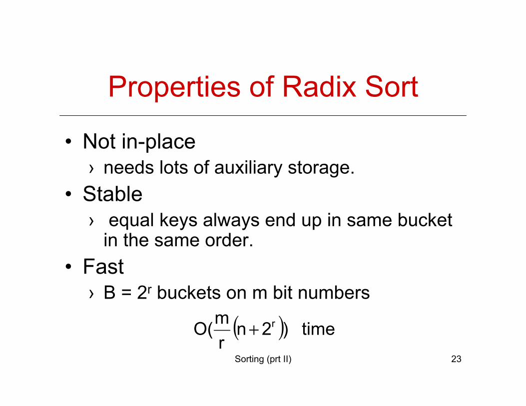
Properties of Radix Sort
• Not in-place › needs lots of auxiliary storage.
• Stable› equal keys always end up in same bucket
in the same order.• Fast
› B = 2r buckets on m bit numbers
( ) time )2nrmO( r+
Sorting (prt II) 24
Internal versus External Sorting
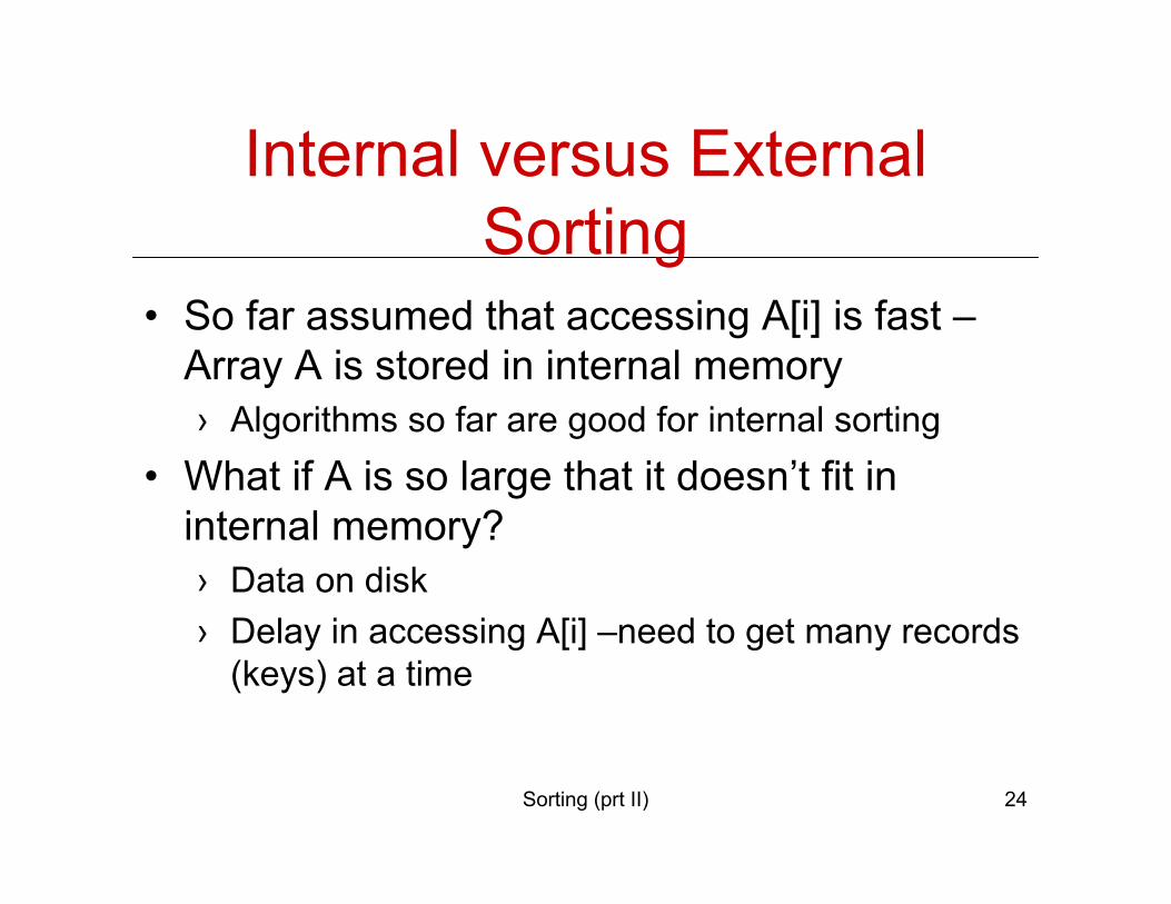
• So far assumed that accessing A[i] is fast –Array A is stored in internal memory› Algorithms so far are good for internal sorting
• What if A is so large that it doesn’t fit in internal memory?› Data on disk› Delay in accessing A[i] –need to get many records
(keys) at a time
Sorting (prt II) 25
Internal versus External Sorting
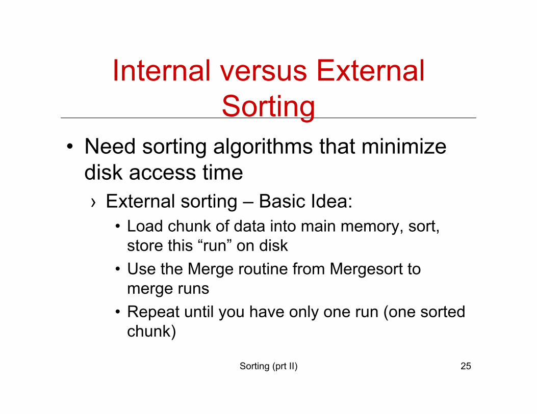
• Need sorting algorithms that minimize disk access time› External sorting – Basic Idea:
• Load chunk of data into main memory, sort, store this “run” on disk
• Use the Merge routine from Mergesort to merge runs
• Repeat until you have only one run (one sorted chunk)
Sorting (prt II) 26
Summary of Sorting
• Sorting choices:› O(N2) – Insertion Sort › O(N log N) average case running time:
• Heapsort: In-place, not stable.• Mergesort: O(N) extra space, stable.• Quicksort: claimed fastest in practice but, O(N2) worst
case. Needs extra storage for recursion. Not stable.
› O(N) – Radix Sort: fast and stable. Not comparison based. Not in-place.
Recommended