Proceedings of 8th
Windsor Conference: Counting the Cost of Comfort in a changing
world Cumberland Lodge, Windsor, UK, 10-13 April 2014. London: Network for
Comfort and Energy Use in Buildings, http://nceub.org.uk
Solving the Black Box: Inverse Approach for Ideal Building Dynamic
Behaviour Using Multi-Objective Optimization with Energyplus
Nelly Adriana Martinez
University College London, Bartlett School of Graduate Studies, Faculty of the Built
Environment, London, UK, [email protected]
Abstract
The need for zero carbon buildings is changing the trial-and-error process that Architectural design has
traditionally employed towards a system that allows wider analysis capacity at the conceptual stage. By
visualizing design as a “Black Box” where the composition variable B can be cleared from knowing the
stimuli S and the desired response R; optimal solutions arise to the surface. The Dutch FACET project
which initiated to find the ideal dynamic properties of a building shell to get the desired indoor climate at variable outdoor conditions implemented this inverse approach and served as inspiration for this
work which will build on their findings but implementing a two-step methodology. (1) Fabric
properties where optimized using EnergyPlus+jEPlus+EA aiming to reduce heating & cooling energy
and minimize thermal and visual discomfort. (2) Best solutions were used to create an ideal dynamic
building using the best performance at each timestep and interchanging material properties accordingly.
The results presented indicate that adaptive behaviour stands as a promising way to harmonize energy
consumption and discomfort levels conflictive nature.
Keywords: Multi-objective optimization, Dynamic building, EnergyPlus, jEPlus+EA
1. Introduction
The ever changing conditions that a building is subject to, make reaching optimal
performance along the entire time a difficult task to achieve. Weather and user
patterns greatly fluctuate along time in contrast to the steady parameters that are
perceived as comfortable for the people inside them. They are the bases that
determine energy consumption for, whenever these are not meet, artificial systems
enter to recreate a benevolent atmosphere. This contradictory paradigm along with the
traditional way of conceiving buildings as static elements places their design out of
context; not following the logic behind a dynamic environment.
The search for a built environment that reconciles energy efficiency, comfort and
health has led to strategies that follow passive and nature design concepts, artificial
systems efficiency or alternative energy sources. Although these paths have for sure
signified a progress; current building stock performance shows that much is still left
to do. Proposing buildings with the capacity to mutate offers the possibility to
combine the best of these strategies and provide optimal performance under any
circumstance.
Acting as the difference between the exterior and interior; adaptations of the building
fabric have the greatest potential to transform conditions into acceptable ranges by
changing its properties and by hence the way energy is balanced. Advances in
technology and material science have made this a possibility already achievable; a
series of “smart windows” can vary opacity or infrared transmittance according to
different conditions and Nanotechnology and Micro-engineering have found in the
atomic level a way to manufacture materials that respond in ways that were not
possible before.
Incorporation of adaptive behaviour is changing the Architectural method from
solving a space to solving a process (Loonen 2010), where successful designs are
determined by the analysis capacity at the conceptual stage when the world of
possibilities is large. This work will explore the implications that adaptive behaviour
in buildings carry to the design conception and emerging tools identified by previous
research in the field (Wang et al. 2005), (Bakker et al. 2009), such as Multi-objective
Optimization (MOO) and the Inverse Approach for their potential to balance the
conflict between comfort and energy savings.
2. Building Adaptive Concepts
Multiple adjectives are commonly used in an attempt to describe a building’s non-
static behaviour. Such buildings are commonly referred in literature as: active,
dynamic, adaptive, kinetic, responsive, living, smart, interactive, high performance or
advanced, to name some (Schnadelback 2010), (Loonen et al. 2013), (Velikov &
Thün 2013). Since few years ago different initiatives have tried to cluster and define
under one concept these buildings that accommodate to the ever changing external
and internal conditions in a search for communication, energy efficiency, health and
comfort.
Environmentally Responsive
The Energy Conservation in Buildings & Community Systems (ECBCS) programme,
coordinated by the International Energy Agency (IEA) In 2004, unified the concept
under Responsive Building Concepts (RBC) & Responsive Building Elements (RBE)
which definition and design guidelines were published in Annex 44 (Aschehoug &
Perino 2009), (Heiselberg 2012). In this case responsive referred to the ability for
energy capture, energy transport and/or energy storage (Heiselberg 2009). Information
from existing cases was collected in an aim to maximize their potential and a design
approach which articulated responsive building elements, building services and
renewable energy systems through an integrated design process where the different
experts are involved from the conceptual stage was proposed. Its weakness is that they
relied on the same method architecture had been conceived and focused only on
commercial technologies.
Adaptive Architecture
This concept stills somewhat ambiguous but seems to have begun to form about a
decade ago in an effort to describe these emerging examples. Its objectives are not
only environmental but also societal and communicational. Even though many authors
have discussed it; perhaps the best effort to give it a framework are those by
(Lelieveld et al. 2007) who as part of her Ph.D. defined it as “Architecture from which
specific components can be changed in response to external stimuli” and
(Schnadelback 2010) who defined its drivers, what they react to, methods, elements
and effects. Although his categorization has a humanistic approach where
environmental goals belong to the social motivations together with lifestyle and
fashion; it allows inclusion of internal and aesthetic adaptations regardless of whether
or not they have a physical effect.

Climate Adaptive Building Shells (CABS)
Initiated in The Netherlands, hub for research in the field for several years, CABS
started as a research project between the Organization for Applied Scientific Research
(TNO), Energy Research Centre of the Netherlands (ECN) & University of Plymouth
in 2008. It was defined and contextualize by (Loonen 2010) in his MSc Thesis as:
“A climate adaptive building shell has the ability to repeatedly and reversibly change
its functions, features or behaviour over time in response to changing performance
requirements and variable boundary conditions. By doing this, the building shell
effectively seeks to improve overall building performance in terms of primary energy
consumption while maintaining acceptable thermal and visual comfort conditions.”
It is until now the best one documented with a database of around 200 built, prototype
and patented cases (Loonen n.d.). His categorization was found to be the most
successful as it uses simulation tools logic, layering them according to the physical
domain involved and presenting them as the result of a process. It will be the one on
which sections 2.1 and 2.2 develop.
2.1. Adaptation Mechanisms
Adaptation in architecture has been found to be determined by either the material’s
inherent ability to change (micro-scale) or a mechanism assembled to produce the
transformation (macro-scale). At the micro-scale, physical properties of materials vary
according to how they convert a certain energy input (potential, electrical, thermal,
mechanical, chemical, nuclear and kinetic). When this energy affects the material’s
molecular structure the result is a change of its properties, but when it is the energy
state the one affected then the result is an exchange of energy. In one, the energy is
absorbed and the material undergoes a transformation while in the other the material
stays the same but the energy changes (Addington & Schodek 2005). At the macro-
scale properties are changed through movable parts using the effect of forces for
moving objects and involving the dimension of time (Crespo 2007). They operate
according to ambient, scheduled or personal preferences and changes are triggered by
a sensor that registers conditions and drives the data to be interpreted by a processor
which subsequently sends a signal to the corresponding actuator for an action to be
executed.
Whatever the adaptive mechanism is, it requires a time lag to change from one state to
another which could happen from a matter of seconds to hours, days, seasons and so
on. Moreover the mechanism driving the change not always performs the same on
both directions, for example reactions activated through chemical means can return to
the original state thermally or materials that obscure according to temperature perform
differently when heating up than when cooling down; quality known as Hysteresis.
2.2. Physical Domains
In the realm of controlling external varying conditions to keep an ideal internal
environment; skin has given the example to follow being object of multiple analogies
in architecture (Vassela 1983), (Drake 2007). Human skin adapts to temperature and
humidity, is waterproofed but permeable to moisture, feels draft and touch and repairs
itself keeping organs healthy and comfortable (Wigginton & Harris 2002). Being the
limit between outdoors and indoors, just as skin, the building envelope is exposed to a
diversity of forces and therefore has the ability to regulate them as required. Loonen

distinguished four physical domains with their respective interdependencies on which
CABS act in order to adjust internal conditions: Thermal, Optical, Air-flow and
Electrical (See Figure 1) and suggested Sound and Moisture as possibilities not
included for not existing yet an example (Loonen et al. 2013).
Figure 1. CABS Physical Domains
This categorization simplified the complexity embed in building adaptation but mixed
an end-result with the means to achieve it. In terms of energy efficiency, Optical
properties of materials can be adjusted to improve thermal comfort but adaptations
that just end up in a change of visual perception are not relevant. The same case
applies to the Electrical and Air-flow domains; adaptations that generate electricity
are only relevant if it is actually used to improve building’s performance and the Air-
flow ones only if they act on indoor air quality and thermal comfort. More over the
scope should allow space for all the required needs regardless of whether or not
examples exist, although materials that absorb moisture (Hygroscopic) have been
known for years and research shows they can moderate indoor humidity conditions
(Simonson et al. 2004). Products like hydrogel are being investigated to
absorb/release air water vapour to control indoor humidity (Johnson & Kulesza 2007).
Researches like “Building Things that Talk II” by the Responsive Skins Initiative
(Yazdani et al. 2011) shows how an acoustic stimuli could trigger an actuator which
could easily be translated into buildings that can control the decibel levels admitted.

To overcome these limitations a new scheme is proposed identifying five domains that adaptations
targeting to reduce energy consumption and maximize comfort pursue (See
Figure 2): Thermal, Visual, Moisture, Acoustic and Indoor Air Quality (IAQ), where
each one is achievable through four different means or their interrelation: Electrical,
Optical, Mechanical or by Reaction (Chemical, Radiant, Magnetic, Thermal, Fluid).
Even though adaptation in buildings might have other targets such as communication
or social connectivity those have not been explored in this work.
Figure 2. Adaptation Target Scheme
T – Thermal
M – Moisture
A – Acoustic
I – Indoor Air Quality
V – Visual
3. Solving the Black Box
A black box is an imaginary representation of a set of systems affected by a stimuli S
and out of which reactions R emerge. The constitution and structure of the box are
irrelevant and only the behaviour of the system matters. This is what one of the
greatest second order cyberneticians referred to as “trivial machine”; one which
couples a particular stimulus with a specific response (Foerster 2003). In his work he
mentions that all machines we construct or buy are, hopefully, of this kind to perform
the task they have been designed for.
Our search for buildings that do not require fossil fuels inevitably leads to the
investigation of unusual devises (Glynn 2008); where cybernetics has several lessons
for building designers as adaptive systems are intrinsically dynamic becoming the
design of a process rather than an “artefact” (Moloney 2007).
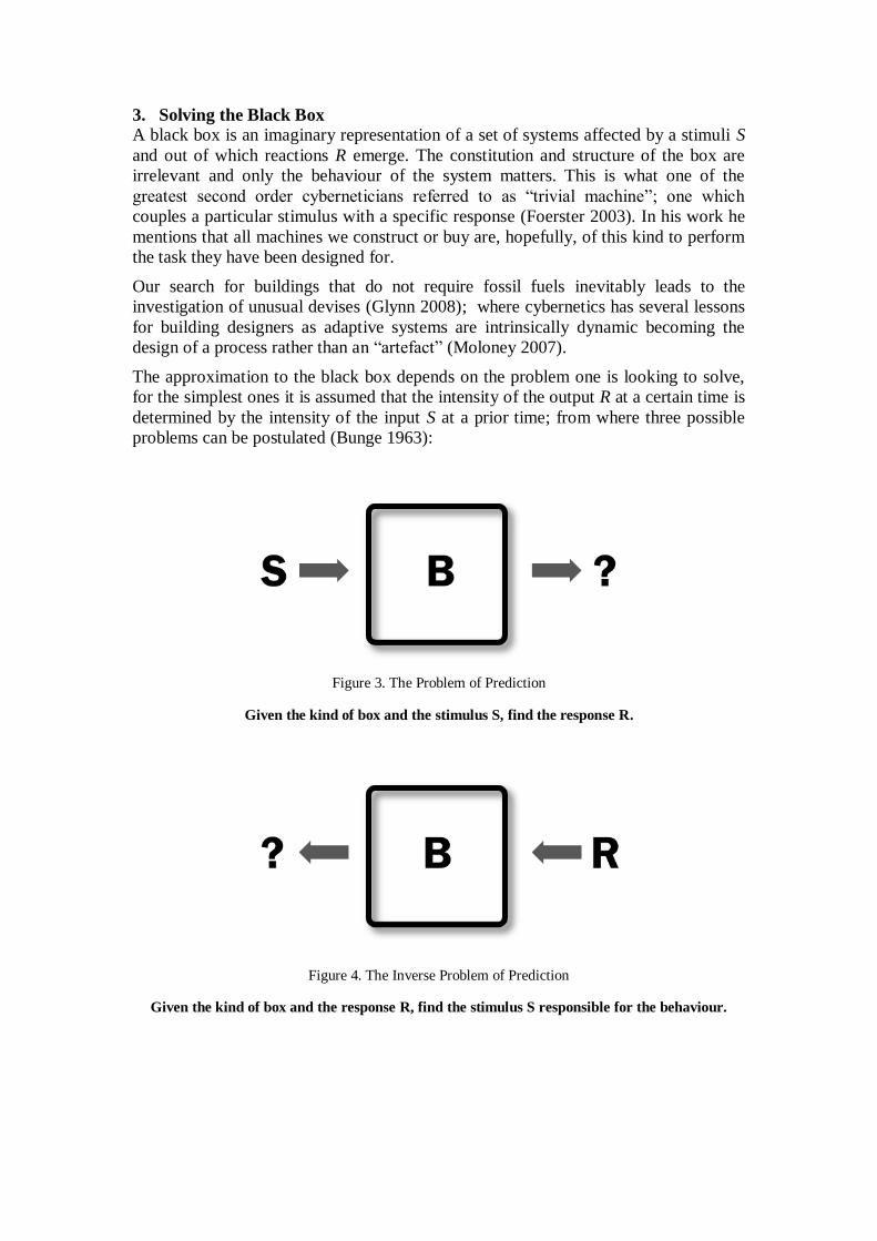
The approximation to the black box depends on the problem one is looking to solve,
for the simplest ones it is assumed that the intensity of the output R at a certain time is
determined by the intensity of the input S at a prior time; from where three possible
problems can be postulated (Bunge 1963):
Figure 3. The Problem of Prediction
Given the kind of box and the stimulus S, find the response R.
Figure 4. The Inverse Problem of Prediction
Given the kind of box and the response R, find the stimulus S responsible for the behaviour.

Figure 5. The problem of explanation
Given the behaviour R under a known stimuli S, find the kind of box that accounts for the
behaviour.
In the case of buildings the problem might not be as “obscure” and could be better
addressed as “Gray Box” due to the fact that they have enough internal constrains
based on physical laws built into them (Reddy 1989). Architectural design has been
treated as the kind of problem number 1 where once a design is proposed; its
performance is calculated hoping to get the desired results. No wonder why we have
failed in the design of a simple trivial machine and our buildings don’t behave the
way we want.
Five years ago the Dutch FACET project was initiated with the objective to solve the
question of: “What would be the ideal, dynamic properties of a building shell to get
the desired indoor climate at variable outdoor climate conditions?” (de Boer n.d.);
which has been the inspiration for the present work. This query specifically deals with
the kind of problem number 3 and, as Bunge describes, is not well-determined and
therefore does not have a unique solution.
3.1. Methodology
An ideal building would provide comfort with zero energy implications, dynamic
adaptations of the fabric could absorb the ever changing external climate to keep
internal conditions in the narrow comfort band with the lowest energy use. This work
has focused on thermal and visual conditions as comfort indicators and cooling and
heating loads as the energy ones. The desired thermal comfort will be based on
ASHRAE 55-2004 humidity ratio and operative temperature parameters using a Clo
level of 0.5 for summer and 1.0 for winter. While optimal visual comfort will be
based on a maximum allowable discomfort glare index of 22 as recommended in
(EnergyPlus 2013b) reference guide.
To find the parameters that a fabric should have in order to obtain the desired
indicators a method called “System Parameter Identification” colloquially referred to
as the “Inverse Approach” will be implemented. It is commonly applied to existing
buildings as it is a technique where energy behaviour is identified from performance
records while in actual operation (Reddy 1989). Input data typically includes static
building information and dynamic (time dependent) weather and energy consumption
reports (An et al. 2012). This time building information will be dynamic and energy
consumption and discomfort static at zero (or to approximate zero) replacing thus
metered reports and enabling the method to be used at a design phase.

The FACET project proposed the inverse approach as a feasible way to find ideal
properties of adaptive shells (Boer et al. 2011), (Boer et al. 2012), (Bakker et al. 2009)
but, while it was running, only got to evaluate comfort and energy independently and
analysed adaptivity simply in terms of what smart façade glazing and adjustable
shading options could offer disregarding opaque surfaces potential. It also proposed
the implementation of multi-objective optimization (MOO) as a future step to
visualize the performance benefits of CABS going beyond what static designs could
offer towards a utopia point where comfort and energy don’t conflict (Boer et al. 2011)
(See Figure 6).
Figure 6. CABS Improved Pareto Set (Boer et al. 2011)
This paper will built on their work but simultaneously consider both; visual and
thermal comfort in association with building energy consumption while MOO will be
used to evaluate those fabric variables that would offer optimal results to be the base
on which an ideal dynamic building will be built. Two steps have been implemented
in the process; first, different material properties will be optimised with three
objectives in mind: reduce heating & cooling energy and minimize thermal and visual
discomfort. Second, the best solutions from optimization results will be used to create
an ideal dynamic behaviour by finding the best performance at each timestep of one
hour and interchanging material properties accordingly. Chapter 4 (step 1) and
Chapter 5 (step 2) will describe the particular methodology used to develop each step
and their findings.
3.2. Model Description
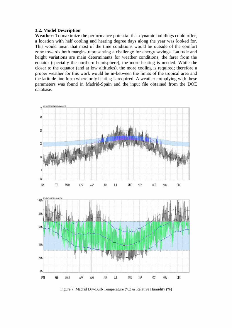
Weather: To maximize the performance potential that dynamic buildings could offer,
a location with half cooling and heating degree days along the year was looked for.
This would mean that most of the time conditions would be outside of the comfort
zone towards both margins representing a challenge for energy savings. Latitude and
height variations are main determinants for weather conditions; the farer from the
equator (specially the northern hemisphere), the more heating is needed. While the
closer to the equator (and at low altitudes), the more cooling is required; therefore a
proper weather for this work would be in-between the limits of the tropical area and
the latitude line form where only heating is required. A weather complying with these
parameters was found in Madrid-Spain and the input file obtained from the DOE
database.
Figure 7. Madrid Dry-Bulb Temperature (°C) & Relative Humidity (%)
Geometry: A simple one zone building was built in EnergyPlus 8 m in length, 6 m
wide and 2.7 m height (Area = 48 m Volume = 129.6) with walls oriented
perpendicular to each cardinal direction. Due to its northern location an opening was
placed at the south maximizing passive solar heat gains in winter. Glazing ratio was
kept at 50% with window dimensions of 5.4 m in length and 2 m height starting at
0.35 m above floor level. It is an open plan office for two people with walls and roof
exposed to the external environment and no external shading from devices, vegetation
or other buildings which could benefit internal conditions for results to show the
effects of the fabric itself.
Construction: Glazing and building fabric were built in one layer setting their
properties as a variable which could be substituted with values from a specified range
according MOO criteria. This was done using jEPlus (Zhang et al. 2011) the
parametric tool for EnergyPlus designed to test different model parameters
simultaneously. The tool generates commands for EnergyPlus to run and collects the
results afterwards. Even though the parametric pre-processor utility has been included
in EnergyPlus since recent versions, not requiring coupling it to an external tool
anymore; this method was used as the MOO software applied is designed to handle
the process through jEPlus.
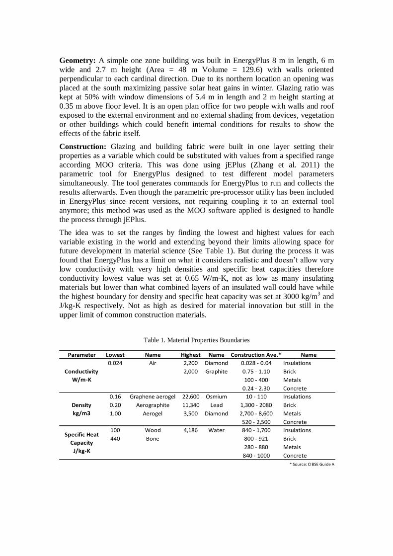
The idea was to set the ranges by finding the lowest and highest values for each
variable existing in the world and extending beyond their limits allowing space for
future development in material science (See Table 1). But during the process it was
found that EnergyPlus has a limit on what it considers realistic and doesn’t allow very
low conductivity with very high densities and specific heat capacities therefore
conductivity lowest value was set at 0.65 W/m-K, not as low as many insulating
materials but lower than what combined layers of an insulated wall could have while
the highest boundary for density and specific heat capacity was set at 3000 kg/m3 and
J/kg-K respectively. Not as high as desired for material innovation but still in the
upper limit of common construction materials.
Table 1. Material Properties Boundaries
Parameter Lowest Name Highest Name Construction Ave.* Name
0.024 Air 2,200 Diamond 0.028 - 0.04 Insulations
2,000 Graphite 0.75 - 1.10 Brick
100 - 400 Metals
0.24 - 2.30 Concrete
0.16 Graphene aerogel 22,600 Osmium 10 - 110 Insulations
0.20 Aerographite 11,340 Lead 1,300 - 2080 Brick
1.00 Aerogel 3,500 Diamond 2,700 - 8,600 Metals
520 - 2,500 Concrete
100 Wood 4,186 Water 840 - 1,700 Insulations
440 Bone 800 - 921 Brick
280 - 880 Metals
840 - 1000 Concrete
Density
kg/m3
Conductivity
W/m-K
Specific Heat
Capacity
J/kg-K
* Source: CIBSE Guide A

Thicknesses were set fixed using widths common in construction practices (Walls =
0.5, Roof = 0.25, Floor = 0.6 m) leaving the calculated U-value and energy balance to
rely entirely on the inherent properties of the material, Table 2 summarizes material
input values. For glazing the simplified system in EnergyPlus was used setting U-
Factor range in 1 – 6.8 and the SHGC in 0.06 – 0.84.
Table 2. Material Variables Parameters
Parameter Units Walls Roof Floor
Thickness m 0.50 0.25 0.6
Conductivity W/m-K
Density kg/m3
Specific Heat Capacity J/kg-K
Thermal Absorptance
Solar Absorptance 0.7 0.7 0.7
Visible Absorptance 0.7 0.7 0.7
* Values not as low or high due to software limitations
0.65* - 3000
0.1 - 3000*
100 - 3000*
0.1 - 0.9
Internal Conditions: The zone worked as a mixed mode system where natural
ventilation is allowed through windows when indoor dry bulb temperature is above
22 °C but only if the outside temperature is at least 2 °C cooler than indoor conditions.
Windows would close if wind speed is above 40 m/s when users normally would shut
them to avoid papers to blow up. Mechanical cooling or heating was set to start
whenever temperature falls outside 19 to 28 °C. The difference between the
thermostat deadband and ASHRAE 55 parameters would be classified as thermal
discomfort, even though the range would be acceptable for natural ventilation cases,
the challenge is for dynamic buildings to reach the most stringent conditions.
As standard offices the building is fully occupied only on weekdays from 8:00 to
17:00 and partially occupied from 12:00 to 14:00 and one hour before and after
working hours, simulating conditions were not everybody lunch at the same time and
where a person arrives early or leaves late. Same wise equipment was set to work
according to this schedule; the HVAC system operates only on weekdays from 5:00 to
20:00 while lighting operates 50% when there is partial occupation except for lunch
time where it keeps operating at 100%. Infiltration flow rate was estimated in 0.5
ACH and internal heat gains according to Table 3.
Table 3.Internal Conditions
People Lighting Equipment People Other
Offices 24 5.6 10 15 30% 43% -
* Source: CIBSE Guide A
Fraction
Radiant
Latent W/m2Sensible W/m2Density
person/m2Bulding Type
4. Multi-Objective Optimization
Designers often use building energy simulations on a scenario by scenario basis; first
a solution is proposed, then evaluated and subsequently a new solution is created
based on results. This iterative trial-and-error process is time consuming, ineffective
and limited as only few scenarios are able to be explored so the best solution is hardly
accomplished. One approach that assesses multiple scenarios is parametric study
where the effect of selected design variables is explored by testing some options or all
possible solutions. Despite its potential it requires long computing time and high
storage capacity (Naboni et al. 2013), not to mention the brute-force necessary to
analyse vast amount of results. The other approach is to reduce the number of
simulations by implementing the same logic nature has used to evolve species over
time; known as evolutionary optimization. Inspired by the Darwinian evolution theory
this approach uses evolutionary algorithms (EAs) which randomly select an initial
population group, evaluate it and then apply basic genetic operators (reproduction,
crossover and mutation) according to the fitness ranking of each individual towards
the established objective (Naboni et al. 2013).
The selection of the appropriate optimization algorithm depends on the problem one is
looking to solve. A building can be optimized for one or multiple objectives but while
single-objective problems offer a unique optimal solution, multi-objective
optimizations are problems with conflicting criteria suited for stochastic methods
where optimization aims at finding a set of Pareto solutions instead (Wang et al. 2005).
A solution is Pareto-optimal if it is dominated by no other feasible solution, meaning
that there are no other solutions equal or superior with respect to the objective values
(Lartigue et al. 2013). No Pareto solution is better than the other, making the selection
up to the trade-off relationship between benefits and their penalties.
MOO requires two stages: optimization of specified objectives for generating one or
more Pareto solutions and ranking of trade-offs for selecting the best ones. Both steps
can be performed either in sequence (known as Generating techniques), together
(setting up trade-off preferences from the beginning) or iteratively (articulating
preferences progressively) (Sharma et al. 2012). The algorithm used was NSGA-II
which improved the NSGA by introducing elitism; it is of the Generating techniques
type and therefore searches Pareto-optimal solutions before ranking them. For most
MOO methods it is the ranking procedure the one that encapsulates all the tricks
(Zhang 2012).
4.1. EnergyPlus+jEPlus+EA
As described in section 3.2 the parametric solution space was carried out in jEPlus
using 14 variables (1- Conductivity, 2- Density, 3- Specific Heat Capacity, 4- Thermal
Absorptance, 5- SHGC, 6- Glazing U-Factor). Even though variables for opaque
materials were the same, they were treated separately on each surface to allow walls,
roof and floor having different properties from each other; turning variables 1, 2, 3 &
4 into 12 independent ones. With the ranges as presented in Table 2 the project
resulted in 2.68x10¹⁷
design alternatives.
The files necessary to run EnergyPlus simulations are linked in jEPlus and once the
variables are set, the EAs tool can be coupled with jEPlus to run the optimization.
Many tools were found to use EnergyPlus with EAs but were either expensive or
came in Java which is a language that architects usually don’t speak. jEPlus+EA is a
tool that, even though is still in its Beta version, has been designed to reduce the
initial effort curve that coupling EnergyPlus with generic optimization tools so far
requires (See Figure 8 for process description) .

Crossover rate was set to 1.0, mutation at 0.4 and the population size established in 10
for a maximum of 250 generations executing in total 2,500 simulations. The
computing time required was 2 hours and 20 minutes in a 3rd
generation dual core
processor and 4.3 GB of storage capacity was required. A big improvement compared
to what would have been necessary for the 2.68x10¹⁷
jobs.
Figure 8. Coupling Flowchart Process
4.1.1. Optimization Results
The three objectives were stabilised after 130 generations showing minor
improvements after generation 205 in thermal comfort and energy consumption (See
Figure 9). Visual discomfort did not improve after the third generation; limiting the
best performance to a minimum of 111.25 hours of glare during the year while
thermal discomfort kept in a minimum of 1147.25 hours. Although none of the
objectives reached zero; after splitting Total Sensible Energy into cooling and heating
it was observed that cooling energy was totally eliminated thus energy’s best
performance of 4.23 GJ/yr represents heating only.
The multi-objective algorithm found a set of 168 non-dominated individuals in the
solution space. Figure 10 shows the Pareto front as displayed between energy and
thermal comfort, it exhibits a fan shape where some solutions seem to overlap with
dominated individuals due that it is a three objective problem and therefore is solved
in three dimensions. It clearly represents the trade-off conflict where energy
consumption increases as thermal discomfort minimizes. Figure 11 displays the case
between energy and visual comfort where the Pareto front exhibits a non-continuous
linear behaviour explained by the fact that glare is not related to heating or cooling
energy demand.
Energy+
Outputs
jEPlus
Reports
Run
Jobs
Run
Jobs
EA
Crossover & Mutation
Select best for reproduction
Evaluate
End?mina
Report
New population
Rank
No
Yes

Figure 9. Progress along Generations
The situation between thermal and visual discomfort looked similar but this time a
diagonal trend was observed where, even though variables seem not directly related,
lower visual discomfort solutions have a higher thermal discomfort penalty (Figure
12). Discomfort glare at a reference point happens due to high luminance contrast
between a window and the interior surfaces (EnergyPlus 2013a). For all Pareto cases
it occurred in the afternoon from 15:00 to 17:00 on January, November and December;
months where the sun has the lowest altitude showing it would be controllable by a
simple vertical shading device like blinds or louvers in winter, but not explaining the
relation displayed with thermal discomfort.
For a better insight into the design space, Pareto solutions were normalized and
plotted in parallel coordinates where each one is represented by a line (See Figure 13).
Vertical axes 1 to 14 display the design variables evaluated while axes 15 to 17 the
three objectives results. At first glance it clearly shows all cases have the lowest
possible U-value on walls (1.09 W/m2K) and roof (1.75 W/m
2K) by focusing on the
lowest conductivity option of 0.65 W/m-K. This is understandable as these are the
fabric surfaces exposed to external conditions bearing the biggest responsibility on
energy balance. The wide range in floor conductivity could result from the ground
coupling algorithm which is challenging for simulation software (Judkoff & Neymark
1995).
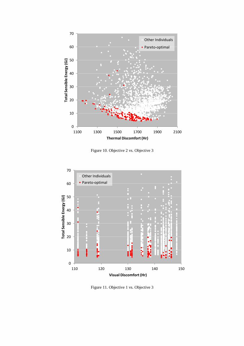
Figure 10. Objective 2 vs. Objective 3
Figure 11. Objective 1 vs. Objective 3
0
10
20
30
40
50
60
70
1100 1300 1500 1700 1900 2100
Tota
l Se
nsi
ble
En
erg
y (G
J)
Thermal Discomfort (Hr)
Other Individuals
Pareto-optimal
0
10
20
30
40
50
60
70
110 120 130 140 150
Tota
l Se
nsi
ble
En
ergy
(G
J)
Visual Discomfort (Hr)
Other Individuals
Pareto-optimal
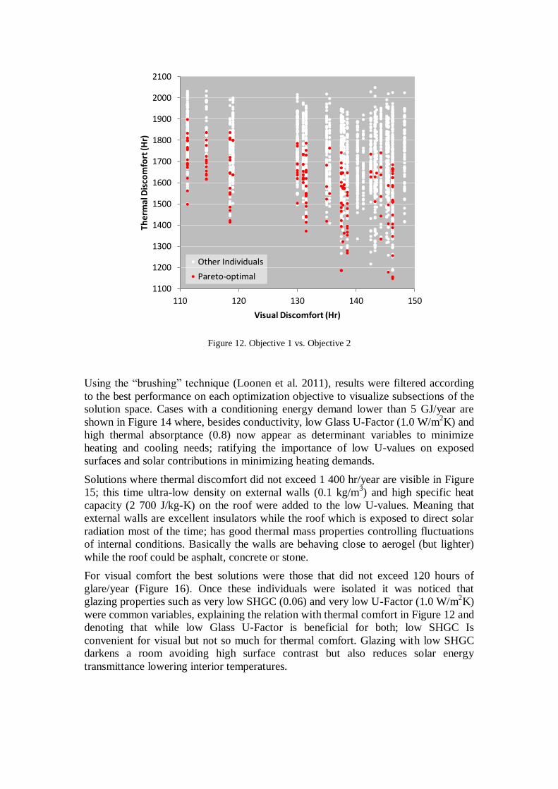
Figure 12. Objective 1 vs. Objective 2
Using the “brushing” technique (Loonen et al. 2011), results were filtered according
to the best performance on each optimization objective to visualize subsections of the
solution space. Cases with a conditioning energy demand lower than 5 GJ/year are
shown in Figure 14 where, besides conductivity, low Glass U-Factor (1.0 W/m2K) and
high thermal absorptance (0.8) now appear as determinant variables to minimize
heating and cooling needs; ratifying the importance of low U-values on exposed
surfaces and solar contributions in minimizing heating demands.
Solutions where thermal discomfort did not exceed 1 400 hr/year are visible in Figure
15; this time ultra-low density on external walls (0.1 kg/m3) and high specific heat
capacity (2 700 J/kg-K) on the roof were added to the low U-values. Meaning that
external walls are excellent insulators while the roof which is exposed to direct solar
radiation most of the time; has good thermal mass properties controlling fluctuations
of internal conditions. Basically the walls are behaving close to aerogel (but lighter)
while the roof could be asphalt, concrete or stone.
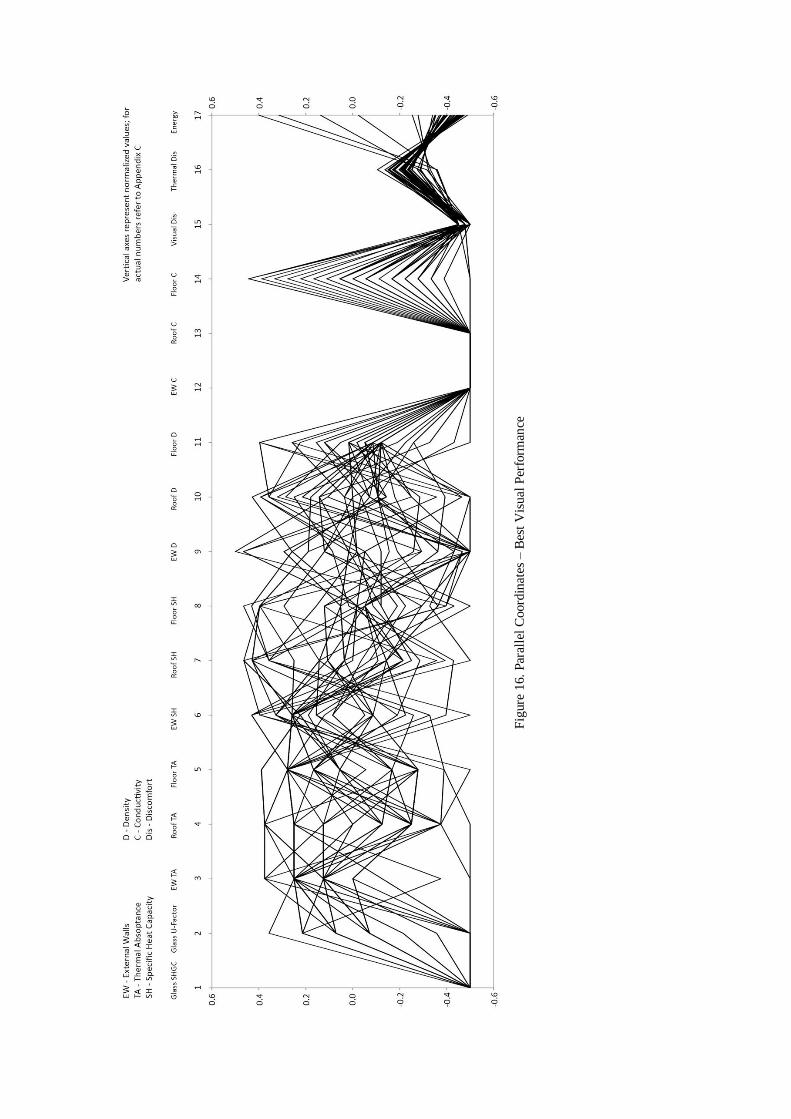
For visual comfort the best solutions were those that did not exceed 120 hours of
glare/year (Figure 16). Once these individuals were isolated it was noticed that
glazing properties such as very low SHGC (0.06) and very low U-Factor (1.0 W/m2K)
were common variables, explaining the relation with thermal comfort in Figure 12 and
denoting that while low Glass U-Factor is beneficial for both; low SHGC Is
convenient for visual but not so much for thermal comfort. Glazing with low SHGC
darkens a room avoiding high surface contrast but also reduces solar energy
transmittance lowering interior temperatures.
1100
1200
1300
1400
1500
1600
1700
1800
1900
2000
2100
110 120 130 140 150
The
rmal
Dis
com
fort
(Hr)
Visual Discomfort (Hr)
Other Individuals
Pareto-optimal

Fig
ure
13.
Par
alle
l C
oord
inat
es –
Par
eto O
pti
mal

Fig
ure
14.
Par
alle
l C
oord
inat
es –
Bes
t E
ner
gy
Per
form
ance

Fig
ure
15.
Par
alle
l C
oord
inat
es –
Bes
t T
her
mal
Per
form
ance
Fig
ure
16.
Par
alle
l C
oord
inat
es –
Bes
t V
isu
al P
erfo
rman
ce

To properly visualize results; the solution space was plotted in a tridimensional chart
picturing the three optimization objectives simultaneously. Dimension Z represents
energy, X visual comfort and Y thermal comfort while the gradient scheme indicates
where each solution stands in respect to Z with the green colour highlighting Pareto
individuals. It is noted that solutions displace parallel to the Y axis in a series of
curved rows that reduce as Y values get lower and where optimal solutions lie at the
bottom of each row ranging from high to low energy consumption due to the trade-off
dilemma previously described.
Figure 17. Tridimensional Solution Space

5. Ideal Dynamic Behaviour
In the first step using multi-objective optimization, those fabric properties offering the
best performance were revealed along with the trade-off dilemma that exemplifies the
inability to meet the objectives simultaneously. Results showed a set of solutions with
remarkable performance representing the best that a static building could accomplish.
Whereas static buildings can only offer optimal conditions for a limited amount of
time; the Ideal dynamic building should be able to have the best fabric properties
under any given condition thanks to its mutating ability. The objective of this second
step is therefore to find the dynamic behaviour that a building with the conditions
described in section 3.2 should have to improve its performance beyond the set of
Pareto solutions.
5.1. Building the Fabric
Weather and internal gain inputs at a given timestep possess individual characteristics
that would require different material parameters to obtain zero discomfort and energy
consumption all the time; basically each timestep needs to be optimized. This could
have been done using MOO but running the design space for a period of one hour
instead of a year, although it would have signified running 8 760 optimization jobs
each one containing 2 500 runs, resulting in 2.19x10⁷ simulations and requiring a total
20 411 hours. With this limitation a simplified approach was used where timesteps of
the best static buildings were combined to create a dynamic fabric capable to offer
optimal performance at each hour of the year. The difficulty relied on how to choose
which jobs were the best among the Pareto front as they are all best solutions and no
one is better than the other.
Three ranking methods were analysed; the first weighted solutions according to a
personal preference where energy consumption was considered the first priority
followed by thermal comfort with visual comfort being least important as it would be
manageable through blinds or louvers. Jobs where the three objectives had values
below the average were filtered obtaining a new list of 17 solutions. A tabular view of
the minimum, maximum and average values possible to obtain with this ranking
demonstrated that the best possible value for each objective would not be achieved if
these jobs were picked as parent ones and the dynamic building would not be the best
it could be (See Table 4). A second option used the logic behind the performance
indicators set-up, where the objective function was minimized for all three targets
meaning that the closer results were to zero, the better the performance would be.
Results were added and sorted in ascending order choosing the first five to represent
the best solutions. A tabular evaluation showed that with this approach the minimum
possible value for visual comfort and energy consumption would not be possible.
Other method used the ranking order proposed by the evolutionary algorithm taking
the first five as the best solutions for; as it was mentioned in section 4, the ranking
method for most MOO software encapsulates the tricks. The tabular evaluation
showed that the maximum and minimum values were included in this sample and that
their average was very similar to that of the whole Pareto set. This demonstrated that
the combination of these five jobs would generate the best dynamic building
behaviour.

Table 4. Ranking Tabular View
Visual (Hr) Thermal (Hr) Energy (GJ) Jobs
Max 146.25 1897.75 42.14
Min 111.25 1147.25 4.23
Average 131.39 1584.43 9.13
Max 138.50 1584.25 9.04
Min 131.50 1478.00 6.20
Average 136.53 1549.87 7.78
Max 146.25 1187.50 19.62
Min 137.50 1147.25 17.37
Average 144.35 1164.10 19.06
Max 146.25 1897.75 42.14
Min 111.25 1147.25 4.23
Average 131.85 1558.50 15.67
EAs Ranking
168
17
5
Ranking Method
Close to Zero 5
Pareto set
Above Average
These five jobs were simulated now in timesteps of one hour, to select which
properties to use for the ideal fabric behaviour the “close to zero” method was used. If
the sum of the objectives equal zero then that timestep could be considered ideal, in
the case more than one job presented the same ideal timestep then the priority would
be according to the EAs ranking while if the sum was different than zero then the
timestep with the lowest value would be chosen.
5.2. Dynamic Building Results
The percentage of the year parent jobs achieved ideal conditions ranged from 61% to
69%; by having the capacity to adapt its fabric properties the new building exhibited
ideal conditions along 75% of the year (See Table 5). When comparing annual energy
consumption and comfort performance (See Figure 18), the difficulty to balance
conflictive criteria with a static design is noticeable; case 4 exhibits the most balanced
performance but whereas thermal discomfort is the best possible value; visual
discomfort is the worst case condition. With the dynamic fabric the resulting heating
demand was 21.01 GJ/yr while cooling was completely eliminated for a total energy
consumption of 437.81 MJ/m2. Thermal discomfort was reduced to 880.75 hr/yr and
visual discomfort to 111.75 hr/yr. Even thou this solution do not have the lowest
energy consumption; it surely represents the best trade-off harmony and percentage of
ideal conditions along the year. The Pareto front is a better way to visualize the
dynamic building against the best static designs (See Figure 19), its location definitely
denotes improved behaviour although it seems that reaching the utopia point
described in (Boer et al. 2011) in which optimal comfort is achievable without
conflicting with energy consumption remains Zeno’s dichotomy paradox.
Table 5. Static Parents vs. Dynamic Fabric
0 1 2 3 4
Ideal Timesteps % 61% 71% 69% 71% 68% 75%
Visual Dis (Hr) 111.25 146.25 111.25 144.25 146.25 111.75
Thermal Dis (Hr) 1498 1508.5 1897.75 1741 1147.25 880.75
Heating GJ/yr 38.78 6.81 5.66 4.23 19.21 21.01
Cooling GJ/yr 3.37 0.00 0.02 0.00 0.28 0.00
Dynamic
Fabric
EAs RankObjective
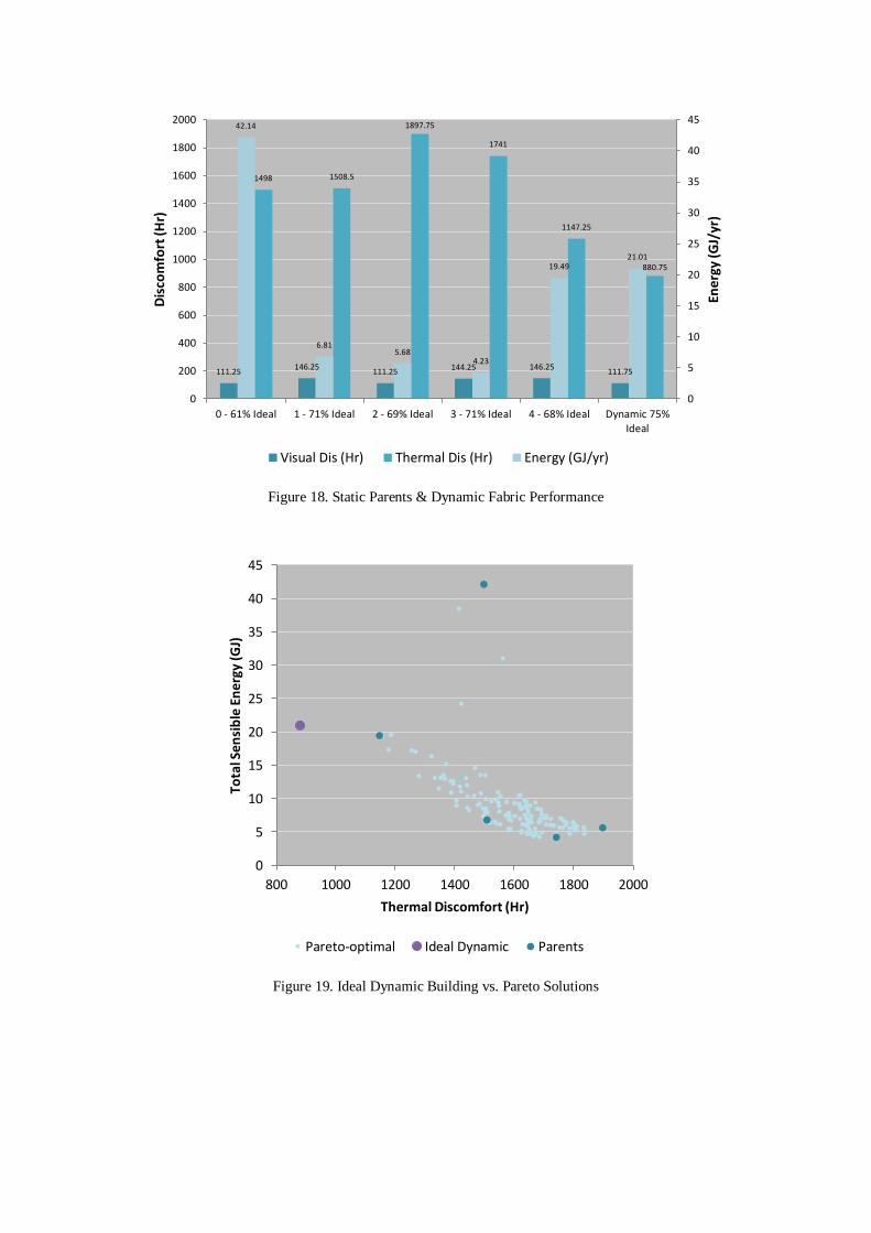
Figure 18. Static Parents & Dynamic Fabric Performance
Figure 19. Ideal Dynamic Building vs. Pareto Solutions
111.25 146.25
111.25 144.25 146.25
111.75
1498 1508.5
1897.75
1741
1147.25
880.75
42.14
6.81 5.68
4.23
19.49 21.01
0
5
10
15
20
25
30
35
40
45
0
200
400
600
800
1000
1200
1400
1600
1800
2000
0 - 61% Ideal 1 - 71% Ideal 2 - 69% Ideal 3 - 71% Ideal 4 - 68% Ideal Dynamic 75%Ideal
Ene
rgy
(GJ/
yr)
Dis
com
fort
(Hr)
Visual Dis (Hr) Thermal Dis (Hr) Energy (GJ/yr)
0
5
10
15
20
25
30
35
40
45
800 1000 1200 1400 1600 1800 2000
Tota
l Se
nsi
ble
En
ergy
(G
J)
Thermal Discomfort (Hr)
Pareto-optimal Ideal Dynamic Parents

6. Conclusions
Pursuing a sustainable built environment requires designers to be able to find an
optimal design efficiently. Evolutionary optimization allows Pareto solutions to be
identified in a single run whereas conventional trial-and-error methods can hardly
come up with the best possible solution. Despite its potential, MOO is not being
widely used from the conceptual design phase due to the lack of Architect-friendly
tools. Moreover building adaptation is a field in which the boundary between
professions gets blurry requiring knowledge beyond what Architecture and
Engineering commonly offer with close collaboration from disciplines like Chemistry,
Programming and Cybernetics amongst others.
Building performance simulation stands as an indispensable tool to evaluate adaptive
behaviours but current software specialize in the analysis of a certain physical domain
(Thermal, Visual, Moisture, Acoustic or Indoor Air Quality) with very few exceptions
covering a wider range and usually not strong in all. The domain interaction of
adaptive buildings inevitably demands performance analysis using different tools
presenting simulation coupling as an inevitable step.
Whereas most tools today include dynamic controls for shading and glazing; thermal
mass variability still represents the biggest challenge to simulate dynamic conditions
requiring advance simulation knowledge and creativity from the person that uses it
(Loonen 2010). Fortunately research in this field is starting to reflect; EnergyPlus for
example now allows total custom control of the envelope through the Energy
Management System (EMS) feature, representing a significant improvement though
there is still work needed to overcome the limitations of what software accept as
realistic.
The results presented indicate that adaptive behaviour in buildings stand as a
promising way to harmonize energy consumption and discomfort levels conflictive
nature. Further work would need to evaluate visual discomfort according to
illuminance levels instead of the glare index and include electric lighting control into
the simulation settings, dimming lights according to daylight contributions and
include their electricity use into the energy objective. This way energy consumption
would be affected by both comfort indicators closing the relationship between the
three variables. An additional step is to translate the analysis into a design proposal
and employ a dynamic simulation to compare how close it gets to the ideal behaviour
and validate the black box method as an architectural design principle.
References
Addington, M. & Schodek, D., 2005. Smart Materials and New Technologies: For
Architecture and Design Professions, Amsterdam: Elsevier.
An, L. et al., 2012. Estimation of Thermal Parameters of Buildings Through Inverse
Modeling and Clustering for a Portfolio of Buildings. In 5th National Conference
of IBPSA-USA. Madison, Wisconsin, pp. 295–305.
Aschehoug, Ø. & Perino, M., 2009. Expert Guide Part 2 Responsive Building
Elements, Norway, Italy.
Bakker, L. et al., 2009. Climate Adaptive Building Shells. TVVL Magazine, (3), pp.6
– 11.
Boer, B. De et al., 2011. Climate Adaptive Building Shells for the future –
Optimization with an Inverse Modelling Approach. In European Council for an
Energy Efficient Economy Summer Study. Presqu’île de Giens, France, pp. 1413–
1422.
De Boer, B., FACET: Facade as Adaptive Comfort-enhancing and Energy-saving
Future concept. Available at: http://www.eosfacet.nl/en/ [Accessed June 27,
2013].
Boer, B. De et al., 2012. Future Climate Adaptive Building Shells: Optimizing Energy
and Comfort by Inverse Modelling. In 8th Energy Forum on Solar Building
Skins. Bressanone, Italy, pp. 15–19.
Bunge, M., 1963. A General Black Box Theory. Philisophy of Science, 30(4), pp.346–
358.
Crespo, A. de A., 2007. Conceptual Design of a Building with Movable Parts.
Massachusetts Institute of Technology.
Drake, S., 2007. The third skin: architecture, technology & Enviroment, Sydney,
Australia: UNSW Press.
EnergyPlus, 2013a. EnergyPlus Engineering Reference: The Reference to EnergyPlus
Calculations. , pp.i – 1348.
EnergyPlus, 2013b. Input Output Reference The Encyclopedic Reference to
EnergyPlus Input and Output. , pp.i–1968.
Foerster, H. Von, 2003. Understanding Understanding: Essays On Cybernetics and
Cognition, Springer.
Glynn, R., 2008. The Wonder of Trivial Machines. Protoarchitecture: Analogue and
Digital Hybrids, 78(4), pp.13–21.
Heiselberg, P., 2012. ECBCS Annex 44 Integrating Environmentally Responsive
Elements in Buildings Project Summary Report, Denmark.
Heiselberg, P., 2009. Expert Guide Part 1 Responsive Building Concepts, Denmark.
Available at: www.civil.aau.dk/Annex44.
Johnson, E.A. & Kulesza, J.D., 2007. System for Allergen Reduction Through Indoor
Humidity Control. , 1(12), pp.1–12.
Judkoff, R. & Neymark, J., 1995. International Energy Agency Building Energy
Simulation Test (BESTEST) and Diagnostic Method.
Lartigue, B., Lasternas, B. & Loftness, V., 2013. Multi-objective Optimization of
Building Envelope for Energy Consumption and Daylight. Indoor and Built
Environment. Available at:

http://ibe.sagepub.com/cgi/doi/10.1177/1420326X13480224 [Accessed August
21, 2013].
Loonen, R., Climate Adaptive Building Shells. Available at:
http://pinterest.com/CABSoverview/ [Accessed June 26, 2013].
Loonen, R. et al., 2013. Climate adaptive building shells : State-of-the-art and future
challenges. , 25, pp.483–493.
Loonen, R., 2010. Climate Adaptive Building Shells, What can we simulate?
Technische Universiteit Eindhoven.
Loonen, R., Trcka, M. & Hensen, J.L.., 2011. Exploring the Potential of Climate
Adaptive Building Shells. In 12th IBPSA Conference. Sydney, Australia, pp.
2148–2155.
Moloney, 2007. A Framework for the Design of Kinetic Facades. In A. Dong, A.
Vande, & J. S, eds. Computed-Aided Architectural Design Futures Conference.
Sydney, Australia: Springer.
Naboni, E. et al., 2013. Comparison of Conventional, Parametric and Evolutionary
Optimization Approaches for the Architectural Design of Nearly Zero Energy
Buildings. In 13th Int. IBPSA Conference. Chambery, France.
Reddy, T.A., 1989. Application of Dynamic Building Inverse Models to Three
Occupied Residences Monitored Non-Intrusively. In Thermal Performance of
Exterior Envelopes of Buildings IV. Orlando, Florida, pp. 654–669.
Schnadelback, H., 2010. Adaptive Architecture: A Conceptual Framework. In
MediaCityMediaCity. Weimar, Germany.
Sharma, S., Rangaiah, G.P. & Cheah, K.S., 2012. Multi-objective Optimization Using
MS Excel with an Application to Design of a Falling-film Evaporator System.
Food and Bioproducts Processing, 90(2), pp.123–134. Available at:
http://linkinghub.elsevier.com/retrieve/pii/S0960308511000125 [Accessed
August 22, 2013].
Simonson, C.J. et al., 2004. Potential for Hygroscopic Building Materials to Improve
Indoor Comfort and Air Quality in the Canadian Climate. In Buildings IX.
Clearwater Beach, Florida, pp. 1–15.
Vassela, A., 1983. Third Skin: Building Biology. International Permaculture Journal,
(14).
Velikov, K. & Thün, G., 2013. Responsive Building Envelopes: Characteristics and
Evolving Paradigms. In Design and construction of high-performance homes:
building envelopes, renewable energies and integrated practice. Routledge.

Wang, W., Zmeureanu, R. & Rivard, H., 2005. Applying Multi-Objective Genetic
Algorithms in Green Building Design Optimization. Building and Environment,
40(11), pp.1512–1525. Available at:
http://linkinghub.elsevier.com/retrieve/pii/S0360132304003439 [Accessed
August 7, 2013].
Wigginton, M. & Harris, J., 2002. Intelligent Skins, Elsevier Architectural Press.
Yazdani, M., Krymsky, Y. & Aweida, C., 2011. Responsive Skins. Available at:
http://yazdanistudioresearch.wordpress.com/ [Accessed August 8, 2013].
Zhang, Y., 2012. Use jEPlus as an Efficient Building Design Optimisation Tool. In
CIBSE ASHRAE Technical Symposium. London, UK, pp. 1–12.
Zhang, Y., Korolija, I. & Stuart, G., 2011. jEPlus. Available at:
http://www.iesd.dmu.ac.uk/~jeplus/wiki/doku.php?id=download:start.
Recommended