Small-angle X-ray scattering – a (mostly)theoretical introduction to the basics
András Wacha
Research Centre for Natural Sciences, Hungarian Academy of Sciences

Contents
IntroductionA bit of historyThe principle of scatteringSmall- and wide-angle scattering
BasicsScattering pattern and scattering curveScattering cross-sectionScattering variableScattering contrast
Basic relations of scatteringConnection between structure and scatteringPhase problemSpherically symmetric systemsThe Guinier ApproximationMulti-particle systems, size distributionPower-law scattering: the Porod regionThe pair density distribution function
Summary

History of (small-angle) scattering
“Even the ancient greeks. . . ”
Scattering: XVII-XIX. century (Huygens, Newton, Young,Fresnel. . . )
X-rays: 1895 (Wilhelm Konrad Röntgen)
X-ray diffraction on crystals: W.H. és W.L. Bragg (1912), M. vonLaue, P. Debye, P. Scherrer. . . (-1930)
First observation of small-angle scattering: P. Krishnamurti, B.E.Warren (kb. 1930)
Mathematical formalism and theory of small-angle scattering: AndréGuinier, Peter Debye, Otto Kratky, Günther Porod, Rolf Hosemann,Vittorio Luzzati (1940-1960)

The principle of scattering
Primary beam
Sample
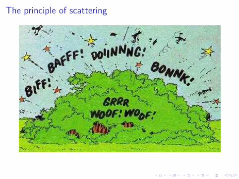
The principle of scattering
The principle of scattering

SAXS vs. WAXS
Principle of scattering: probe particles → interaction with thestructure → deflection → detection → structure determination
SampleX-ray Small-angle scattering
Wide-angle scattering (diffraction)
Measurement: the “intensity” of radiation deflected in differentdirections
Strong forward scattering (logarithmic scale!)
Wide-angle scattering: Bragg equation (cf. previous lecture)
Small-angle scattering: . . .

Small- and wide-angle X-ray scattering
Scattering of a spherical nanocrystallite (simple cubic lattice)
Wide-angle scattering: crystal structure
Small-angle scattering: the overall size of the crystallite Small-angle scattering is blind on the atomic level: equivalence of
homogeneous and discrete atomic structures
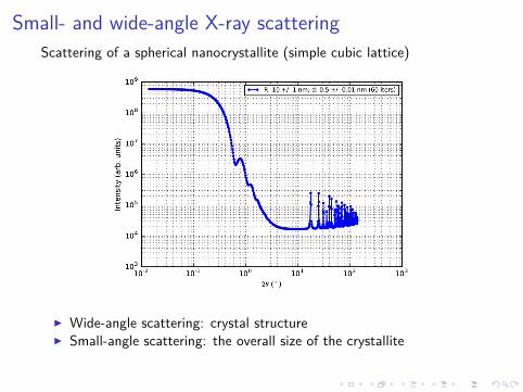
Small- and wide-angle X-ray scattering
Scattering of a spherical nanocrystallite (simple cubic lattice)
Wide-angle scattering: crystal structure Small-angle scattering: the overall size of the crystallite
Small-angle scattering is blind on the atomic level: equivalence ofhomogeneous and discrete atomic structures

Small- and wide-angle X-ray scattering
Scattering of a spherical nanocrystallite (simple cubic lattice)
Wide-angle scattering: crystal structure Small-angle scattering: the overall size of the crystallite Small-angle scattering is blind on the atomic level: equivalence of
homogeneous and discrete atomic structures

Small-angle scattering
Small-Angle X-ray Scattering – SAXS Elastic scattering of X-rays on electrons Measurement: “intensity” versus the scattering angle Results: electron-density inhomogeneities on the 1-100 length scale But: indirect results, difficult to interpret (/) Typical experimental conditions:
Transmission geometry High intensity, nearly point-collimated beam Two-dimensional position sensitive detector
Incident rays
Scattered rays Scattering pattern Scattering curve
Azimuthal
averaging
Beam stop
Unscattered + forward scattered
radiation
Scatterer
("sample")
0.1 1
0.001
0.01
0.1
1
10
100
q (1/nm)In
tensit
y (1
/cm
× 1
/sr)

Contents
IntroductionA bit of historyThe principle of scatteringSmall- and wide-angle scattering
BasicsScattering pattern and scattering curveScattering cross-sectionScattering variableScattering contrast
Basic relations of scatteringConnection between structure and scatteringPhase problemSpherically symmetric systemsThe Guinier ApproximationMulti-particle systems, size distributionPower-law scattering: the Porod regionThe pair density distribution function
Summary
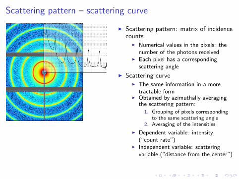
Scattering pattern – scattering curve
Scattering pattern: matrix of incidencecounts
Numerical values in the pixels: thenumber of the photons received
Each pixel has a correspondingscattering angle
Scattering curve The same information in a more
tractable form Obtained by azimuthally averaging
the scattering pattern:
1. Grouping of pixels correspondingto the same scattering angle
2. Averaging of the intensities
Dependent variable: intensity(“count rate”)
Independent variable: scatteringvariable (“distance from the center”)

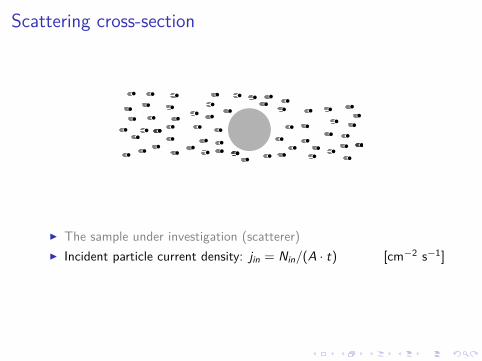
Scattering cross-section
The sample under investigation (scatterer)
Incident particle current density: jin = Nin (A · t) [cm−2 s−1]
Total scattered particle current: Iout = Nout t [s−1]
Scattering cross-section: Σ ≡ Iout jin = A · Nout Nin [cm2]
differential scattering cross-section: dΣ dΩ [cm2 sr−1]
Normalized to unit sample volume: ddΩ ≡ 1
VdΣdΩ [cm−1 sr−1]
Scattering cross-section
The sample under investigation (scatterer)
Incident particle current density: jin = Nin/(A · t) [cm−2 s−1]
Total scattered particle current: Iout = Nout t [s−1]
Scattering cross-section: Σ ≡ Iout jin = A · Nout Nin [cm2]
differential scattering cross-section: dΣ dΩ [cm2 sr−1]
Normalized to unit sample volume: ddΩ ≡ 1
VdΣdΩ [cm−1 sr−1]

Scattering cross-section
The sample under investigation (scatterer)
Incident particle current density: jin = Nin/(A · t) [cm−2 s−1]
Total scattered particle current: Iout = Nout/t [s−1]
Scattering cross-section: Σ ≡ Iout/jin = A · Nout/Nin [cm2]
differential scattering cross-section: dΣ/dΩ [cm2 sr−1]
Normalized to unit sample volume: dσdΩ ≡ 1
VdΣdΩ [cm−1 sr−1]

The scattering variable
The natural variable of the intensity is the scattering vector:
~q ≡ ~k2θ − ~k0
[
~s ≡ ~S2θ − ~S0 = ~q/(2π)]
i.e. the vectorial difference of the wave vectors of the scattered andthe incident radiation
[Wave vector: points in the direction of wave propagation,magnitude is 2π/λ]
Physical meaning: the momentum acquired by the photon uponscattering (→ “momentum transfer”)
|k0|=2π/λ
|k2θ|=
2π/λ
|q|=
4π sinθ
/ λ
|k0|=2π/λ2θ
Sample
Incident beam Forward scattering
Radiation sc
attere
d
under 2θ
Magnitude: q = |~q| = 4π sin θλ
≈small angles
4πθ/λ [s = 2 sin θ/λ])
Bragg-equation: q = 2πn/d n ∈ Z [s = n/d ]

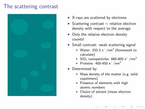
The scattering contrast
X-rays are scattered by electrons
Scattering contrast = relative electrondensity with respect to the average
Only the relative electron densitycounts!
Small contrast: weak scattering signal Water: 333.3 e−/nm3 (homework to
calculate) SiO2 nanoparticles: 660-800 e−/nm3
Proteins: 400-450 e−/nm3
Determined by: Mass density of the matter (e.g. solid
copolimers) Presence of elements with high
atomic numbers Choice of solvent (mean electron
density)

Recapitulation of the basic quantities
Intensity: or differential scattering cross-section
the proportion of the particles. . . . . . incoming in a unit cross section. . . . . . over unit time. . . . . . onto a sample of unit volume. . . . . . which is scattered in a given direction. . . . . . under unit solid angle.
Scattering variable (q): or momentum transfer: characterizing the angledependence.
Magnitude ∝ sin θ ≈ θ ~~q: the momentum acquired by the photon due to
the interaction with the sample
Scattering contrast: scattering potential of given part of the sample incomparison with its environment
This is the relative electron density in case of X-rayscattering

Contents
IntroductionA bit of historyThe principle of scatteringSmall- and wide-angle scattering
BasicsScattering pattern and scattering curveScattering cross-sectionScattering variableScattering contrast
Basic relations of scatteringConnection between structure and scatteringPhase problemSpherically symmetric systemsThe Guinier ApproximationMulti-particle systems, size distributionPower-law scattering: the Porod regionThe pair density distribution function
Summary

Connection between structure and scattering
Scattering on the inhomogeneities of the electron density ⇒characterization of the structure with the relative electron densityfunction:
∆ρ(~r) = ρ(~r) − ρ
(in the following we omit ∆!)
The amplitude of the scattered radiation:
A(~q) =y
V
ρ(~r)e−i~q~rd
3~r
which is formally the Fourier transform of the electron density.
Only the intensity can be measured: I = |A|2

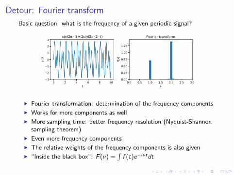
Detour: Fourier transform
Basic question: what is the frequency of a given periodic signal?
0 2 4 6 8 10t
1.0
0.5
0.0
0.5
1.0y(
t)sin(2 t)
0.0 0.5 1.0 1.5 2.00.0
0.2
0.4
0.6
[y]
Fourier transform
Fourier transformation: determination of the frequency components
W rks for more components as well
re sampling time: better frequency resolution (Nyquist-Shannonsampling theorem)
Even more frequency components
The relative weights of the frequency components is also given
“Inside the black b x”: F (ν) =∫
f (t)e−iνtdt
Can be inverted (although. . . ): f (t) = 12π
∫F (ν)e itνdν

Detour: Fourier transform
Basic question: what is the frequency of a given periodic signal?
0 2 4 6 8 10t
2
1
0
1
2y(
t)sin(2 t) + sin(2 1.1 t)
0.0 0.5 1.0 1.5 2.00.0
0.2
0.4
0.6
[y]
Fourier transform
Fourier transformation: determination of the frequency components
Works for more components as well
re sampling time: better frequency resolution (Nyquist-Shannonsampling theorem)
Even more frequency components
The relative weights of the frequency components is also given
“Inside the black b x”: F (ν) =∫
f (t)e−iνtdt
Can be inverted (although. . . ): f (t) = 12π
∫F (ν)e itνdν

Detour: Fourier transform
Basic question: what is the frequency of a given periodic signal?
0 10 20 30 40 50t
2
1
0
1
2y(
t)sin(2 t) + sin(2 1.1 t)
0.0 0.5 1.0 1.5 2.00.0
0.2
0.4
0.6
[y]
Fourier transform
Fourier transformation: determination of the frequency components
Works for more components as well
More sampling time: better frequency resolution (Nyquist-Shannonsampling theorem)
Even more frequency components
The relative weights of the frequency components is also given
“Inside the black b x”: F (ν) =∫
f (t)e−iνtdt
Can be inverted (although. . . ): f (t) = 12π
∫F (ν)e itνdν

Detour: Fourier transform
Basic question: what is the frequency of a given periodic signal?
0 10 20 30 40 50t
3
2
1
0
1
2
3y(
t)sin(2 0.9 t) + sin(2 t) + sin(2 1.1 t)
0.0 0.5 1.0 1.5 2.00.0
0.2
0.4
0.6
[y]
Fourier transform
Fourier transformation: determination of the frequency components
Works for more components as well
More sampling time: better frequency resolution (Nyquist-Shannonsampling theorem)
Even more frequency components
The relative weights of the frequency components is also given
“Inside the black b x”: F (ν) =∫
f (t)e−iνtdt
Can be inverted (although. . . ): f (t) = 12π
∫F (ν)e itνdν

Detour: Fourier transform
Basic question: what is the frequency of a given periodic signal?
0 2 4 6 8 10t
3
2
1
0
1
2
3y(
t)sin(2 t) + 2sin(2 2 t)
0.0 0.5 1.0 1.5 2.0 2.5 3.00.00
0.25
0.50
0.75
1.00
1.25
[y]
Fourier transform
Fourier transformation: determination of the frequency components
Works for more components as well
More sampling time: better frequency resolution (Nyquist-Shannonsampling theorem)
Even more frequency components
The relative weights of the frequency components is also given
“Inside the black b x”: F (ν) =∫
f (t)e−iνtdt
Can be inverted (although. . . ): f (t) = 12π
∫F (ν)e itνdν
Detour: Fourier transform
Basic question: what is the frequency of a given periodic signal?
0 2 4 6 8 10t
3
2
1
0
1
2
3y(
t)sin(2 t) + 2sin(2 2 t)
0.0 0.5 1.0 1.5 2.0 2.5 3.00.00
0.25
0.50
0.75
1.00
1.25
[y]
Fourier transform
Fourier transformation: determination of the frequency components
Works for more components as well
More sampling time: better frequency resolution (Nyquist-Shannonsampling theorem)
Even more frequency components
The relative weights of the frequency components is also given
“Inside the black box”: F (ν) =∫
f (t)e−iνtdt
Can be inverted (although. . . ): f (t) = 12π
∫F (ν)e itνdν

The phase problem
The Fourier transform is invertible (?!): the amplitudeunambiguously describes the scattering structure
Complex quantities:z = a + bi = Ae iφ
Absolute square (this is how we get the intensity):
|z |2 = z · z∗ = Ae iφ · Ae−iφ = A2
Where did the φ phase go?!
Because the scattered amplitude cannot be measured, there is nochance to fully recover the structure just from scattering.
Another problem: the intensity can only be measured in a subspaceof the ~q space: only an incomplete inversion of the Fourier transformcan be done.

How big is this problem?
Idea from Saldin et. al. J. Phys.: Condens. Matter 13 (2001) 10689-10707
The phase carries most of the information! The operation of taking the square root is ambiguous over the
complex plane (there are complex numbers with |z | = 1)!

How big is this problem?
FT
FT
Idea from Saldin et. al. J. Phys.: Condens. Matter 13 (2001) 10689-10707
The phase carries most of the information! The operation of taking the square root is ambiguous over the
complex plane (there are complex numbers with |z | = 1)!

How big is this problem?
FT
FT
Amplitude
(Kratky)
Amplitude
(Porod)
Phase
(Kratky)
Phase
(Porod)
IFT
IFT
Idea from Saldin et. al. J. Phys.: Condens. Matter 13 (2001) 10689-10707
The phase carries most of the information!
The operation of taking the square root is ambiguous over thecomplex plane (there are complex numbers with |z | = 1)!

How big is this problem?
Re
Im
z |z|2=1
1
i
The phase carries most of the information!
The operation of taking the square root is ambiguous over thecomplex plane (there are ∞ complex numbers with |z | = 1)!

What can be done / Is this really a problem?
The scattering of vastly different structures can be undiscernible1. Solution: determination of “robust” parameters (see later)
Guinier radius Power-law exponent Porod-volume . . .
2. Solution: model fitting Choosing the specimen from a model-specimen described by given
parameters which best fits the scattering curve If the model ensemble is narrow enough, the ρ(~r) ↔ I(~q) mapping
can be unique A priori knowledge, results of other experiments are indispensable!
3. “Guessing” the phase (crystallography) or measuring it (holography)
Structures which
are compatible with
the measured data
Structures which
can be parametrized
by the model

Bragg’s law: a special case
The sample is periodic (drepeat distance)
θ: incidence and exit angle
Constructive interference in thedetector: the rays reflectedfrom neighbouring planes reachthe detector in phase
Path difference: ∆s = nλwhere n ∈ N
From simple geometry:∆s = 2d sin θ
2d sin θ = nλ
4πλ
sin θ = 2πd
n
q =2π
dn
θ
θθ
θ
Δsd
λ

Detour/recap: spherical coordinates
Descartes: x , y , z
Spherical: x = r sin θ cos ϕ, y = r sin θ sin ϕ, z = r cos θ
Infinitesimal volume:
dx dy dz = dV = r2 sin θ dr dθ dϕ
Integral:
∞∫
−∞
∞∫
−∞
∞∫
−∞
f (x , y , z)dx dy dz =
=
2π∫
0
π∫
0
∞∫
0
f (r , θ, ϕ)r2 sin θdr dθ dϕx
y
z
r
θ
φ
dr
dθ
dφ

Small-angle scattering of a sphere (I)
General formula of the scattered intensity:
I(~q) =∣∣∣
yρ (~r) e−i~q~r
d3~r
∣∣∣
2
Let us derive the (small-angle) scattering intensity of a sphere which hasa radius R and 0 homogeneous electron density inside!Electron-density function of an isotropic object: (r) = (|r |) = (r).The integral can be simpified in spherical co rdinates:
I(q) =
∣∣∣∣
∫ 2π
0
dφ
∫ ∞
0
dr r2 (r)
∫ π
0
sin θ dθ e−i|~q|·|~r | cos θ
∣∣∣∣
2
where z has been chosen to be parallel with q (can be done due to thespherical symmetry of (r))Substitution of u = cos θ:
I(q) =
∣∣∣∣∣∣∣∣
∫ 2π
0
dφ
2π
∫ ∞
0
r2 (r)dr
∫ 1
−1
du e−iqru
∣∣∣∣∣∣∣∣
2

Small-angle scattering of a sphere (I)
General formula of the scattered intensity:
I(~q) =∣∣∣
yρ (~r) e−i~q~r
d3~r
∣∣∣
2
Let us derive the (small-angle) scattering intensity of a sphere which hasa radius R and ρ0 homogeneous electron density inside!
Electron-density function of an isotropic object: (r) = (|r |) = (r).The integral can be simpified in spherical co rdinates:
I(q) =
∣∣∣∣
∫ 2π
0
dφ
∫ ∞
0
dr r2 (r)
∫ π
0
sin θ dθ e−i|~q|·|~r | cos θ
∣∣∣∣
2
where z has been chosen to be parallel with q (can be done due to thespherical symmetry of (r))Substitution of u = cos θ:
I(q) =
∣∣∣∣∣∣∣∣
∫ 2π
0
dφ
2π
∫ ∞
0
r2 (r)dr
∫ 1
−1
du e−iqru
∣∣∣∣∣∣∣∣
2

Small-angle scattering of a sphere (I)
General formula of the scattered intensity:
I(~q) =∣∣∣
yρ (~r) e−i~q~r
d3~r
∣∣∣
2
Let us derive the (small-angle) scattering intensity of a sphere which hasa radius R and ρ0 homogeneous electron density inside!Electron-density function of an isotropic object: ρ(~r) = ρ(|~r |) = ρ(r).The integral can be simpified in spherical coordinates:
I(~q) =
∣∣∣∣
∫ 2π
0
dφ
∫ ∞
0
dr r2ρ(r)
∫ π
0
sin θ dθ e−i|~q|·|~r | cos θ
∣∣∣∣
2
where z has been chosen to be parallel with ~q (can be done due to thespherical symmetry of ρ(~r))
Substitution of u = cos θ:
I(q) =
∣∣∣∣∣∣∣∣
∫ 2π
0
dφ
2π
∫ ∞
0
r2 (r)dr
∫ 1
−1
du e−iqru
∣∣∣∣∣∣∣∣
2

Small-angle scattering of a sphere (I)
General formula of the scattered intensity:
I(~q) =∣∣∣
yρ (~r) e−i~q~r
d3~r
∣∣∣
2
Let us derive the (small-angle) scattering intensity of a sphere which hasa radius R and ρ0 homogeneous electron density inside!Electron-density function of an isotropic object: ρ(~r) = ρ(|~r |) = ρ(r).The integral can be simpified in spherical coordinates:
I(~q) =
∣∣∣∣
∫ 2π
0
dφ
∫ ∞
0
dr r2ρ(r)
∫ π
0
sin θ dθ e−i|~q|·|~r | cos θ
∣∣∣∣
2
where z has been chosen to be parallel with ~q (can be done due to thespherical symmetry of ρ(~r))Substitution of u = cos θ:
I(~q) =
∣∣∣∣∣∣∣∣
∫ 2π
0
dφ
︸ ︷︷ ︸
2π
∫ ∞
0
r2ρ(r)dr
∫ 1
−1
du e−iqru
∣∣∣∣∣∣∣∣
2

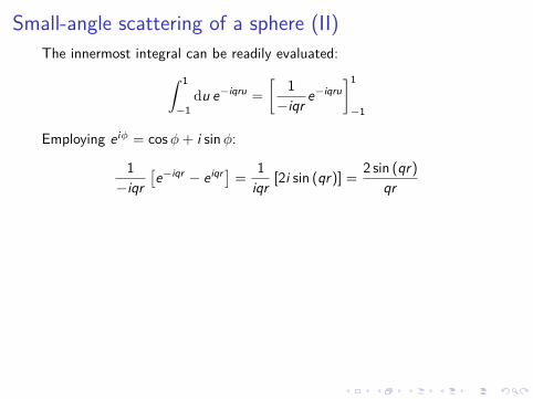
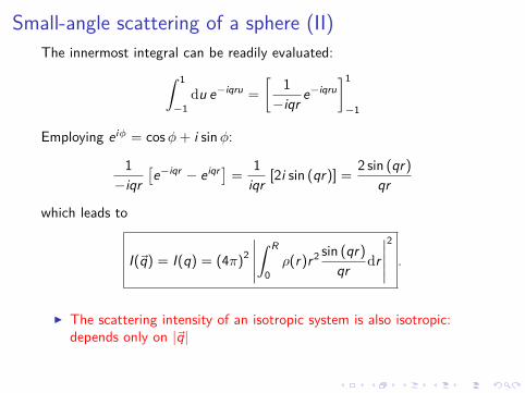
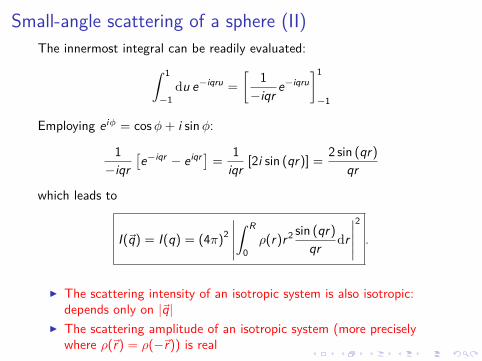
Small-angle scattering of a sphere (II)
The innermost integral can be readily evaluated:
∫ 1
−1
du e−iqru =
[1
−iqre−iqru
]1
−1
Employing e iφ = cos φ + i sin φ:
−iqr
[e−iqr − e iqr
]=
iqr[ i sin (qr)] =
sin (qr)
qr
which leads to
I(q) = I(q) = ( π)2
∣∣∣∣∣
∫
0
(r)r2 sin (qr)
qrdr
∣∣∣∣∣
2
.
The scattering intensity of an isotropic system is also isotropic:depends only on |q|
The scattering amplitude of an isotropic system (more preciselywhere (r) = (−r)) is real
Small-angle scattering of a sphere (II)
The innermost integral can be readily evaluated:
∫ 1
−1
du e−iqru =
[1
−iqre−iqru
]1
−1
Employing e iφ = cos φ + i sin φ:
1
−iqr
[e−iqr − e iqr
]=
1
iqr[2i sin (qr)] =
2 sin (qr)
qr
which leads to
I(q) = I(q) = ( π)2
∣∣∣∣∣
∫
0
(r)r2 sin (qr)
qrdr
∣∣∣∣∣
2
.
The scattering intensity of an isotropic system is also isotropic:depends only on |q|
The scattering amplitude of an isotropic system (more preciselywhere (r) = (−r)) is real

Small-angle scattering of a sphere (II)
The innermost integral can be readily evaluated:
∫ 1
−1
du e−iqru =
[1
−iqre−iqru
]1
−1
Employing e iφ = cos φ + i sin φ:
1
−iqr
[e−iqr − e iqr
]=
1
iqr[2i sin (qr)] =
2 sin (qr)
qr
which leads to
I(~q) = I(q) = (4π)2
∣∣∣∣∣
∫ R
0
ρ(r)r2 sin (qr)
qrdr
∣∣∣∣∣
2
.
The scattering intensity of an isotropic system is also isotropic:depends only on |q|
The scattering amplitude of an isotropic system (more preciselywhere (r) = (−r)) is real
Small-angle scattering of a sphere (II)
The innermost integral can be readily evaluated:
∫ 1
−1
du e−iqru =
[1
−iqre−iqru
]1
−1
Employing e iφ = cos φ + i sin φ:
1
−iqr
[e−iqr − e iqr
]=
1
iqr[2i sin (qr)] =
2 sin (qr)
qr
which leads to
I(~q) = I(q) = (4π)2
∣∣∣∣∣
∫ R
0
ρ(r)r2 sin (qr)
qrdr
∣∣∣∣∣
2
.
The scattering intensity of an isotropic system is also isotropic:depends only on |~q|
The scattering amplitude of an isotropic system (more preciselywhere ρ(~r) = ρ(−~r)) is real

Small-angle scattering of a sphere (III)
The electron-density function of a homogeneous sphere is:
ρ(~r) =
ρ0 if |~r | ≤ R
0 otherwise.
Evaluating the previous integral:
Ig(q) =
(4πρ0
q3(sin(qR) − qR cos(qR))
)2
= ρ20
4πR3
3︸ ︷︷ ︸
V
3
q3R3(sin(qR) − qR cos(qR))
︸ ︷︷ ︸
Pg (qR)
2
The scattered intensity scales with the 6th power of the linear size(I ∝ V 2 ∝ R6)
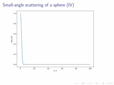
Small-angle scattering of a sphere (IV)
0 20 40 60 80 100q R
0.0
0.2
0.4
0.6
0.8
1.0|P(q
R)|2
Log-log plotting is d , qR < approximation: I ≈ e− q2 2
5 (Guinier)

Small-angle scattering of a sphere (IV)
10 1 100 101 102
q R
10 11
10 9
10 7
10 5
10 3
10 1
|P(q
R)|2
Log-log plotting is good ,
qR < approximation: I ≈ e− q2 2
5 (Guinier)
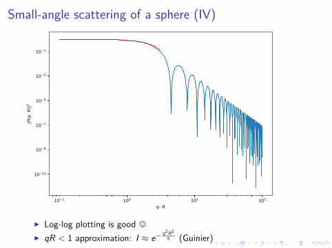
Small-angle scattering of a sphere (IV)
10 1 100 101 102
q R
10 11
10 9
10 7
10 5
10 3
10 1
|P(q
R)|2
Log-log plotting is good , qR < 1 approximation: I ≈ e− q2R2
5 (Guinier)

Small-angle scattering of a sphere (IV)
10 1 100
q R
10 1
100
|P(q
R)|2
Log-log plotting is good , qR < 1 approximation: I ≈ e− q2R2
5 (Guinier)

The Guinier approximation
André Guinier: the low-q scattering of dilute nanoparticlesuspensions follows a Gaussian curve
Generally:
I(q ≈ 0) = I0e−q2R2
g3
Radius of gyration (or Guinier radius): describes the linear size of ascattering object. By definition:
Rg ≡
√tV
r2ρ(~r)d3~rtV
ρ(~r)d3~r
Connection between the shape parameters and Rg :
sphere: Rg =√
3/5R spherical shell: Rg = R
cylinder:
√R2
2+ L2
12
linear polymer chain: Nb2/6 . . .

Guinier plot
10-1
q (nm−1)
105
106
107
108
109
Inte
nsit
y (
arb
. unit
s)
Simulated data
Rg=16.3 nm
I ≈ I0e−q2R2
g3
ln I ≈ ln I0 −2g
3 q2
ln I - q2: first rder polynomial
Visual check on the validity of the Guinier approximation

Guinier plot
10-1
q (nm−1)
105
106
107
108
109
Inte
nsit
y (
arb
. unit
s)
Simulated data
Rg=16.3 nm
I ≈ I0e−q2R2
g3
ln I ≈ ln I0 −R2
g
3 q2
ln I - q2: first rder polynomial
Visual check on the validity of the Guinier approximation

Guinier plot
0.05 0.10 0.15 0.20
q (nm−1)
107
108
109
Inte
nsit
y (
arb
. unit
s)
Simulated data
Rg=16.3 nm
I ≈ I0e−q2R2
g3
ln I ≈ ln I0 −R2
g
3 q2
ln I - q2: first order polynomial
Visual check on the validity of the Guinier approximation

The validity of the Guinier approximation
The Guinier approximationholds for nearly monodisperse
particulate systems too (seenext slides)
Nearly spherical particles:qRg / 3
Anisotropic particles:qRg / 0.7
Upturn at small q (“smilingGuinier”): attraction betweenthe particles (aggregation)
Downturn at small q (“frowningGuinier”): repulsive interactionbetween the particles
More details will be given forprotein scattering later. . .
André Guinier (1911 - 2000)

The effect of polydispersity
Multi-particle system:
ρ(~r) =∑
j
ρj(~r − ~Rj)
Scattering amplitude:
A(~q) =∑
j
Aj(~q)
=∑
j
Aj,0(~q)e−i~q~Rj
Intensity:
I(~q) = A(~q)A∗(~q)
=∑
j
∑
k
Aj(~q)A∗k(~q)e i~q(~Rk −~Rj )
Shifting of the electron densityfunction by ~R:
Ashifted(~q) = A0(~q)e−i~q~R
r r'R1
R2
R3Rj
RN

Multi-particle system
I(~q) =∑
j
∑
k
Aj(~q)A∗k(~q)e i~q(~Rk −~Rj ) =
∑
j
Ij(~q)
︸ ︷︷ ︸
incoherent
+∑
j
∑
k 6=j
Aj(~q)A∗k(~q)e i~q(~Rk −~Rj )
︸ ︷︷ ︸
interference term
Incoherent sum: the intensity of the distinct particles is summarized Cross-terms: interference from the correlated relative positions of
the particles Special case: identical, spherically symmetric particles
I(q) = ρ20V 2Pg (qR)2N
1 +
2
N
∑
j
∑
k>j
cos(
~q(~Rk − ~Rj))
︸ ︷︷ ︸
S(q)
Structure factor: depends only on the relative positions of thedistinct particles but not on their shape
Uncorrelated system: S(q) = 1. Otherwise the Guinier region isdistorted!

Size distribution
There’s no such thing as a fully monodisperse system.
10 1 100
q (nm 1)
104
105
106
107
108
109
1010
1011
Inte
nsity
(arb
. uni
ts)
R= 40 nmAverage

Size distribution
There’s no such thing as a fully monodisperse system.
10 1 100
q (nm 1)
104
105
106
107
108
109
1010
1011
Inte
nsity
(arb
. uni
ts)
R= 37 nmR= 43 nmAverage

Size distribution
There’s no such thing as a fully monodisperse system.
10 1 100
q (nm 1)
104
105
106
107
108
109
1010
1011
Inte
nsity
(arb
. uni
ts)
R= 37 nmR= 40 nmR= 43 nmAverage

Size distribution
There’s no such thing as a fully monodisperse system.
10 1 100
q (nm 1)
104
105
106
107
108
109
1010
1011
Inte
nsity
(arb
. uni
ts)
R= 36 nmR= 37 nmR= 38 nmR= 39 nmR= 40 nmR= 41 nmR= 42 nmR= 43 nmAverage

Scattering of a slightly polydisperse suspension ofnanoparticles
Scattering of a dilute nanoparticle suspension:
I(q) =
∫ ∞
0
P(R)
size distribution
· 20
contrast
· V
volume
2 ·
P2(qR)︸ ︷︷ ︸
form factor
dR
If the shape of the particles is known, the size distribution can bedetermined by fitting the scattering curve.
0.1 1
q (1/nm)
10-1
100
101
102
dΣ/dΩ
(cm
−1 s
r−1)
SiO2 ⊘ 34.6 nm
26 28 30 32 34 36 38 40 42
Diameter (nm)
Rela
tive f
requency
(arb
. unit
s) SAXS
TEM
Statistically significant (≈ 109 particles in 1 mm3) Accurate sizes with well-defined uncertainties (SI “traceability”)

Scattering of a slightly polydisperse suspension ofnanoparticles
Scattering of a dilute nanoparticle suspension:
I(q) =
∫ ∞
0
P(R)
size distribution
· 20
contrast
·
VR︸︷︷︸
volume
2 · P2(qR)︸ ︷︷ ︸
form factor
dR
If the shape of the particles is known, the size distribution can bedetermined by fitting the scattering curve.
0.1 1
q (1/nm)
10-1
100
101
102
dΣ/dΩ
(cm
−1 s
r−1)
SiO2 ⊘ 34.6 nm
26 28 30 32 34 36 38 40 42
Diameter (nm)
Rela
tive f
requency
(arb
. unit
s) SAXS
TEM
Statistically significant (≈ 109 particles in 1 mm3) Accurate sizes with well-defined uncertainties (SI “traceability”)

Scattering of a slightly polydisperse suspension ofnanoparticles
Scattering of a dilute nanoparticle suspension:
I(q) =
∫ ∞
0
P(R)
size distribution
·
ρ20
︸︷︷︸contrast
· VR︸︷︷︸
volume
2 · P2(qR)︸ ︷︷ ︸
form factor
dR
If the shape of the particles is known, the size distribution can bedetermined by fitting the scattering curve.
0.1 1
q (1/nm)
10-1
100
101
102
dΣ/dΩ
(cm
−1 s
r−1)
SiO2 ⊘ 34.6 nm
26 28 30 32 34 36 38 40 42
Diameter (nm)
Rela
tive f
requency
(arb
. unit
s) SAXS
TEM
Statistically significant (≈ 109 particles in 1 mm3) Accurate sizes with well-defined uncertainties (SI “traceability”)

Scattering of a slightly polydisperse suspension ofnanoparticles
Scattering of a dilute nanoparticle suspension:
I(q) =
∫ ∞
0
P(R)︸ ︷︷ ︸
size distribution
· ρ20
︸︷︷︸contrast
· VR︸︷︷︸
volume
2 · P2(qR)︸ ︷︷ ︸
form factor
dR
If the shape of the particles is known, the size distribution can bedetermined by fitting the scattering curve.
0.1 1
q (1/nm)
10-1
100
101
102
dΣ/dΩ
(cm
−1 s
r−1)
SiO2 ⊘ 34.6 nm
26 28 30 32 34 36 38 40 42
Diameter (nm)
Rela
tive f
requency
(arb
. unit
s) SAXS
TEM
Statistically significant (≈ 109 particles in 1 mm3) Accurate sizes with well-defined uncertainties (SI “traceability”)

Bimodal nanoparticle distribution

Model-independent approach
The P(R) size distribution function is obtained in a histogram form.
Large number of model parameters ⇒ danger of “overfitting”

Power-law behaviour
10 1 100
q (nm 1)
104
105
106
107
108
109
1010
1011
Inte
nsity
(arb
. uni
ts)
R= 36 nmR= 37 nmR= 38 nmR= 39 nmR= 40 nmR= 41 nmR= 42 nmR= 43 nmAverage
Power-law behaviour
10 1 100
q (nm 1)
104
105
106
107
108
109
1010
1011
Inte
nsity
(arb
. uni
ts)
R= 36 nmR= 37 nmR= 38 nmR= 39 nmR= 40 nmR= 41 nmR= 42 nmR= 43 nmAverageq 4
The Porod region
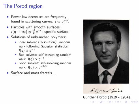
Power-law decreases are frequentlyfound in scattering curves: I ∝ q−α.
Particles with smooth surfaces:I(q → ∞) ∝ S
Vq−4: specific surface!
Solutions of unbranched polymers: Ideal solvent (Θ-solution): random
walk following Gaussian statistics:I(q) ∝ q−2
Bad solvent: self-attracting randomwalk: I(q) ∝ q−3
Good solvent: self-avoiding randomwalk: I(q) ∝ q−3/5
Surface and mass fractals. . .
Günther Porod (1919 - 1984)

Detour: fractals
Self-similar systems: showing the same shapes even in differentmagnifications
Nanosystems with fractal properties: Activated carbon Porous minerals Uneven surfaces
Characterization: Hausdorff-dimension (fractal dimension)

Fractal dimension
Measure the area of the Sierpińsky carpet with different unit lengths Connection between the unit length and the required unit areas to
cover the carpet:Length unit 1 1/3 1/9 . . . 3−n
Required unit areas 1 8 64 . . . 8n
A Hausdorff dimension: how the number of required unit areas (A)scales with the unit length (a)?
a = 1/3n → n = − log3 a
A = 8n = 8− log3 a = 8−
log8 a
log8 3 = alog8 3 = aln 3ln 8 = a−d
The fractal dimension of the Sierpińsky carpet isln 8/ ln 3 ≈ 1.8928 < 2
For a simple square:
A = a−2, i.e. the fractal dimension is the same as the Euclidean
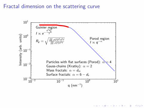
Fractal dimension on the scattering curve
10−2 10−1 100 101
q (nm−1)
10−3
10−2
10−1
100
101In
tensi
ty(a
rb.
unit
s)
Guinier region
I ∝ e−
q2R2g
3
I ∝ q−αRg =
√ tρ(~r)~r2d3~rtρ(~r)d3~r
Porod region
Particles with flat surfaces (Porod): α = 4Gauss-chains (Kratky): α = 2Mass fractals: α = dm
Surface fractals: α = 6 − ds

The pair density distribution function – back to the realspace
Electron
density
Inverse Fourier
transform
Fourier transform
AutocorrelationAbsolute
square
Scattered
amplitude
Differential
scattering c.s.
("intensity")
Distance
distribution
(PDDF)
There is another route connecting the electron density and thescattered intensity
The p(r) pair density distribution function (PDDF) is theself-correlation of the electron density.
p(r) = F−1 [I (q)] real space information. Physical meaning: find all the possible point pairs inside the particle
and make a histogram from their distances

The PDDFs of some geometrical shapes

Contents
IntroductionA bit of historyThe principle of scatteringSmall- and wide-angle scattering
BasicsScattering pattern and scattering curveScattering cross-sectionScattering variableScattering contrast
Basic relations of scatteringConnection between structure and scatteringPhase problemSpherically symmetric systemsThe Guinier ApproximationMulti-particle systems, size distributionPower-law scattering: the Porod regionThe pair density distribution function
Summary

Summary – Pros and cons of scattering experiments
Advantages
Statistically significant averageresults
Simple measurement principle
Separation of length scales(SAXS is blind for atomic sizes)
Accurate quantitative results,traceable to the definitions ofthe SI units of measurement
Disadvantages
Nonintuitive, indirectmeasurement results →difficult interpretation
Cannot be used on toocomplex systems
Possible ambiguity of thedetermined structure (phaseproblem)
Measures mean values: nomeans for getting results onstructural forms present inlow concentrations

Summary, outlook
Summary
Structure determination by scattering
Intensity, momentum transfer, scattering pattern, scattering curve
Fourier transform, absolute square, phase problem
Scattering of a homogeneous sphere, Guinier and Porod limits
Size distribution of nanoparticles
In the following weeks:
How to measure SAXS: instrumentation, practicalities
Different material systems: periodic samples, self-assembling lipidsystems (micelles, bilayers), proteins, polymer solutions, phaseseparated polymers: based on actual measurement data

Thank you for your attention!
Recommended