University of New Orleans University of New Orleans
ScholarWorks@UNO ScholarWorks@UNO
University of New Orleans Theses and Dissertations Dissertations and Theses
Fall 12-20-2013
Six Sigma, Firm Performance and Returns Predictability In Six Sigma, Firm Performance and Returns Predictability In
Emerging Real Estate Market Emerging Real Estate Market
Bora Ozkan University of New Orleans, [email protected]
Follow this and additional works at: https://scholarworks.uno.edu/td
Part of the Business Administration, Management, and Operations Commons, Corporate Finance
Commons, International Economics Commons, and the Real Estate Commons
Recommended Citation Recommended Citation Ozkan, Bora, "Six Sigma, Firm Performance and Returns Predictability In Emerging Real Estate Market" (2013). University of New Orleans Theses and Dissertations. 1756. https://scholarworks.uno.edu/td/1756
This Dissertation-Restricted is protected by copyright and/or related rights. It has been brought to you by ScholarWorks@UNO with permission from the rights-holder(s). You are free to use this Dissertation-Restricted in any way that is permitted by the copyright and related rights legislation that applies to your use. For other uses you need to obtain permission from the rights-holder(s) directly, unless additional rights are indicated by a Creative Commons license in the record and/or on the work itself. This Dissertation-Restricted has been accepted for inclusion in University of New Orleans Theses and Dissertations by an authorized administrator of ScholarWorks@UNO. For more information, please contact [email protected].

Six Sigma, Firm Performance and Returns Predictability in Emerging Real Estate Market
A Dissertation
Submitted to the Graduate Faculty of the University of New Orleans in partial fulfillment of the
requirements for the degree of
Doctor of Philosophy in
Financial Economics
by
Bora Ozkan
B.A. Hacettepe University, 2000 M.B.A. University of New Orleans, 2007
M.S. University of New Orleans, 2011
December 2013

ii
Dedication
To my mother, Prof. Dr. Olcay Ozkan for helping me become the person I am.
To my father, Nizamettin Ozkan for teaching me how to be strong even in tough times.
To my brother, Burak Ozkan for believing in me.
To Dr. Alan Bowers, for the unconditional support throughout the years.
To my dissertation advisors and all of my professors at the University of New Orleans, for being
instrumental in my career.
To my close friends, classmates and students for helping me dream big.

iii
Table of Contents
LIST OF TABLES .......................................................................................................................... iv
LIST OF FIGURES ......................................................................................................................... v
ABSTRACT .................................................................................................................................... vi
CHAPTER 1 .................................................................................................................................... 1
I. Motivation and Data ................................................................................................. 4
II. Literature Review ..................................................................................................... 5
III. Long run stock returns to investors in Six Sigma Firms ........................................... 7
A. Design................................................................................................................. 7
B. Results ................................................................................................................ 8
IV. Operating performance changes after Six Sigma .................................................... 11
A. Liquidity analysis ............................................................................................. 12
B. Activity analysis ............................................................................................... 12
C. Management efficiency .................................................................................... 13
D. Earnings ability (profitability) .......................................................................... 13
E. Labor (growth in staff levels and employee productivity) ............................... 13
F. Results .............................................................................................................. 14
V. Summary and conclusion ........................................................................................ 23
References ...................................................................................................................................... 24
CHAPTER 2 .................................................................................................................................. 27
I. Motivation .................................................................................................................. 28
II. Literature Review ....................................................................................................... 31
III. Data and Variables ..................................................................................................... 34
IV. Framework ................................................................................................................. 47
A. Predictability of Real Estate Price Index Returns ................................................ 47
A.1. Parameter Estimates ..................................................................................... 47
A.2. Forecasting Real Estate Price Index Returns ............................................... 48
B. Relationship among house prices, credit, money and economic activity ............ 52
B.1. Unit Root Test .............................................................................................. 52
B.2. Granger Causality Test ................................................................................. 53
B.3. Variance Decomposition .............................................................................. 56
V. Conclusion .............................................................................................................. 59
References ...................................................................................................................................... 60
Appendix A .................................................................................................................................... 64
Appendix B .................................................................................................................................... 65
Vita ................................................................................................................................................. 66

iv
LIST OF TABLES
CHAPTER 1
Table 1 – Long Run Abnormal Returns ......................................................................................... 10
Table 1 (Continued) ....................................................................................................................... 11
Table 2 – Operating Performance Measures .................................................................................. 16
Table 3 – Difference in mean test .................................................................................................. 17
Table 4 – Difference in mean test for Firms That Implemented Six Sigma Corporate-wide ........ 19
Table 5 – Difference in mean test for Firms That Implemented Six Sigma Before 2001 .............. 21
Table 6 - Difference in mean test for Firms That Implemented Six Sigma After 2000 ................. 22
CHAPTER 2
Table 1 – Summary Statistics......................................................................................................... 35
Table 2 – Fixed Effects Regression ............................................................................................... 47
Table 3 – Forecasting Real Estate Price Index .............................................................................. 49
Table 4 – Forecasting Real Estate Price Index for Different Regions ........................................... 51
Table 5 – Granger Causality Test .................................................................................................. 54
Table 5 (Continued) ....................................................................................................................... 55
Table 6 – Variance Decompositions .............................................................................................. 57
Table 6 (Continued) ....................................................................................................................... 58

v
LIST OF FIGURES
CHAPTER 2
Figure 1 – House Price Indices in Emerging Countries ................................................................. 36
Figure 1 (Continued) ...................................................................................................................... 37
Figure 1 (Continued) ...................................................................................................................... 38
Figure 2 – House Price and GDP Growth in Emerging Countries................................................. 41
Figure 2 (Continued) ...................................................................................................................... 42
Figure 2 (Continued) ...................................................................................................................... 43
Figure 3 – House Price and CPI Growth in Emerging Countries .................................................. 44
Figure 3 (Continued) ...................................................................................................................... 45
Figure 3 (Continued) ...................................................................................................................... 46

vi
Abstract
This dissertation consists of two essays. First essay investigates Fortune 500 companies
that implemented Six Sigma. Since the 1980s, industrial organizations have adopted practices
such as Six Sigma to maintain and enhance competitiveness. The purpose of this study is to look
at the long run stock price and the operating performance of Fortune 500 companies that were
identified to have implemented Six Sigma compared to the overall market performance as well
as the performance of industry and size matched firms. Even though our sample firms improved
several variables after implementing Six Sigma, their operating performances were not quite
close to the performances of the matching firms. After implementing Six Sigma, compared to the
industry and size matched firms, the only variable that improved out of 14 variables we looked
at, is the growth in staff levels. The findings may contribute to understanding the reasons that
underlie the so-called jobless recovery.
Second essay investigates the real estate price indices in 19 emerging markets. The main
objectives of the central banks are not necessarily in line with the goals for asset prices,
particularly house prices; however house price changes can have important implications for
economic activity and inflation. The consequences of excess changes in house prices also should
be watched carefully by central banks and other government agencies that regulate financial
institutions for the purpose of financial stability. This essay searches for a link between house
prices, broad money, private credit and the macro-economy among 19 emerging markets. We are
also trying to explain which variables predict the emerging markets real estate index returns. Our
results show that money market rate, growth in GDP and CPI as well as log of private credit and
money supply have significant predictive power on growth in real estate price indices a quarter
ahead. We also show that there is multidirectional causality among all of the variables. A unique

vii
data is being used for the emerging markets real estate price indexes in this study. The data is
provided by a Dubai based private company which offers emerging markets real estate
information to its customers.
Key Word: Six Sigma, Fortune 500, Abnormal Returns, Operating Performance, Growth in Staff,
Real Estate, Emerging Markets, Broad Money, Private Credit, Causality.

1
Chapter 1
Six Sigma, Stock Returns and Operating Performance
Managers are increasingly held accountable for delivering maximum shareholder value
while also providing improved relationships with stakeholders, particularly customers. Since the
1980s, industrial organizations have adopted practices such as Six Sigma to maintain and
enhance competitiveness. At once, the goals of these systematic programs are greater
satisfaction of customer needs and requirements as well as upgraded efficiency through lower
costs and enriched product quality. Realization of these goals would lead to larger profits and
higher shareholder wealth.
A major problem in most public corporations is the conflict of interest caused by the
separation of ownership and control, which is an “agency problem”. These agency problems lead
to frictions that reduce the value created by the corporation for its various stakeholders. The
conceptual idea of a Total Quality Management (TQM) philosophy is an extension of this
insight, actually. It is argued that “…agency frictions related to poor leadership, worker
alienation, and diminished morale account for the majority of productivity losses within
organizations. Moreover, most failures in organizations are caused by systemic flaws rather than
individual errors. Such flaws prevent companies from achieving levels of quality, or
productivity, that they might otherwise be capable of achieving.” (See W. Edwards Deming, The
New Economics, MIT Press, 1990.) Bacidore et al. (2005) discuss that “…TQM has
demonstrated that it has the potential to alter attitudes and behavior, improve motivation, and
reduce agency costs by eliciting the best efforts from all organizational stakeholders. These best

2
efforts can eliminate waste and enhance productivity significantly. ... The enhancement of
productivity from an effective TQM program should lead to lower costs, higher quality, and
increased market share, all of which ultimately result in greater shareholder wealth.”
In this paper, we also argue that Six Sigma may represent an attempt to communicate
about desirable organizational attributes to parties that cannot observe them directly. We argue
that Six Sigma may be an instrument to Managers for signaling quality to their customers.
Currently, one of the most popular quality programs is Six Sigma. The Six Sigma
approach, formulated by Motorola in the 1980s, is primarily a methodology for improving the
capability of business processes by using statistical methods to identify and decrease or eliminate
process variation. Its goal is reduction of defects and improvements in profits, employee morale
and product quality.
Motorola formulated Six Sigma in the 1980’s. The result was a total transformation of the
company by higher quality and lower costs. These results leaded Motorola to win the Malcolm
Baldrige National Quality Award in 1988 which brought great attention to Six Sigma among
major companies.
Six Sigma is simply an implementation of quality principles and methods at achieving
almost error-free business performance. Six Sigma capability is achieving merely 3.4 defects per
million outcomes. This process management goes beyond the oversight of the regular business
procedures to understanding business processes and flows of work. This understanding relies
heavily on documenting from the beginning to the end, from inputs to process activities and to
output. Customer expectations are clearly defined and updated on a regular basis. Therefore
actions are taken to address the problems and opportunities.

3
One important feature of Six Sigma is creating a structure to make sure that all the
necessary resources are provided to the performance improvement procedures. Before Six
Sigma, quality assurance was largely assigned to management on the production floor and to
some other technical people in a separate quality department. Six Sigma makes quality
improvement the job of a small but critical number of people who institutionalize change. This
infrastructure begins with the CEO and other top managers. Therefore Six Sigma is a top-down
implementation. Six Sigma creates a separate hierarchy in this structure, from Master Black Belt
to Black Belt and then to Green Belt. Master Black Belts provide leadership. Black Belts oversee
and support Green Belts and other improvement teams. Green Belt certification is usually
required. This certification may be obtained within the company itself or from outside providers
such as Villanova University which offers online certification courses. (Davis 2013)
Six Sigma project contains a five-step methodology called DMAIC. The first step is to
“define” the opportunity. This includes collecting any background information about the process
and defining the most important aspects for the customer. The next step is “measuring” the
process performance or collecting relevant data according to the parameters defined in step one.
Once the data is collected it can then be analyzed using statistical tools. The third step is
“Analyze” where the data is analyzed to determine gaps between the existing process and the
performance goals. The fourth step is to “improve” the solutions that were found after analyzing
the data. Finally the last step “controls” as a final check for the improvements that have been
implemented.
Quality is not obviously limited to manufacturers. Started at manufacturing companies,
Six Sigma, soon expanded to service and other industries. Hotels such as Ritz-Carlton are
examples. Quality is not even limited to businesses. Cities such as Madison, Wisconsin, and

4
counties such as Erie County, Pennsylvania, have been practicing quality methods. Under the
leadership of Admiral Frank B. Kelso, Chief of Naval Operations from 1990 to 1994, the U.S.
Navy committed to the practice of these same quality methods in it Total Quality Leadership
program. More recently, the U.S. Army Material Command has committed to “Lean Six Sigma”.
Which combines elements of lean manufacturing and Six Sigma. Morever, in 2007, the U.S.
Army Armament Research, Development and Engineering Center (ARDEC) won the Malcolm
Baldridge National Quality Award in the nonprofit category. (Davis, 2013)
Employee involvement is job training with focus on skills and knowledge to perform the
job. Companies that are committed to quality usually spend more than before on employee
training. In 1997, Citibank hired Motorola University Consulting and Training Services to teach
Six Sigma procedures to its employees. Citibank began its quality training initiative in 1997.
From May 1997 to October 1997, more than 650 senior managers were trained. Between
November 1997 and the end of 1998, another 7,500 employees attended sessions. By early 1999,
92,000 employees worldwide had been trained. Between 1996 and 1998, General Electric has
spent $1 billion on Six Sigma procedures. Since then thousands of companies world-wide started
implementing Six Sigma.
I. Motivation and Data
Over the past 20 years, use of Six Sigma has saved Fortune 500 companies an estimated
$427 billion, according to research published in the January/February 2007 issue of iSixSigma
Magazine. However, an increasing number of articles such as those in Fortune, The Wall St
Journal and Fast Company suggest that Six Sigma companies are failing. The market
performance of many companies like 3M, Ford, General Electric, Motorola, Delphi, Home

5
Depot, Larson, Eastman Kodak, and Xerox has fallen dramatically, and great number of Six
Sigma companies has trailed the S&P 500 since adopting Six Sigma.
The purpose of this study is to look at the long run stock price and the operating
performance of Fortune 500 companies that implemented Six Sigma process compared to the
overall market performance as well as the similar firms within their industries. We are using
2006 Fortune 500 companies so that we can compare up to 5 year after performance of these
companies. Companies usually implement Six Sigma at different levels; (1) Corporate, (2)
Business Unit, (3) Pilot and (4) Belt. (1) Corporate: Enterprise-wide initiative with corporate-
level executive support. (2) Business unit: Business unit deployment, supported by a corporate
executive and/or business unit general manager. (3) Pilot: Organized and supported pilot
initiative in one or more business units. The company is testing the water. (4) Belt: Unorganized
Black Belts and/or Green Belts. These may or may not be supported by executive or local
management. In 2006, 108 companies in the Fortune 500 were identified, with the initial start
date, as they had implemented Six Sigma. Of these 108 companies, eighty-five had implemented
Six Sigma at the corporate level, fourteen at the business unit level, four at the pilot level, and
five at the belt level.
II. Literature Review
Stock price reactions to the announcement of quality activities such as Malcolm Baldrige
National Quality Awards have been studied by Ramasesh (1998) and Przasnyski and Tai (1999).
Easton and Jarrell (1998) looks at the effects of TQM on corporate performance. Ramesesh
reports that the stock price movements around the day of the announcement increase the
shareholder wealth. Przasnyski and Tai show mixing results therefore recommend further

6
research. Easton and Jarrell, on the other hand, report long-term performance improvement of
firms that implemented TQM.
The impact of ISO 9000 certification on the performance of stock prices has been
analyzed by Docking and Dowen (1999) and Corbett, Montes-Sancho and Kirsh (2005). Long
run stock price performance was also analyzed by Ferreira, Sinha and Varble (2007). Docking
and Dowen show that for the smallest firms, ISO 9000 registration is regarded as positive
information by investors. Corbett, Montes-Sancho and Kirsh show that three years after
certification, the certified firms display significant abnormal returns. Ferreira, Sinha and Varble’s
results show that only stocks of large-size firms experience positive abnormal returns, whereas
stocks of mid-size firms experience negative average abnormal returns. Their results are not
consistent with the notion that companies that implement quality management system maybe
reducing agency cost.
Goh et al. (2003) investigated stock price reaction on the day when SixSigma activities
were made known publicly, as well as the long-run stock performance of ‘Six Sigma companies’
(sample of 20 firms) and found no significant abnormal returns.
Bacidore (1997) argue that Both TQM and EVA can be viewed as organizational
innovations designed to reduce “agency costs”. Terlaak and King (2006) investigate ISO 9000 as
a signaling approach. Their hypothesis is that certification may provide a way of communicating
about unobservable firm attributes, thereby generating a growth effect for certified organizations.
7
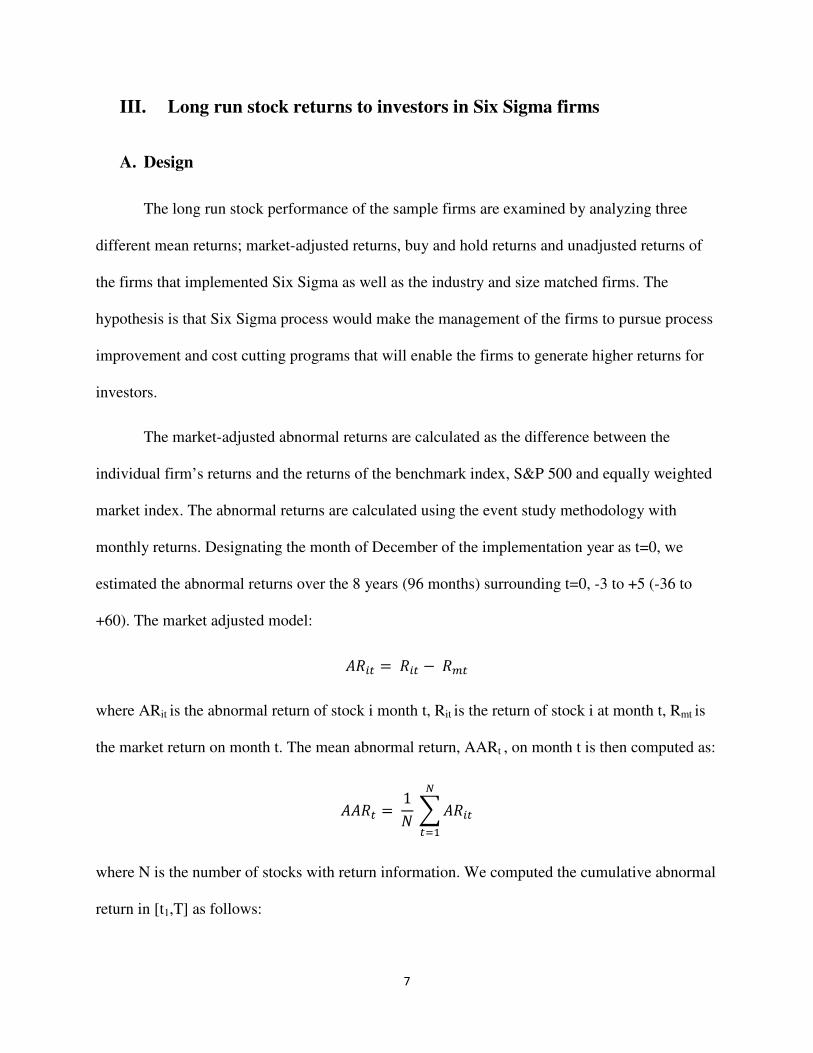
III. Long run stock returns to investors in Six Sigma firms
A. Design
The long run stock performance of the sample firms are examined by analyzing three
different mean returns; market-adjusted returns, buy and hold returns and unadjusted returns of
the firms that implemented Six Sigma as well as the industry and size matched firms. The
hypothesis is that Six Sigma process would make the management of the firms to pursue process
improvement and cost cutting programs that will enable the firms to generate higher returns for
investors.
The market-adjusted abnormal returns are calculated as the difference between the
individual firm’s returns and the returns of the benchmark index, S&P 500 and equally weighted
market index. The abnormal returns are calculated using the event study methodology with
monthly returns. Designating the month of December of the implementation year as t=0, we
estimated the abnormal returns over the 8 years (96 months) surrounding t=0, -3 to +5 (-36 to
+60). The market adjusted model:
���� � ��� � ���
where ARit is the abnormal return of stock i month t, Rit is the return of stock i at month t, Rmt is
the market return on month t. The mean abnormal return, AARt , on month t is then computed as:
���� � 1 � ����
�
� �
where N is the number of stocks with return information. We computed the cumulative abnormal
return in [t1,T] as follows:

8
����,� � � �����
� ��
The mean cumulative abnormal return is computed then as:
�����,� � 1 � � ����
�
� �
�
� ��
Then t-tests are conducted by dividing the abnormal returns by their contemporaneous cross-
sectional standard errors.
The buy and hold returns are the returns realized for buying the shares and holding them
for a period of -36, -24, -12, 12, 24, 36, 48 and 60 months. Following Byun and Rozeff (2003),
the buy and hold abnormal returns can be calculated as:
������ � ��1 � �����
� �� ��1 � ����
�
� �
where BHAR is the buy and hold abnormal returns, Ri is the returns for firm i, Rm is the returns
on the market index and n is the end of the holding period. The abnormal returns for each month
are obtained by taking the average across the sample. These returns are subsequently cumulated
over different periods over the 3 years before and 5 years after the Six Sigma implementation.
We conducted t-tests by dividing the abnormal returns by their contemporaneous cross-sectional
standard errors.
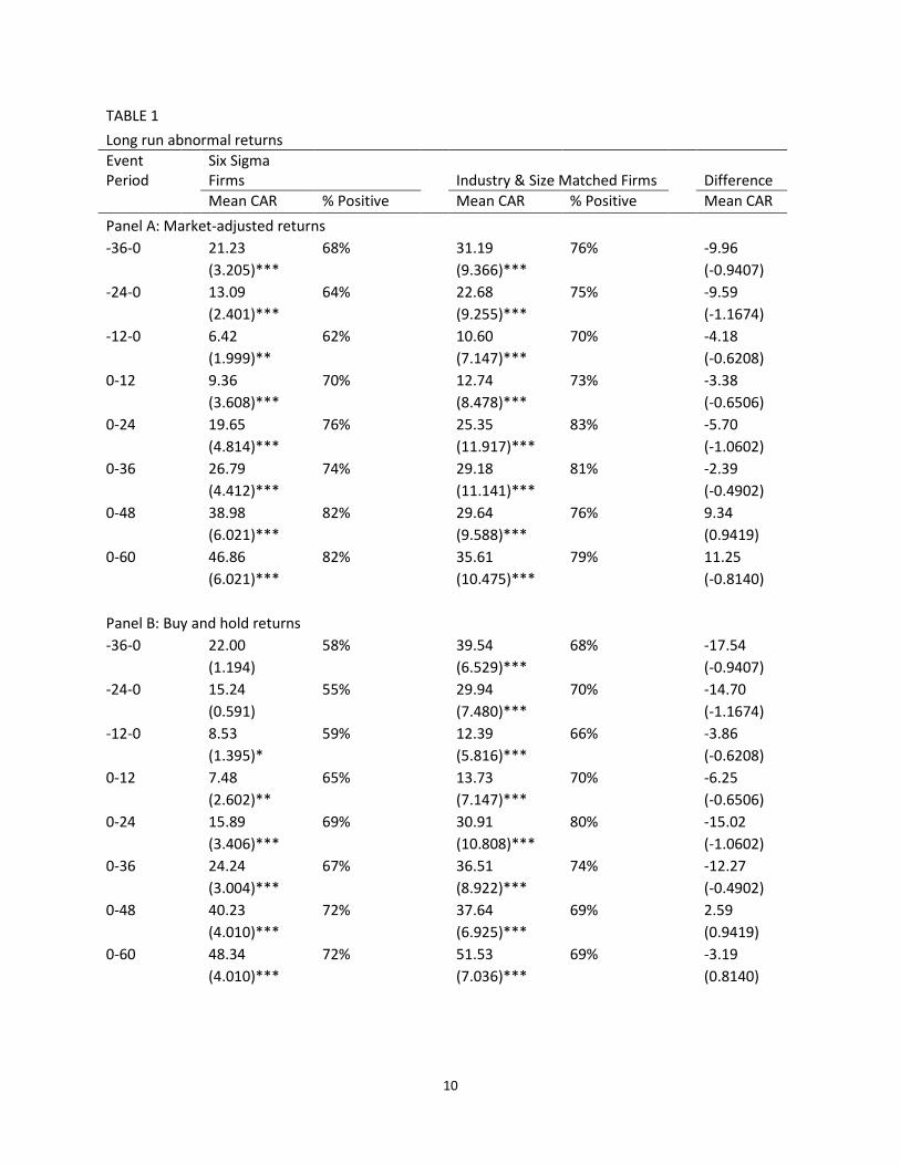
B. Results
The abnormal returns using the two returns are shown on Table 1. The market adjusted
returns for the firms that implemented Six Sigma and the industry and size matched firms are
shown in Panel A while the buy and hold returns are shown in Panel B. Panel C presents the

9
unadjusted returns. The results show that Six Sigma firms outperform the market both before and
after the Six Sigma implementation. We claim that managers use Six Sigma as a signal to
investor to show that they are committed to continued improvement of their process and efficient
use of the resources. Buy and hold abnormal returns are statistically significantly higher than the
S&P 500 and equally weighted indexes after implementing Six Sigma, 7.48% in one year and up
to cumulative return of 48.34% after five years. The abnormal returns become even more
significant at 1% level two years after implementation. The positive effects of Six Sigma on
abnormal returns start showing right after implementation, especially after three years. This may
also be an indicator of reduced agency cost as Six Sigma becomes more and more part of the
daily operations of companies.
When we compare these returns to the industry and size matched firms, the abnormal
returns are rather disappointing. Unadjusted mean cumulative abnormal returns from months -36
to 0 of matching firms are 57.35% compared to 50.81% of Six Sigma firms with a difference of
6.54%. The difference in return means keeps increasing each year which may indicate that the
firms are actually under pressure to implement Six Sigma as total quality management. Three
years after implementing Six Sigma, they finally start closing the gap with the matching firms
even though their abnormal returns are still lower even after five years.
If we look at the percentage of firms achieving positive mean cumulative abnormal
returns (CAR), the number increases as years go buy. While only 59% of our sample firms
achieved positive buy and hold CARs one year prior to implementing Six Sigma, 72% show
positive buy and hold CARs 5 years after.
10
TABLE 1
Long run abnormal returns
Event
Period
Six Sigma
Firms
Industry & Size Matched Firms
Difference
Mean CAR % Positive Mean CAR % Positive Mean CAR
Panel A: Market-adjusted returns
-36-0
21.23 68%
31.19 76%
-9.96
(3.205)***
(9.366)***
(-0.9407)
-24-0
13.09 64%
22.68 75%
-9.59
(2.401)***
(9.255)***
(-1.1674)
-12-0
6.42 62%
10.60 70%
-4.18
(1.999)**
(7.147)***
(-0.6208)
0-12
9.36 70%
12.74 73%
-3.38
(3.608)***
(8.478)***
(-0.6506)
0-24
19.65 76%
25.35 83%
-5.70
(4.814)***
(11.917)***
(-1.0602)
0-36
26.79 74%
29.18 81%
-2.39
(4.412)***
(11.141)***
(-0.4902)
0-48
38.98 82%
29.64 76%
9.34
(6.021)***
(9.588)***
(0.9419)
0-60
46.86 82%
35.61 79%
11.25
(6.021)***
(10.475)***
(-0.8140)
Panel B: Buy and hold returns
-36-0
22.00 58%
39.54 68%
-17.54
(1.194)
(6.529)***
(-0.9407)
-24-0
15.24 55%
29.94 70%
-14.70
(0.591)
(7.480)***
(-1.1674)
-12-0
8.53 59%
12.39 66%
-3.86
(1.395)*
(5.816)***
(-0.6208)
0-12
7.48 65%
13.73 70%
-6.25
(2.602)**
(7.147)***
(-0.6506)
0-24
15.89 69%
30.91 80%
-15.02
(3.406)***
(10.808)***
(-1.0602)
0-36
24.24 67%
36.51 74%
-12.27
(3.004)***
(8.922)***
(-0.4902)
0-48
40.23 72%
37.64 69%
2.59
(4.010)***
(6.925)***
(0.9419)
0-60
48.34 72%
51.53 69%
-3.19
(4.010)***
(7.036)***
(0.8140)
11
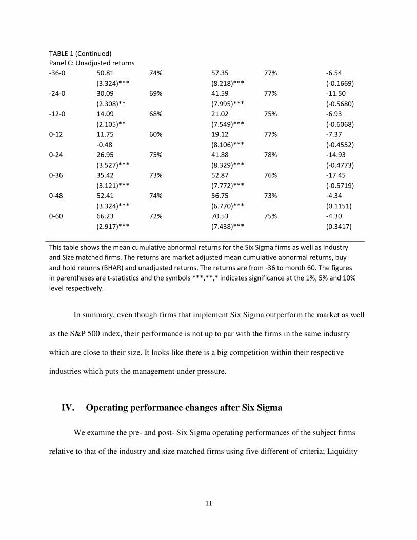
TABLE 1 (Continued)
Panel C: Unadjusted returns
-36-0
50.81 74%
57.35 77%
-6.54
(3.324)***
(8.218)***
(-0.1669)
-24-0
30.09 69%
41.59 77%
-11.50
(2.308)**
(7.995)***
(-0.5680)
-12-0
14.09 68%
21.02 75%
-6.93
(2.105)**
(7.549)***
(-0.6068)
0-12
11.75 60%
19.12 77%
-7.37
-0.48
(8.106)***
(-0.4552)
0-24
26.95 75%
41.88 78%
-14.93
(3.527)***
(8.329)***
(-0.4773)
0-36
35.42 73%
52.87 76%
-17.45
(3.121)***
(7.772)***
(-0.5719)
0-48
52.41 74%
56.75 73%
-4.34
(3.324)***
(6.770)***
(0.1151)
0-60
66.23 72%
70.53 75%
-4.30
(2.917)***
(7.438)***
(0.3417)
This table shows the mean cumulative abnormal returns for the Six Sigma firms as well as Industry
and Size matched firms. The returns are market adjusted mean cumulative abnormal returns, buy
and hold returns (BHAR) and unadjusted returns. The returns are from -36 to month 60. The figures
in parentheses are t-statistics and the symbols ***,**,* indicates significance at the 1%, 5% and 10%
level respectively.
In summary, even though firms that implement Six Sigma outperform the market as well
as the S&P 500 index, their performance is not up to par with the firms in the same industry
which are close to their size. It looks like there is a big competition within their respective
industries which puts the management under pressure.
IV. Operating performance changes after Six Sigma
We examine the pre- and post- Six Sigma operating performances of the subject firms
relative to that of the industry and size matched firms using five different of criteria; Liquidity
12
Analysis, Activity Analysis, Management Efficiency, Earnings Ability and Labor. We analyzed
14 ratios grouped under these five criteria. Details of the ratios are listed in Appendix A.
A. Liquidity analysis
Current ratio is a liquidity ratio that measures a company’s ability to pay short term
obligations. The higher the current ratio, the more capable the company is of paying its
obligations. A ratio under 1 suggests that the company would be unable to pay off its obligations
if they came due at that point. The quick ratio measures a company's ability to meet its short-
term obligations with its most liquid assets. The higher the quick ratio, the better the position of
the company. Net working capital is a measure of both a company's efficiency and its short-term
financial health.
B. Activity analysis
Activity analysis ratios are calculated to measure the efficiency with which the resources
of a firm have been employed. Asset turnover ratio measures a firm's efficiency at using its
assets in generating sales or revenue - the higher the number the better. Accounts receivable
turnover ratio is used to quantify a firm's effectiveness in extending credit as well as collecting
debts. The accounts receivable turnover ratio is an activity ratio, measuring how efficiently a
firm uses its assets. Inventory turnover ratio is a ratio showing how many times a company's
inventory is sold and replaced over a period. High inventory levels are unhealthy because they
represent an investment with a rate of return of zero. It also opens the company up to trouble
should prices begin to fall. Since Six Sigma is a process improvement, it is expected to improve
these ratios.

13
C. Management efficiency
We employed operating efficiency measures such as cost-to-income ratio and expense-to-
asset ratio as proxies for management efficiency. Lower ratios reflect higher management
efficiency. It is expected that because of greater emphasis on process improvement, the Six
Sigma firms would be more efficient than they were prior to the implementation of Six Sigma.
D. Earnings ability (profitability)
Six Sigma is expected to cut costs and improve defects. Therefore, we expect the
profitability of the Six Sigma firms to increase following their implementation of Six Sigma. We
use gross profit margin and return on assets (ROA) as measures of profitability. However, there
are several arguments that ROA is biased upwards. Consequently, we also employed return on
equity (ROE) as an alternative measure of profitability. Higher ratios indicate improvement in
performance.
E. Labor (growth in staff levels and employee productivity)
To ascertain whether a significant change in employment and labor productivity occurs
after implementing Six Sigma, we analyzed three labor-related ratios. First, we use the ratio of
asset-to-number of employees as a proxy for over-staffing and then analyze growth in staff levels
to ascertain whether the Six Sigma firms reduced staff levels after implementing Six Sigma.
Finally, we use the ratio of total revenue-to-number of employees to measure employee
productivity. We expect that Six Sigma firms will place more emphasis on cost cutting and are
therefore more likely to reduce employment and improve employee productivity after
implementing Six Sigma.
14
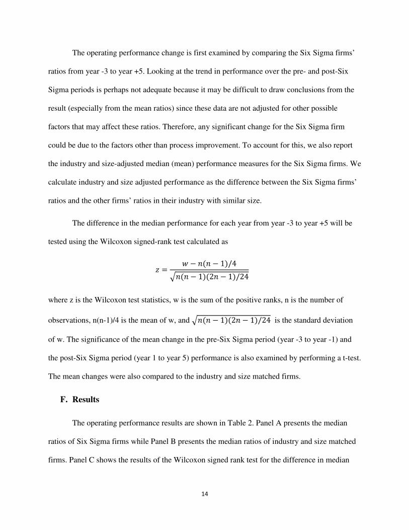
The operating performance change is first examined by comparing the Six Sigma firms’
ratios from year -3 to year +5. Looking at the trend in performance over the pre- and post-Six
Sigma periods is perhaps not adequate because it may be difficult to draw conclusions from the
result (especially from the mean ratios) since these data are not adjusted for other possible
factors that may affect these ratios. Therefore, any significant change for the Six Sigma firm
could be due to the factors other than process improvement. To account for this, we also report
the industry and size-adjusted median (mean) performance measures for the Six Sigma firms. We
calculate industry and size adjusted performance as the difference between the Six Sigma firms’
ratios and the other firms’ ratios in their industry with similar size.
The difference in the median performance for each year from year -3 to year +5 will be
tested using the Wilcoxon signed-rank test calculated as
� � � � ��� � 1�/4���� � 1��2� � 1�/24
where z is the Wilcoxon test statistics, w is the sum of the positive ranks, n is the number of
observations, n(n-1)/4 is the mean of w, and ���� � 1��2� � 1�/24 is the standard deviation
of w. The significance of the mean change in the pre-Six Sigma period (year -3 to year -1) and
the post-Six Sigma period (year 1 to year 5) performance is also examined by performing a t-test.
The mean changes were also compared to the industry and size matched firms.
F. Results
The operating performance results are shown in Table 2. Panel A presents the median
ratios of Six Sigma firms while Panel B presents the median ratios of industry and size matched
firms. Panel C shows the results of the Wilcoxon signed rank test for the difference in median
15
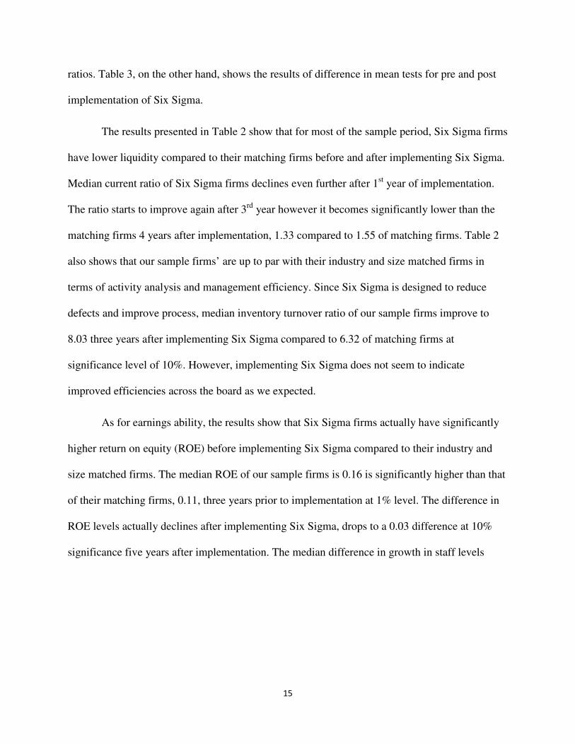
ratios. Table 3, on the other hand, shows the results of difference in mean tests for pre and post
implementation of Six Sigma.
The results presented in Table 2 show that for most of the sample period, Six Sigma firms
have lower liquidity compared to their matching firms before and after implementing Six Sigma.
Median current ratio of Six Sigma firms declines even further after 1st year of implementation.
The ratio starts to improve again after 3rd year however it becomes significantly lower than the
matching firms 4 years after implementation, 1.33 compared to 1.55 of matching firms. Table 2
also shows that our sample firms’ are up to par with their industry and size matched firms in
terms of activity analysis and management efficiency. Since Six Sigma is designed to reduce
defects and improve process, median inventory turnover ratio of our sample firms improve to
8.03 three years after implementing Six Sigma compared to 6.32 of matching firms at
significance level of 10%. However, implementing Six Sigma does not seem to indicate
improved efficiencies across the board as we expected.
As for earnings ability, the results show that Six Sigma firms actually have significantly
higher return on equity (ROE) before implementing Six Sigma compared to their industry and
size matched firms. The median ROE of our sample firms is 0.16 is significantly higher than that
of their matching firms, 0.11, three years prior to implementation at 1% level. The difference in
ROE levels actually declines after implementing Six Sigma, drops to a 0.03 difference at 10%
significance five years after implementation. The median difference in growth in staff levels
16
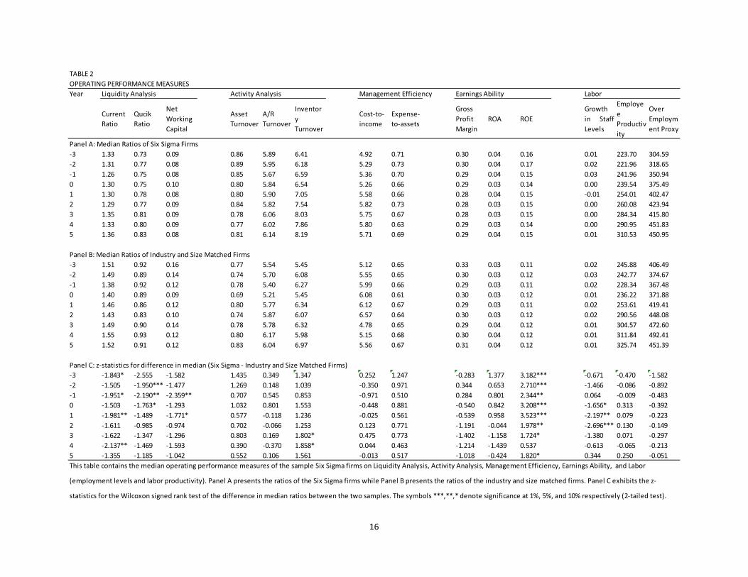
TABLE 2
OPERATING PERFORMANCE MEASURES
Year Liquidity Analysis Activity Analysis Management Efficiency Earnings Ability Labor
Current
Ratio
Qucik
Ratio
Net
Working
Capital
Asset
Turnover
A/R
Turnover
Inventor
y
Turnover
Cost-to-
income
Expense-
to-assets
Gross
Profit
Margin
ROA ROE
Growth
in Staff
Levels
Employe
e
Productiv
ity
Over
Employm
ent Proxy
Panel A: Median Ratios of Six Sigma Firms
-3 1.33 0.73 0.09 0.86 5.89 6.41 4.92 0.71 0.30 0.04 0.16 0.01 223.70 304.59
-2 1.31 0.77 0.08 0.89 5.95 6.18 5.29 0.73 0.30 0.04 0.17 0.02 221.96 318.65
-1 1.26 0.75 0.08 0.85 5.67 6.59 5.36 0.70 0.29 0.04 0.15 0.03 241.96 350.94
0 1.30 0.75 0.10 0.80 5.84 6.54 5.26 0.66 0.29 0.03 0.14 0.00 239.54 375.49
1 1.30 0.78 0.08 0.80 5.90 7.05 5.58 0.66 0.28 0.04 0.15 -0.01 254.01 402.47
2 1.29 0.77 0.09 0.84 5.82 7.54 5.82 0.73 0.28 0.03 0.15 0.00 260.08 423.94
3 1.35 0.81 0.09 0.78 6.06 8.03 5.75 0.67 0.28 0.03 0.15 0.00 284.34 415.80
4 1.33 0.80 0.09 0.77 6.02 7.86 5.80 0.63 0.29 0.03 0.14 0.00 290.95 451.83
5 1.36 0.83 0.08 0.81 6.14 8.19 5.71 0.69 0.29 0.04 0.15 0.01 310.53 450.95
Panel B: Median Ratios of Industry and Size Matched Firms
-3 1.51 0.92 0.16 0.77 5.54 5.45 5.12 0.65 0.33 0.03 0.11 0.02 245.88 406.49
-2 1.49 0.89 0.14 0.74 5.70 6.08 5.55 0.65 0.30 0.03 0.12 0.03 242.77 374.67
-1 1.38 0.92 0.12 0.78 5.40 6.27 5.99 0.66 0.29 0.03 0.11 0.02 228.34 367.48
0 1.40 0.89 0.09 0.69 5.21 5.45 6.08 0.61 0.30 0.03 0.12 0.01 236.22 371.88
1 1.46 0.86 0.12 0.80 5.77 6.34 6.12 0.67 0.29 0.03 0.11 0.02 253.61 419.41
2 1.43 0.83 0.10 0.74 5.87 6.07 6.57 0.64 0.30 0.03 0.12 0.02 290.56 448.08
3 1.49 0.90 0.14 0.78 5.78 6.32 4.78 0.65 0.29 0.04 0.12 0.01 304.57 472.60
4 1.55 0.93 0.12 0.80 6.17 5.98 5.15 0.68 0.30 0.04 0.12 0.01 311.84 492.41
5 1.52 0.91 0.12 0.83 6.04 6.97 5.56 0.67 0.31 0.04 0.12 0.01 325.74 451.39
Panel C: z-statistics for difference in median (Six Sigma - Industry and Size Matched Firms)
-3 -1.843* -2.555 -1.582 1.435 0.349 1.347 0.252 1.247 -0.283 1.377 3.182*** -0.671 -0.470 -1.582
-2 -1.505 -1.950*** -1.477 1.269 0.148 1.039 -0.350 0.971 0.344 0.653 2.710*** -1.466 -0.086 -0.892
-1 -1.951* -2.190** -2.359** 0.707 0.545 0.853 -0.971 0.510 0.284 0.801 2.344** 0.064 -0.009 -0.483
0 -1.503 -1.763* -1.293 1.032 0.801 1.553 -0.448 0.881 -0.540 0.842 3.208*** -1.656* 0.313 -0.392
1 -1.981** -1.489 -1.771* 0.577 -0.118 1.236 -0.025 0.561 -0.539 0.958 3.523*** -2.197** 0.079 -0.223
2 -1.611 -0.985 -0.974 0.702 -0.066 1.253 0.123 0.771 -1.191 -0.044 1.978** -2.696*** 0.130 -0.149
3 -1.622 -1.347 -1.296 0.803 0.169 1.802* 0.475 0.773 -1.402 -1.158 1.724* -1.380 0.071 -0.297
4 -2.137** -1.469 -1.593 0.390 -0.370 1.858* 0.044 0.463 -1.214 -1.439 0.537 -0.613 -0.065 -0.213
5 -1.355 -1.185 -1.042 0.552 0.106 1.561 -0.013 0.517 -1.018 -0.424 1.820* 0.344 0.250 -0.051
This table contains the median operating performance measures of the sample Six Sigma firms on Liquidity Analysis, Activity Analysis, Management Efficiency, Earnings Ability, and Labor
(employment levels and labor productivity). Panel A presents the ratios of the Six Sigma firms while Panel B presents the ratios of the industry and size matched firms. Panel C exhibits the z-
statistics for the Wilcoxon signed rank test of the difference in median ratios between the two samples. The symbols ***,**,* denote significance at 1%, 5%, and 10% respectively (2-tailed test).
17
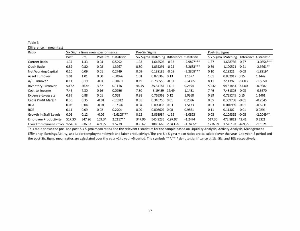
Table 3
Difference in mean test
Ratio Six Sigma firms mean performance Pre-Six Sigma Post-Six Sigma
Post Pre Post-Pre t-statistic Six Sigma Matching Difference t-statistic Six Sigma Matching Difference t-statistic
Current Ratio 1.37 1.33 0.04 0.5292 1.33 1.645506 -0.32 -2.9827*** 1.37 1.638786 -0.27 -3.0854***
Qucik Ratio 0.89 0.80 0.08 1.3767 0.80 1.055291 -0.25 -3.2683*** 0.89 1.100571 -0.21 -2.5661**
Net Working Capital 0.10 0.09 0.01 0.2749 0.09 0.138186 -0.05 -2.2308*** 0.10 0.13221 -0.03 -1.8319*
Asset Turnover 1.01 1.01 0.00 -0.0076 1.01 0.875365 0.13 1.1677 1.01 0.852917 0.15 1.1442
A/R Turnover 8.11 8.19 -0.08 -0.0461 8.19 8.758556 -0.57 -0.4335 8.11 22.1397 -14.03 -1.5550
Inventory Turnover 50.32 46.45 3.87 0.1116 46.45 35.34184 11.11 0.2494 50.32 94.31861 -44.00 -0.9287
Cost-to-income 7.46 7.30 0.16 0.0956 7.30 -5.19459 12.49 1.1451 7.46 7.481808 -0.03 -0.3670
Expense-to-assets 0.89 0.88 0.01 0.068 0.88 0.765368 0.12 1.0368 0.89 0.735245 0.15 1.1461
Gross Profit Margin 0.35 0.35 -0.01 -0.1912 0.35 0.345756 0.01 0.2086 0.35 0.359788 -0.01 -0.2545
ROA 0.03 0.04 -0.01 -0.7326 0.04 0.009833 0.03 1.5133 0.03 0.040989 -0.01 -0.5231
ROE 0.11 0.09 0.02 0.2704 0.09 0.008602 0.08 0.9861 0.11 0.11302 -0.01 0.0294
Growth in Staff Levels 0.03 0.12 -0.09 -2.6105*** 0.12 2.068984 -1.95 -1.0823 0.03 0.109365 -0.08 -2.2049**
Employee Productivity 517.30 347.96 169.34 2.2117** 347.96 545.9235 -197.97 -1.2474 517.30 473.8812 43.41 0.3321
Over Employment Proxy 1276.39 836.67 439.72 1.5279 836.67 1880.665 -1043.99 -1.7465* 1276.39 1776.182 -499.79 -1.1521
This table shows the pre- and post-Six Sigma mean ratios and the relevant t-statistics for the sample based on Liquidity Analysis, Activity Analysis, Management
Effiviency, Earnings Ability, and Labor (employment levels and labor productivity). The pre-Six Sigma mean ratios are calculated over the year -1 to year -3 period and
the post-Six Sigma mean ratios are calculated over the year +1 to year +5 period. The symbols ***,**,* denote significance at 1%, 5%, and 10% respectively.

18
starts to decline right after implementing Six Sigma. Two years after implementing, our sample
firms experience 0 growth rate while matching firms experience 0.02 and the difference in
growth in staff levels is statistically significant at 1% level.
When we look at the mean performances, as shown in Table 3, the only statistically
significant difference in performance measured before and after implementing Six Sigma are the
growth in staff levels and employee productivity. We find that Six Sigma firms’ post and pre
implementation difference in growth in staff levels is -0.09 at 1% significance level. Post-Six
Sigma mean employment productivity ratio of revenue to number of employees is 169.34 higher
than the pre-Six Sigma levels at 5%. This shows that while Six Sigma implementation reduces
the number of employees, it also increases employee productivity. However, when we compare
our sample firms with the matching firms both before and after implementing Six Sigma, we
cannot see statistically significant difference in performances except for the growth in staff levels
of -0.08 at 5%.
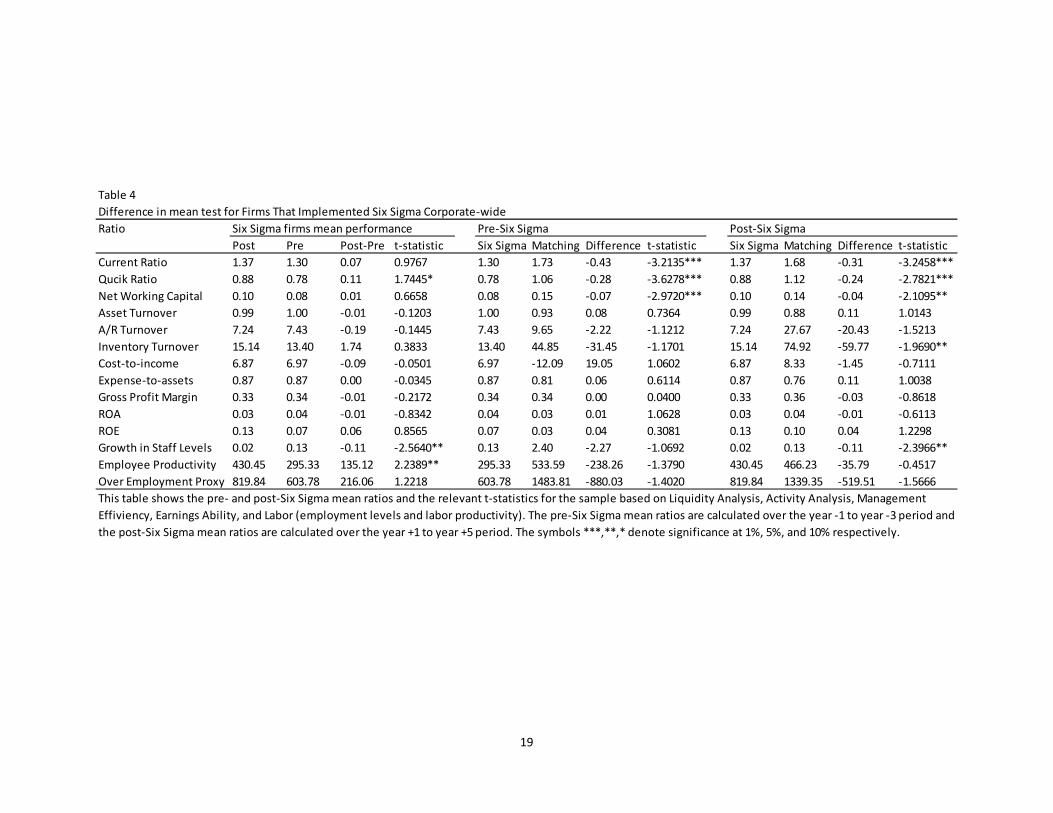
There are different types of implementing Six Sigma and the most common form is the
corporate wide implementation for our sample firms. Majority of our sample firms committed to
a corporate wide implementation as opposed to business unit, pilot or belts. We wanted to see if
we would see better improved performances if companies were more committed to Six Sigma
therefore conducted our mean tests on the smaller sample size of 85 firms that implemented Six
Sigma at corporate level.
19
Table 4
Difference in mean test for Firms That Implemented Six Sigma Corporate-wide
Ratio Six Sigma firms mean performance Pre-Six Sigma Post-Six Sigma
Post Pre Post-Pre t-statistic Six Sigma Matching Difference t-statistic Six Sigma Matching Difference t-statistic
Current Ratio 1.37 1.30 0.07 0.9767 1.30 1.73 -0.43 -3.2135*** 1.37 1.68 -0.31 -3.2458***
Qucik Ratio 0.88 0.78 0.11 1.7445* 0.78 1.06 -0.28 -3.6278*** 0.88 1.12 -0.24 -2.7821***
Net Working Capital 0.10 0.08 0.01 0.6658 0.08 0.15 -0.07 -2.9720*** 0.10 0.14 -0.04 -2.1095**
Asset Turnover 0.99 1.00 -0.01 -0.1203 1.00 0.93 0.08 0.7364 0.99 0.88 0.11 1.0143
A/R Turnover 7.24 7.43 -0.19 -0.1445 7.43 9.65 -2.22 -1.1212 7.24 27.67 -20.43 -1.5213
Inventory Turnover 15.14 13.40 1.74 0.3833 13.40 44.85 -31.45 -1.1701 15.14 74.92 -59.77 -1.9690**
Cost-to-income 6.87 6.97 -0.09 -0.0501 6.97 -12.09 19.05 1.0602 6.87 8.33 -1.45 -0.7111
Expense-to-assets 0.87 0.87 0.00 -0.0345 0.87 0.81 0.06 0.6114 0.87 0.76 0.11 1.0038
Gross Profit Margin 0.33 0.34 -0.01 -0.2172 0.34 0.34 0.00 0.0400 0.33 0.36 -0.03 -0.8618
ROA 0.03 0.04 -0.01 -0.8342 0.04 0.03 0.01 1.0628 0.03 0.04 -0.01 -0.6113
ROE 0.13 0.07 0.06 0.8565 0.07 0.03 0.04 0.3081 0.13 0.10 0.04 1.2298
Growth in Staff Levels 0.02 0.13 -0.11 -2.5640** 0.13 2.40 -2.27 -1.0692 0.02 0.13 -0.11 -2.3966**
Employee Productivity 430.45 295.33 135.12 2.2389** 295.33 533.59 -238.26 -1.3790 430.45 466.23 -35.79 -0.4517
Over Employment Proxy 819.84 603.78 216.06 1.2218 603.78 1483.81 -880.03 -1.4020 819.84 1339.35 -519.51 -1.5666
This table shows the pre- and post-Six Sigma mean ratios and the relevant t-statistics for the sample based on Liquidity Analysis, Activity Analysis, Management
Effiviency, Earnings Ability, and Labor (employment levels and labor productivity). The pre-Six Sigma mean ratios are calculated over the year -1 to year -3 period and
the post-Six Sigma mean ratios are calculated over the year +1 to year +5 period. The symbols ***,**,* denote significance at 1%, 5%, and 10% respectively.
20
Table 4 shows the mean performances of firms that implemented Six Sigma corporate-
wide compared to their industry and size matched firms. The results are quite similar to what we
found earlier. The quick ratio of these firms improved 0.11 however only at 10% significance
level. Growth in staff levels declined 0.11 while employee productivity increased 135.12. Pre
and post Six Sigma performances of this smaller sample firms compared to their industry and
size matched firms are similar to the larger sample except for the inventory turnover ratio. While
the mean inventory sample ratio of the larger sample, compared to the matching firms, did not
show any difference after implementing Six Sigma, the smaller sample indicated a 59.77
reduction in inventory level at 5% level post-Six Sigma.
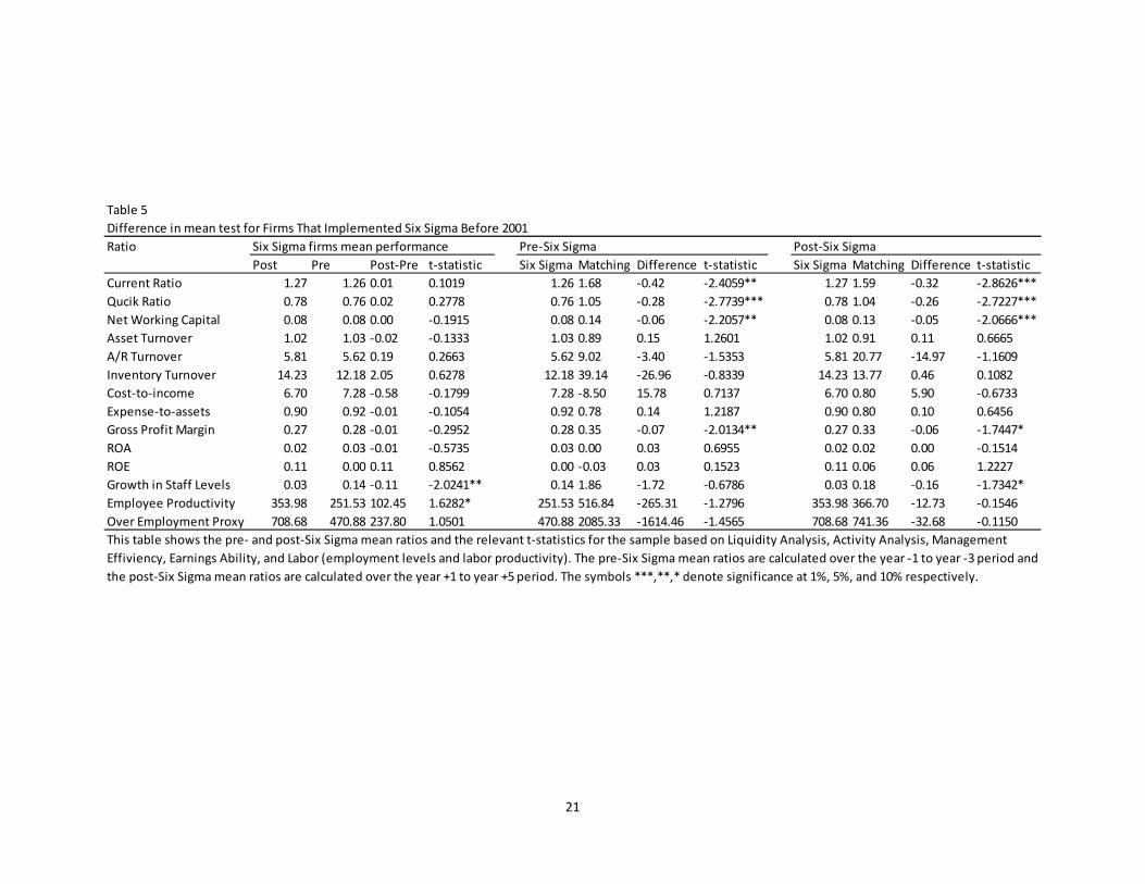
The earliest implementation of Six Sigma by our sample firms is 1987 however most
firms implemented in 1990’s and 2000’s. To account for early implementation and look for
advantages of early movers, we split our sample into two; firms that implemented Six Sigma
before 2001, and firms that implemented after 2000 since our median implementation is 2001.
Table 5 shows the mean results of early movers which implemented before 2001, while Table 6
shoes the mean results of the later implementers.
Based on results shown in Table 5, we see that the mean gross profit margin of the firms
that implemented Six Sigma is actually 0.07 lower than that industry and size matched firms
prior to Six Sigma. This ratio gap only declines to 0.01 and becomes -0.06 difference after Six
Sigma at 10% significance level. This is an indicator that the billions of dollars of savings that
these firms claim they experienced after implementing Six Sigma, does not reflect to their
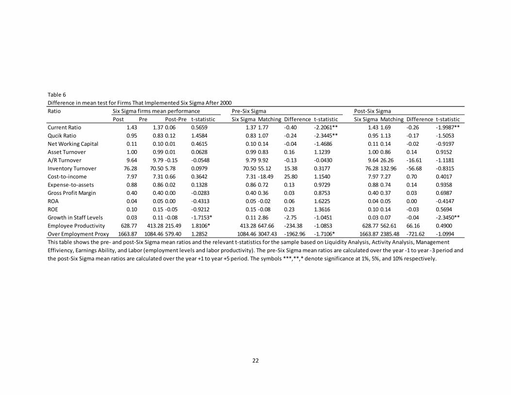
bottom-line; profit margins. When we look at the later implementers in Table 6, the results are
quite similar to the overall performances of these firms.
21
Table 5
Difference in mean test for Firms That Implemented Six Sigma Before 2001
Ratio Six Sigma firms mean performance Pre-Six Sigma Post-Six Sigma
Post Pre Post-Pre t-statistic Six Sigma Matching Difference t-statistic Six Sigma Matching Difference t-statistic
Current Ratio 1.27 1.26 0.01 0.1019 1.26 1.68 -0.42 -2.4059** 1.27 1.59 -0.32 -2.8626***
Qucik Ratio 0.78 0.76 0.02 0.2778 0.76 1.05 -0.28 -2.7739*** 0.78 1.04 -0.26 -2.7227***
Net Working Capital 0.08 0.08 0.00 -0.1915 0.08 0.14 -0.06 -2.2057** 0.08 0.13 -0.05 -2.0666***
Asset Turnover 1.02 1.03 -0.02 -0.1333 1.03 0.89 0.15 1.2601 1.02 0.91 0.11 0.6665
A/R Turnover 5.81 5.62 0.19 0.2663 5.62 9.02 -3.40 -1.5353 5.81 20.77 -14.97 -1.1609
Inventory Turnover 14.23 12.18 2.05 0.6278 12.18 39.14 -26.96 -0.8339 14.23 13.77 0.46 0.1082
Cost-to-income 6.70 7.28 -0.58 -0.1799 7.28 -8.50 15.78 0.7137 6.70 0.80 5.90 -0.6733
Expense-to-assets 0.90 0.92 -0.01 -0.1054 0.92 0.78 0.14 1.2187 0.90 0.80 0.10 0.6456
Gross Profit Margin 0.27 0.28 -0.01 -0.2952 0.28 0.35 -0.07 -2.0134** 0.27 0.33 -0.06 -1.7447*
ROA 0.02 0.03 -0.01 -0.5735 0.03 0.00 0.03 0.6955 0.02 0.02 0.00 -0.1514
ROE 0.11 0.00 0.11 0.8562 0.00 -0.03 0.03 0.1523 0.11 0.06 0.06 1.2227
Growth in Staff Levels 0.03 0.14 -0.11 -2.0241** 0.14 1.86 -1.72 -0.6786 0.03 0.18 -0.16 -1.7342*
Employee Productivity 353.98 251.53 102.45 1.6282* 251.53 516.84 -265.31 -1.2796 353.98 366.70 -12.73 -0.1546
Over Employment Proxy 708.68 470.88 237.80 1.0501 470.88 2085.33 -1614.46 -1.4565 708.68 741.36 -32.68 -0.1150
This table shows the pre- and post-Six Sigma mean ratios and the relevant t-statistics for the sample based on Liquidity Analysis, Activity Analysis, Management
Effiviency, Earnings Ability, and Labor (employment levels and labor productivity). The pre-Six Sigma mean ratios are calculated over the year -1 to year -3 period and
the post-Six Sigma mean ratios are calculated over the year +1 to year +5 period. The symbols ***,**,* denote significance at 1%, 5%, and 10% respectively.
22
Table 6
Difference in mean test for Firms That Implemented Six Sigma After 2000
Ratio Six Sigma firms mean performance Pre-Six Sigma Post-Six Sigma
Post Pre Post-Pre t-statistic Six Sigma Matching Difference t-statistic Six Sigma Matching Difference t-statistic
Current Ratio 1.43 1.37 0.06 0.5659 1.37 1.77 -0.40 -2.2061** 1.43 1.69 -0.26 -1.9987**
Qucik Ratio 0.95 0.83 0.12 1.4584 0.83 1.07 -0.24 -2.3445** 0.95 1.13 -0.17 -1.5053
Net Working Capital 0.11 0.10 0.01 0.4615 0.10 0.14 -0.04 -1.4686 0.11 0.14 -0.02 -0.9197
Asset Turnover 1.00 0.99 0.01 0.0628 0.99 0.83 0.16 1.1239 1.00 0.86 0.14 0.9152
A/R Turnover 9.64 9.79 -0.15 -0.0548 9.79 9.92 -0.13 -0.0430 9.64 26.26 -16.61 -1.1181
Inventory Turnover 76.28 70.50 5.78 0.0979 70.50 55.12 15.38 0.3177 76.28 132.96 -56.68 -0.8315
Cost-to-income 7.97 7.31 0.66 0.3642 7.31 -18.49 25.80 1.1540 7.97 7.27 0.70 0.4017
Expense-to-assets 0.88 0.86 0.02 0.1328 0.86 0.72 0.13 0.9729 0.88 0.74 0.14 0.9358
Gross Profit Margin 0.40 0.40 0.00 -0.0283 0.40 0.36 0.03 0.8753 0.40 0.37 0.03 0.6987
ROA 0.04 0.05 0.00 -0.4313 0.05 -0.02 0.06 1.6225 0.04 0.05 0.00 -0.4147
ROE 0.10 0.15 -0.05 -0.9212 0.15 -0.08 0.23 1.3616 0.10 0.14 -0.03 0.5694
Growth in Staff Levels 0.03 0.11 -0.08 -1.7153* 0.11 2.86 -2.75 -1.0451 0.03 0.07 -0.04 -2.3450**
Employee Productivity 628.77 413.28 215.49 1.8106* 413.28 647.66 -234.38 -1.0853 628.77 562.61 66.16 0.4900
Over Employment Proxy 1663.87 1084.46 579.40 1.2852 1084.46 3047.43 -1962.96 -1.7106* 1663.87 2385.48 -721.62 -1.0994
This table shows the pre- and post-Six Sigma mean ratios and the relevant t-statistics for the sample based on Liquidity Analysis, Activity Analysis, Management
Effiviency, Earnings Ability, and Labor (employment levels and labor productivity). The pre-Six Sigma mean ratios are calculated over the year -1 to year -3 period and
the post-Six Sigma mean ratios are calculated over the year +1 to year +5 period. The symbols ***,**,* denote significance at 1%, 5%, and 10% respectively.

23
V. Summary and conclusion
In this paper, we present a comprehensive analysis of the pre- and post-Six Sigma
performances of Fortune 500 firms that implemented Six Sigma as Total Quality Management
(TQM) initiative. We argue that managers may be implementing TQM to signal to investors their
commitment to improved efficiency and bottom-line. We also argue that these programs reduce
the agency costs by improving efficiency.
First, we analyzed the market adjusted as well as buy-and-hold abnormal returns to see if
firms that implement Six Sigma under-performed or over-performed the market. Our findings
show that firms that implemented Six Sigma outperformed the market as well as the S&P 500
index; however their performance is not up to par with the firms within the same industry which
are close to their size. This may be due to a big competition within their respective industries
which puts the management under pressure.
Second, we investigated the improvements in the operating performance of the firms that
implement Six Sigma by looking at 14 ratios grouped under five criteria; liquidity, activity,
management, earnings ability, labor. We had expected that the firms which implement Six Sigma
would show improved results and better performance compared to their industry and size
matching firms, however due to a possible high training costs as well as high opportunity costs
our results show some conflicting results which may have important implications for the firms as
well as their investors.
Even though our sample firms improved several variables after implementing Six Sigma,
they were not quite close to the performances of matching firms. After implementing Six Sigma,
compared to the industry and size matched firms, the only variable that improves out of 14
24
variables we looked at, is the growth in staff levels. The Six Sigma phenomenon may be one of
the reasons behind “jobless recovery” economists have been discussing recent years.
We conclude that implementing Six Sigma may reduce agency cost in the long run and
help the firms catch-up with the level of abnormal returns their industry and size matched piers
are achieving. It also looks like managers may be using Six Sigma as a signaling tool to commit
to their customers as well as investors for better quality goods and services. Investors seem to
believe in this commitment in the long run since even though operating performances do not
show significant difference after implementing Six Sigma, abnormal returns keeps increasing.
References
• Akhigbe, A., Madura, J., 1999. The industry effects regarding the probability of
takeovers, The Financial Review 34, 1–18.
• Bacidore, JM, Boquist, JA, Milbourn, TT, Thakor, A., 1997. EVA and total quality
management, Journal of Applied Corporate Finance, Volume 10, Issue 2, pages 81–89
• Chen and Wang, Applying Lean Six Sigma and TRIZ methodology in banking services,
Total Quality Management Vol. 21, No. 3, March 2010, 301–315
• Corbett, C. J., Montes-Sancho, M., and Kirsch, D., 2005, The Financial Impact of ISO
9000 Certification in the United States: An Empirical Analysis, Management Science.
• Cornett, M.M., Tehranian, H., 1990. An examination of the impact of the Garn-St
Germain Depository Institutions Act of 1982 on commercial banks and savings and
loans, Journal of Finance 45, 95–111.
• Dowen, R. and Docking, D.S., 1998, Market interpretation of ISO 9000 registration,
Journal of Financial Research

25
• Easten and Tarrell, The Effects of Total Quality Management on Corporate Performance:
An Empirical Investigation, The Journal of Business, Vol. 71, No. 2 (April 1998), pp.
253-307
• Ferreira, E., Sinha, A., and Varble, D., 2008, Long-run performance following quality
management certification, Review of Quantitative Finance and Accounting
• Firth, M., 1996. Dividend changes, abnormal returns, and intra-industry firm valuations,
Journal of Financial and Quantitative Analysis 31, 189–210.
• Goh, T.N., Low, P.C., Tsui, K.L. and Xie, M.: Impact of Six Sigma implementation on
stock price performance, TQM & Business Excellence, Vol. 14, No. 7, September, 2003,
753–763
• King and Terlaag, The Effect Of Certification With The Iso 9000 Quality Management
Standard: A Signaling Approach, Journal of Economic Behavior and Organization,
• Kaynak, The relationship between total quality management practices and their effects on
firm performance, Journal of Operations Management 21 (2003) 405–435
• Laux, P., Stark, L., Yoon, S.Y., 1998. The relative importance of competitive and
contagion intra-industry information transfers: An investigation of dividend
announcements, Financial Management 27, 5–16.
• Otchere, Do privatized banks in middle- and low-income countries perform better than
rival banks? An intra-industry analysis of bank privatization, Journal of Banking &
Finance (2005)
• Persons, O.S., 1999. Using financial information to differentiate failed vs. surviving
finance companies in Thailand: An application for emerging economies. Multinational
Finance Journal 3, 127–145.

26
• Powel, 1995, Total Quality Management as Competitive Advantage: A Review and
Empirical study, Strategic Management Journal.
• Przasnyski, Z. and Tai, L., 1999, Stock Market reaction to Malcolm Baldridge National
Quality Award announcements: does quality pay?, Total Quality Management
• Ramasasesh, R., 1998, Baldrige Award announcement and shareholder wealth,
International Journal of Quality Science, Vol. 3 Iss:2, pp. 114-125
• Slovin, M., Sushka, M., Bendeck, Y., 1991. The intra-industry effects of going-private
transactions, Journal of Finance 46, 1537–1550.
• Szewczyck, S., 1992. The intra-industry transfer of information inferred from
announcements of corporate security offerings, Journal of Business (July), 1935–1945.
• Thomson, J.B., 1991. Predicting bank failure in the 1980s. Economic Review – Federal
Reserve Bank of Cleveland (1st quarter), 9–20.

27
Chapter 2
Returns Predictability in Emerging Real Estate Market
Since the collapse of the US subprime market in 2007, much attention has been given to
the linkage between real estate markets and the macroeconomic variables as well as financial
markets in developed countries. Several studies showed that real estate markets and stock
markets are integrated (Lin and Lin, 2011; Liow and Webb, 2009) and macroeconomic variables
also have effects on these markets (Kishor, 2007; Aizenman and Jinjarak, 2009; Miller, Peng and
Sklarz, 2009). Investments to real estate, however, has a major disadvantage; liquidity. Despite
of the several disadvantages, investments to securitized real estate have been increasing
exponentially. According to Brounen et al. (2006) the market capitalization for securitized real
estate was at USD 800 billion level by the end of 2005. There are several types of securitized
real estate available out there such as closed and open-end funds, listed real estate companies,
REIT’s or real estate private equity companies.
Property price fluctuations has played a role in past business cycles, stimulating the
upswing and increasing the downswing. On the other hand, business cycles cause property price
fluctuations as well. Improvements in overall economic conditions tend to increase the income of
households and therefore boost the demand for new homes which puts an upward pressure on
house prices. The movements of real estate prices and the extent to which they interact with the
financial sector and the macro-economy have been given attention by the monetary authorities
and financial regulators.
Macroeconomic theory suggests that money serves as a proxy for the substitution effect
of the monetary policy since asset prices matter for aggregate demand. On one hand an

28
expansion of money supply influences both the mean and the dynamics of inflation (Nelson,
2003). On the other hand not only house prices influence monetary developments, relationship
can be both ways; there is a strong link from liquidity to the real estate market in the US and
Euro area (Greiber and Setzer, 2007).
For industrialized countries, Goodhart and Hofmann (2008) show a significant
multidirectional link between house prices, broad money, private credit and the macro-economy.
Their results show that money growth has a significant effect on house prices and private credit,
private credit effects money as well as house prices and finally house prices influence both
private credit and money. The study of Greiber and Setzer (2007) also shows strong evidence
that monetary policy influences housing market developments by improving financing
conditions, thereby increasing demand for housing for the US and Euro area. Emerging markets,
on the other hand, can have different dynamics therefore we may not expect the same results as
in the industrialized countries.
Our main objective is to investigate the interrelationship between the emerging markets
real estate index returns and broad money, private credit and the macro-economy among 19
emerging markets. To our knowledge, no research has been conducted on emerging markets real
estate price indices, and money, credit and macro variables on a broad level.
I. Motivation
Just like any other security, real estate investment also has its risks including falling
property values, lack of liquidity, limited diversification and sensitivity to certain economic and
financial factors. The question we are looking for is if there is evidence of a significant link
among house price indices, money, credit and the macro economy. Goodhart (2007) argue that

29
modern-style macro models are inherently non-monetary. He claims “…Since there are by
construction no banks, no borrowing constraints and no risks of default, the risk free short-term
interest rate serves to model the monetary side of the economy. As a consequence, money or
credit aggregates and asset prices play no role in standard versions of these models.”
Interest rates have direct effects on house prices. House prices appear to be associated
with business-cycle movements in a number of real variables, such as consumption and
investment. Researches have not fully agreed on as to whether accommodative policy has
contributed to the volatility of house or other asset prices. It can be argued that because house
prices, macroeconomic and monetary variables move in response to other outside shocks hitting
the economy, the direction of the relationship or the extent of causality among these variables
can be difficult to point out.
The main objectives of the central banks are not necessarily in line with the goals for
asset prices, particularly house prices; however house price changes can have important
implications for economic activity and inflation. This effect has become especially more
important since 2008 crisis. The consequences of excess changes in house prices also should be
watched carefully by central banks and other government agencies that regulate financial
institutions for the purpose of financial stability. Even though in the past, major declines in real
house prices have often been associated with economic downturns, 2008 crises showed us that
the opposite is also true; economic downturn can be caused by a decline in real house prices,
especially when collateral values also decline significantly.
There is not a consensus among central banks as to how to react to excess changes in
house prices. Some researchers argue that we should trust the markets therefore central banks
should continue focusing on their goal of low inflation and output stability. However, there are

30
also several researchers who claim central banks should act to prevent bubbles in real estate
prices to avoid financial as well as macroeconomic turbulences. The question is then how should
central banks respond to movements in asset prices? There is also not a consensus on this
question. Some researches advise that the price index targeted by a central bank should also
include the future prices of goods and services as well as assets. Some researchers, on the other
hand, argue that as long as the asset prices affect the forecast of future goods and services price
inflation, they can be subject to the monetary policy. They claim central banks should respond to
changes in asset prices by calculating the effect of the change in asset prices on expected
inflation, and then adjusting the interest rates. Several researchers also point out that the changes
in asset prices have implications for the stability of the financial sector; therefore there is an
indirect relationship with monetary policy as well. If there is a bubble in asset prices, a correction
might be inevitable. When the correction occurs it can be very costly to financial institutions
therefore can impair the financial stability. It is clear that understanding the sources of asset price
movements becomes a key element in determining the necessary monetary policy response.
Hence, movements of real estate prices and the how these movements effect the financial sector
and the macro-economy should closely be monitored by monetary authorities and financial
regulators.
Using the fixed effects panel data approach, we analyze the variation in 19 emerging
markets real estate index returns. The results show that money market rate as well as growth in
GDP, Consumer Price Index, private credit and money supply have significant predictive power
on growth in real estate price indices a quarter ahead. Using Vector Autoregression Model
(VAR) methodology, the findings are expected to contribute to the evaluation of the emerging

31
markets real estate price index behavior taking into consideration of several financial and
economic factors.
Granger Causality tests reveal strong evidence of multi-directional causality between
house prices, GDP, CPI, interest rates, money, and credit. In almost every country we
investigated, forecast errors to GDP, CPI and money market rate play an important role in
explaining innovations to the real estate price index returns.
The rest of the study is outlined as follows. Section 2 conducts a literature review.
Section 3 explains the data as well as the variables used. Section 4 outlines the framework of the
methodology used in this study. Section 5 presents the conclusion of the study.
II. Literature Review
The academic studies primarily focus on the link between the housing sector and its
economy. Using a vector autoregressive (VAR) model Baffoe-Bonnie (1998) tries explain the
relationship between house prices and macroeconomic key aggregates in US sub-regions. He
finds that variables influence very differently across these sub-regions. Kasparova and White
(2001) examine the housing markets in selected European countries using VECM. They show
that effect of house prices on GDP is significantly greater than the effect of GDP on house
prices. Tsatsaronis and Zhu (2004) investigate the impact of GDP, inflation and the interest rates
over house prices. They show that the main reason behind the changes in house prices is the
inflation hedge characteristics of residential real estate. They also show that the importance of
interest rates became more obvious in the last decade of their study.
In a Federal Reserve Bank International Finance Discussion Paper (2005), Aherane et al.
found that in 18 major industrial countries real house prices are pro-cyclical and they move

32
together with real GDP, consumption, investment, CPI inflation, budget and current account
balances, and output gaps. They show that house price booms are preceded by a period of easing
monetary policy. After a period of rising inflation, monetary authorities begin to tighten policies
before house prices peak.
Goodhart and Hoffman (2008) show that there is evidence of a significant
multidirectional link between house prices, broad money, private credit and the macro economy
among 17 industrialized countries. Their main results reveal that there is evidence of a
significant multidirectional link between house prices, monetary variables and the macro-
economy. They also results suggest that the link between housing prices and monetary variables
is stronger over more recent years and that the effects of shocks to money and credit are stronger
when housing prices are booming. In a more recent study, Beltratti and Morana (2010) suggested
countries that macroeconomic variables, such as interest rates and monetary aggregates, affect
housing prices in G7 countries.
Asset-price volatility is believed to have been critical effected by the macro-economy.
(Gilchrist and Leahy, 2002). Several research show that the housing market has a significant
connection with the performance of the overall economy and with monetary policy (Darrat and
Glascock, 1989; Ball, 1994; Baffoe-Bonnie, 1998; Lastrapes, 2002; Jin and Zeng, 2004,
Goodhart and Hofmann, 2008). Darrat and Glascock (1989) examined the causal relationship
between money supply and real estate return and found that money supply plays an important
role in changes in real estate return. Breedon and Joyce (1992) added gross financial wealth into
their housing price model. They claim that money supply has a lagged effect on current real
estate returns, implying a possible rejection of market efficiency. More recent studies have
discussed how the relationship between money supply and asset investment leads to strong

33
housing price fluctuation. Lastrapes (2002) used VAR model to estimate the dynamic response
of housing prices to money supply shocks and interpreted these responses based on the asset
view of housing demand. Jin and Zeng (2004) found that monetary policy and nominal interest
rates play a significant role in the determination of housing prices, as do money shocks by
generating remarkably volatile residential investment.
Kim (2005) looked at differential effects of monetary policy on housing sub-markets,
specifically new home construction and existing home sales. Findings show that the existing
home sale market is relatively more affected by expansionary monetary policies than is the new
home construction market in the short run.
McCue and Kling (1994) examine the relationship between US equity REIT series
returns and a set of macroeconomic variables. The findings indicate that nearly 60% of the
variation in real estate prices is explained by the macro economy; thereby it is the nominal short-
term interest rate variable that explains the majority of the real estate price movement. In a more
recent study by Ewing and Payne (2005), it is found that shocks to monetary policy, economic
growth, and inflation have negative impact on expected REIT returns, while on the other hand
shocks to the default risk premium have positive impact on future expected returns.
Mei and Lee (1994) found the presence of a real estate factor, in addition to both a stock
factor and a bond factor in asset pricing. They suggest that mutual fund managers should
consider including real estate assets in their portfolios.
Gyourko and Keim (1992) found evidence that REIT returns in the US stock market
predict returns to un-securitized returns to commercial properties. They concluded that the prior
year's REIT return is significant in predicting the current year's un-securitized real estate return.
Myer and Webb (1993) also analyzed the lead-lag relationship using Granger causality. Their

34
findings show that equity REITs Granger cause un-securitized real estate returns. Quan and
Titman (1999) prove that real estate is positively affected by inflation as well as GDP.
Ray and Vani (2003) prove that interest rates, industrial production, money supply,
inflation and exchange rates have significant affect over equity prices. Hoesli et al. (2008)
present the inflation characteristics of real estate investment in the United Kingdom as well as
the United States. They show a positive relationship between commercial real estate returns and
expected inflation in both countries.
Schatz and Sebastian (2009) find a positive linkage between the property markets and
consumer prices as well as the government bonds, while the property markets are negatively
affected by the respective unemployment rates for Germany and the UK. Schatz, in his second
essay, study on the issue of whether real estate stock indices are primarily driven by the progress
of property markets or by developments on general stock markets for the US and the UK. He
shows that the real estate equity markets are predominantly driven by the underlying properties.
III. Data and Variables
Emerging markets Real Estate Price Index data for 19 Emerging Markets (see Appendix
A.) provided by Reidin.com; Bulgaria, Czech Republic, Estonia, Hong Kong Sar, Hungary,
Israel, Indonesia, Lithuania, Latvia, Mexico, Malaysia, Poland, Romania, Russia, Slovenia,
Slovak Republic, South Africa, South Korea, Thailand, and Turkey. The sample period ranges
from 1966Q1 to 2012Q2 which makes an unbalanced panel data set with a total of 906 quarters.
On average there are 47 quarters per country; South Africa has the longest sample period with
186 quarters, whereas Thailand has the shortest with 18 quarters. The details of each country
period is provided in the Appendix.
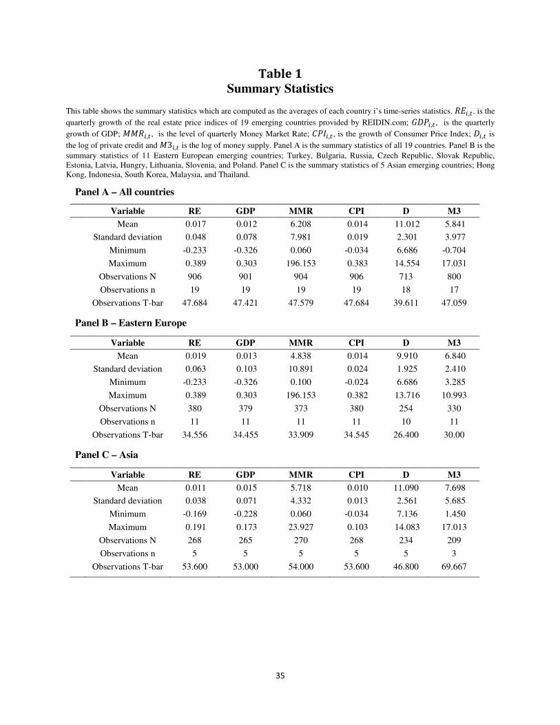
35
Table 1
Summary Statistics
This table shows the summary statistics which are computed as the averages of each country i’s time-series statistics. �!�,�. is the
quarterly growth of the real estate price indices of 19 emerging countries provided by REIDIN.com; "#$�,�, is the quarterly
growth of GDP; %%��,�, is the level of quarterly Money Market Rate; �$&�,�, is the growth of Consumer Price Index; #�,� is
the log of private credit and %3�,� is the log of money supply. Panel A is the summary statistics of all 19 countries. Panel B is the
summary statistics of 11 Eastern European emerging countries; Turkey, Bulgaria, Russia, Czech Republic, Slovak Republic, Estonia, Latvia, Hungry, Lithuania, Slovenia, and Poland. Panel C is the summary statistics of 5 Asian emerging countries; Hong Kong, Indonesia, South Korea, Malaysia, and Thailand.
Panel A – All countries
Variable RE GDP MMR CPI D M3
Mean 0.017 0.012 6.208 0.014 11.012 5.841
Standard deviation 0.048 0.078 7.981 0.019 2.301 3.977
Minimum -0.233 -0.326 0.060 -0.034 6.686 -0.704
Maximum 0.389 0.303 196.153 0.383 14.554 17.031
Observations N 906 901 904 906 713 800
Observations n 19 19 19 19 18 17
Observations T-bar 47.684 47.421 47.579 47.684 39.611 47.059
Panel B – Eastern Europe
Variable RE GDP MMR CPI D M3
Mean 0.019 0.013 4.838 0.014 9.910 6.840
Standard deviation 0.063 0.103 10.891 0.024 1.925 2.410
Minimum -0.233 -0.326 0.100 -0.024 6.686 3.285
Maximum 0.389 0.303 196.153 0.382 13.716 10.993
Observations N 380 379 373 380 254 330
Observations n 11 11 11 11 10 11
Observations T-bar 34.556 34.455 33.909 34.545 26.400 30.00
Panel C – Asia
Variable RE GDP MMR CPI D M3
Mean 0.011 0.015 5.718 0.010 11.090 7.698
Standard deviation 0.038 0.071 4.332 0.013 2.561 5.685
Minimum -0.169 -0.228 0.060 -0.034 7.136 1.450
Maximum 0.191 0.173 23.927 0.103 14.083 17.013
Observations N 268 265 270 268 234 209
Observations n 5 5 5 5 5 3
Observations T-bar 53.600 53.000 54.000 53.600 46.800 69.667

36
Figure 1
House Price Indices in Emerging Countries
This graph displays quarterly house price indices in 19 Emerging Countries
0
500
1000
1500
19
97
Q1
19
98
Q2
19
99
Q3
20
00
Q4
20
02
Q1
20
03
Q2
20
04
Q3
20
05
Q4
20
07
Q1
20
08
Q2
20
09
Q3
20
10
Q4
20
12
Q1
Bulgaria
0
50
100
150
200
250
19
93
Q1
19
94
Q2
19
95
Q3
19
96
Q4
19
98
Q1
19
99
Q2
20
00
Q3
20
01
Q4
20
03
Q1
20
04
Q2
20
05
Q3
20
06
Q4
20
08
Q1
20
09
Q2
20
10
Q3
20
11
Q4
Hong Kong
0
50
100
150
200
20
04
Q1
20
04
Q3
20
05
Q1
20
05
Q3
20
06
Q1
20
06
Q3
20
07
Q1
20
07
Q3
20
08
Q1
20
08
Q3
20
09
Q1
20
09
Q3
20
10
Q1
20
10
Q3
Czech Republic
0
500
1000
1500
20
03
Q3
20
04
Q2
20
05
Q1
20
05
Q4
20
06
Q3
20
07
Q2
20
08
Q1
20
08
Q4
20
09
Q3
20
10
Q2
20
11
Q1
20
11
Q4
Estonia
0
50
100
1502
00
1Q
4
20
02
Q3
20
03
Q2
20
04
Q1
20
04
Q4
20
05
Q3
20
06
Q2
20
07
Q1
20
07
Q4
20
08
Q3
20
09
Q2
20
10
Q1
20
10
Q4
20
11
Q3
20
12
Q2
Hungary
0
50
100
150
200
20
02
Q1
20
02
Q4
20
03
Q3
20
04
Q2
20
05
Q1
20
05
Q4
20
06
Q3
20
07
Q2
20
08
Q1
20
08
Q4
20
09
Q3
20
10
Q2
20
11
Q1
20
11
Q4
Indonesia
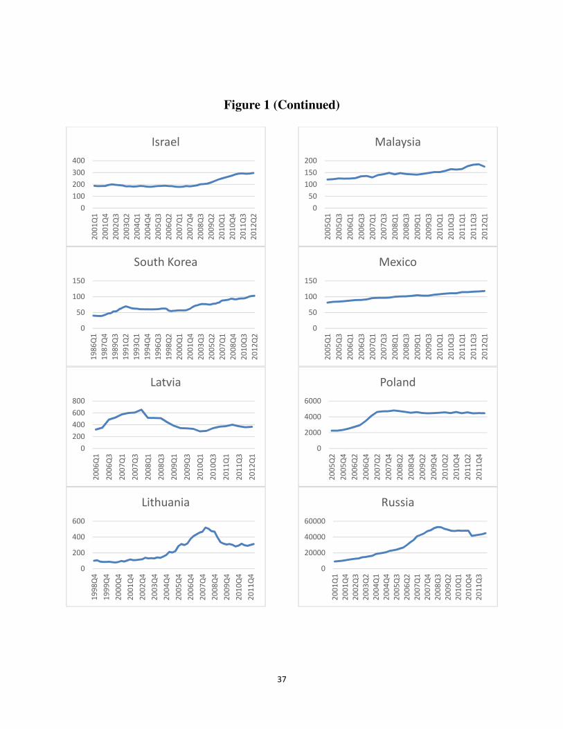
37
Figure 1 (Continued)
0
100
200
300
400
20
01
Q1
20
01
Q4
20
02
Q3
20
03
Q2
20
04
Q1
20
04
Q4
20
05
Q3
20
06
Q2
20
07
Q1
20
07
Q4
20
08
Q3
20
09
Q2
20
10
Q1
20
10
Q4
20
11
Q3
20
12
Q2
Israel
0
50
100
150
19
86
Q1
19
87
Q4
19
89
Q3
19
91
Q2
19
93
Q1
19
94
Q4
19
96
Q3
19
98
Q2
20
00
Q1
20
01
Q4
20
03
Q3
20
05
Q2
20
07
Q1
20
08
Q4
20
10
Q3
20
12
Q2
South Korea
0
200
400
600
800
20
06
Q1
20
06
Q3
20
07
Q1
20
07
Q3
20
08
Q1
20
08
Q3
20
09
Q1
20
09
Q3
20
10
Q1
20
10
Q3
20
11
Q1
20
11
Q3
20
12
Q1
Latvia
0
200
400
600
19
98
Q4
19
99
Q4
20
00
Q4
20
01
Q4
20
02
Q4
20
03
Q4
20
04
Q4
20
05
Q4
20
06
Q4
20
07
Q4
20
08
Q4
20
09
Q4
20
10
Q4
20
11
Q4
Lithuania
0
50
100
150
200
20
05
Q1
20
05
Q3
20
06
Q1
20
06
Q3
20
07
Q1
20
07
Q3
20
08
Q1
20
08
Q3
20
09
Q1
20
09
Q3
20
10
Q1
20
10
Q3
20
11
Q1
20
11
Q3
20
12
Q1
Malaysia
0
50
100
150
20
05
Q1
20
05
Q3
20
06
Q1
20
06
Q3
20
07
Q1
20
07
Q3
20
08
Q1
20
08
Q3
20
09
Q1
20
09
Q3
20
10
Q1
20
10
Q3
20
11
Q1
20
11
Q3
20
12
Q1
Mexico
0
2000
4000
6000
20
05
Q2
20
05
Q4
20
06
Q2
20
06
Q4
20
07
Q2
20
07
Q4
20
08
Q2
20
08
Q4
20
09
Q2
20
09
Q4
20
10
Q2
20
10
Q4
20
11
Q2
20
11
Q4
Poland
0
20000
40000
60000
20
01
Q1
20
01
Q4
20
02
Q3
20
03
Q2
20
04
Q1
20
04
Q4
20
05
Q3
20
06
Q2
20
07
Q1
20
07
Q4
20
08
Q3
20
09
Q2
20
10
Q1
20
10
Q4
20
11
Q3
Russia
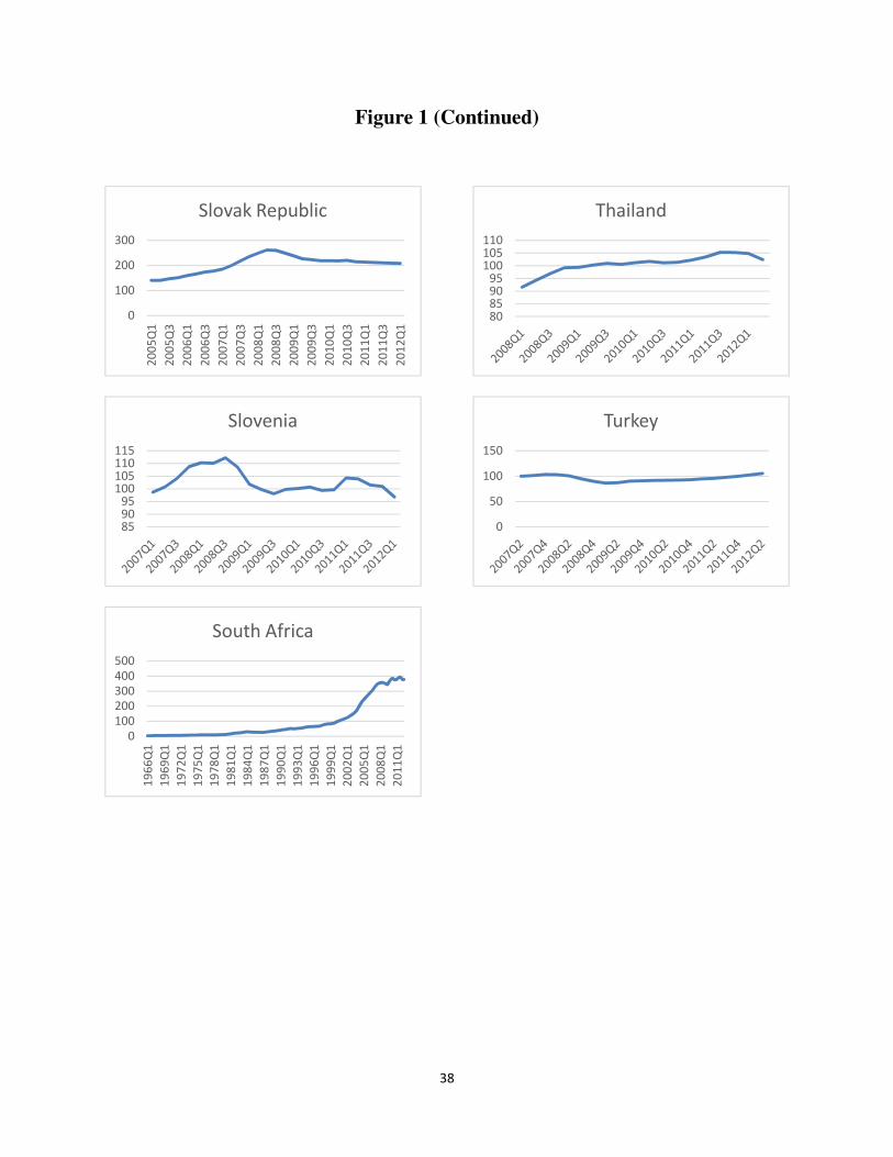
38
Figure 1 (Continued)
0
100
200
300
20
05
Q1
20
05
Q3
20
06
Q1
20
06
Q3
20
07
Q1
20
07
Q3
20
08
Q1
20
08
Q3
20
09
Q1
20
09
Q3
20
10
Q1
20
10
Q3
20
11
Q1
20
11
Q3
20
12
Q1
Slovak Republic
859095
100105110115
Slovenia
0
100
200
300
400
500
19
66
Q1
19
69
Q1
19
72
Q1
19
75
Q1
19
78
Q1
19
81
Q1
19
84
Q1
19
87
Q1
19
90
Q1
19
93
Q1
19
96
Q1
19
99
Q1
20
02
Q1
20
05
Q1
20
08
Q1
20
11
Q1
South Africa
80859095
100105110
Thailand
0
50
100
150
Turkey

39
Other variables are obtained from IFS and OECD. Missing variables are found from each
country’s central bank or other official resources. The variables that we used are; the growth of
real estate price indices, the growth of real GDP, the growth of consumer price index, the level of
the short-term nominal interest rate, the log of nominal broad money and the log of nominal
private credit.
Table 1 shows the summary statistics of the country level data which are computed as the
averages of each country’s time-series statistics. Mean, standard deviation, minimum and
maximum values and observation details are reported for the data set. Panel A is the summary
statistics of all 19 countries. Panel B is the summary statistics of 11 Eastern European emerging
countries; Turkey, Bulgaria, Russia, Czech Republic, Slovak Republic, Estonia, Latvia, Hungry,
Lithuania, Slovenia, and Poland. Panel C is the summary statistics of 5 Asian emerging
countries; Hong Kong, Indonesia, South Korea, Malaysia, and Thailand. Table 1 shows that the
mean growth of the 19 emerging markets real estate price indices is 0.017, while the growth rate
is lower in Asian emerging countries, it is actually higher in Eastern European emerging
countries.
Figure 1 shows the quarterly real estate price indices of 19 emerging markets. It is expect
to see a positive trend in house prices due to growing populations. Land is an important factor in
housing obviously and is in fixed supply, therefore housing becomes relatively scarce, and the
relative price rises. While some countries show a continuous growth in their study periods, others
show busts and booms.
Figure 2 shows the quarterly percent change in house price indices (solid line) and the
quarterly percent change in real GDP (dotted line) in 19 emerging markets. Figure 3 shows the

40
quarterly percent change in house price indices (solid line) and the quarterly percent change in
CPI (dotted line) in our sample countries.
The figures reveal that, while there might be a correlation between growth in real estate
indices and GDP as well as CPI, the relationship is not perfect at all. Growth in real estate prices
in some countries move in the same direction with growth in GDP, However, several countries
also show a deviation in the direction of this relationship. The similar pattern is also found in the
relationship between the growth in real estate price indices and the growth in CPI in these
countries. This also means that there will not be a major multicollinearity problem including
these variables in our empirical model.
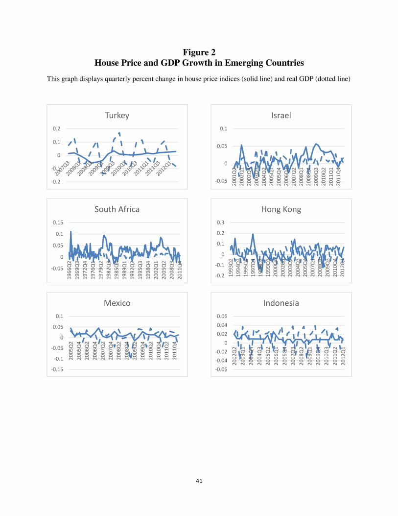
41
Figure 2
House Price and GDP Growth in Emerging Countries
This graph displays quarterly percent change in house price indices (solid line) and real GDP (dotted line)
-0.2
-0.1
0
0.1
0.2
Turkey
-0.05
0
0.05
0.1
0.15
19
66
Q2
19
69
Q3
19
72
Q4
19
76
Q1
19
79
Q2
19
82
Q3
19
85
Q4
19
89
Q1
19
92
Q2
19
95
Q3
19
98
Q4
20
02
Q1
20
05
Q2
20
08
Q3
20
11
Q4
South Africa
-0.15
-0.1
-0.05
0
0.05
0.1
20
05
Q2
20
05
Q4
20
06
Q2
20
06
Q4
20
07
Q2
20
07
Q4
20
08
Q2
20
08
Q4
20
09
Q2
20
09
Q4
20
10
Q2
20
10
Q4
20
11
Q2
20
11
Q4
Mexico
-0.05
0
0.05
0.1
20
01
Q2
20
02
Q1
20
02
Q4
20
03
Q3
20
04
Q2
20
05
Q1
20
05
Q4
20
06
Q3
20
07
Q2
20
08
Q1
20
08
Q4
20
09
Q3
20
10
Q2
20
11
Q1
20
11
Q4
Israel
-0.2
-0.1
0
0.1
0.2
0.3
19
93
Q2
19
94
Q3
19
95
Q4
19
97
Q1
19
98
Q2
19
99
Q3
20
00
Q4
20
02
Q1
20
03
Q2
20
04
Q3
20
05
Q4
20
07
Q1
20
08
Q2
20
09
Q3
20
10
Q4
20
12
Q1
Hong Kong
-0.06
-0.04
-0.02
0
0.02
0.04
0.06
20
02
Q2
20
03
Q1
20
03
Q4
20
04
Q3
20
05
Q2
20
06
Q1
20
06
Q4
20
07
Q3
20
08
Q2
20
09
Q1
20
09
Q4
20
10
Q3
20
11
Q2
20
12
Q1
Indonesia
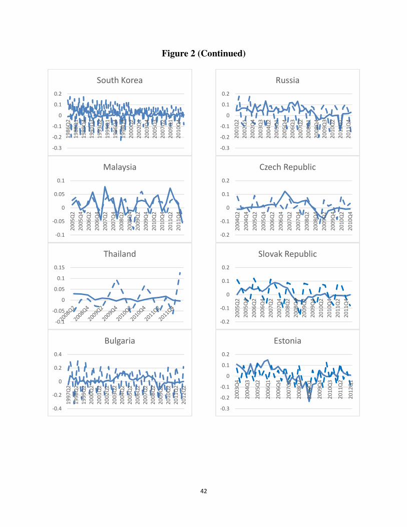
42
Figure 2 (Continued)
-0.3
-0.2
-0.1
0
0.1
0.2
19
86
Q2
19
88
Q1
19
89
Q4
19
91
Q3
19
93
Q2
19
95
Q1
19
96
Q4
19
98
Q3
20
00
Q2
20
02
Q1
20
03
Q4
20
05
Q3
20
07
Q2
20
09
Q1
20
10
Q4
South Korea
-0.1
-0.05
0
0.05
0.1
20
05
Q2
20
05
Q4
20
06
Q2
20
06
Q4
20
07
Q2
20
07
Q4
20
08
Q2
20
08
Q4
20
09
Q2
20
09
Q4
20
10
Q2
20
10
Q4
20
11
Q2
20
11
Q4
Malaysia
-0.1
-0.05
0
0.05
0.1
0.15
Thailand
-0.4
-0.2
0
0.2
0.4
19
97
Q2
19
98
Q2
19
99
Q2
20
00
Q2
20
01
Q2
20
02
Q2
20
03
Q2
20
04
Q2
20
05
Q2
20
06
Q2
20
07
Q2
20
08
Q2
20
09
Q2
20
10
Q2
20
11
Q2
20
12
Q2
Bulgaria
-0.3
-0.2
-0.1
0
0.1
0.2
20
01
Q2
20
02
Q1
20
02
Q4
20
03
Q3
20
04
Q2
20
05
Q1
20
05
Q4
20
06
Q3
20
07
Q2
20
08
Q1
20
08
Q4
20
09
Q3
20
10
Q2
20
11
Q1
20
11
Q4
Russia
-0.2
-0.1
0
0.1
0.2
20
04
Q2
20
04
Q4
20
05
Q2
20
05
Q4
20
06
Q2
20
06
Q4
20
07
Q2
20
07
Q4
20
08
Q2
20
08
Q4
20
09
Q2
20
09
Q4
20
10
Q2
20
10
Q4
Czech Republic
-0.2
-0.1
0
0.1
0.2
20
05
Q2
20
05
Q4
20
06
Q2
20
06
Q4
20
07
Q2
20
07
Q4
20
08
Q2
20
08
Q4
20
09
Q2
20
09
Q4
20
10
Q2
20
10
Q4
20
11
Q2
20
11
Q4
Slovak Republic
-0.3
-0.2
-0.1
0
0.1
0.2
20
03
Q4
20
04
Q3
20
05
Q2
20
06
Q1
20
06
Q4
20
07
Q3
20
08
Q2
20
09
Q1
20
09
Q4
20
10
Q3
20
11
Q2
20
12
Q1
Estonia
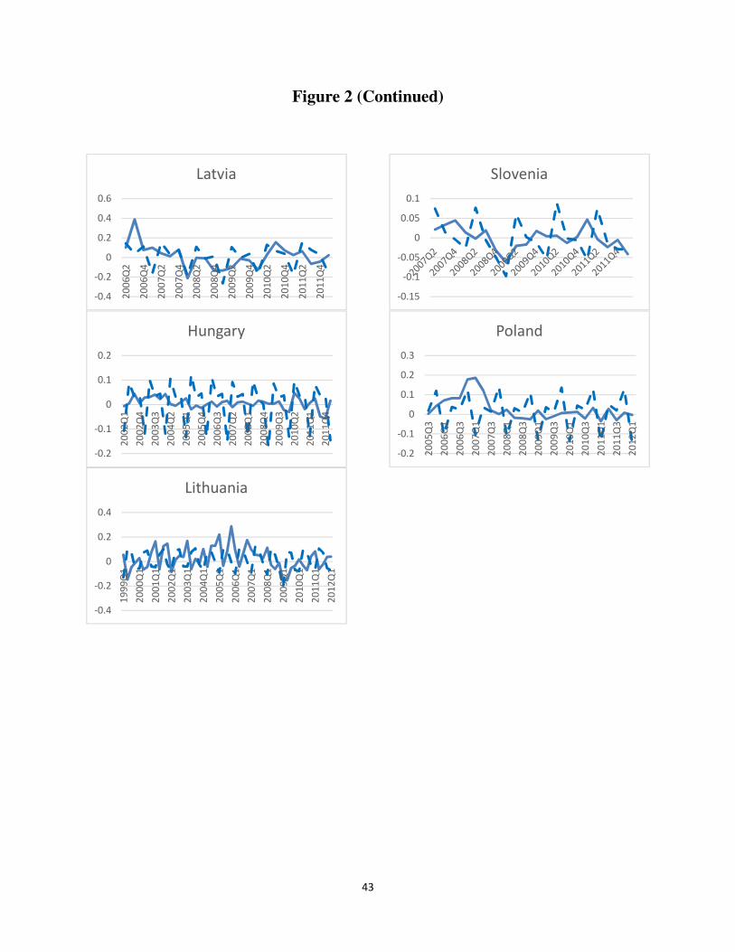
43
Figure 2 (Continued)
-0.4
-0.2
0
0.2
0.4
0.6
20
06
Q2
20
06
Q4
20
07
Q2
20
07
Q4
20
08
Q2
20
08
Q4
20
09
Q2
20
09
Q4
20
10
Q2
20
10
Q4
20
11
Q2
20
11
Q4
Latvia
-0.2
-0.1
0
0.1
0.2
20
02
Q1
20
02
Q4
20
03
Q3
20
04
Q2
20
05
Q1
20
05
Q4
20
06
Q3
20
07
Q2
20
08
Q1
20
08
Q4
20
09
Q3
20
10
Q2
20
11
Q1
20
11
Q4
Hungary
-0.4
-0.2
0
0.2
0.4
19
99
Q1
20
00
Q1
20
01
Q1
20
02
Q1
20
03
Q1
20
04
Q1
20
05
Q1
20
06
Q1
20
07
Q1
20
08
Q1
20
09
Q1
20
10
Q1
20
11
Q1
20
12
Q1
Lithuania
-0.15
-0.1
-0.05
0
0.05
0.1
Slovenia
-0.2
-0.1
0
0.1
0.2
0.3
20
05
Q3
20
06
Q1
20
06
Q3
20
07
Q1
20
07
Q3
20
08
Q1
20
08
Q3
20
09
Q1
20
09
Q3
20
10
Q1
20
10
Q3
20
11
Q1
20
11
Q3
20
12
Q1
Poland
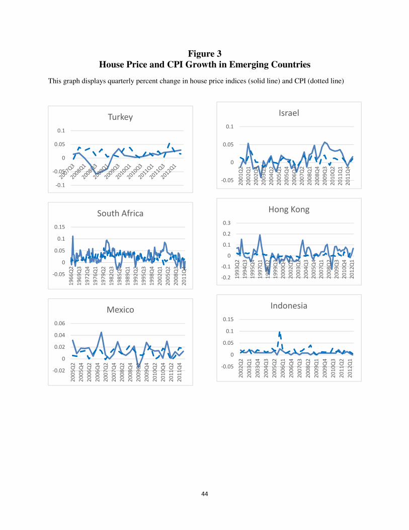
44
Figure 3
House Price and CPI Growth in Emerging Countries
This graph displays quarterly percent change in house price indices (solid line) and CPI (dotted line)
-0.1
-0.05
0
0.05
0.1
Turkey
-0.05
0
0.05
0.1
0.15
19
66
Q2
19
69
Q3
19
72
Q4
19
76
Q1
19
79
Q2
19
82
Q3
19
85
Q4
19
89
Q1
19
92
Q2
19
95
Q3
19
98
Q4
20
02
Q1
20
05
Q2
20
08
Q3
20
11
Q4
South Africa
-0.02
0
0.02
0.04
0.06
20
05
Q2
20
05
Q4
20
06
Q2
20
06
Q4
20
07
Q2
20
07
Q4
20
08
Q2
20
08
Q4
20
09
Q2
20
09
Q4
20
10
Q2
20
10
Q4
20
11
Q2
20
11
Q4
Mexico
-0.05
0
0.05
0.1
20
01
Q2
20
02
Q1
20
02
Q4
20
03
Q3
20
04
Q2
20
05
Q1
20
05
Q4
20
06
Q3
20
07
Q2
20
08
Q1
20
08
Q4
20
09
Q3
20
10
Q2
20
11
Q1
20
11
Q4
Israel
-0.2
-0.1
0
0.1
0.2
0.3
19
93
Q2
19
94
Q3
19
95
Q4
19
97
Q1
19
98
Q2
19
99
Q3
20
00
Q4
20
02
Q1
20
03
Q2
20
04
Q3
20
05
Q4
20
07
Q1
20
08
Q2
20
09
Q3
20
10
Q4
20
12
Q1
Hong Kong
-0.05
0
0.05
0.1
0.15
20
02
Q2
20
03
Q1
20
03
Q4
20
04
Q3
20
05
Q2
20
06
Q1
20
06
Q4
20
07
Q3
20
08
Q2
20
09
Q1
20
09
Q4
20
10
Q3
20
11
Q2
20
12
Q1
Indonesia
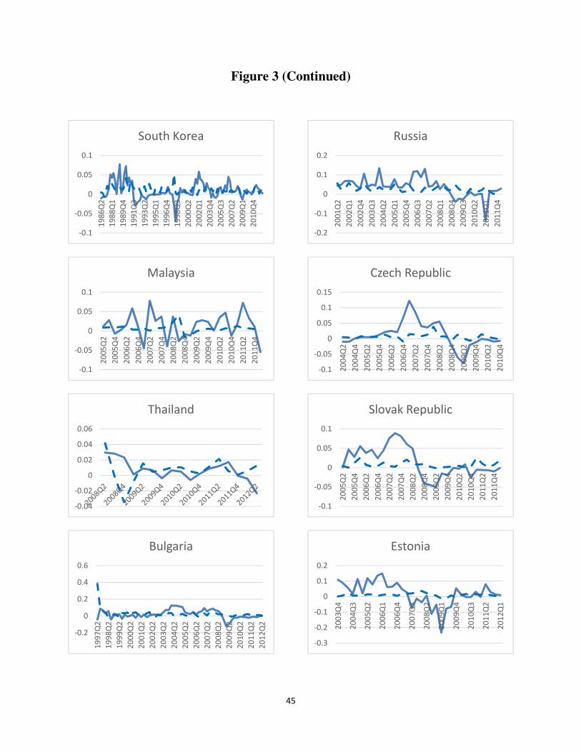
45
Figure 3 (Continued)
-0.1
-0.05
0
0.05
0.1
19
86
Q2
19
88
Q1
19
89
Q4
19
91
Q3
19
93
Q2
19
95
Q1
19
96
Q4
19
98
Q3
20
00
Q2
20
02
Q1
20
03
Q4
20
05
Q3
20
07
Q2
20
09
Q1
20
10
Q4
South Korea
-0.1
-0.05
0
0.05
0.1
20
05
Q2
20
05
Q4
20
06
Q2
20
06
Q4
20
07
Q2
20
07
Q4
20
08
Q2
20
08
Q4
20
09
Q2
20
09
Q4
20
10
Q2
20
10
Q4
20
11
Q2
20
11
Q4
Malaysia
-0.04
-0.02
0
0.02
0.04
0.06
Thailand
-0.2
0
0.2
0.4
0.6
19
97
Q2
19
98
Q2
19
99
Q2
20
00
Q2
20
01
Q2
20
02
Q2
20
03
Q2
20
04
Q2
20
05
Q2
20
06
Q2
20
07
Q2
20
08
Q2
20
09
Q2
20
10
Q2
20
11
Q2
20
12
Q2
Bulgaria
-0.2
-0.1
0
0.1
0.2
20
01
Q2
20
02
Q1
20
02
Q4
20
03
Q3
20
04
Q2
20
05
Q1
20
05
Q4
20
06
Q3
20
07
Q2
20
08
Q1
20
08
Q4
20
09
Q3
20
10
Q2
20
11
Q1
20
11
Q4
Russia
-0.1
-0.05
0
0.05
0.1
0.15
20
04
Q2
20
04
Q4
20
05
Q2
20
05
Q4
20
06
Q2
20
06
Q4
20
07
Q2
20
07
Q4
20
08
Q2
20
08
Q4
20
09
Q2
20
09
Q4
20
10
Q2
20
10
Q4
Czech Republic
-0.1
-0.05
0
0.05
0.1
20
05
Q2
20
05
Q4
20
06
Q2
20
06
Q4
20
07
Q2
20
07
Q4
20
08
Q2
20
08
Q4
20
09
Q2
20
09
Q4
20
10
Q2
20
10
Q4
20
11
Q2
20
11
Q4
Slovak Republic
-0.3
-0.2
-0.1
0
0.1
0.2
20
03
Q4
20
04
Q3
20
05
Q2
20
06
Q1
20
06
Q4
20
07
Q3
20
08
Q2
20
09
Q1
20
09
Q4
20
10
Q3
20
11
Q2
20
12
Q1
Estonia
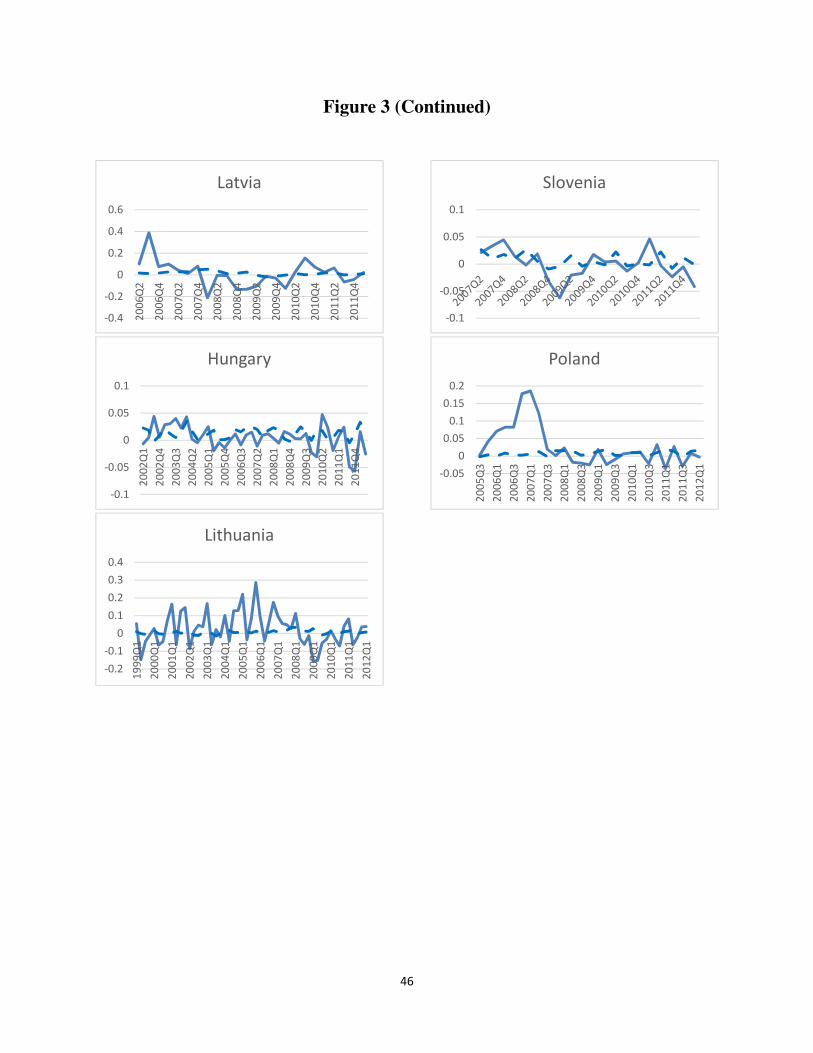
46
Figure 3 (Continued)
-0.4
-0.2
0
0.2
0.4
0.6
20
06
Q2
20
06
Q4
20
07
Q2
20
07
Q4
20
08
Q2
20
08
Q4
20
09
Q2
20
09
Q4
20
10
Q2
20
10
Q4
20
11
Q2
20
11
Q4
Latvia
-0.1
-0.05
0
0.05
0.1
20
02
Q1
20
02
Q4
20
03
Q3
20
04
Q2
20
05
Q1
20
05
Q4
20
06
Q3
20
07
Q2
20
08
Q1
20
08
Q4
20
09
Q3
20
10
Q2
20
11
Q1
20
11
Q4
Hungary
-0.2
-0.1
0
0.1
0.2
0.3
0.4
19
99
Q1
20
00
Q1
20
01
Q1
20
02
Q1
20
03
Q1
20
04
Q1
20
05
Q1
20
06
Q1
20
07
Q1
20
08
Q1
20
09
Q1
20
10
Q1
20
11
Q1
20
12
Q1
Lithuania
-0.1
-0.05
0
0.05
0.1
Slovenia
-0.05
0
0.05
0.1
0.15
0.2
20
05
Q3
20
06
Q1
20
06
Q3
20
07
Q1
20
07
Q3
20
08
Q1
20
08
Q3
20
09
Q1
20
09
Q3
20
10
Q1
20
10
Q3
20
11
Q1
20
11
Q3
20
12
Q1
Poland

47
IV. Framework
A. Predictability of Real Estate Price Index Returns
A.1. Parameter Estimates
The fixed-effects panel data regression shows the relationship between the Real Estate
Price Index returns and the independent variables; GDP, money market rate (MMR), consumer
price index (CPI), private credit (D) and money supply (M3)
rj,t = αj + βZj,t + εj,t (1)
r is index return for country j at time t and independent variables for country j are defined by Z at
time t.
Table 2
Fixed Effects Regression This table shows the parameter estimates and standard errors for real estate price index returns from the fixed effects regression results with clustered standard errors. In the regression, dependent variable is the quarterly growth on the real estate price indices
of 19 emerging countries provided by REIDIN.com; �!�,�. Independent variables are growth of "#$�,�, level of Money Market
Rate %%��,�, growth of Consumer Price Index �$&�,�, log of private credit #�,� and log of money supply%3�,�. Standard errors
are reported in parenthesis. *, **, *** indicate significance at the 10%, 5% and 1% level, respectively.
Fixed Effects Panel Regressions
Constant GDP MMR CPI D M3 ()
0.294*** 0.035 -0.002*** 0.270*** -0.055*** 0.059*** 0.16
(0.079) (0.053) (0.001) (0.100) (0.016) (0.016)

48
Table 2 shows the parameter estimates and standard errors for real estate price index
regression results. Results show that all of the coefficients, except for GDP, are statistically
significant at 1% level. Money market rate, growth in CPI, private credit and M3 are all
positively correlated with the growth in real estate price index returns. Coefficient signs also
seem to be in line with the current literature on real estate in developed countries. Quan and
Titman (1999) and Hoesli et al. (2008) found positive relationship between real estate returns
and anticipated inflation in the US and the UK. McCue and King (1994) claim that nominal short
term interest rate explains majority of the variation in real estate series.
A.2. Forecasting Real Estate Price Index Returns
To test whether house prices, credit, money and economic activity can predict one-
quarter-ahead market returns in emerging countries, fixed-effects panel data regression is used.
rj,t +1 = αj + δXj,t + ξj,t+1 (2)
r is index return for country j at time t+1 and independent variables for country j are defined by
X at time t. The lagged dependent variable is also added as a control variable. As stated by
Ferson et al. (2003) persistent dependent variables may result in a spurious regression. In panel
data, the variance-covariance matrix of the error terms is simply the combination of variance-
covariance matrices of each country which, aside from the autocorrelation of the error terms
within each country, causes a contemporaneous cross-sectional correlation. This can inflate the t-
statistics by a significant amount. To correct this, we compute standard errors in the existence of
heteroskedasticity and contemporaneous cross-correlations as suggested by Rogers (1983, 1993).
By estimating intercepts, α, separately for each country j, we lower to the country-level data and
make sure that each country’s error term is orthogonal to the explanatory variables for that

49
country. Therefore, in a panel data form using fixed effects regression, the results reject the time-
series relation between the dependent and independent variables. In equation (2), the slope
coefficient, δ, together with its clustered standard errors, shows whether there is a statistically
significant relation between thee real estate price index returns and broad money, private credit
and macro economy.
Table 3
Forecasting Real Estate Price Index This table shows the parameter estimates and standard errors for real estate price index returns from the fixed effects regression results with clustered standard errors. In the regression, dependent variable is the lead quarterly growth of the real estate price
indices of 19 emerging countries provided by REIDIN.com; �!�,�*�. Independent lagged variables are growth of the real estate
price index; �!�,�, growth of "#$�,�, level of Money Market Rate %%��,�, growth of Consumer Price Index �$&�,�, log of
private credit #�,� and log of money supply %3�,�. Clustered standard errors are reported in parenthesis. *, **, *** indicate
significance level at the 10%, 5% and 1%, respectively.
Fixed Effects Panel Regressions
Constant RE GDP MMR CPI D M3 ()
1 0.016*** 0.053 0.04
(0.003) (0.038)
2 0.021*** -0.001** 0.05
(0.003) (0.001)
3 0.015*** 0.176*** 0.04
(0.003) (0.066)
4 0.042* -0.002 0.06
(0.024) (0.002)
5 0.029*** -0.002* 0.06
(0.006) (0.001)
6 0.193*** 0.491*** 0.061** -0.001** 0.216* -0.037*** 0.040*** 0.37
(0.058) (0.062) (0.024) (0.001) (0.130) (0.011) (0.022)

50
Table 3 shows the univariate regression of the one quarter ahead real estate price index
returns on growth of GDP, level of MMR, growth of CPI, log of D and log of M3. Second row
shows that the money market rate is negatively correlated with the future growth in real estate
price index returns at 5% significance level with a t-statistics of -2.56 when it is regressed alone.
Growth in money supply, M3, as seen in row five, is also negatively correlated with the future
growth in real estate price index returns at 10% level with a t-statistics of -1.74 when it is
regressed alone. Both variables have statistically significant predictive power. On the other hand,
third row reveals that growth in CPI is positively correlated with the future growth in real estate
price index returns at 1% level with a t-statistics of 2.67. CPI has a strong predictive power.
When we regress all of the variables together, we see that all of our variables significantly
predicts the growth in real estate price index returns. Interestingly in this setting, GDP and
private credit have forecasting power so they are statistically significant as opposed to when they
were regressed by themselves. The coefficient of GDP is 0.061 with a t-statistics of 2.54,
whereas the coefficient of D is -0.037 with a t-statistics of -3.32. This means that when there is a
positive growth in private credit, the real estate price indices tend to be negatively affected from
this the following quarter. We explain this by the lack of organized mortgage markets in
emerging markets as well as the structure of financial institutions. When private credit to
businesses increase, available money to the real estate markets might be declining therefore
affecting the growth in prices negatively. Our results show that there is a strong negative
correlation between the growth in real estate price indices and the lagged money market rates
and private credit. There is a strong positive correlation between the growth in real estate price
indices and the lagged growth in GDP, CPI and log of M3.

51
We wanted to see if the predictive power of these variables is different for different
regions. When we regress one quarter ahead real estate price index returns on our money, credit
and macro variables in Eastern European emerging markets and Asian emerging markets in our
sample, we actually get different results. Table 4 reveals that in Eastern Europe, only GDP has
predictive power a quarter ahead at 5% significance level. The other variables are not statistically
significant even at 10% level. However in Asian emerging countries, money market rate, private
credit and money supply have significantly predictive power at 1% level.
Table 4
Forecasting Real Estate Price Index for Different Regions This table shows the parameter estimates and standard errors for real estate price index returns from the fixed effects regression results with clustered standard errors. In the regression, dependent variable is the lead quarterly growth of the real estate price
indices provided by REIDIN.com; �!�,�*�. Independent lagged variables are growth of the real estate price index; �!�,�, growth
of "#$�,�, level of Money Market Rate %%��,�, growth of Consumer Price Index �$&�,�, log of private credit #�,� and log of
money supply %3�,�. Panel A is the fixed effects regression results of 11 Eastern European emerging countries; Turkey,
Bulgaria, Russia, Czech Republic, Slovak Republic, Estonia, Latvia, Hungry, Lithuania, Slovenia, and Poland. Panel B is the fixed effects regression results of 5 Asian emerging countries; Hong Kong, Indonesia, South Korea, Malaysia, and Thailand. Clustered standard errors are reported in parenthesis. *, **, *** indicate significance level at the 10%, 5% and 1%, respectively.
Panel A - Fixed Effects Panel Regression for Eastern Europe
Constant RE GDP MMR CPI D M3 ()
0.140* 0.458*** 0.083** -0.001 0.261 -0.037 0.037 0.32
(0.075) (0.079) (0.039) (0.002) (0.266) (0.034) (0.045)
Panel B - Fixed Effects Panel Regression for Asia
Constant RE GDP MMR CPI D M3 ()
0.305*** 0.484*** 0.006 -0.003*** 0.094 -0.060*** 0.050*** 0.48
(0.063) (0.084) (0.024) (0.001) (0.182) (0.016) (0.016)
52
B. Relationship among house prices, credit, money and economic activity
The analysis is quarterly data for 19 emerging markets spanning the period 1966-2012.
To investigate the relationship among our variables as well as the direction of the relationship,
we used Vector Auto-regression, Granger Causality, and Variance Decomposition analysis. The
estimation of a Vector Auto-regression, VAR model, introduces by Sims (1980), requires two
steps. First, a vector of variables dated at time t is regressed on several lags of itself. The
residuals from these regressions are interpreted as innovations which show the new information
about the variables that became available during period t. In the second step of estimation, these
innovations are regressed on themselves, using one of several statistical procedures. The second-
stage regressions are often given a structural or behavioral interpretation. Therefore, the residuals
from the second-stage regressions are often viewed as structural shocks.
Yt = AYt-1 + … + A’Yt-k + et (3)
where k is the number of lags that is considered in the system Yt, Yt-1,…,Yt-k equals to the 1 x p
vector of variables and A,…,A' equal to the p x p matrices of coefficients to be estimated. Also et
is an 1 x p vector of innovations that may be contemporaneously correlated but are uncorrelated
with their own lagged values and uncorrelated with all of the right-hand side variables.
B.1. Unit Root Test
For the co-integration methodology, at least two of the series should be non-stationary
process that contains a single unit root. If Yt ~ I(1), then Zt = Yt – Yt-1 is stationary. We used
Augmented Dickey-Fuller test on all of the variables for each country separately. We took first
differences of all the variables that are non-stationary to make them stationary. We also used
Akaike and Schwarz criterions to determine the lag lengths for each country. Estimating the six

53
dimensional VAR at the individual country level can suffer from too few degrees of freedom
especially if there is missing data which is very common for macro variables. We had to drop
some of the variables in some countries to get around this problem, especially the variables that
have significant missing quarterly data.
B.2. Granger Causality Test
In a regression analysis, we look at the dependence of one variable on other variables, but
it does not necessarily show the causation. In other words, the existence of a relationship
between variables does not prove causality or the direction of the influence.
Granger (1969) developed a test approach to prove that a time series X contribute to the
prediction of another series, Y. In this section the relationship among real estate price index
returns, GDP, inflation, money market rate, private credit and money supply are investigated
using Granger Causality tests.
Table 5 displays the results from the Granger causality tests for each country, which
reveals strong evidence of multi-directional causality between house prices, GDP, CPI, interest
rates, money, and credit. In Hong Kong, Lithuania, Mexico and Poland, for example, the
relationship between house prices and GDP is in both directions; GDP has a significant effect on
the future house prices and house prices also have significant effect on the future GDP. This
multi-directional relationship also exists between CPI and house prices in Hong Kong and
Lithuania. There is also a multidirectional link between MMR and house prices in Czech
Republic, South Africa and South Korea. Finally in Czech Republic the direction of relationship
between private credit and house prices is both ways.

54
Table 5
Granger Causality Test This table shows the direction of granger causality tests conducted in each country. ∆REI is the growth of the real estate price index; ∆GDP is the growth of GDP; MMR is the level of Money Market Rate; ∆CPI is the growth of Consumer Price Index, ∆D is the log of private credit, and ∆M3 is the log of money supply. P values are in parenthesis.
∆GDP → ∆REI ∆REI → ∆GDP ∆GDP ↔ ∆REI
Hong Kong (0.09) Bulgaria(0.01) Hong Kong
Lithuania (0.01) Estonia (0.04) Lithuania
Mexico (0.02) Hong Kong (0.01) Mexico
Poland (0.08) Lithuania (0.01) Poland
Mexico (0.07)
Poland (0.01)
Russia (0.01)
Slovak Republic (0.01)
South Africa (0.01)
Turkey (0.01)
∆CPI → ∆REI ∆REI → ∆CPI ∆CPI ↔ ∆REI
Hong Kong (0.09) Hong Kong (0.01) Hong Kong
Hungary (0.04) Indonesia (0.03) Lithuania
Latvia (0.04) Lithuania (0.01)
Lithuania (0.09) Slovak Republic (0.01)
Mexico (0.02) South Korea (0.01)
Thailand (0.05)

55
Table 5 (Continued)
MMR → ∆REI ∆REI → MMR MMR ↔ ∆REI
Czech Republic (0.09) Bulgaria (0.01) Czech Republic
Estonia (0.09) Czech Republic (0.09) South Africa
Israel (0.01) Hungary (0.04) South Korea
South Africa (0.02) South Africa (0.01)
South Korea (0.02) South Korea (0.02)
Turkey (0.04)
∆M3 → ∆REI ∆REI → ∆M3 ∆M3 ↔ ∆REI
Hong Kong (0.01) Czech Republic (0.01)
Malaysia (0.01)
∆D → ∆REI ∆REI → ∆D ∆D ↔ ∆REI
Czech Republic (0.01) Bulgaria (0.01) Czech Republic
Indonesia (0.07) Czech Republic (0.03)
Hong Kong (0.04)
Lithuania (0.02)
Russia (0.04)
It is also interesting to see that in almost every country, house prices significantly affect
the future broad money, private credit and macro variables. This has an important implication for
the policy makers in these countries as well as the potential investors to those countries. Central
banks do not necessarily implement policies to influence the future house prices, however our

56
results show that their policies can actually influence future house prices as well as the house
prices strongly influence future broad money and private credit growth levels.
B.3. Variance Decomposition
In order to decompose the variance of each element of Yt in equation 3 into components
due to each of the elements of the error term and to do so for various horizons, we conduct
variance decomposition analysis. In this analysis we are trying to see how much of the variance
of each element of Yt is due to the first error term and how much due to the second error term
and so on.
Our findings show an interesting picture for 19 emerging markets. Table 6 presents that
the forecast errors of real estate price index returns are mainly attributable to their own
innovations in Bulgaria, Czech Republic, Slovak Republic, Slovenia, and South Africa in the
following quarter. However, in Israel, only 33% is attributable to its own innovation whereas
38% of the forecast error variance is explained by the innovations in CPI. In Estonia, Indonesia,
Israel, Poland and Thailand less than 60% of the forecast errors are explained by their own
innovations. Interestingly in Poland, innovations in CPI explain more than 46% of the forecast
error variance to real estate price index returns. When we look at the second quarter horizon in
table 6, also in Hong Kong, Lithuania, Malaysia, Mexico, Russia and Turkey less than 60% of
the forecast errors are explained by their own innovations. In almost every country we
investigated, forecast errors to GDP, CPI, and money market rate play an important role in
explaining innovations to the real estate price index returns.
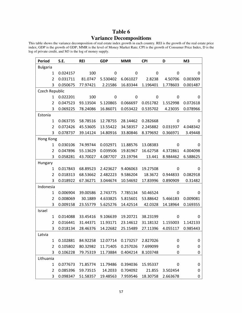
57
Table 6
Variance Decompositions This table shows the variance decomposition of real estate index growth in each country. REI is the growth of the real estate price index; GDP is the growth of GDP; MMR is the level of Money Market Rate; CPI is the growth of Consumer Price Index, D is the log of private credit, and M3 is the log of money supply.
Period S.E. REI GDP MMR CPI D M3
Bulgaria
1 0.024157 100 0 0 0 0 0
2 0.031711 81.0747 5.530402 6.061027 2.8238 4.50706 0.003009
3 0.050675 77.97421 2.21586 16.83344 1.196401 1.778603 0.001487
Czech Republic
1 0.022201 100 0 0 0 0 0
2 0.047523 93.13504 5.120865 0.066697 0.051782 1.552998 0.072618
3 0.069225 78.24086 16.86071 0.053422 0.535702 4.23035 0.078966
Estonia
1 0.063735 58.78516 12.78755 28.14462 0.282668 0 0
2 0.072426 45.53605 13.55422 34.58357 2.245882 0.031937 4.048342
3 0.078737 39.14124 14.80916 33.80846 8.379692 0.366971 3.49448
Hong Kong
1 0.030106 74.99744 0.032971 11.88576 13.08383 0 0
2 0.047896 55.13629 0.039506 19.81967 16.62758 4.372861 4.004098
3 0.058281 43.70027 4.087707 23.19794 13.441 8.984462 6.588625
Hungary
1 0.017843 68.89523 2.423627 9.406063 19.27508 0 0
2 0.018313 68.53662 2.482223 9.586204 18.3672 0.944833 0.082918
3 0.018922 67.36271 3.044674 10.54692 17.83996 0.890909 0.31482
Indonesia
1 0.006904 39.00586 2.743775 7.785134 50.46524 0 0
2 0.008069 30.1889 4.633825 5.815601 53.88642 5.466183 0.009081
3 0.009158 23.55779 5.625276 14.42514 42.0328 14.18964 0.169355
Israel
1 0.014088 33.45416 9.106639 19.20721 38.23199 0 0
2 0.016441 31.44371 11.93171 23.14612 31.18132 1.155003 1.142133
3 0.018134 28.46376 14.22682 25.15489 27.11396 4.055117 0.985443
Latvia
1 0.102881 84.92258 12.07714 0.173257 2.827026 0 0
2 0.105802 80.32982 11.71405 0.257026 7.699099 0 0
3 0.106228 79.75319 11.73884 0.404214 8.103748 0 0
Lithuania
1 0.077673 71.85774 11.79486 0.394036 15.95337 0 0
2 0.085396 59.73515 14.2033 0.704092 21.855 3.502454 0
3 0.098347 51.58357 19.48563 7.959546 18.30758 2.663678 0

58
Table 6 (Continued)
Period S.E. REI GDP MMR CPI D M3
Malaysia
1 0.035419 62.15115 24.48083 4.723128 8.644898 0 0
2 0.044953 47.3974 37.29059 3.076149 12.11371 0 0.122148
3 0.045099 47.09465 37.06453 3.121785 12.10755 0 0.61148
Mexico
1 0.009546 70.06695 0.004049 28.69054 1.238463 0 0
2 0.01064 56.39961 7.084196 24.06984 10.19012 0 2.25623
3 0.011372 51.64943 8.238863 24.71749 13.01386 0 2.380353
Poland
1 0.040745 21.6541 4.496019 27.24993 46.59995 0 0
2 0.048746 24.75313 9.648047 28.18578 37.32417 0 0.088874
3 0.060885 28.26724 8.110692 28.71206 32.15057 0 2.759436
Russia
1 0.037977 70.56521 18.56186 0.485193 10.38773 0 0
2 0.043642 53.50575 16.19698 0.778594 25.58018 0.951301 2.987207
3 0.047568 51.42839 14.07409 0.907194 21.53531 0.871043 11.18397
Slovak Republic
1 0.018012 100 0 0 0 0 0
2 0.025347 99.76028 0.061759 0 0.177958 0 0
3 0.034925 98.68466 0.204 0 1.111337 0 0
Slovenia
1 0.032443 100 0 0 0 0 0
2 0.036588 96.74549 1.225553 0 0.116883 0 1.912072
3 0.037587 94.26179 3.09955 0 0.141117 0 2.497541
South Africa
1 0.012137 99.64917 0.17224 0.101014 0.077571 0 0
2 0.017433 93.58635 0.125583 3.793401 0.13879 1.380478 0.975399
3 0.020111 86.71716 0.576669 7.915657 0.37984 2.996521 1.414152
South Korea
1 0.013546 85.33999 10.33327 0.045611 4.281133 0 0
2 0.017821 65.14771 22.9192 7.732547 3.763197 0.126361 0.310983
3 0.022263 47.89443 24.49571 17.4917 4.504618 5.40568 0.207866
Thailand
1 0.009175 14.88978 0.444163 19.9962 64.66986 0 0
2 0.011393 11.03682 32.17626 14.41466 42.37226 0 0
3 0.011833 11.06525 30.71152 13.85177 44.37147 0 0
Turkey
1 0.013866 84.12949 0.001894 6.342265 9.526354 0 0
2 0.0273 54.16049 1.609169 4.251012 39.63942 0 0.339912
3 0.034881 41.07273 1.133549 5.608226 51.90887 0 0.276629

59
V. Conclusion
Real estate is undoubtedly one of the most important components of a national economy.
This is also true for emerging countries. However, there is not enough empirical evidence
regarding their interaction with money, private credit and macro economy. The main objectives
of central banks are not necessarily in line with the goals of asset prices, particularly house
prices; however house price changes can have important implications for economic activity and
inflation. The consequences of substantial changes in house prices should also be watched
carefully by central banks and other government agencies that regulate financial institutions for
the purpose of financial stability. 2008 crises showed that the real estate prices have important
effects on the overall economy. Emerging markets have been relatively less affected by this
crises compared to the developed markets.
Using the fixed effects panel data approach, this paper analyzes the variation in 19
emerging markets real estate index returns. Our results show that money market rate, growth in
GDP and CPI as well as log of private credit (D) and money supply (M3) have significant
predictive power on growth in real estate price indices a quarter ahead. There is a strong negative
correlation between the growth in real estate price indices and the lagged money market rates
and private credit. There is a strong positive correlation between the growth in real estate price
indices and the lagged growth in GDP, CPI and log of M3. When we look at different regions,
we show that in Eastern Europe only GDP has a predictive power whereas in Asia MMR, D as
well as M3 have statistically significant predictive power.
Granger causality tests for each country reveals strong evidence of multi-directional link
between house prices, GDP, CPI, interest rates, money, and credit. House prices significantly
affect the future broad money, private credit and macro variables. When we look at the variance

60
decomposition, in almost every country we investigated, forecast errors to GDP, CPI and money
market rate play an important role in explaining innovations to the real estate price index returns.
Findings of this study may have important implications over the macro and monetary
policies of the emerging markets. There has been a dramatic increase in REIT funds in the last
decade. Emerging markets REIT funds also have become important tool in investments. Since
the underlying asset of REITs are the real estate prices, finding variables that have important
implications in a lead-lag relationship can also have important implication on these funds.
Empirical findings of this paper do not necessarily support this analysis therefore a future
research on the variables we investigated and REITs can present important implications for
investors on more liquid assets like REITs.
References
• Ahearne, A. G., Ammer, J., Doyle, B. M., Kole, L. S. and Martin, R. F., 2005, Monetary
Policy and House Prices: A Cross-Country Study, FRM International Finance Discussion
paper No. 841.
• Aizenman, J. and Yothin, J, 2009, Current account patterns and national real estate
markets, Journal of Urban Economics
• Baffoe-Bonnie, J. 1998, The Dynamic Impact of Macroeconomic Aggregates on Housing
Prices and Stock of Houses: A National and Regional Analysis, Journal of Real Estate
Finance & Economics.
• Ball, M. The 1980s Property Boom. Environment and Planning A, 1994, 26, 671-695.

61
• Beltratti, A. and C. Morana. International house prices and macroeconomic fluctuations.
Journal of Banking and Finance, 2010, 34, 533-545.
• Breedon, F. and M.A.S. Joyce. House Prices, Arrears, and Possessions. Bank of England
Quarterly Bulletin, 1992, 173-179.
• Darrat, A.F. and J.L. Glascock. Real Estate Return, Money and Fiscal Deficits: Is the
Real Estate Market Efficient? Journal of Real Estate Finance and Economics, 1989, 2,
197-208.
• Ewing, B. T., Payne, J. E., 2005, The response of real estate investment trust returns to
macroeconomic shocks, Journal of Business Research
• Gilchrist, S. and J.V. Leahy. Monetary Policy and Asset Prices, Journal of Monetary
Economics, 2002, 49:1, 75-97.
• Goodhart, C., 2007, Whatever Became of the Monetary Aggregates, National Institute
Economic Review
• Goodhart, C. and Hofmann, B., 2008 House prices, money, credit, and the
macroeconomy. Oxford Review of Economic Policy.
• Greiber, C. and R. Setzer, 2007, Money and Housing – Evidence for the Euro Area and
the US, Deutsche Bundesbank Discussion Paper, Series 1: Economic Studies
• Gyourko, J. and Keim, D. (1992), What Does the Stock Market Tell Us About Real
Estate Returns, Journal of the American Real Estate and Urban Economics Association.
• Jin, Y. and Z. Zeng. Residential Investment and House Prices in a Multi-sector Monetary
Business Cycle Model. Journal of Housing Economics, 2004, 13, 268-286

62
• Kasparova, D., and White, M. (2001), The Responsiveness Of House Prices To
Macroeconomic Forces: A Cross-Country Comparison, European Journal of Housing
Policy.
• Kim, DK., 2005, Money and Its Effect on U.S. Housing Sub-Markets: Evidence from the
VAR Model, Journal of Business & Economics Research
• Kishor, N. K., 2007, Does Consumption Respond More to Housing Wealth Than to
Financial Market Wealth? If So, Why?, Journal of Real Estate Finance & Economics.
• Lastrapes, W.D. The Real Price of Housing and Money Supply Shocks: Time Series
Evidence and Theoretical Simulations. Journal of Housing Economics, 2002, 11:1, 40-74
• Lin, T. C., Lin, Z., 2011, Are stock and real estate markets integrated? An empirical
study of six Asian economies, Pacific-Basin Finance Journal
• Liow, K. H., Webb, J. R., 2009, Common factors in international securitized realestate
markets, Review of Financial Economics
• Maroney, N. and Safa, M., 2012, Bid-Ask Spread, Futures Market Sentiment and
Exchange Rate Returns, Journal of Economic Cooperation and Development.
• McCue, T. E., and Kling, J. L., 1994, Real estate returns and the macroeconomy: some
empirical evidence from real estate investment trust data, 1972-1991, Journal of Real
Estate Research
• Mei, J. and Lee, A., 1994, Is There a Real Estate Factor Premium, The Journal of Real
Estate Finance and Economics
• Miller, N., Peng, L., Sklarz, M. 2009, House Price and Economic Growth, The Journal of
Real Estate Finance and Economics

63
• Myer, N., and Webb, J. R., 1993, Return Properties of Equity REITs, Common Stocks,
and Commercial Real Estate: A Comparison., Journal of Real Estate Research
• Nelson, E. (2003), The future of monetary aggregates in monetary policy analysis,
Journal of Monetary Economics.
• Schatz, A. 2009, Dynamics on real estate and emerging markets, Dissertation, University
of Regensburg
• Seiler, M. J., Webb, J. T., and Myer N. F. C., 1999, Diversification Issues in Real Estate
Investment, Journal of Real Estate Literature

64
Appendix A
Definition of Ratios
Measures Ratios Definition
Liquidity analysis Current ratio Current assets/current liabilities
Quick ratio Quick assets/current liabilities
Net working capital ratio Current assets-Current liabilities / Total Assets
Activity analysis Asset turnover ratio Sales/Average total assets
Accounts receivable
turnover ratio
Sales/Average accounts receivable
Inventory turnover ratio Cost of goods sold/Average inventories
Management
efficiency
Cost-to-income Operating expenses/operating income
Expense-to-assets Operating expenses/average assets
Earnings ability Gross profit margin Net profit/Revenue
Return on asset (ROA) Net profit before interest and tax/average
shareholders equity
Return on equity (ROE) Net profit after tax/average shareholders equity
Labor Growth in staff levels % change in the number of employees
Employee productivity Revenue/number of employees
Over employment proxy Total assets/number of employees

65
Appendix B
Monthly Data Starting Date Ending Date
HONG KONG SAR Jan-93 May-12
ISRAEL Jan-01 Apr-12
KOREA Jan-86 Jun-12
THAILAND Mar-08 May-12
SOUTH AFRICA Jan-66 Jun-12
TURKEY Jun-07 Jun-12
Quarterly Data Starting Date Ending Date
BULGARIA 1997Q1 2012Q2
CZECH REPUBLIC 2004Q1 2010Q4
ESTONIA 2003Q3 2012Q1
HUNGARY 2001Q4 2012Q2
INDONESIA 2002Q1 2012Q2
LITHUANIA 1998Q4 2012Q1
LATVIA 2006Q1 2012Q1
MEXICO 2005Q1 2012Q1
MALAYSIA 2005Q1 2012Q1
POLAND (5 MISSING OBSERVATIONS) 2002Q4 2012Q1
ROMANIA 2009Q1 2012Q1
RUSSIA 2001Q1 2012Q1
SLOVENIA 2007Q1 2012Q1
SLOVAK REPUBLIC 2005Q1 2012Q1

66
Vita
Bora Ozkan was born in Ankara, Turkey. He received his Bachelor of Science degree in
Economics in 2000 from Hacettepe University in Ankara, Turkey. He came to New Orleans,
Louisiana in 2001 as an intern for an international distribution company. He worked as a market
research analyst for the same company before he became the director of international marketing
for a global accounts receivables management firm until 2008. He received his Master of
Business Administration (MBA) degree with a concentration in finance in 2007 and Master of
Science in Financial Economics in 2010 from the University of New Orleans. Mr. Ozkan is
scheduled to receive his Ph.D. in Financial Economics from the University of New Orleans in
December 2013.
Recommended