MIT Center for Transportation & Logistics
CTL.SC1x -Supply Chain & Logistics Fundamentals
Single Period Inventory Model: Calculating Expected Profitability
CTL.SC1x - Supply Chain and Logistics Fundamentals Lesson: Expected Profits for Single Period Inventory Models
Agenda
• Expected Profits • Expected Units Short • Unit Normal Loss Function • NFL Jersey Example
2
CTL.SC1x - Supply Chain and Logistics Fundamentals Lesson: Expected Profits for Single Period Inventory Models
Expected Profits
3
CTL.SC1x - Supply Chain and Logistics Fundamentals Lesson: Expected Profits for Single Period Inventory Models 4
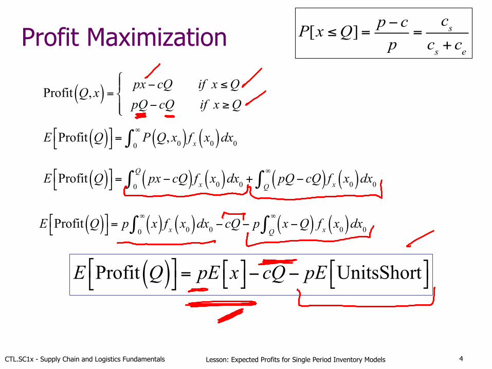
Profit Maximization P[x ≤Q]= p− cp
=cs
cs + ce
Profit Q,x( ) = px − cQ if x ≤QpQ − cQ if x ≥Q
$%&
'&
E Profit Q( )!"
#$= P Q,x0( )0
∞
∫ f x x0( )dx0
E Profit Q( )!"
#$= px − cQ( )0
Q
∫ f x x0( )dx0 + pQ − cQ( )Q
∞
∫ f x x0( )dx0
E Profit Q( )!"
#$= pE x!" #$− cQ − pE UnitsShort!" #$
E Profit Q( )!"
#$= p x( )0
∞
∫ f x x0( )dx0 − cQ − p x −Q( ) f x x0( )dx0Q
∞
∫
CTL.SC1x - Supply Chain and Logistics Fundamentals Lesson: Expected Profits for Single Period Inventory Models 5
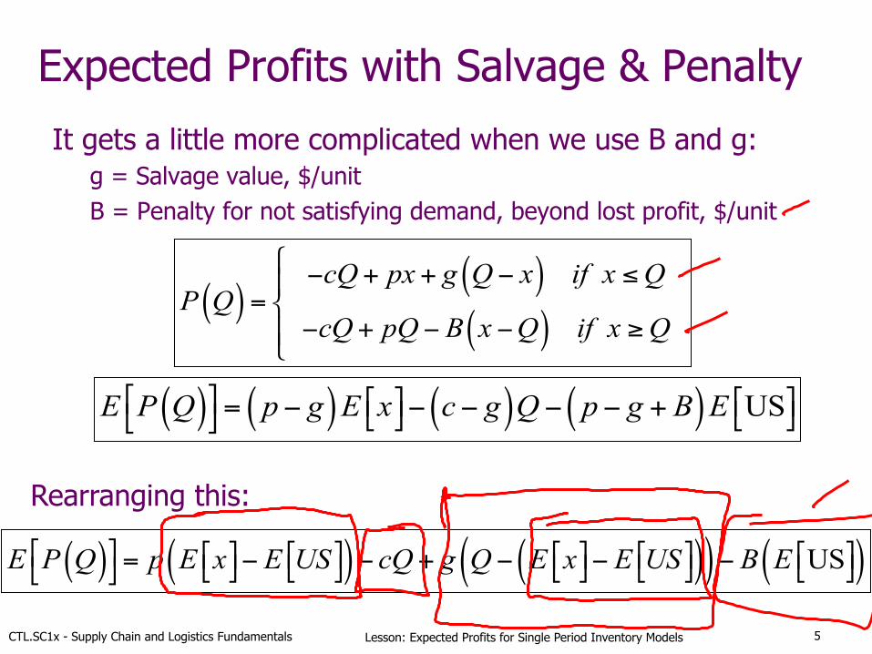
Expected Profits with Salvage & Penalty
It gets a little more complicated when we use B and g: g = Salvage value, $/unit B = Penalty for not satisfying demand, beyond lost profit, $/unit
E P Q( )!"
#$= p− g( )E x!" #$− c− g( )Q − p− g + B( )E US!" #$
P Q( ) =−cQ+ px + g Q − x( ) if x ≤Q
−cQ+ pQ − B x −Q( ) if x ≥Q
$
%&
'&
E P Q( )!"
#$= p E x!" #$− E US!" #$( )− cQ+ g Q − E x!" #$− E US!" #$( )( )− B E US!" #$( )
Rearranging this:
CTL.SC1x - Supply Chain and Logistics Fundamentals Lesson: Expected Profits for Single Period Inventory Models
Expected Units Short
6
CTL.SC1x - Supply Chain and Logistics Fundamentals Lesson: Expected Profits for Single Period Inventory Models
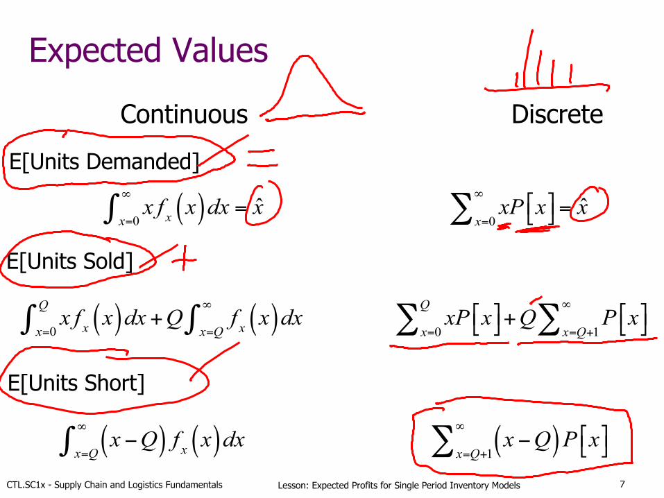
Expected Values
xx=0
∞
∫ f x x( )dx = x̂ xP x#$ %&x=0
∞
∑ = x̂
xx=0
Q
∫ f x x( )dx +Q fx x( )dxx=Q
∞
∫ xP x#$ %&x=0
Q∑ +Q P x#$ %&x=Q+1
∞
∑
x −Q( ) f x x( )dxx=Q
∞
∫ x −Q( )P x$% &'x=Q+1
∞
∑
Continuous Discrete
E[Units Demanded]
E[Units Sold]
E[Units Short]
7
CTL.SC1x - Supply Chain and Logistics Fundamentals Lesson: Expected Profits for Single Period Inventory Models
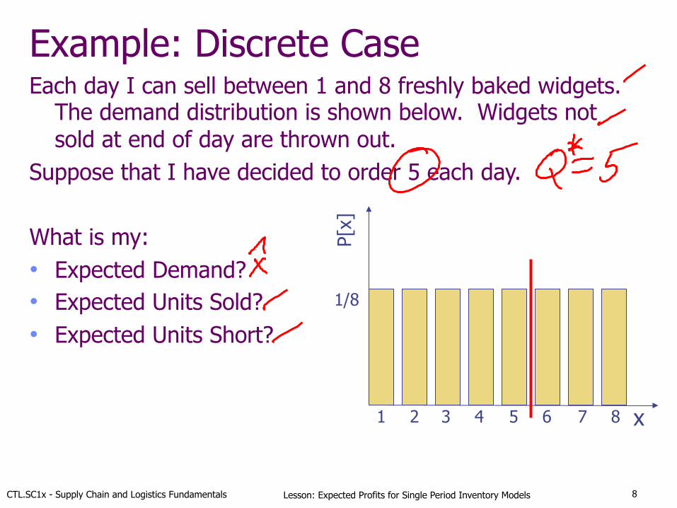
Example: Discrete Case Each day I can sell between 1 and 8 freshly baked widgets.
The demand distribution is shown below. Widgets not sold at end of day are thrown out.
Suppose that I have decided to order 5 each day. What is my: • Expected Demand? • Expected Units Sold? • Expected Units Short?
x
P[x]
1 2 3 4 5 6 7 8
1/8
8
CTL.SC1x - Supply Chain and Logistics Fundamentals Lesson: Expected Profits for Single Period Inventory Models
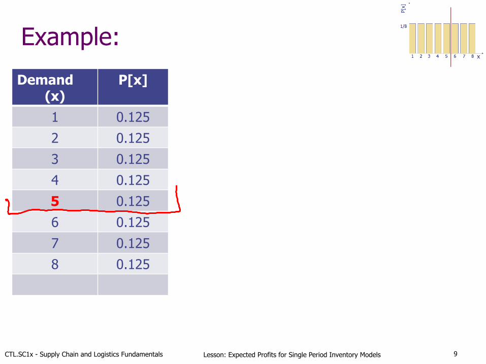
Example:
Demand (x)
P[x]
1 0.125
2 0.125
3 0.125
4 0.125
5 0.125
6 0.125
7 0.125
8 0.125
9
CTL.SC1x - Supply Chain and Logistics Fundamentals Lesson: Expected Profits for Single Period Inventory Models
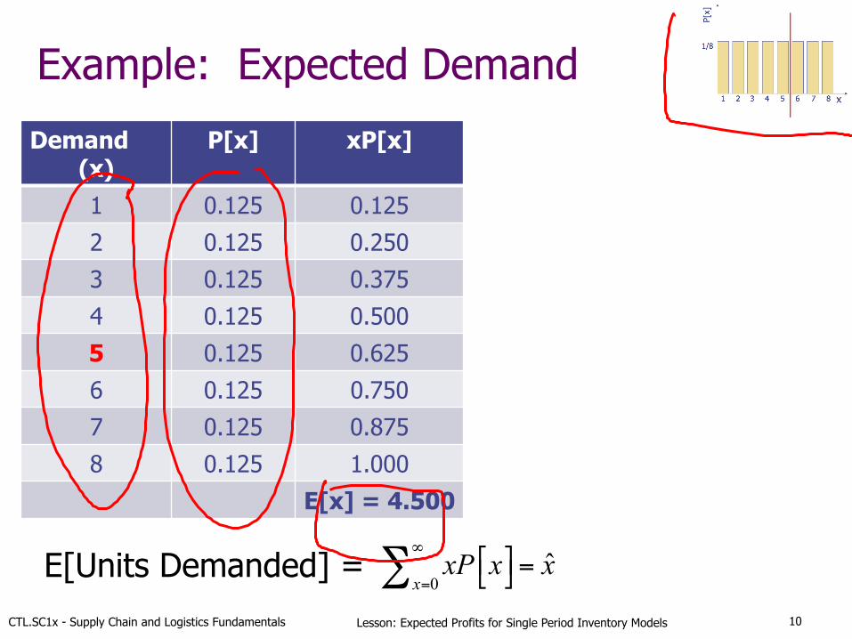
Demand (x)
P[x] xP[x]
1 0.125 0.125
2 0.125 0.250
3 0.125 0.375
4 0.125 0.500
5 0.125 0.625
6 0.125 0.750
7 0.125 0.875
8 0.125 1.000
E[x] = 4.500
Example: Expected Demand
xP x!" #$x=0
∞
∑ = x̂
10
E[Units Demanded] =
CTL.SC1x - Supply Chain and Logistics Fundamentals Lesson: Expected Profits for Single Period Inventory Models
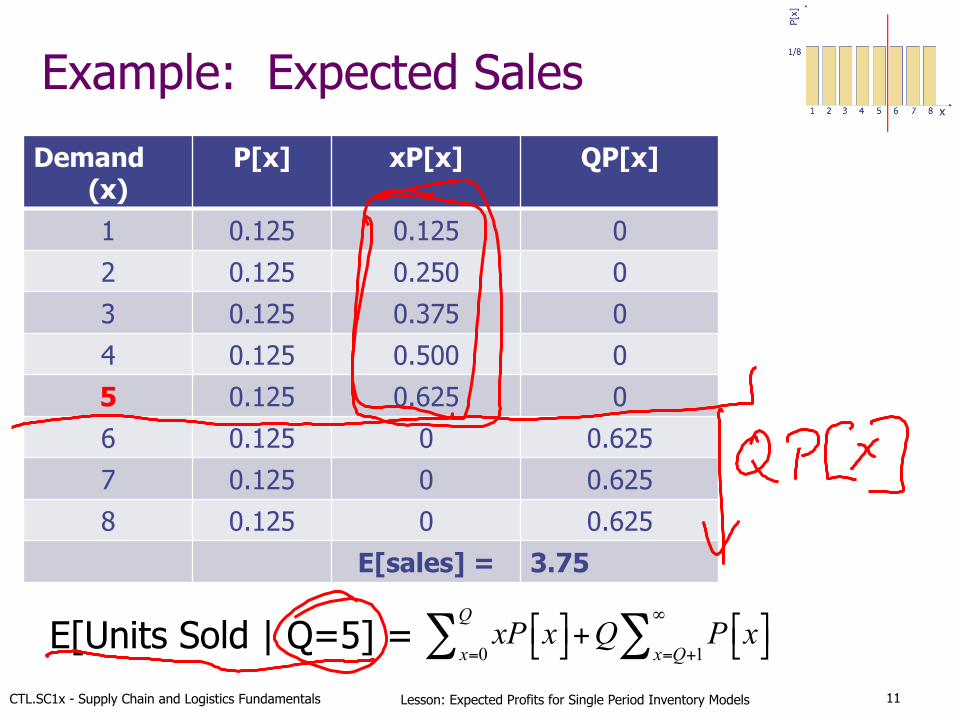
Demand (x)
P[x] xP[x] QP[x]
1 0.125 0.125 0
2 0.125 0.250 0
3 0.125 0.375 0
4 0.125 0.500 0
5 0.125 0.625 0
6 0.125 0 0.625
7 0.125 0 0.625
8 0.125 0 0.625
E[sales] = 3.75
Example: Expected Sales
xP x!" #$x=0
Q∑ +Q P x!" #$x=Q+1
∞
∑11
E[Units Sold | Q=5] =
CTL.SC1x - Supply Chain and Logistics Fundamentals Lesson: Expected Profits for Single Period Inventory Models
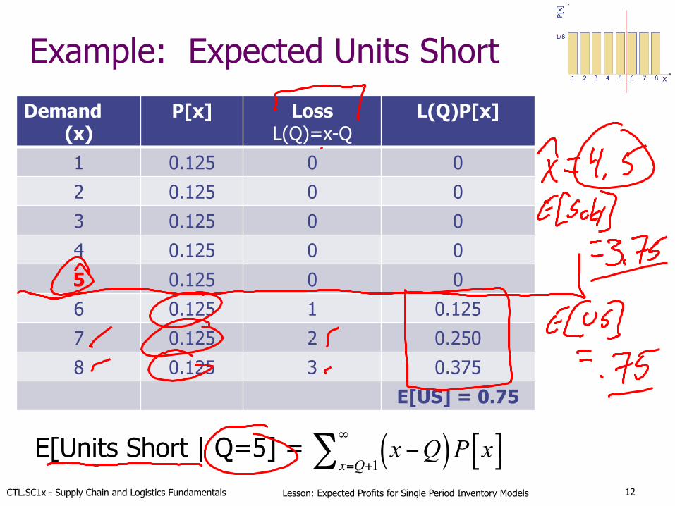
Demand (x)
P[x] Loss L(Q)=x-Q
L(Q)P[x]
1 0.125 0 0
2 0.125 0 0
3 0.125 0 0
4 0.125 0 0
5 0.125 0 0
6 0.125 1 0.125
7 0.125 2 0.250
8 0.125 3 0.375
E[US] = 0.75
Example: Expected Units Short
x −Q( )P x"# $%x=Q+1
∞
∑12
E[Units Short | Q=5] =
CTL.SC1x - Supply Chain and Logistics Fundamentals Lesson: Expected Profits for Single Period Inventory Models
Unit Normal Loss Function
13
CTL.SC1x - Supply Chain and Logistics Fundamentals Lesson: Expected Profits for Single Period Inventory Models
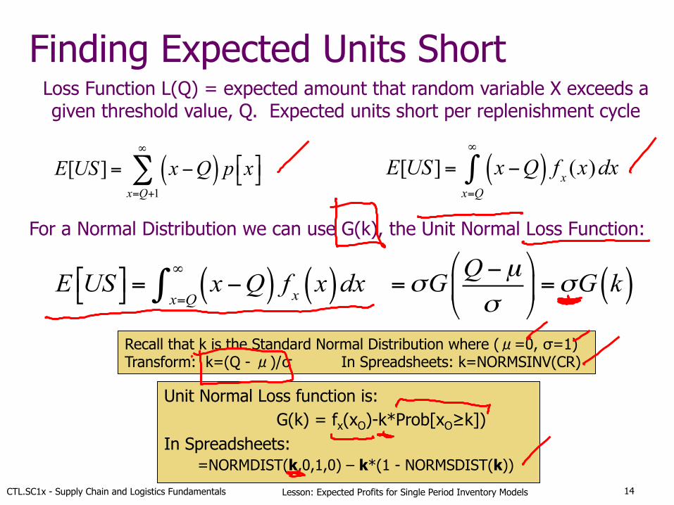
Finding Expected Units Short
E[US]= x −Q( ) p x"# $%x=Q+1
∞
∑ E[US]= x −Q( ) f x (x)dxx=Q
∞
∫
Loss Function L(Q) = expected amount that random variable X exceeds a given threshold value, Q. Expected units short per replenishment cycle
Unit Normal Loss function is: G(k) = fx(xO)-k*Prob[xO≥k])
In Spreadsheets: =NORMDIST(k,0,1,0) – k*(1 - NORMSDIST(k))
E US!" #$= x −Q( ) f x x( )dxx=Q
∞
∫ =σG Q −µσ
(
)*
+
,-=σG k( )
For a Normal Distribution we can use G(k), the Unit Normal Loss Function:
Recall that k is the Standard Normal Distribution where (μ=0, σ=1) Transform: k=(Q - μ)/σ In Spreadsheets: k=NORMSINV(CR)
14
CTL.SC1x - Supply Chain and Logistics Fundamentals Lesson: Expected Profits for Single Period Inventory Models
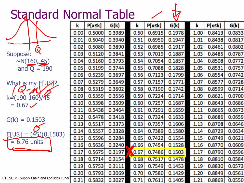
Standard Normal Table
Suppose: ~N(160, 45) and Q = 190 What is my E[US]? k=(190-160)/45 = 0.67 G(k) = 0.1503 E[US] = (45)(0.1503) = 6.76 units
15
CTL.SC1x - Supply Chain and Logistics Fundamentals Lesson: Expected Profits for Single Period Inventory Models
NFL Jersey Example Solution
16
CTL.SC1x - Supply Chain and Logistics Fundamentals Lesson: Expected Profits for Single Period Inventory Models
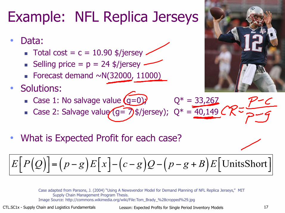
Example: NFL Replica Jerseys
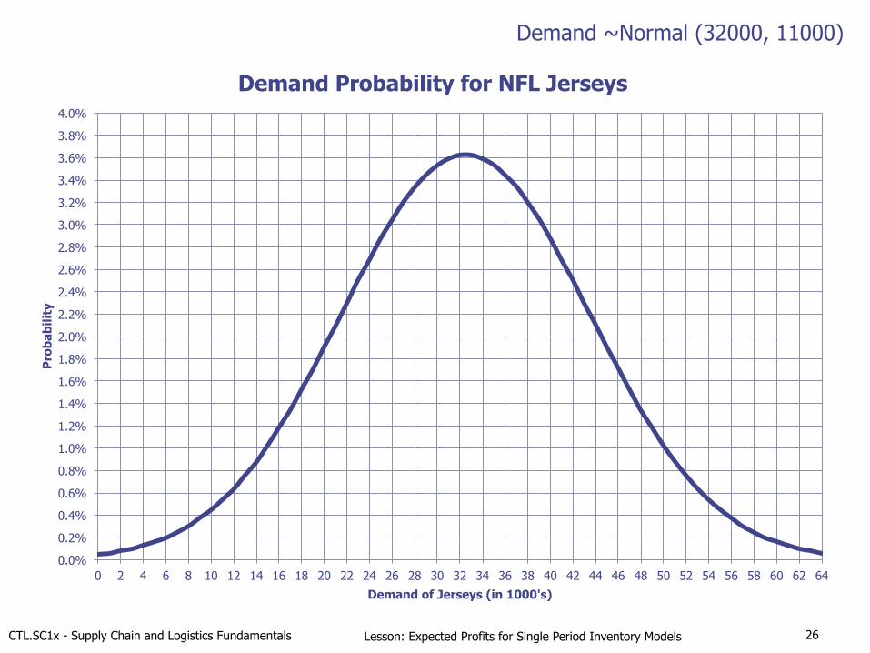
• Data: n Total cost = c = 10.90 $/jersey n Selling price = p = 24 $/jersey n Forecast demand ~N(32000, 11000)
• Solutions: n Case 1: No salvage value (g=0); Q* = 33,267 n Case 2: Salvage value (g= 7 $/jersey); Q* = 40,149
• What is Expected Profit for each case?
Case adapted from Parsons, J. (2004) “Using A Newsvendor Model for Demand Planning of NFL Replica Jerseys,” MIT Supply Chain Management Program Thesis.
Image Source: http://commons.wikimedia.org/wiki/File:Tom_Brady_%28cropped%29.jpg
E P Q( )!"
#$= p− g( )E x!" #$− c− g( )Q − p− g + B( )E UnitsShort!" #$
17
CTL.SC1x - Supply Chain and Logistics Fundamentals Lesson: Expected Profits for Single Period Inventory Models
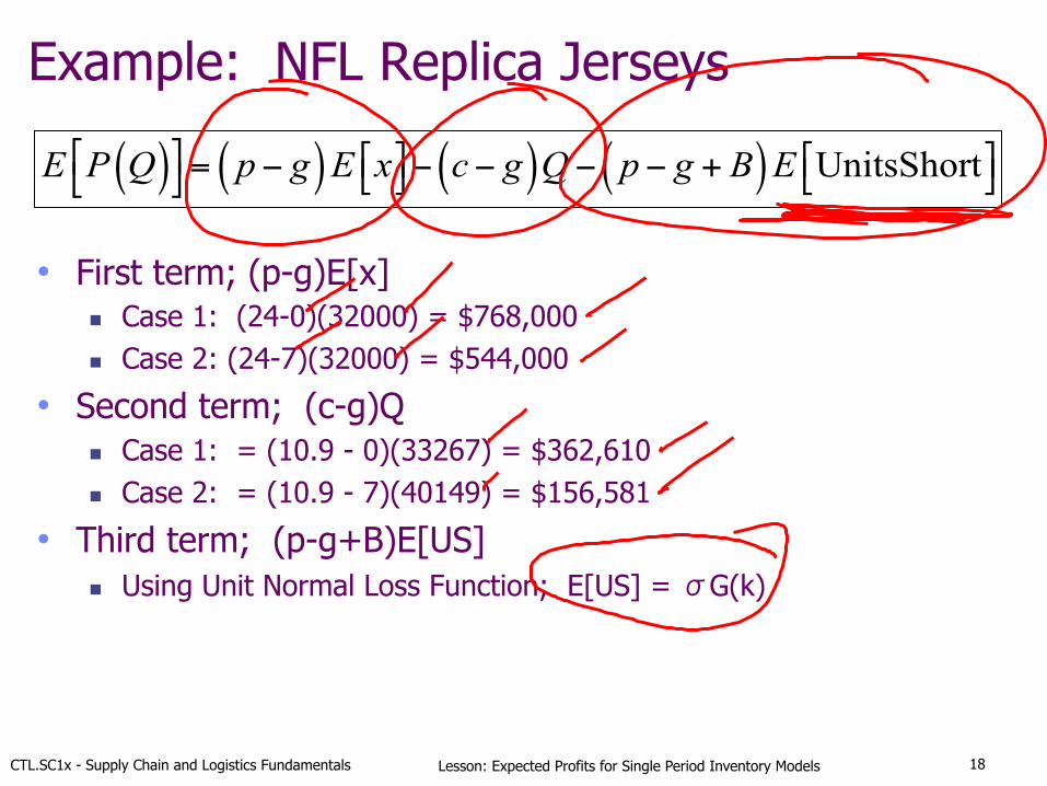
Example: NFL Replica Jerseys
• First term; (p-g)E[x] n Case 1: (24-0)(32000) = $768,000 n Case 2: (24-7)(32000) = $544,000
• Second term; (c-g)Q n Case 1: = (10.9 - 0)(33267) = $362,610 n Case 2: = (10.9 - 7)(40149) = $156,581
• Third term; (p-g+B)E[US] n Using Unit Normal Loss Function; E[US] = σG(k)
E P Q( )!"
#$= p− g( )E x!" #$− c− g( )Q − p− g + B( )E UnitsShort!" #$
18
CTL.SC1x - Supply Chain and Logistics Fundamentals Lesson: Expected Profits for Single Period Inventory Models
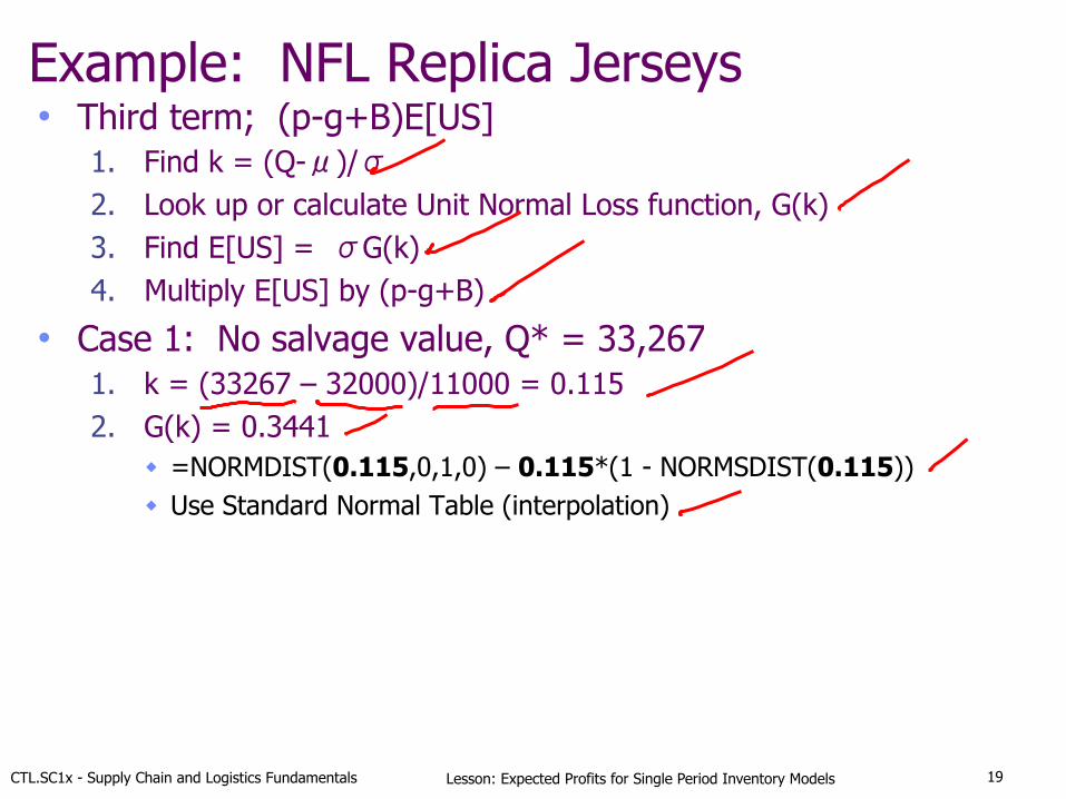
Example: NFL Replica Jerseys • Third term; (p-g+B)E[US]
1. Find k = (Q-μ)/σ 2. Look up or calculate Unit Normal Loss function, G(k) 3. Find E[US] = σG(k) 4. Multiply E[US] by (p-g+B)
• Case 1: No salvage value, Q* = 33,267 1. k = (33267 – 32000)/11000 = 0.115 2. G(k) = 0.3441
w =NORMDIST(0.115,0,1,0) – 0.115*(1 - NORMSDIST(0.115)) w Use Standard Normal Table (interpolation)
19
CTL.SC1x - Supply Chain and Logistics Fundamentals Lesson: Expected Profits for Single Period Inventory Models
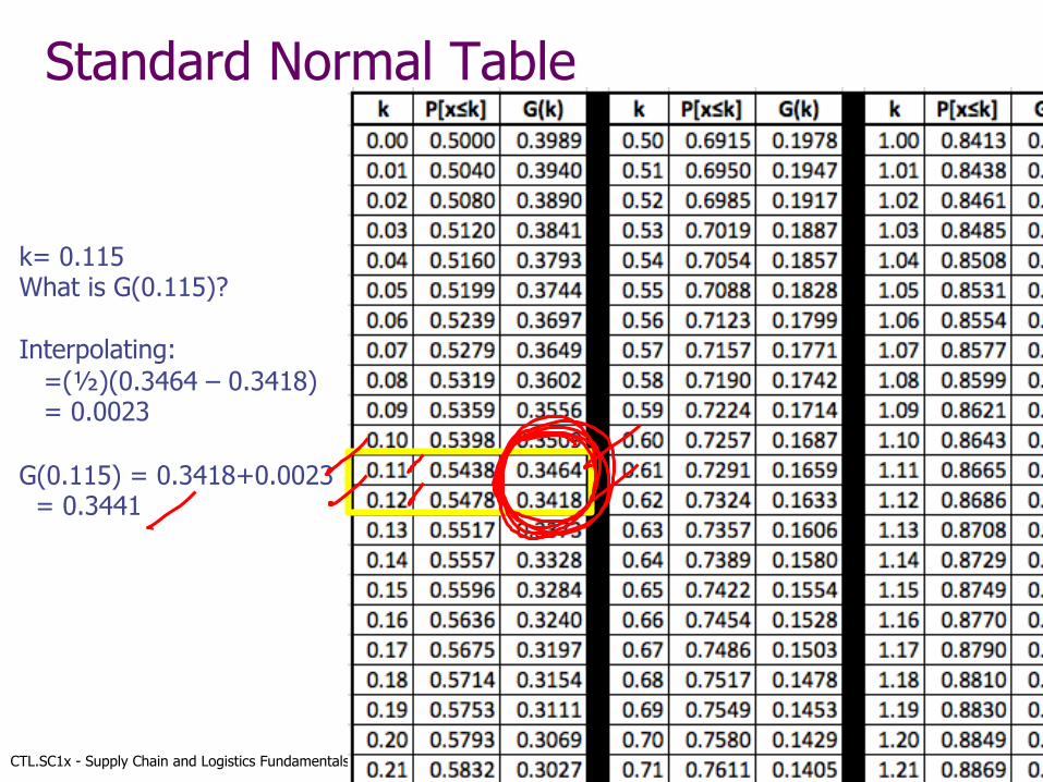
Standard Normal Table
k= 0.115 What is G(0.115)? Interpolating: =(½)(0.3464 – 0.3418) = 0.0023 G(0.115) = 0.3418+0.0023 = 0.3441
20
CTL.SC1x - Supply Chain and Logistics Fundamentals Lesson: Expected Profits for Single Period Inventory Models
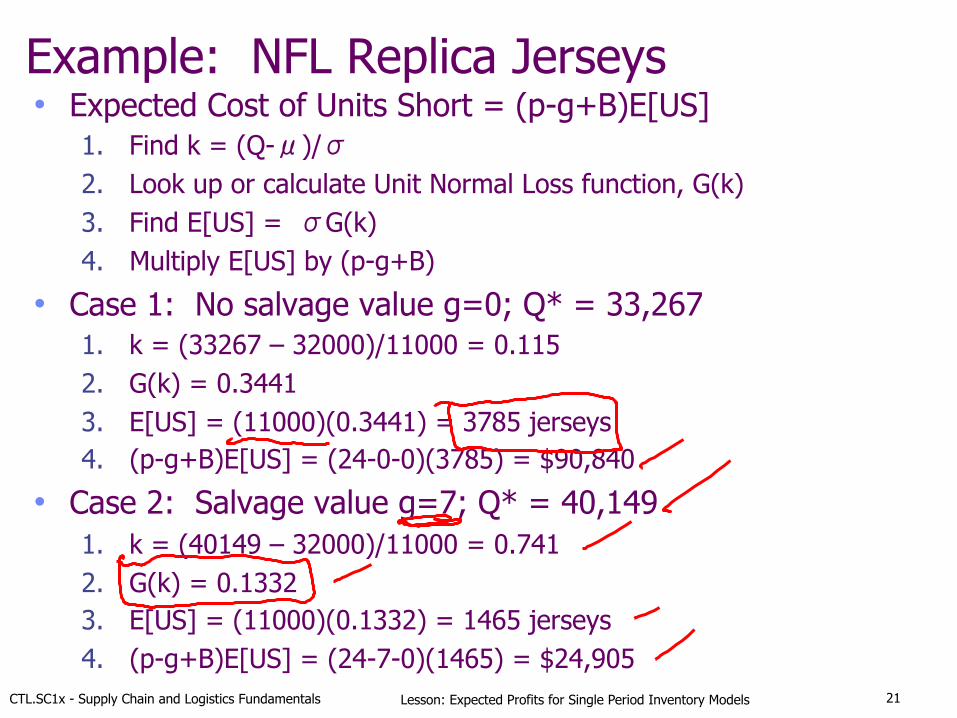
Example: NFL Replica Jerseys • Expected Cost of Units Short = (p-g+B)E[US]
1. Find k = (Q-μ)/σ 2. Look up or calculate Unit Normal Loss function, G(k) 3. Find E[US] = σG(k) 4. Multiply E[US] by (p-g+B)
• Case 1: No salvage value g=0; Q* = 33,267 1. k = (33267 – 32000)/11000 = 0.115 2. G(k) = 0.3441 3. E[US] = (11000)(0.3441) = 3785 jerseys 4. (p-g+B)E[US] = (24-0-0)(3785) = $90,840
• Case 2: Salvage value g=7; Q* = 40,149 1. k = (40149 – 32000)/11000 = 0.741 2. G(k) = 0.1332 3. E[US] = (11000)(0.1332) = 1465 jerseys 4. (p-g+B)E[US] = (24-7-0)(1465) = $24,905
21
CTL.SC1x - Supply Chain and Logistics Fundamentals Lesson: Expected Profits for Single Period Inventory Models
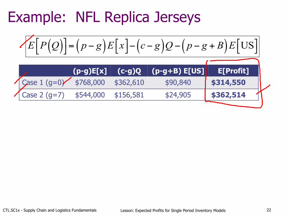
Example: NFL Replica Jerseys
(p-g)E[x] (c-g)Q (p-g+B) E[US] E[Profit]
Case 1 (g=0) $768,000 $362,610 $90,840 $314,550
Case 2 (g=7) $544,000 $156,581 $24,905 $362,514
E P Q( )!"
#$= p− g( )E x!" #$− c− g( )Q − p− g + B( )E US!" #$
22
CTL.SC1x - Supply Chain and Logistics Fundamentals Lesson: Expected Profits for Single Period Inventory Models
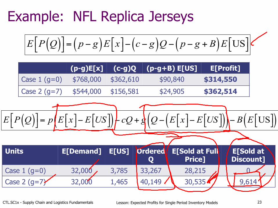
Example: NFL Replica Jerseys
(p-g)E[x] (c-g)Q (p-g+B) E[US] E[Profit]
Case 1 (g=0) $768,000 $362,610 $90,840 $314,550
Case 2 (g=7) $544,000 $156,581 $24,905 $362,514
E P Q( )!"
#$= p− g( )E x!" #$− c− g( )Q − p− g + B( )E US!" #$
Units E[Demand] E[US] Ordered Q
E[Sold at Full Price]
E[Sold at Discount]
Case 1 (g=0) 32,000 3,785 33,267 28,215 0
Case 2 (g=7) 32,000 1,465 40,149 30,535 9,614
E P Q( )!"
#$= p E x!" #$− E US!" #$( )− cQ+ g Q − E x!" #$− E US!" #$( )( )− B E US!" #$( )
23
CTL.SC1x - Supply Chain and Logistics Fundamentals Lesson: Expected Profits for Single Period Inventory Models
Key Points from Lesson
24
CTL.SC1x - Supply Chain and Logistics Fundamentals Lesson: Expected Profits for Single Period Inventory Models
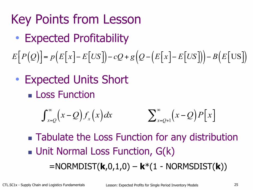
Key Points from Lesson • Expected Profitability
• Expected Units Short n Loss Function
n Tabulate the Loss Function for any distribution n Unit Normal Loss Function, G(k)
x −Q( ) f x x( )dxx=Q
∞
∫ x −Q( )P x$% &'x=Q+1
∞
∑
E P Q( )!"
#$= p E x!" #$− E US!" #$( )− cQ+ g Q − E x!" #$− E US!" #$( )( )− B E US!" #$( )
=NORMDIST(k,0,1,0) – k*(1 - NORMSDIST(k))
25
CTL.SC1x - Supply Chain and Logistics Fundamentals Lesson: Expected Profits for Single Period Inventory Models
0.0%
0.2%
0.4%
0.6%
0.8%
1.0%
1.2%
1.4%
1.6%
1.8%
2.0%
2.2%
2.4%
2.6%
2.8%
3.0%
3.2%
3.4%
3.6%
3.8%
4.0%
0 2 4 6 8 10 12 14 16 18 20 22 24 26 28 30 32 34 36 38 40 42 44 46 48 50 52 54 56 58 60 62 64
Pro
bab
ilit
y
Demand of Jerseys (in 1000's)
Demand Probability for NFL Jerseys
26
Demand ~Normal (32000, 11000)
MIT Center for Transportation & Logistics
CTL.SC1x -Supply Chain & Logistics Fundamentals
Questions, Comments, Suggestions? Use the Discussion!
Recommended