Fifth International Symposium on Marine Propulsors smp’17, Espoo, Finland, June 2017
Simulate the PPTC propeller with a vortex particle-boundary element hybrid method
Youjiang Wang1, Moustafa Abdel-Maksoud2, Peng Wang1, Baowei Song1
1School of Marine Science and Technology, Northwestern Polytechnical University, Xi’an, P.R. China
2Institute for Fluid Dynamics and Ship Theory, Hamburg University of Technology, Hamburg, Germany
ABSTRACT
To investigate the possibility of using VPM in the marine
propeller flow simulation, this work applies a hybrid
method coupling the boundary element method and the
vortex particle method to analyze the flow around the
Potsdam Propeller Test Case (PPTC) propeller. The
boundary element method is used to model the blade
surface while the vortex particle method is used for the
wake flow field. The results show that the open water
characteristics obtained with the developed hybrid method
correlate very well with the experimental result. The
obtained tip vortex position and velocity distribution also
correlates well with the experimental measurement
qualitatively. The computational time is also presented
and compared with other methods.
Keywords
marine propeller, vortex particle method, BEM-VPM
hybrid method.
1 INTRODUCTION
For the analysis of noise, interaction and off-design
working conditions of the marine propeller, it is always
essential to get the accurate prediction of the flow details,
especially the vortex structures in the flow. Existing
technique includes using RANS or DES solver to solve
the flow detail, which is quite successful in recent years.
Besides, to predict the leading edge vortex and tip vortex
efficiently, Tian & Kinnas (2015) presented a VIScous
Viscosity Equation solver, in which the concentration of
vorticity is exploited and the viscous vorticity equation is
solved with finite volume method in a small region
around the propeller blade. Far downstream vortex wake
is modeled with potential wakes and velocity boundary
condition is utilized to consider the mutual influence. The
current work is aimed to investigate the possibility of
applying vortex particle method (VPM) in the simulation
of the flow around marine propellers.
The VPM is a scheme designed especially for the vortex
analysis. It is based on the Lagrangian discretization of
the vorticity transport equation. The vorticity field is
discretized with a set of Lagrangian vortex particles. The
particles carry the vorticity, move with the field velocity
and only exist in the region where the vorticity is not
negligible. The Lagrangian discretization makes VPM
free from the numerical diffusion, which is always
suffered by the grid-based solvers.
Because of the advantages of VPM in the vortex
simulation, it has been adopted for various simulations
relating to vortices. Mammetti et al (1999) adopted VPM
to study the collision of a vortex ring with a solid wall for
the investigation of the artificial noise. The obtained
numerical vortex structure agreed very well with the
experimental visualization. The instability of two pairs of
counter rotating vortices in the aircraft wake has been
simulated using VPM by Chatelain et al (2008). The -
shape loops formed by the main and secondary vortices,
which is typical in the medium wavelength instability,
have been reproduced in simulation, and the evolution of
longitudinal energy modes (along the stream-wise
direction) correlated well with those observed in
experiments. VPM has also been used to model the wake
field of wind turbine by Chatelain et al (2011), Backaert
et al (2015), and Branlard et al (2016). In their works, the
wind turbine blades are modeled with lifting lines and the
shedding vorticity is modeled with vortex particles.
However, VPM has not yet been used to analyze the flow
around marine propellers.
VPM is to be applied for the simulation of marine
propeller flow in this work. Because of the complexity of
handling the boundary condition in VPM, in the current
work it is coupled with the boundary element method
(BEM). In the hybrid method BEM is used to model the
blade surface and VPM is used to model the wake flow.
BEM and VPM are described briefly in the following
section. The coupling scheme is introduced in section 3.
In section 4, the hybrid method is used to analyze the
PPTC propeller and the results are given. In section 5, the
main conclusions of the current work are stated.
2 EXISTING METHODS
3.1 Boundary Element Method
In the current work, a low order in-house BEM code is
adopted. In the BEM code, the field velocity consists of
the free stream velocity and the disturbed velocity. The
disturbed velocity is induced by the singularities on the
body surface and the wake surface. The singularities on

the body panels are dipole and source, while on the wake
panels there is only dipole, as shown in Figure 1. The
strengths of the singularities are determined with the
boundary conditions stating that the disturbed potential
inside the body surface is zero.
On the body surface, the tangential component of the
disturbed velocity is obtained by evaluating the disturbed
potential’s surface gradient. The pressure is computed
according to the Bernoulli equation. The viscous force is
evaluated using an empirical formula which relates the
viscous shear stress to local Reynolds number and
velocity, i.e.
0.5f p fS CF u u (1)
where Ff is the viscous force acting on a panel, Sp is the
area of the panel, is the water density, u is the total
relative fluid velocity on the panel and Cf is the friction
coefficient. According to Schlichting (1987), Cf can be
evaluated as
2.3
10(log Re 0.65)fC (2)
where Re is the local Reynolds number on the panel.
Figure 1 The distribution of singularities in the adopted in-
house BEM code.
With the pressure and viscous force, the thrust and torque
of the propeller can be obtained.
For the unsteady case, the wake panels are moved with
the total field velocity. For the steady case, the wake is
aligned with a faster algorithm, i.e., the DAM scheme
stated in Wang et al (2016a).
For more details about the BEM code, please refer to
Wang et al (2016a), Wang et al (2016b), and Wang et al
(2017a).
3.2 Vortex Particle Method
The VPM is based on the vorticity transport equation (or
the vorticity-velocity formation of the NS equation),
which is
D( )
Dt
ωu ω (3)
where t is the time, u is the velocity, v is the kinematic
viscosity and ω = u is the vorticity. The vorticity
field is discretized with a set of Lagrangian vector –
valued particles, i.e.
( ) ( )p p
p
x ω x x (4)
where xp and ap represent the positions and strengths of
particles, respectively, and stands for the mollification
function which depends on the particle’s core size . The
mollification function is defined as
3
1 | |( ) ( )e
xx . (5)
In this work, the Gaussian mollification function is
adopted for , i.e.
2
3/ 2
1( ) exp( )
2(2 )
. (6)
The particle strength is the total vorticity contained in the
particle’s volume, i.e.
dp
pV
V (7)
where Vp denotes the volume associated with the particle
p.
Discretize the vorticity transport equation with vortex
particles, the formulas governing the VPM simulation are
obtained as
d( )
d
p
put
xx (8)
d( ) ( )
d
p
p p p pVt
u x x
(9)
In Equation (9), u is called the vorticity stretching
term while V is called the viscous diffusion term.
The local velocity u consists of the free stream velocity
and the disturbed velocity. The disturbed velocity is the
summation of the induced velocity from every vortex
particle as follows
( ) ( )i p p
p
u x K x x (10)
where Kis the velocity kernel, which is obtained by
applying the Biot-Savart theory to the mollified vortex
particle. The gradient of the velocity is
( ) ( )i p p
p
u x K x x . (11)
The viscous diffusion term (especially the Laplacian
operator ) cannot be evaluated directly in the particle
system. In the current work, the particle strength
exchange technique developed by Degond & Mas-Gallic
(1989) is adopted for the relative calculation.
As the simulation advances, the flow’s local strain always
leads to particles clustering in one direction and spreading
in other directions. The non-uniform distribution may

endanger the convergence and stability of VPM. Thus, it
is necessary to redistribute the vortex particles to regular
positions. In the current work, the 3D interpolation using
the Cartesian product of M4’ function is adopted to obtain
the strengths of the new particles.
In the engineering related applications, the inter-particle
spacing may not be small enough to capture all the
turbulence scales. In such cases, sub-grid scale dissipation
model is needed to consider the influence of the under-
resolved scale dissipation. In the current work, the
artificial viscosity model promoted by Cottet (1996)
especially for VPM is adopted.
For more details about the VPM, please refer to Wang et
al (2017b), Cottet & Koumoutsakos (2000), and
Ploumhans et al (2002).
3 THE HYBRID METHOD
3.2 Coupling Scheme
The current work couples the BEM and VPM together to
calculate the marine propeller flow, as shown in Figure 2.
The BEM is used to model the propeller surface and the
VPM is used to model the wake flow. Two columns of
wake panels are left as the buffer wake.
The buffer wake is used to connect the BEM and VPM
systems. In the BEM system, the buffer wake is used to
satisfy the Kutta condition and close the equation system.
In each time step, a new column of wake panels are shed
from the trailing edge and the last column are converted
to vortex particles. The conversion is based on the
relationship between dipole distribution and vorticity,
s n (12)
where is the dipole strength on the panel, n is the unit
normal vector and s denotes the surface gradient on the
panel. In the low order panel method, the dipole strength
is constant on one wake panel, which means the vorticity
strength obtained with Equation (12) is zero. In the
current work, the dipole strength on a panel is regarded as
the value at the panel’s center, and 2D interpolation is
applied to construct a continuous non-constant
distribution of the dipole strength on the wake surface.
To consider the influence of the VPM system on the BEM
system, the vortex particles’ induced velocities on the
body panels are calculated. These velocities are regarded
as a part of the free stream velocity when the source
strengths are evaluated and as a part of the disturbed
velocity when the pressure is evaluated. In the movement
of the buffer wake panels, the vortex particles’ induced
velocity is also included in the total field velocity.
To consider the influence of the BEM system on the VPM
system, the panels’ induced velocities at the particles’
positions are evaluated and regarded as free stream
velocity. At the same time, the gradients of the induced
velocities are also evaluated for the computation of the
vorticity stretching term.
3.2 Rotational Periodic Boundary
For the simulation of propellers, to reduce the
computational time, only a subdomain corresponding to
one blade is modeled. The rest are modeled with the
rotational periodic boundary condition. As particles move
out the subdomain from one periodic boundary,
corresponding new ones are created and come in from the
other periodic boundary. When the induced velocities are
computed, the contribution of the rest domain is included
by creating virtual particles according to the periodic
condition.
The cross-section of the modeled subdomain is a sector.
For the particle redistribution, regular hexahedral cells are
generated in the modeled subdomain and new particles
are placed at the cell centers. The inter-particle spacing h
is utilized to control the particle density. Along the axial
and radial directions, uniform grids with space being h are
used. Every radial strip is divided to a specific number of
uniform cells so that the cell’s tangential length is around
h, as shown Figure 3.
In the coupling method, to avoid particle piercing into the
body, the particle redistribution is not carried out for the
whole domain, but for the domain after a certain position.
Such a treatment can also help reduce particle number and
save computational time.
Figure 2 Different computational elements in the vortex
particle-boundary element hybrid method.
Figure 3 The uniform particle distribution on the sector-shape
cross section.

4 NUMERICAL RESULTS
The open water characteristics of the PPTC propeller are
evaluated using BEM and the hybrid method,
respectively. The orthogonal panel arrangement is used on
the propeller blade, as shown in Figure 4. The panel
numbers along the chordwise and radial direction are 60
and 25, respectively. The time step is set so that the
propeller rotates 6 degrees every step. The geometry of
the PPTC propeller is given in Heinke (2011).
In the hybrid method, the particle’s core size determines
the range in which the particle distributes its vorticity. For
the propeller wake, it is assumed that such a range
approximately equal to the boundary layer thickness near
the trailing edge. In this work, the particle core size is
set around the boundary layer thickness at r/R=0.7, which
is evaluated according to Schlichting (1987) as
1/70.154 Re C (13)
where Re is the local Reynolds number and C is the chord
length. The inter-particle spacing h is set to be 1.2.
In the simulation, the particle redistribution beginning
position is 0.4D after the propeller disk, where D denotes
the propeller’s diameter. To control the increase of
particle number, the particle will be deleted when it goes
further than 1.5D after the propeller disk. To achieve the
convergent results, 300 steps are simulated from the
beginning without any wake panels and vortex particles.
The convergence history of the thrust and torque
coefficient for the case with J=1.0 are shown in Figure 5.
The particles distributions during the calculation and in
the final step are given in Figure 6. It can be concluded
that 300 steps are enough to obtain the final convergent
result.
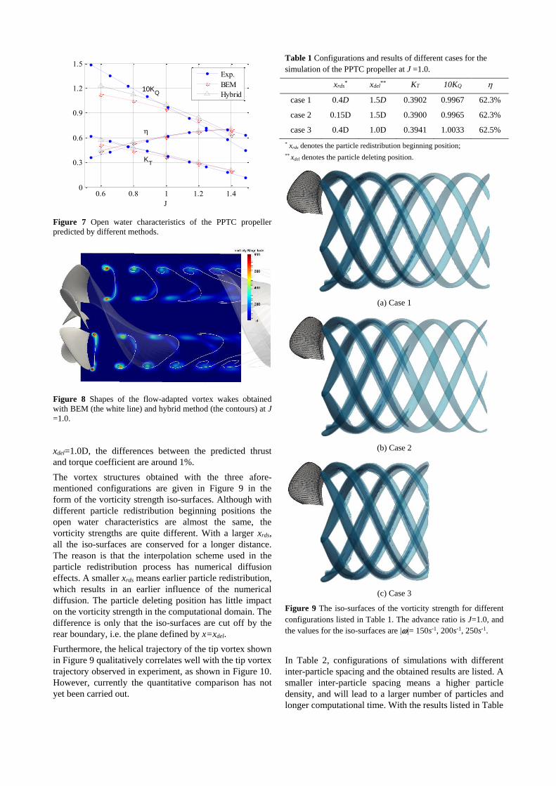
The obtained open water characteristics are given in
Figure 7 together with the experimental result. The
prediction of the hybrid method is more accurate than that
of BEM, especially for low advance ratios. This is
because the hybrid method models the wake flow more
physically, which takes consideration of the shedding
wake’s thickness and the viscous diffusion. Figure 8
shows the comparison between the shapes of the vortex
wakes obtained with BEM and hybrid method at J =1.0.
Obvious differences are observed in the inner region. The
vortex wake obtained with BEM is located further to the
downstream. The different wake shapes then lead to
different open water characteristics.
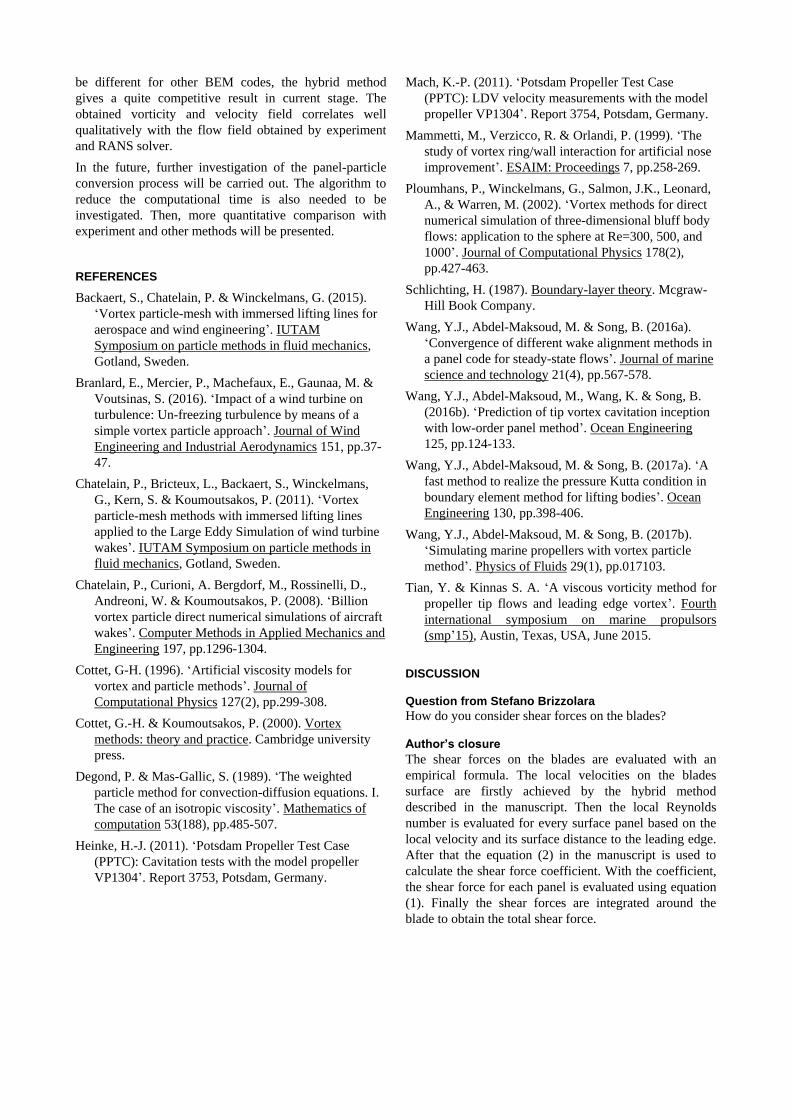
To investigate the influence of the particle redistribution
beginning position and the particle deleting position on
the predicted open water performance and the wake flow
detail, three simulations with different configurations are
carried out with the hybrid method for the PPTC propeller
at J=1.0. The configurations are listed in Table 1, where
the obtained open water characteristics are also given.
The particle redistribution beginning position xrds has little
effect on the predicted open water performance. The
difference is less than 0.1%. The particle deleting position
xdel (or the computational domain’s length) has a much
larger influence. For the two cases with xdel=1.5D and
Figure 4 The panel arrangement on the propeller blade.
0 50 100 150 200 250 3000.38
0.4
0.42
0.44
KT
0 50 100 150 200 250 3000.095
0.1
0.105
0.11K
Q
steps
Figure 5 Convergence history of the thrust coefficient and
torque coefficient in the hybrid method (for PPTC propeller at
J=1.0).
(a) 48th step
(b) 300th step
Figure 6 Particle distributions during the calculation. The color
is defined by the particle’s strength magnitude (for PPTC
propeller at J=1.0).
0.6 0.8 1 1.2 1.40
0.3
0.6
0.9
1.2
1.5
J
Exp.
BEM
Hybrid10K
Q
KT
Figure 7 Open water characteristics of the PPTC propeller
predicted by different methods.
Figure 8 Shapes of the flow-adapted vortex wakes obtained
with BEM (the white line) and hybrid method (the contours) at J
=1.0.
xdel=1.0D, the differences between the predicted thrust
and torque coefficient are around 1%.
The vortex structures obtained with the three afore-
mentioned configurations are given in Figure 9 in the
form of the vorticity strength iso-surfaces. Although with
different particle redistribution beginning positions the
open water characteristics are almost the same, the
vorticity strengths are quite different. With a larger xrds,
all the iso-surfaces are conserved for a longer distance.
The reason is that the interpolation scheme used in the
particle redistribution process has numerical diffusion
effects. A smaller xrds means earlier particle redistribution,
which results in an earlier influence of the numerical
diffusion. The particle deleting position has little impact
on the vorticity strength in the computational domain. The
difference is only that the iso-surfaces are cut off by the
rear boundary, i.e. the plane defined by x=xdel.
Furthermore, the helical trajectory of the tip vortex shown
in Figure 9 qualitatively correlates well with the tip vortex
trajectory observed in experiment, as shown in Figure 10.
However, currently the quantitative comparison has not
yet been carried out.
Table 1 Configurations and results of different cases for the
simulation of the PPTC propeller at J =1.0.
xrds* xdel
** KT 10KQ
case 1 0.4D 1.5D 0.3902 0.9967 62.3%
case 2 0.15D 1.5D 0.3900 0.9965 62.3%
case 3 0.4D 1.0D 0.3941 1.0033 62.5%
* xrds denotes the particle redistribution beginning position;
** xdel denotes the particle deleting position.
(a) Case 1
(b) Case 2
(c) Case 3
Figure 9 The iso-surfaces of the vorticity strength for different
configurations listed in Table 1. The advance ratio is J=1.0, and
the values for the iso-surfaces are ||= 150s-1, 200s-1, 250s-1.
In Table 2, configurations of simulations with different
inter-particle spacing and the obtained results are listed. A
smaller inter-particle spacing means a higher particle
density, and will lead to a larger number of particles and
longer computational time. With the results listed in Table

Figure 10 Experimental observation of the tip vortex cavitation,
which reflects the trajectory of the tip vortex (taken from Heinke
(2011)).
2, it can be found that increasing the inter-particle spacing
will cause an decrease in KT and KQ, however, the
differences are quite small (less than 0.3%). Thus, the
inter-particle spacing (or particle number) has little
influence, if any, on the predicted KT and KQ.
However, the inter-particle spacing has a noticeable
influence on the vorticity strength, as shown in Figure 11.
A smaller inter-particle spacing leads to a stronger
vorticity in the wake flow field. Actually, the voriticy
strength is directly affected by the particle core size , which determines the range of the vorticity distribution.
Such a range should be correlated to the boundary layer
thickness, as given by Equation (13).
Table 2 Results of the simulations with different inter-particle
spacing h for PPTC propeller at J =1.0.
h KT 10KQ Tstep*
case 1 0.01D 0.011D 0.3902 0.9967 62.3% 181s
case 2 0.015D 0.016D 0.3895 0.9948 62.3% 30s
case 3 0.02D 0.021D 0.3890 0.9937 62.3% 15s
* Tstep denotes the averaged computational time for every step.
The flow around PPTC propeller has also been simulated
with the commercial RANS solver CFX. In the
simulation, the rotational periodic boundary condition is
used and only one blade is simulated. The whole
computational domain consists of a rotational domain
surrounding the blade and a static outer domain. For the
rotational domain 802K hexahedral cells are used and for
the static domain 523K cells are used. The k- SST
model is adopted for the turbulence model. 500 steps are
simulated to achieve the final convergent result.
Vortex structures obtained with CFX and the hybrid
method are given in Figure 12. The hybrid method leads
to thinner iso-surfaces, which means at the beginning
position the vorticity strength is smaller than that obtained
with CFX. This may results from the too large particle
core size used in the panel-to-particle conversion process.
(a) Case 1, h=0.011D
(b) Case 2, h=0.016D
(c) Case 3, h=0.021D
Figure 11 The vorticity strength on the plane located 0.16D
after the propeller disk obtained by different simulations listed
in Table 2 (the advance ratio is J =1.0).
Further investigation of the conversion process will
probably improve the correlation. In addition, the radius
of iso-surfaces obtained with the hybrid method decreases

much slower, which means the hybrid method has a better
ability to conserve the vorticity than the RANS solver, at
least with current configurations. Besides, the iso-surfaces
obtained with CFX are discontinuous near the interface
while those obtained with the hybrid method are
continuous and smooth.
The distribution of the axial velocity on the plane located
0.2D after the propeller disk is given in Figure 13 together
with the experimental measurement by Mach (2011). The
tip vortex positions correlate very well. The small inward
offset is because that in BEM 1% of the blade is cut out at
the tip. The velocity gradient obtained with the hybrid
method is smaller than that observed in the experiment.
This indicates that with the current configuration, the
calculated concentration of the vorticity is not enough. To
obtain a more accurate prediction of the velocity field, a
higher particle density is needed.
The computational time of different methods is listed in
Table 3. The current hybrid method is not a time-saving
method. However, the particle density does not influence
the predicted open water characteristics very much. A
larger inter-particle spacing could reduce the total
simulation time within 2 hours. On the other side, a more
accurate prediction of the flow detail needs a smaller
inter-particle spacing and more computational time.
Furthermore, the algorithm to improve the computational
efficiency is also under research.
Table 3 The computational time for different methods.
Total Time Steps Averaged time per step
Hybrid Method 15.1h 300 181s
BEM 74.0s 9 8.24s
CFX 4.72h 500 34s
(a) CFX (b) Hybrid method
Figure 12 Comparison between CFX result and Coupling
method. The advance ratio is J=1.0, and the values for the iso-
surfaces are ||= 500s-1, 550s-1, 600s-1.
(a) Experimental measurement (taken from Mach (2011)).
(b) Obtained with the hybrid method.
Figure 13 The distribution of non-dimensional axial velocity on
the plane located 0.2D after the propeller disk. The velocity is
nondimensionalized by the propeller’s advance velocity Va.
4 CONCLUSIONS
In this work, a hybrid method combining the boundary
element method and the vortex particle method is used to
simulate the flow around the PPTC propeller. The blade
surface and non-penetrating boundary condition is
modeled by boundary element method, while the vortex
wake is modeled by viscous vortex particle method.
The results obtained with the hybrid method are
encouraging. The obtained thrust and torque coefficient
are more accurate than our in-house BEM code. Although
the relative merit between hybrid method and BEM may
be different for other BEM codes, the hybrid method
gives a quite competitive result in current stage. The
obtained vorticity and velocity field correlates well
qualitatively with the flow field obtained by experiment
and RANS solver.
In the future, further investigation of the panel-particle
conversion process will be carried out. The algorithm to
reduce the computational time is also needed to be
investigated. Then, more quantitative comparison with
experiment and other methods will be presented.
REFERENCES
Backaert, S., Chatelain, P. & Winckelmans, G. (2015).
‘Vortex particle-mesh with immersed lifting lines for
aerospace and wind engineering’. IUTAM
Symposium on particle methods in fluid mechanics,
Gotland, Sweden.
Branlard, E., Mercier, P., Machefaux, E., Gaunaa, M. &
Voutsinas, S. (2016). ‘Impact of a wind turbine on
turbulence: Un-freezing turbulence by means of a
simple vortex particle approach’. Journal of Wind
Engineering and Industrial Aerodynamics 151, pp.37-
47.
Chatelain, P., Bricteux, L., Backaert, S., Winckelmans,
G., Kern, S. & Koumoutsakos, P. (2011). ‘Vortex
particle-mesh methods with immersed lifting lines
applied to the Large Eddy Simulation of wind turbine
wakes’. IUTAM Symposium on particle methods in
fluid mechanics, Gotland, Sweden.
Chatelain, P., Curioni, A. Bergdorf, M., Rossinelli, D.,
Andreoni, W. & Koumoutsakos, P. (2008). ‘Billion
vortex particle direct numerical simulations of aircraft
wakes’. Computer Methods in Applied Mechanics and
Engineering 197, pp.1296-1304.
Cottet, G-H. (1996). ‘Artificial viscosity models for
vortex and particle methods’. Journal of
Computational Physics 127(2), pp.299-308.
Cottet, G.-H. & Koumoutsakos, P. (2000). Vortex
methods: theory and practice. Cambridge university
press.
Degond, P. & Mas-Gallic, S. (1989). ‘The weighted
particle method for convection-diffusion equations. I.
The case of an isotropic viscosity’. Mathematics of
computation 53(188), pp.485-507.
Heinke, H.-J. (2011). ‘Potsdam Propeller Test Case
(PPTC): Cavitation tests with the model propeller
VP1304’. Report 3753, Potsdam, Germany.
Mach, K.-P. (2011). ‘Potsdam Propeller Test Case
(PPTC): LDV velocity measurements with the model
propeller VP1304’. Report 3754, Potsdam, Germany.
Mammetti, M., Verzicco, R. & Orlandi, P. (1999). ‘The
study of vortex ring/wall interaction for artificial nose
improvement’. ESAIM: Proceedings 7, pp.258-269.
Ploumhans, P., Winckelmans, G., Salmon, J.K., Leonard,
A., & Warren, M. (2002). ‘Vortex methods for direct
numerical simulation of three-dimensional bluff body
flows: application to the sphere at Re=300, 500, and
1000’. Journal of Computational Physics 178(2),
pp.427-463.
Schlichting, H. (1987). Boundary-layer theory. Mcgraw-
Hill Book Company.
Wang, Y.J., Abdel-Maksoud, M. & Song, B. (2016a).
‘Convergence of different wake alignment methods in
a panel code for steady-state flows’. Journal of marine
science and technology 21(4), pp.567-578.
Wang, Y.J., Abdel-Maksoud, M., Wang, K. & Song, B.
(2016b). ‘Prediction of tip vortex cavitation inception
with low-order panel method’. Ocean Engineering
125, pp.124-133.
Wang, Y.J., Abdel-Maksoud, M. & Song, B. (2017a). ‘A
fast method to realize the pressure Kutta condition in
boundary element method for lifting bodies’. Ocean
Engineering 130, pp.398-406.
Wang, Y.J., Abdel-Maksoud, M. & Song, B. (2017b).
‘Simulating marine propellers with vortex particle
method’. Physics of Fluids 29(1), pp.017103.
Tian, Y. & Kinnas S. A. ‘A viscous vorticity method for
propeller tip flows and leading edge vortex’. Fourth
international symposium on marine propulsors
(smp’15), Austin, Texas, USA, June 2015.
DISCUSSION Question from Stefano Brizzolara
How do you consider shear forces on the blades? Author’s closure
The shear forces on the blades are evaluated with an
empirical formula. The local velocities on the blades
surface are firstly achieved by the hybrid method
described in the manuscript. Then the local Reynolds
number is evaluated for every surface panel based on the
local velocity and its surface distance to the leading edge.
After that the equation (2) in the manuscript is used to
calculate the shear force coefficient. With the coefficient,
the shear force for each panel is evaluated using equation
(1). Finally the shear forces are integrated around the
blade to obtain the total shear force.
Recommended