Simulations of Computing by Self-Assembly
Erik Winfree
California Institute of Technology
May 31, 1998
Abstract Winfree (1996) proposed a Turing-universal model of DNA self-assembly.
In this abstract model, DNA double-crossover molecules self-assemble to form an
algorithmically-patterned two-dimensional lattice. Here, we develop a more realistic
model based on the thermodynamics and kinetics of oligonucleotide hydridization.
Using a computer simulation, we investigate what physical factors in uence the error
rates, i.e., when the more realistic model deviates from the ideal of the abstract model.
We �nd, in agreement with rules of thumb for crystal growth, that the lowest error
rates occur at the melting temperature when crystal growth is slowest, and that error
rates can be made arbitrarily low by decreasing concentration and increasing binding
strengths.
1 Introduction
Early work in DNA computing (Adleman 1994; Lipton 1995; Boneh et al. 1996; Ouyang et al.
1997) showed how computations can be accomplished by �rst creating a combinatorial library
of DNA and then, through successive application of standard molecular biology techniques,
�ltering the library to identify the DNA representing the answer to the mathematical question.
In these approaches, the problem to be solved determines the sequence of laboratory operations
to be performed; the length of this sequence grows with problem size, intimidating many exper-
imental researchers. Consequently, a few researchers have begun looking into chemical systems
capable of performing many logical steps in a single reaction, thus leading to paradigms for
DNA computing where the problem to be solved is encoded strictly in DNA sequence; a �xed
sequence of laboratory operations is performed to determine the answer to the posed question.
Promising approaches include techniques based on PCR-like reactions (Hagiya et al. in press;
Sakamoto et al. in press ; Hartemink and Gi�ord in press; Winfree in press ) and techniques
based on DNA self-assembly (Winfree 1996; Winfree et al. in press; Jonoska et al. in press).
Although there has been experimental work exploring all these models, typically only a few
logical operations have been demonstrated. It is at this point unclear how well any of the
techniques can be scaled up. Short of full experimental demonstration, realistic simulations of
the chemical kinetics and thermodynamics can shed light on what can be expected of these
1
systems, and can point to parameter regimes where the experiments are most likely to succeed.
This paper presents a preliminary analysis of the self-assembly model of Winfree (1996).
To motivate the self-assembly model, we consider the physical process of crystallization. During
crystal growth, monomer units are added one-by-one at well-de�ned sites on the surface of the
crystal. There may be more than one type of monomer, in which case there may be several
di�erent types of binding site, each with a�nity for a di�erent monomer; typically a periodic
arrangement of units results. The question of whether periodic lattices will necessarily result
has been studied in mathematics in the context of two-dimensional tilings (Gr�unbaum and
Shephard 1986). A set of geometrical shapes (the tiles) are said to tile the plane if the tiles can
be arranged, non-overlapping, such that every point in the plane is covered. A surprising result
in the theory of tilings is that there exist sets of tiles which admit only aperiodic tilings (Berger
1966; Robinson 1971), the most elegant being the rhombs of Penrose (1978). The variety of
aperiodic patterns is limitless: using square tiles with modi�ed edges, the time-space history of
any Turing Machine can be reproduced by the tiling pattern1 (Wang 1963; Robinson 1971). Is
it possible to translate these results back to a physical system, to produce aperiodic crystals,
or even crystals which \compute"? Already, there is an extensive literature on \quasicrystals"
(Steinhardt and Ostlund 1987), materials which exhibit \prohibited" 5-fold symmetry and
which are thought to be related to the aperiodic Penrose tiles. The purpose of this paper is to
examine the suggestion in Winfree (1996) that DNA double-crossover molecules can be used to
make programmable \molecular Wang tiles" that will self-assemble into a 2D sheet to simulate
any chosen cellular automaton. It has already been shown experimentally that double-crossover
molecules can be designed to assemble into a periodic 2D sheet (Winfree et al. 1998) and that
a single logical step can proceed in a model system. In this paper we argue that it is physically
plausible to perform Turing-universal computation by crystallization.
2 An Abstract Model of 2D Self-Assembly
The results in the theory of tilings are entirely existential, saying nothing about how a correct
tiling is to be found. What is missing is a mechanism for producing tilings. In this section
we describe the relation of computation and self-assembly by presenting an abstract model of
two-dimensional (2D) self-assembly, which we call the Tile Assembly Model. The fundamental
units in this model are unit square tiles (also called monomers) with labelled edges. We have
an unlimited supply of tiles of each type. Aggregates are formed by placing new tiles next to
and aligned with existing ones such that su�ciently many of their edges have matching labels.
Tiles cannot be rotated or re ected. To de�ne the model completely, we must be precise about
when \su�ciently many" edges match. Each edge label �i has an associated strength gi, which
must be a non-negative integer. At \temperature" T , an aggregate of tiles can grow by addition
of a monomer whenever the summed strength of matching edges exceeds T (mismatched labels
neither contribute nor interfere) { these are called stable additions. We say that a set of tiles P
produces aggregate A from seed tile T if A can be obtained from the single tile T by a sequence
1Even more is possible: there exist tile sets which produce non-recursive patterns (Hanf 1974; Myers 1974)!
However, it is unlikely that any physical process could give rise to non-recursive patterns, in any computable
amount of time. All models discussed in this paper are strictly computable.
2
of zero or more stable additions of monomers; in which case, we also say simply that P produces
A (if there is no need to specify the seed tile).
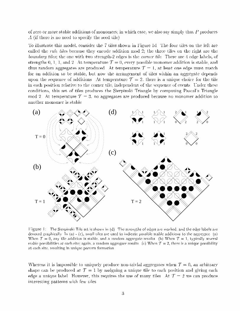
To illustrate this model, consider the 7 tiles shown in Figure 1d. The four tiles on the left are
called the rule tiles because they encode addition mod 2; the three tiles on the right are the
boundary tiles; the one with two strength-2 edges is the corner tile. There are 4 edge labels, of
strengths 0, 1, 1, and 2. At temperature T = 0, every possible monomer addition is stable, and
thus random aggregates are produced. At temperature T = 1, at least one edge must match
for an addition to be stable, but now the arrangement of tiles within an aggregate depends
upon the sequence of additions. At temperature T = 2, there is a unique choice for the tile
in each position relative to the corner tile, independent of the sequence of events. Under these
conditions, this set of tiles produces the Sierpinski Triangle by computing Pascal's Triangle
mod 2. At temperature T = 3, no aggregates are produced because no monomer addition to
another monomer is stable.
(d)
(c)
1
1
1
1 0
2 1
2 0
2
00
2 21
11
1
2
11
1
1
1
1
1 1
1
(a)
T = 0
(b)
T = 2T = 1
Figure 1: The Sierpinski Tile set is shown in (d). The strengths of edges are marked, and the edge labels are
denoted graphically. In (a) - (c), small tiles are used to indicate possible stable additions to the aggregate. (a)
When T = 0, any tile addition is stable, and a random aggregate results. (b) When T = 1, typically several
stable possibilities at each site; again, a random aggregate results. (c) When T = 2, there is a unique possibility
at each site, resulting in unique pattern formation.
Whereas it is impossible to uniquely produce non-trivial aggregates when T = 0, an arbitrary
shape can be produced at T = 1 by assigning a unique tile to each position and giving each
edge a unique label. However, this requires the use of many tiles. At T = 2 we can produce
interesting patterns with few tiles.
3
A hint of the computational power of the Tile Assembly Model when T = 2 is provided by
a simulation of cellular automata2. The proof we develop below demonstrates two important
points. First, even though tile addition is stochastic, a unique pattern is produced regardless
of the order of events, because only stable tile additions are made. Second, the arrangement of
tile types on the 1D growth front of the aggregate can represent information (much like how
the arrangement of 0's and 1's on a 1D tape represents information for a Turing Machine), and
stable tile additions can modify that information by speci�ed rewrite rules, resulting in fully
general computation.
Our simulation is based on one-dimensional blocked cellular automata (BCA)3, a variety of
cellular automaton (CA). It is known that BCA and CA are Turing-universal models, and
simple simulations of Turing machines have been demonstrated (Smith 1971; Biafore preprint).
We begin by de�ning BCA.
De�nition: A k-symbol BCA is de�ned (using the integers f1; 2; : : : ; kg = Zk) by a rule table
R = f(li; ri)! (l0i; r0
i)g � (Zk � Zk ! Zk �Zk):
If R is a function, then the BCA is termed deterministic. The state c of the BCA assigns a
symbol to every location on an in�nite linear array of cells. At each time step every cell in ct is
rewritten to produce ct+1; thus we use ct(x) to denote the symbols written in cell x after t steps.
The BCA uses R to re-write pairs of cells in c, alternating between even and odd alignments
of the pairing: for even t and even x, and for odd t and odd x,
�(ct(x); ct(x + 1))! (ct+1(x); ct+1(x+ 1))
�2 R:
An input to a BCA computation is a state c0 with a �nite number of non-zero cells. For
convenience and without loss of generality, we will con�ne our attention to n-bit binary inputs
b, and write c0 = b to refer to an input where c0(i) = bi for 1 � i � n and c0(i) = 0 otherwise.
The computation of the BCA de�nes ct(x) over the half-plane t � 0. We will show how to
construct a set of tiles P such that in all aggregates produced from the seed tile T0, if there is
a tile at position (i; j) with respect to the seed tile, then the tile has edges encoding ci+j(i� j)
and ci+j(i � j + 1). Thus the time-history of the BCA computation is reproduced exactly in
the self-assembled tile aggregate.
First we show, for any n-bit BCA input b, how to generate the set of n + 3 input tiles I(b).
Figure 2a shows the construction. Because the only edge matches possible with these tiles
are strength 2, at T = 2 all produced aggregates are essentially as shown, with variable length
regions encoding \zero" on either side. The tile whose top edges encode bits b1 and b2 is referred
2This result, presented in less detail in Winfree (1996), translates Wang's simulation of Turing Machine
execution by the Tiling Problem (Wang 1963) into the Tile Assembly Model given here. The Tiling Problem
can be viewed as asking for the ground state of an N-state Ising model, which can be seen as a question of
equilibrium thermodynamics in the limit as T ! 0. Not only can Ising models be produced which are Turing-
universal because the ground state reproduces the space-time history of any chosen Turing Machine, but the
proof that tiles sets can be found which tile the plane non-recursively shows in fact that the ground state of an
Ising model can be non-recursive. Thus it is essential to study a kinetic, rather than thermodynamic, model.3BCA are also known as partitioning CA (Margolus 1984) (a generalization of lattice gas models), as 2-body
CA Biafore (preprint), and by a number of other names.
4
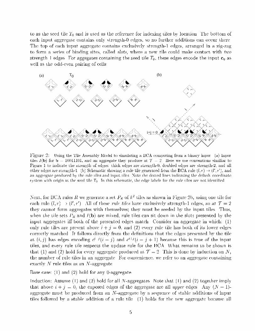
to as the seed tile T0 and is used as the reference for indexing tiles by location. The bottom of
each input aggregate contains only strength-0 edges, so no further additions can occur there.
The top of each input aggregate contains exclusively strength-1 edges, arranged in a zig-zag
to form a series of binding sites, called slots, where a new tile could make contact with two
strength-1 edges. For aggegates containing the seed tile T0, these edges encode the input c0 as
well as the odd-even pairing of cells.
LL s1 s2 s2
s3 s3s4 R R
s4 RL L s1L s2s2 s3 s3 R R
s1LL LL L s2s2 s3 s3 s4 R R R R R
s1 s2LL s2
s3 s3s4 R R R RL
L R Rs1L s2
s2 s3 s3 s4 R R R
s1 s2 s2s3 s3
s4 R R
r’l r
l’
r’l r
l’ r’l r
l’r’l r
l’r’l r
l’
r’l r
l’ r’l r
l’ r’l r
l’
T0 (b)
j
i
i+j = 0
(a)
Figure 2: Using the Tile Assembly Model to simulating a BCA computing from a binary input. (a) Input
tiles I(b) for b = 10011101, and an aggregate they produce at T = 2. Here we use conventions similiar to
Figure 1 to indicate the strength of edges: thick edges are strength-0, doubled edges are strength-2, and all
other edges are strength-1. (b) Schematic showing a rule tile generated from the BCA rule (l; r)! (l0; r0), andan aggregate produced by the rule tiles and input tiles. Note the dotted lines indicating the default coordinate
system with origin at the seed tile T0. In this schematic, the edge labels for the rule tiles are not identi�ed.
Next, for BCA rules R we generate a set PR of k2 tiles as shown in Figure 2b, using one tile for
each rule (l; r) ! (l0; r0). All of these rule tiles have exclusively strength-1 edges, so at T = 2
they cannot form aggregates with themselves; they must be seeded by the input tiles. Thus,
when the tile sets PR and I(b) are mixed, rule tiles can sit down in the slots presented by the
input aggregates i� both of the presented edges match. Consider an aggregate in which: (1)
only rule tiles are present above i + j = 0, and (2) every rule tile has both of its lower edges
correctly matched. It follows directly from the de�nitions that the edges presented by the tile
at (i; j) has edges encoding ci+j(i � j) and c
i+j(i � j + 1) because this is true of the input
tiles, and every rule tile respects the update rule for the BCA. What remains to be shown is
that (1) and (2) hold for every aggregate produced at T = 2. This is done by induction on N ,
the number of rule tiles in an aggregate. For convenience, we refer to an aggregate containing
exactly N rule tiles as an N -aggregate.
Base case: (1) and (2) hold for any 0-aggregate.
Induction: Assume (1) and (2) hold for all N -aggregates. Note that (1) and (2) together imply
that above i + j = 0, the exposed edges of the aggregate are all upper edges. Any (N + 1)-
aggregate must be produced from an N -aggregate by a sequence of stable additions of input
tiles followed by a stable addition of a rule tile. (1) holds for the new aggregate because all
5
exposed edges above i+ j = 0 are upper edges labelled from Zk, while all lower edges of input
tiles are labelled from fL;R; s1; : : : ; sng. (2) holds for the new aggregate because a rule tile
must match two edges to be added, and only upper edges are presented, so the rule tile's two
lower edges must match. 2
Thus, we have proven:
Theorem: Let R be a BCA, and let c(t; x) be the value of cell x at time t for a computation
on input b. If an aggregate produced from seed T0 by the tile set P = PR [ I(b) has a tile in
position (i; j), then the tile's upper edges encode ci+j(i� j) and ci+j(i� j + 1).
In other words, the Tile Assembly Model uses asynchronous and self-timed updates to simulate
any deterministic one-dimensional BCA. Similar arguments can be used to show that the Tile
Assembly Model can simulate any non-deterministic one-dimensional BCA, in the sense that
every possible aggregate produced according to the Tile Assembly Model will represent a pos-
sible history of execution of the non-deterministic BCA. In this case, R will contain rules with
identical left-hand sides, and consequently in some slots multiple rule tiles will match both ex-
posed edges; thus a non-deterministic choice must be made. Alternatively, a non-deterministic
set of input tiles may be used to generate a combinatorial set of possible input strings, followed
by deterministic evaluation of each input. The potential for non-determinism is important for
using self-assembly to solve combinatorial search problems in the spirit of Adleman (1994).
3 Implementation by Self-Assembly of DNA
We followWinfree (1996) in developing a molecular implementation of the Tile Assembly Model:
each tile is represented by a DNA double-crossover (DX) molecule (Fu and Seeman 1993) with
four sticky ends whose sequences represent the edge labels. We would like these molecular
\tiles" to self-assemble into a two-dimensional sheet according to the rules of the Tile Assembly
Model (see Figure 3). Thus, we need to show:
1. Double-crossover molecules can designed to self-assemble into two-dimensional crystal
lattices { in preference over, for example, random tangled nets, tubes, or other structures.
This has in fact now been demonstrated in an experimental system (Winfree et al. 1998).
2. The strengths of edge labels in the model can be implemented by designing the sticky
end sequences with speci�c energetics of hybridization. The DNA hybridization strengths
depend primarly on the number of base pairs, with adjustments for their particular se-
quence, the bu�er conditions, and temperature. Thus, for example, longer sticky ends
can be used to represent edge labels with greater strength.
3. The binding of DX molecules into slots, where two sticky end sequences must both hy-
bridize, is cooperative { thus, strengths \add". We will argue below that this is a priori
likely; furthermore, suggestive experimental evidence has been presented in Winfree et al.
(in press).
6
4. There is a physical parameter analogous to T which determines the strength required
for association of molecular tiles. This parameter can be, for example, the temperature
T . DNA sticky ends bind more strongly at low temperatures, and conversely, at higher
temperatures more sticky-end interactions will be necessary for stable addition.
5. All these considerations can come together to produce molecular self-assembly in accor-
dance with the Tile Assembly Model.
r’l r
l’
W(l)
C(l’) C(r’)
W(r)
(a) (b)
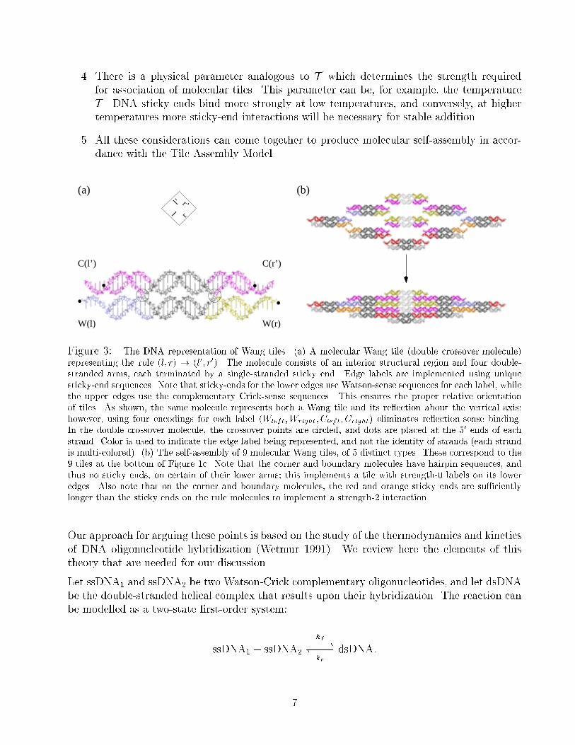
Figure 3: The DNA representation of Wang tiles. (a) A molecular Wang tile (double crossover molecule)
representing the rule (l; r) ! (l0; r0). The molecule consists of an interior structural region and four double-
stranded arms, each terminated by a single-stranded sticky end. Edge labels are implemented using unique
sticky-end sequences. Note that sticky-ends for the lower edges use Watson-sense sequences for each label, while
the upper edges use the complementary Crick-sense sequences. This ensures the proper relative orientation
of tiles. As shown, the same molecule represents both a Wang tile and its re ection about the vertical axis;
however, using four encodings for each label (Wleft;Wright; Cleft; Cright) eliminates re ection-sense binding.
In the double crossover molecule, the crossover points are circled, and dots are placed at the 50 ends of eachstrand. Color is used to indicate the edge label being represented, and not the identity of strands (each strand
is multi-colored). (b) The self-assembly of 9 molecular Wang tiles, of 5 distinct types. These correspond to the
9 tiles at the bottom of Figure 1c. Note that the corner and boundary molecules have hairpin sequences, and
thus no sticky ends, on certain of their lower arms; this implements a tile with strength-0 labels on its lower
edges. Also note that on the corner and boundary molecules, the red and orange sticky ends are su�ciently
longer than the sticky ends on the rule molecules to implement a strength-2 interaction.
Our approach for arguing these points is based on the study of the thermodynamics and kinetics
of DNA oligonucleotide hybridization (Wetmur 1991). We review here the elements of this
theory that are needed for our discussion.
Let ssDNA1 and ssDNA2 be two Watson-Crick complementary oligonucleotides, and let dsDNA
be the double-stranded helical complex that results upon their hybridization. The reaction can
be modelled as a two-state �rst-order system:
ssDNA1 + ssDNA2
kf���*)���kr
dsDNA:
7
We can write a di�erential equation for the rates of change of the concentration of each species.
The units for kr are 1/sec, so kr [dsDNA] gives the rate in M/sec of dissociation of the dou-
ble helix; the units for kf are 1/M/sec, so kf [ssDNA1][ssDNA2] gives the rate in M/sec of
hybridization to form new double helical molecules. Altogether, we have:
� _[dsDNA] = _[ssDNA1] =_[ssDNA2] = kr [dsDNA]� kf [ssDNA1][ssDNA2]
The rate constants kf and kr can be estimated from the DNA sequence and the temperature
T (in K), assuming the reaction is taking place in a standard bu�er. For very short oligonu-
cleotides, the forward reaction has a di�usion-controlled rate-determining step (Quartin and
Wetmur 1989) approximately independent of oligo length and sequence, so:
kf = Af e�Ef=RT � 6� 105 /M/sec;
where Af = 5�108 /M/sec and Ef = 4kcal/mol is the activation energy for the reaction4. The
reverse rate, on the other hand, is very sensitive to oligo length and sequence:
kr = kfe�G�
s=RT ;
where R = 2 cal/mol/K and �G�
s < 0 is the free energy released as heat by a single hybridization
event5. The standard free energy �G�
s can be calculated from the standard enthalpy �H�
s and
the standard entropy �S�
s of the reaction: �G�
s = �H�
s � T�S�
s . For reactions taking place
in commonly used bu�ers, the standard enthalpy and entropy can be reliably estimated from
the sequence according to a nearest-neighbor model (SantaLucia et al. 1996); however, for the
purposes of this discussion, we can use the coarser approximation for length-s oligonucleotides6:
�H�
s � �8s kcal/mol and �S�
s � �22s� 6 cal/mol/K. Thus we can predict both kf and kr for
the hybridization of complementary oligonucleotides. This allows us to predict the equilibrium
concentrations of each species via the equilibrium constant
K:=
[dsDNA]
[ssDNA1][ssDNA2]=kf
kr= e
��G�
s=RT :
We will use our understanding of oligonucleotide hybridization kinetics and thermodynamics
to build a plausible model for the self-assembly of DX molecules via the hybridization of their
sticky ends.
4We will ignore the activation energy in what follows, because we will see that the value of kf has no e�ect
on the behavior of the system except to set the scale of the time axis.5The more negative �G�
s is, the more heat is released upon association and the more favorable the reaction
is. Another way of looking at it is that if �G�s is very negative, a lot of heat must simultaneously converge
upon a single double helical DNA molecule in order to cause dissociation, and thus dissociation is rare. Also
note that here, as elsewhere, e�G�
s=RT has an \invisible" unit of M, so that kr is in units of 1/sec.
6The empirical value �Sinit = �6 cal/mol/K can be considered the entropic cost of aligning the two strands
to have the same orientation, and is called the initiation entropy.
8
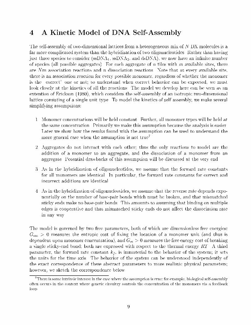
4 A Kinetic Model of DNA Self-Assembly
The self-assembly of two-dimensional lattices from a heterogeneous mix of N DX molecules is a
far more complicated system than the hybridization of two oligonucleotides. Rather than having
just three species to consider (ssDNA1, ssDNA2, and dsDNA), we now have an in�nite number
of species (all possible aggregates). For each aggregate of n tiles with m available sites, there
are Nm association reactions and n dissociation reactions. Note that at every available site,
there is an association reaction for every possible monomer, regardless of whether the monomer
is the \correct" one or not; to understand when correct behavior can be expected, we must
look closely at the kinetics of all the reactions. The model we develop here can be seen as an
extention of Erickson (1980), which considers the self-assembly of an isotropic two-dimensional
lattice consisting of a single unit type. To model the kinetics of self-assembly, we make several
simplifying assumptions:
1. Monomer concentrations will be held constant. Further, all monomer types will be held at
the same concentration. Primarily we make this assumption because the analysis is easier.
Later we show how the results found with the assumption can be used to understand the
more general case when the assumption is not true7.
2. Aggregates do not interact with each other; thus the only reactions to model are the
addition of a monomer to an aggregate, and the dissociation of a monomer from an
aggregate. Potential drawbacks of this assumption will be discussed at the very end.
3. As in the hybridization of oligonucleotides, we assume that the forward rate constants
for all monomers are identical. In particular, the forward rate constants for correct and
incorrect additions are identical.
4. As in the hybridization of oligonucleotides, we assume that the reverse rate depends expo-
nentially on the number of base-pair bonds which must be broken, and that mismatched
sticky ends make no base-pair bonds. This amounts to assuming that binding on multiple
edges is cooperative and that mismatched sticky ends do not a�ect the dissociation rate
in any way.
The model is governed by two free parameters, both of which are dimensionless free energies:
Gmc > 0 measures the entropic cost of �xing the location of a monomer unit (and thus is
dependent upon monomer concentration), andGse > 0 measures the free energy cost of breaking
a single sticky-end bond; both are expressed with respect to the thermal energy RT . A third
parameter, the forward rate constant kf , is immaterial to the behavior of the system; it sets
the units for the time axis. The behavior of the system can be understood independently of
the exact correspondence of these abstract parameters to more realistic physical parameters;
however, we sketch the correspondence below.
7There is some intrinsic interest in the case where the assumption is true; for example, biological self-assembly
often occurs in the context where genetic circuitry controls the concentration of the monomers via a feedback
loop.
9
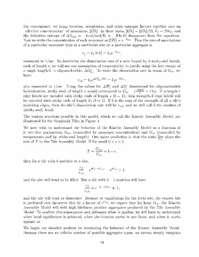
For convenience, we lump location, orientation, and other entropic factors together into an
\e�ective concentration" of monomers, [D̂X]. In these units, [D̂X] = [DX]=20, k̂f = 20kf , and
the initiation entropy of �Sinit = �6 cal/mol/K = �R ln 20 disappears from the equations.
Now we write the concentration of each monomer as [D̂X] = e�Gmc. Thus the rate of associations
of a particular monomer type at a particular site on a particular aggregate is
rf = kf [DX] = k̂fe�Gmc ;
measured in 1/sec. To determine the dissociation rate of a unit bound by b sticky-end bonds,
each of length s, we will use our assumption of cooperativity to justify using the free energy of
a single length-b � s oligonucleotide, �G�
b�s. To write the dissociation rate in terms of Gse, we
have:
rr;b = kfe�G�
b�s=RT = k̂fe
�bGse ;
also measured in 1/sec. Using the values for �H�
s and �S�
s determined for oligonucleotide
hybridization, sticky ends of length s would correspond to Gse = (4000KT
� 11)s. If strength-1
edge labels are encoded with sticky ends of length s (b = 1), then strength-2 edge labels will
be encoded with sticky ends of length 2s (b = 2). If b is the sum of the strength of all a tile's
matching edges, then the tile's dissociation rate will be rr;b, and we will call b the number of
(sticky-end) bonds.
The various reactions possible in this model, which we call the Kinetic Assembly Model, are
illustrated for the Sierpinski Tiles in Figure 4.
We now wish to understand the behavior of the Kinetic Assembly Model as a function of
it two free parameters, Gmc (controlled by monomer concentration) and Gse (controlled by
temperature and by sticky-end length). Our naive prediction is that the ratio Gmc
Gseplays the
role of T in the Tile Assembly Model. If for small 0 < � < 1
T :=Gmc
Gse
= b� �;
then for a tile with b matches at a site,
rf
rr;b= e
bGse�Gmc = e�Gse > 1;
and the site will tend to be �lled. But a tile with b� 1 matches will have
rf
rr;b= e
�(1��)Gse � 1;
and the tile will tend to dissociate. Because at equilibrium for the local site, the correct tile
is preferred over incorrect tiles by a factor of eGse , we expect that for large Gse, the Kinetic
Assembly Model will with high likeliness produce aggregates produced by the Tile Assembly
Model. To con�rm this expectation and delineate when it applies, we will have to understand
when local equilibrium is achieved, when the kinetics works in our favor, and when it works
against us.
We begin our detailed analysis by simulating the behavior of the Kinetic Assembly Model.
Because there are an in�nite number of possible aggregate types, we cannot simply integrate
10
rf
rr,0
rf rr,2rf rr,1
rf
rr,1 rf
rr,2
rf
rr,5
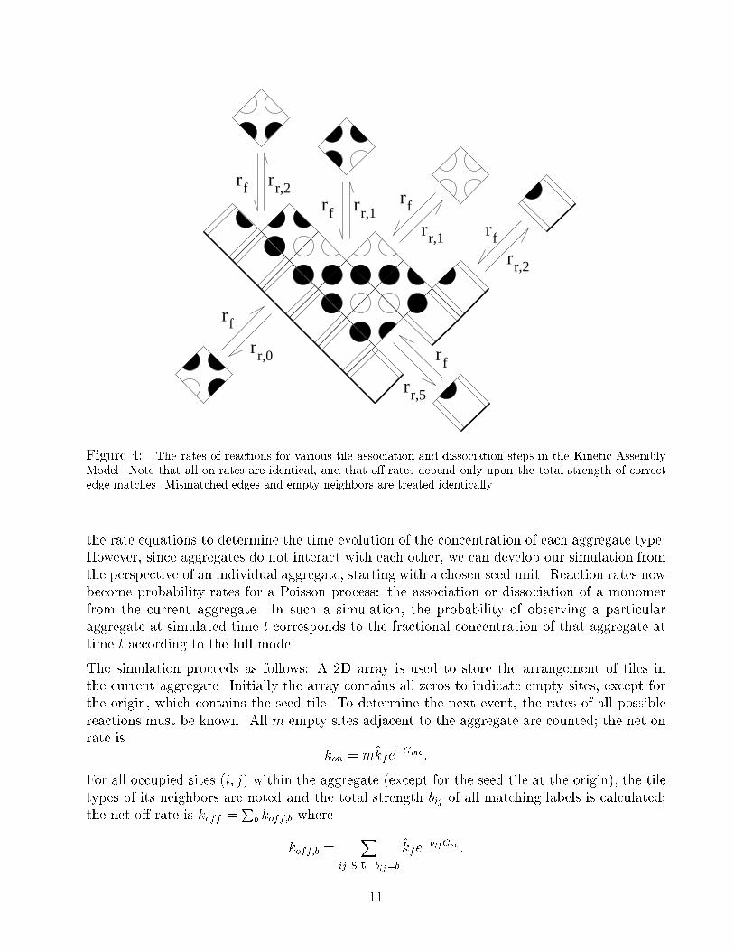
Figure 4: The rates of reactions for various tile association and dissociation steps in the Kinetic Assembly
Model. Note that all on-rates are identical, and that o�-rates depend only upon the total strength of correct
edge matches. Mismatched edges and empty neighbors are treated identically.
the rate equations to determine the time evolution of the concentration of each aggregate type.
However, since aggregates do not interact with each other, we can develop our simulation from
the perspective of an individual aggregate, starting with a chosen seed unit. Reaction rates now
become probability rates for a Poisson process: the association or dissociation of a monomer
from the current aggregate. In such a simulation, the probability of observing a particular
aggregate at simulated time t corresponds to the fractional concentration of that aggregate at
time t according to the full model.
The simulation proceeds as follows: A 2D array is used to store the arrangement of tiles in
the current aggregate. Initially the array contains all zeros to indicate empty sites, except for
the origin, which contains the seed tile. To determine the next event, the rates of all possible
reactions must be known. All m empty sites adjacent to the aggregate are counted; the net on
rate is
kon = mk̂fe�Gmc :
For all occupied sites (i; j) within the aggregate (except for the seed tile at the origin), the tile
types of its neighbors are noted and the total strength bij of all matching labels is calculated;
the net o� rate is koff =P
b koff;b where
koff;b =X
ij s.t. bij=b
k̂fe�bijGse:
11
Thus the net rate for events of any kind is kany = kon + koff , and the time until the next event
occurs, �t, is chosen according to the Boltzman distribution Pr(�t) = kanyekany�t. Now, given
that an event has occurred, the probability that it is an on-event is kon=kany, in which case all
sites and all tile types are equally likely to be chosen; otherwise a dissociation has occurred,
and the probability that some site with b bonds dissociates is koff;b=koff , and again all such
sites are equally likely. Once the event is chosen and the array is updated, all rates must be
recalculated to determine the next event8.
5 Simulation Results
This section discusses simulations of the self-assembly of the Sierpinski Tiles using the Kinetic
Assembly Model. An example run is shown in Figure 5. Several features of this simulation run
warrant comment.
Shape: The growth front does not advance synchronously, but rather performs a biased random
walk, with the following restriction: because stable addition occurs only at concave corner
sites (slots) on the growth front, no sites can be more than one step ahead of or behind
its neighbors. The growth front is concave on average: the boundary tiles grow fastest
because their growth site is always available, while internal regions on the growth front
grow slower because stable addition can occur at only a fraction of sites at any given time.
Errors: For the most part, the Sierpinski Triangle is accurately reproduced. However, incorrect
tiles do appear. In the �rst three frames, incorrect tiles can be seen on the border of the
aggregate. These are inconsequential errors due to the equal on-rates of all tiles; they will
fall o� immediately and cause no permanent errors. However, in the last frame we see an
incorrect tile which has been embedded within the aggregate; although it has a mismatch
with its predecessors, successive tile additions have been correct with respect to the error,
and now the erroneous tile has 3 matched edges. It has caused a permanent error, and
the misinformation spreads to all downstream cells in the computation.
Array Size: In the last two frames, the size of the aggregate has exceeded the size of the array
used in the simulation. Thus the Kinetic Assembly Model is not perfectly simulated; a
maximal size of aggregate is imposed. In the simulations below, this does not a�ect the
results in the region of interest, but it does explain the constant size (the maximum)
found during fast, random aggregation.
To map out the parameter space of this model, simulations of the Sierpinski tiles were performed
for all 1 � Gmc; Gse � 30. Each simulation was run for 60=rf simulated seconds, thus on
average each unoccupied site could experience up to 60 on-events of each type; consequently,
the distribution of aggregate sizes is comparable across di�erent parameter values. Figure 6
shows the results for (a) aggregates seeded by the corner tile and (b) aggregates seeded by a
8The actual computer code is optimized to remove redundant calculations, of course!
12
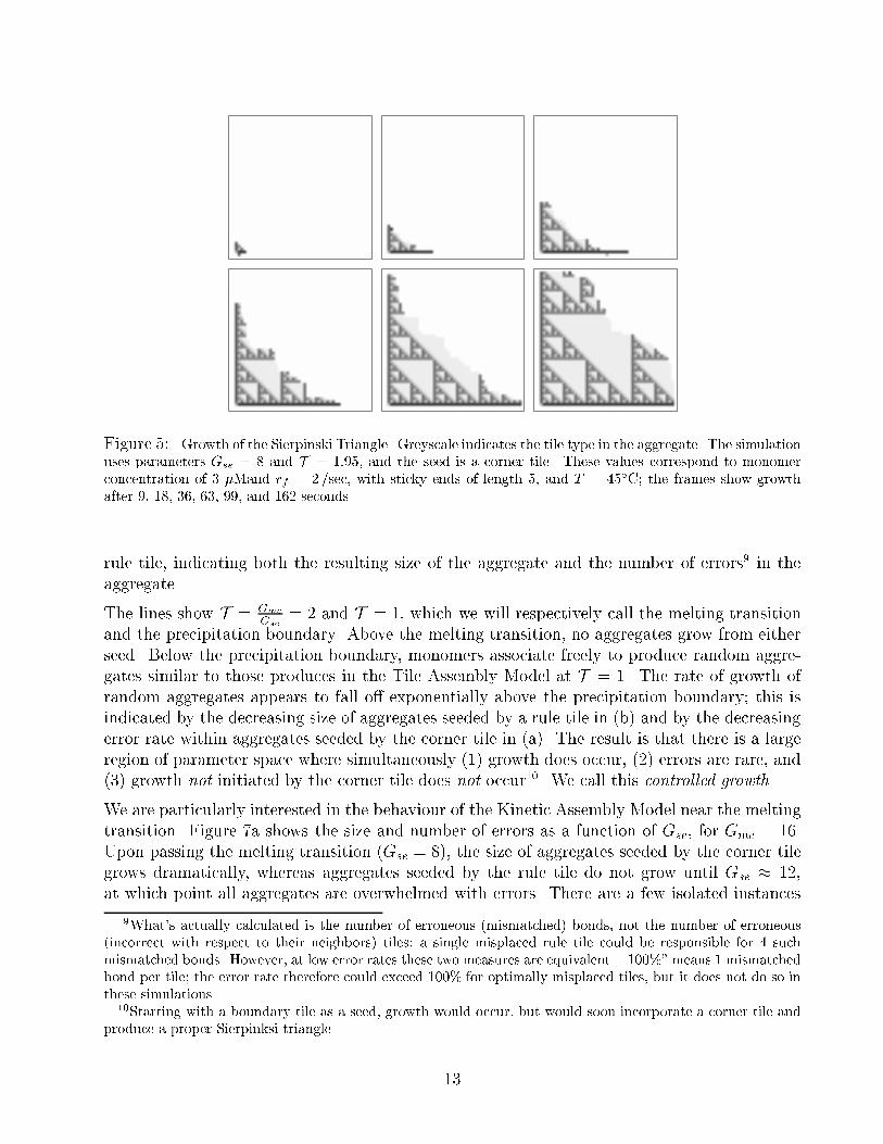
Figure 5: Growth of the Sierpinski Triangle. Greyscale indicates the tile type in the aggregate. The simulation
uses parameters Gse = 8 and T = 1:95, and the seed is a corner tile. These values correspond to monomer
concentration of 3 �Mand rf = 2/sec, with sticky ends of length 5, and T = 45�C; the frames show growth
after 9, 18, 36, 63, 99, and 162 seconds.
rule tile, indicating both the resulting size of the aggregate and the number of errors9 in the
aggregate.
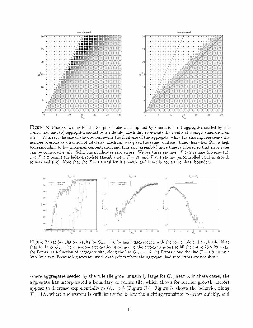
The lines show T = Gmc
Gse= 2 and T = 1, which we will respectively call the melting transition
and the precipitation boundary. Above the melting transition, no aggregates grow from either
seed. Below the precipitation boundary, monomers associate freely to produce random aggre-
gates similar to those produces in the Tile Assembly Model at T = 1. The rate of growth of
random aggregates appears to fall o� exponentially above the precipitation boundary; this is
indicated by the decreasing size of aggregates seeded by a rule tile in (b) and by the decreasing
error rate within aggregates seeded by the corner tile in (a). The result is that there is a large
region of parameter space where simultaneously (1) growth does occur, (2) errors are rare, and
(3) growth not initiated by the corner tile does not occur10. We call this controlled growth.
We are particularly interested in the behaviour of the Kinetic Assembly Model near the melting
transition. Figure 7a shows the size and number of errors as a function of Gse, for Gmc = 16.
Upon passing the melting transition (Gse = 8), the size of aggregates seeded by the corner tile
grows dramatically, whereas aggregates seeded by the rule tile do not grow until Gse � 12,
at which point all aggregates are overwhelmed with errors. There are a few isolated instances
9What's actually calculated is the number of erroneous (mismatched) bonds, not the number of erroneous
(incorrect with respect to their neighbors) tiles; a single misplaced rule tile could be responsible for 4 such
mismatched bonds. However, at low error rates these two measures are equivalent. \100%" means 1 mismatched
bond per tile; the error rate therefore could exceed 100% for optimally misplaced tiles, but it does not do so in
these simulations.10Starting with a boundary tile as a seed, growth would occur, but would soon incorporate a corner tile and
produce a proper Sierpinksi triangle.
13
0 5 10 15 20 25 300
5
10
15
20
25
30
Gse
Gm
c
corner tile seed
0 5 10 15 20 25 300
5
10
15
20
25
30
Gse
Gm
c
rule tile seed
Figure 6: Phase diagrams for the Sierpinski tiles as computed by simulation: (a) aggregates seeded by the
corner tile, and (b) aggregates seeded by a rule tile. Each disc represents the results of a single simulation on
a 28� 28 array; the size of the disc represents the �nal size of the aggregate, while the shading represents the
number of errors as a fraction of total size. Each run was given the same \unitless" time; thus when Gmc is high
(corresponding to low monomer concentration and thus slow assembly) more time is allowed so that error rates
can be compared easily. Solid black indicates zero errors. We see three regimes: T > 2 regime (no growth),
1 < T < 2 regime (includes error-free assembly near T = 2), and T < 1 regime (uncontrolled random growth
to maximal size). Note that the T = 1 transition is smooth, and hence is not a true phase boundary.
7 8 9 10 11 12 13 14 15 160
100
200
300
400
500
600
700
800
Gse
size
Gmc
= 16
corner seedrule seed
7 8 9 10 11 12 13 14 15 16
10−3
10−2
10−1
100
Gse
erro
r fr
actio
n
Gmc
= 16
corner seedrule seed
0 2 4 6 8 10 12 14 16
10−3
10−2
10−1
100
Gse
Gmc
= 1.9 Gse
erro
r fr
actio
n
corner seed
Figure 7: (a) Simulation results for Gmc = 16 for aggregates seeded with the corner tile and a rule tile. Note
that for large Gse, where random aggregation is occurring, the aggregate grows to �ll the entire 28� 28 array.
(b) Errors, as a fraction of aggregate size, along the line Gmc = 16. (c) Errors along the line T = 1:9, using a
38� 38 array. Because log axes are used, data points where the aggregate had zero errors are not shown.
where aggregates seeded by the rule tile grow unusually large for Gse near 8; in these cases, the
aggregate has incorporated a boundary or corner tile, which allows for further growth. Errors
appear to decrease exponentially as Gse ! 8 (Figure 7b). Figure 7c shows the behavior along
T = 1:9, where the system is su�ciently far below the melting transition to grow quickly, and
14
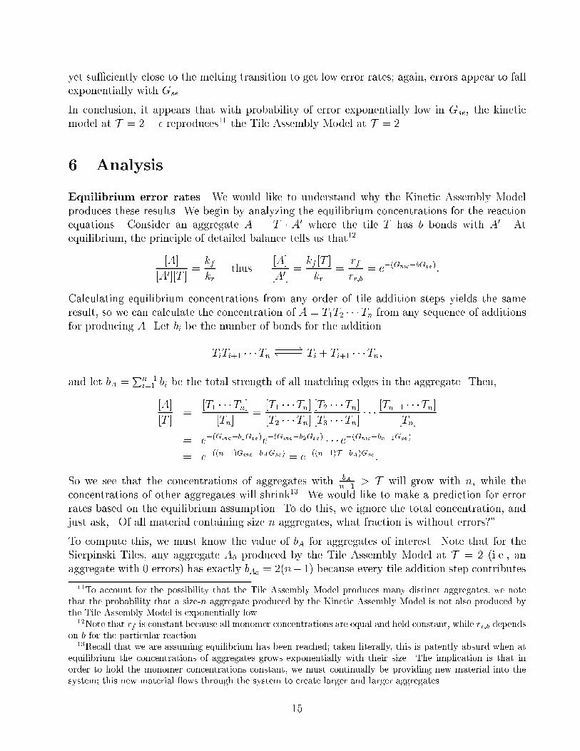
yet su�ciently close to the melting transition to get low error rates; again, errors appear to fall
exponentially with Gse.
In conclusion, it appears that with probability of error exponentially low in Gse, the kinetic
model at T = 2� � reproduces11 the Tile Assembly Model at T = 2.
6 Analysis
Equilibrium error rates. We would like to understand why the Kinetic Assembly Model
produces these results. We begin by analyzing the equilibrium concentrations for the reaction
equations. Consider an aggregate A = T � A0 where the tile T has b bonds with A0. At
equilibrium, the principle of detailed balance tells us that12
[A]
[A0][T ]=kf
krthus
[A]
[A0]=kf [T ]
kr=
rf
rr;b= e
�(Gmc�bGse):
Calculating equilibrium concentrations from any order of tile addition steps yields the same
result, so we can calculate the concentration of A = T1T2 � � �Tn from any sequence of additions
for producing A. Let bi be the number of bonds for the addition
TiTi+1 � � �Tn ���*)��� Ti + Ti+1 � � �Tn;
and let bA =Pn�1
i=1 bi be the total strength of all matching edges in the aggregate. Then,
[A]
[T ]=
[T1 � � �Tn][Tn]
=[T1 � � �Tn][T2 � � �Tn]
[T2 � � �Tn][T3 � � �Tn]
� � � [Tn�1 � � �Tn][Tn]
= e�(Gmc�b1Gse)e
�(Gmc�b2Gse) � � � e�(Gmc�bn�1Gse)
= e�((n�1)Gmc�bAGse) = e
�((n�1)T �bA)Gse :
So we see that the concentrations of aggregates with bAn�1
> T will grow with n, while the
concentrations of other aggregates will shrink13. We would like to make a prediction for error
rates based on the equilibrium assumption. To do this, we ignore the total concentration, and
just ask, \Of all material containing size n aggregates, what fraction is without errors?"
To compute this, we must know the value of bA for aggregates of interest. Note that for the
Sierpinski Tiles, any aggregate A0 produced by the Tile Assembly Model at T = 2 (i.e., an
aggregate with 0 errors) has exactly bA0= 2(n� 1) because every tile addition step contributes
11To account for the possibility that the Tile Assembly Model produces many distinct aggregates, we note
that the probability that a size-n aggregate produced by the Kinetic Assembly Model is not also produced by
the Tile Assembly Model is exponentially low.12Note that rf is constant because all monomer concentrations are equal and held constant, while rr;b depends
on b for the particular reaction.13Recall that we are assuming equilibrium has been reached; taken literally, this is patently absurd when at
equilibrium the concentrations of aggregates grows exponentially with their size. The implication is that in
order to hold the monomer concentrations constant, we must continually be providing new material into the
system; this new material ows through the system to create larger and larger aggregates.
15
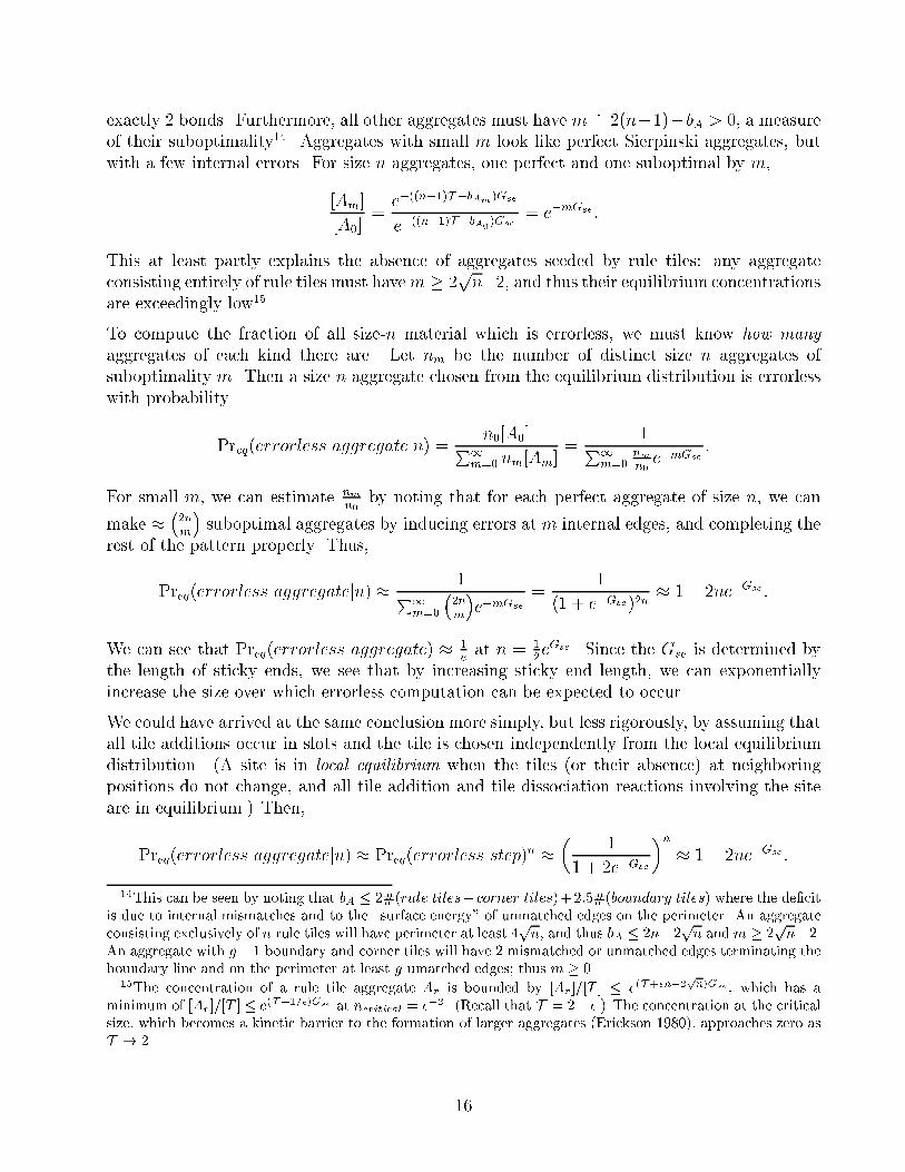
exactly 2 bonds. Furthermore, all other aggregates must have m:= 2(n�1)�bA > 0, a measure
of their suboptimality14. Aggregates with small m look like perfect Sierpinski aggregates, but
with a few internal errors. For size n aggregates, one perfect and one suboptimal by m,
[Am]
[A0]=e�((n�1)T �bAm )Gse
e�((n�1)T �bA0
)Gse= e
�mGse :
This at least partly explains the absence of aggregates seeded by rule tiles: any aggregate
consisting entirely of rule tiles must havem � 2pn�2, and thus their equilibrium concentrations
are exceedingly low15.
To compute the fraction of all size-n material which is errorless, we must know how many
aggregates of each kind there are. Let nm be the number of distinct size n aggregates of
suboptimality m. Then a size n aggregate chosen from the equilibrium distribution is errorless
with probability
Preq(errorless aggregatejn) = n0[A0]P1
m=0 nm[Am]=
1P1
m=0nmn0e�mGse
:
For small m, we can estimate nmn0
by noting that for each perfect aggregate of size n, we can
make ��2n
m
�suboptimal aggregates by inducing errors at m internal edges, and completing the
rest of the pattern properly. Thus,
Preq(errorless aggregatejn) � 1P1
m=0
�2n
m
�e�mGse
=1
(1 + e�Gse)2n� 1� 2ne�Gse :
We can see that Preq(errorless aggregate) � 1eat n = 1
2eGse . Since the Gse is determined by
the length of sticky ends, we see that by increasing sticky end length, we can exponentially
increase the size over which errorless computation can be expected to occur.
We could have arrived at the same conclusion more simply, but less rigorously, by assuming that
all tile additions occur in slots and the tile is chosen independently from the local equilibrium
distribution. (A site is in local equilibrium when the tiles (or their absence) at neighboring
positions do not change, and all tile addition and tile dissociation reactions involving the site
are in equilibrium.) Then,
Preq(errorless aggregatejn) � Preq(errorless step)n �
�1
1 + 2e�Gse
�n� 1� 2ne�Gse :
14This can be seen by noting that bA � 2#(rule tiles+ corner tiles)+2:5#(boundary tiles) where the de�cit
is due to internal mismatches and to the \surface energy" of unmatched edges on the perimeter. An aggregate
consisting exclusively of n rule tiles will have perimeter at least 4pn, and thus bA � 2n�2pn and m � 2
pn�2.
An aggregate with g+1 boundary and corner tiles will have 2 mismatched or unmatched edges terminating the
boundary line and on the perimeter at least g umatched edges; thus m � 0.15The concentration of a rule tile aggregate Ar is bounded by [Ar ]=[T ] � e(T+�n�2
pn)Gse , which has a
minimum of [Ar]=[T ] � e(T �1=�)Gse at ncritical = ��2. (Recall that T = 2� �.) The concentration at the critical
size, which becomes a kinetic barrier to the formation of larger aggregates (Erickson 1980), approaches zero as
T ! 2.
16
Note that this analysis, based on assumptions of equilibrium, predicts that error rates are
una�ected by Gmc. This was not the result of our simulation: error rates increase dramat-
ically as Gmc drops below the melting transition (i.e., as monomer concentration increases).
Consequently, we conclude that equilibrium is not achieved in these cases.
The kinetic trap. What prevents the system from achieving equilibrium? The intuition is
that if the growth of the crystal is faster than the time required to locally establish equilibrium
at the growth sites, tiles will become embedded and \frozen" in the interior of the aggregate
with an out-of-equilibrium distribution.
How long does it take for a growth site to reach local equilibrium? Consider a growth site
that has just formed, and assume that the local context (neighboring tiles) does not change.
Monomer tiles of all kinds will sit down at the site, stay a while, and then leave, each according
to its own o�-rate. If we look immediately after the growth site appears, the probability that
the site is empty is near 100%; however, if we wait a very long time before looking, we will
�nd each tile, or an empty site, with their equilibrium probabilities. If the local context does
change by addition of tiles surrounding the growth site, then the tile currently in place can be
\frozen" there e�ectively permanently; even if it has one mismatched edge, three matches on
its other edges can make its o�-rate very low. Although this is a very cartoonish picture, it is
the basis for our analysis, since the full system is too complex to treat rigorously.
rr,1
rr,0
rf rr,2
r*
r*
r*
E Af
I FI
4rf
2r
C FC
0 2 4 6 8
x 10−4
0
0.1
0.2
0.3
0.4
0.5
0.6
0.7
0.8
0.9
1
seconds
prob
abili
ty
Approach to equilibrium (Gse
=3, Gmc
=5)
Empty siteCorrect tileIncorrect tiles
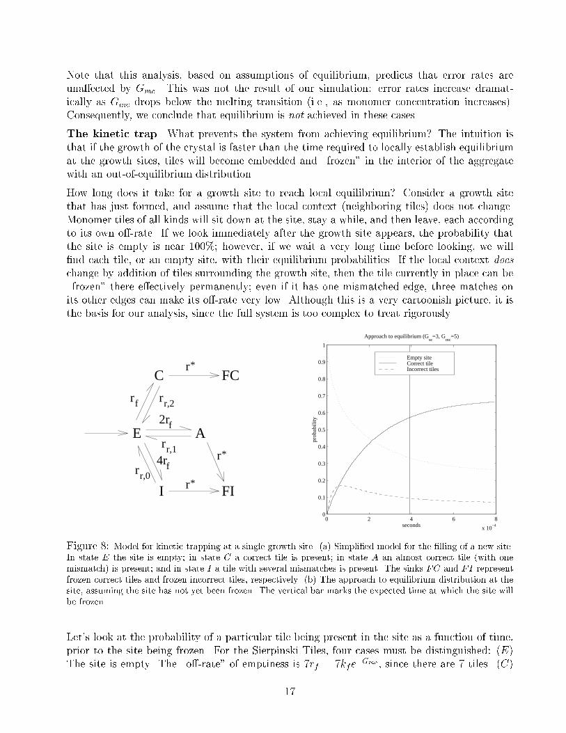
Figure 8: Model for kinetic trapping at a single growth site. (a) Simpli�ed model for the �lling of a new site.
In state E the site is empty; in state C a correct tile is present; in state A an almost correct tile (with one
mismatch) is present; and in state I a tile with several mismatches is present. The sinks FC and FI represent
frozen correct tiles and frozen incorrect tiles, respectively. (b) The approach to equilibrium distribution at the
site, assuming the site has not yet been frozen. The vertical bar marks the expected time at which the site will
be frozen.
Let's look at the probability of a particular tile being present in the site as a function of time,
prior to the site being frozen. For the Sierpinski Tiles, four cases must be distinguished: (E)
The site is empty. The \o�-rate" of emptiness is 7rf = 7kfe�Gmc , since there are 7 tiles. (C)
17
The correct tile is in place. It's o�-rate is rr;2 = kfe�2Gse . (A) One of two tiles with just one
match, and o�-rate rr;1 = kfe�Gse . (I) One of 4 tiles with no matches, and o�-rate rr;0 = kf .
Let pi(t) be the probability that (i) is the case t seconds after the growth site has appeared,
assuming the site has not yet been frozen. The rate equations for the model in Figure 8a,
excluding the sinks FC and FI, can be written as
_p(t) =
26664�7rf rr;2 rr;1 rr;0
rf �rr;2 0 0
2rf 0 �rr;1 0
4rf 0 0 �rr;0
37775
26664pE(t)
pC(t)
pA(t)
pI(t)
37775:=Mp(t)
and thus, p(t) = eMtp(0) where p(0) = [1 0 0 0]T .
The behavior of p(t) is shown in Figure 8b. We want to know the probability that the correct tile
is in place when the site is frozen. During controlled growth, the rate of growth is approximately
r� = rf � rr;2; thus a given site will be frozen in mean time approximately t� = 1=(rf � rr;2).
With a decrease inGmc (increased monomer concentration), rf increases, and t� becomes earlier,
leading to a more out-of-equilibrium frozen distribution.
By including sink states FC and FI into the model of Figure 8a, we can solve exactly for the
frozen distribution. In this case the equations are
_p(t) =
2666666664
�7rf rr;2 rr;1 rr;0 0 0
rf �rr;2 � r� 0 0 0 0
2rf 0 �rr;1 � r� 0 0 0
4rf 0 0 �rr;0 � r� 0 0
0 r� 0 0 0 0
0 0 r�
r� 0 0
3777777775
2666666664
pE(t)
pC(t)
pA(t)
pI(t)
pFC(t)
pFI(t)
3777777775:=Mp(t)
where p(0) = [1 0 0 0 0 0]T . The probability of the site being frozen with the correct tile,
pFC(1), can be easily computed from the steady-state of the related ow problem, where a
unit amount of material is pumped into state E and accumulates di�erentially in FC and FI:
_p(1) = [1 0 0 0 pFC(1) pFI(1)]T =Mp(1):
A little algebra gives the probability of an errorless step in terms of Gse and Gmc:
Prkin(errorless step):= pFC(1) =
1r�+rr;2
1r�+rr;2
+ 2r�+rr;1
+ 4r�+rr;0
:
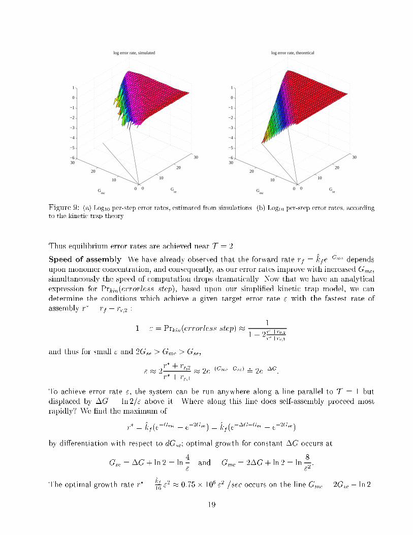
In this equation for errors due to kinetic trapping, in contrast to the equilibrium prediction,
the error rate depends upon both Gse and Gmc. The equation predicts error rates that are in
qualitative agreement with the simulations, as shown in Figure 9. In this analysis, it becomes
clear that in the limit as T ! 2 and thus r� ! 0,
Prkin(errorless step)! Preq(errorless step) =1=rr;2
1=rr;2 + 2=rr;1 + 4=rr;0� 1
1 + 2e�Gse:
18
0
10
20
30
0
10
20
30−6
−5
−4
−3
−2
−1
0
1
Gse
log error rate, simulated
Gmc
0
10
20
30
0
10
20
30−6
−5
−4
−3
−2
−1
0
1
Gse
log error rate, theoretical
Gmc
Figure 9: (a) Log10 per-step error rates, estimated from simulations. (b) Log10 per-step error rates, according
to the kinetic trap theory.
Thus equilibrium error rates are achieved near T = 2.
Speed of assembly. We have already observed that the forward rate rf = k̂fe�Gmc depends
upon monomer concentration, and consequently, as our error rates improve with increased Gmc,
simultaneously the speed of computation drops dramatically. Now that we have an analytical
expression for Prkin(errorless step), based upon our simpli�ed kinetic trap model, we can
determine the conditions which achieve a given target error rate " with the fastest rate of
assembly r� = rf � rr;2 :
1� " = Prkin(errorless step) � 1
1 + 2r�+rr;2r�+rr;1
and thus for small " and 2Gse > Gmc > Gse,
" � 2r� + rr;2
r� + rr;1� 2e�(Gmc�Gse) :
= 2e��G:
To achieve error rate ", the system can be run anywhere along a line parallel to T = 1 but
displaced by �G = ln 2=" above it. Where along this line does self-assembly proceed most
rapidly? We �nd the maximum of
r� = k̂f(e
�Gmc � e�2Gse) = k̂f(e
��G�Gse � e�2Gse)
by di�erentiation with respect to dGse; optimal growth for constant �G occurs at
Gse = �G+ ln 2 = ln4
"and Gmc = 2�G+ ln 2 = ln
8
"2:
The optimal growth rate r� =k̂f16"2 � 0:75� 106 "2 =sec occurs on the line Gmc = 2Gse � ln 2.
19
T = 1
constant εgrowthoptimal
T = 2free
monomer
aggregationrandom
Gse
Gmc
∆ G
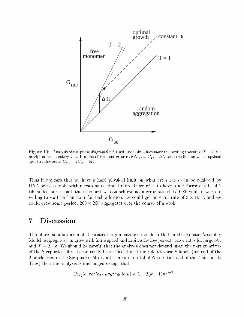
Figure 10: Analysis of the phase diagram for 2D self-assembly. Lines mark the melting transition T = 2, the
precipitation boundary T = 1, a line of constant error rate Gmc = Gse +�G, and the line on which optimal
growth rates occur Gmc = 2Gse � ln 2.
Thus it appears that we have a hard physical limit on what error rates can be achieved by
DNA self-assembly within reasonable time limits. If we wish to have a net forward rate of 1
tile added per second, then the best we can achieve is an error rate of 1/1000; while if we were
willing to wait half an hour for each addition, we could get an error rate of 3 � 10�5, and we
could grow some perfect 200� 200 aggregates over the course of a week.
7 Discussion
The above simulations and theoretical arguments both con�rm that in the Kinetic Assembly
Model, aggregates can grow with �nite speed and arbitrarily low per-site error rates for largeGse
and T = 2� �. We should be careful that the analysis does not depend upon the particularities
of the Sierpinski Tiles. It can easily be veri�ed that if the rule tiles use k labels (instead of the
2 labels used in the Sierpinski Tiles) and there are a total of N tiles (instead of the 7 Sierpinski
Tiles) then the analysis is unchanged except that
Preq(errorless aggregatejn) � 1� 2(k � 1)ne�Gse
20
and
Prkin(errorless step) =
1r�+rr;2
1r�+rr;2
+2(k�1)
r�+rr;1+
N�1�2(k�1)
r�+rr;0
� 1� 2(k � 1)e�(Gmc�Gse)
and the optimal growth rate now occurs displaced �G =ln 2(k�1)
"above T = 1. We now loosely
discuss other aspects of the model.
Energy use. Reversible computers have the potential to compute using arbitrarily little en-
ergy per step, because no information is erased during the computation itself (Landauer 1961;
Bennett 1973). The system described here uses only fully physically reversible reactions, and
thus is a candidate for low-energy computation; although non-reversible 1D cellular automata
may be simulated, the 2D pattern records a history of the entire computation, and thus no
information is lost at any step. During controlled growth at T = 2� �, the amount of energy
used by the system equals the free energy lost as heat on each step:
��G� = �(Gmc � 2Gse)RT = �GseRT:
For any �xed Gse, error rates and energy use are simultaneously minimized as the melting
transition is approached.
An entropic ratchet. What happens at T = 2 exactly? We already know that at T =
2, optimal equilibrium error rates are achieved and no energy is used to power each step;
the probability of going backwards is identical to the probability of going forwards. In a 1D
reversible computation, like that imagined by Bennett (1973), the random walk would lead to
no net computation performed. However, in our 2D system, the number of possible errorless
size n aggregates grows with n. Thus, as the state-space is explored at equilibrium, it will
be entropically driven to perform computation! This oddity deserves further attention to see
whether it would still be present in a more realistic model.
Experimentally accessibly regimes. We have already developed the relation between our
abstract parameters Gmc and Gse and relevant parameters of a real system, such as monomer
concentration and free-energies of hybridization; Figure 5 showed that low error rates can be
achieved for realistic parameters16, given our assumptions. We can make our arguments more
realistic by considering what happens as a solution of monomers is slowly annealed from a high
temperature to a lower temperature. At any moment in time, we plot the current reaction con-
ditions as a point on Figure 6 to determine the rate of growth and per-step error rate. Suppose
initially Gmc = 12 and Gse = 5; here, above the melting transition, the monomers are all free
in solution. As the temperature decreases, Gse will increase, and our point follows a horizontal
trajectory straight toward T = 2. Just below the melting transition, the aggregate will grow
(with optimal error rates for the current Gse). Consequently, the monomer concentration will
drop, and Gmc will increase, bringing the system back toward T = 2. So long as the tempera-
ture drops slowly enough, the system will stay just below the melting transition, and our point
will follow a trajectory parallel to T = 2. Thus, by annealling, the self-assembly process will
automatically maintain itself in the regime where errors are most infrequent. Optimal annealing
16Gmc = 30 is an example of an unrealistic parameter: at 2 pM, rf = 2 � 10�5 /sec and monomer addition
will occur only twice per day.
21
schedules are an issue for future investigation, and to be of practical use they will have to take
account of the non-idealities of the system.
Imperfections of a real system. The careful reader will immediately observe that the
concentrations of di�erent tiles will be depleted at di�erent rates, thus breaking our original
assumption that all tiles are present at equal concentrations. This will introduce additional fac-
tors into the error analysis. There are many other ways in which real systems will deviate from
the Kinetic Assembly Model. Free energies of hybridization for di�erent sticky-end sequences
cannot be perfectly matched, so the melting transitions for di�erent tiles will di�er slightly.
Worse yet, imperfectly or partially matched sticky-ends may contribute to the free energey of
interaction between tiles with mismatched edges, in violation of the model's assumption that
only correctly edges contribute to �G�
b�s. It remains to be determined how important these
factors are.
Cooperativity of binding. The Kinetic Assembly Model makes a strong assumption that two
binding sites on the same tile will act cooperatively when binding to an aggregate. Speci�cally,
it is claimed that �G�
2 bonds = 2�G�
1 bond. There are three points to make. First, the rigidity
of double crossover molecules, as demonstrated by Li et al. (1996), suggests that the binding
events should act together { in particular, the slot-�lling event during proper growth should be
cooperative. This intuition can be bolstered by estimating the \e�ective" local concentration
of the remaining sticky end after one end has bound { giving an estimate for the additional
\loop entropy"(Cantor and Schimmel 1980, p. 1205) required to close the second end in the
slot. Since double-stranded DNA has a persistence length of approximately 130 nt (Cantor and
Schimmel 1980, p. 1033) and DX molecules span roughly 40 nt from end to end, the physical
distance between the sticky ends may uctuate from 12 to 14 nm, thus exploring a volume of
� 4000 nm3, with the free sticky end assuming perhaps a range of 30� � 30� orientations at
each position. This corresponds to an e�ective concentration of
Ceff =1 sticky end
4000 nm3 � 900 deg2(1024 nm3 � 3602 deg2) /liter
6� 1023 sticky ends/mol= 60mM
and thus a loop entropy �Sloop = R lnCeff = �5:6 cal/mol/K. This value is comparable with
the initiation entropy of �Sinit = �6 cal/mol/K. At 27�C it increases the free energy of in-
teraction by 1:68 kcal/mol, which roughly o�sets the contribution of a single base-pair bond
(�1:4 kcal/mol). The deviation from perfect cooperativity should be negligible, according to
this estimation. Experimental studies should be able to measure the extent of cooperativ-
ity; the preliminary experiment reported in Winfree et al. (in press) argues qualitatively for
cooperativity in an analogous DNA system.
Second, it is possible that in addition to free energy due to sticky end hybridization and due to
loop entropy, there could be enthalpic contributions to loop closure, for example, if the double
helix must be twisted, stretched, or otherwise deformed in order to �t into the slot. Double
crossover molecule tiles can be designed with the intention of minimizing these anticooperative
e�ects, but it remains to be seen how well that works. It may also be possible to exploit
anticooperative e�ects to enforce negative interactions for mismatching edge labels. This would
require using di�erently sized double crossover molecules, for example by changing the lengths
of the four arms, so that geometric mismatches are present in addition to sticky-end sequence
22
mismatches. It may be possible this way to implement a tile assembly model with negative
weights.
Third, just as the initiation entropy was folded into the abstract Gmc and Gse parameters, a
loop entropy or mild anticooperative adjustment could be taken up by adjusting Gmc and Gse
to reproduce the on-rates and o�-rates for the most important double-match and single-match
cases. The simple model would be inaccurate for the o�-rates of tiles with more than 2 bonds,
but as these tiles seldom dissociate for parameters of interest, this inaccuracy is irrelevant.
Alternative reaction mechanisms. The Kinetic Assembly Model assumes that the growth
of aggregates occurs by addition of single monomers only, and thus that there are no inter-
actions between aggregates. Reaction mechanisms would not a�ect the equilibrium error rate
predictions, but Rothemund (personal communication) has emphasized that dimer-dimer path-
ways, or other interactions between aggregates, could be very important for the kinetics of
self-assembly, and thus their inclusion could a�ect kinetic trapping in theory and in practice.
Indeed, Malkin et al. (1995) have directly observed, by AFM, crystal growth by sedimentation
of small three-dimensional nuclei.
It is also possible { perhaps I should say probably { that alternative reaction mechanisms are
present for creating non-planar structures, such as tubes or random three dimensional networks.
Indeed, experimental studies attempting to create 2D lattices of DX molecules (Winfree et al.
1998) found, for example, occasional unexpected rod-like structures in addition to the expected
planar 2D crystals.
8 Conclusions
We have used a pair of simple kinetic models to understand error rates in the self-assembly
process for algorithmically-de�ned 2D polymerization. Our results lend credence, in lieu of
a full experimental demonstration, to proposals (Winfree 1996; Winfree et al. in press) for
computation by self-assembly of DNA: we have found that 2D self-assembly can theoretically
support computation with arbitrarily low error rates. This answers a question raised by Reif (in
press), who was concerned that, as in the T = 1 example of Figure 1, an unfortunate sequence
of tile additions could lead to blockages where no tile can �t into an empty site without a
mismatch. We �nd that blockages are not a problem in our model, but the thermodynamics
of DNA hybridization give rise to an intrinsic per-step error rate. Large computations require
low concentrations and hence very slow growth rates. This is the algorithmic equivalent of the
fact, in conventional crystallization, that large perfect crystals form under conditions of slow
growth near the solubility line (Kam et al. 1980).
A few worked-out examples for the case of the Sierpinski Tiles are illustrative. From our
investigations of kinetic trapping, we found that there is an optimal growth rate r� for every
target error rate ". At this growth rate " = 4e�Gse, [DX] = 2:5"2M, and r� = 0:75� 106"2 /sec,
where 0 < Gse = (4000KT
� 11)s � ��G�=RT for the hybridization of a single sticky end of
length s. Assemblies of nmax:= 1=" tiles would be expected to contain one error on average;
there is an inverse relationship between the rate of assembly and the expected size of error-
free aggregates. For example, sticky ends of length 5 at room temperature give Gse = 12 and
23
nmax = 40000, but requires a concentration of [DX] = 1:5 nM and thus a rate r� = 1:6 /hour.
The same system could be run at 17�C, where Gse = 14, [DX] = 30 pM, nmax = 300000, and
r� = 0:71 /day; or at 45�C, where Gse = 8, [DX] = 4:5�M, nmax = 750, and r
� = 1:35 /sec.
Under the latter conditions, a non-deterministic set of DNA tiles in a reasonable volume (1ml)
could give rise to 1013 distinct 300-tile aggregates in under a minute, that is, 1014 operations per
second. This would be su�cient for solving a simple 40-variable SAT problem by subsequent
ligation and PCR to �nd the answer-containing strand in the \good" aggregate. However,
for this application an additional source of errors would be false-positives due to non-answer
aggregates which, because of an error during assembly or during PCR, appear to be \good;"
an additional error analysis is required in this case.
What are we to do if we want faster and less error-prone computation? Reif (in press) sug-
gests using a combination of autonomous self-assembly and step-wise processing; his ingenious
constructions perform a computation in a series of self-assembly steps each of which only re-
quires the formation of small aggregates. Because the number of steps is kept low (for example,
computing a circuit of size s requires O(log s) self-assembly steps), there is promise for asymp-
totically better error rates; however, a detailed analysis remains to be done, and may be di�cult
due to the lack of experimental evidence for the complex DNA structures and self-assembly re-
actions he proposes.
Is it possible to get faster and less error-prone computation in an autonomous self-assembly
system? Biology makes use of an energy source to improve error rates by \proofreading"
mechanisms (Kornberg and Baker 1991). Kinetic proofreading mechanisms can be fairly simple
(Hop�eld 1974); it would be interesting if such a mechanism could be devised to mediate the
self-assembly of double-crossover molecules. Alternatively, one can accept the intrinsic error
rate and try to devise error-correcting algorithms which could improve the overall error rate
exponentially with a slowdown only linear in the number of extra tile types.
9 Acknowledgements
I am deeply grateful for stimulating discussions, suggestions, questions, and technical help
from John Hop�eld, Sanjoy Mahajan, Paul Rothemund, Len Adleman, John Reif, and James
Wetmur. All errors, whatever their rate may be, are mine.
MATLAB 5.2 code for running the simulations and reproducing all the �gures in this paper
may be obtained from the author.
This work has been supported by the National Institute for Mental Health (Training Grant #
5 T32 MH 19138-07), General Motors' Technology Research Partnerships program, and by the
Center for Neuromorphic Systems Engineering as a part of the National Science Foundation
Engineering Research Center Program (under grant EEC-9402726).
References
Proceedings of the 4th DIMACS Meeting on DNA Based Computers, held at the University of
Pennsylvania, June 16-19, 1998, in press .
24
Leonard M. Adleman. Molecular computation of solutions to combinatorial problems. Science,
266:1021{1024, 1994.
Charles H. Bennett. Logical reversibility of computation. IBM Journal of Research and Devel-
opment, 17:525{532, 1973.
Robert Berger. The undecidability of the domino problem. Memiors of the AMS, 66:1{72,
1966.
Michael Biafore. Universal computation in few-body automata. MIT, preprint.
Dan Boneh, Chris Dunworth, Richard J. Lipton, and Ji�r�i Sgall. On the computational power
of DNA. Discrete Applied Mathematics, 71:79{94, 1996.
Charles R. Cantor and Paul R. Schimmel. Biophysical Chemistry, Part III: The behavior of
biological macromolecules. W. H. Freeman and Company, 1980.
H. P. Erickson. Self-assembly and nucleation of a two-dimensional array of protein subunits. In
Electron Microscopy at Molecular Dimensions, pages 309{317. Baumeister & Vogell, 1980.
Tsu-Ju Fu and Nadrian C. Seeman. DNA double-crossover molecules. Biochemistry, 32:3211{
3220, 1993.
Branko Gr�unbaum and G. C. Shephard. Tilings and Patterns. W. H. Freeman and Company,
New York, 1986.
Masami Hagiya, Masanori Arita, Daisuke Kiga, Kensaku Sakamoto, and Shigeyuki Yokoyama.
Towards parallel evaluation and learning of boolean �-formulas with molecules. In Wood (in
press).
William Hanf. Nonrecursive tilings of the plane I. The Journal of Symbolic Logic, 39:283{285,
1974.
Alexander J. Hartemink and David K. Gi�ord. Thermodynamic simulation of deoxynucleotide
hybridization for DNA computation. In Wood (in press).
John J. Hop�eld. Kinetic proofreading: a new mechanism for reducing errors in biosynthetic
processes requiring high speci�city. Proc. Nat. Acad. Sci. USA, 71(10):4135{4139, 1974.
Nata�sa Jonoska, Stephen A. Karl, and Masahico Saito. Creating 3-dimensional graph structures
with dna. In Wood (in press).
Z. Kam, A. Shaikevitch, H. B. Shore, and G. Feher. Crystallization processes of biological
macromolecules. In Electron Microscopy at Molecular Dimensions, pages 302{308. Baumeis-
ter & Vogell, 1980.
Arthur Kornberg and Tania A. Baker. DNA Replication (2nd ed.). W. H. Freeman and Company,
1991.
25
R. Landauer. Irreversibility and heat generation in the computing process. IBM Journal of
Research and Development, 3:183{191, 1961.
Xiaojun Li, Xiaoping Yang, Jing Qi, and Nadrian C. Seeman. Antiparallel DNA double
crossover molecules as components for nanoconstruction. Journal of the American Chem-
ical Society, 118(26):6131{6140, 1996.
Richard J. Lipton. DNA solutions of hard computational problems. Science, 268:542{544, 1995.
A. J. Malkin, Yu. G. Kuznetsov, T. A. Land, J. J. DeYoreo, and A. McPherson. Mechanisms
of growth for protein and virus crystals. Nature Structural Biology, 2(11):956{959, 1995.
Norman Margolus. Physics-like models of computation. Physica 10D, pages 81{95, 1984.
Dale Myers. Nonrecursive tilings of the plane II. The Journal of Symbolic Logic, 39:286{294,
1974.
Qi Ouyang, Peter Kaplan, Shumao Liu, and Albert Libchaber. DNA solution of the maximal
clique problem. Science, 278:446{449, 1997.
Roger Penrose. Pentaplexity. Eureka, 39:16{22, 1978.
Robin S. Quartin and James G. Wetmur. E�ect of ionic strength on the hybridization of
oliodeoxynucleotides with reduced charge due to methylphosphonate linkages to unmodi�ed
oligodeoxynucleotides containing the complementary sequence. Biochemistry, 28:1040{1047,
1989.
John Reif. Local parallel biomolecular computing. In Wood (in press).
Raphael M. Robinson. Undecidability and nonperiodicity of tilings of the plane. Inventiones
Math., 12:177{909, 1971.
Kensaku Sakamoto, Daisuke Kiga, Ken Momiya, Hidetaka Gouzu, Shigeyuki Yokoyama, Shuji
Ikeda, Hiroshi Sugiyama, and Masami Hagiya. State transitions with molecules. In Pro-
ceedings of the 4th DIMACS Meeting on DNA Based Computers, held at the University of
Pennsylvania, June 16-19, 1998 4AW (in press ).
John SantaLucia, Jr., Hatim T. Allawi, and P. Ananda Seneviratne. Improved nearest-neighbor
parameters for predicting DNA duplex stability. Biochemistry, 35(11):3555{3562, 1996.
A. R. Smith, III. Simple computation-universal cellular spaces. Journal of the ACM, 18:
339{353, 1971.
Paul J. Steinhardt and Stellan Ostlund, editors. The Physics of Quasicrystals. World Scienti�c,
Singapore, 1987.
Hao Wang. Dominoes and the AEA case of the decision problem. In Proc. Symp. Math. Theory
of Automata, pages 23{55, New York, 1963. Polytechnic Press.
26
James G. Wetmur. DNA probes: Applications of the principles of nucleic acid hybridization.
Critical Reviews in Biochemistry and Molecular Biology, 36:227{259, 1991.
Erik Winfree. On the computational power of DNA annealing and ligation. In Richard J. Lipton
and Eric B. Baum, editors, DNA Based Computers: Proceedings of a DIMACS Workshop,
April 4, 1995, Princeton University, volume 27 of DIMACS: Series in Discrete Mathematics
and Theoretical Computer Science, pages 199{221, Providence, RI, 1996. American Mathe-
matical Society.
Erik Winfree. Whiplash PCR for O(1) computing. In Proceedings of the 4th DIMACS Meeting
on DNA Based Computers, held at the University of Pennsylvania, June 16-19, 1998 4AW
(in press ).
Erik Winfree, Furong Liu, Lisa A. Wenzler, and Nadrian C. Seeman. Design and self-assembly
of two-dimensional DNA crystals. Nature, to appear, 1998.
Erik Winfree, Xiaoping Yang, and Nadrian C. Seeman. Universal computation via self-assembly
of DNA: Some theory and experiments. In Laura Landweber and Richard Lipton, editors,
Proceedings of the 2nd DIMACS Meeting on DNA Based Computers, held at Princeton Uni-
versity, June 10-12, 1996, DIMACS: Series in Discrete Mathematics and Theoretical Com-
puter Science., Providence, RI, in press. American Mathematical Society.
DavidWood, editor. Proceedings of the 3rd DIMACS Meeting on DNA Based Computers, held at
the University of Pennsylvania, June 23-25, 1997, DIMACS: Series in Discrete Mathemat-
ics and Theoretical Computer Science., Providence, RI, in press. American Mathematical
Society.
27
Recommended


![Whiplash PCR History : - Invented by Hagiya et all 1997] - Improved by Erik Winfree 1998](https://img.pdfslide.us/doc/110x75/56813000550346895d95762a/whiplash-pcr-history-invented-by-hagiya-et-all-1997-improved-by-erik.jpg)