SHORT-TERM SCHEDULINGSHORT-TERM SCHEDULING
PLANNING, SCHEDULING, AND CONTROLLINGINTERMITTENT- FLOW OPERATIONS IN THE MANUFACTURING AND SERVICE SECTORS
Applied Management Science for Decision Making, 1e Applied Management Science for Decision Making, 1e © 2012 Pearson Prentice-Hall, Inc. Philip A. Vaccaro , PhD© 2012 Pearson Prentice-Hall, Inc. Philip A. Vaccaro , PhD
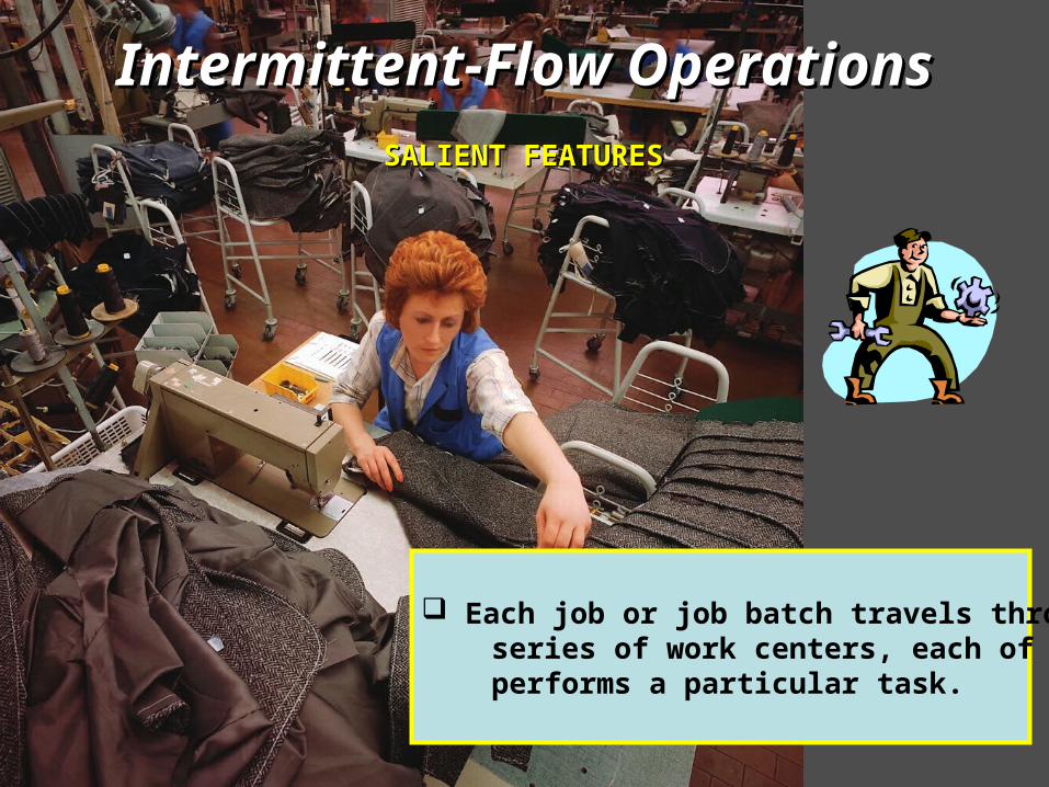
Each job or job batch travels through a series of work centers, each of which performs a particular task.
Intermittent-Flow OperationsIntermittent-Flow Operations
SALIENT FEATURESSALIENT FEATURES

Work centers are grouped by majorprocessing function.
Intermittent-Flow OperationsIntermittent-Flow Operations
SALIENT FEATURESSALIENT FEATURES

Each job or job batch has its own unique route through the system.
Intermittent-Flow OperationsIntermittent-Flow Operations
SALIENT FEATURESSALIENT FEATURES

Intermittent-Flow OperationsIntermittent-Flow Operations
SALIENT FEATURESSALIENT FEATURES
Job processing times at each workcenter are estimated based on similar past jobs and worker
experience

Intermittent-Flow OperationsIntermittent-Flow Operations
Work centers are grouped by function.
Each job or job batch has its own unique route
through the system.
Job processing times at each work center are
estimated based on similar past jobs and worker
experience.
Workers are highly skilled and flexible.
SALIENT FEATURESSALIENT FEATURES
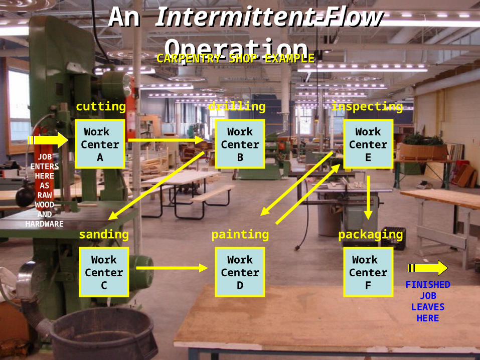
An An Intermittent-Flow Intermittent-Flow OperationOperation
Work Center
A
WorkCenter
B
WorkCenter
E
WorkCenter
C
WorkCenter
D
Work Center
F
cutting drilling inspecting
sanding painting packaging
JOBENTERS
HEREAS
RAWWOODAND
HARDWARE
FINISHEDJOB
LEAVESHERE
CARPENTRY SHOP EXAMPLECARPENTRY SHOP EXAMPLE

Evaluating all incoming jobs to see which workcenters they must pass through in order to
be completed.
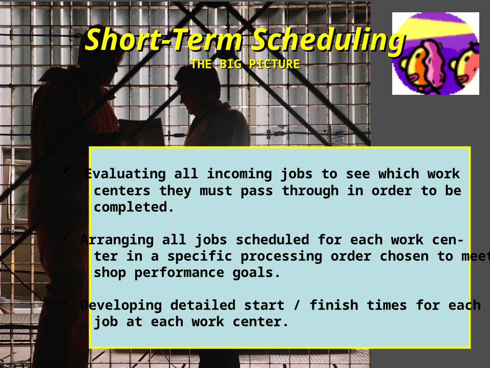
Short-Term SchedulingShort-Term SchedulingTHE BIG PICTURETHE BIG PICTURE

Arranging all jobs scheduled for each work centerin a specific processing order chosen to meet
the shop’s performance goals.
Short-Term SchedulingShort-Term SchedulingTHE BIG PICTURETHE BIG PICTURE
Short-Term SchedulingShort-Term SchedulingTHE BIG PICTURETHE BIG PICTURE
Evaluating all incoming jobs to see which work centers they must pass through in order to be completed.
Arranging all jobs scheduled for each work cen- ter in a specific processing order chosen to meet shop performance goals.
Developing detailed start / finish times for each job at each work center.

Short-Term Scheduling Short-Term Scheduling HistoryHistory
Developed by Henry Gantt, a school teacher by training and later an engineer.
Refined and expanded on the existing body of production
and cost control techniques.
Developed the Gantt Chart in 1914 for scheduling and con-
trolling production and major projects.
Henry Laurence GanttHenry Laurence Gantt1861 - 19191861 - 1919

Gantt Chart Gantt Chart AccomplishmentsAccomplishments
WORLD WAR I NAVAL SHIPS ( 1917 ) HOOVER DAM ( 1931 ) MANHATTAN PROJECT ( 1942 ) INTERSTATE HIGHWAY SYSTEM ( 1956 )
Dr. Robert Oppenheimer and General Kenneth Nichols
THE GANTT CHART WAS THE PRECURSORTHE GANTT CHART WAS THE PRECURSOROF PERT/CPM: TODAY’S POPULAR TECHNIQUEOF PERT/CPM: TODAY’S POPULAR TECHNIQUE
FOR MANAGING MAJOR PROJECTS INFOR MANAGING MAJOR PROJECTS INGOVERNMENT AND INDUSTRYGOVERNMENT AND INDUSTRY

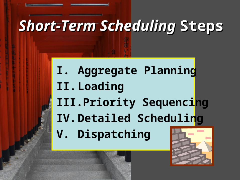
Short-Term Scheduling Short-Term Scheduling StepsSteps
I. Aggregate Planning
II. Loading
III. Priority Sequencing
IV. Detailed Scheduling
V. Dispatching

Aggregate PlanningAggregate Planning
Identify a quasi-unit that best reflects the
firm’s overall output of goods and services
Multiply the quasi-unit forecast by the quasi-
unit resource requirements.
BRIEF REVIEWBRIEF REVIEW
THESE STEPS WILL DETERMINE THE NUMBER AND TYPE OF WORK CENTERS, EQUIPMENT, PERSONNEL, PARTS,
AND SUPPLIES THAT THE FIRM MUST INVEST IN

Number of Vehicles to be Repaired( in quasi-units )
Average Consumption of Resources,Human and Non-Human
( per quasi-unit )
Total Resource RequirementsOver Life of the Aggregate Plan
Number of Mechanics Number of Vehicle Lifts
Size of the Parts Department Number and Types of Equipment
AUTOMOBILEAUTOMOBILEDEALERSHIPDEALERSHIP
REPAIR FACILITYREPAIR FACILITYEXAMPLEEXAMPLE

Short-Term Scheduling Short-Term Scheduling StepsSteps
I. Aggregate Planning
II. Loading
III. Priority Sequencing
IV. Detailed Scheduling
V. Dispatching

LOADINGLOADING
ALSO KNOWN AS SHOPLOADING or MACHINE LOADING
The assignment and commitmentof arriving jobs to one or more
work centers for the day, week, ormonth, based on job needs.

Gantt Chart for LoadingGantt Chart for Loading
WEEKLY SCHEDULE – DEPARTMENT 3985: MODEL SHOP SCHEDULE 3/16 - 22WEEKLY SCHEDULE – DEPARTMENT 3985: MODEL SHOP SCHEDULE 3/16 - 22
WORKWORK
CENTERCENTERMONMON TUESTUES WEDWED THURTHUR FRIFRI SATSAT
Machining
Fabrication
Assembly
Testing
Packaging
D
D
D
D
A
B
B
B
C
C
C
E
E
E
F
F
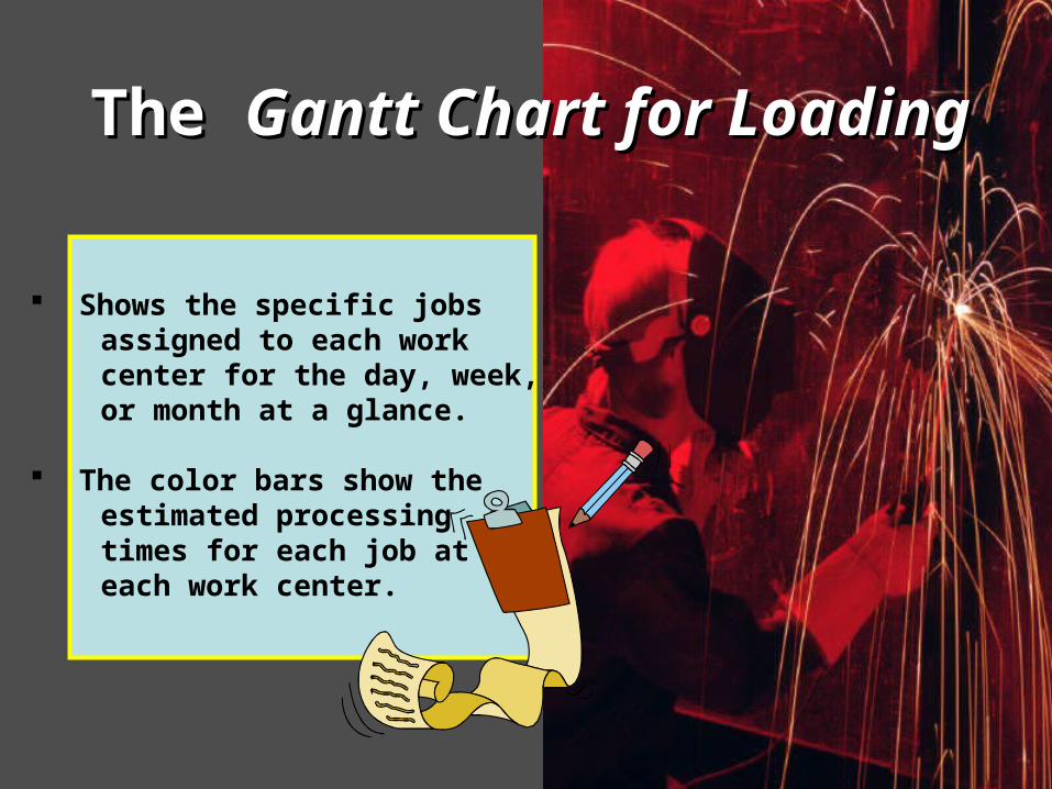
The The Gantt Chart for LoadingGantt Chart for Loading
Shows the specific jobs assigned to each work center for the day, week, or month at a glance.
The color bars show the estimated processing times for each job at each work center.

The The Gantt Chart for LoadingGantt Chart for Loading
Does not show the exact start and finish times for each job at each center.
Does not show the exact order in which each job will be processed at each center.
Short-Term Scheduling Short-Term Scheduling StepsSteps
I. Aggregate Planning
II. Loading
III. Priority Sequencing
IV. Detailed Scheduling
V. Dispatching

PRIORITY SEQUENCINGPRIORITY SEQUENCING
THE ORDER IN WHICH JOBSWAITING AT EACH WORK
CENTER WILL BEPROCESSED
THE ORDER OF PROCESSING SELECTED WILL BEST MEETMANAGEMENT’S SHOP GOALS
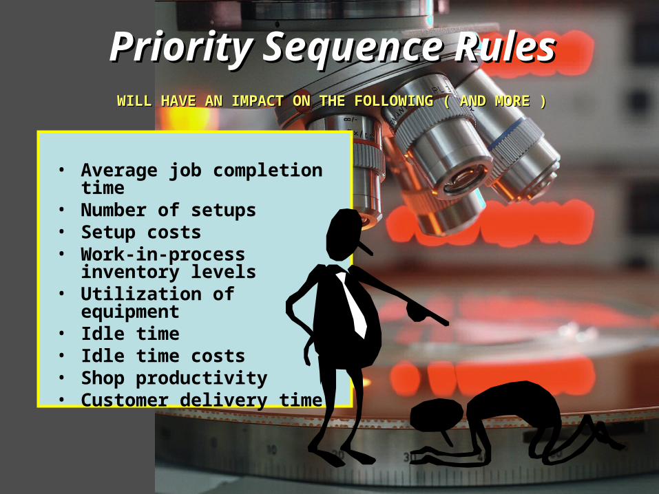
Priority Sequence RulesPriority Sequence Rules
• Average job completion time
• Number of setups• Setup costs• Work-in-process inventory
levels• Utilization of equipment• Idle time• Idle time costs• Shop productivity• Customer delivery time
WILL HAVE AN IMPACT ON THE FOLLOWING ( AND MORE )WILL HAVE AN IMPACT ON THE FOLLOWING ( AND MORE )

A Few A Few Priority Sequence Priority Sequence RulesRulesOVER 36 TO CHOOSE FROMOVER 36 TO CHOOSE FROM
• SPTSPT shortest processing time
• FIFOFIFO first in - first out
• LIFOLIFO last in - first out
• SSSS static slack
• CRCR critical ratio
• FISFSFISFS first in system - first served
( ALSO KNOWN AS DD , DUE DATE )

Priority Sequence RulesPriority Sequence RulesNEW PERFORMANCE CRITERIANEW PERFORMANCE CRITERIA
1. Average job completion time2. Labor or machine utilization3. Average number of jobs in the system4. Average number of late days per job
We evaluate priority sequencerules using one or more of the
following criteria:

Possible Job Shop GoalsPossible Job Shop Goals
Internal Shop Efficiency
Customer Service
Mix of Both
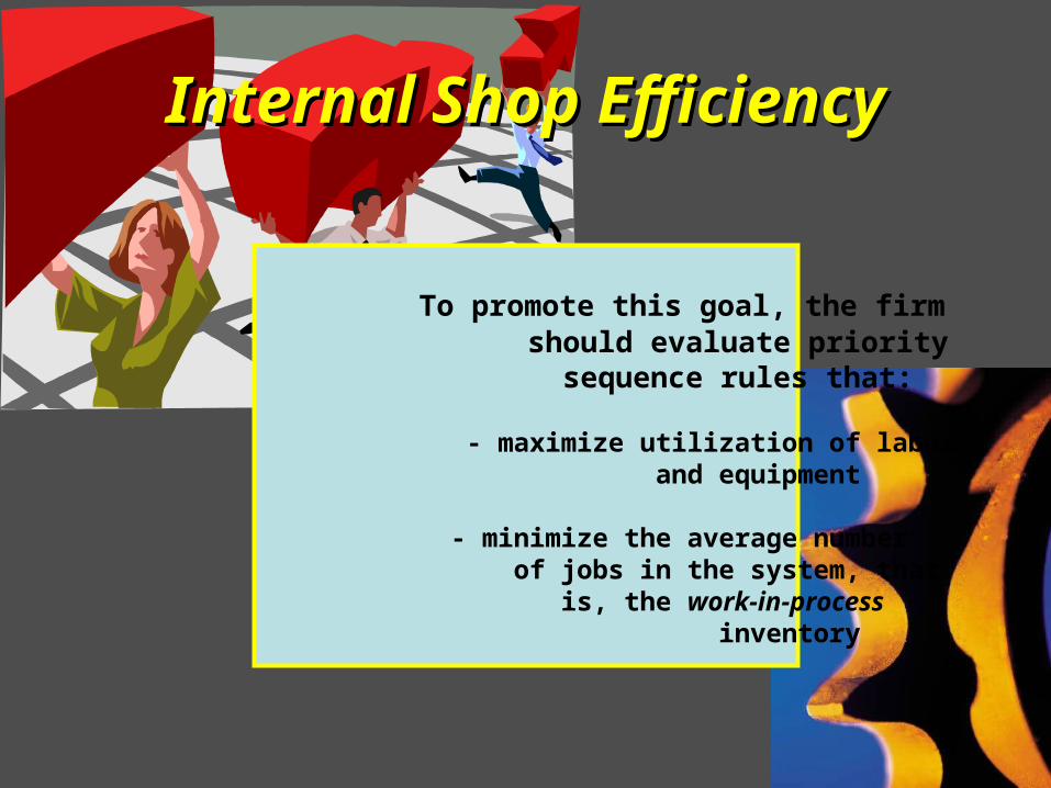
Internal Shop EfficiencyInternal Shop Efficiency
To promote this goal, the firm should evaluate priority sequence rules that: - maximize utilization of labor and equipment
- minimize the average number of jobs in the system, that is, the work-in-process inventory

Customer ServiceCustomer Service
To promote this goal, the firm
should evaluate priority
sequence rules that:
- minimize average job lateness ( tardiness )
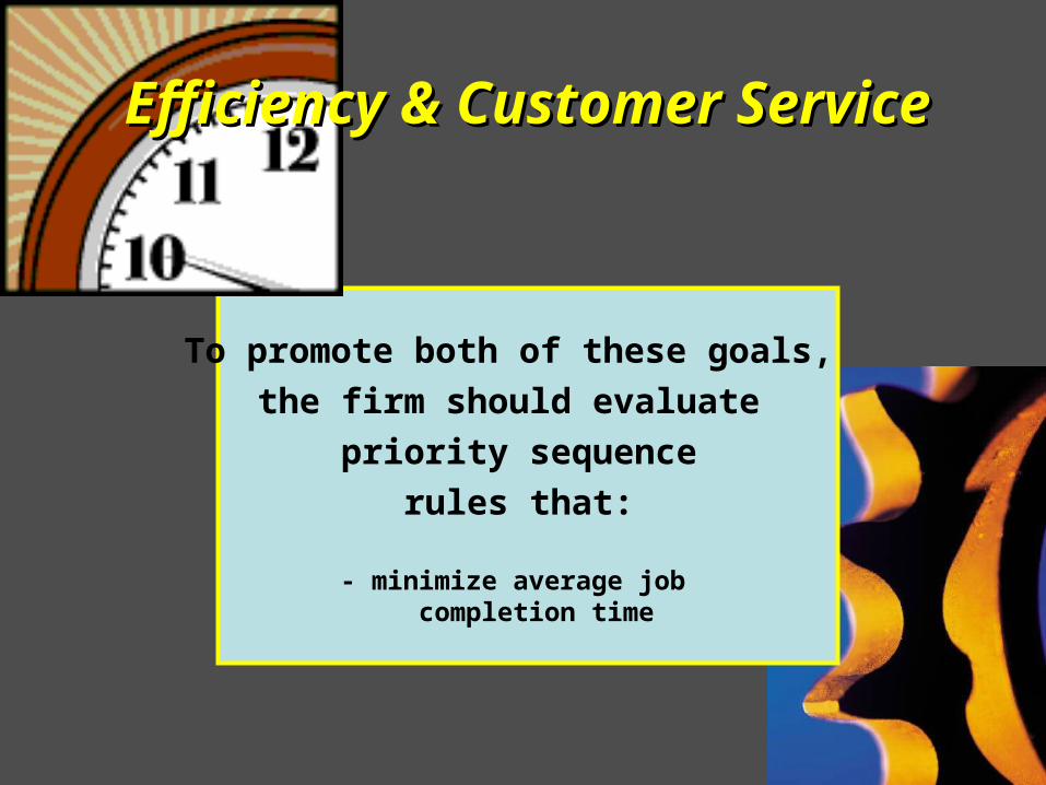
Efficiency & Customer ServiceEfficiency & Customer Service
To promote both of these goals,
the firm should evaluate
priority sequence
rules that:
- minimize average job completion time

There are currently about a dozen priority sequence rules that support the goal of internal shop efficiency.
We evaluate those dozen rules using two particular performance criteria only. 1. “MAXIMIZE UTILIZATION of workers and equipment” 2. “MINIMIZE WORK-in-PROCESS INVENTORY” We select the rule that best satisfies those two criteria.
TheTheconnectionconnection
betweenbetweenshop goalsshop goals
andandprioritypriority
sequencesequencerulesrules

There are currently about a dozen priority sequence rules that support the goal of customer service.
We evaluate those dozen rules using one particular performance criterion only: “MINIMIZE JOB LATENESS”
We select the rule that best satisfies that criterion.
TheTheconnectionconnection
betweenbetweenshop goalsshop goals
andandprioritypriority
sequencesequencerulesrules
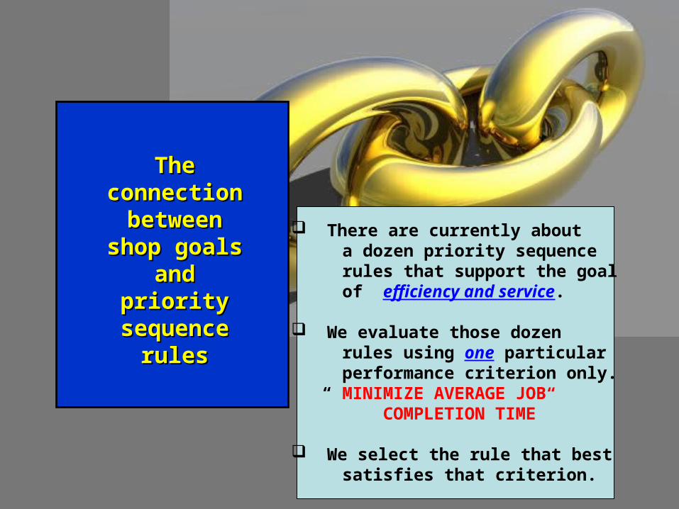
There are currently about a dozen priority sequence rules that support the goal of efficiency and service.
We evaluate those dozen rules using one particular performance criterion only. “ MINIMIZE AVERAGE JOB COMPLETION TIME”
We select the rule that best satisfies that criterion.
TheTheconnectionconnection
betweenbetweenshop goalsshop goals
andandprioritypriority
sequencesequencerulesrules

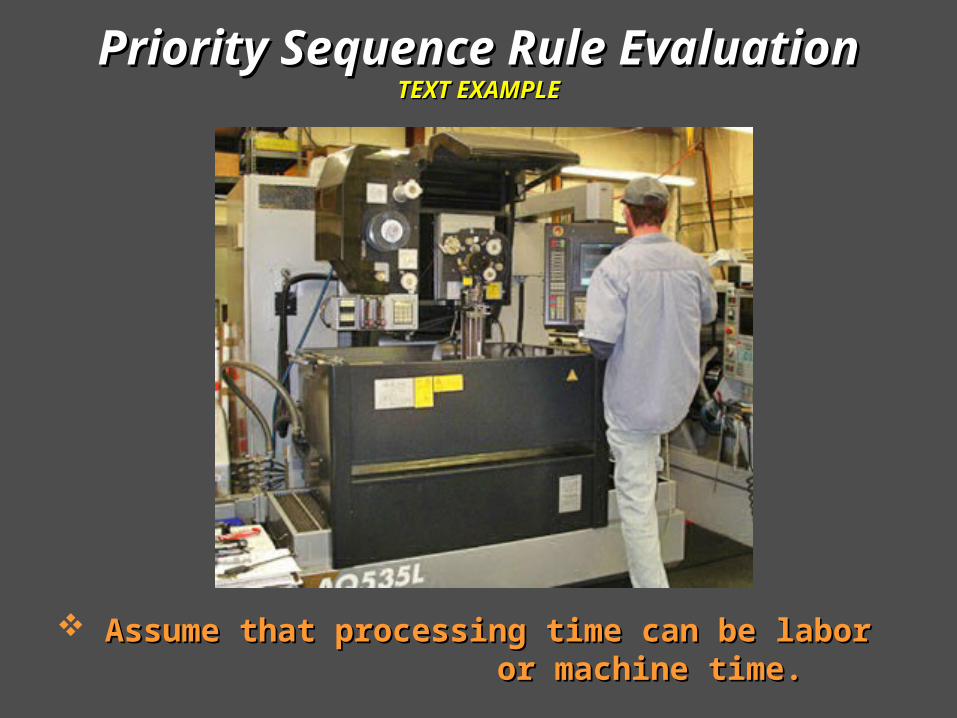
Priority Sequence Rule EvaluationPriority Sequence Rule EvaluationTEXT EXAMPLETEXT EXAMPLE
Assume that this job shop has only one work center.Assume that this job shop has only one work center.

Priority Sequence Rule EvaluationPriority Sequence Rule EvaluationTEXT EXAMPLETEXT EXAMPLE
Assume that this work center can only process one Assume that this work center can only process one job at a time.job at a time.
Priority Sequence Rule EvaluationPriority Sequence Rule EvaluationTEXT EXAMPLETEXT EXAMPLE
Assume that processing time can be labor Assume that processing time can be labor or machine time.or machine time.

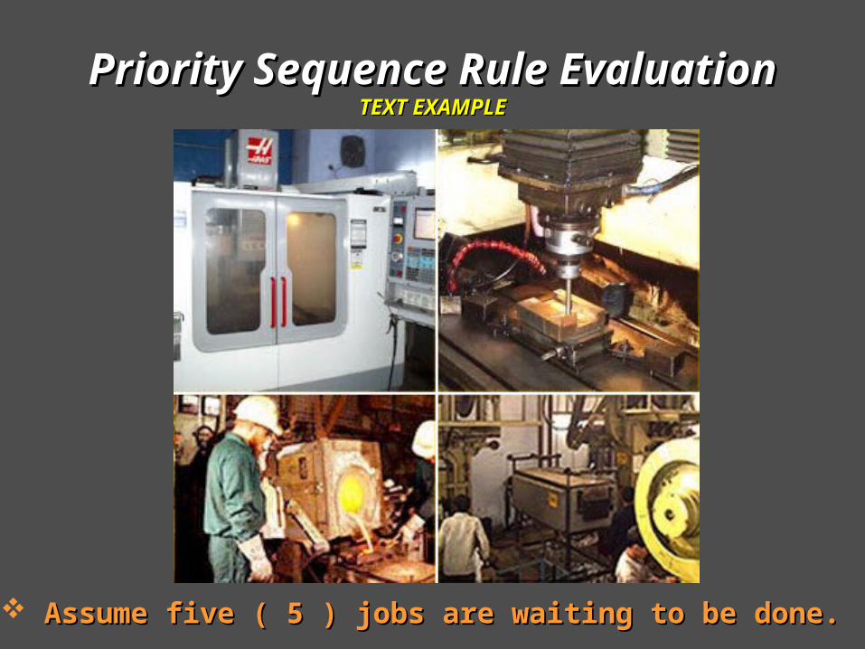
Priority Sequence Rule EvaluationPriority Sequence Rule EvaluationTEXT EXAMPLETEXT EXAMPLE
Assume it is the 1Assume it is the 1stst day of the month. day of the month.
Priority Sequence Rule EvaluationPriority Sequence Rule EvaluationTEXT EXAMPLETEXT EXAMPLE
Assume five ( 5 ) jobs are waiting to be done.Assume five ( 5 ) jobs are waiting to be done.

Priority Sequence Rule ExamplePriority Sequence Rule ExampleTHE FIVE JOBS THE FIVE JOBS
JOBSJOB
PROCESS TIMES
JOB
DEADLINES( tentative )
A 5 Days 10th Day
B 10 Days 15th Day
C 2 Days 5th Day
D 8 Days 12th Day
E 6 Days 8th Day

Shortest Processing Time Shortest Processing Time (SPT)(SPT)THE JOB PROCESSING ORDERTHE JOB PROCESSING ORDER
JOB PROCESSJOB PROCESS
ORDERORDER
JOB PROCESSJOB PROCESS
TIMETIME
COMPLETIONCOMPLETION
TIME TIME
JOB DEADLINEJOB DEADLINE( tentative )( tentative )
JOBJOB
LATENESSLATENESS
C 2 Days 2nd Day 5th Day 0 Days
A 5 Days 7th Day 10th Day 0 Days
E 6 Days 13th Day 8th Day 5 Days
D 8 Days 21st Day 12th Day 9 Days
B 10 Days 31st Day 15th Day 16 Days
5 Jobs 31 Days 74 Days - 30 Days
11
Completion TimeCompletion Time, or , or Flow TimeFlow Time = Job Waiting Time + Job Processing Time = Job Waiting Time + Job Processing Time
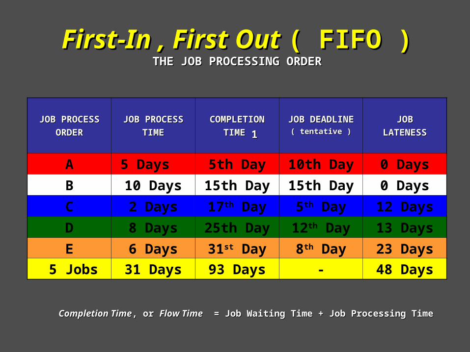
First-In , First Out First-In , First Out ( FIFO )( FIFO )THE JOB PROCESSING ORDERTHE JOB PROCESSING ORDER
JOB PROCESSJOB PROCESS
ORDERORDER
JOB PROCESSJOB PROCESS
TIMETIME
COMPLETIONCOMPLETION
TIME TIME
JOB DEADLINEJOB DEADLINE( tentative )( tentative )
JOBJOB
LATENESSLATENESS
A 5 Days 5th Day 10th Day 0 Days
B 10 Days 15th Day 15th Day 0 Days
C 2 Days 17th Day 5th Day 12 Days
D 8 Days 25th Day 12th Day 13 Days
E 6 Days 31st Day 8th Day 23 Days
11
5 Jobs 31 Days 93 Days - 48 Days
Completion TimeCompletion Time, or , or Flow TimeFlow Time = Job Waiting Time + Job Processing Time = Job Waiting Time + Job Processing Time

First-in-System , First-Served First-in-System , First-Served (FSFS)(FSFS)JOBS ARE LINED UP BY JOBS ARE LINED UP BY DUE DATEDUE DATE
JOB PROCESSJOB PROCESS
ORDERORDER
JOB PROCESSJOB PROCESS
TIMETIME
COMPLETIONCOMPLETION
TIME TIME
JOB DEADLINEJOB DEADLINE( tentative )( tentative )
JOBJOB
LATENESSLATENESS
C 2 Days 2nd Day 5th Day 0 Days
E 6 Days 8th Day 8th Day 0 Days
A 5 Days 13th Day 10th Day 3 Days
D 8 Days 21st Day 12th Day 9 Days
B 10 Days 31st Day 15th Day 16 Days
5 Jobs 31 Days 75 Days - 28 Days
11
Completion TimeCompletion Time, or , or Flow TimeFlow Time = Job Waiting Time + Job Processing Time = Job Waiting Time + Job Processing Time

Static Slack Static Slack ComputationsComputations
JOB DEADLINE DATE – CURRENT DATE – JOB PROCESS TIMEJOB DEADLINE DATE – CURRENT DATE – JOB PROCESS TIME
JOB A : 10th day – 1st day – 5 days = 4 days
JOB B : 15th day – 1st day – 10 days = 4 days
JOB C : 5th day – 1st day – 2 days = 2 days
JOB D : 12th day – 1st day – 8 days = 3 days
JOB E : 8th day – 1st day – 6 days = 1 day
THE JOB WITH THE SMALLEST
STATIC SLACK IS DONEFIRST

JOB PROCESSJOB PROCESS
ORDERORDER
JOB PROCESSJOB PROCESS
TIMETIME
COMPLETIONCOMPLETION
TIME TIME
JOB DEADLINEJOB DEADLINE( tentative )( tentative )
JOBJOB
LATENESSLATENESS
E 6 Days 6th Day 8th Day 0 Days
C 2 Days 8th Day 5th Day 3 Days
D 8 Days 16th Day 12th Day 4 Days
A 5 Days 21st Day 10th Day 11 Days
B 10 Days 31st Day 15th Day 16 Days
5 Jobs 31 Days 82 Days - 34 Days
11
Static Slack - Static Slack - (( SS )SS )
Completion TimeCompletion Time, or , or Flow TimeFlow Time = Job Waiting Time + Job Processing Time = Job Waiting Time + Job Processing Time
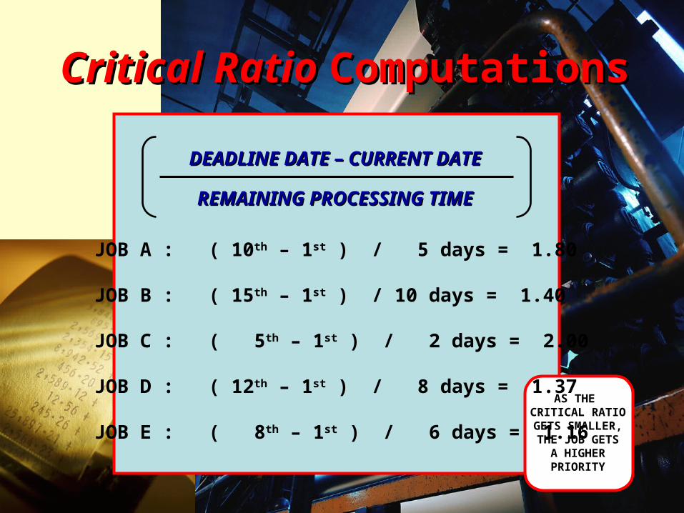
Critical Ratio Critical Ratio ComputationsComputations
DEADLINE DATE – CURRENT DATEDEADLINE DATE – CURRENT DATE
REMAINING PROCESSING TIMEREMAINING PROCESSING TIME
JOB A : ( 10th – 1st ) / 5 days = 1.80
JOB B : ( 15th – 1st ) / 10 days = 1.40
JOB C : ( 5th – 1st ) / 2 days = 2.00
JOB D : ( 12th – 1st ) / 8 days = 1.37
JOB E : ( 8th – 1st ) / 6 days = 1.16
AS THE CRITICAL RATIOGETS SMALLER,THE JOB GETS
A HIGHERPRIORITY
JOB PROCESS
ORDER
JOB PROCESS
TIME
COMPLETION
TIME
JOB DEADLINE( tentative )
JOB
LATENESS
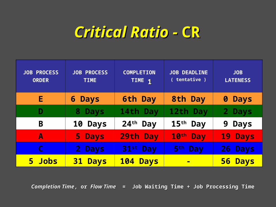
E 6 Days 6th Day 8th Day 0 Days
D 8 Days 14th Day 12th Day 2 Days
B 10 Days 24th Day 15th Day 9 Days
A 5 Days 29th Day 10th Day 19 Days
C 2 Days 31st Day 5th Day 26 Days
5 Jobs 31 Days 104 Days - 56 Days
11
Critical Ratio - Critical Ratio - CRCR
Completion TimeCompletion Time, or , or Flow TimeFlow Time = Job Waiting Time + Job Processing Time = Job Waiting Time + Job Processing Time
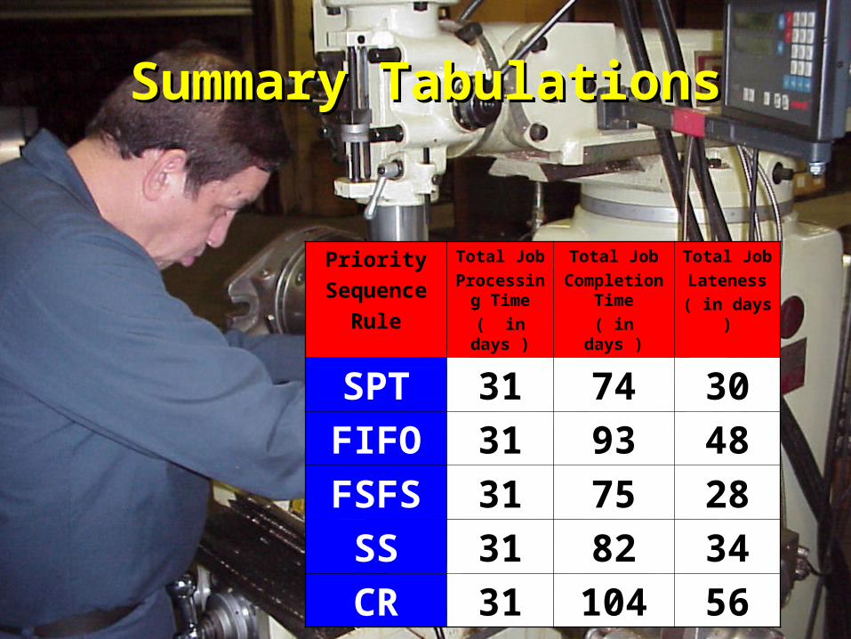
Summary TabulationsSummary Tabulations
Priority
Sequence
Rule
Total Job
Processing Time
( in days )
Total Job
Completion Time
( in days )
Total Job
Lateness
( in days )
SPT 31 74 30
FIFO 31 93 48
FSFS 31 75 28
SS 31 82 34
CR 31 104 56

Average Job Completion TimeAverage Job Completion Time
Total Flow Time / Number of JobsTotal Flow Time / Number of Jobs
SPT Rule 74 days / 5 jobs = 14.8 days
FIFO Rule 93 days / 5 jobs = 18.6 days
FSFS (DD) 75 days / 5 jobs = 15.0 days
STATIC SLACK 82 days / 5 Jobs = 16.4 days
CRITICAL RATIO 104 days / 5 Jobs = 20.8 days

Labor / Machine UtilizationLabor / Machine Utilization
Total Processing Time / Total Flow TimeTotal Processing Time / Total Flow Time
SPT Rule 31 days / 74 days = 42.00%
FIFO Rule 31 days / 93 days = 33.3%
FSFS (DD) 31 days / 75 days = 41.33%
STATIC SLACK 31 days / 82 days = 37.8%
CRITICAL RATIO 31 days / 104 days = 29.81%

Average Number of Jobs in the SystemAverage Number of Jobs in the System
Total Flow Time / Total Processing TimeTotal Flow Time / Total Processing Time
SPT Rule 74 days / 31 days = 2.39 jobs
FIFO Rule 93 days / 31 days = 3.0 jobs
FSFS (DD) 75 days / 31 days = 2.42 jobs
STATIC SLACK 82 days / 31 days = 2.65 jobs
CRITICAL RATIO 104 days / 31 days = 3.35 jobs

Average Number of Late Days per JobAverage Number of Late Days per Job
SPT Rule 30 days / 5 jobs = 6.0 days
FIFO Rule 48 days / 5 jobs = 9.6 days
FSFS ( DD ) 28 days / 5 jobs = 5.6 days
STATIC SLACK 34 days / 5 jobs = 6.8 days
CRITICAL RATIO 56 days / 5 jobs = 11.2 days
Total Late Days / Number of JobsTotal Late Days / Number of Jobs

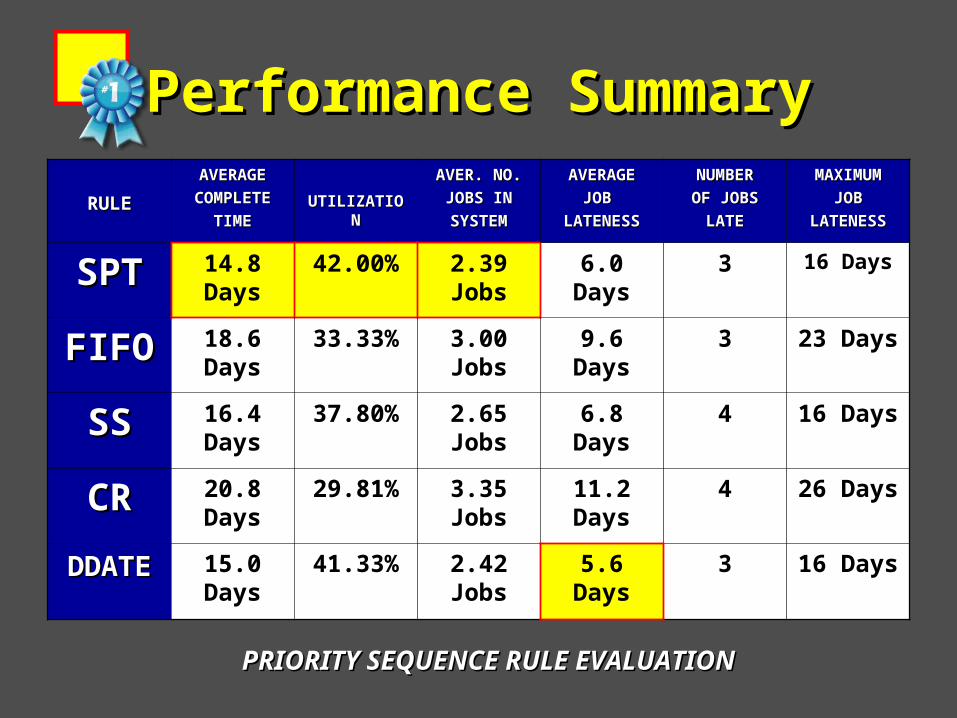
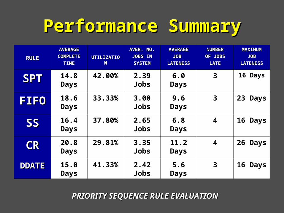
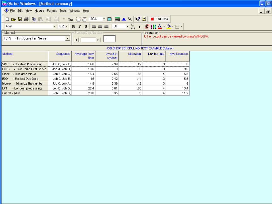
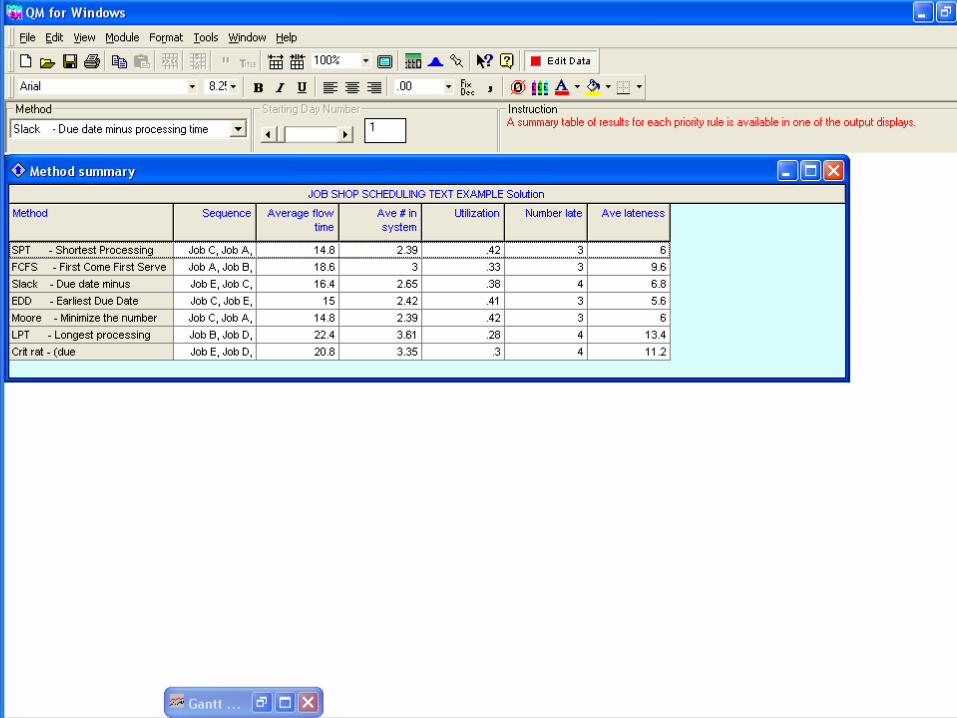
Performance SummaryPerformance Summary
RULERULE
AVERAGEAVERAGE
COMPLETECOMPLETE
TIMETIMEUTILIZATIONUTILIZATION
AVER. NO.AVER. NO.
JOBS INJOBS IN
SYSTEMSYSTEM
AVERAGEAVERAGE
JOB JOB
LATENESSLATENESS
NUMBERNUMBER
OF JOBSOF JOBS
LATELATE
MAXIMUMMAXIMUM
JOBJOB
LATENESSLATENESS
SPTSPT 14.8 Days
42.00% 2.39 Jobs
6.0 Days 3 16 Days
FIFOFIFO 18.6 Days
33.33% 3.00 Jobs
9.6 Days 3 23 Days
SSSS 16.4 Days
37.80% 2.65 Jobs
6.8 Days 4 16 Days
CRCR 20.8 Days
29.81% 3.35 Jobs
11.2 Days
4 26 Days
DDATEDDATE 15.0 Days
41.33% 2.42 Jobs
5.6 Days 3 16 Days
PRIORITY SEQUENCE RULE EVALUATIONPRIORITY SEQUENCE RULE EVALUATION

Postscript
The SPT rule always minimizes average job completion time ( flow time ) and the average number of jobs in the system..

Postscript
The DDATE rule always minimizes average job lateness and total job lateness.

Postscript
FIFO ( FCFS ) does not score well on most criteria but neither does it score poorly. It does however appear fair to customers which is important in service sector systems.

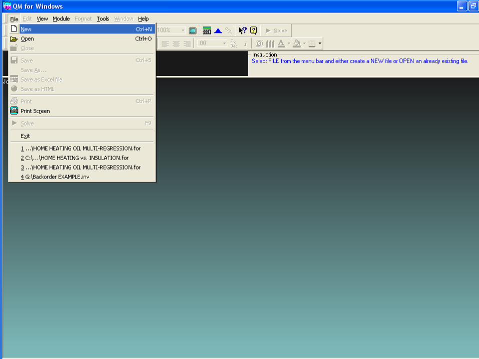
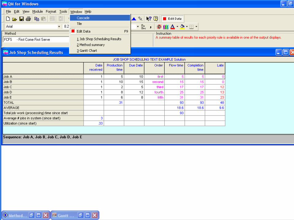
Job Shop w / QMJob Shop w / QM forfor WindowsWindows

We Scroll To
JOB SHOP SCHEDULING

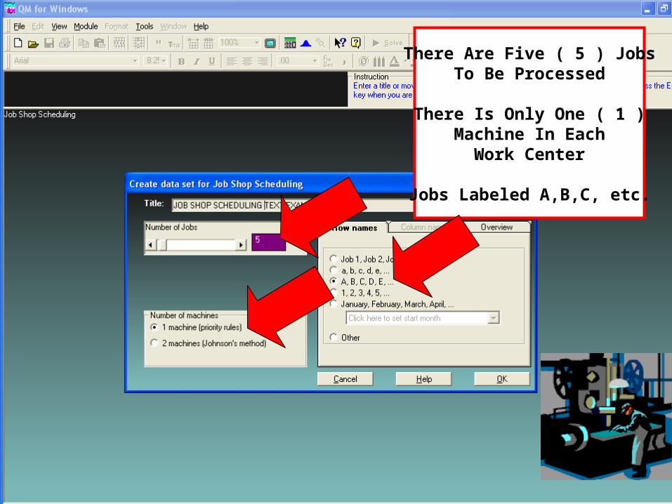
There Are Five ( 5 ) JobsTo Be Processed
There Is Only One ( 1 )Machine In Each
Work Center
Jobs Labeled A,B,C, etc.
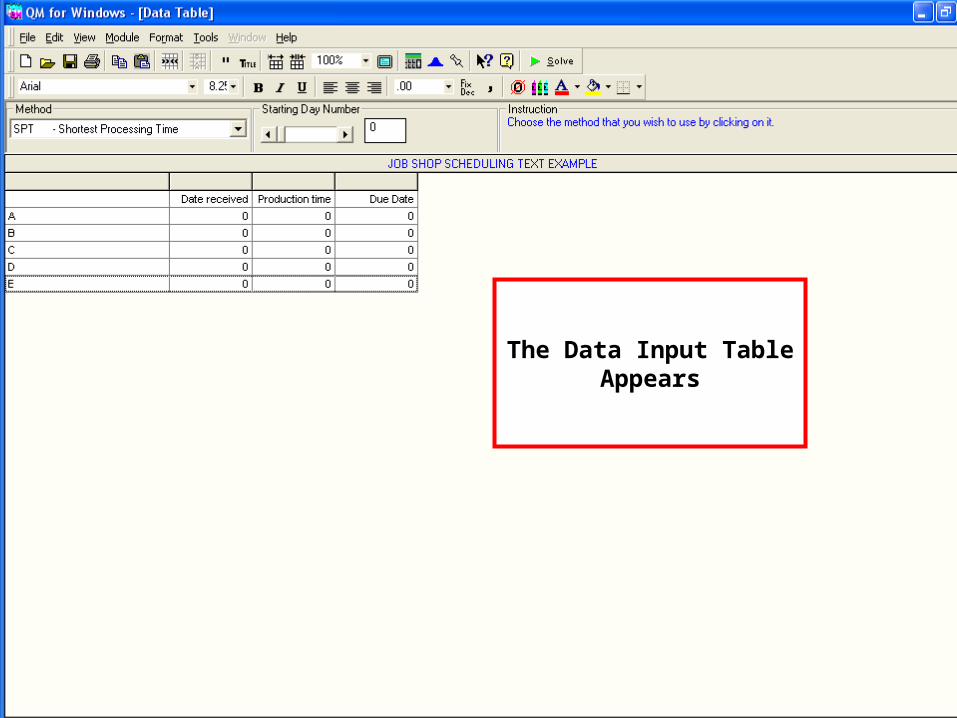
The Data Input TableAppears

We Schedule Under TheSPT
Priority Sequence Rule.
It is the 1st Day of the Month.
Estimated Processing TimesAre Entered Under“ Production Time”
&Job Deadlines Are
Entered Under“Due Date”
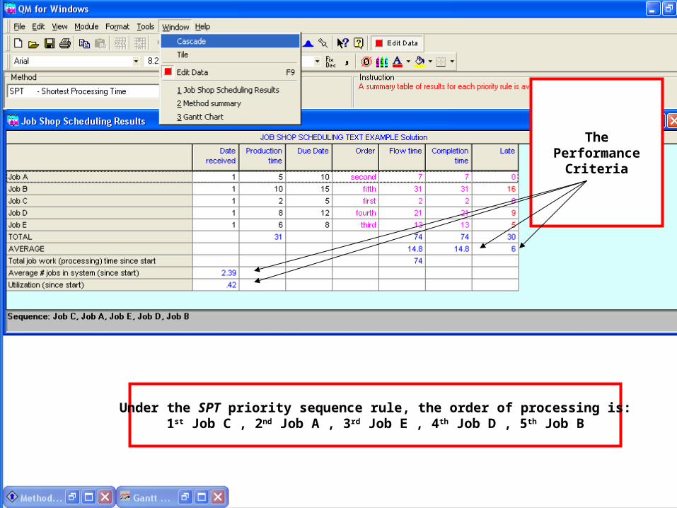
Under the SPT priority sequence rule, the order of processing is:1st Job C , 2nd Job A , 3rd Job E , 4th Job D , 5th Job B
ThePerformance
Criteria
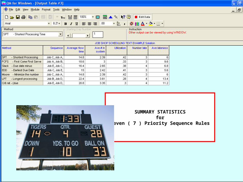
SUMMARY STATISTICSfor
Seven ( 7 ) Priority Sequence Rules
Performance SummaryPerformance Summary
RULERULE
AVERAGEAVERAGE
COMPLETECOMPLETE
TIMETIMEUTILIZATIONUTILIZATION
AVER. NO.AVER. NO.
JOBS INJOBS IN
SYSTEMSYSTEM
AVERAGEAVERAGE
JOB JOB
LATENESSLATENESS
NUMBERNUMBER
OF JOBSOF JOBS
LATELATE
MAXIMUMMAXIMUM
JOBJOB
LATENESSLATENESS
SPTSPT 14.8 Days
42.00% 2.39 Jobs
6.0 Days 3 16 Days
FIFOFIFO 18.6 Days
33.33% 3.00 Jobs
9.6 Days 3 23 Days
SSSS 16.4 Days
37.80% 2.65 Jobs
6.8 Days 4 16 Days
CRCR 20.8 Days
29.81% 3.35 Jobs
11.2 Days
4 26 Days
DDATEDDATE 15.0 Days
41.33% 2.42 Jobs
5.6 Days 3 16 Days
PRIORITY SEQUENCE RULE EVALUATIONPRIORITY SEQUENCE RULE EVALUATION

The Gantt Loading Chart for
One ( 1 ) Work Center
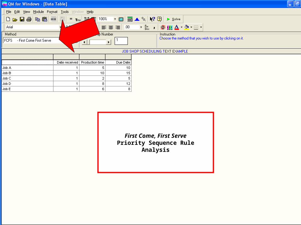
First Come, First ServePriority Sequence Rule
Analysis


Earliest Due DatePriority Sequence Rule
Analysis


Static Slack Priority Sequence Rule
Analysis


Critical RatioPriority Sequence Rule
Analysis


Short-Term Scheduling Short-Term Scheduling StepsSteps
I. Aggregate Planning
II. Loading
III. Priority Sequencing
IV. Detailed Scheduling
V. Dispatching
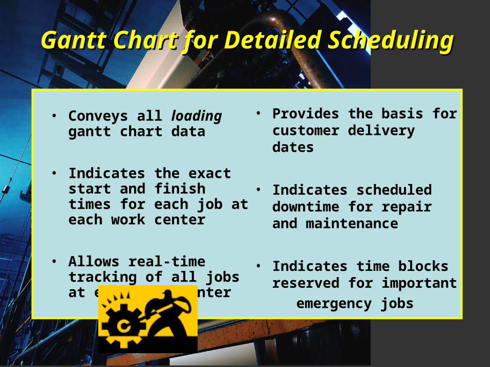
Gantt Chart for Detailed SchedulingGantt Chart for Detailed Scheduling
• Conveys all loading gantt chart data
• Indicates the exact start and finish times for each job at each work center
• Allows real-time tracking of all jobs at each work center
• Provides the basis for customer delivery dates
• Indicates scheduled downtime for repair and maintenance
• Indicates time blocks reserved for important
emergency jobs
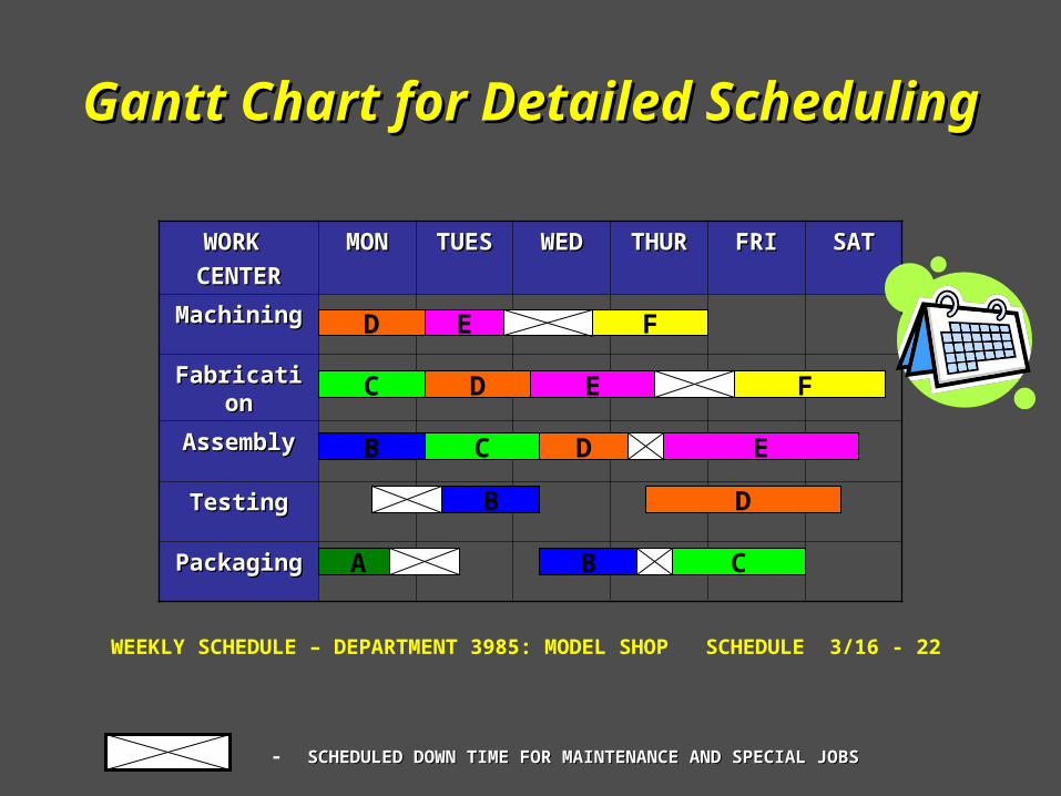
Gantt Chart for Detailed SchedulingGantt Chart for Detailed Scheduling
WEEKLY SCHEDULE – DEPARTMENT 3985: MODEL SHOP SCHEDULE 3/16 - 22
WORK WORK
CENTERCENTER
MONMON TUESTUES WEDWED THURTHUR FRIFRI SATSAT
MachiningMachining
FabricationFabrication
AssemblyAssembly
TestingTesting
PackagingPackaging
D
D
D
D
A
B
B
B
C
C
C
E
E
E
F
F
- SCHEDULED DOWN TIME FOR MAINTENANCE AND SPECIAL JOBSSCHEDULED DOWN TIME FOR MAINTENANCE AND SPECIAL JOBS
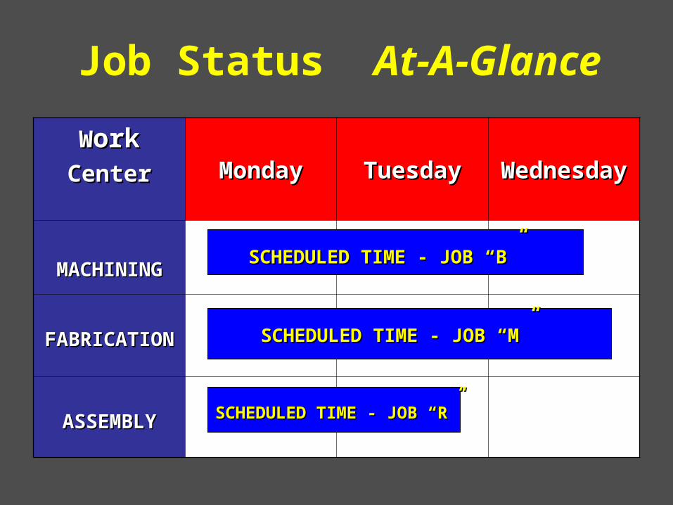
Job Status At-A-Glance
WWorkorkCenterCenter MondayMonday TuesdayTuesday WednesdayWednesday
MACHININGMACHINING
FABRICATIONFABRICATION
ASSEMBLYASSEMBLY
SCHEDULED TIME - JOB “B”SCHEDULED TIME - JOB “B”
SCHEDULED TIME - JOB “M”SCHEDULED TIME - JOB “M”
SCHEDULED TIME - JOB “R”SCHEDULED TIME - JOB “R”

Job Status Job Status At-A-GlanceAt-A-Glance
WWorkorkCenterCenter MondayMonday TuesdayTuesday WednesdayWednesday
MACHININGMACHINING
FABRICATIONFABRICATION
ASSEMBLYASSEMBLY
CURSOR DENOTES REAL TIMECURSOR DENOTES REAL TIME
ACTUAL PROGRESS
ACTUAL PROGRESS
ACTUAL PROGRESS
JOB B
JOB M
JOB R
SCHEDULED TIME
SCHEDULED TIME
SCHEDULED TIME
JOB B IS BEHIND SCHEDULE AS OF LATE MORNING TUESDAY

Job Status At-A-Glance
WWorkorkCenterCenter MondayMonday TuesdayTuesday WednesdayWednesday
MACHININGMACHINING
FABRICATIONFABRICATION
ASSEMBLYASSEMBLY
CURSOR DENOTES REAL TIMECURSOR DENOTES REAL TIME
ACTUAL PROGRESS
ACTUAL PROGRESS
ACTUAL PROGRESS
JOB B
JOB M
JOB R
SCHEDULED TIME
SCHEDULED TIME
SCHEDULED TIME
JOB M IS AHEAD OF SCHEDULE AS OF LATE MORNING TUESDAY

Job Status Job Status At-A-GlanceAt-A-Glance
WWorkorkCenterCenter MondayMonday TuesdayTuesday WednesdayWednesday
MACHININGMACHINING
FABRICATIONFABRICATION
ASSEMBLYASSEMBLY
CURSOR DENOTES REAL TIMECURSOR DENOTES REAL TIME
ACTUAL PROGRESS
ACTUAL PROGRESS
ACTUAL PROGRESS
JOB B
JOB M
JOB R
SCHEDULED TIME
SCHEDULED TIME
SCHEDULED TIME
JOB R IS EXACTLY ON SCHEDULE AS OF LATE MORNING TUESDAY

Short-Term Scheduling Short-Term Scheduling StepsSteps
I. Aggregate Planning
II. Loading
III. Priority Sequencing
IV. Detailed Scheduling
V. Dispatching

DispatchingDispatchingThe formal release of the completed job to the customerThe formal release of the completed job to the customer
by the last work center that processed it. by the last work center that processed it.

Short-Term SchedulingShort-Term SchedulingTacticsTactics
Applied Management Science for Decision Making, 1e Applied Management Science for Decision Making, 1e © 2012 Pearson Prentice-Hall, Inc. Philip A. Vaccaro , PhD© 2012 Pearson Prentice-Hall, Inc. Philip A. Vaccaro , PhD

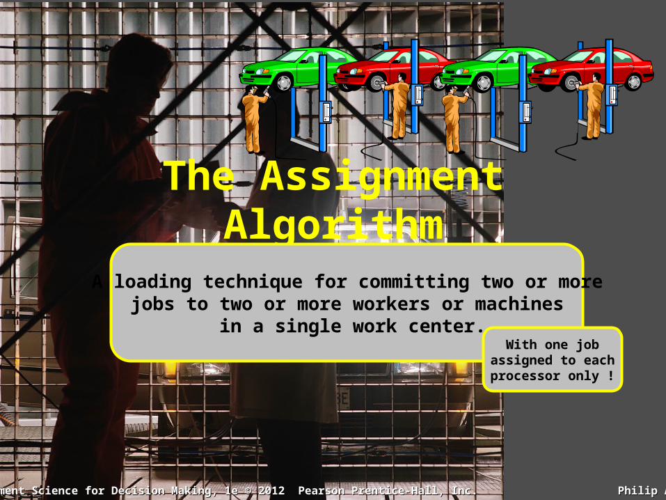
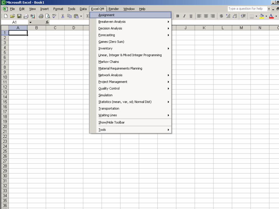
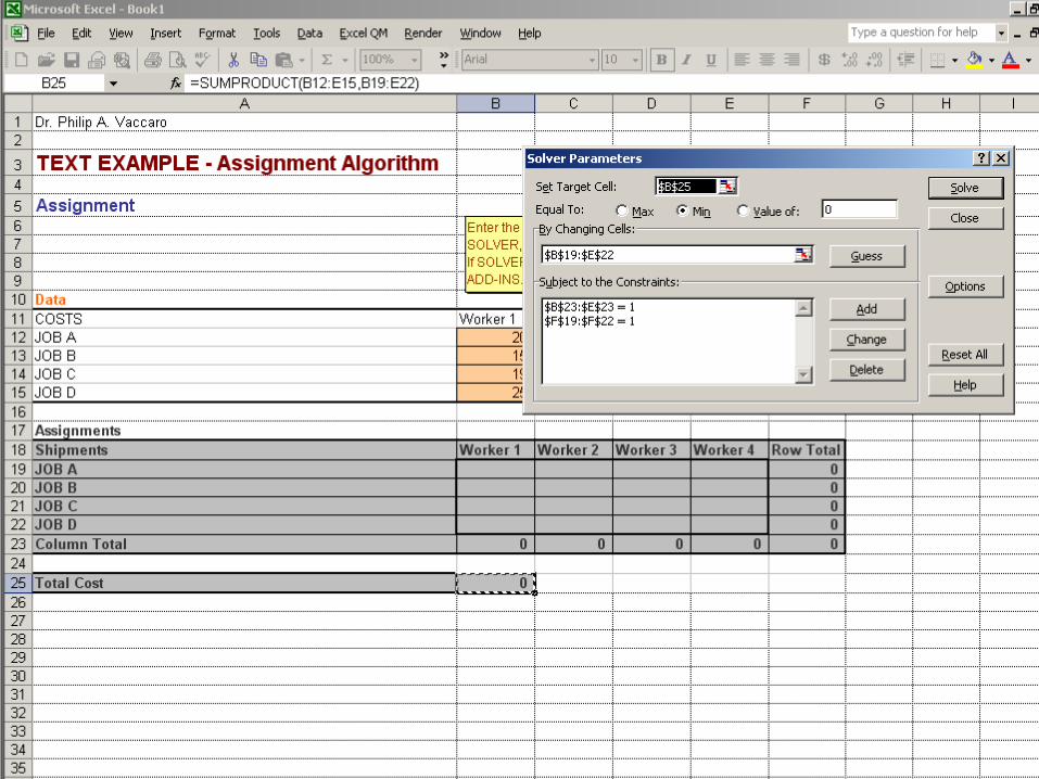
The Assignment Algorithm
A loading technique for committing two or morejobs to two or more workers or machines
in a single work center.With one job
assigned to eachprocessor only !
Applied Management Science for Decision Making, 1e Applied Management Science for Decision Making, 1e © 2012 Pearson Prentice-Hall, Inc. Philip A. Vaccaro , PhD© 2012 Pearson Prentice-Hall, Inc. Philip A. Vaccaro , PhD

CharacteristicsCharacteristics
Streamlined version ofStreamlined version of the the transportation algorithmtransportation algorithm

A Transportation Algorithm Tableau A Transportation Algorithm Tableau
Warehouse
1
Warehouse 2
Warehouse 3
Factory
A
Factory
B
Factory
C
33
$3
$4
$9
$7
$12 $15
$17
$8
$5
FromTo
1
1
1
1 1 1Demand
Availability
ONE UNIT SHIPPED FROM EACH SOURCE - ONE UNIT RECEIVED AT EACH DESTINATIONONE UNIT SHIPPED FROM EACH SOURCE - ONE UNIT RECEIVED AT EACH DESTINATION
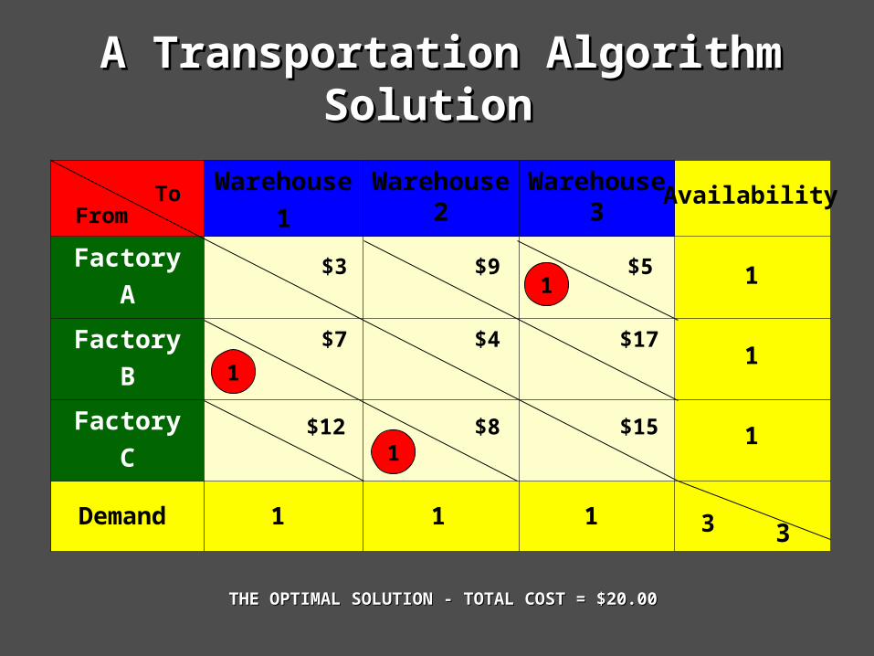
A Transportation Algorithm Solution A Transportation Algorithm Solution
Warehouse
1
Warehouse 2
Warehouse 3
Factory
A
Factory
B
Factory
C
33
$3
$4
$9
$7
$12 $15
$17
$8
$5
FromTo
1
1
1
1 1 1Demand
Availability
1
1
1
THE OPTIMAL SOLUTION - TOTAL COST = $20.00THE OPTIMAL SOLUTION - TOTAL COST = $20.00

An Assignment Algorithm TableauAn Assignment Algorithm Tableau
Warehouse
1
Warehouse 2
Warehouse 3
Factory
A
Factory
B
Factory
C
$3
$4
$9
$7
$12 $15
$17
$8
$5
FromTo
THE “THE “DEMANDDEMAND “ ROW & “ “ ROW & “AVAILABILITY AVAILABILITY ” COLUMN ARE ELIMINATED” COLUMN ARE ELIMINATED

An Assignment Algorithm TableauAn Assignment Algorithm Tableau
Worker
1
Worker
2
Worker
3
Job
A
Job
B
Job
C
$3
$4
$9
$7
$12 $15
$17
$8
$5
FromTo
SHOWS ONLY THE COSTS OF PERFORMING EACH JOB UNDER EACH WORKERSHOWS ONLY THE COSTS OF PERFORMING EACH JOB UNDER EACH WORKER ASSIGNABLE JOBS AND WORKERS CAN REPLACE FACTORIES AND WAREHOUSES ASSIGNABLE JOBS AND WORKERS CAN REPLACE FACTORIES AND WAREHOUSES
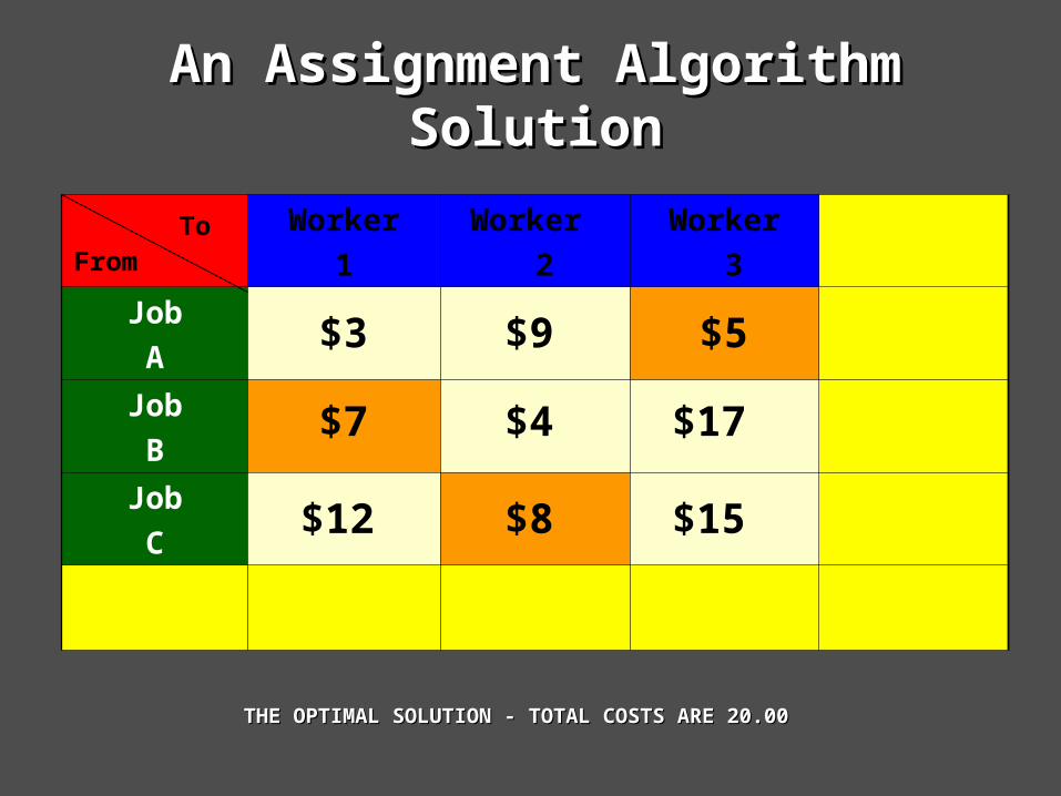
An Assignment Algorithm SolutionAn Assignment Algorithm Solution
Worker
1
Worker
2
Worker
3
Job
A
Job
B
Job
C
$3
$4
$9
$7
$12 $15
$17
$8
$5
FromTo
THE OPTIMAL SOLUTION - TOTAL COSTS ARE 20.00 THE OPTIMAL SOLUTION - TOTAL COSTS ARE 20.00

CharacteristicsCharacteristics
Guarantees an optimal Guarantees an optimal solution since it is a solution since it is a linear programminglinear programming modelmodel

CharacteristicsCharacteristics Also known as the Also known as the Hungarian Method ,Hungarian Method ,
Flood’s Technique , Flood’s Technique , and the and the Reduced Reduced Matrix MethodMatrix Method
NAMED AFTER MERRILL MEEKS FLOOD,
FAMED OPERATIONS RESEARCHERINDUSTRIAL ENGINEERPh.D, Princeton , 1935

CharacteristicsCharacteristics
Determines the most efficientDetermines the most efficient assignment of jobs to workersassignment of jobs to workers and machines or vice-versaand machines or vice-versa
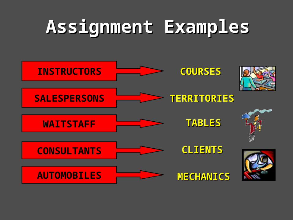
Assignment ExamplesAssignment Examples
COURSESCOURSES
TERRITORIESTERRITORIES
TABLESTABLES
CLIENTSCLIENTS
MECHANICSMECHANICS
SALESPERSONS
WAITSTAFF
CONSULTANTS
AUTOMOBILES
INSTRUCTORS

HISTORYHISTORY
“
Eugene EgervaryEugene Egervary
Denes KonigDenes Konig“
Fundamentalmathematics
developed at the University of
Budapestin 1932
The Assignment Algorithmis also called the
Hungarian Method in their honor

HISTORYHISTORY
Developed in its current form Developed in its current form by Harold Kuhn, PhD by Harold Kuhn, PhD
Princeton, at Bryn Mawr Princeton, at Bryn Mawr College in 1955College in 1955
( 1925 - )( 1925 - )
Model AssumptionsModel Assumptions
Employed only when all workers or machinesEmployed only when all workers or machines are capable of processing all arriving jobsare capable of processing all arriving jobs

Model AssumptionsModel Assumptions
Employed only when all workers or machinesEmployed only when all workers or machines are capable of processing all arriving jobsare capable of processing all arriving jobs
Dictates that only 1 job be assigned to eachDictates that only 1 job be assigned to each worker / machine , and vice-versaworker / machine , and vice-versa
Total number of arriving jobs must equal theTotal number of arriving jobs must equal the total number of available workers / machinestotal number of available workers / machines

Possible Performance CriteriaPossible Performance Criteria
• Profit maximization
• Cost minimization
• Idle time minimization
• Job completion time minimization
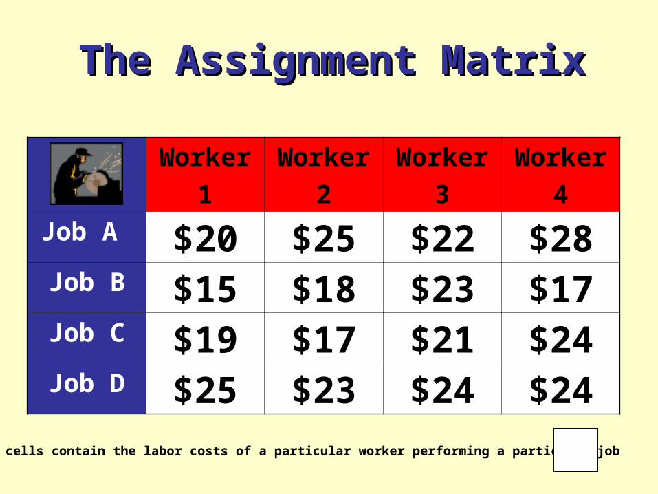
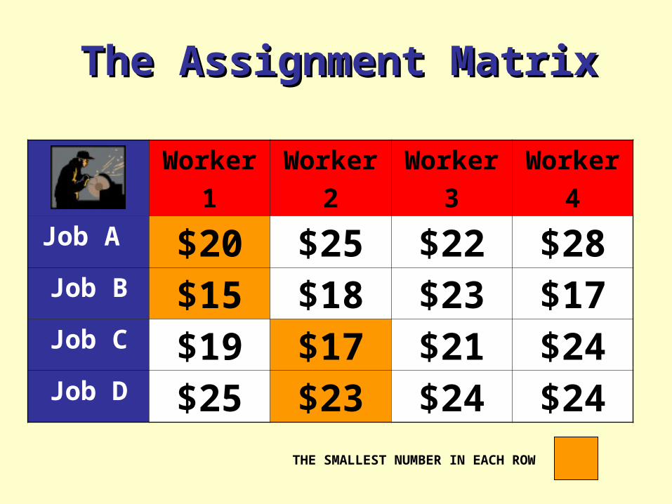
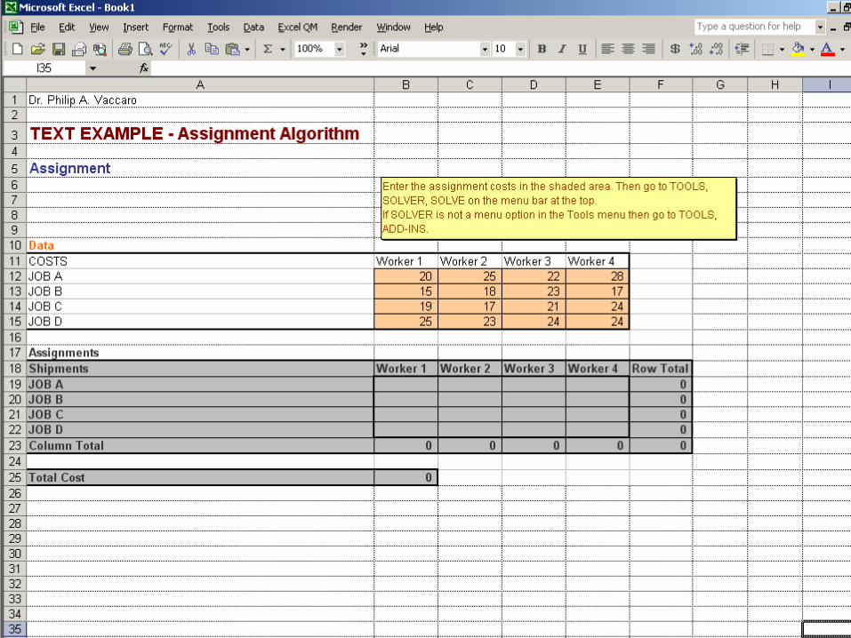
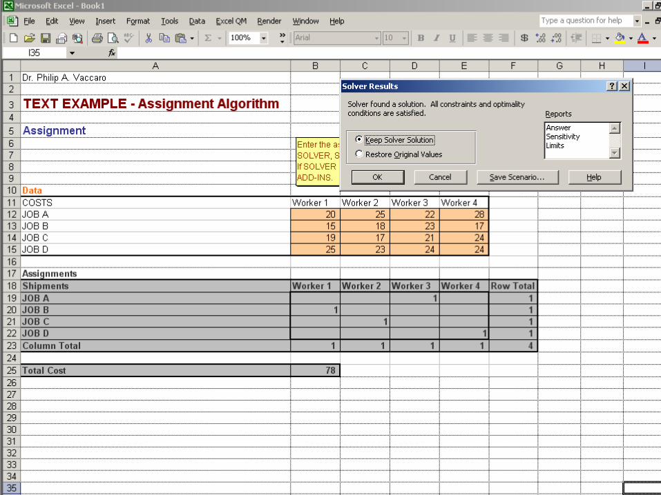
The Assignment MatrixThe Assignment Matrix
Worker
1
Worker
2
Worker
3
Worker
4
Job A $20 $25 $22 $28Job B $15 $18 $23 $17Job C $19 $17 $21 $24Job D $25 $23 $24 $24
These cells contain the labor costs of a particular worker performing a particular job

Assignment Algorithm StepsAssignment Algorithm StepsSTEP ONE - ROWSTEP ONE - ROW REDUCTIONREDUCTION
SUBTRACT THESMALLEST NUMBER IN EACH ROW FROM
ALL THE OTHERNUMBERS IN
THAT ROW
The Assignment MatrixThe Assignment Matrix
Worker
1
Worker
2
Worker
3
Worker
4
Job A $20 $25 $22 $28Job B $15 $18 $23 $17Job C $19 $17 $21 $24Job D $25 $23 $24 $24
THE SMALLEST NUMBER IN EACH ROW

The Assignment MatrixThe Assignment Matrix
Worker
1
Worker
2
Worker
3
Worker
4
Job A $0 $5 $2 $8Job B $0 $3 $8 $2Job C $2 $0 $4 $7Job D $2 $0 $1 $1

The Assignment MatrixThe Assignment Matrix
Worker
1
Worker
2
Worker
3
Worker
4
Job A $0 $5 $2 $8Job B $0 $3 $8 $2Job C $2 $0 $4 $7Job D $2 $0 $1 $1
Assignment Algorithm StepsAssignment Algorithm StepsSTEP TWO - COLUMSTEP TWO - COLUMNN REDUCTIONREDUCTION
SUBTRACT THESMALLEST NUMBER
IN EACH COLUMNFROM ALL THE
OTHER NUMBERS IN THAT COLUMN

The Assignment MatrixThe Assignment Matrix
Worker
1
Worker
2
Worker
3
Worker
4
Job A $0 $5 $2 $8Job B $0 $3 $8 $2Job C $2 $0 $4 $7Job D $2 $0 $1 $1
THE SMALLEST NUMBER IN EACH COLUMN

The Assignment MatrixThe Assignment Matrix
Worker
1
Worker
2
Worker
3
Worker
4
Job A $0 $5 $1 $7Job B $0 $3 $7 $1Job C $2 $0 $3 $6Job D $2 $0 $0 $0
THE SMALLEST NUMBER IN EACH COLUMN

The Assignment MatrixThe Assignment Matrix
Worker
1
Worker
2
Worker
3
Worker
4
Job A $0 $5 $1 $7Job B $0 $3 $7 $1Job C $2 $0 $3 $6Job D $2 $0 $0 $0
ROW AND COLUMN REDUCTION PRODUCE THE REDUCED MATRIX
IT IS ALSO CALLED AN OPPORTUNITY COST MATRIX
Assignment Algorithm StepsAssignment Algorithm StepsSTEP THREE - ATTEMPT STEP THREE - ATTEMPT ALL ASSIGNMENTSALL ASSIGNMENTS
ATTEMPT TO MAKEALL THE REQUIRED
MINIMUM COSTASSIGNMENTS
ONLY THOSECELLS
CONTAINING“ 0 ”
OPPORTUNITYCOSTS ARE
CANDIDATESFOR MINIMUM
COSTASSIGNMENTS

The Assignment MatrixThe Assignment Matrix
Worker
1
Worker
2
Worker
3
Worker
4
Job A 0 5 1 7Job B 0 3 7 1Job C 2 0 3 6Job D 2 0 0 0
THE OPPORTUNITY COST MATRIX
WE CAN NOW DROP THE DOLLAR SIGNS

The Assignment MatrixThe Assignment Matrix
Worker
1
Worker
2
Worker
3
Worker
4
Job A 0 5 1 7Job B 0 3 7 1Job C 2 0 3 6Job D 2 0 0 0
ATTEMPT TO MAKE FOUR MINIMUM COST ASSIGNMENTS
NON-PERMITTED ASSIGNMENT - XX
XX
XX XX

The Assignment MatrixThe Assignment Matrix
Worker
1
Worker
2
Worker
3
Worker
4
Job A 0 5 1 7Job B 0 3 7 1Job C 2 0 3 6Job D 2 0 0 0
JOB “ B “ WAS NOT ABLE TO BE ASSIGNED
NON-PERMITTED ASSIGNMENT - XX
XX
XX XX

Assignment Algorithm StepsAssignment Algorithm StepsSTEP FOUR - EMPLOY THE “STEP FOUR - EMPLOY THE “H”-FACTOR TECHNIQUEH”-FACTOR TECHNIQUE
IF ALL REQUIREDASSIGNMENTSCANNOT BE
MADE, USE THE “H” - FACTORTECHNIQUE
IT CREATESMORE “ 0 “
CELLS, WHICHIN TURN,
INCREASES THECHANCES OFMAKING ALL
THE REQUIREDASSIGNMENTS

The Assignment MatrixThe Assignment Matrix
Worker
1
Worker
2
Worker
3
Worker
4
Job A 0 5 1 7Job B 0 3 7 1Job C 2 0 3 6Job D 2 0 0 0
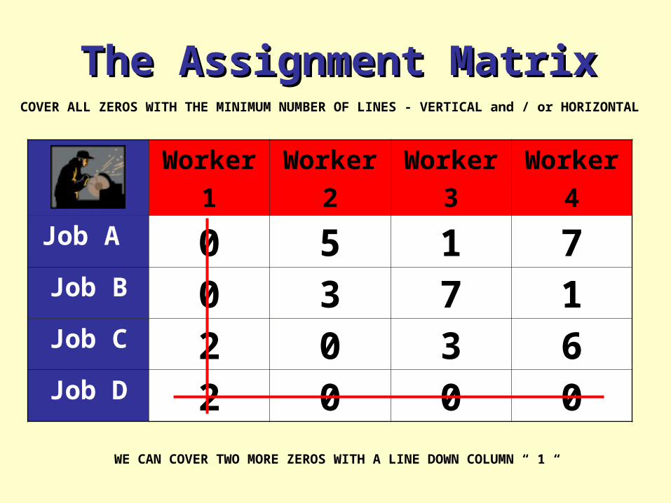
COVER ALL ZEROS WITH THE MINIMUM NUMBER OF LINES - VERTICAL and / or HORIZONTAL
WE CAN COVER THREE ( 3 ) ZEROS WITH A LINE ACROSS ROW “ D “
The Assignment MatrixThe Assignment Matrix
Worker
1
Worker
2
Worker
3
Worker
4
Job A 0 5 1 7Job B 0 3 7 1Job C 2 0 3 6Job D 2 0 0 0
COVER ALL ZEROS WITH THE MINIMUM NUMBER OF LINES - VERTICAL and / or HORIZONTAL
WE CAN COVER TWO MORE ZEROS WITH A LINE DOWN COLUMN “ 1 “

The Assignment MatrixThe Assignment Matrix
Worker
1
Worker
2
Worker
3
Worker
4
Job A 0 5 1 7Job B 0 3 7 1Job C 2 0 3 6Job D 2 0 0 0
COVER ALL ZEROS WITH THE MINIMUM NUMBER OF LINES - VERTICAL and / or HORIZONTAL
WE CAN COVER THE REMAINING ZERO WITH A LINE DOWN COLUMN “ 2 “

The Assignment MatrixThe Assignment Matrix
Worker
1
Worker
2
Worker
3
Worker
4
Job A 0 5 1 7Job B 0 3 7 1Job C 2 0 3 6Job D 2 0 0 0
COVER ALL ZEROS WITH THE MINIMUM NUMBER OF LINES - VERTICAL and / or HORIZONTAL
WE CAN ALTERNATELY COVER THE LAST ZERO WITH A LINE ACROSS ROW “ C “

The Assignment MatrixThe Assignment Matrix
Worker
1
Worker
2
Worker
3
Worker
4
Job A 0 5 1 7Job B 0 3 7 1Job C 2 0 3 6Job D 2 0 0 0
THE “ H “ FACTOR IS THE LOWEST UNCOVERED NUMBER
THE “ H “ FACTOR EQUALS “ 1 “ IN THIS PARTICULAR PROBLEM

The Assignment MatrixThe Assignment Matrix
Worker
1
Worker
2
Worker
3
Worker
4
Job A 0 5 1 7Job B 0 3 7 1Job C 2 0 3 6Job D 2 0 0 0
ADD THE “ H “ FACTOR TO THE CRISS-CROSSED NUMBERS

The Assignment MatrixThe Assignment Matrix
Worker
1
Worker
2
Worker
3
Worker
4
Job A 0 5 1 7Job B 0 3 7 1Job C 3 0 3 6Job D 3 0 0 0
ADD THE “ H “ FACTOR TO THE CRISS-CROSSED NUMBERS

The Assignment MatrixThe Assignment Matrix
Worker
1
Worker
2
Worker
3
Worker
4
Job A 0 5 1 7Job B 0 3 7 1Job C 3 0 3 6Job D 3 0 0 0
SUBTRACT THE “ H “ FACTOR FROM ITSELF AND THE UNCOVERED NUMBERS

The Assignment MatrixThe Assignment Matrix
Worker
1
Worker
2
Worker
3
Worker
4
Job A 0 4 0 6Job B 0 2 6 0Job C 3 0 3 6Job D 3 0 0 0
SUBTRACT THE “ H “ FACTOR FROM ITSELF AND THE UNCOVERED NUMBERS

Assignment Algorithm StepsAssignment Algorithm StepsSTEP FIVE - RE-ATTEMPT ALL STEP FIVE - RE-ATTEMPT ALL REQUIRED ASSIGNMENTSREQUIRED ASSIGNMENTS
RE-ATTEMPT ALLREQUIRED
ASSIGNMENTSAFTER USING
THE “ H “ - FACTORTECHNIQUE
SOMETIMESTHE “ H “FACTOR
TECHNIQUEMUST BE
EMPLOYEDMORE THAN
ONCE, INORDER TO
CREATEENOUGH“ ZERO “CELLSTO DOTHIS
The Assignment MatrixThe Assignment Matrix
Worker
1
Worker
2
Worker
3
Worker
4
Job A 0 4 0 6Job B 0 2 6 0Job C 3 0 3 6Job D 3 0 0 0
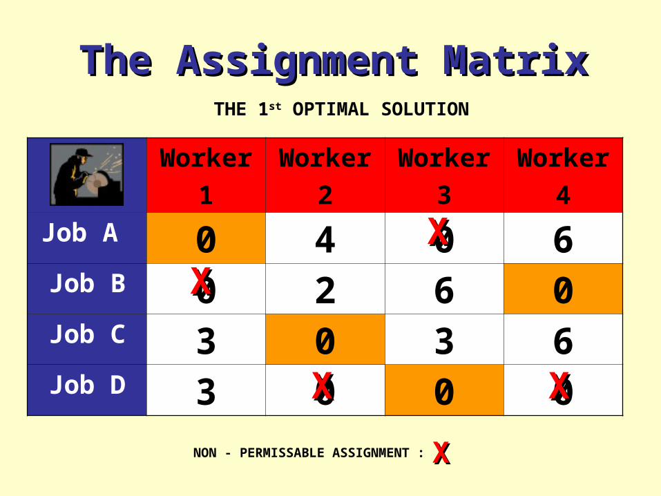
THE 1st OPTIMAL SOLUTION
NON - PERMISSABLE ASSIGNMENT : XX
XXXX
XX XX

The Assignment MatrixThe Assignment Matrix
Worker
1
Worker
2
Worker
3
Worker
4
Job A $20 $25 $22 $28Job B $15 $18 $23 $17Job C $19 $17 $21 $24Job D $25 $23 $24 $24
THE 1st OPTIMAL SOLUTION
TOTAL COST = ( $20. + $17. + $17. + $24 ) = $78.00
The Assignment MatrixThe Assignment Matrix
Worker
1
Worker
2
Worker
3
Worker
4
Job A 0 4 0 6Job B 0 2 6 0Job C 3 0 3 6Job D 3 0 0 0
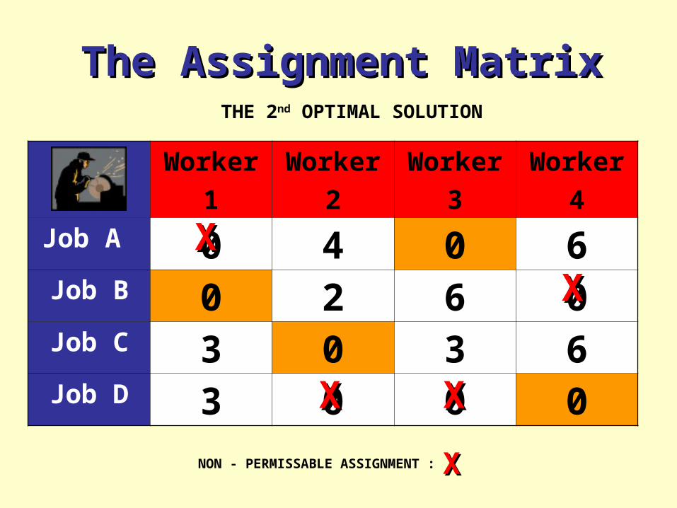
THE 2nd OPTIMAL SOLUTION
NON - PERMISSABLE ASSIGNMENT : XX
XXXX
XX XX
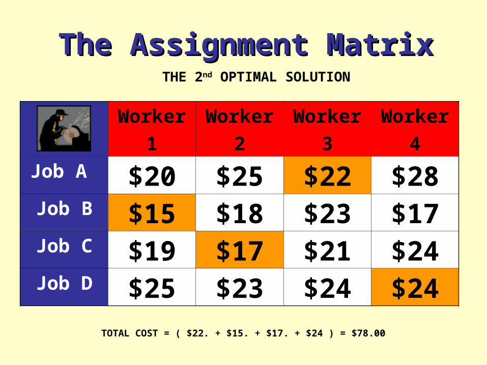
The Assignment MatrixThe Assignment Matrix
Worker
1
Worker
2
Worker
3
Worker
4
Job A $20 $25 $22 $28Job B $15 $18 $23 $17Job C $19 $17 $21 $24Job D $25 $23 $24 $24
THE 2nd OPTIMAL SOLUTION
TOTAL COST = ( $22. + $15. + $17. + $24 ) = $78.00

Alternate Optimal SolutionsAlternate Optimal SolutionsWHY BOTHER ?WHY BOTHER ?

The “The “Alternate Solution”Alternate Solution” Case Case
As a supervisor, you can only recommend a subordinate for a pay raise or promotion.
However, you can give your best workersthe jobs that they really want to do

The Alternate Solution CaseThe Alternate Solution Case
When employed in a shipping environment, alternate routes provide flexibility in the eventof bridge, rail, road closures, accidents, and
other unforeseen events.

Assignment Algorithm withAssignment Algorithm withQMQM forfor WindowsWindows

We Scroll To The
“ ASSIGNMENT “
Module

We Want To Solve ANew Problem

The Dialog Box Appears
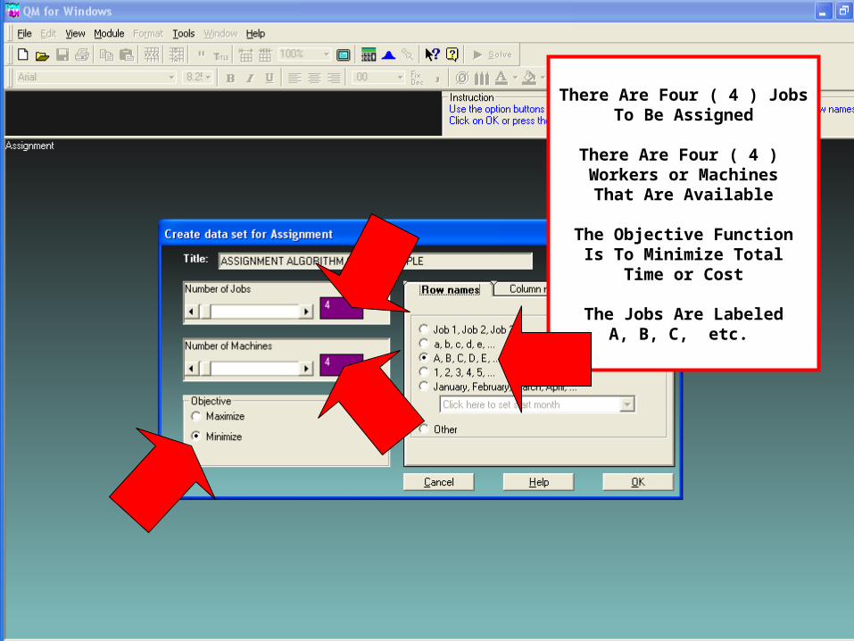
There Are Four ( 4 ) JobsTo Be Assigned
There Are Four ( 4 ) Workers or Machines
That Are Available
The Objective FunctionIs To Minimize Total
Time or Cost
The Jobs Are LabeledA, B, C, etc.
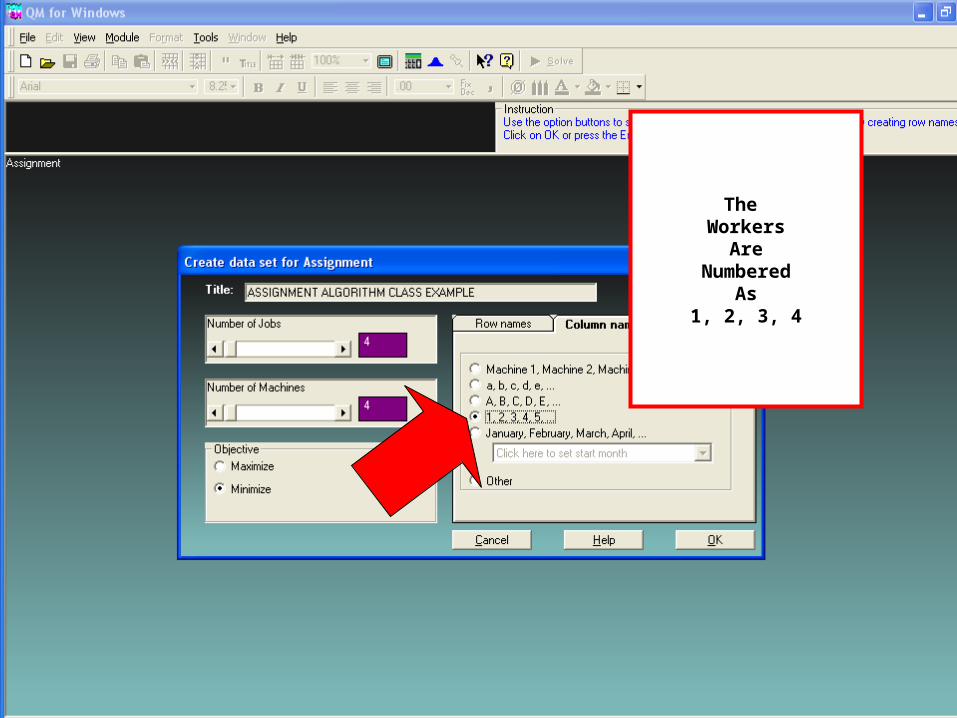
The Workers
AreNumbered
As1, 2, 3, 4
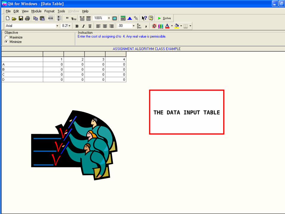
THE DATA INPUT TABLE

THE COMPLETEDDATA INPUT TABLE
INCLUDES THE COST OFPROCESSING EACH JOB
BY EACH WORKER

THE OPTIMAL SOLUTION
Assign Worker 1 to Job AAssign Worker 2 to Job CAssign Worker 3 to Job DAssign Worker 4 to Job B
Total Minimum Cost = $78.00


THE “ TILE “ OPTION
all solution windowscan be displayedsimultaneouslyand removedone by one
after discussion

THE “CASCADE” OPTION
All window solutionscan be discussed
and removedone by oneafterwards

TheAssignmentAlgorithm
Assignment AlgorithmAssignment Algorithm


Templateand
Sample Data


The Assignment Algorithm
Applied Management Science for Decision Making, 1e Applied Management Science for Decision Making, 1e © 2012 Pearson Prentice-Hall, Inc. Philip A. Vaccaro , PhD© 2012 Pearson Prentice-Hall, Inc. Philip A. Vaccaro , PhD
Recommended