Severe air pollution and labor productivity
Teng Li, Haoming Liu, and Alberto Salvo∗
Department of Economics, National University of Singapore
April 10, 2015
Abstract
We examine day-to-day fluctuations in worker-level output over 15 months for apanel of 98 manufacturing workers at a plant located in an industrial city in Hebeiprovince, north China. Long-term workers earn piece-rate wages, with no base payor minimum pay, for homogeneous tasks performed over fixed 8-hour shifts. Overthe sample period, ambient fine-particle (PM2.5) mass concentrations measured atan outdoor air monitor located 2 km from the plant ranged between 10 and 773micrograms per cubic meter (µg/m3, 8-hour means), variation that is an order ofmagnitude larger than what is observed in the rich world today. We document largereductions in productivity, of the order of 15%, over the first 200 µg/m3 rise inPM2.5 concentrations, with the drop leveling off for further increases in fine-particlepollution. A back-of-the-envelope calculation suggests that labor productivity across190 Chinese cities could rise by on average 4% per year were the distributions ofhourly PM2.5 truncated at 25 µg/m3. We also find reduced product quality aspollution rises. Our model allows for selection into work attendance, though we donot find particle pollution to be a meaningful determinant of non-attendance, whichis very low in our labor setting. Subsequent research should verify the externalvalidity of our findings.
Keywords: Air pollution, labor productivity, labor supply, PM2.5, environmental dam-age, benefit-cost analysis
∗Teng Li, Haoming Liu, and Alberto Salvo, Department of Economics, National University of Sin-gapore, 1 Arts Link, Singapore 117570. Email: [email protected], [email protected], [email protected], phone: +65 6516 4876. We thank audiences at the NBER Chinese Economy Meetingand, in particular, Tom Chang, Arik Levinson and Michael Waldman for comments.
1 Introduction
Among the world’s capital cities, Beijing has become notorious for its air pollution.
Between December 2013 and February 2014, the hourly mass concentration of particulate
matter of diameter up to 2.5 microns (PM2.5) in Beijing’s air, as measured at the US
Embassy, averaged 129 micrograms per cubic meter (µg/m3). Several hundred kilometers
away, in an industrial city that is home to workers whom this paper examines, an air
monitor located 2 km from their workplace recorded hourly PM2.5 concentrations that
averaged 221 µg/m3 over the same winter months, that is, over two-thirds higher than
that in Beijing. The maximum reading during our study period, from April 2013 to
June 2014, was reached on December 25, 2013 at 2 pm, namely 919 µg/m3. This severe
level of fine-particle pollution in ambient air is an order of magnitude higher than the
World Health Organization’s guidelines for human exposure sustained over a period of 24
hours—a mean concentration for PM2.5 of no more than 25 µg/m3 is deemed “healthy.”1
While we cannot disclose the name of the city, we note that the city itself and its outskirts
host several large coal-fired power generating units, steel mills, and cement kilns. The
economic geography of the area, in part due to its abundance of coal deposits, as well
as its physical geography, which includes a mountain range on one side, help explain the
state of its air relative to that in more famous Beijing.
China’s severe environmental degradation is the by-product of the nation’s fast
growth in economic activity, and fear of dampening this growth rate is widely regarded
to be one key reason behind its government’s revealed hesitation, to date, in taking swift
action to abate air pollution (Ebenstein et al., 2015). While research on the social bene-
fits of cleaner air has focused on public health, such as longer life expectancy (e.g., Chen
et al., 2013), another potentially large source of gains, labor productivity, has received
considerably less attention in the policy debate. We conjecture that the relative absence
of labor productivity in policy discussions of the damage caused by China’s air owes
1See World Health Organization (2006). The National Ambient Air Quality Standards (NAAQS) setby the United States Environmental Protection Agency establish a PM2.5 “primary standard”—intendedto provide public health protection including the health of vulnerable groups—of 12 µg/m3 over one yearof exposure, and a 24-hour standard of 35 µg/m3. See http://www.epa.gov/air/criteria.html.
1
at least in part to the paucity of rigorous empirical work on this potentially pervasive
manifestation of morbidity.
To the best of our knowledge, only four previous studies have directly addressed the
impact of air pollution on labor supply or productivity while attemping to overcome some
major hurdles that the literature faces. First, people living in areas with higher ambient
air pollution may differ from residents in areas with better air quality, making it difficult
to use cross-sectional data to establish a causal relationship between air quality and labor
productivity. The second challenge is that because most datasets do not record worker-
level output or earnings on a daily basis, one cannot use daily variation in air quality
to examine its effect on worker productivity while flexibly controlling for individual
and seasonal heterogeneity. Nevertheless, the limited existing empirical evidence indeed
suggests that air quality has a significant adverse effect on labor productivity and labor
supply.2
Using a dataset that contains the daily work performance and operating environment
of citrus pickers in southern California in 1973/74, Crocker and Horst (1981) find that
in-sample ozone pollution reduces the productivity of the outdoor workers by up to 2%.
This finding is confirmed by Graff Zivin and Neidell (2012) who use payroll data from a
farm in California’s Central Valley. Graff Zivin and Neidell (GZN hereafter) show that
a 10 ppb (parts per billion) increase in average ozone exposure results in a 4% reduction
in the productivity of workers picking berries and grapes. In their setting, workers are
paid in proportion to their individual output, i.e., on a piece-rate basis, which acts as an
incentive for workers to perform. In a recent working paper, Chang et al. (2014) find that
outdoor air pollution also in California—but now examining fine-particle (PM2.5) rather
than ozone pollution—also affects the indoor work environment. Chang et al. find that
a 10 µg/m3 increase in outdoor PM2.5 concentrations decreases worker productivity by
roughly 6%, while having no significant effect on working hours. One challenge Chang
2Ostro (1983), for example, investigates the relationship between particle pollution (total suspendedparticles, TSP) and labor supply using cross-sectional survey-based data from the 1976 US Health Inter-view Survey. Workers responded to a survey question asking them how many days in the past two weekshad illness or injury prevented them from working. Ostro reports that “a 10% decrease in ambient levelsof TSP is related to a 4.4% decrease in WLD (work loss days).”
2
et al. face is that the indoor work environment they study is naturally ventilated and,
as the authors point out, variation in temperature, if not adequately controlled for, may
confound variation in fine-particle concentrations, which is their main variable of interest.
Finally, Hanna and Oliva (2014) exploit the closure of a large refinery in Mexico City, a
policy that induced exogenous variation in air quality. Examining aggregate data from
an administrative source, and using a difference-in-difference design, Hanna and Oliva
find that the policy-induced reduction in air pollution led to a 4% increase in weekly
working hours for workers living within a 5 km radius of the refinery.
By examining a panel of individual workers at a textile mill located in the province
of Hebei, in northern China, our paper adds to this sparse empirical literature. In
particular, we are able to examine the effect of severe air pollution on labor productivity.
As alluded to in the opening paragraph, the variation in air pollution observed in China
today is much larger than what the extant literature has studied. For instance, daily
mean PM2.5 concentrations range between 2 and 60 µg/m3 in Chang et al. (2014); in our
data, daily means vary between 25 and 687 µg/m3. This large observed variation enables
us to examine the magnitude and the shape of the relationship between particulate
pollution and labor productivity, which can potentially be nonlinear. Knowing whether
there is a nonlinear dose-response will allow policymakers to more accurately estimate
the economic cost of air pollution to which workers in developing countries today, from
China to India to Indonesia, are exposed—levels that are an order of magnitude higher
than in developed countries in North America and Europe. We note that even at ambient
air levels observed in the United States, PM2.5 is understood to be a major source of
health damage, including minor restricted activity (Fann et al., 2012).
We gained access to daily payroll data for 98 machine operators working on parallel
tasks at a common workplace—a department of an industrial plant—during 15 months.
We argue that the labor institution we study coupled with the structure of the data are
ideally suited to the the research question at hand, sharing several features of recent
impactful studies, at lower levels of pollution, in particular, GZN. Like GZN, we are able
to observe labor supply choices and outcomes for the same worker over time, as ambient
3
air pollution fluctuates day in day out, allowing us to control for worker heterogeneity.
Workers are paid on a piece-rate basis for their individual output, which rewards them
for the level of effort that they individually supply (and has the added feature, as GZN
argue, of plausibly containing measurement error in this relatively high-frequency output
variable).3 The piece rate does not vary across workers, consistent with the homogeneity
across tasks and workstations.4 Unlike GZN’s outdoor setting, however, the indoor work
environment we study is temperature controlled and sheltered from rain and wind,5
which we argue enables us to directly control for an important possible confounder of
the effect of pollution on labor productivity. An added benefit of temperature control
at the workplace is that it provides us with an exclusion restriction to identify possible
selection into work attendance, and thus control for selection bias, to the extent that
outdoor temperature—and weather more generally—shifts the probability of showing up
to work, e.g., by changing the value of the outside option such as leisure (Graff Zivin
and Neidell, 2014).
Importantly, while temperature is controlled, indoor air that the workers are exposed
to is not filtered and exchanges with the outdoor environment through one large main
door (leading directly outside and through which yarn and fabric are wheeled in and out,
respectively), as well as through a long array of windows that line one of the sidewalls
(installed over thirty years ago). More generally, an environmental engineering literature
reports tight correlation between outdoor and indoor concentrations for pollutants such
as PM2.5, for typical indoor “microenvironments,” as well as high indoor-outdoor ratios
(see references in Section 2 and in Chang et al. (2014)). Finally, our labor output
data consists of not only quantity produced (meters of fabric) but also the quality of
3To be precise, some of the workers in GZN are paid in proportion to their joint output, which isnot the case in our labor market. Further, in our setting there is no minimum wage or base pay, andworkers are on long-term contracts. Moreover, in contrast to Chang et al. (2014), the work shift in oursetting is of fixed duration, so workers do not choose how many labor hours to supply, conditional onwork attendance, which we model. Otherwise, it is conceivable that a worker might choose the numberof hours worked in part as a function of the level of airborne contaminants, and this choice might bemade jointly with the effort level. We also need not worry that workers might slacken to prolong theirnormal work hours to earn an overtime rate.
4Again for comparison, GZN observe workers picking different crops, with the piece rate varying acrossthe crops. Since the authors pool observations across crops, they need to standardize output units.
5To compare, the pear-packing plant that Chang et al. (2014) study has no temperature control.
4
production (meters of defective fabric), allowing us to examine the effect of air pollution
on the product of labor along this additional margin.
Our main finding is that higher mass concentrations of PM2.5 in outdoor air, as
recorded 2 km from the plant, have a significant adverse impact on contemporaneously
observed worker productivity. While the sign of the estimated impacts is consistent with
what has been found in the small extant literature, the range of variation is larger than
that, to the best of our knowledge, ever examined. Our main result is best described
in Figure 4 below, where the scatter depicts data—mean output per attendant worker
for every date by (8-hour) work shift in the sample—and the lines indicate alternative
non-linear fits.6 Starting at the sample minimum of 10 µg/m3 (8-hour means), every
additional 10 µg/m3 of exposure to PM2.5 over a worker’s shift reduces her total output
by 4.3 meters of fabric, highly significant both statistically and economically, equivalent
to about 0.9% of mean output in the sample (509 m/worker-shift). Estimated marginal
effects are similar up to the 75th percentile of the PM2.5 distribution, at 149 µg/m3, and
halve thereafter (-2.0m of fabric per 10 µg/m3 increase). Beyond the 90th percentile, at
230 µg/m3, the estimated marginal effect is a low and only marginally significant -0.5m
per 10 µg/m3 increase.
In sum, integrating over the first 200 µg/m3 increase in ambient PM2.5 concentra-
tions, from 10 to 210 µg/m3, output falls by 71m, equivalent to 14% of mean output (and
with a standard error of 7m). These are large effects. The non-linearity of the relation-
ship over such wide a range is another result that is new to the literature. We also find
plausible effects of particle pollution on worker attendance which, while statistically sig-
nificant, are economically small; irrespective of its determinants, worker non-attendance
is low in our labor setting. For the subset of our sample for which we observe the quality
of labor product, namely meters of defective fabric produced by worker by shift, we find
that defective output rises with particle pollution.
To better interpret the implications of our findings, including the estimated non-linear
6As we subsequently explain, regression models include fixed effects for year-month, day-of-week,public holidays (that the workplace did not observe), time-of-day and individual worker, among othercontrols, including non-linear functions of co-pollutant concentrations, namely SO2 and CO which, unlikeozone, are emitted from surrounding industry and may also penetrate indoors.
5
relationship over a wide range of particle pollution, we perform a back-of-the-envelope
calculation. We take our estimated worker-day level model and predict aggregate output
produced by the studied labor institution (i.e., the department of 98 individual workers
and their characteristics) were it to be hypothetically transplanted to each of 190 major
cities in mainland China, under currently observed ambient air levels of PM2.5. This
provides a baseline for each Chinese city over the course of 12 (in-sample) months. We
then repeat the exercise, again for each of the 190 cities, predicting output by the modeled
labor institution hypothetically transplanted to the given city, under the counterfactual
scenario that PM2.5 levels in the city were not to exceed 25 µg/m3 at any hour during
the course of the 12 months. Aggregating across the 190 cities and over the different
seasons of the year, a comparison between counterfactual and actual scenarios suggests
that aggregate output would rise by 3.8%. Of course this exercise has several limitations,
not least that it ignores the costs of pollution control given the state of China today, but
it serves to highlight one large and often overlooked benefit of abating air pollution.7
The rest of the paper is structured as follows. Section 2 discusses the labor institution
and the environment workers are exposed to. Section 3 lays out the conceptual framework
and the empirical model of worker choices. Sections 4 and 5 estimate the impact of PM2.5
pollution on worker non-attendance and worker output, respectively. Section 6 presents
implications of our findings and concludes.
2 Data and descriptive analysis
Our data on worker output is made available thanks to a special agreement with man-
agement at a textile operation in a city in the northern province of Hebei, China. We
do not name the city to protect the operation’s confidentiality, as agreed with manage-
ment.8 The operation we examine—namely, the textile department—is part of a larger
industrial complex. The textile department obtains yarn from an upstream operation
7A second back-of-the-envelope calculation in the Appendix considers whether the principal at theworkplace would privately benefit from installing indoor pollution control, as in a semiconductor plant.
8For reference, Hebei province surrounds Beijing. By management, we refer to several employees atthe firm in managerial, administrative or technical positions with whom we have developed a relationship.
6
within the firm and processes the input into fabric rolls, which are then sold to buy-
ers across China and abroad.9 The department runs around the clock, seven days per
week, but shuts down over short multiday periods which typically include or overlap with
public holidays such as the weeks of Chinese New Year and National Day. Our sample
comprises the period between April 1, 2013 and June 30, 2014. During this period there
were 456 days, 54 days of which (12%) the department produced no output. Excluding
these plant holidays, our sample thus consists of 402 dates.
Labor organization. The department operates three shifts of fixed, 8-hour dura-
tion, starting at: (i) 0 am (to 8 am), (ii) 8 am (to 4 pm), and (iii) 4 pm (to 0 am the next
day). Workers are divided into three teams which rotate, as a team, among these shifts
every four workdays. For example, in our sample, in 2013, Team 1 worked the 0 am shift
from April 6 to 9, the 4 pm shift from April 10 to 13, the 8 am shift from April 14 to 17,
and so on. Thus, we observe each worker and her team repeatedly working in each of the
three shifts. This allows us to control for effects that may be specific to the shift, such as
the likelihood that a worker is absent on a given date, or any shift-specific variation in
productivity. As we describe below, we observe each worker’s quantity of output, total
and defective, expressed in meters of fabric, by date (and we know the shift). According
to management, workers typically work the fixed 8-hour shift along with their team, and
do not select the number of hours worked; for this reason, this measure of hours is not
recorded. We return to this institutional feature below.
A shift is staffed by about 30 workers and one supervisor. Each workstation is
operated by one worker, and workstations operate in parallel. Each worker’s workstation
consists of 10 machines, or looms, valued at about US$ 30,000 each. The task being
performed is quite homogeneous across workers and workstations. The job description
is to walk up and down the workstation and attentively observe the looms as they weave
threads into fabric. Typically, 1 to 2 threads will break apart per machine per hour,
9There are two upstream operations within the firm. First, a preparatory department purchasescotton from the nearby provinces of Shandong and Jiangsu and the northwestern province of Xinjiang,which it then cleans and draws. Next, a yarn department spins and passes cotton into yarn. The textiledepartment that we study takes the yarn and weaves threads into fabric. We are unaware of any inputshortages, including electricity, during the sample period. Also, in view of its widespread geographicnature, demand for the operation’s produce is unlikely to depend on local economic activity.
7
requiring skill and effort from the worker to reconnect the thread, a task that might take
several minutes. Therefore, a worker will typically reconnect 10-20 threads across the
10 machines every hour, and in extreme cases this number can rise to 50-60 threads per
hour. Day in, day out, a worker tends to return to the same workstation. There is some,
albeit limited, variation in composition across workstations, in that some workstation’s
machines are programmed to produce fabric of type 133, others produce fabric type 134.
In practice, “standard” output rates vary slightly according to whether machines are
set up to produce fabric type 133 or 134: 510 and 495 meters of fabric per 10-machine
workstation per 8-hour shift, respectively.10 Due to setup costs, machine composition
changes only rarely within workstation.
The machines are fairly new, having been purchased in block when the firm was
privatized in the early 2000s. We do not observe machine breakdowns. Management
informed us that machines, likely because they are only a decade old, break down rarely—
preserving machinery is another reason justifying indoor temperature control in this
firm and the wider industry. In the event that a machine breaks down, the worker’s
variable pay is pro-rated based on her output using the functioning machines. (We
subsequently detail both variable pay and temperature control.) Every batch of 10
machines, comprising a workstation, undergoes planned maintenance every fortnight,
which may include a simple inspection by a maintenance crew member.
While work in the textile department is capital intensive, productivity depends crit-
ically on the quality of its workers. Our understanding is that the quality of labor is a
function of the skill (experience) and attentiveness (effort level) of the worker. The ap-
propriate unit of analysis is the individual worker, as there is minimal complementarity
across workers.
There are three types of employees operating the machines. What we label “depart-
ment” workers form the bulk of our sample. These workers are assigned continuously
to work at the textile department. When we observe a department worker produce zero
output on a given date, other than a plant holiday, our interpretation is that the worker
10The numbers 133 and 134 correspond to the fabric’s warp. The weft in both cases is 72.
8
did not attend work. (We also observe some department workers who, before the sample
period ends, are reassigned to other departments or leave the firm, and others who, after
the sample period begins, join as department workers, including those coming from other
departments within the firm.) In total, our sample includes 98 department workers. The
second type of employee who operates the machines is a “cross-department” worker.
These workers work across departments (e.g., preparatory, yarn, textile), to smoothen
fluctuations in aggregate output brought about by planned and unplanned absences in
the workforce. Our sample includes 12 cross-department workers, and for each of these
workers we observe intermittent (though often adjacent) dates with non-zero output. Fi-
nally, the third type of machine operator is labeled a “substitute” worker. These workers
are also brought in to meet demand and to keep the machines from staying idle. Our
data does not include information on these workers.
We base our analysis on the panel of 98 regular department workers.11 For perspec-
tive, the median worker was born in 1970, is female and Han (race), has nine years of
schooling, was hired by the firm in 1991, and is local to the same city as the firm (ac-
cording to the department of human resources’ records). This median worker is married,
with 1994 being the median year of marriage, and has one child, with 1996 being the
median birth year among first children. Thus, workers tend to be middle aged, long-term
employees, and have older children. The median worker typically lives in the vicinity
of the plant, so commuting costs are low. She is also currently on a five-year contract
with the firm. Throughout the entire sample, we observe 33, 40 and 25 department
workers attached to Teams 1, 2 and 3, respectively. As we show in the Appendix, Team
2 experienced more attrition (and entry) over the sample period: counts of department
workers who are attached to Teams 1, 2 and 3 through the end of the sample, on June
30, 2014, are 27, 28 and 21 respectively.
With worker attention being critical and complementarity across workers being min-
imal, workers are paid by the amount of good-quality fabric they individually produce
in each shift. During the sample period, the piece rate was increased once, from CNY
11Our results are robust to including the intermittent output by cross-department workers.
9
0.07 per meter of (133-equivalent) fabric prior to September 29, 2013 to CNY 0.1 sub-
sequently. (By 133-equivalent meters we mean that any output of 134-type fabric is
multiplied by 510/495 to account for the 3% higher throughput of machines when pro-
ducing 133 relative to 134.) The large increase in the piece rate is one reason why we
control for calendar month fixed effects in the empirical analysis.12 This piece rate does
not vary across workers, consistent with the homogeneity across tasks and workstations
(with the exception of the 133 versus 134-type fabric adjustment explained above). Other
than through benefits such as subsidized housing and health insurance, there is no base
pay and all compensation is variable, again, reflecting the importance of skill and effort
as inputs to the production function, with the worker’s “skin in the game.” Similarly,
there is no minimum wage or threshold level above which variable compensation applies
(as there is, for example, in GZN’s study of pollution in California). At the end of her
shift, a worker marks the point at which her production ended and at which the produc-
tion of her colleague, working the subsequent shift at the same workstation, begins. The
rolls of fabric, once complete, are subsequently inspected for defects and payroll records
are updated. The most common defect is fabric that is short of threads (e.g., warps)
that the worker—or machine—failed to detect. While workers are paid based on the
amount of defect-free production, they do not receive pecuniary punishment for produc-
ing defects. To the best of our knowledge, there are no disputes over what constitutes
defect-free fabric, or how individual-level output is recorded. It is these payroll records
that we gained access to. To provide perspective on how much workers earn, a worker
who produces at the sample median of 506 m in a shift earns (after the pay rise) CNY
51, equivalent to about US$ 9, in that shift.13
The key aspect of the individual level productivity data is its longitudinal structure.
Similar to GZN, we are able to follow the same worker, date-shift by date-shift, which
allows us to control for worker heterogeneity. In addition to the quantity of individual
12Our data indicates that the month in our sample with the highest attrition in the department wasSeptember 2013, with 13 departures alone.
13For a rough conversion into US$, divide CNY by 6. Also for perspective, the HebeiStatistics Bureau reports average annual earnings in the city to be a little over 35,000 CNY(www.hetj.gov.cn/hetj/tjsj/ndsj/101400644755604.html).
10
output produced by each worker (ID) over each shift, we observe worker characteristics,
which we can use to learn more about worker heterogeneity. As we illustrate below,
our source of identification, as in GZN, is the day-to-day covariance between the state
of outdoor air pollution and the individual worker’s productivity, once we control for
seasonality and other potential confounders such as temperature in the workplace.
As in other studies (e.g., GZN), a worker occasionally chooses to not attend work. On
the one hand, planned leaves, like plant holidays, are predetermined, so they are unlikely
to depend on day-to-day variation in environmental quality. On the other hand, a worker
might not attend work due to herself or a family member falling sick, or meteorological
and other shocks raising commuting costs or shifting the value of the outside option, e.g.,
a leisure day spent outdoors. Such unplanned non-attendance may in part depend on the
state of air (e.g., pollution might raise the likelihood of an asthma attack), or unplanned
non-attendance and pollution might be correlated through weather shocks (i.e., these
might directly affect health and air). We therefore model the worker’s selection into
work. We note that while health may drive work attendance, shifts in commuting costs
and the value of leisure driven by weather and/or pollution shocks are unlikely to be
sizable, given the setting: about 90% of workers live in nearby housing subsidized by
the employer, and the employer has much information about the employee. As we show
below, worker non-attendance rates are low, of the order of one day per month (on top
of plant holidays, common to all workers). This includes both planned and unplanned
leaves (we are unable to distinguish between the two).
Worker productivity. To illustrate the importance of worker heterogeneity, for
every one of the 98 department workers in our sample we calculate her mean individual
output per shift worked over the entire sample period. The distribution of mean worker
performance is plotted in panel (a) of Figure 1. The figure shows workers’ total output,
i.e., including any defective fabric. The mode is just over 510 m per worker-shift. The
panel indicates that the most productive workers can sustain a production rate that is
up to 40% higher than that of the least productive workers.
Besides comparing mean performance across workers, panels (b) to (d) of Figure 1
11
compare mean performance across dates, separately for the 0 am, 8 am and 4 pm shifts.
(One can think of shift as the time of day.) To prepare these plots, we compute the mean
output per worker for each of the 402×3 date-shift combinations in our sample. This
day-to-day variation in the average productivity of the workforce is of key importance to
our empirical strategy—our task is to uncover the extent to which this temporal variation
in output is driven by variation in ambient PM2.5 concentrations.
Figure 2 provides the same descriptive statistics as Figure 1 but for defective, rather
than total, output. We note that for one of the three teams of workers, Team 3, daily
records on defective output are missing, so the figure considers only the 33+40=73
workers attached to Teams 1 and 2.14 Somewhat surprisingly, some workers are reported
to produce 0 m of defective fabric during the sample period, whereas others produce as
much as 7 m of defects per shift on average. The variation of defective output is similar
across shifts, with a mode at about 2 m per worker, less than 0.5% of the modal output.
Defective quantity is low presumably because workers reduce the rate of output to prevent
defects from being produced in the first place.
Environment workers are exposed to. The department is located inside a single-
storey factory building. (See the Appendix for further details, including pictures.) Air
exchanges between the outdoor and indoor environments through windows that are in-
stalled at the top of sidewalls, and one main large door which leads directly outside. The
building was built in 1982 and has not gone through any major remodeling. This being
northern China, winter conditions require central heating (Chen et al., 2013). Outdoor
summer temperatures can rise above 35 degrees Celsius, and the indoor microenviron-
ment is also air-conditioned. Indoor ambient air temperatures are recorded but are not
available to us over the sample period. To gain perspective, however, we obtained copies
of records on specific more-recent dates, such as July 14 and 20, 2014. While outdoor
temperatures, which we observe, were in the range of 36 to 41 degrees Celsius, indoor
temperatures were recorded between 25 and 31 degrees Celsius. We thus assume that
workers are exposed to a work environment with reasonably well-functioning tempera-
14To complete the description of missing output records, we do not observe Team 3 worker output inJune 2014. Defective output records are also missing on five specific dates surrounding plant holidays.
12
ture controls (we qualify the statement given the age of the system). This allows us to
directly control for a typical confounder—ambient temperature—encountered in studies
of air pollution on health and labor outcomes (e.g., Crocker and Horst, 1981). According
to management, heating and air-conditioning systems are the norm in this industry and
this part of China, in part because extreme temperatures might damage inputs (e.g.,
machines, yarn, labor) and outputs (fabric).
We have access to outdoor meteorological conditions recorded in the same city as the
plant for every three-hour interval in the sample. Temperatures (three-hourly means)
fell below -10 degrees Celsius on two occasions in February 2014, in the early hours of
the morning. Temperatures exceeded 40 degrees Celsius in summer 2013 and May/June
2014, on 13 dates, typically in the early afternoon hours. The northern province of Hebei
is dry year-round. Between April 2013 and June 2014, 0 mm of precipitation was recorded
on more than nine-tenths of all three-hourly intervals; among the rare non-dry intervals,
the median rate of rainfall is a low 0.15 mm/hour, with rain being less rare in warmer
months than in colder ones. Humidity is significantly lower in January than in July,
namely means of 37% versus 62%, respectively. Snow was recorded only on four dates,
and it was labeled light to moderate. Wind speed, a determinant of ambient air pollutant
concentrations, tends to be higher from April to September (an average of 6.6 miles per
hour) compared with the remaining colder months (6.1 mph). Wind tends to blow more
strongly in the afternoon hours. In terms of wind direction, winter temperatures tend
to fall when wind blows from the north rather than the south. Wind direction is quite
variable within season but the pattern is quite stable over the four seasons of the year.
Wind blowing along the north-south axis is more common than along the east-west one,
likely due in part to the mountain range to the west of the city. Daily means obtained
from a second data source are highly consistent with the higher-frequency dataset. In
sum, patterns in the meteorological data are highly plausible.
We obtain ambient air pollutant concentrations recorded by the Chinese Ministry of
Environmental Protection. Mass concentrations, in µg/m3, for PM2.5, PM10, SO2, CO,
NO2, and O3, were recorded every hour at an outdoor monitoring site located only 1.7
13
km from the plant we analyze. The times series are quite complete, e.g., PM2.5 and CO
measurements are missing or invalid for only 8% and 9%, respectively, of the possible
456×24=10944 hourly observations between April 2013 and June 2014. These missing
values are fairly evenly distributed throughout the sample and do not cluster on specific
dates, i.e., missing values for PM2.5 on eight or more consecutive hours occur only on 24
occasions in the sample (e.g., April 22, 2013, May 18, 2013, etc), suggesting the site is
well maintained. Where hourly observations are missing, we use the mean concentration
for the pollutant at the given date-hour recorded at three other outdoor monitoring
sites located between 3 and 5 km of the plant, also maintained by the Ministry. Air
measurements at the city’s four sites are highly correlated. The correlation coefficients
for hourly PM2.5 concentrations at the closest site relative to that at each of the other
three sites are 0.88, 0.89 and 0.91.
We have inspected the annual, weekly and diurnal cycles for PM2.5 and other pol-
lutant concentrations. Patterns are consistent with measurements elsewhere, even if
for other atmospheric systems, e.g., Davis (2008), Salvo and Geiger (2014). We briefly
describe these patterns here, and include descriptive regressions below, as this informs
one of our subsequent identification strategies, based on instrumental variables. PM2.5
levels tend to be considerably higher in the colder months over the warmer months—as
much as several hundred µg/m3—and slightly higher in the morning hours than in the
afternoon—a few dozen µg/m3. PM2.5 as a proportion of PM10 mass concentrations
range between 0.4 and 0.8, with higher ratios being observed in the winter. SO2 concen-
trations also peak in the winter, rising all the way from late afternoon and through the
night, likely due in part to high-sulfur coal-fired power generation responding to demand
as temperatures drop. CO concentrations show a similar pattern to SO2. Ozone concen-
trations are higher in the warmer months and at 3 pm, when radiation and temperatures
increase, and are inversely correlated with NO2 concentrations, consistent with ozone
chemistry (Madronich, 2014). In terms of weekly cycles, NO2, SO2 and CO concentra-
tions are somewhat lower on Sundays compared with other days of the week, consistent
with, e.g., nitrogen dioxide’s role as a signature of anthropogenic sources (Beirle et al.,
14
2003). In contrast, PM2.5 concentrations exhibit a less pronounced weekly cycle, given
their longer life-time in the atmosphere, consistent with observations elsewhere (Salvo
et al., 2015). In short, we deem the Ministry’s pollution data to be reliable.
We do not observe PM2.5 mass concentrations inside, right by the workstations.
We rely on a literature in environmental sciences, engineering and epidemiology that
finds that fine (including ultrafine) particles penetrate indoors, e.g., Morawska et al.
(2001), Cyrys et al. (2004), Gupta and Cheong (2007). For example, Cyrys et al. (2004)
report, for a given microenvironment they study, that with “closed windows, the I/O
(indoor-outdoor) ratios for PM2.5 are . . . 0.63 . . . (and) that more than 75% of the daily
indoor variation could be explained by the daily outdoor variation for those pollutants.”
The workplace we study is set in a building that is over 30 years old and is directly
linked to a ventilated outdoor environment by way of a long row of closed (though
likely imperfectly sealed) windows and a large open door, through which yarn (input)
and fabric (output) are regularly wheeled in and out. For comparison, Chang et al.
(2014) also proxy for the quality of indoor air using measurements from official outdoor
monitors. With observational data, high-frequency indoor measurements are unlikely to
be available. In studies where indoor air is measured, this is likely on an experimental
basis and may affect behavior; further, measurements (e.g., on handhelds, measuring
particle counts) may be of inferior quality compared to an official monitoring site that
is regularly subject to standard QA/QC procedures (quality assurance/quality control).
It is also conceivable that the worker may arrive to work already feeling unwell due to
her exposure to pollution in the preceding hours, while at home or elsewhere (PM2.5
concentrations tend to be persistent over adjacent hours compared to variation across
multiple days, when, e.g., wind conditions change).15
Table 1 reports sample statistics, consistent with the discussion above, at the worker-
date-shift level (e.g., output), the worker level (demographics), and the date-shift level
(environment). Given the frequency of the worker output data, we compute means of
15A possibility we are considering is to conduct simultaneous PM2.5 measurements, based on 8-hourfilters, or perhaps less conspicuous high-frequency handhelds, at different locations of the indoor andadjacent outdoor environments.
15
hourly pollutant concentrations within each 8-hour (i.e., 402×3) date-shift combination
in the sample. Again, PM2.5 concentrations are those measured at a monitor located
2 km away (and we impute missing hourly observations using available observations
from the three other nearby monitors that same hour), and these tend to exceed those
measured by the US Embassy in Beijing.
The mean PM2.5 mass concentration is 124 µg/m3. Figure 3 plots the kernel density
function of 8-hour mean PM2.5 concentrations across all date-shifts in the sample period,
in panel (a), as well as residuals of mean PM2.5 concentrations when these are regressed
on calendar-month, day-of-week and time-of-day (shift) fixed effects. The wide variation
in ambient fine-particle pollution, even when seasonality is accounted for, as is evident
in panel (b), will enable us to compare the productivity benefits from abating pollution
over the wide range of pollution levels we observe in our sample.16 For comparison, panel
(c) plots the kernel density function of 8-hour mean PM2.5 concentrations measured by
the US Embassy in Beijing, over the same sample period. Relative to levels recorded by
the Ministry 2 km from the plant, concentrations in Beijing several hundred km away
tend to be lower (a mean of 95 against 124 µg/m3 over the study period)—this happens
particularly in the mornings during the colder months.
Observed determinants of fine-particle pollution. Given the central impor-
tance of environmental variables to our study, we now examine the observed determinants
of PM2.5 in ambient air. The purpose is twofold. First, an analysis of the covariance
of PM2.5, season and meteorology serves as a check on the quality of the data. Second,
the analysis provides the first stage to a 2SLS estimator we subsequently report on.
Table 2 regresses mean PM2.5 concentrations recorded at the monitor 2 km away on
time-varying fixed effects and meteorological conditions recorded in the same city. An
observation is a date by shift combination over the sample period April 1 2013 to June 30
2014. PM2.5 concentrations are missing for 5 combinations, thus there are 456×3-5=1363
observations. Column (1) shows the importance of seasonal, weekly and within-day
16For perspective, (24-hour) PM2.5 mass concentrations vary between 2 to 60 µg/m3 in Chang et al.(2014)’s sample, in California. In contrast, (8-hour) PM2.5 levels exceed 60 µg/m3 in about three-quarters of our sample. See the final section on implications.
16
cycles, both anthropogenic and natural. The predictive power of year-month, day-of-
week and time-of-day (i.e., for 8-hour shifts starting at 0 am, 8 am and 4 pm) indicators
is such that the R2 is 38%. (We allow the shift fixed effect to vary by the quarter of
the year, and could do likewise with day of week.) Adding meteorological conditions
in column (2) raises R2 to 45%. PM2.5 concentrations are increasing in temperature
and humidity (maximum and minimum recorded for the date-shift observation). PM2.5
also increases with atmospheric pressure. Relative to zero rain, precipitation averaging
as low as between 0 and 0.5 mm/hour is associated with a reduction of 19 µg/m3 in
PM2.5 levels. A similar downward effect is observed for precipitation in excess of 0.5
mm/hour, which is the case for only 2% of observations. Relative to weak winds, wind
speeds between 5 and 10 miles/hour reduce PM2.5 concentrations by 7 µg/m3; even
stronger winds lower PM2.5 concentrations by 16 µg/m3. The direction of wind also has
systematic effects. Not only are the point estimates intuitively signed—they tend to be
highly statistically significant.
While column (2) restricts meteorological effects to be the same year-round, column
(3) reports that allowing quarterly variation in meteorological effects adds 5 percentage
points to the R2 (estimates are omitted for brevity). Column (4) indicates that lagged
meteorology also determines contemporaneous PM2.5 concentrations. For example, rain
in the preceding 8 hours at mean rates of 0-5 mm/hour and 5+ mm/hour significantly
lowers PM2.5 by 27 and 53 µg/m3, respectively, whereas contemporaneous rain at these
rates has a smaller effect (estimates not shown). Column (5) repeats the specification
shown in column (2) taking PM2.5 concentrations in logs as the dependent variable. For
example, precipitation up to 0.5 mm/hour and wind speeds above 10 mph significantly
lower PM2.5 by 15% and 16%, respectively, relative to no rain and weak winds.
Worker output against fine-particle pollution in the raw data. Figure 4
plots mean worker output per shift against the contemporaneous 8-hour mean PM2.5
concentration measured 2 km from the plant. The top and bottom panels use linear and
logarithmic ordinates, respectively, for PM2.5. Each observation in the scatterplot is a
date-shift pair in the sample, and we average total output (i.e., including any defects)
17
across workers in that date-shift (we return to the fitted lines in Section 5). The rela-
tionship shown in the figure is striking. When fine-particle pollution is very high, mean
output per worker per shift lies at the lower end of the productivity distribution. Output
rarely exceeds the sample mean of 509 m per worker per shift when PM2.5 levels rise
above 250 µg/m3; in particular, shift output per worker exceeds the sample mean only
four times out of the 100 date-shifts with PM2.5 levels above 250 µg/m3. Moreover,
among date-shifts with PM2.5 concentrations below 250 µg/m3 (but still mostly severe),
there is clearly a steep negative relationship between labor productivity and PM2.5.
Figure A.8 in the Appendix shows that the production of defective fabric, while low,
tends to rise with air pollution. For perspective, when PM2.5 levels exceed 250 µg/m3,
the mean quantity of defects per worker lies below the sample mean of 3.8 m only 12
times out of the 100 date-shifts. For date-shifts with PM2.5 levels higher than 500 µg/m3,
defects never fall below 5 m per worker, and for date-shifts with PM2.5 exceeding 600
µg/m3, defects never fall below 10 m.
3 Conceptual framework and empirical model
3.1 Conceptual framework
To fix ideas, consider a worker of ability a who works individually over a fixed shift
of eight hours. During this shift, the worker is exposed to ambient air pollution ΩI
(the superscript denotes the indoor work microenvironment), chooses effort level e, and
produces gross output quantity q, a fraction 0 ≤ ξ ≤ 1 of which comes out free of
defects. The worker incurs an effort cost given by the function c(e,ΩI), which exhibits
the following properties:
∂c(·)∂e
> 0,∂c(·)∂ΩI
≥ 0,∂2c(·)∂e2
≥ 0,∂2c(·)∂e∂ΩI
≥ 0.
These conditions state that the cost of working increases in effort and pollution (strictly
and weakly, respectively), and the positive marginal cost of effort weakly increases in
both effort and pollution. We do not make any assumption on the sign of ∂2c(·)/∂ΩI2.
18
We specify net, or defect-free, output quantity q = qξ = q(e, a) as an increasing and
concave function of the effort level, with production and marginal product increasing
strictly and weakly, respectively, in ability. Formally,17
∂q(·)∂e
> 0,∂2q(·)∂e2
< 0,∂q(·)∂a
> 0,∂2q(·)∂e∂a
≥ 0.
As discussed, the worker is paid a piece rate p per unit of defect-free output, does not
receive pecuniary punishment for producing defects, and there is no daily minimum wage.
The piece rate is invariant to air quality and does not vary across workstations, with
workers performing the same parallel tasks on machines of similar vintage and quality.18
Conditional on coming to work, the worker solves:
arg maxepq(e, a)− c(e,ΩI). (1)
The optimal effort level, e∗ = e(ΩI , a), satisfies:
(p∂q(e, a)
∂e− ∂c(e,ΩI)
∂e
)|e=e∗ = 0. (2)
The first term of first-order condition (2) captures the benefit from marginally exerting
more effort while the second term depicts the marginal cost. The total derivative of (2),
with respect to the cost- and output-shifters ΩI and a, yields:
(p∂2q(e, a)
∂e2− ∂2c(e,ΩI)
∂e2
) ∂e(ΩI ,a)∂ΩI
∂e(ΩI ,a)∂a
′ + −∂2c(e,ΩI)
∂e∂ΩI
p∂2q(e,a)∂e∂a
′ dΩI
da
= 0.
Consider an increase in pollution dΩI > 0 (and fix the worker, da = 0). The worker’s
optimal response to this shift in the environment is to reduce effort, and the magnitude
17Where ξ is not observed, specify the properties of total output, q(e, a), similarly.18Where relevant, we adopt the notation in GZN. For comparison, GZN specify ambient pollution as
impacting the output function, rather than the cost of effort, and they do not model ability. One canextend our model to incorporate the probability of job retention as increasing in the level of output (asGZN do). In our setting most workers have worked for the firm over many years.
19
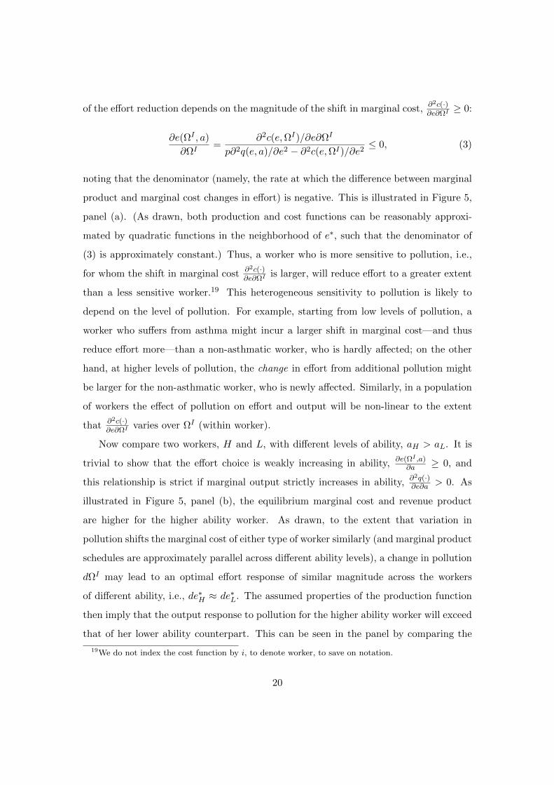
of the effort reduction depends on the magnitude of the shift in marginal cost, ∂2c(·)∂e∂ΩI ≥ 0:
∂e(ΩI , a)
∂ΩI=
∂2c(e,ΩI)/∂e∂ΩI
p∂2q(e, a)/∂e2 − ∂2c(e,ΩI)/∂e2≤ 0, (3)
noting that the denominator (namely, the rate at which the difference between marginal
product and marginal cost changes in effort) is negative. This is illustrated in Figure 5,
panel (a). (As drawn, both production and cost functions can be reasonably approxi-
mated by quadratic functions in the neighborhood of e∗, such that the denominator of
(3) is approximately constant.) Thus, a worker who is more sensitive to pollution, i.e.,
for whom the shift in marginal cost ∂2c(·)∂e∂ΩI is larger, will reduce effort to a greater extent
than a less sensitive worker.19 This heterogeneous sensitivity to pollution is likely to
depend on the level of pollution. For example, starting from low levels of pollution, a
worker who suffers from asthma might incur a larger shift in marginal cost—and thus
reduce effort more—than a non-asthmatic worker, who is hardly affected; on the other
hand, at higher levels of pollution, the change in effort from additional pollution might
be larger for the non-asthmatic worker, who is newly affected. Similarly, in a population
of workers the effect of pollution on effort and output will be non-linear to the extent
that ∂2c(·)∂e∂ΩI varies over ΩI (within worker).
Now compare two workers, H and L, with different levels of ability, aH > aL. It is
trivial to show that the effort choice is weakly increasing in ability, ∂e(ΩI ,a)∂a ≥ 0, and
this relationship is strict if marginal output strictly increases in ability, ∂2q(·)∂e∂a > 0. As
illustrated in Figure 5, panel (b), the equilibrium marginal cost and revenue product
are higher for the higher ability worker. As drawn, to the extent that variation in
pollution shifts the marginal cost of either type of worker similarly (and marginal product
schedules are approximately parallel across different ability levels), a change in pollution
dΩI may lead to an optimal effort response of similar magnitude across the workers
of different ability, i.e., de∗H ≈ de∗L. The assumed properties of the production function
then imply that the output response to pollution for the higher ability worker will exceed
that of her lower ability counterpart. This can be seen in the panel by comparing the
19We do not index the cost function by i, to denote worker, to save on notation.
20
areas of the shaded trapezoids (of similar base). This discussion highlights that worker
ability is another potential source of heterogeneity in the individual response of output
to pollution, as is worker sensitivity in the preceding paragraph.
We can further model the worker’s choice of attending work, with the reservation
utility φ being a possible function of outdoor air pollution ΩO and family composition F .
For example, poor air quality may affect the health of the worker or of a family member
who demands home care from the worker (e.g., Diette et al., 2000), and this demand
for home care is likely to be pronounced for workers with young children. Alternatively,
good air quality may raise the value of outdoor leisure relative to work. As discussed
for the microenvironment we study, fine particles in outdoor air are likely to largely
penetrate the workplace, in which case ΩI and ΩO are highly correlated.
In addition, we posit that meteorological conditions Λ, such as temperature or pre-
cipitation, may drive selection into work attendance, since meteorology may directly
impact own or family health, the relative value of leisure, or the cost of commuting
to work. Importantly, we posit that in our setting meteorology does not affect worker
productivity directly (i.e., conditional on attendance), given that the workplace is tem-
perature controlled and sheltered from rain and wind. This assumption provides an
exclusion restriction to identify an overall selection-plus-productivity effect of pollution.
The exclusion of meteorology from the production and cost functions above—and thus
from the output equation we specify below—in principle allows us to better control for
an otherwise potentially important confounder. Further, given that meteorology shifts
fine particle pollution (per Section 2) but does not affect output directly, we can use
meteorology to instrument for pollution in the output equation, to control for potential
measurement error in PM2.5 or omitted determinants of output.
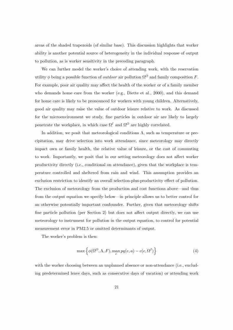
The worker’s problem is then:
maxφ(ΩO,Λ, F ),max
epq(e, a)− c(e,ΩI)
(4)
with the worker choosing between an unplanned absence or non-attendance (i.e., exclud-
ing predetermined leave days, such as consecutive days of vacation) or attending work
21
as planned, and, conditional on attending work, optimizing over the effort level. We
note that features of this labor market, that the work shift is fixed at eight hours and
at a predetermined start time for the worker’s team, imply that we need not model this
additional margin of labor supply.
3.2 Empirical model
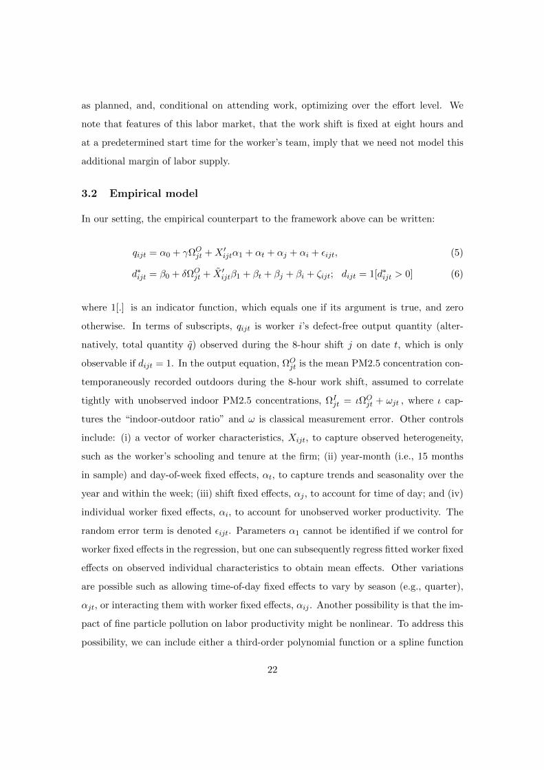
In our setting, the empirical counterpart to the framework above can be written:
qijt = α0 + γΩOjt +X ′ijtα1 + αt + αj + αi + εijt, (5)
d∗ijt = β0 + δΩOjt + X ′ijtβ1 + βt + βj + βi + ζijt; dijt = 1[d∗ijt > 0] (6)
where 1[.] is an indicator function, which equals one if its argument is true, and zero
otherwise. In terms of subscripts, qijt is worker i’s defect-free output quantity (alter-
natively, total quantity q) observed during the 8-hour shift j on date t, which is only
observable if dijt = 1. In the output equation, ΩOjt is the mean PM2.5 concentration con-
temporaneously recorded outdoors during the 8-hour work shift, assumed to correlate
tightly with unobserved indoor PM2.5 concentrations, ΩIjt = ιΩO
jt + ωjt , where ι cap-
tures the “indoor-outdoor ratio” and ω is classical measurement error. Other controls
include: (i) a vector of worker characteristics, Xijt, to capture observed heterogeneity,
such as the worker’s schooling and tenure at the firm; (ii) year-month (i.e., 15 months
in sample) and day-of-week fixed effects, αt, to capture trends and seasonality over the
year and within the week; (iii) shift fixed effects, αj , to account for time of day; and (iv)
individual worker fixed effects, αi, to account for unobserved worker productivity. The
random error term is denoted εijt. Parameters α1 cannot be identified if we control for
worker fixed effects in the regression, but one can subsequently regress fitted worker fixed
effects on observed individual characteristics to obtain mean effects. Other variations
are possible such as allowing time-of-day fixed effects to vary by season (e.g., quarter),
αjt, or interacting them with worker fixed effects, αij . Another possibility is that the im-
pact of fine particle pollution on labor productivity might be nonlinear. To address this
possibility, we can include either a third-order polynomial function or a spline function
22
of PM2.5 concentrations in the regression.
The selection equation contains all the control variables of the output equation (5) in
addition to other variables that affect d∗ijt but not qijt, such as meteorological conditions.
As discussed, meteorology may affect a worker’s reservation utility but, in view of the
temperature controlled work environment, it should not affect workers’ productivity. βi
is an unobserved time invariant worker specific effect that affects a worker’s attendance
decision, and ζijt is a random error term.
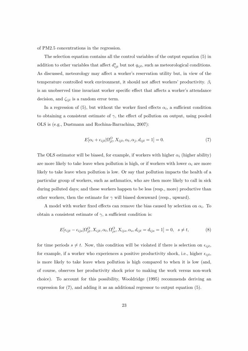
In a regression of (5), but without the worker fixed effects αi, a sufficient condition
to obtaining a consistent estimate of γ, the effect of pollution on output, using pooled
OLS is (e.g., Dustmann and Rochina-Barrachina, 2007):
E[αi + εijt|ΩOjt, Xijt, αt, αj , dijt = 1] = 0. (7)
The OLS estimator will be biased, for example, if workers with higher αi (higher ability)
are more likely to take leave when pollution is high, or if workers with lower αi are more
likely to take leave when pollution is low. Or say that pollution impacts the health of a
particular group of workers, such as asthmatics, who are then more likely to call in sick
during polluted days; and these workers happen to be less (resp., more) productive than
other workers, then the estimate for γ will biased downward (resp., upward).
A model with worker fixed effects can remove the bias caused by selection on αi. To
obtain a consistent estimate of γ, a sufficient condition is:
E[εijt − εijs|ΩOjt, Xijt, αt,Ω
Ojs, Xijs, αs, dijt = dijs = 1] = 0, s 6= t, (8)
for time periods s 6= t. Now, this condition will be violated if there is selection on εijt,
for example, if a worker who experiences a positive productivity shock, i.e., higher εijt,
is more likely to take leave when pollution is high compared to when it is low (and,
of course, observes her productivity shock prior to making the work versus non-work
choice). To account for this possibility, Wooldridge (1995) recommends deriving an
expression for (7), and adding it as an additional regressor to output equation (5).
23
4 The impact of PM2.5 pollution on non-attendance
Whereas plant holidays are predetermined, workers do occasionally choose to not attend
work. Among workers who are in the sample throughout all 15 months, the mean number
of non-attendance days is 15 per worker, i.e., an average of one day per month (on top
of plant holidays, averaging just under 4 days per month). Defining each set of adjacent
days of non-attendance by a worker as a single non-attendance event, or spell, the mean
number of non-attendance spells is only 10 per worker during the 15 months. This
labor market is thus characterized by limited non-attendance. In any case, we seek to
understand its determinants, including the extent to which PM2.5 pollution may drive
non-work decisions, and thus possibly change the composition of the workforce present
each day.
There are a total of 866 worker non-attendance spells in our sample. Of these, 577
lasted for only one day, 161 for two days, and 65 for three days. We exclude the 63 non-
attendance spells that are longer than three days from our analysis, as factors that lead
a worker to take leave for a relatively long period likely differ from those that keep her
from working for only a few days. In particular, longer non-attendance events are likely
to be planned leaves, which are unlikely to be triggered by day-to-day shifts in pollution
(or to correlated with pollution via weather).20 More broadly, when we examine the
relationship between particle pollution and worker output, we can control for the work
choice probability on each date we observe a worker choosing to work.
Table 3 reports estimates for variations of our selection equation, either a linear
probability model (all columns but (3)) or a probit model (column (3)). Across workers,
we have 803 date-shifts of non-attendance (the first day of a non-attendance spell of at
most three days) plus 27,776 date-shifts of work attendance, thus 28,579 observations.
The dependent variable is 1 if the worker chose to start a non-attendance spell and 0 if
she chose to attend work on the given date; the mean value is thus 803/28579=0.028. We
consider the mean PM2.5 mass concentration over the 24 hours that immediately precede
20If we observed which non-attendance events had been agreed in advance, we would not seek toexplain these.
24
the start of a worker’s shift, since the decision to start an (unplanned) non-attendance
spell is likely to occur at this time. We allow for a non-linear relationship by specifying
a linear spline function of PM2.5 concentrations, with three knots set at the first, second
and third quartiles of the PM2.5 distribution, respectively, 62, 94 and 149 µg/m3.21
Column (1) suggests that the impact of (past 24-hour mean) PM2.5 on non-attendance
is highly non-linear in our sample, associated with falling non-attendance as pollution
rises from low levels, i.e., over the first quartile up to 62 µg/m3, while associated with
rising non-attendance when pollution rises above some already severe threshold, over the
fourth quartile beyond 149 µg/m3 (to a maximum of 687 µg/m3 in the sample of 24-hour
means). For example, estimates suggest that as PM2.5 increases from (close to) 0 to 62
µg/m3, a worker is 4 percentage points (0.62×0.063) less likely to choose non-work over
work. Of note, had we controlled for PM2.5 levels linearly, the point estimate would
be small and statistically insignificant. Figure A.9 in the Appendix plots daily rates of
non-attendance against mean PM2.5 concentrations.
In column (2), we control for year-month, day-of-week and time-of-day (0 am, 8 am
or 4 pm shift), as both non-attendance and PM2.5 may follow seasonal/cyclical pat-
terns. Day-of-week includes indicators for any days on the public holiday calendar that
the department was working (see Appendix Table A.1).22 We allow time-of-day effects
to differ across the four quarters of the year. We control for days that immediately
precede or come after plant holidays and find that non-attendance is significantly higher
one day before, and one day after, plant holidays, by 6 percentage points in both cases
(estimates are not reported). To save space, column (2) already includes contemporane-
ous meteorological controls, namely the same ones we included in the PM2.5 regressions
of Table 2 (columns (3) or (4)). The modeling assumption, as per Section 3, is that
meteorological conditions Λ, by changing the attractiveness of outdoor activities or of
21We base the knots, or kink points, on the quartiles of the distribution of 8-hour means, to maintainconsistency throughout. Using quartiles of the distribution of means over the preceding 24 hours wouldyield similar knots, namely, 66, 96 and 146 µg/m3. We sometimes loosely refer to variation from thesample minimum to the 25th percentile as the first (or bottom) quartile, the 25th percentile to themedian as the second quartile, and so on.
22As one might expect, we obtain that non-attendance on such dates is significantly higher (most oftenthe case) or insignificantly different from zero. We do not report for brevity.
25
running outside errands, shift reservation utility φ directly (in addition to indirectly,
as Λ impacts pollution ΩO). Further, meteorology, like pollution, may impact health,
shifting the value of work versus non-work. Adding all of these controls has little impact
on the estimated effect of PM2.5 on non-attendance. We also include a vector of ob-
served worker characteristics. We find that mothers with young children are 2 percentage
points more likely to not attend work, but this is not the case for fathers. Married work-
ers (excluding divorcees and widows) display a higher probability of non-attendance, of
1 percentage point, consistent with a higher reservation utility, whereas local workers
are 2 percentage points less likely to not attend work, perhaps because they enjoy the
support of local family to perform household chores. These findings are consistent with
family composition F shifting reservation utility φ, as we posited in Section 3.
The marginal effects for a probit model, in column (3), are almost identical to the
estimates from the linear probability model of column (2), with common regressors. In
column (4), we replace the worker characteristics of column (2) by a full set of worker
fixed effects, to allow for unobserved heterogeneity. This significantly raises explana-
tory power but again has little impact on PM2.5 estimates. Finally, column (5) tests
robustness in two directions. First, we specify additional flexible meteorological controls
(Auffhammer and Kellogg, 2011), namely: (i) cubic polynomials in the maximum and
minimum temperature, humidity and wind speed, and the maximum precipitation rate,
in the contemporaneous 8-hour shift, allowing these cubic polynomials to vary by time-
of-day; (ii) pairwise interactions for all linear terms in (i); and (iii) linear controls for
the maximum and minimum temperature, humidity and wind speed, and the maximum
precipitation rate, observed in the 24-hour period that precedes the start of the shift.
The second direction in which we test robustness is to control for co-pollutants. Specif-
ically, column (5) also includes linear splines of SO2 and CO concentrations, each with
three knots set at the first, second and third quartiles of the respective distribution.23
The estimated non-linear relationship between PM2.5 and non-attendance thus sur-
vives the inclusion of controls for seasonality, worker, weather, and co-pollutant con-
23The quartiles of the distributions of 8-hour means—which we use throughout—are 37, 56 and89 µg/m3 for SO2 and 1.1, 1.6 and 2.5 µg/m3 for CO.
26
centrations. One possible interpretation of this relationship is as follows. Starting at
relatively low levels, a moderate increase in ambient PM2.5 makes outdoor activities less
attractive, so non-attendance declines with PM2.5 concentration. On the other hand,
once PM2.5 exceeds a high threshold, further increases might affect a worker’s health or
the health of her family, preventing her from working. If PM2.5 drives non-attendance
through its impact on the attractiveness of substitute activities when concentration levels
are relatively low, this impact is likely to vary across seasons as well as across shifts. The
value of activities that compete with work is likely to be higher under mild weather and
during daytime hours. For this reason, Table 4 reports estimates of OLS regressions on
separate samples: (i) by season—“cold,” from October to March, versus “warm,” from
April to September—in columns (1) and (2); and (ii) by shift—again, starting at 0 am,
8 am or 4 pm—in columns (3) to (5).
Reassuringly, estimates suggest that rising PM2.5 is more precisely associated with
lower non-attendance in the warm months, and this effect is more pronounced in the
bottom quartile, up to a concentration of 62 µg/m3, conditions in which outdoor activity
is presumably (still) attractive. During the cold season, or when PM2.5 levels cross into
the second quartile, the coefficient on PM2.5 is imprecisely estimated (and may reverse
sign). We also obtain intuitive estimates on the time-of-day subsample regressions, for
example, rising PM2.5 concentrations in the bottom quartile being more significant,
both statistically and economically, for the 4 pm shift, when the opportunity cost of
work might be higher (e.g., joint family consumption), compared with the 0 am shift.
Column (6) indicates that the negative association between non-attendance and PM2.5,
starting at low levels, is present among mothers with young children, as one might expect
from our possible interpretation.
Another subsample analysis we conduct is for workers with (mean) productivity
above the median of the worker productivity distribution separately from workers below
this median, i.e., high productivity versus low productivity workers (recall panel (a) of
Figure 1). We find that, starting at relatively low levels, rising PM2.5 concentrations
reduce non-attendance more among less productive (lower ability) workers than among
27
their more productive (able) counterparts. We take this result to be consistent with
the simple model we developed in Section 3. While the model suggests that the output
response to increased pollution is larger among workers of higher ability, the gross surplus
from working remains higher for these workers compared to workers of lower ability—
such differing utility can be seen in the area between marginal product and marginal
cost schedules in Figure 5, panel (b). Thus, if the fall in the value of leisure φ(ΩO,Λ, F )
is similar across workers of differing ability, the decline in non-attendance with rising
pollution may be more pronounced among lower ability workers compared to higher
ability ones, as indeed we find.
5 The impact of PM2.5 pollution on output
Table 5 reports OLS estimates for variations of the output equation (5), estimated on
the full sample of 27,776 worker-date pairs between April 2013 and June 2014 for which
a worker attended work.24 The dependent variable is a worker’s total output, in meters,
over an 8-hour work shift; recall the mean is 509 m/shift. Variable definitions are as
in the preceding section, unless noted otherwise. Column (1) specifies a linear spline
of contemporaneously observed 8-hour mean PM2.5 levels. In addition to the knots
specified earlier, corresponding to the first, second and third quartiles of the distribution
of 8-hour means, we specify an additional knot corresponding to the 90th percentile,
namely 230 µg/m3, to allow the estimated impact to vary within the fourth quartile,
where PM2.5 ranges from 149 to a maximum of 773 µg/m3.
Column (2) adds year-month, day-of-week (again, including dummies for any work
days that were on the national holiday calendar), and (quarter-specific) time-of-day fixed
effects, to account for seasonal/cyclical patterns. We also control for: days that imme-
diately precede or come after plant holidays; and a worker’s last day of work prior to
initiating a non-attendance spell, as well as first day of work after returning from one.
Column (3) adds worker characteristics, as in Table 3, column (2). As the workspace is
24Some 8-hour pollution means are missing, so in practice there are slightly fewer observations than27,776. We show below that our findings are robust to taking, as the dependent variable, output net ofdefects, q = qξ, for the subsample of 20,930 worker-dates for which we observe defective output.
28
temperature controlled and sheltered from precipitation and wind, meteorology should
not shift output other than through a possible selection effect or through (as an instru-
ment for) pollution—we consider both channels below and do not, thus, include meteo-
rology, providing an exclusion restriction.25 Relative to column (1), estimated standard
errors in column (2) are lower. Replacing worker characteristics by a full set of worker
fixed effects, in column (4), improves precision further, and the R2 almost triples, from
0.10 to 0.28, yet the estimated non-linear relationship between PM2.5 and worker output
changes only slightly. Similarly, estimated PM2.5 effects hardly change on adding, in
column (5), linear spline functions of contemporaneous SO2 and CO concentrations, and,
in column (6), a selection correction based on the inverse Mills ratio from probit model
(3) in Table 3. We further comment on these specifications below.
Estimates in column (5) suggest that, at the lower fine-particle levels in ambient air,
a 10 µg/m3 increase in (contemporaneous 8-hour mean) PM2.5 concentration reduces
a worker’s output by 4.3 meters of fabric, equivalent to about 0.9% of mean output in
the sample. This is a large effect. Estimated marginal effects are similar or somewhat
lower over the interquartile range of the PM2.5 distribution, up to 149 µg/m3, and then
halve in magnitude (while remaining statistically significant) between the 75th and 90th
percentiles, namely -2.0m of fabric per 10 µg/m3 increase. Beyond the 90th percentile of
the PM2.5 distribution, namely 230 µg/m3, the estimated marginal effect is a low and
marginally significant -0.5m per 10 µg/m3 increase. Figure 4 illustrates the fitted spline,
based on column (5) estimates, as well as the cubic polynomial discussed below.
We can integrate over the first 100 µg/m3 increase in ambient PM2.5 concentrations,
starting at the sample minimum of 10 µg/m3, to obtain a prediction for the output
shortfall over this range, namely 42m of fabric, equivalent to 8.5% of the sample mean,
with estimated standard error (s.e.) of 6m.26 The subsequent 100 µg/m3 increase in
PM2.5, starting at 110 µg/m3, leads to further output loss of 29m (s.e. 3m). In total,
25We check that the estimates on PM2.5 reported in Table 5 are robust to including either set ofmeteorological covariates used in the non-attendance analysis, e.g., in columns (4) and (5) of Table 3.Appendix Figure A.13 plots output against temperature—as well as output against PM2.5 by way ofcontrast—once calendar-month, day-of-week and time-of-day effects have been partialled out.
26For clarity, the point estimate is evaluated as -.43×(62-10)-.41×(94-62)-.43×(110-94). The first100 µg/m3 increase corresponds to a shift from the sample minimum into the third quartile.
29
taking the sample minimum of 10 µg/m3 as the point of departure and raising PM2.5
by 200 µg/m3 leads to an output shortfall of 71m (s.e. 7m), equivalent to 14% of mean
output (or 13% of mean output when PM2.5 levels fall below the 25th percentile).
Returning to the inclusion of individual worker fixed effects in column (4), compared
to observed worker characteristics included in column (3), the increase in explanatory
power is evidence of the role of time-invariant unobservable productivity differences
across workers. However, the finding that PM2.5’s estimated impact on output changes
little when adding this rich set of controls suggests that selection effects driven by un-
observed heterogeneity likely plays a small role in our setting. We note that on adding
time fixed effects in column (2), compared to column (1), the point estimate for the
bottom quartile of the PM2.5 distribution grows more negative. This is consistent with
changes in workforce composition being correlated with pollution, e.g., the workers who
joined the department in the fall, just before the winter when PM2.5 concentrations
tend to be higher, being more productive than those who left in the fall, as we report
in the Appendix. Failing to correct for such a workforce composition effect, in this case
through time fixed effects, would seem to understate the effect of pollution on output.
Columns (4) and (5) thus include a full set of individual fixed effects (respectively,
without and with controls for co-pollutants). We go further and, in column (6), we
control for self-selection following Wooldridge (1995). The variables that are included in
the non-attendance equation but not in the output equation are meteorology variables
and their interactions with quarter. The rationale, as discussed above, is that given the
temperature controlled work environment (and rain and wind), once workers show up
to work their productivity should not depend on contemporaneous meteorology. As we
might expect following the inclusion of worker fixed effects in column (4), the coefficient
on the inverse Mills ratio in column (6) is not statistically significant even at the 10%
level and the estimated impacts are not sensitive to whether we include the inverse Mills
ratio as an additional control.
Table 6 performs a series of subsample analyses, based on the “baseline” specification
in column (5), Table 5. Since the chemical composition, size distribution and thus
30
toxicity of PM2.5—itself a multi-pollutant—may vary across season (Bell, 2012), we
estimate the model separately on two subsamples, “cold” months (again, October to
March) and “warm” (the remainder). Point estimates (columns (1) and (2)) suggest a
larger adverse effect of PM2.5 in the cold months, particularly up to the median of the
PM2.5 distribution. Columns (3) to (5) report estimates when the model is implemented
separately by time of day (shift): while the estimated slopes over the different quartiles
vary across time-of-day subsample, the combined output effect over a 10 to 149 µg/m3
increase in PM2.5 is similar, namely -59m, -56m and -56m for the 0 am, 8 am and 4 pm
shifts, respectively. Our model predicted that the negative impact of PM2.5 on output is
likely to be stronger for higher ability workers compared to those of less ability. This is
supported by the empirical results in columns (6) and (7). Except for days when PM2.5
is at the bottom quartile, an increase in PM2.5 tends to have a more negative impact
on workers with mean productivity above the sample mean.
Sensitivity analysis. We provide some robustness checks in Table 7.27 First, in
column (1), we take as dependent variable the quantity of output net of defects for
the subsample of worker-dates for which we observe defective output (recall records on
defects were not available for Team 3). Second, in column (2), we drop observations
for which a worker’s output during an 8-hour shift might appear either too high or
too low. Specifically, we drop observations with output above the 95th or below the 5th
percentiles, 660 m and 365 m respectively.28 Point estimates, while still highly significant
both economically and statistically, shrink somewhat relative to baseline estimates.
Column (3) replaces the spline function of our baseline specification by a cubic func-
27Among other robustness tests that we do not report here, we add a spline function of mean PM2.5levels over the 24 hours that immediately precede each work shift, on top of contemporaneous PM2.5,to the baseline specification. All contemporaneous and lagged point estimates are negative and mostare highly statistically significant. Specifically, for the bottom quartile the estimated contemporaneouseffect falls slightly from, -43 to -37 (s.e. 12), and the lagged effect is -9 (s.e. 13). For the second quartilethe contemporaneous effect falls more, from -41 to -25 (s.e. 11) and the lagged effect is -46 (s.e. 11).One may speculate from such results whether higher levels of PM2.5 might have a more lasting effectcompared to lower levels. PM2.5 estimates are plotted in Appendix Figure A.14, panel (b).
28See Appendix Figure A.14, panel (a). Our working hypothesis for a few observations with outputabove the nominal capacity of a workstation, as discussed in the Appendix, is that the worker obtainedapproval to continue working into the subsequent shift, noting that such extended hours are presumablyunusual and are not recorded. Our working hypothesis for some low output rates is that the worker feltsick during the shift and went home, or was asked to perform an alternative task.
31
tion in PM2.5 concentrations. For comparability, the fitted cubic is plotted in Figure 4
alongside the estimated spline from column (5), Table 5. Finally, in column (4), Table 7
the cubic specification is estimated by two-stage least squares, using meteorology as an
instrument for PM2.5 pollution. Rather than rely on the entire variation in PM2.5 con-
centrations, the first stage projects PM2.5 on the set of meteorology by quarter controls
(and included exogenous variables). The identifying assumption is that meteorology af-
fects worker output in the climate controlled work environment only through its effect on
PM2.5 pollution (Table 2). The objective is to gauge the extent to which measurement
error in pollution or unobserved determinants of output that correlate with pollution
may be affecting our estimates. Estimates by 2SLS are similar to those by OLS, as can
be seen comparing columns (4) against (3), as well as in Figure 4.
6 Implications and concluding remarks
We take our estimated output model, namely the estimates reported in column (5)
of Table 5, and conduct a back-of-the-envelope calculation, with a view to drawing
implications from these results. We focus on output effects, rather than the combined
attendance-output model, as we are less confident that attendance choices at our specific
labor institution, i.e., the department of 98 individual workers and their characteristics,
generalize to other labor settings; also, we do not attempt here to value activities that
may substitute for work as air pollution varies.29
We predict each of the 98 individual workers’ output over the course of one year (to
capture all seasons) were PM2.5 pollution to follow the time path observed in each of 190
major cities in China today. (See the Appendix for data sources and calculation details.)
Label this baseline scenario “actual pollution.” We then truncate values in these actual
190 city-specific hourly PM2.5 series at 25 µg/m3, and again predict output over the 12
months under this “counterfactual pollution” scenario. For example, the actual PM2.5
level in Guangzhou at 2 pm on October 1, 2013 was 49 µg/m3, and we take it to be
29Were we to predict work attendance across China, we would also need meteorology data (besides airpollution, explained below).
32
min(25, 49) = 25 µg/m3 in the counterfactual. By comparing output predicted under
the two scenarios, and using GDP to aggregate across space and seasons, we obtain a
rough measure of the labor productivity gains that China could experience were PM2.5
pollution to be abated to a concentration no greater than 25 µg/m3 at any point in time
and in space—without, of course, considering abatement costs (or other benefits such
as health), and assuming that other workplaces in China were similar, in terms of dose-
response, to the one we study.30 Table 8 presents estimates of output gains by region
of China and by season. Across the nation and over the year, the predicted output gain
amounts to 3.8%. The largest proportionate output effect, +7.2%, is predicted for North
China (which hosts both the sampled city and Beijing) in the coldest quarter of the year;
the lowest predicted effects correspond to the mild months of July to September. Crudely
multiplying the aggregate output effect by an annual GDP for China of US$ 16.1 trillion
(2013, purchasing-power parity, per the IMF) as well as a labor share of GDP of 40%
(Karabarbounis and Neiman, 2014), yields US$ 240 billion.
We end by comparing the marginal effect found in Chang et al. (2014)—a 6%
drop in indoor worker productivity for every 10 µg/m3 increase in outdoor PM2.5
concentrations—to what we find if we restrict our sample to the same range of mass
concentrations, namely up to 60 µg/m3. We re-estimate our baseline specification on
the sub-sample of observations in which 8-hour mean PM2.5 levels lie below this thresh-
old. This drops 78% of our sample, but we can still count on 6178 observations. (We
also restrict the effect of PM2.5 to be linear, given the reduced range of variation.) We
find that every 10 µg/m3 increase in PM2.5 levels is associated with a 4.6 m output
loss, significant at the 1% level and equivalent to a 0.9% drop relative to mean output
in this sub-sample. That we find highly significant effects of PM2.5 pollution on labor
productivity over a very wide range, yet only one-sixth the magnitude found in Chang
et al. (2014) for a comparatively narrow range, suggests that examining further labor
settings is an important direction for future research.
30For example, the exercise assumes the following to be “similar”: office and farm labor, the natureof manufacturing tasks, outdoor versus indoor exposure to ambient air, the distribution of worker char-acteristics such as age, health and unobserved heterogeneity, the chemical and physical composition ofPM2.5 (a multi-pollutant), and so on.
33
References
Auffhammer, M. and Kellogg, R. (2011). Clearing the air? The effects of gasoline content
regulation on air quality. American Economic Review, 101(6):2687–2722.
Beirle, S., Platt, U., Wenig, M., and Wagner, T. (2003). Weekly cycle of NO2 by GOME
measurements: A signature of anthropogenic sources. Atmospheric Chemistry and
Physics, 3(6):2225–2232.
Bell, M. (2012). Assessment of the health impacts of particulate matter characteristics.
Technical Report 161, Health Effects Institute.
Chang, T., Graff Zivin, J. S., Gross, T., and Neidell, M. J. (2014). Particulate pollution
and the productivity of pear packers. Working Paper 19944, National Bureau of
Economic Research.
Chen, Y., Ebenstein, A., Greenstone, M., and Li, H. (2013). Evidence on the impact of
sustained exposure to air pollution on life expectancy from China’s Huai River policy.
Proceedings of the National Academy of Sciences, 110(32):12936–12941.
Christiani, D. C., Ye, T.-t., Zhang, S., Wegman, D. H., Eisen, E. A., Ryan, L. A.,
Olenchock, S. A., Pothier, L., and Dai, H.-l. (1999). Cotton dust and endotoxin
exposure and long-term decline in lung function: Results of a longitudinal study.
American Journal of Industrial Medicine, 35(4):321–331.
Crocker, T. D. and Horst, R. L., J. (1981). Hours of work, labor productivity, and
environmental conditions: A case study. The Review of Economics and Statistics,
63(3):361–368.
Cyrys, J., Pitz, M., Bischof, W., Wichmann, H.-E., and Heinrich, J. (2004). Relationship
between indoor and outdoor levels of fine particle mass, particle number concentrations
and black smoke under different ventilation conditions. Journal of Exposure Science
and Environmental Epidemiology, 14(4):275–283.
34
Davis, L. W. (2008). The effect of driving restrictions on air quality in Mexico City.
Journal of Political Economy, 116(1):38–81.
Diette, G. B., Markson, L., Skinner, E. A., Nguyen, T. T., Algatt-Bergstrom, P., and Wu,
A. W. (2000). Nocturnal asthma in children affects school attendance, school perfor-
mance, and parents’ work attendance. Archives of Pediatrics & Adolescent Medicine,
154(9):923–928.
Dustmann, C. and Rochina-Barrachina, M. E. (2007). Selection correction in panel data
models: An application to the estimation of females’ wage equations. The Economet-
rics Journal, 10(2):263–293.
Ebenstein, A., Fan, M., Greenstone, M., He, G., and Zhou, M. (2015). Growth, pollution,
and life expectancy: China from 1991-2012. American Economic Review Papers &
Proceedings, (forthcoming).
Fann, N., Lamson, A. D., Anenberg, S. C., Wesson, K., Risley, D., and Hubbell, B. J.
(2012). Estimating the national public health burden associated with exposure to
ambient PM2.5 and ozone. Risk Analysis, 32(1):81–95.
Graff Zivin, J. and Neidell, M. (2012). The impact of pollution on worker productivity.
American Economic Review, 102(7):3652–73.
Graff Zivin, J. and Neidell, M. (2014). Temperature and the allocation of time: Impli-
cations for climate change. Journal of Labor Economics, 321:1–26.
Gupta, A. and Cheong, K. (2007). Physical characterization of particulate matter and
ambient meteorological parameters at different indoor–outdoor locations in Singapore.
Building and Environment, 42(1):237–245.
Hanna, R. and Oliva, P. (2014). The effect of pollution on labor supply: Evidence from
a natural experiment in Mexico City. Journal of Public Economics, (forthcoming).
Karabarbounis, L. and Neiman, B. (2014). The global decline of the labor share. Quar-
terly Journal of Economics, 129(1):61–103.
35
Madronich, S. (2014). Atmospheric chemistry: Ethanol and ozone. Nature Geoscience,
7(6):395–397.
Morawska, L., He, C., Hitchins, J., Gilbert, D., and Parappukkaran, S. (2001). The rela-
tionship between indoor and outdoor airborne particles in the residential environment.
Atmospheric Environment, 35(20):3463–3473.
Ostro, B. D. (1983). The effects of air pollution on work loss and morbidity. Journal of
Environmental Economics and Management, 10(4):371–382.
Salvo, A. and Geiger, F. M. (2014). Reduction in local ozone levels in urban Sao Paulo
due to a shift from ethanol to gasoline use. Nature Geoscience, 7(6):450–458.
Salvo, A., Geiger, F. M., Brito, J., and Artaxo, P. (2015). Fine and ultra-fine particles
and shifting gasoline and ethanol use in urban Sao Paulo. Mimeo.
Wooldridge, J. M. (1995). Selection corrections for panel data models under conditional
mean independence assumptions. Journal of Econometrics, 68(1):115–132.
World Health Organization (1999). Hazard prevention and control in the work envi-
ronment: Airborne dust. Technical Report WHO/SDE/OEH/99.14, World Health
Organization.
World Health Organization (2006). WHO air quality guidelines for particulate matter,
ozone, nitrogen dioxide and sulfur dioxide: Global update 2005. Technical Report
WHO/SDE/PHE/OEH/06.02, World Health Organization.
36
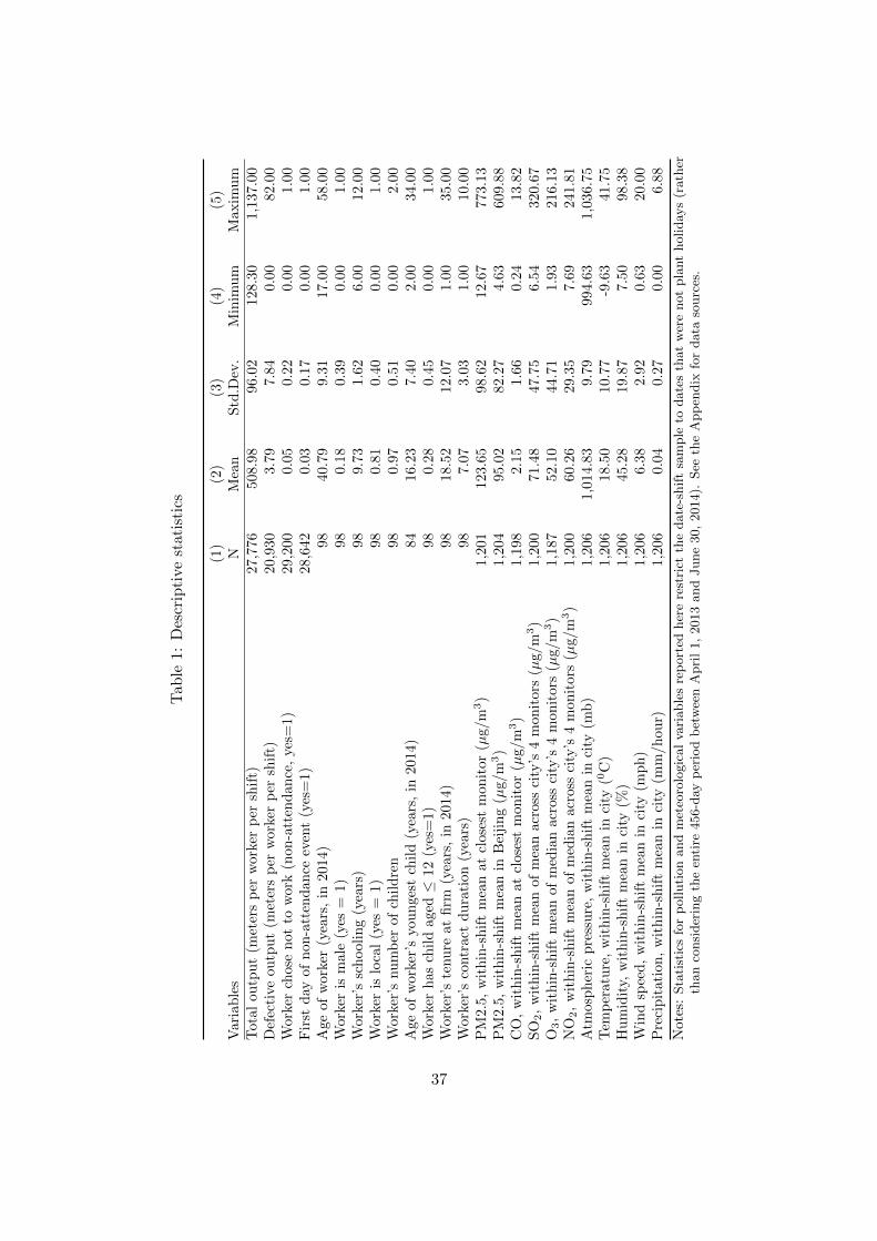
Tab
le1:
Des
crip
tive
stat
isti
cs
(1)
(2)
(3)
(4)
(5)
Var
iab
les
NM
ean
Std
.Dev
.M
inim
um
Maxim
um
Tot
alou
tpu
t(m
eter
sp
erw
orke
rp
ersh
ift)
27,7
76
508.9
896.0
2128.3
01,1
37.0
0D
efec
tive
outp
ut
(met
ers
per
wor
ker
per
shif
t)20,9
30
3.7
97.8
40.0
082.0
0W
orke
rch
ose
not
tow
ork
(non
-att
end
ance
,ye
s=1)
29,2
00
0.0
50.2
20.0
01.0
0F
irst
day
ofn
on-a
tten
dan
ceev
ent
(yes
=1)
28,6
42
0.0
30.1
70.0
01.0
0A
geof
wor
ker
(yea
rs,
in20
14)
98
40.7
99.3
117.0
058.0
0W
orke
ris
mal
e(y
es=
1)98
0.1
80.3
90.0
01.0
0W
orke
r’s
sch
ool
ing
(yea
rs)
98
9.7
31.6
26.0
012.0
0W
orke
ris
loca
l(y
es=
1)98
0.8
10.4
00.0
01.0
0W
orke
r’s
nu
mb
erof
chil
dre
n98
0.9
70.5
10.0
02.0
0A
geof
wor
ker’
syou
nge
stch
ild
(yea
rs,
in20
14)
84
16.2
37.4
02.0
034.0
0W
orke
rh
asch
ild
aged≤
12(y
es=
1)98
0.2
80.4
50.0
01.0
0W
orke
r’s
tenu
reat
firm
(yea
rs,
in20
14)
98
18.5
212.0
71.0
035.0
0W
orke
r’s
contr
act
du
rati
on(y
ears
)98
7.0
73.0
31.0
010.0
0P
M2.
5,w
ith
in-s
hif
tm
ean
atcl
oses
tm
onit
or(µ
g/m
3)
1,2
01
123.6
598.6
212.6
7773.1
3P
M2.
5,w
ith
in-s
hif
tm
ean
inB
eiji
ng
(µg/
m3)
1,2
04
95.0
282.2
74.6
3609.8
8C
O,
wit
hin
-sh
ift
mea
nat
clos
est
mon
itor
(µg/
m3)
1,1
98
2.1
51.6
60.2
413.8
2S
O2,
wit
hin
-sh
ift
mea
nof
mea
nac
ross
city
’s4
mon
itors
(µg/m
3)
1,2
00
71.4
847.7
56.5
4320.6
7O
3,
wit
hin
-sh
ift
mea
nof
med
ian
acro
ssci
ty’s
4m
on
itors
(µg/m
3)
1,1
87
52.1
044.7
11.9
3216.1
3N
O2,
wit
hin
-sh
ift
mea
nof
med
ian
acro
ssci
ty’s
4m
on
itors
(µg/m
3)
1,2
00
60.2
629.3
57.6
9241.8
1A
tmos
ph
eric
pre
ssu
re,
wit
hin
-sh
ift
mea
nin
city
(mb
)1,2
06
1,0
14.8
39.7
9994.6
31,0
36.7
5T
emp
erat
ure
,w
ith
in-s
hif
tm
ean
inci
ty(0
C)
1,2
06
18.5
010.7
7-9
.63
41.7
5H
um
idit
y,w
ith
in-s
hif
tm
ean
inci
ty(%
)1,2
06
45.2
819.8
77.5
098.3
8W
ind
spee
d,
wit
hin
-sh
ift
mea
nin
city
(mp
h)
1,2
06
6.3
82.9
20.6
320.0
0P
reci
pit
atio
n,
wit
hin
-sh
ift
mea
nin
city
(mm
/hou
r)1,2
06
0.0
40.2
70.0
06.8
8
Not
es:
Sta
tist
ics
for
polluti
on
and
met
eoro
logic
al
vari
able
sre
port
edher
ere
stri
ctth
edate
-shif
tsa
mple
todate
sth
at
wer
enot
pla
nt
holiday
s(r
ath
erth
an
consi
der
ing
the
enti
re456-d
ayp
erio
db
etw
een
Apri
l1,
2013
and
June
30,
2014).
See
the
App
endix
for
data
sourc
es.
37
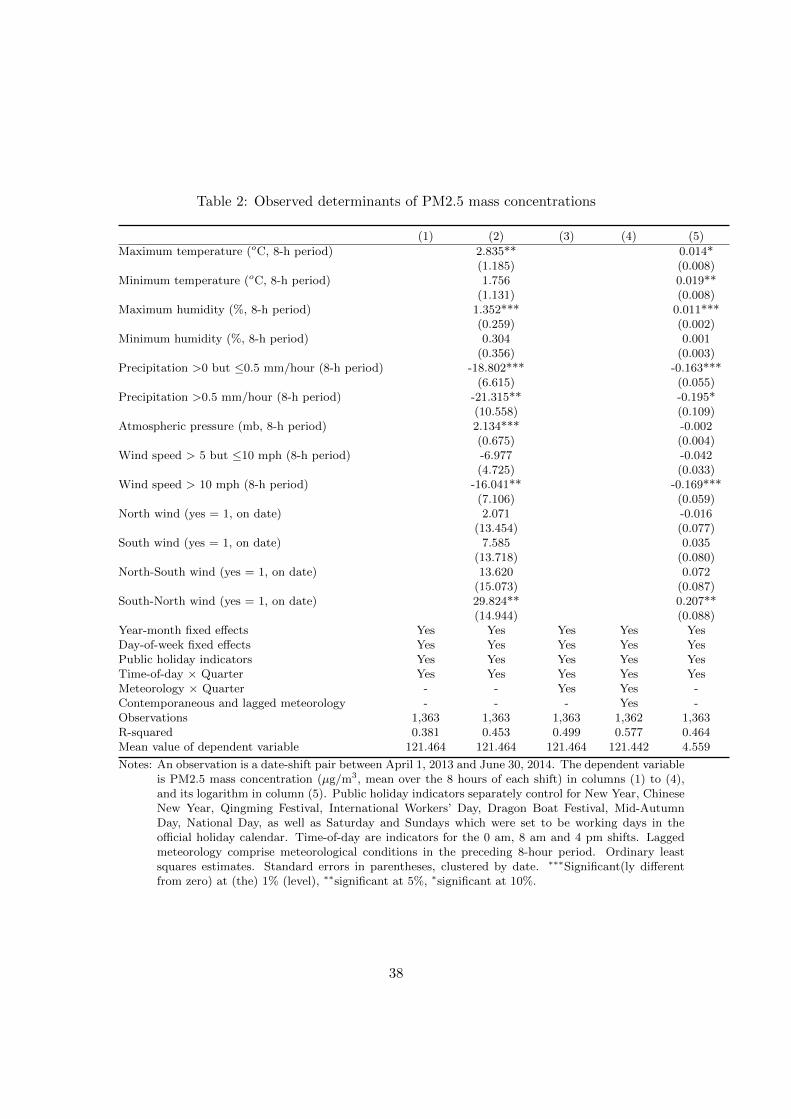
Table 2: Observed determinants of PM2.5 mass concentrations
(1) (2) (3) (4) (5)
Maximum temperature (oC, 8-h period) 2.835** 0.014*(1.185) (0.008)
Minimum temperature (oC, 8-h period) 1.756 0.019**(1.131) (0.008)
Maximum humidity (%, 8-h period) 1.352*** 0.011***(0.259) (0.002)
Minimum humidity (%, 8-h period) 0.304 0.001(0.356) (0.003)
Precipitation >0 but ≤0.5 mm/hour (8-h period) -18.802*** -0.163***(6.615) (0.055)
Precipitation >0.5 mm/hour (8-h period) -21.315** -0.195*(10.558) (0.109)
Atmospheric pressure (mb, 8-h period) 2.134*** -0.002(0.675) (0.004)
Wind speed > 5 but ≤10 mph (8-h period) -6.977 -0.042(4.725) (0.033)
Wind speed > 10 mph (8-h period) -16.041** -0.169***(7.106) (0.059)
North wind (yes = 1, on date) 2.071 -0.016(13.454) (0.077)
South wind (yes = 1, on date) 7.585 0.035(13.718) (0.080)
North-South wind (yes = 1, on date) 13.620 0.072(15.073) (0.087)
South-North wind (yes = 1, on date) 29.824** 0.207**(14.944) (0.088)
Year-month fixed effects Yes Yes Yes Yes YesDay-of-week fixed effects Yes Yes Yes Yes YesPublic holiday indicators Yes Yes Yes Yes YesTime-of-day × Quarter Yes Yes Yes Yes YesMeteorology × Quarter - - Yes Yes -Contemporaneous and lagged meteorology - - - Yes -Observations 1,363 1,363 1,363 1,362 1,363R-squared 0.381 0.453 0.499 0.577 0.464Mean value of dependent variable 121.464 121.464 121.464 121.442 4.559
Notes: An observation is a date-shift pair between April 1, 2013 and June 30, 2014. The dependent variableis PM2.5 mass concentration (µg/m3, mean over the 8 hours of each shift) in columns (1) to (4),and its logarithm in column (5). Public holiday indicators separately control for New Year, ChineseNew Year, Qingming Festival, International Workers’ Day, Dragon Boat Festival, Mid-AutumnDay, National Day, as well as Saturday and Sundays which were set to be working days in theofficial holiday calendar. Time-of-day are indicators for the 0 am, 8 am and 4 pm shifts. Laggedmeteorology comprise meteorological conditions in the preceding 8-hour period. Ordinary leastsquares estimates. Standard errors in parentheses, clustered by date. ∗∗∗Significant(ly differentfrom zero) at (the) 1% (level), ∗∗significant at 5%, ∗significant at 10%.
38
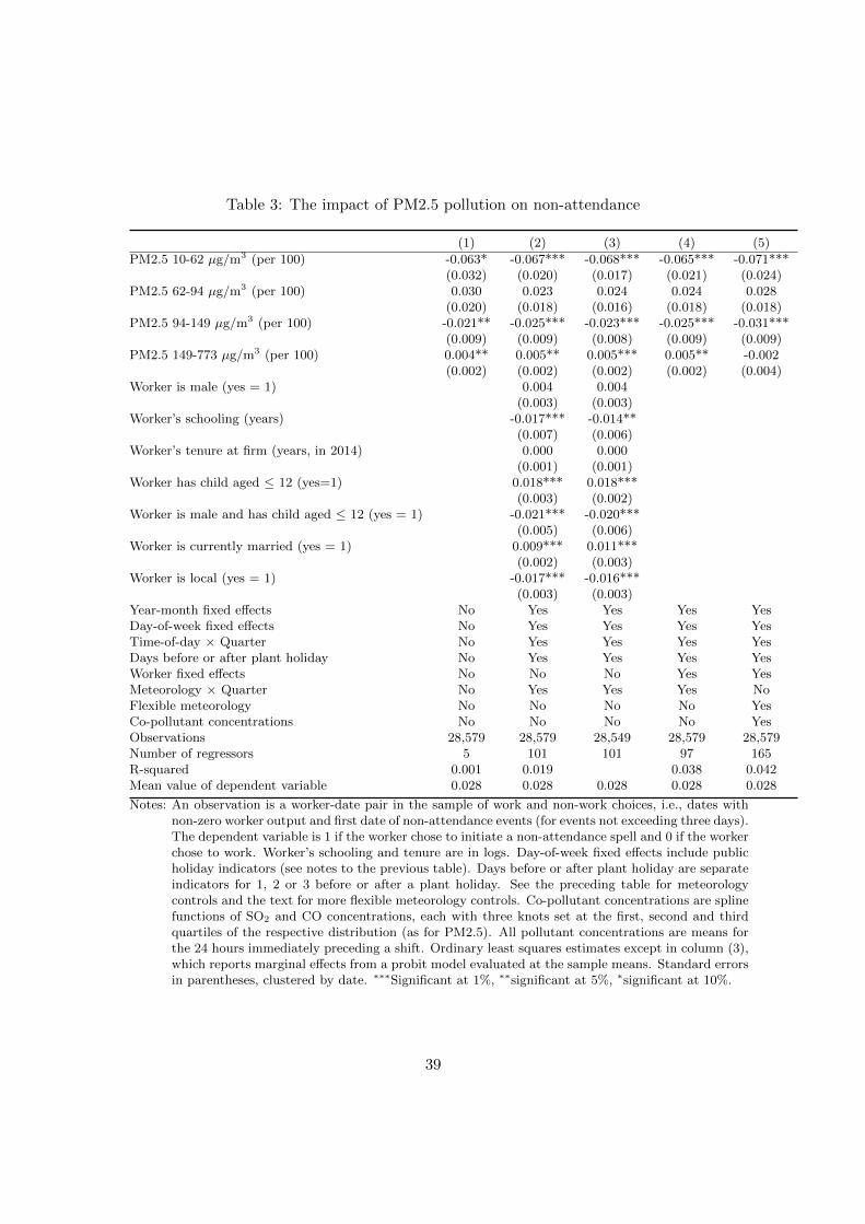
Table 3: The impact of PM2.5 pollution on non-attendance
(1) (2) (3) (4) (5)
PM2.5 10-62 µg/m3 (per 100) -0.063* -0.067*** -0.068*** -0.065*** -0.071***(0.032) (0.020) (0.017) (0.021) (0.024)
PM2.5 62-94 µg/m3 (per 100) 0.030 0.023 0.024 0.024 0.028(0.020) (0.018) (0.016) (0.018) (0.018)
PM2.5 94-149 µg/m3 (per 100) -0.021** -0.025*** -0.023*** -0.025*** -0.031***(0.009) (0.009) (0.008) (0.009) (0.009)
PM2.5 149-773 µg/m3 (per 100) 0.004** 0.005** 0.005*** 0.005** -0.002(0.002) (0.002) (0.002) (0.002) (0.004)
Worker is male (yes = 1) 0.004 0.004(0.003) (0.003)
Worker’s schooling (years) -0.017*** -0.014**(0.007) (0.006)
Worker’s tenure at firm (years, in 2014) 0.000 0.000(0.001) (0.001)
Worker has child aged ≤ 12 (yes=1) 0.018*** 0.018***(0.003) (0.002)
Worker is male and has child aged ≤ 12 (yes = 1) -0.021*** -0.020***(0.005) (0.006)
Worker is currently married (yes = 1) 0.009*** 0.011***(0.002) (0.003)
Worker is local (yes = 1) -0.017*** -0.016***(0.003) (0.003)
Year-month fixed effects No Yes Yes Yes YesDay-of-week fixed effects No Yes Yes Yes YesTime-of-day × Quarter No Yes Yes Yes YesDays before or after plant holiday No Yes Yes Yes YesWorker fixed effects No No No Yes YesMeteorology × Quarter No Yes Yes Yes NoFlexible meteorology No No No No YesCo-pollutant concentrations No No No No YesObservations 28,579 28,579 28,549 28,579 28,579Number of regressors 5 101 101 97 165R-squared 0.001 0.019 0.038 0.042Mean value of dependent variable 0.028 0.028 0.028 0.028 0.028
Notes: An observation is a worker-date pair in the sample of work and non-work choices, i.e., dates withnon-zero worker output and first date of non-attendance events (for events not exceeding three days).The dependent variable is 1 if the worker chose to initiate a non-attendance spell and 0 if the workerchose to work. Worker’s schooling and tenure are in logs. Day-of-week fixed effects include publicholiday indicators (see notes to the previous table). Days before or after plant holiday are separateindicators for 1, 2 or 3 before or after a plant holiday. See the preceding table for meteorologycontrols and the text for more flexible meteorology controls. Co-pollutant concentrations are splinefunctions of SO2 and CO concentrations, each with three knots set at the first, second and thirdquartiles of the respective distribution (as for PM2.5). All pollutant concentrations are means forthe 24 hours immediately preceding a shift. Ordinary least squares estimates except in column (3),which reports marginal effects from a probit model evaluated at the sample means. Standard errorsin parentheses, clustered by date. ∗∗∗Significant at 1%, ∗∗significant at 5%, ∗significant at 10%.
39
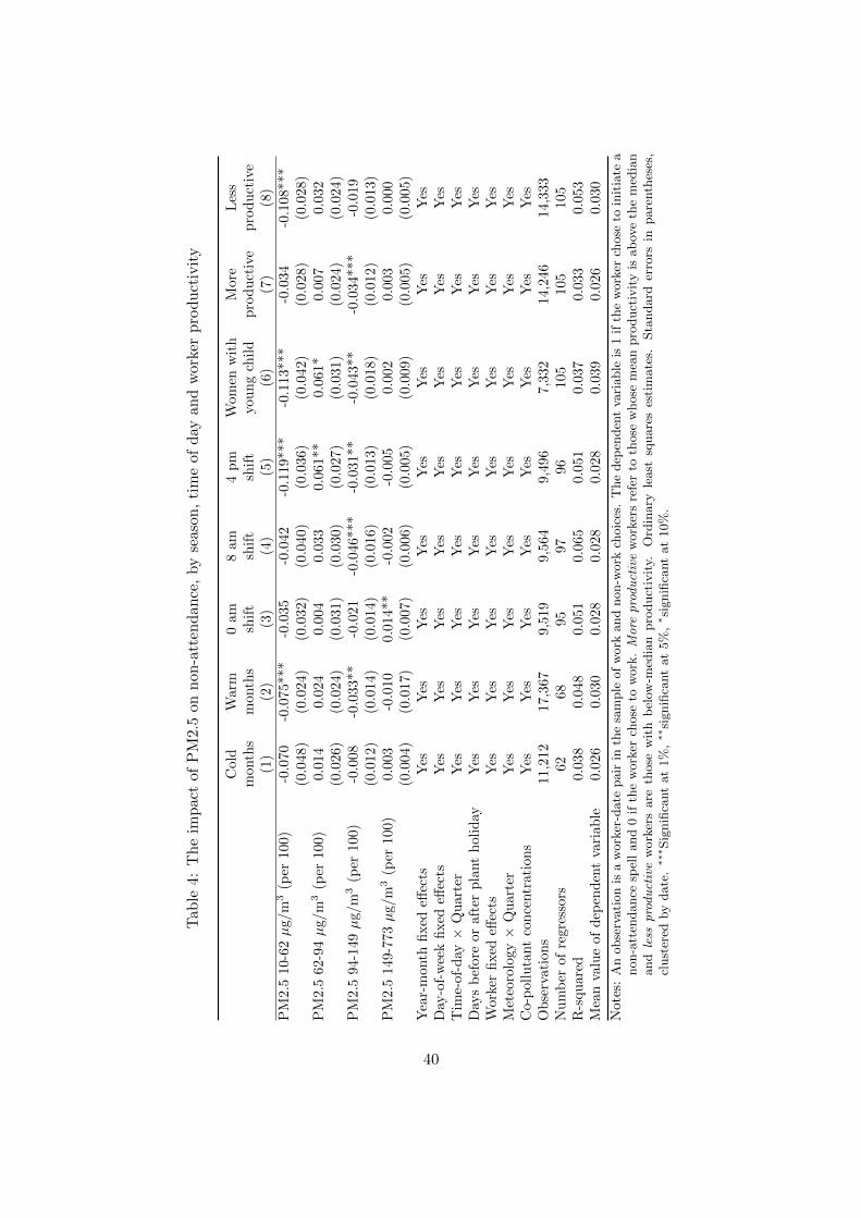
Tab
le4:
Th
eim
pact
ofP
M2.5
on
non
-att
end
ance
,by
seas
on,
tim
eof
day
and
wor
ker
pro
du
ctiv
ity
Col
dW
arm
0am
8am
4p
mW
om
enw
ith
More
Les
sm
onth
sm
onth
ssh
ift
shif
tsh
ift
you
ng
chil
dp
rod
uct
ive
pro
du
ctiv
e(1
)(2
)(3
)(4
)(5
)(6
)(7
)(8
)P
M2.
510
-62µ
g/m
3(p
er10
0)-0
.070
-0.0
75***
-0.0
35
-0.0
42
-0.1
19***
-0.1
13***
-0.0
34
-0.1
08***
(0.0
48)
(0.0
24)
(0.0
32)
(0.0
40)
(0.0
36)
(0.0
42)
(0.0
28)
(0.0
28)
PM
2.5
62-9
4µ
g/m
3(p
er10
0)0.
014
0.0
24
0.0
04
0.0
33
0.0
61**
0.0
61*
0.0
07
0.0
32
(0.0
26)
(0.0
24)
(0.0
31)
(0.0
30)
(0.0
27)
(0.0
31)
(0.0
24)
(0.0
24)
PM
2.5
94-1
49µ
g/m
3(p
er10
0)-0
.008
-0.0
33**
-0.0
21
-0.0
46***
-0.0
31**
-0.0
43**
-0.0
34***
-0.0
19
(0.0
12)
(0.0
14)
(0.0
14)
(0.0
16)
(0.0
13)
(0.0
18)
(0.0
12)
(0.0
13)
PM
2.5
149-
773µ
g/m
3(p
er10
0)0.
003
-0.0
10
0.0
14**
-0.0
02
-0.0
05
0.0
02
0.0
03
0.0
00
(0.0
04)
(0.0
17)
(0.0
07)
(0.0
06)
(0.0
05)
(0.0
09)
(0.0
05)
(0.0
05)
Yea
r-m
onth
fixed
effec
tsY
esY
esY
esY
esY
esY
esY
esY
esD
ay-o
f-w
eek
fixed
effec
tsY
esY
esY
esY
esY
esY
esY
esY
esT
ime-
of-d
ay×
Qu
arte
rY
esY
esY
esY
esY
esY
esY
esY
esD
ays
bef
ore
oraf
ter
pla
nt
hol
iday
Yes
Yes
Yes
Yes
Yes
Yes
Yes
Yes
Wor
ker
fixed
effec
tsY
esY
esY
esY
esY
esY
esY
esY
esM
eteo
rolo
gy×
Qu
arte
rY
esY
esY
esY
esY
esY
esY
esY
esC
o-p
ollu
tant
con
centr
atio
ns
Yes
Yes
Yes
Yes
Yes
Yes
Yes
Yes
Ob
serv
atio
ns
11,2
1217,3
67
9,5
19
9,5
64
9,4
96
7,3
32
14,2
46
14,3
33
Nu
mb
erof
regr
esso
rs62
68
95
97
96
105
105
105
R-s
qu
ared
0.03
80.0
48
0.0
51
0.0
65
0.0
51
0.0
37
0.0
33
0.0
53
Mea
nva
lue
ofd
epen
den
tva
riab
le0.
026
0.0
30
0.0
28
0.0
28
0.0
28
0.0
39
0.0
26
0.0
30
Not
es:
An
obse
rvati
on
isa
work
er-d
ate
pair
inth
esa
mple
of
work
and
non-w
ork
choic
es.
The
dep
enden
tva
riable
is1
ifth
ew
ork
erch
ose
toin
itia
tea
non-a
tten
dance
spel
land
0if
the
work
erch
ose
tow
ork
.More
productive
work
ers
refe
rto
those
whose
mea
npro
duct
ivit
yis
ab
ove
the
med
ian
and
less
productive
work
ers
are
those
wit
hb
elow
-med
ian
pro
duct
ivit
y.O
rdin
ary
least
square
ses
tim
ate
s.Sta
ndard
erro
rsin
pare
nth
eses
,cl
ust
ered
by
date
.∗∗
∗Sig
nifi
cant
at
1%
,∗∗
signifi
cant
at
5%
,∗si
gnifi
cant
at
10%
.
40
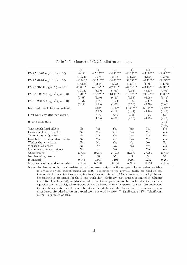
Table 5: The impact of PM2.5 pollution on output
(1) (2) (3) (4) (5) (6)
PM2.5 10-62 µg/m3 (per 100) -24.52 -45.02*** -44.41*** -40.13*** -43.49*** -39.86***(19.22) (14.34) (14.18) (12.28) (12.56) (12.30)
PM2.5 62-94 µg/m3 (per 100) -36.01** -33.71*** -34.21*** -39.08*** -40.73*** -39.28***(15.68) (12.44) (12.33) (10.97) (11.09) (11.00)
PM2.5 94-149 µg/m3 (per 100) -43.83*** -48.35*** -47.90*** -44.38*** -43.18*** -44.35***(10.12) (8.69) (8.63) (7.92) (8.23) (7.94)
PM2.5 149-230 µg/m3 (per 100) -20.61*** -16.67*** -16.91*** -18.07*** -19.84*** -18.02***(7.58) (6.40) (6.37) (5.58) (6.06) (5.54)
PM2.5 230-773 µg/m3 (per 100) -1.76 -0.70 -0.70 -1.34 -4.96* -1.36(2.12) (1.99) (2.00) (2.06) (2.79) (2.06)
Last work day before non-attend. 9.34* 10.55** 11.94*** 12.11*** 11.92***(5.17) (5.18) (4.44) (4.46) (4.43)
First work day after non-attend. -4.72 -3.55 -3.26 -3.22 -3.27(4.65) (4.67) (4.15) (4.15) (4.15)
Inverse Mills ratio 0.34(1.59)
Year-month fixed effects No Yes Yes Yes Yes YesDay-of-week fixed effects No Yes Yes Yes Yes YesTime-of-day × Quarter No Yes Yes Yes Yes YesDays before or after plant holiday No Yes Yes Yes Yes YesWorker characteristics No No Yes No No NoWorker fixed effects No No No Yes Yes YesCo-pollutant concentrations No No No No Yes YesObservations 27,673 27,673 27,673 27,673 27,585 27,673Number of regressors 6 48 55 49 59 50R-squared 0.045 0.099 0.103 0.281 0.282 0.281Mean value of dependent variable 509.04 509.04 509.04 509.04 508.94 509.04
Notes: An observation is a worker-date pair with non-zero output in the sample. The dependent variableis a worker’s total output during her shift. See notes to the previous tables for fixed effects.Co-pollutant concentrations are spline functions of SO2 and CO concentrations. All pollutantconcentrations are means for the 8-hour work shift. Ordinary least squares estimates in columns(1) to (5). In column (6), variables excluded from the output equation but included in the selectionequation are meteorological conditions that are allowed to vary by quarter of year. We implementthe selection equation at the monthly rather than daily level due to the lack of variation in non-attendance. Standard errors in parentheses, clustered by date. ∗∗∗Significant at 1%, ∗∗significantat 5%, ∗significant at 10%.
41
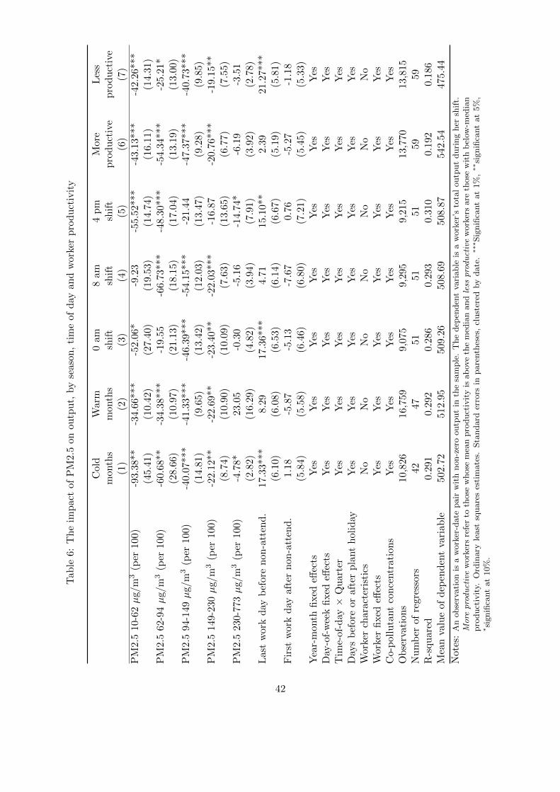
Tab
le6:
Th
eim
pact
ofP
M2.
5on
outp
ut,
by
seas
on,
tim
eof
day
and
wor
ker
pro
du
ctiv
ity
Cold
War
m0
am8
am4
pm
Mor
eL
ess
mon
ths
mon
ths
shif
tsh
ift
shif
tp
rod
uct
ive
pro
du
ctiv
e(1
)(2
)(3
)(4
)(5
)(6
)(7
)
PM
2.5
10-
62µ
g/m
3(p
er10
0)-9
3.3
8**
-34.
66**
*-5
2.06
*-9
.23
-55.
52**
*-4
3.13
***
-42.
26**
*(4
5.4
1)(1
0.42
)(2
7.40
)(1
9.53
)(1
4.74
)(1
6.11
)(1
4.31
)P
M2.5
62-
94µ
g/m
3(p
er10
0)-6
0.6
8**
-34.
38**
*-1
9.55
-66.
73**
*-4
8.30
***
-54.
34**
*-2
5.21
*(2
8.6
6)(1
0.97
)(2
1.13
)(1
8.15
)(1
7.04
)(1
3.19
)(1
3.00
)P
M2.5
94-
149µ
g/m
3(p
er10
0)-4
0.0
7***
-41.
33**
*-4
6.39
***
-54.
15**
*-2
1.44
-47.
37**
*-4
0.73
***
(14.
81)
(9.6
5)(1
3.42
)(1
2.03
)(1
3.47
)(9
.28)
(9.8
5)P
M2.
514
9-23
0µ
g/m
3(p
er100
)-2
2.1
2**
-22.
69**
-23.
40**
-22.
03**
*-1
6.87
-20.
76**
*-1
9.15
**(8
.74)
(10.
90)
(10.
09)
(7.6
3)(1
3.65
)(6
.77)
(7.5
5)P
M2.
523
0-77
3µ
g/m
3(p
er100
)-4
.78*
23.0
5-0
.30
-5.1
6-1
4.74
*-6
.19
-3.5
1(2
.82)
(16.
29)
(4.8
2)(3
.94)
(7.9
1)(3
.92)
(2.7
8)L
ast
wor
kd
ayb
efore
non
-att
end
.17.
33**
*8.
2917
.36*
**4.
7115
.10*
*2.
3921
.27*
**(6
.10)
(6.0
8)(6
.53)
(6.1
4)(6
.67)
(5.1
9)(5
.81)
Fir
stw
ork
day
afte
rn
on-a
tten
d.
1.1
8-5
.87
-5.1
3-7
.67
0.76
-5.2
7-1
.18
(5.8
4)
(5.5
8)(6
.46)
(6.8
0)(7
.21)
(5.4
5)(5
.33)
Yea
r-m
onth
fixed
effec
tsY
esY
esY
esY
esY
esY
esY
esD
ay-o
f-w
eek
fixed
effec
tsY
esY
esY
esY
esY
esY
esY
esT
ime-
of-d
ay×
Qu
art
erY
esY
esY
esY
esY
esY
esY
esD
ays
bef
ore
oraft
erp
lant
hol
iday
Yes
Yes
Yes
Yes
Yes
Yes
Yes
Work
erch
ara
cter
isti
csN
oN
oN
oN
oN
oN
oN
oW
ork
erfi
xed
effec
tsY
esY
esY
esY
esY
esY
esY
esC
o-p
oll
uta
nt
con
centr
ati
on
sY
esY
esY
esY
esY
esY
esY
esO
bse
rvat
ion
s10
,826
16,7
599,
075
9,29
59,
215
13,7
7013
,815
Nu
mb
erof
regre
ssor
s42
4751
5151
5959
R-s
qu
ared
0.2
910.
292
0.28
60.
293
0.31
00.
192
0.18
6M
ean
valu
eof
dep
end
ent
vari
able
502.
7251
2.95
509.
2650
8.69
508.
8754
2.54
475.
44
Note
s:A
nobse
rvati
on
isa
work
er-d
ate
pair
wit
hnon-z
ero
outp
ut
inth
esa
mple
.T
he
dep
enden
tva
riable
isa
work
er’s
tota
loutp
ut
duri
ng
her
shif
t.More
productive
work
ers
refe
rto
those
whose
mea
npro
duct
ivit
yis
ab
ove
the
med
ian
andless
productive
work
ers
are
those
wit
hb
elow
-med
ian
pro
duct
ivit
y.O
rdin
ary
least
square
ses
tim
ate
s.Sta
ndard
erro
rsin
pare
nth
eses
,cl
ust
ered
by
date
.∗∗
∗Sig
nifi
cant
at
1%
,∗∗
signifi
cant
at
5%
,∗si
gnifi
cant
at
10%
.
42
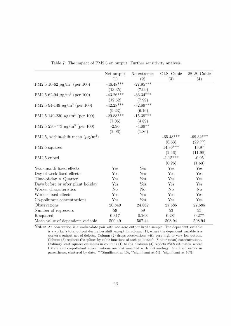
Table 7: The impact of PM2.5 on output: Further sensitivity analysis
Net output No extremes OLS, Cubic 2SLS, Cubic(1) (2) (3) (4)
PM2.5 10-62 µg/m3 (per 100) -46.48*** -27.95***(13.35) (7.99)
PM2.5 62-94 µg/m3 (per 100) -43.26*** -36.34***(12.62) (7.99)
PM2.5 94-149 µg/m3 (per 100) -42.28*** -32.89***(9.23) (6.16)
PM2.5 149-230 µg/m3 (per 100) -29.88*** -15.39***(7.06) (4.89)
PM2.5 230-773 µg/m3 (per 100) -2.96 -4.09**(2.96) (1.86)
PM2.5, within-shift mean (µg/m3) -65.48*** -69.32***(6.63) (22.77)
PM2.5 squared 14.86*** 13.97(2.46) (11.98)
PM2.5 cubed -1.15*** -0.95(0.26) (1.63)
Year-month fixed effects Yes Yes Yes YesDay-of-week fixed effects Yes Yes Yes YesTime-of-day × Quarter Yes Yes Yes YesDays before or after plant holiday Yes Yes Yes YesWorker characteristics No No No NoWorker fixed effects Yes Yes Yes YesCo-pollutant concentrations Yes Yes Yes YesObservations 20,849 24,862 27,585 27,585Number of regressors 59 59 53 53R-squared 0.317 0.263 0.281 0.277Mean value of dependent variable 500.49 507.44 508.94 508.94
Notes: An observation is a worker-date pair with non-zero output in the sample. The dependent variableis a worker’s total output during her shift, except for column (1), where the dependent variable is aworker’s output net of defects. Column (2) drops observations with very high or very low output.Column (3) replaces the splines by cubic functions of each pollutant’s (8-hour mean) concentrations.Ordinary least squares estimates in columns (1) to (3). Column (4) reports 2SLS estimates, wherePM2.5 and co-pollutant concentrations are instrumented with meteorology. Standard errors inparentheses, clustered by date. ∗∗∗Significant at 1%, ∗∗significant at 5%, ∗significant at 10%.
43
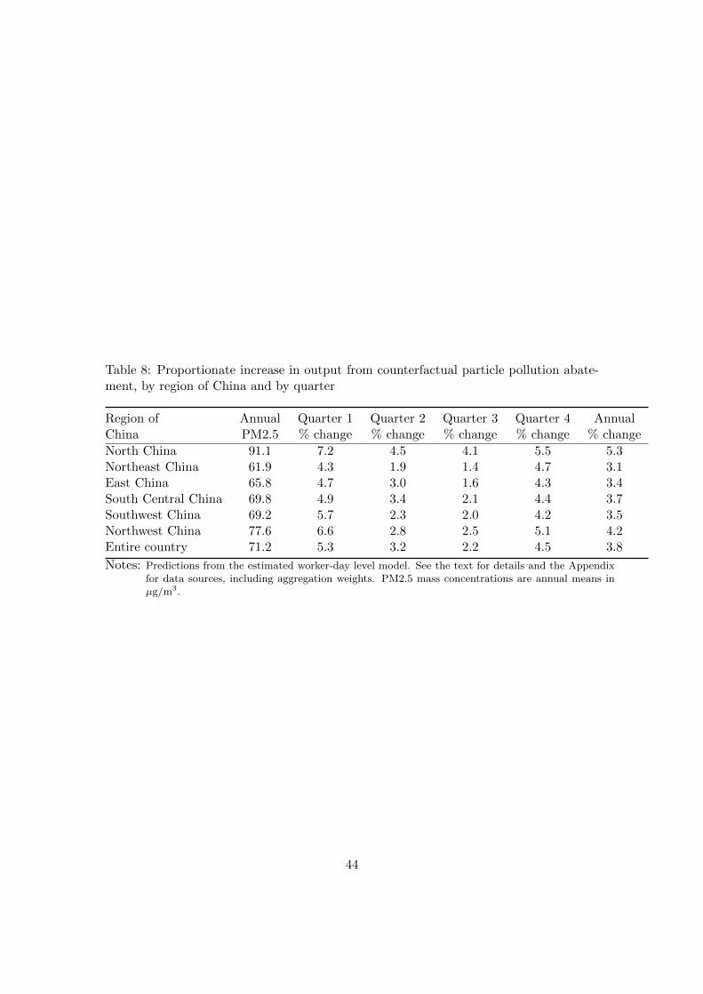
Table 8: Proportionate increase in output from counterfactual particle pollution abate-ment, by region of China and by quarter
Region of Annual Quarter 1 Quarter 2 Quarter 3 Quarter 4 AnnualChina PM2.5 % change % change % change % change % change
North China 91.1 7.2 4.5 4.1 5.5 5.3Northeast China 61.9 4.3 1.9 1.4 4.7 3.1East China 65.8 4.7 3.0 1.6 4.3 3.4South Central China 69.8 4.9 3.4 2.1 4.4 3.7Southwest China 69.2 5.7 2.3 2.0 4.2 3.5Northwest China 77.6 6.6 2.8 2.5 5.1 4.2Entire country 71.2 5.3 3.2 2.2 4.5 3.8
Notes: Predictions from the estimated worker-day level model. See the text for details and the Appendixfor data sources, including aggregation weights. PM2.5 mass concentrations are annual means inµg/m3.
44
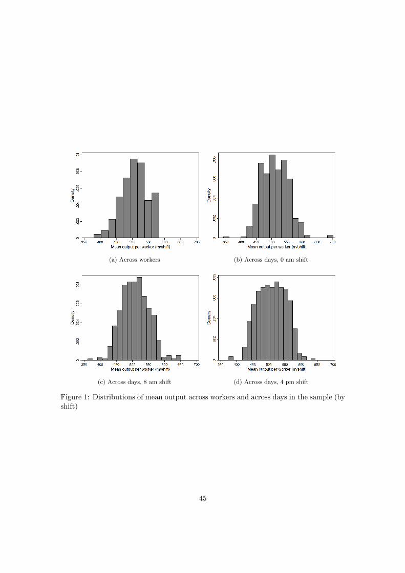
(a) Across workers (b) Across days, 0 am shift
(c) Across days, 8 am shift (d) Across days, 4 pm shift
Figure 1: Distributions of mean output across workers and across days in the sample (byshift)
45
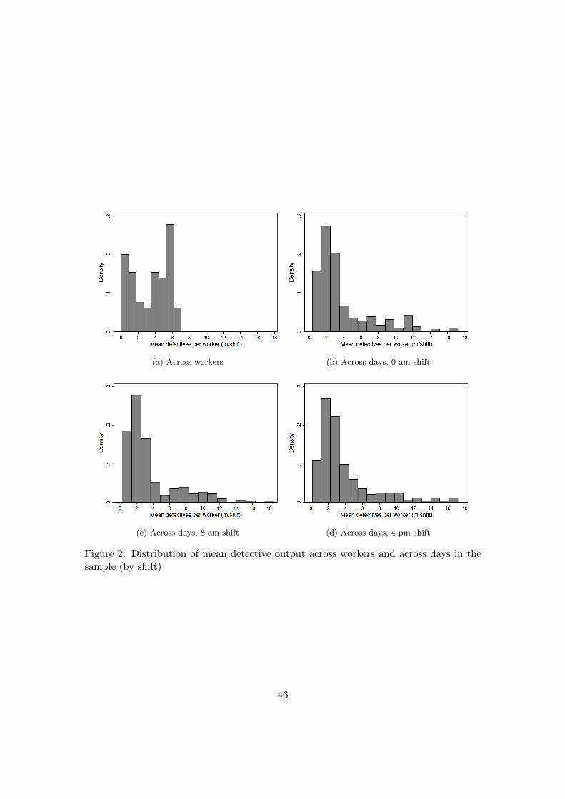
(a) Across workers (b) Across days, 0 am shift
(c) Across days, 8 am shift (d) Across days, 4 pm shift
Figure 2: Distribution of mean detective output across workers and across days in thesample (by shift)
46
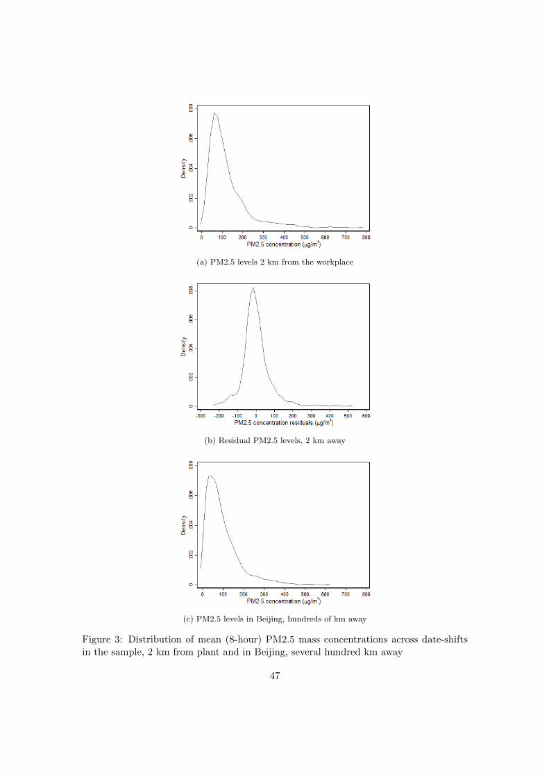
(a) PM2.5 levels 2 km from the workplace
(b) Residual PM2.5 levels, 2 km away
(c) PM2.5 levels in Beijing, hundreds of km away
Figure 3: Distribution of mean (8-hour) PM2.5 mass concentrations across date-shiftsin the sample, 2 km from plant and in Beijing, several hundred km away
47
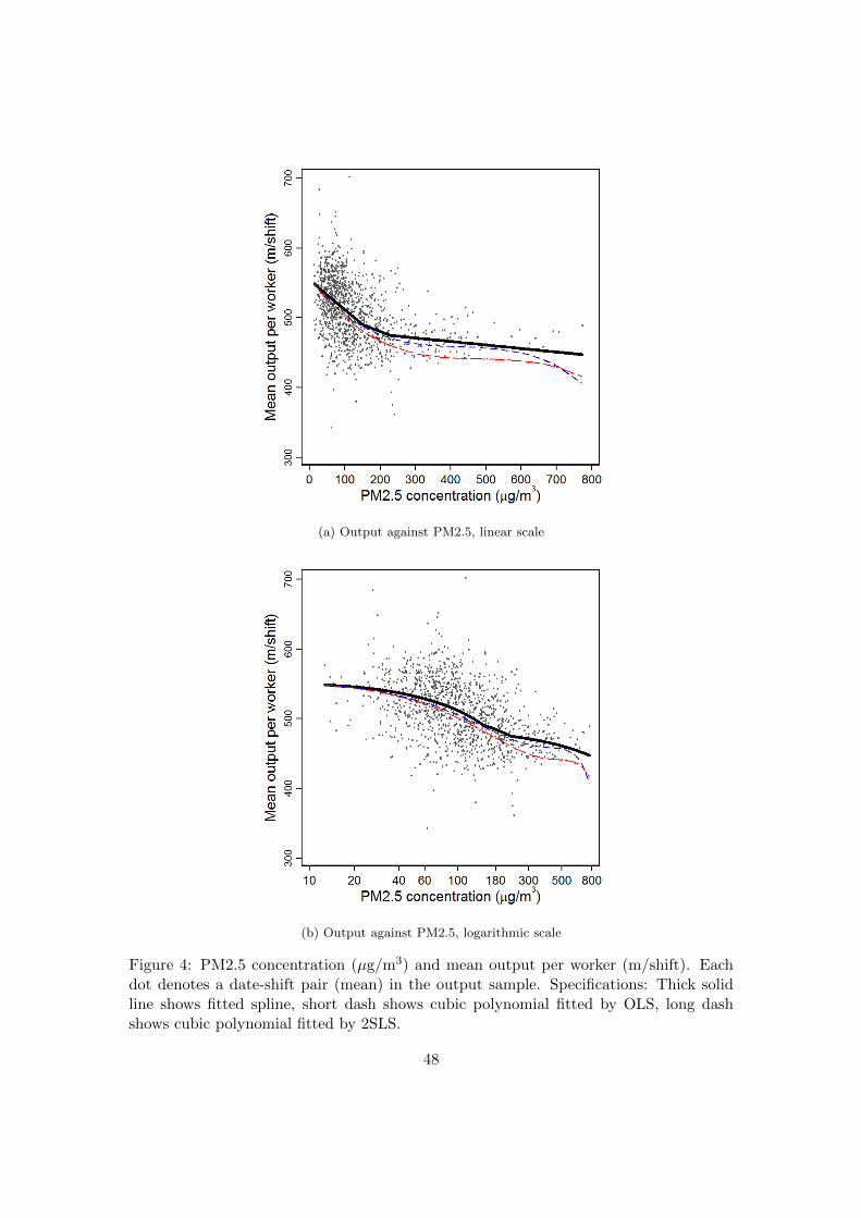
(a) Output against PM2.5, linear scale
(b) Output against PM2.5, logarithmic scale
Figure 4: PM2.5 concentration (µg/m3) and mean output per worker (m/shift). Eachdot denotes a date-shift pair (mean) in the output sample. Specifications: Thick solidline shows fitted spline, short dash shows cubic polynomial fitted by OLS, long dashshows cubic polynomial fitted by 2SLS.
48
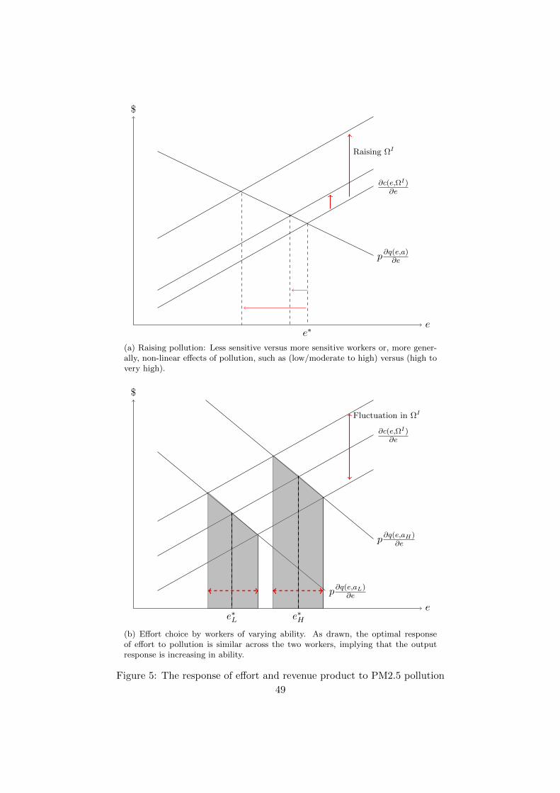
$
e
p∂q(e,a)∂e
∂c(e,ΩI)∂e
e∗
Raising ΩI
(a) Raising pollution: Less sensitive versus more sensitive workers or, more gener-ally, non-linear effects of pollution, such as (low/moderate to high) versus (high tovery high).
$
e
∂c(e,ΩI)∂e
p∂q(e,aH)∂e
p∂q(e,aL)∂e
Fluctuation in ΩI
e∗He∗L
(b) Effort choice by workers of varying ability. As drawn, the optimal responseof effort to pollution is similar across the two workers, implying that the outputresponse is increasing in ability.
Figure 5: The response of effort and revenue product to PM2.5 pollution
49
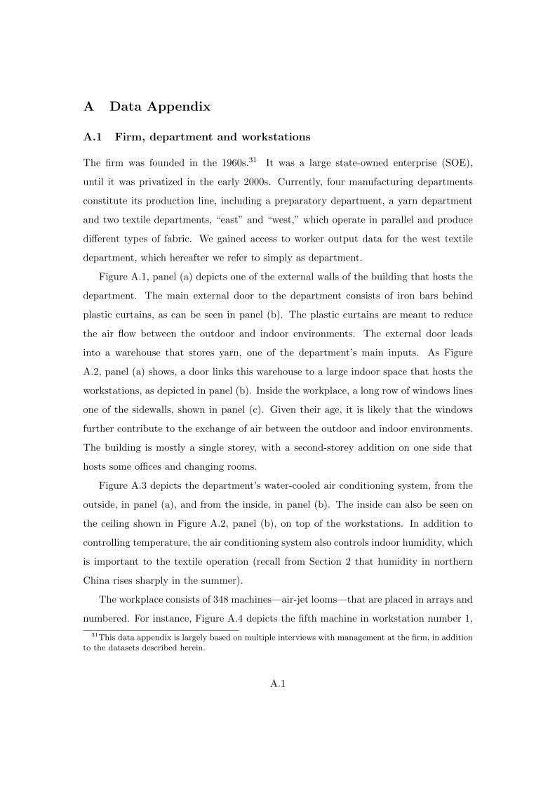
A Data Appendix
A.1 Firm, department and workstations
The firm was founded in the 1960s.31 It was a large state-owned enterprise (SOE),
until it was privatized in the early 2000s. Currently, four manufacturing departments
constitute its production line, including a preparatory department, a yarn department
and two textile departments, “east” and “west,” which operate in parallel and produce
different types of fabric. We gained access to worker output data for the west textile
department, which hereafter we refer to simply as department.
Figure A.1, panel (a) depicts one of the external walls of the building that hosts the
department. The main external door to the department consists of iron bars behind
plastic curtains, as can be seen in panel (b). The plastic curtains are meant to reduce
the air flow between the outdoor and indoor environments. The external door leads
into a warehouse that stores yarn, one of the department’s main inputs. As Figure
A.2, panel (a) shows, a door links this warehouse to a large indoor space that hosts the
workstations, as depicted in panel (b). Inside the workplace, a long row of windows lines
one of the sidewalls, shown in panel (c). Given their age, it is likely that the windows
further contribute to the exchange of air between the outdoor and indoor environments.
The building is mostly a single storey, with a second-storey addition on one side that
hosts some offices and changing rooms.
Figure A.3 depicts the department’s water-cooled air conditioning system, from the
outside, in panel (a), and from the inside, in panel (b). The inside can also be seen on
the ceiling shown in Figure A.2, panel (b), on top of the workstations. In addition to
controlling temperature, the air conditioning system also controls indoor humidity, which
is important to the textile operation (recall from Section 2 that humidity in northern
China rises sharply in the summer).
The workplace consists of 348 machines—air-jet looms—that are placed in arrays and
numbered. For instance, Figure A.4 depicts the fifth machine in workstation number 1,
31This data appendix is largely based on multiple interviews with management at the firm, in additionto the datasets described herein.
A.1
labeled 1-5. The machines were purchased from Toyota in the early 2000s, when the
firm was restructured. The technical specifications under which looms operate are set by
the firm’s engineers/technicians. In principle, a workstation comprised of 10 looms can
produce as much as 780 meters of 133-type fabric during an 8-hour shift, or about 760
m if set up to produce 134-type fabric. In practice, output will be lower because threads
naturally break, requiring that the worker reconnect them while the machine lies idle.
While the median output in our sample is 506 m per worker-shift, we observe some
worker-shifts with substantially higher output levels (the maximum is as high as 1,137
m). Such high levels of output exceed the nominal capacity of a workstation over an 8-
hour period. On enquiring with management, we were informed that while unusual, there
are cases of workers who request an extension of their work hours into the subsequent
shift, subject to approval by the subsequent shift’s supervisor and pending availability
of workstations. While the overtime output is combined and recorded with the worker’s
output during her standard 8-hour shift, such extended work hours are unfortunately
not recorded (likely because such occasions are exceptional). For this reason, we conduct
robustness tests in which we either drop worker-shift observations with output above the
95th percentile, or replace the observed output values by 780 m.
Looms producing one type of fabric (133 or 134) can be readjusted to produce the
other type by the firm’s technicians (this involves dropping wares, changing operating
parameters, etc). In practice, a single workstation will be set up to produce only one type
of fabric. This is because a worker needs to attentively observe the number of warps,
which varies across fabric type, and simultaneously operating looms producing different
fabric types would be too taxing on the worker. Over our sample period, two-fifths of
machines were set up to produce fabric of type 133, with the remaining producing 134.
Given the nature of materials being handled, ambient air that the workers are ex-
posed to contains not only fine particles (i.e., less than 2.5 µm in diameter) from the
outdoor environment but also, to some degree, cotton dust. Cotton dust consists of
coarse, not fine, particles; however, cotton dust is a researched occupational hazard.32
32World Health Organization (1999) classifies cotton dust in the “thoracic particulate fraction,” i.e.,particles of diameter up to 25 µm in diameter (10 times larger than PM2.5), which can penetrate the
A.2
While workers in our sample are less exposed to cotton dust than those in the prepara-
tory department, we cannot rule out the possibility that cotton dust in ambient air
impacts output. Presumably, higher output levels across the department raise the con-
centration of cotton dust in indoor air. In the event that higher concentrations of cotton
dust adversely affect output, and that this relationship holds for day-to-day variation in
ambient dust concentrations, our estimates of the adverse effect of PM2.5 concentrations
on output will be a lower bound.
There is no combustion inside the department, and the department does not handle
chemicals (which if volatile might evaporate and contribute to the formation of particles).
Thus, indoor PM2.5 pollution originates from the outdoor environment.
A.2 Workers, output, holidays and non-attendance
Worker characteristics were obtained from both the human resources department (birth
year, gender, schooling, hometown, contract, etc) and the “family planning” department
(number of children, their birth year, etc). We accessed such data already in digital
form.
In the sample, contract duration positively correlates with a worker’s tenure at the
firm. In addition, workers with longer tenure (above 10 years) are eligible to purchase
housing at subsidizes rates in the vicinity of the plant. Single workers with less work
years at the firm typically live in dorms located inside the industrial complex.
At the end of her shift, a worker marks the point at which her production ended. The
completed rolls of fabric are then inspected for defects and output is recorded. Panel (a)
of Figure A.5 depicts the quality control process. Panel (b) illustrates the output records
for three different workers, by date-shift, during a month. For a worker, the first column
records total output in meters, whereas the second column records defective output. We
obtained temporary access to these paper records (a different booklet per month per
team), through an administrative department where they are kept, and proceeded to
digitize them.
airways of the lung and cause airway disease. Christiani et al. (1999) examine the long-term decline inlung function among cotton workers.
A.3
A team supervisor’s main task is to oversee her workers and assist them during the
shift. The supervisor rotates, along with the rest of her team, among the different shift
times. A supervisor’s salary is partly fixed, partly variable. The variable component of
a supervisor’s compensation is determined by the average output of her team’s workers.
Based on output records, we observe workers who join the department after the
sample period begins, as well as workers who leave the department before the sample
period ends. This change in the workforce is reported in Figure A.6 by team. As
mentioned in Section 2, early fall 2013 was the time with most turnover in the sample
(particularly Team 2), as well as the point in which the piece rate was increased, from
0.07 to 0.10 CNY per meter of (133-equivalent) fabric. We find workers who joined the
department after the wage raise to be 21 m/shift (about 4.3%) more productive than
workers who left the department before the raise; a test of equality of means is rejected
at the 1% significance level.33
Table A.1 lists dates with zero output in the department (which we label plant holi-
days) alongside public holidays. Though plant holidays are usually set around the official
holiday calendar, they only partially overlap with public holidays as they depend on the
production schedule. A robustness test we conduct is to drop observations pertaining to
dates on the official holiday calendar that were not observed by the department as well
as up to three days before and up to three days after public holidays.
Dates in which output records show positive output for a worker are labeled atten-
dance dates. In addition to plant holidays, output records indicate zero output for specific
workers on specific dates—we label these non-attendance dates. Figure A.7 indicates the
rates of work attendance across dates and across workers, respectively. For 94% of dates
in the sample (other than plant holidays), more than nine-tenths of the workforce attends
work. On one isolated date, May 9, 2013, only three-quarters of the workers have positive
output—we do not know what happened that day. (Our estimation results are robust to
dropping this date from the sample.) Most workers in the sample have attendance rates
exceeding 90%, noting that non-attendance includes planned leave (recall that we are
33Comparing these new workers to workers who are in the sample throughout the entire period, theformer group’s output is slightly lower, presumably due to learning.
A.4
unable to distinguish between planned and unplanned non-attendance). Three workers
in the sample never take leave (beyond the 54 days of plant holiday). Figure A.9 plots
rates of non-attendance against mean PM2.5 concentrations on dates in our sample.
A.3 Air pollution and meteorology
We obtained data from several sources. Hourly readings for pollutant mass concen-
trations (PM2.5, PM10, SO2, CO, NO2, and O3) at four Chinese Ministry of Envi-
ronmental Protection sites located in the city where the firm is based are available at
www.cnpm2d5.com/. Hourly readings for PM2.5 mass concentrations at US Embassies
in Beijing, Chengdu, Guangzhou, Shanghai and Shenyang are available from the US De-
partment of State at www.stateair.net/web/historical/1/1.html. Meteorological
conditions measured in the city where the firm is based come from two sources: (i) 3-
hourly readings for ground temperature, humidity, atmospheric pressure, precipitation,
wind speed and wind direction are available at www.worldweatheronline.com; and (ii)
daily readings for ground temperature (maximum and minimum), precipitation, wind
speed and wind direction are available at www.lishi.tianqi.com (these are based on
readings by the National Meteorological Center).
We inspected pollutant concentrations, reading by reading, and did minimal imput-
ing with regard to the raw data. Specifically, for the closest PM2.5 monitor, 58 date-hour
observations out of a total of 10,186 non-missing observations over the sample period
(April 2013 to June 2014) were recoded as missing, largely because values over adjacent
hours were invariant at 3 or at 1000 µg/m3. Our results are robust to not recoding these
0.6% of observations (a spreadsheet listing the raw data and the 58 recoded values is
available from the authors). Table A.2 shows that the availability of PM2.5 measure-
ments is high and fairly balanced over months of year and hours of day. For example,
data availability ranges from 99% of possible date-hour measurements in January to 82%
in November, and from 96% at 7 pm to 87% at 12 pm. Table A.3 indicates the increased
data availability when using the mean concentration at the three other nearby PM2.5
monitors to impute for a missing value at the nearest monitor at a given date-hour. For
A.5
example, data availability in November increases by 14 percentage points. Table A.4
reports the very high correlation between hourly PM2.5 at the four monitoring sites, all
located up to 5 km from the plant. The table also reports correlation coefficients between
these hourly PM2.5 concentration measurements, in the city where the firm is based, and
measurements at the US Embassy in Beijing and in Shenyang. For perspective, our city
of study, Beijing and Shenyang are all within several hundred km of each other. We
also recoded to missing a few date-hour readings with negative concentrations in the US
Department of State data.
Figure A.10 plots daily mean PM2.5 concentrations over our sample period at the
monitoring site located 2 km from the plant and in Beijing, respectively. Given some very
high measurements in the winter, these plots are reproduced in Figure A.11 restricting
the vertical axis to no more than 400 µg/m3. Compared to Beijing, particle pollution
in the city we examine tends to be higher, while both locations follow a similar annual
pattern.
We similarly inspected measured concentrations for pollutants other than PM2.5.
In the case of SO2, we recoded as missing 0.04% of all original non-missing date-hour
observations. No recoding seemed called for in the case of CO. Whereas for CO our
analysis uses readings at the site located 2 km from the plant, in the case of SO2 we use
the mean reading across all four city monitors, since the closest monitor exhibits some
periods of low values and low variability. A spreadsheet comparing the raw individual
data to the cross-monitor means is available from the authors.
Meteorological data was missing for only one date in the sample period, September
6, 2013, and only for the 24-hour dataset. Except for wind direction, where we use
daily observations, our analysis uses meteorological data from the higher-frequency (3-
hour) dataset, though we ensured that both data sources are in broad agreement. For
example, Figure A.12 shows that mean daily temperatures as recorded in the 3-hourly
data correlate tightly with those in the daily dataset.
Analysis of residuals: Worker output, PM2.5 concentration and temper-
ature. We separately regress output (mean across workers), PM2.5 concentration, and
A.6
temperature, averaged at the date-shift level, on calendar-month, day-of-week (including
public holiday indicators) and time-of-day×quarter fixed effects. We note that the R2 for
the temperature regression is over double that for the PM2.5 concentration regression,
respectively, R2 of 88% and 39%, suggesting that seasonal, weekly and diurnal cycles
(both natural and anthropogenic) are highly predictive of temperature, while PM2.5
concentrations show more orthogonal variation. We obtain fitted residuals for each of
these three regressions and plot them in Figure A.13, namely worker output against
PM2.5 in panel (a), and mean worker output (again) against temperature in panel (b).
The strong negative relationship between output and fine-particle pollution—even when
time fixed effects have been netted out—is evident, while no relationship between out-
put and temperature is apparent, providing visual evidence of temperature control at
the workplace.
A.4 Back-of-the-envelope calculations
To conduct the back-of-the-envelope calculation reported in Table 8, we obtained addi-
tional data and utilize it as explained next. First, annual mean PM2.5 mass concentra-
tions in 2014, in µg/m3, were obtained for 190 large Chinese cities from www.cnpm2d5.
com/. Since this data provides cross-sectional (spatial) variation, we combine it with
temporal (seasonal) variation in the US Department of State data as follows. Based on
minimum (Haversine) distance, we assign every one of the 190 cities to one of the five
US embassies that measure and publish PM2.5 on an hourly basis (Beijing, Chengdu,
Guangzhou, Shanghai and Shenyang). For example, the nearest PM2.5-monitoring US
Embassy to Tianjin, one of the 190 cities, is located in Beijing. Then, for every one of
the 190 cities, we take the hourly PM2.5 levels (averages as measured between 2012 and
2014) over the 365×24 day-of-year×hour-of-day pairs at the nearest US Embassy, and
scale this hourly series up or down by a scalar equal to the ratio of annual means (from
the cross-sectional data) for the city relative to the US Embassy location. In the exam-
ple, we take the hourly series for the US Embassy in Beijing and scale it by 86/85, the
numerator and denominator being the annual means in Tianjin and Beijing, respectively.
A.7
We now have an “actual PM2.5 pollution” series for every one of the 190 cities.
We take our worker-date-shift sample and, city by city: (i) replace PM2.5 values in
the sample by the actual (8-hour mean) PM2.5 pollution in the city (Tianjin in the
example), followed by (ii) use the modified sample to predict, based on the estimated
baseline output specification (column (5) of Table 5), output by worker by day during
the 12 in-sample months of May 2013 to April 2014. Aggregate predicted output by
season—the first to the fourth quarter of the year—under actual PM2.5 pollution for
every one of the 190 cities is then the sum of individual output across workers within the
corresponding three-month quarter. (We pick May 2013 as the first month of a full 12-
month period because this is when the US State Department began monitoring PM2.5
in Shenyang.)
To obtain predicted output under a counterfactual PM2.5 pollution scenario, for every
one of the 190 cities, we repeat the steps described in the preceding paragraph except
that we truncate actual PM2.5 concentrations (by date-hour, by city) at 25 µg/m3. (The
exercise can be repeated for other thresholds.) This yields an aggregate output prediction
by city, by season under a “counterfactual PM2.5 pollution” scenario. We compute the
proportionate output change, in the counterfactual relative to actual pollution, by city
and by season.
We aggregate across cities within each of 31 Chinese provinces (where the 190 cities
are located) using population weights, namely the number of residents aged between 15
and 64 years of age (and thus more likely to be in the workforce). Population data are
obtained from the 2010 Population Census. We further aggregate from province-quarter
level to region-quarter, and similarly to country and year, using GDP by province-quarter
data as weights. GDP data for 2013 was obtained from the National Bureau of Statistics
of China, available at http://data.stats.gov.cn/workspace/index?m=fsjd.
As a second back-of-the-envelope calculation, we consider whether managers at the
workplace we study would privately benefit from installing indoor pollution abatement
technology. Motivating this question, personal interviews with principals at some inter-
national schools in China revealed that they had recently installed central air purifying
A.8
systems; these systems are priced around US$ 1 million for the entire campus, and in-
stallation includes sealing windows and creating “positive indoor pressure” such that air
that enters the building does so mostly through filters. We ignore any lagged effects of
human exposure to pollution, say when the worker was at home, instead assuming that
only contemporaneous PM2.5 in ambient air at the workplace affects labor productivity.
We use our estimated model to predict the increase in output for the 98 workers—again
holding the distribution of work days fixed—were managers at the workplace to install
indoor pollution control equivalent to truncating the observed hourly (outdoor) PM2.5
concentration series at 25 µg/m3, as in the counterfactual abatement policy considered
in the first back-of-the-envelope (and again not changing SO2 and CO levels).
With air in the city that is home to our studied workplace being among China’s
most polluted, the predicted increase in annual output comes out at 7.5%. (This can be
compared to the predicted output changes across China’s regions, reported in Table 8.)
We were informed that the firm’s annual revenue is about US$ 30 million, and we crudely
multiply this revenue by 7.5%, the predicted output increase. We consider a few different
combinations for: (i) the firm’s profit margin, specifically, what proportion of the 7.5%
revenue increase the firm captures; and (ii) the capital investment (the firm consists of
further departments and buildings, other than the one we study); such that the indoor
pollution control project breaks even, with a “project NPV” of US$ 0. We further assume
a project horizon of 10 years, and an annual discount rate of 5%.
For the project to privately break even when the capital investment is US$ 1 million,
the required margin on the additional revenue product of labor is 6%. For a capital
investment of US$ 2 million, the required break-even margin on the additional revenue
is 12%. This exercise, with the marginal private returns it points to, suggests to us why
pollution control might not be prevalent in the workplace even in this most polluted
region of China, other than at organizations that handle sensitive products, such as hos-
pital services, pharmaceuticals and semiconductors, or that cater to concerned parents,
as schools we interviewed at.
A.9
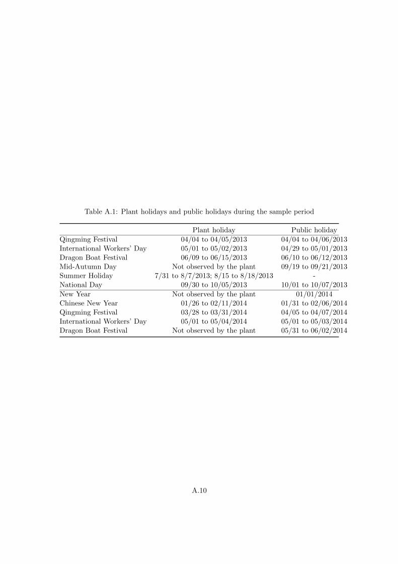
Table A.1: Plant holidays and public holidays during the sample period
Plant holiday Public holiday
Qingming Festival 04/04 to 04/05/2013 04/04 to 04/06/2013International Workers’ Day 05/01 to 05/02/2013 04/29 to 05/01/2013Dragon Boat Festival 06/09 to 06/15/2013 06/10 to 06/12/2013Mid-Autumn Day Not observed by the plant 09/19 to 09/21/2013Summer Holiday 7/31 to 8/7/2013; 8/15 to 8/18/2013 -National Day 09/30 to 10/05/2013 10/01 to 10/07/2013
New Year Not observed by the plant 01/01/2014Chinese New Year 01/26 to 02/11/2014 01/31 to 02/06/2014Qingming Festival 03/28 to 03/31/2014 04/05 to 04/07/2014International Workers’ Day 05/01 to 05/04/2014 05/01 to 05/03/2014Dragon Boat Festival Not observed by the plant 05/31 to 06/02/2014
A.10
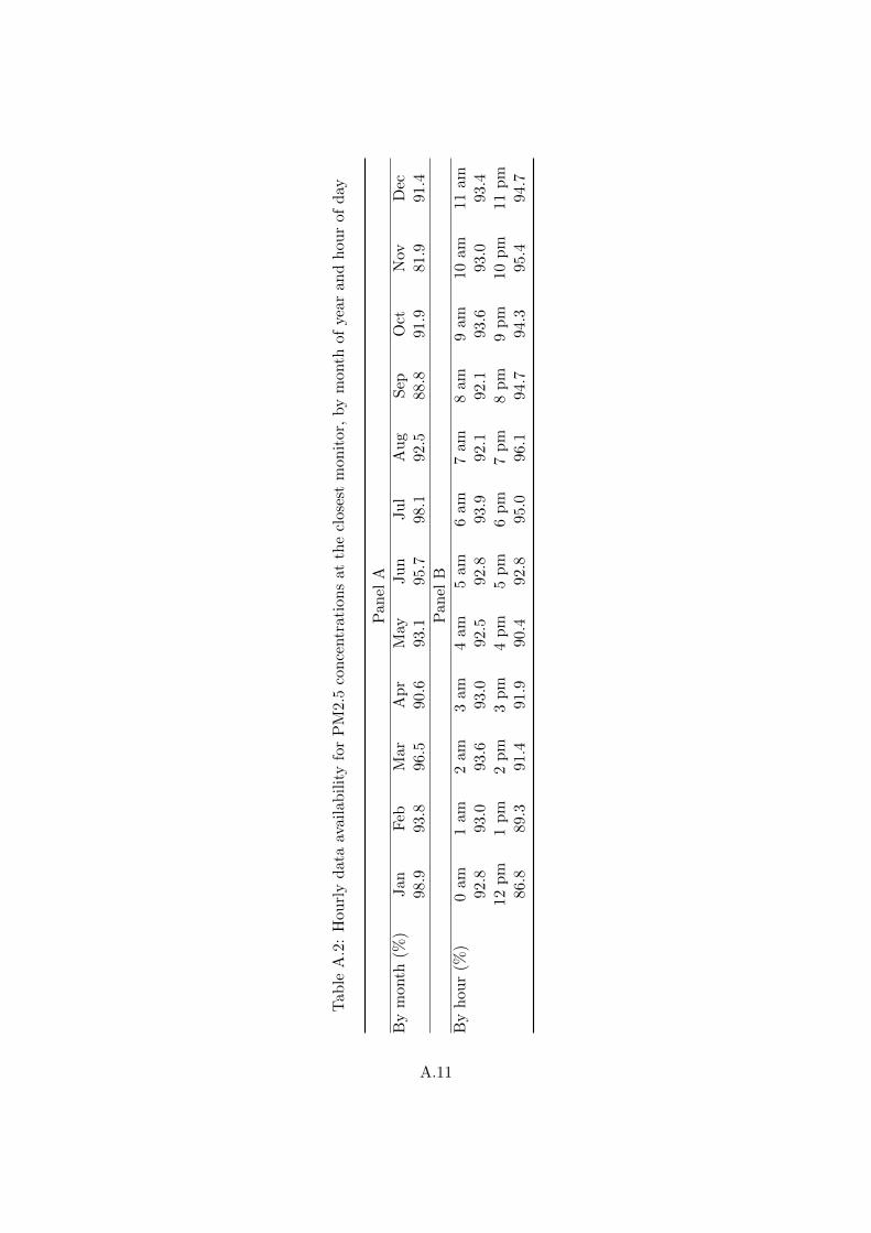
Tab
leA
.2:
Hou
rly
data
availab
ilit
yfo
rP
M2.
5co
nce
ntr
atio
ns
atth
ecl
oses
tm
onit
or,
by
mon
thof
year
and
hou
rof
day
Pan
elA
By
month
(%)
Jan
Feb
Mar
Ap
rM
ayJu
nJul
Au
gS
epO
ctN
ovD
ec98.
993.
896
.590
.693
.195
.798
.192
.588
.891
.981
.991
.4
Pan
elB
By
hou
r(%
)0
am1
am
2am
3am
4am
5am
6am
7am
8am
9am
10am
11am
92.
893.
093
.693
.092
.592
.893
.992
.192
.193
.693
.093
.412
pm
1p
m2
pm
3p
m4
pm
5p
m6
pm
7p
m8
pm
9p
m10
pm
11p
m86.
889.
391
.491
.990
.492
.895
.096
.194
.794
.395
.494
.7
A.11
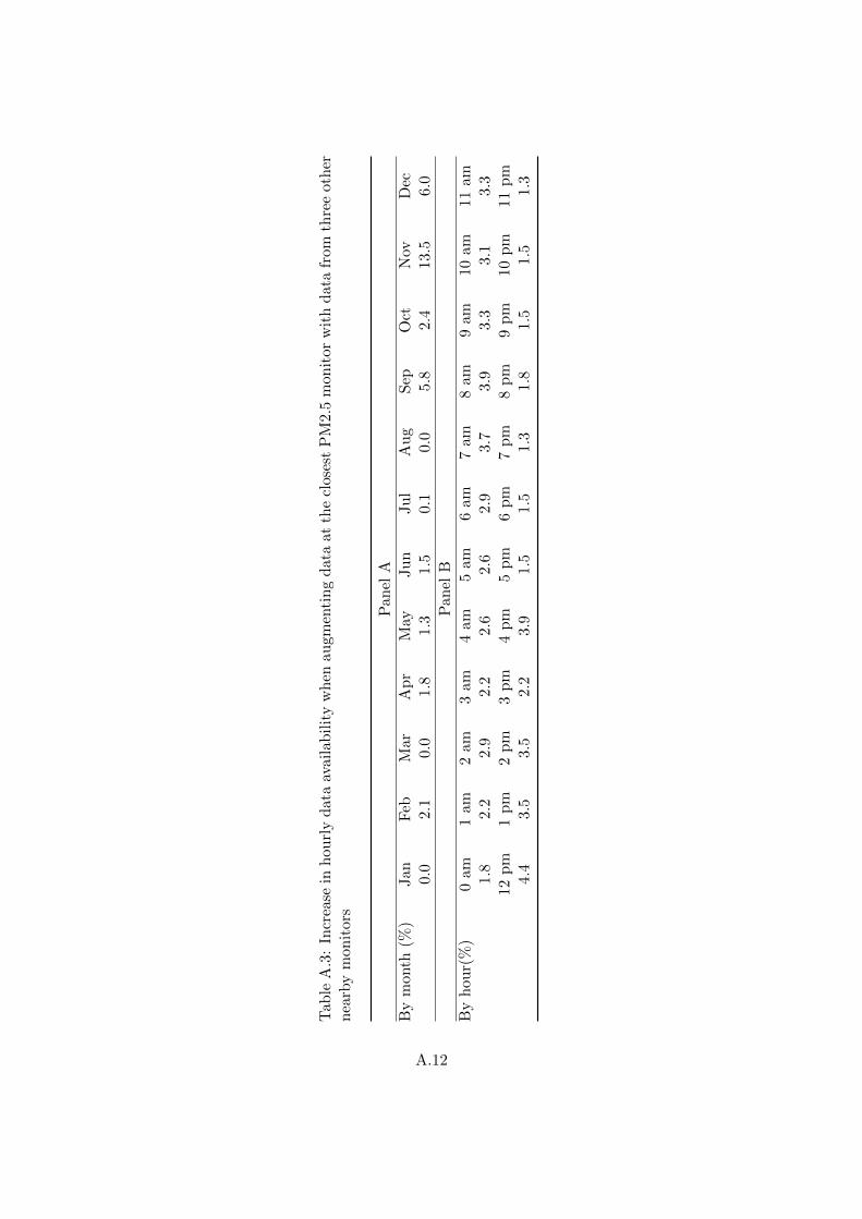
Tab
leA
.3:
Incr
ease
inh
ou
rly
data
avail
abil
ity
wh
enau
gmen
tin
gd
ata
atth
ecl
oses
tP
M2.
5m
onit
orw
ith
dat
afr
omth
ree
oth
ern
earb
ym
on
itors
Pan
elA
By
month
(%)
Jan
Feb
Mar
Ap
rM
ayJu
nJul
Au
gS
epO
ctN
ovD
ec0.
02.
10.0
1.8
1.3
1.5
0.1
0.0
5.8
2.4
13.5
6.0
Pan
elB
By
hou
r(%
)0
am
1am
2am
3am
4am
5am
6am
7am
8am
9am
10am
11am
1.8
2.2
2.9
2.2
2.6
2.6
2.9
3.7
3.9
3.3
3.1
3.3
12
pm
1p
m2
pm
3p
m4
pm
5p
m6
pm
7p
m8
pm
9p
m10
pm
11p
m4.
43.
53.5
2.2
3.9
1.5
1.5
1.3
1.8
1.5
1.5
1.3
A.12
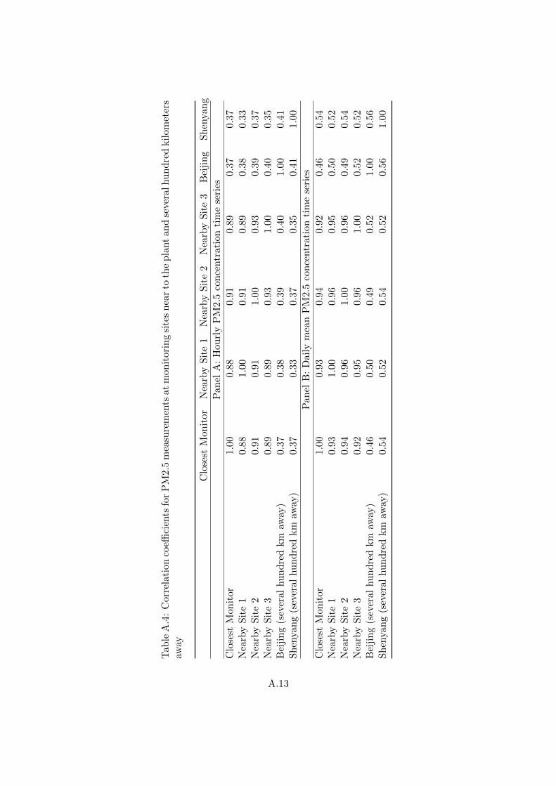
Tab
leA
.4:
Corr
elat
ion
coeffi
cien
tsfo
rP
M2.5
mea
sure
men
tsat
mon
itor
ing
site
sn
ear
toth
ep
lant
and
seve
ralhu
nd
red
kil
omet
ers
away
Clo
sest
Mon
itor
Nea
rby
Sit
e1
Nea
rby
Sit
e2
Nea
rby
Sit
e3
Bei
jin
gS
hen
yan
g
Pan
elA
:H
ourl
yP
M2.
5co
nce
ntr
atio
nti
me
seri
es
Clo
sest
Mon
itor
1.00
0.88
0.91
0.89
0.37
0.37
Nea
rby
Sit
e1
0.88
1.00
0.91
0.89
0.38
0.33
Nea
rby
Sit
e2
0.91
0.91
1.00
0.93
0.39
0.37
Nea
rby
Sit
e3
0.89
0.89
0.93
1.00
0.40
0.35
Bei
jin
g(s
ever
alhu
nd
red
km
away
)0.
370.
380.
390.
401.
000.
41S
hen
yan
g(s
ever
al
hu
nd
red
km
away
)0.
370.
330.
370.
350.
411.
00
Pan
elB
:D
aily
mea
nP
M2.
5co
nce
ntr
atio
nti
me
seri
es
Clo
sest
Mon
itor
1.00
0.93
0.94
0.92
0.46
0.54
Nea
rby
Sit
e1
0.93
1.00
0.96
0.95
0.50
0.52
Nea
rby
Sit
e2
0.94
0.96
1.00
0.96
0.49
0.54
Nea
rby
Sit
e3
0.92
0.95
0.96
1.00
0.52
0.52
Bei
jin
g(s
ever
alhu
nd
red
km
away
)0.
460.
500.
490.
521.
000.
56S
hen
yan
g(s
ever
al
hu
nd
red
km
away
)0.
540.
520.
540.
520.
561.
00
A.13
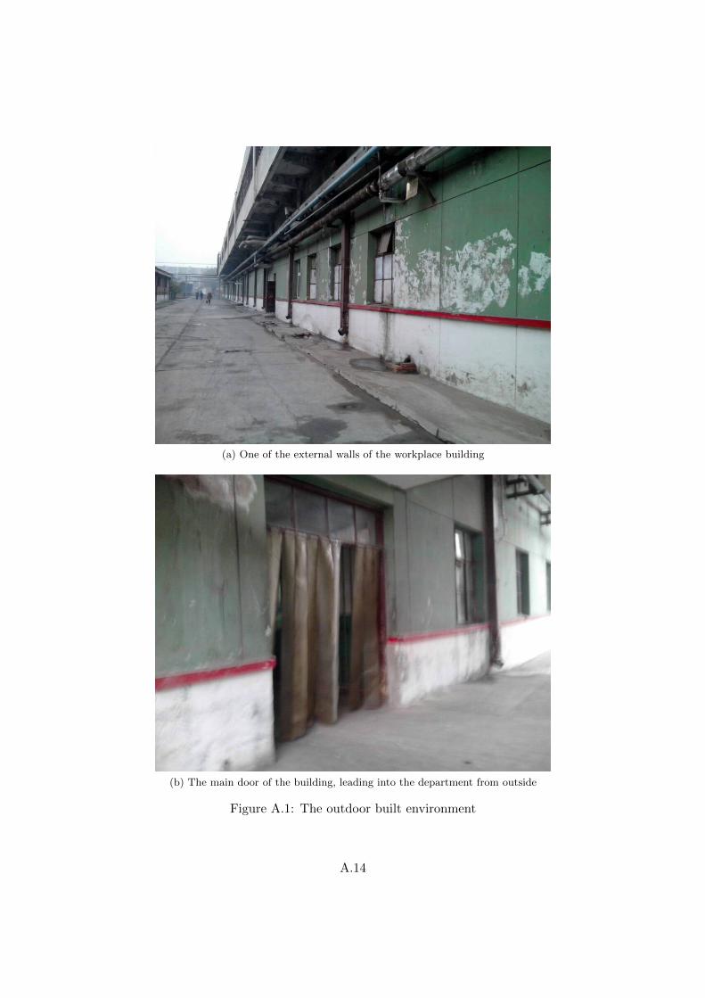
(a) One of the external walls of the workplace building
(b) The main door of the building, leading into the department from outside
Figure A.1: The outdoor built environment
A.14
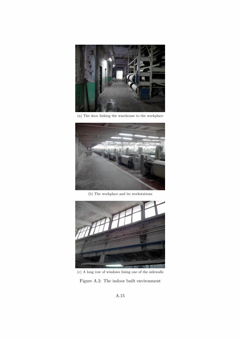
(a) The door linking the warehouse to the workplace
(b) The workplace and its workstations
(c) A long row of windows lining one of the sidewalls
Figure A.2: The indoor built environment
A.15
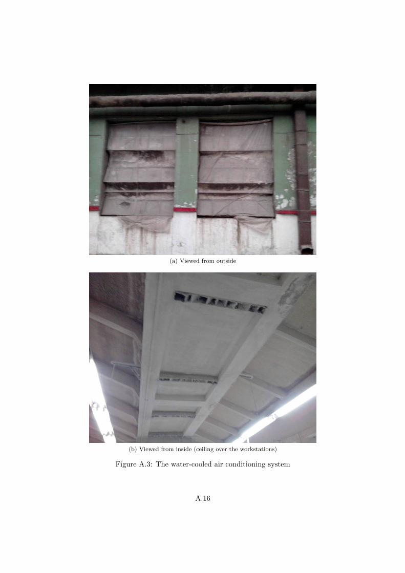
(a) Viewed from outside
(b) Viewed from inside (ceiling over the workstations)
Figure A.3: The water-cooled air conditioning system
A.16
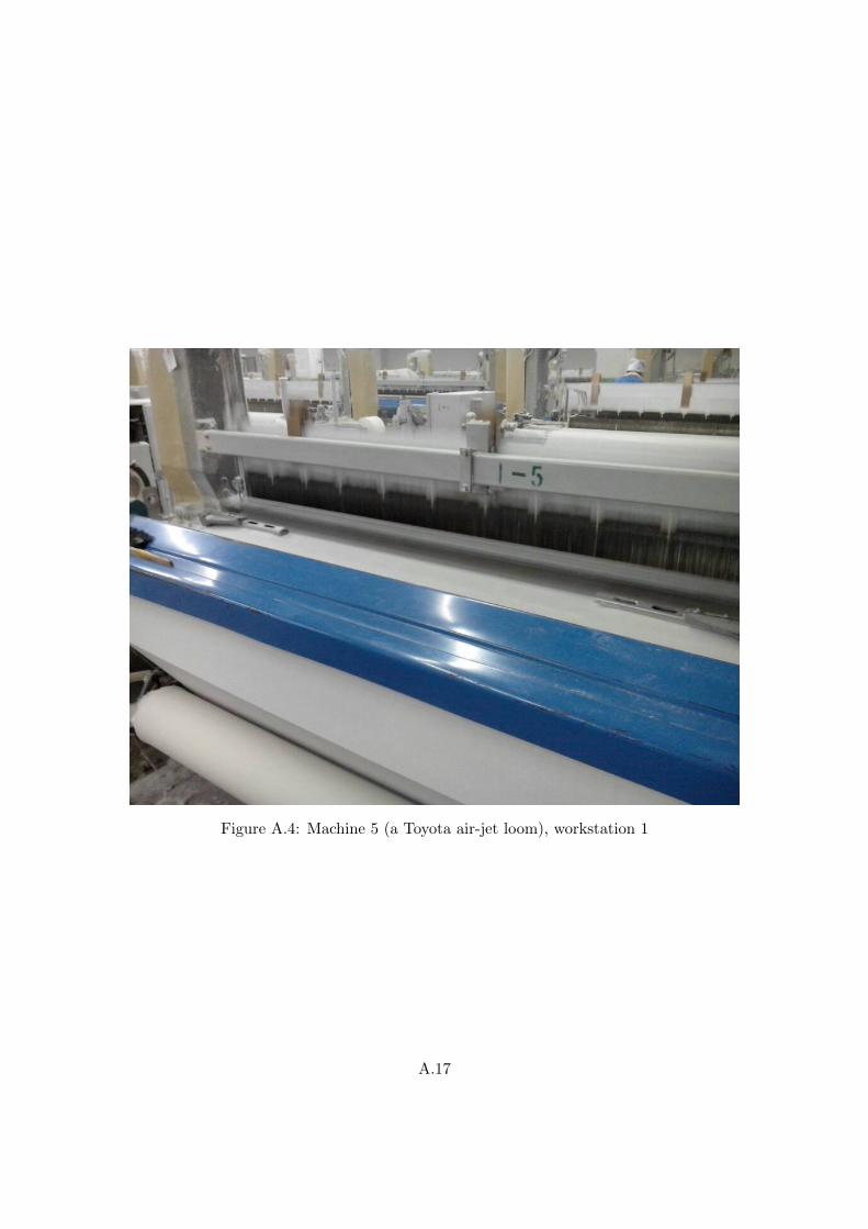
Figure A.4: Machine 5 (a Toyota air-jet loom), workstation 1
A.17
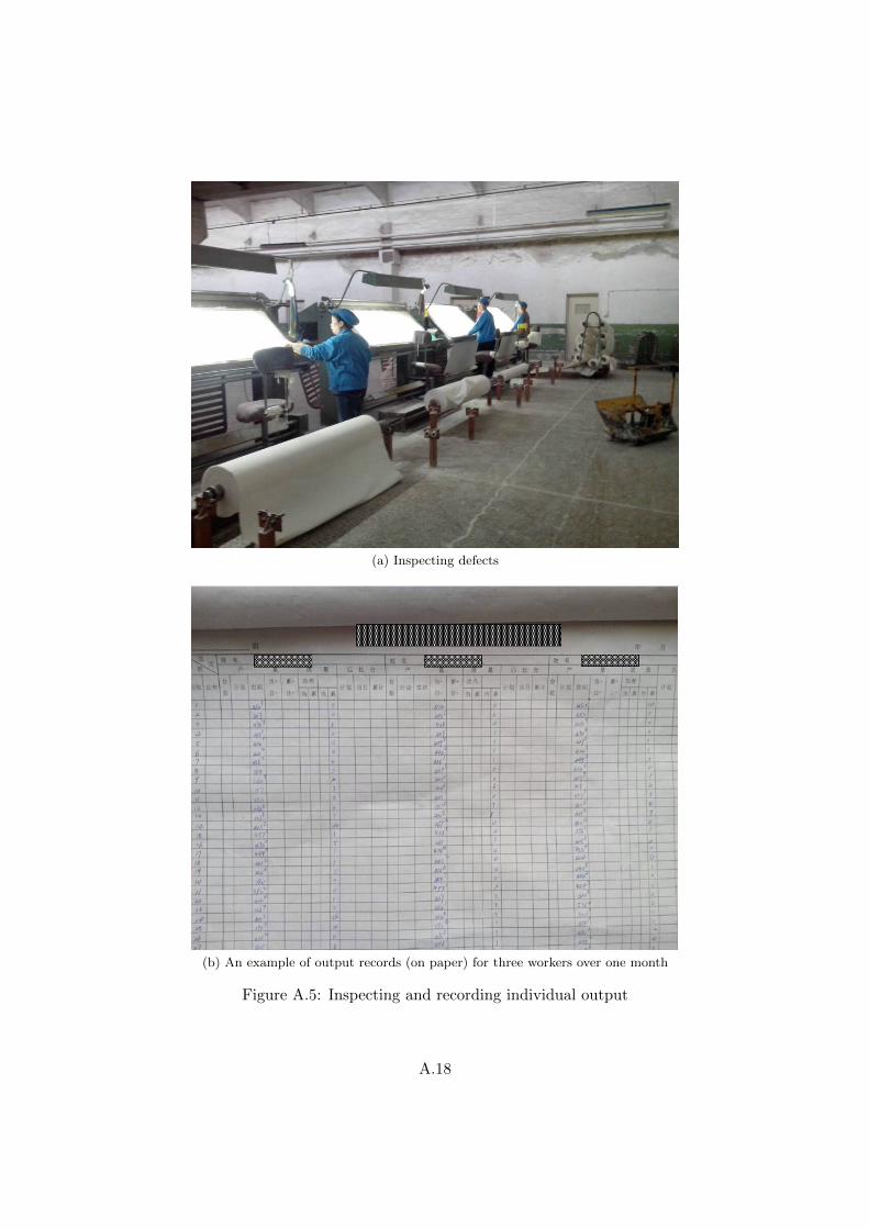
(a) Inspecting defects
(b) An example of output records (on paper) for three workers over one month
Figure A.5: Inspecting and recording individual output
A.18
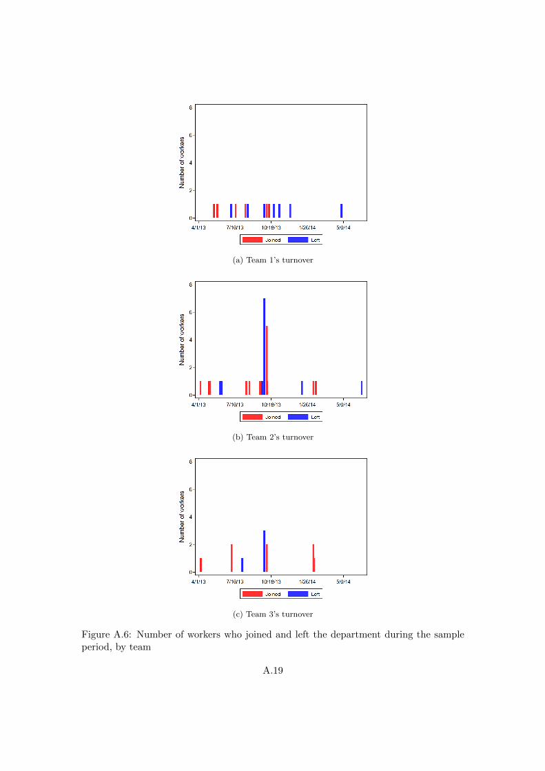
(a) Team 1’s turnover
(b) Team 2’s turnover
(c) Team 3’s turnover
Figure A.6: Number of workers who joined and left the department during the sampleperiod, by team
A.19
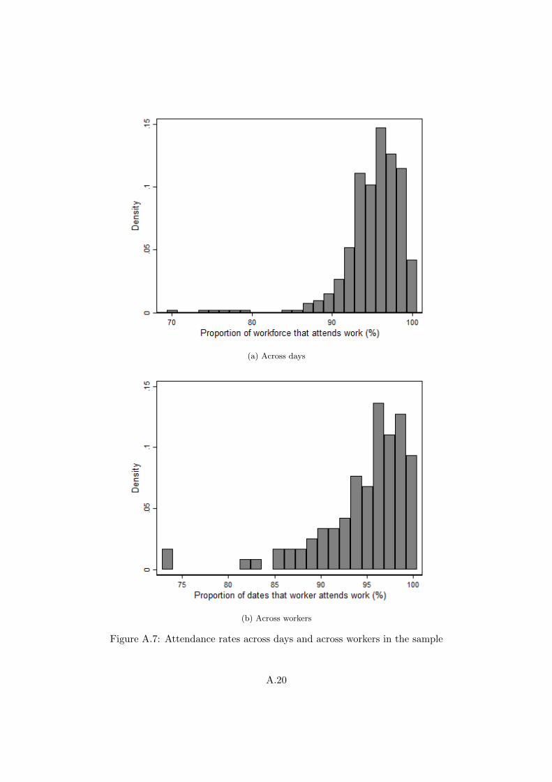
(a) Across days
(b) Across workers
Figure A.7: Attendance rates across days and across workers in the sample
A.20
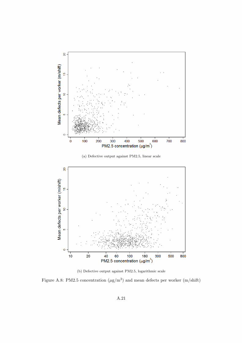
(a) Defective output against PM2.5, linear scale
(b) Defective output against PM2.5, logarithmic scale
Figure A.8: PM2.5 concentration (µg/m3) and mean defects per worker (m/shift)
A.21
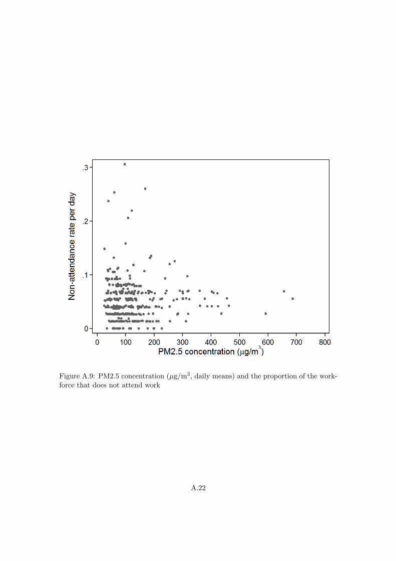
Figure A.9: PM2.5 concentration (µg/m3, daily means) and the proportion of the work-force that does not attend work
A.22
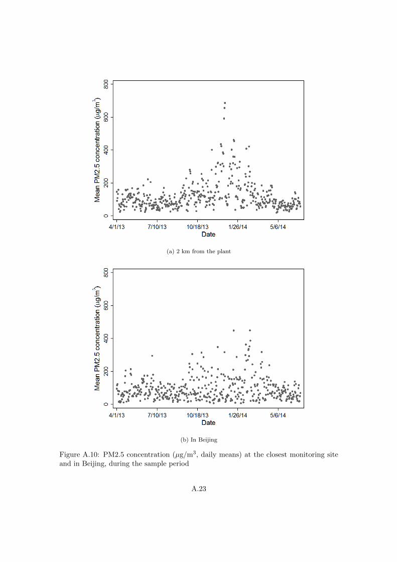
(a) 2 km from the plant
(b) In Beijing
Figure A.10: PM2.5 concentration (µg/m3, daily means) at the closest monitoring siteand in Beijing, during the sample period
A.23
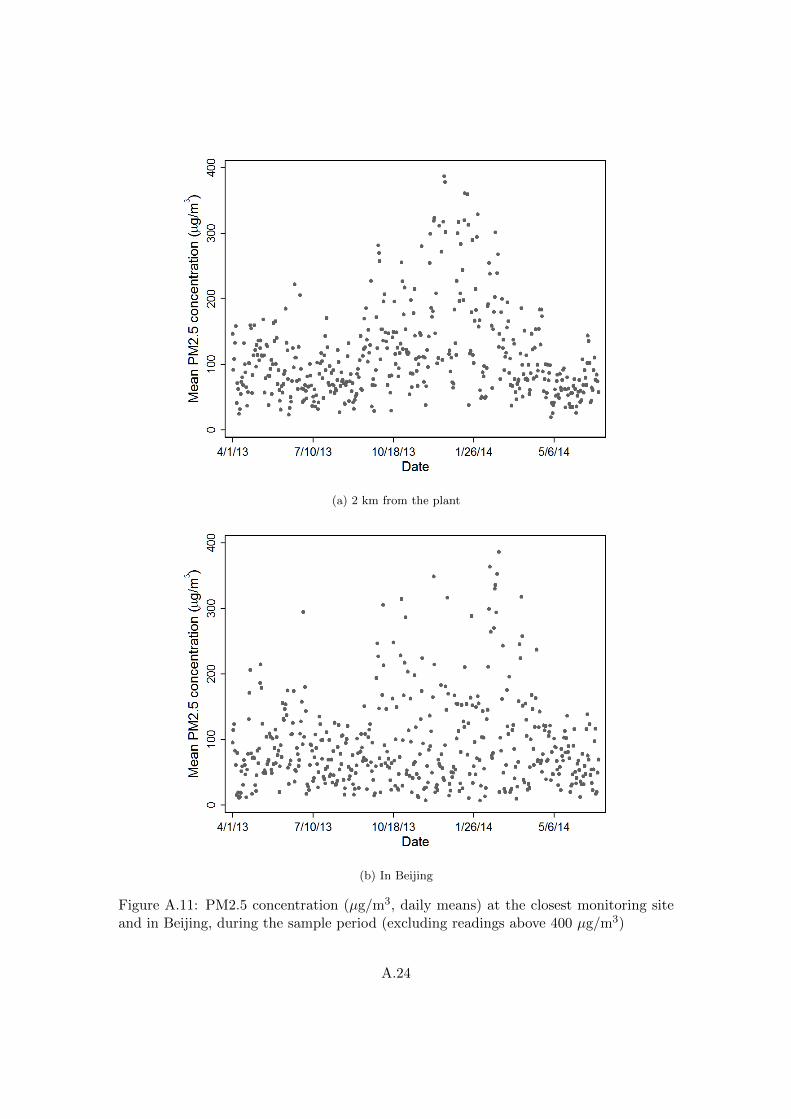
(a) 2 km from the plant
(b) In Beijing
Figure A.11: PM2.5 concentration (µg/m3, daily means) at the closest monitoring siteand in Beijing, during the sample period (excluding readings above 400 µg/m3)
A.24
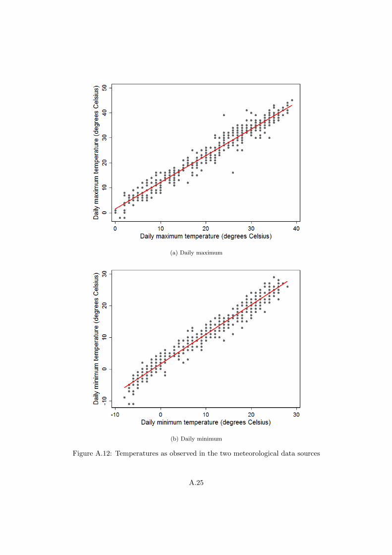
(a) Daily maximum
(b) Daily minimum
Figure A.12: Temperatures as observed in the two meteorological data sources
A.25
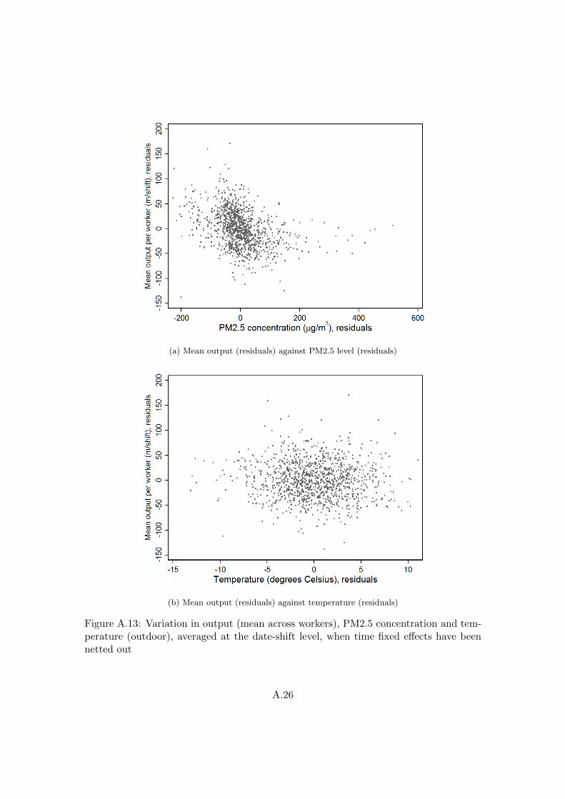
(a) Mean output (residuals) against PM2.5 level (residuals)
(b) Mean output (residuals) against temperature (residuals)
Figure A.13: Variation in output (mean across workers), PM2.5 concentration and tem-perature (outdoor), averaged at the date-shift level, when time fixed effects have beennetted out
A.26
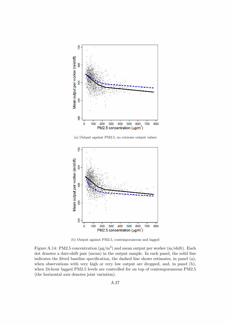
(a) Output against PM2.5, no extreme output values
(b) Output against PM2.5, contemporaneous and lagged
Figure A.14: PM2.5 concentration (µg/m3) and mean output per worker (m/shift). Eachdot denotes a date-shift pair (mean) in the output sample. In each panel, the solid lineindicates the fitted baseline specification, the dashed line shows estimates, in panel (a),when observations with very high or very low output are dropped, and, in panel (b),when 24-hour lagged PM2.5 levels are controlled for on top of contemporaneous PM2.5(the horizontal axis denotes joint variation).
A.27
Recommended


![Epidemiological estimates of Respiratory diseases in the ......Outdoor air pollution also causes severe respiratory diseases [11]. Outdoor air pollution is also one of the risk factor](https://img.pdfslide.us/doc/110x75/60780c853870e62a931c59c6/epidemiological-estimates-of-respiratory-diseases-in-the-outdoor-air-pollution.jpg)