Service Oligopolies and Australia’s Economy-Wide Performance*
Rod Tyers College of Business and Economics
Australian National University
Lucy Rees** Bain and Company
Key words: Regulation, oligopoly, services, price caps, privatisation
JEL codes:
C68, D43, D58, L13, L43, L51, L80
For presentation a the 11th Annual Conference on Global Economic Analysis Helsinki, 12-14 June 2008
* Funding for the research described in this paper is from Australian Research Council Discovery Grant No. DP0557885. Thanks are due to Flavio Menezes for valuable input at the formation stage of this project, Chris Jones for useful discussions, Marcin Pracz for assistance with this research during 2006 and to Pingkun Hsu and Iain Bain for research assistance since then. Flavio Menezes also offered valuable comments on an earlier draft as did participants at a March 2008 seminar in the ANU’s College of Business and Economics, including Phillipa Dee, Ben Smith, Chris Jones, Martin Richardson, William Coleman and Richard Cornes. ** Lucy Rees contributed to the early development of this research during her studies at the ANU. The results presented and opinions offered in no way represent the positions of Bain and Company on regulation policy.
2
Service Oligopolies and Australia’s Economy-Wide Performance Abstract
The retreat from public ownership of service firms and industries has left behind numerous private monopolies and oligopolies supervised by regulatory agencies. Services industries in government and private ownership generate two-thirds of Australia’s value added and employ three quarters of its workforce. This study offers an economy-wide approach that represents monopoly and oligopoly behaviour explicitly. It examines the implications of oligopoly rents for factor markets and the real exchange rate, the extent of sectoral interactions and the potential economy wide gains from tighter price cap regulation, with the results confirming the merit of an economy-wide approach. External shocks, like the present “China boom”, are also simulated. Such positive shocks are shown to expand the potential for oligopoly rents and therefore to raise the bar for regulatory agencies. Moreover, less than tight price caps are shown to exacerbate entry-exit hysteresis in boom and bust cycles. 1. Introduction
Following microeconomic reforms of the 1980s and 1990s, industries subject to
regulation now provide three quarters of Australian’s employment and two thirds of its GDP.1
The analysis of regulatory regimes must, therefore, account for economy-wide implications,
such as effects on the real exchange rate and factor markets as well as on other industries
through the cost of intermediate services. This requires the development of a model of the
whole Australian economy that incorporates explicitly the monopoly and oligopoly behaviour
requiring regulation in the first place. Such a model is offered in this paper. It is designed to
help clarify the implications of changes in the regulation of oligopoly pricing for the structure
and performance of Australia’s service industries while at the same time examining inter-
sectoral effects and associated changes in the performance of labour markets and the economy
as a whole.
The retreat from the government’s direct provision of infrastructure services has left
private firms and publicly-owned corporatised entities (government bodies subject to
corporations’ law) in industries that are littered with oligopoly structures and component
monopolies. These firms and entities are therefore supervised by regulatory agencies. Half of
their output originates in sectors whose ownership and regulatory structure has changed
substantially in the last decade. Most particularly, these sectors include: transport, electricity,
water supply and gas distribution, telecommunications, finance and insurance, education and
1 See ABS 2003: Tables 21.2 and 21.3.
3
health.2 While regulatory policies cover both product pricing and quality, we focus entirely
on price regulation, including price surveillance as well as price caps, and hence the control of
economic costs associated with distortions due to imperfect competition.
Some existing studies suggest an indirect link between the privatisation and regulatory
reforms and productivity3, while other studies follow a long tradition in regulatory economics
of applying industry-specific comparative statics.4 In recent years economy-wide
implications have been sought, though via models underpinned by perfectly competitive
behaviour, with oligopoly rents implied by the choice of parameters, closure or productivity
shocks.5 Industry-specific fix-ups in such models still require the assumption of perfect
competition in all other industries to generate the economy-wide effects. While this approach
has been very useful during the microeconomic reform transition, it tends to ignore the fact
that most other economic activity is also imperfectly competitive and subject to regulation,
and that regulatory changes to one industry are unlikely to occur without implications for the
regulation of others or for the performance of the whole economy.6
Central to this paper is the mathematical model of the Australian economy it
introduces and the economy wide database that serves it. This model represents monopoly
and oligopoly pricing behaviour and the regulatory environments facing major firms. Its
behavioural structure is based on early work by Harris (1984), Horridge (1987), Gunasekera
and Tyers (1990) and Tyers (2005), which emphasised homogeneous product oligopolies with
firms interacting on production in an “almost small” home economy. Subsequent extensions
included differentiated product oligopolies interacting on prices.7 The focus in these prior
applications has been trade reform and manufacturing oligopoly, wherein considerable
attention has been given to the “pro-competitive” effects of trade liberalisation (Hertel 1994;
Ianchovichina et al. 2000; Tyers 2005).
In its new guise the model is structured to focus on the more commonly regulated
services industries, following Rees (2004). To this end, a more complete representation of the
2 The health sector is not addressed independently in this study, primarily because its activity is difficult to distinguish in the available economy-wide database we use but also because it is rife with information asymmetries that make its regulation more complex than the sectors considered. 3 See, for example, Productivity Commission (1999). 4 Classic partial equilibrium studies include those by Averch and Johnson (1962), Courville (1974) and Wellisz (1963). 5 The best of these uses the well-constructed and highly detailed MONASH model of the Australian economy (Dixon and Rimmer 2002). Ours is not an attempt to compete with this model, or to come near its impressive attention to sectoral detail. Rather, we seek to construct a more direct means to evaluate regulatory policies by embedding more realistic monopoly and oligopoly behaviour in the economy-wide context. 6 This is notwithstanding the fact that regulation can be applied differently across different jurisdictions in Australia and across different industries. See, for example, NECG (2003). 7 For the antecedents of the approach adopted, see Golley (1993) and Tyers (2004).
4
Australian tax system is incorporated. This is needed for two reasons. First, the response of
firms to regulation depends on the rates of tax to which they are subject, and second, taxes
and transfers offer an alternative approach to the achievement of regulatory objectives.
Further, the model includes generic foreign ownership, thereby allowing for proper
representation of net factor income flows and their effects on the real exchange rate, the
composition of the current account and GNP.
Using this machinery, this paper begins with an assessment of the scale of costs the
Australian economy would bear were its oligopolistic service industries to be allowed to
cartelise. This hypothetical experiment is used to illustrate the extent of economy wide
interactions associated with oligopoly behaviour. It then assesses the potential for further
gains from tighter capping of prices, once again giving emphasis to economy wide
interactions. Finally, it offers a stylised representation of the Australian economy’s response
to the recent “China driven” global commodity boom, which directly affects its agricultural
and mining sectors but which has raised the relative prices of Australian services and so it has
important implications for oligopoly rents in services and their regulation. Indeed, the results
show that the maintenance of tight price caps through the boom would measurably increase
the benefit from it in the short run and avoid excessive entry in the long run should the effects
of the boom be transitory.
The section to follow briefly reviews developments in the structure and regulation of
Australia’s services sector. Section 3 reviews the behavioural structure of the model used, the
detailed description of which is consigned to appendices, and the economic structure
embodied in its database. The potential economic losses from oligopoly behaviour are
assessed in Section 4 while the gains to be derived from tighter price capping are considered
in Section 5. The response of oligopolistic services to external shocks is examined in Section
6, along with the effects of protection that could be called for in response. Conclusions and
priorities for further research are discussed in Section 7.
2. Regulation Research and Australia’s Services
Australia’s service industries have experienced rapid growth over the last fifty years.
Their regulation is seen as redress for market failures that include lack of information,
monopoly power, externalities or social objectives (income distribution or service quality).8
Many service industries require networks with hubs that constitute substantial recurrent fixed
8 See Findlay (2000: 10).
5
cost and the control of which creates barriers to entry, conferring monopoly power.9 The
economic rationale for service regulation is therefore strong.
Stigler (1971) argued that the analysis of regulation should concentrate on three
important questions10: who will receive the benefits and who will bear the burden of
regulation, the form and nature of the regulatory intervention, and the effect of regulation on
resource allocation. There is a very substantial subsequent literature on the positive aspects of
regulation. That detailing the specific regulations imposed on Australia’s services is vast and
complicated.11 Forms adopted range between price controls, ownership restrictions, limits on
foreign direct investment and capacity constraints. Federal responsibility for competition
regulation and monitoring rests with the Australian Competition and Consumer Commission
(ACCC), which administers the Trade Practices Act 1974 (“TPA”) and the Prices
Surveillance Act 1983 (“PSA”). The TPA promotes competition and fair trading while also
providing consumer protection. The PSA circumscribes the ACCC’s monitoring of prices,
costs and profits.12
The reach of regulatory policies in Australia has risen since these Acts were written,
due to the extensive privatisations associated with the “microeconomic reform” era and the
pace of technological change. The latter, particularly in telecommunications, electricity and
gas, has made it possible to “unbundle” industry segments, leaving some as natural
monopolies or oligopolies but with others organised around supervised new markets that
foster competitive behaviour (such electricity production and the retailing of gas, electricity
and telephone services). The introduction of price caps as “incentive regulation” was aimed
at the monopoly and oligopoly elements, where competitive pricing could not be otherwise
induced. These consequences of privatisation did, however, distort behaviour as investment
sought to escape the price caps.13 In telecommunications, air transport and the production and
distribution of natural gas and electricity these changes have been stark.14 Inevitable
distortions notwithstanding, these reforms have been shown to contribute to improvements in
both economic and government performance, according to the OECD (1997) to the tune of
five percent of GDP.
9 Ibid. In the Australian context a recent example of anti-competitive behaviour attributed to monopoly power over a network is Telstra’s pricing for its broadband service. See ACCC (2003). 10 See Stigler (1971). 11 See Trade Practices Act 1974 (Cth), reviewed in Productivity Commission (2003). 12 See ACCC (2003). 13 We are grateful to Flavio Menezes for this point. For related discussion, see Menezes et al. (2006). 14 See Doove et al. (2001: 43).
6
In the late 1970s there was significant anti-regulatory sentiment in developed
countries. The practice of rate-of-return regulation was found to be incompatible with
increased competition. Littlechild (1983) changed this negative perception of regulation with
his report on the British telecommunications industry in which he suggested price caps as a
regulatory policy tool. This signalled a movement towards a more incentive-based and less
heavy handed approach to regulation. The result has been very widespread application of
price-caps in services, which are characterised by: product-specific price ceilings, basket
ceilings that offer firms greater flexibility, and periodic adjustments of ceilings to ensure that
consumers share in the gains from technical change and market formation.15
Theoretical studies have been highly stylised and sector-specific but they demonstrate
that price-caps, even as second best measures, can protect consumers against monopoly
power, promote competition, improve productive efficiency and innovation and reduce the
administrative burden of regulation.16 Empirical follow-up by Xavier (1995) assesses price-
cap schemes in the UK, the USA and Australia. His Australian focus is on the (then)
Telecom basket price cap between 1989 and 1992. He finds that the scheme reduced the
average price of Telecom’s domestic services in real terms by 13 percent. International call
prices fell in real terms by 25 percent in this period, however, suggesting that the scheme fell
short of delivering a fair share of technological gains to the Australian consumer. He takes a
sceptical view of some price-cap mechanisms, preferring the fostering of competitive forces
where this is possible.
Turning to economy-wide approaches, Blanchard and Giavazzi (2003) offer an
elemental general equilibrium model to investigate the combined effects of product market
and labour market regulation. Their closed economy model incorporates monopolistic
competition in the goods market and bargaining in the single factor (labour) market. In
seeking competition, a government might try to raise the elasticity of substitution. In the
short-run they find that the increased competition is beneficial because it forces firms to lower
their mark-up, leading in turn to reduced capital returns but a higher real wage. In the long
run, however, there is exit by firms and reduced product variety. The assumption of
monopolistic competition leaves no pure profits to erode and invariant recurrent fixed costs
must see the mark-up return to its original value, so there are no long run benefits. If, instead,
the government attacks barriers to entry (recurrent fixed costs), the effects are unambiguously
welfare improving in the short and long runs. There is an increase in the number of firms, a
15 See Vogelsang and Acton (1989). 16 The key works in this area are: Cabral and Riordan (1989), Bradley and Price (1988), and Brennan (1989).

7
higher elasticity of demand, a lower mark-up and thus lower unemployment and a higher real
wage. While it is not made clear how a government might alter the elasticity of substitution
or entry costs, this research signals an improvement over prior studies of regulation through
its characterisation of market structure in an economy-wide context and it is in this spirit that
the research presented in this paper has been undertaken.
The precise extent of imperfect competition in Australia’s service industries is
difficult to quantify. We offer short qualitative summaries for the key sectors in which
privatisation and regulation have brought most change.
Telecommunications
The ACCC’s analysis indicates that this sector is slowly becoming more competitive,
with most improvement at the retail level, as opposed to infrastructure provision. Telstra
continues to be the dominant firm with about two thirds of the sector’s listed market
capitalisation and between a third and three quarters of the markets for the different
telecommunications products (Telstra 2003). While these facts suggest a high level of
concentration, in areas such as mobile and long distance telephony and data transfer,
competition is intense. Telstra’s exploitable market power is in fixed telephony and network
access.17
Electricity
New market mechanisms as well as regulatory reform have been introduced in this sector. It
has nonetheless been found that generators, whose numbers remain small, have often been
able to increase prices substantially above competitive levels for sustained periods. Indeed,
Short et al. (2001) indicate that the electricity market is subject to significant departures from
competitive outcomes. High Lerner indices (price-marginal cost margins) suggest the
collection of substantial rents. Yet, given this industry’s high fixed costs, a better measure
might have been the mark-up over average cost.
Gas
While official barriers to the free flow of natural gas across state borders have been removed,
the market remains highly concentrated on the supply side and it carries many legacy
agreements that limit competition. The resulting lack of liquidity in Australian gas markets
17 For this point we are grateful to Flavio Menezes.
8
has impeded the development of transparent spot markets.18 There are three suppliers in the
eastern Australian gas markets that account for more than 95 percent of the supply gas. The
two incumbents BHP Billiton and ExxonMobil account for 38 percent and 41 percent
respectively. As to infrastructure, the largest pipeline owner in Australia is Australian
Pipeline Trust (APT) which owns a third of the total transmission pipeline system.19
Australia’s second largest pipeline owner is Epic Energy, with about half the capacity of APT.
In 1997 the Australian Government introduced a Gas Code – The National Third Party Access
Code for Natural Gas Pipelines – which is administered by the ACCC and the National
Competition Council (NCC).20 The Code ensures that gas can be transmitted through the
pipeline network on ‘reasonable’ terms and conditions, though in practice these have attracted
controversy.
Air Transport
The Australian airline domestic market has long had a duopoly structure, changes of
players in the 1990s notwithstanding. Because of volatility associated with these changes, the
market share of the only remaining incumbent, Qantas, has been measured at and above 70
percent.21 Nonetheless it remains in the interest of both the major carriers to maintain an
industry structure which allows both to generate sustainable profitability without encouraging
further entry. Again, the ACCC monitors prices and frequent flyer schemes for anti-
competitive elements. As to aviation infrastructure, prior to 2002, airports in Australia were
subject to price-cap regulation. However, the Productivity Commission concluded that while
the major metropolitan airports have substantial market power, it is not in their interests to
abuse this power in such a way that would confer large costs onto the economy.22 Hence, the
government has largely deregulated airports, replacing price caps with price monitoring.23
Debate continues, however, as new air service entrants seek access to airport services.
This very brief review makes it clear that the regulation of oligopoly service industries
in Australia is made more complex by the trend toward the subdivision of each industry into
more and less competitive components. In this paper, however, our purpose is to take a broad
brush to the estimation of economy wide effects of service oligopoly behaviour. We therefore
18 See Short, C. et al. (2003). 19 See Australia Daily (2004). 20 See Moran (2002). 21 See Freed (2004). 22 See Productivity Commission (2002). 23 Rather than collude to raise carrier costs, owners of privatised airports have sought and found profitability through the development of airport property by exploiting relatively relaxed federal regulations governing the use of airport land.
9
work at the level of 10 sectors, necessarily averaging out sectoral detail. In interpreting the
research that follows it should be borne in mind that the task of sectoral regulators is not only
made difficult by the non-transparency of the costs we model but also because product lines
and the degree of differentiation between firms are not stable through time in the way we
model them.
3. An Oligopoly Model of the Australian Economy
The model is a development of that used to examine pro-competitiveness effects of
trade liberalisation in manufacturing by Tyers (2004, 2005).24 The version described here
differs in five key respects. First, behavioural equations have been added to represent the
effects of regulatory policy, including Ramsey price-caps; second, a government sector has
been included to distinguish the government’s expenditures from those of the collective
household. Previously, net revenue from border taxes was transferred to the collective
household in lump-sum. Like the model’s single private household, the government now has
Cobb-Douglas preferences over goods and a constant elasticity of substitution (CES) sub-
aggregation of home goods with imports. It is not, however, treated as an optimising agent
maximising a utility function like the representative household.25 A balanced budget is
assumed so that government spending changes in line with tax revenue.
Third, the border tax system in the earlier version of the model has been extended to
include a more detailed representation of Australia’s tax system with both direct (income)
taxes levied separately on labour and capital income and indirect taxes including those on
consumption, imports and exports.26 Fourth, a new database is constructed that emphasises
Australia’s service industries. This database incorporates government consumption and the
complete tax system.27 Fifth and finally, stability problems encountered in the tradable goods
sectors due to a uniform structure suited to the more closed services sectors necessitated a
restructuring of the model’s treatment of foreign goods. These are now considered
24 It is a distant descendent of the models of Harris (1984) and Gunasekera and Tyers (1990). 25 One approach, not adopted in this paper, would be to incorporate the government sector so that its spending and taxation decisions are endogenous and determined by the maximisation of an assumed social welfare function. The difficulty with such an approach is that it does not capture the political economy of government policy. Thanks are due to Chris Jones for useful discussions on this topic. 26 Income taxes are approximated by flat rates deduced as the quotient of revenue and the tax base in each case. 27 These first four advances are due to Rees (2004).
10
homogeneous in each broad sector but differentiated from corresponding home products,
which themselves are differentiated by variety.28
Model structure
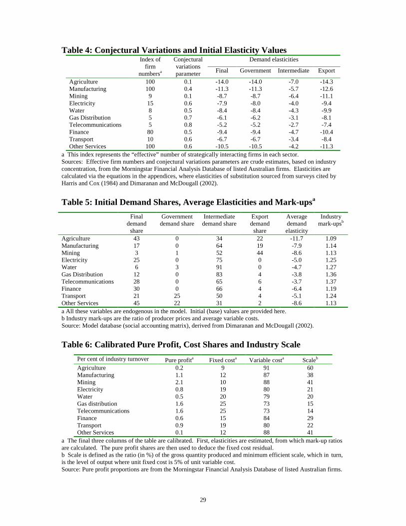
The scope of the model is defined in Table 1. It divides the Australian economy into
ten sectors, of which seven offer services, and four primary factors. The ten sectors are
chosen to reflect the dominance of services in domestic demand and the importance of
regulation to imperfectly competitive services sectors. Firms in all ten sectors are
oligopolistic in their product pricing behaviour with the degree of price-setting collusion
between firms represented by conjectural variations parameters. The magnitudes of these
parameters are considered to represent the flexibility allowed the firms pricing behaviour by
the surveillance of regulatory agencies. Each firm bears fixed capital and skilled labour costs,
enabling the representation of unrealised economies of scale. Home products in each sector
are differentiated by variety29 and output is Cobb-Douglas in variable factors and intermediate
inputs. Intermediate input demands are CES subaggregates of home and imported products.
Despite their oligopoly power in product markets, firms have no oligopsony power in the
markets for primary factors or intermediate inputs. The sophistication with which home
product markets are represented notwithstanding, the modelling of a single economy
necessitates crudeness in the representation of foreign firms. Thus, imports are seen as
homogeneous, differentiated from home products as a group, so that import varietal diversity
never changes.30
In the long run, physical capital is homogeneous and fully mobile between sectors and
internationally, while the domestic endowments of other factors are fixed. A short run closure
is also constructed, wherein capital use in each industry is fixed and rates of return on capital
can vary between sectors. In this version, the closure can be adjusted correspondingly, so that
the real wage of unskilled labour is fixed and unskilled employment is endogenous. The
quantity of domestically-owned capital is fixed both in the short and long runs, so that
changes in the total capital stock affect the foreign ownership share and hence the level of
28 The earlier version required very large elasticities of substitution between varieties, leading to unrealistic behaviour in response to changes in border tariffs. Moreover, in a single economy model there is no satisfactory way to endogenise the number of foreign product varieties. 29 Product differentiation is assumed to be of the Spence-Dixit-Stiglitz type. This means that each individual derives utility from consuming a number of varieties of a given product. 30 Since all home varieties are exported there is no movement on the “extensive margin” of the type that is evident in the models of non-homogeneous export sectors by Melitz(2003) and Balistreri et al. (2007). We see this as acceptable in this study because our focus is on largely non-traded services.
11
income repatriated abroad. The economic profits or losses earned by firms are dependent on
the closure, under which either the number of domestic firms (varieties) can be fixed while
profits are endogenous, or flexible while economic profits are fixed.
The economy modelled is “almost small”, implying that it has no power to influence
border prices of its imports but its exports are differentiated from competing products abroad
and hence face finite-elastic demand.31 The effective numeraire is the import product bundle,
since import prices are exogenous in all experiments. Its current account deficit (of about a
tenth of its initial GDP) is fixed in terms of foreign prices in all experiments.32 For
presentational purposes, prices and values can be divided through by the consumer price or
the GDP price index so that the initial consumption or production bundle becomes the
numeraire. The consumer price index is constructed as a composite Cobb-Douglas-CES
index of home product and after-tariff import prices, derived from the single household’s
expenditure function and measured after consumption taxes are applied. This formulation of
the CPI aids in the analysis of welfare impacts. Because collective utility is also defined as a
Cobb-Douglas combination of the volumes of consumption by product aggregate,
proportional changes in overall economic welfare correspond with those in real GNP.33
Firms in any sector supply differentiated products and interact on price. Cobb-
Douglas production drives variable costs so that average variable costs are constant if factor
and intermediate product prices do not change. Consequently, while ever factor and
intermediate product prices are constant, average total cost declines with output. The
magnitudes of recurrent fixed costs are calibrated from data on industry profitability, gross
31 This follows the practice in national modelling since the first significant economy-wide model by Dixon et al. (1982) and the first published economy-wide oligopoly model by Harris (1984). 32 This implies that the acquisition of Australian assets by foreigners remains constant irrespective of shocks imposed on the model and their consequences. 33 When the utility function is Cobb-Douglas in consumption volumes, the expenditure function is Cobb-Douglas in prices. If the consumer price level, CP , is defined as a Cobb-Douglas index of prices, the equivalent variation in income can be expressed in terms of the proportional change in this index. Thus, following any shock, the income equivalent of the resulting changes to income and prices is:
( )1 0 0 1 1 1 0 11
, ,C
C CC
PW Y Y EV P P Y Y Y Y
P
∆∆ = − + = − − ,
which can be expressed in proportional change form as:
1 01
0 0 1
1C
C C
C
PY Y
PW Y P
W Y Y P
∆− − ∆ ∆ ∆ = ≅ − .
This is, approximately, the proportional change in real GNP.
12
value of output and value added.34 Firms charge a mark-up over average variable cost so that
it is at least possible for them to cover their average fixed cost in a zero-pure-profit
monopolistic competition equilibrium. They choose this mark-up strategically, however, so
that their capacity to push their price beyond their average variable costs without being
undercut by existing competitors then determines the level of any pure profits and the
potential for entry by new firms. As intuition would suggest, under free entry pure profits are
eroded and the mark-up just covers average total costs.
Each firm in industry i is regarded as producing a unique variety of its product and it
faces a downward-sloping demand curve with elasticity εi (< 0). The optimal mark-up is then:
(1) 1
11
ii
i
i
pm i
vε
= = ∀+
,
where ip is the firm’s product price, iν is its average variable cost and iε is the elasticity of
demand it faces. Firms choose their optimal price by taking account of the price-setting
behaviour of other firms. A conjectural variations parameter in industry i is then defined as
the influence of any individual firm k, on the price of firm j:
(2) iji
ik
p
pµ
∂=
∂ .
These parameters are considered to indicate the power of price surveillance by such
institutions as the ACCC. The Nash equilibrium case is a non-collusive differentiated
Bertrand oligopoly in which each firm chooses its price, taking the prices of all other firms as
given. In this case the conjectural variations parameter (2) is zero. When firms behave as a
perfect cartel, it has the value unity. This parameter enters the analysis through the varietal
demand elasticity, which is formulated in Appendix 2.
To study the effects of price-caps a regulated Ramsey mark-up, Rim is formulated as:
(3) R i ii
i
afcm
νν
+= .
Firms are permitted to choose compromise mark-ups by altering the parameter iϕ in the
following:
(4) ( ) ( )1 2C Ri i i i im m m iϕ ϕ= − + − ∀ .
34 In the starting equilibrium it is assumed that each industry has pure profits equal to one percent of gross earnings. Consistent secondary data are not readily available to determine the share of pure profits in capital returns in all industries.
13
Thus, when 1 , Ci i im mϕ = = , and when 2 , C R
i i im mϕ = = .
Critical to the implications of imperfect competition in the model is that the product of
each industry has exposure to four different markets. It can be consumed by private
households or by government, used as an intermediate input in another industry or it can be
exported. The elasticity of demand faced by firms in industry i, εi, is therefore dependent on
the elasticities of demand in each of these four markets, as well as the shares of the home
product in each. More precisely, the four sources of demand for home produced products are
final demand (F), intermediate demand (I), export demand (X) and government demand (G).
For sector i, the elasticity sought is a composite of the elasticities of all four sources of
demand.
(5) ,F F I I X X G G
i i i i i i i is s s s iε ε ε ε ε= + + + ∀
where jis denotes the volume share of the home product in market i for each source of
demand j. These share parameters are fully endogenous in the model. Because the different
sources of demand are differently elastic, with export demand most elastic and intermediate
demand least, any shock that reapportions demand between them necessarily changes the
competitive behaviour of the firms.35 Almost all conceivable shocks do this to some degree.
Thus, the strategic behaviour of firms, and hence the economic cost of service
oligopolies, is affected by conjectural variations parameters as they represent collusive
capacity on the one hand and regulatory price surveillance on the other, and by the
composition of demand as it influences the elasticities of demand faced by each firm. Of
course, the capacity firms have to reduce their prices also depends on their productivity
performance, which we do not examine in this paper, and on their numbers, hence the sectoral
fixed cost burden.
The database and its representation of broad economic structure
The model database was constructed from the GTAP Version 5 global database for
1997 (Dimaranan and McDougall 2002).36 It combines detailed bilateral trade, transport and
protection data characterizing economic linkages among regions, together with individual
country national accounts, government accounts, balance of payments data and input-output
35 Export demand is found to be more elastic because of the larger number of substitutable product varieties available abroad while intermediate demand is relatively inelastic because of firms’ reluctance to alter arrangements for intermediate input supply which may depend on location or “just in time” relationships. These issues are addressed by Harris and Cox (1983). 36 Documentation on the GTAP 5 Data Package may be viewed at: <http://www.gtap.agecon.purdue.edu/databases/v5/v5_doco.asp>.

14
tables which enable the quantification of inter-sectoral flows within regions. From the
database key elements of our representation of the Australian economy emerge. From Table
2, it is evident that the privatised services, electricity, water, gas, telecommunications, finance
and transport, supply about a fifth of the economy’s GDP, yet their participation in
international trade is tiny compared with agriculture, manufacturing and mining. Moreover,
the privatised services are shown in Table 3 to be more intensive in skill and physical capital
than are the tradable sectors so that their comparative performance has particular implications
for the skilled wage premium and total capital use.
The flows represented in the database do not reveal details of sectoral structure. In
particular, additional information is required on firm numbers, pure profits, fixed costs and
minimum efficient scale for each sector. While some details are available on these variables
for some industries, there is no readily available source that is consistent and comparable
across sectors. With the support of the few industry studies already mentioned, these
variables are calibrated in the following manner. First, pure profits are required as a share of
total capital income (operating surplus) in each industry. This is needed to finalise the flow
database but also to calibrate industry competitive structure. For this we have resorted to data
on the profitability of listed firms from the Morningstar Financial Analysis Database.37
Second, rough estimates of strategically interacting firm numbers in each industry and
their corresponding conjectural variations parameters are required. It is not sufficient simply
to record the number of establishments in each industry, however. Unless industries are
subdivided finely, considerable diversity of firm size and product is embodied in each.
Indeed, within a particular industry classification, many firms supply intermediate inputs to
other firms in the same classification. Prices of the products that emerge from a particular
industry are very likely determined by a small proportion of the firms within it. Again, we
resort to the Morningstar database for measures of industry concentration. From this we
assign the crude index of firm numbers indicated in Table 4 and we also posit the
corresponding conjectural variations parameters shown in the same table.
Third, to complete the formulation of industry demand elasticities, elasticities of
substitution between home product varieties and between generic home and foreign products
are required for each sector. These are drawn from the estimation literature.38 Initial industry
37 After tax profits rates are compared with the prime borrowing rate in the period 1997-2007 to obtain measures of pure profits. Firm statistics were drawn from http://www.aspectfinancial.com.au/af/finhome?xtm-licensee=finanalysis.for and the data on industrial borrowing rates was from www.rba.gov.au. 38 Summaries of this literature are offered by Dimaranan and McDougall (2002) and at http://www.gtap. purdue.edu/databases/..
15
demand elasticities are then calculated for each source of demand (final, intermediate,
government and export), via the equations in the appendices, and the results are also listed in
Table 4. Initial shares of the demand facing each industry are then drawn from the database
to enable the calculation of a weighted average demand elasticity for each industry. Mark-up
ratios are then deduced from these, fixing average variable cost in each sector, via equation
(1). The initial equilibrium industry shares, average elasticities and mark-up ratios for each
sector are given in Table 5. Note that the elasticities appear large in magnitude at first glance.
This is because they do not represent the slopes of industry demand curves for generic goods.
Rather, they are the elasticities faced by suppliers of individual varieties and are made larger
by inter-varietal substitution.
This completes the demand side calibration. It enables us to turn to the calibration of
the supply side, where we begin by using the mark-up ratios to deduce the initial level of
average variable cost in each sector. Next, we turn to pure profits. The proportion these
make up of total turnover is deducted to arrive at fixed cost shares of total turnover.39 Total
recurrent fixed cost in each sector then follows. It is now possible to obtain a sense of the
scale of production.40 If industries could expand indefinitely without changing unit factor
rewards (the partial equilibrium assumption that is relaxed here), average fixed cost would
approach average variable cost asymptotically from above. Following Harris and Cox (1983)
we choose an arbitrary minimum efficient scale (MES) product volume at the point where
average fixed cost would decline to a twentieth of average variable cost. The results of this
calibration are summarised in Table 6. It confirms expectations that fixed costs are most
prominent in electricity, gas, water and telecommunications services, due to fixed physical
infrastructure and network maintenance costs. The results also suggest, plausibly, that the
sectors closest to their minimum efficient scale are agriculture, mining and “other services”.
4. Sectoral Interactions with Oligopoly
To explore the interdependence of the privatised service sectors and the potential
impacts of their non-competitive behaviour on the economy as a whole we begin by
considering the effects of complete exploitation of market power in all sectors. In particular,
on the presumption that oligopoly firms fail to collude and form cartels (or consolidate into
39 Fixed costs take the form of both physical and human capital costs using the rule of thumb (based on estimates by Harris and Cox, 1983) that physical capital has a fixed cost share of 5/6. 40 The actual calibration process is more complex than this because the elasticities of intermediate demand depend on intermediate cost shares, which depend on the variable cost share. It is therefore necessary to calibrate iteratively for consistency of elasticities and shares.
16
monopolies) mainly because of government price surveillance and (the threat of) anti-trust
actions,41 we imagine what the 1997 Australian economy would have looked like had these
government activities never occurred. A long run closure is selected in which physical capital
is internationally and intersectorally mobile and labour markets clear at flexible wages. The
entire economy is first allowed to cartelise, by raising all conjectural variations parameters to
unity.42 Then, individual sectors are cartelised one by one in a bid to identify non-linearities
that might imply the necessity of economy-wide analysis. The results of this exercise are
summarised in Table 7.43
Clearly the economy would have been substantially smaller if all sectors had been
cartelised. Real GDP would have been smaller by almost a quarter and real wages smaller by
almost half. Higher home relative to foreign prices imply an appreciated real exchange rate
and reduced trade with the rest of the world. If the cartelisation had only occurred in the
recently privatised services, electricity, water, gas, telecommunications, finance, transport and
“other services”, GDP would have been smaller by a tenth and real wages by a seventh. The
last decade or so has seen the avoidance of the latter outcome added to the responsibilities of
Australia’s regulatory institutions.
The central block in the table indicates how cartelisation by each individual sector
affects overall economic performance. It is clear that sectors like manufacturing and “other
services”, which have large initial shares of GDP, also have the largest impacts on the
economy following cartelisation. Since cartelisation implies reduced output and therefore
reduced factor and input demand, unit factor rewards fall in all cases. Some of the smaller
services sectors do have particularly large impacts on factor rewards, however, due to the
pattern of factor intensities indicated in Table 3.44 Average gross (of depreciation) rates of
return on capital include pure profits and, not surprisingly, are greatly boosted by
cartelisation. Only cartelisation of the manufacturing sector reduces this average gross rate of
return, and this is because manufactured inputs are extensively used in other sectors, the
41 This ignores the roles of contestability and the free rider problem in the maintenance of cartels. 42 The number of firms is held constant in this closure but it is, in any case, immaterial so far as pricing is concerned when industries are cartelised. Consolidation to a monopoly would reduce fixed costs and thereby increase monopoly profits, however, a development not explored here. 43 It stretches credibility to imagine that sectors with large numbers of small firms, such as agriculture, could overcome free rider and communication costs in this way. Taking agriculture as an example, however, the Australian sector is rife with organised “boards” designed to extract rents for farmers (Sieper, 1982). Even the “other services” sector is full of state and local government regulations directed at reducing competition, such as zoning rules for such specialist retail outlets as pharmacies and news agents. All this said, our purpose here is not to suggest that full cartelisation is possible or likely but merely to use this caricature of oligopolistic behaviour to explore economy-wide effects. 44 Notably, cartelisation of the finance sector substantially reduces real wages (more so skilled than production) and real GDP.
17
performance of which are retarded by high manufactured product prices. That this is feasible
can be seen from the intermediate input shares of total turnover in Table 8.
The bottom rows of Table 7 allow an assessment of the linearity of the behaviour
represented in the model in proportional changes. Where collective cartelisation yields results
different from the sum of the proportional changes due to sectoral cartelisation, the case for
economy-wide analysis is made clearer. While this non-linearity is evident when the
cartelising sectors include the tradable ones and the government-intensive “other services”, it
is not strong when only the privatised service sectors are included. Because of the elastic
supply of competing products from abroad, international trade appears to damp the collective,
relative to the sectoral, impacts of cartelisation.
The extent to which sectors interact in this way is clearer from Table 9, which shows
the effects of cartelisation by the column sectors on gross rates of return in row sectors. The
first row reproduces the sixth column of Table 7. From the first column it is evident that
interaction between sectors causes gross returns in some to fall in spite of cartelisation.
Manufacturing is one of these, for the reasons indicated above. Electricity, water, finance and
transport all yield net rises in rates of return in spite of higher input costs due to
corresponding changes in other sectors. Scanning the other columns, the non-diagonal
elements indicate the extent of sectoral interaction. This is largest for manufacturing, for
reasons discussed above, but it is also significant for services like electricity,
telecommunications, finance and transport.
5. Sectoral Interactions under Price Cap Regulation
Here the initial equilibrium, with the pure profits generated in all sectors as indicated
in Table 6, is subjected to price cap regulation. No such regulation is represented in the
calibrated initial equilibrium, even though it was probably influential in 1997. As in the
previous section, price caps are first imposed, via equation (4), on all sectors simultaneously.
Then they are imposed on the privatised services only. This is followed by price caps on each
sector individually. The effects on overall economic performance are given in Table 10.
They indicate that considerable additional economic activity might be obtained from tight
price caps. Most of the gain stems, however, from price caps in the comparatively large
manufacturing and other services sectors. The potential for gains from tight caps in the
privatised service sectors is not large, being less than a per cent in real GNP, real GDP and
18
real wages. Of course, capital owners are losers with average gross rates of return emerging
lower. Finally, lower home relative to foreign prices ensure real depreciations.
The results for individual sectors show that the finance and transport industries have
comparatively strong effects on labour markets and the real exchange rate. Both are used
intensively by the traded sectors and so their price caps tend to raise the gross rate of return in
those sectors. They are also intensive in labour and skill, so their volume expansions help to
raise real wages. As in the case of cartelisation, considered in the previous section, the sums
of sectoral effects suggest behaviour that is non-linear in proportional changes, but again, this
occurs only when the price caps are applied to the tradable sectors and other services. This is
because, as indicated in Table 11, the inter-sectoral effects of price caps imposed on the
privatised services are quite modest.
6. Oligopoly Behaviour following External Shocks: the China Boom
Shocks to Australia’s external terms of trade, to inflows on its capital account and in
its trade policy regime all have obvious effects on its relatively small agricultural and
industrial sectors. They also change the real exchange rate and hence they indirectly affect
the state of its largely non-traded services sector. We show in this section that these indirect
effects have implications for competitive behaviour in both the tradable and services sectors
of the economy. They occur through the reapportionment of demand for oligopolistically
supplied goods and services toward more elastic exports or less elastic intermediate demand,
via equation (5).
Both the terms of trade and the current account balance have been affected by the
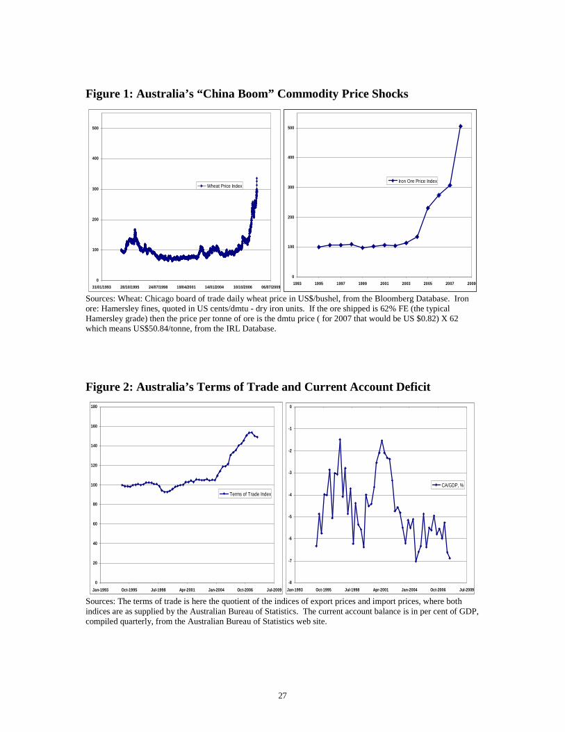
recent “China boom”. The extraordinary nature of the associated commodity price shocks is
clear from Figure 1. Money prices of wheat and iron ore, both major Australian exports, have
risen in the last year or so by several hundreds of per cent. And the shocks go beyond those
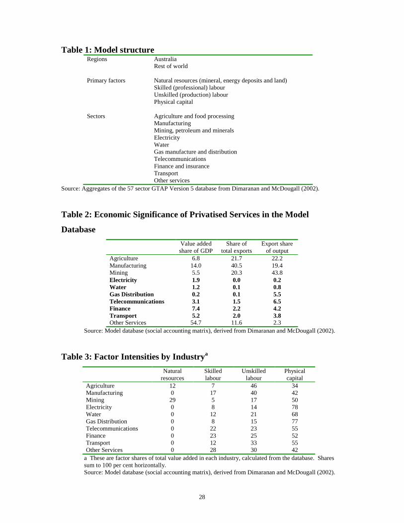
two commodities. Australia’s overall terms of trade rose in this period by 50 per cent, as
shown in Figure 2. At the same time, foreign acquisition of Australian assets has also risen,
almost doubling the current account deficit between the turn of the century and 2007.45 To
examine the effects of these shocks on privatised service performance, we subject the model
to 50 per cent increases in the foreign prices of agricultural products and mining and energy
products, combined with an expansion of the current account deficit by 50 per cent.
45 It must be noted that these extraordinary shocks stem not only from the surge in the growth of China and other “economies in transition”. The US-initiated financial crisis that began in 2007 saw a retreat to commodities, further boosting prices and capital flight from the US.
19
This time we use both a short run closure, in which physical capital is fixed and
specific to each sector and production (unskilled) employment is flexible at a fixed real wage,
and a long run closure in which capital is internationally and intersectorally mobile and
employment is fixed. The number of firms in each sector is held constant in the short run,
allowing pure profits to vary. Two versions of the short run experiment are carried out. In
the first, no price caps are imposed and firms are permitted to choose their mark-ups.46 In the
second, two new initial equilibria are first calculated, by imposing price caps either in all
sectors or in the privatised services only. These price caps are then retained while the
economy is subjected to the China boom shocks in each case. For the long run analysis the
boom shock is first imposed with fixed numbers of firms. Then a new initial equilibrium is
calculated in which entry and exit are allowed and pure profits reduced to zero. To this initial
equilibrium the China boom shocks are applied in such a way as to retain zero pure profits but
to allow entry of new firms.
Taken collectively, in both the short and long runs, these shocks are very positive for
Australia. Their principal short run effects are indicated in the first column of Table 12. Real
GNP, which serves as a preparedness to pay measure given the formulation we use (as
discussed in Section 3), rises significantly, capital returns increase and either real wages or
employment levels rise. There are “Dutch disease” elements, however (Corden and Neary
1982). The natural resource based sectors expand at the expense of manufacturing, which
suffers from higher priced factors and inputs and a real appreciation impairs its competition
against foreign products.47 The service sectors expand, however, sufficiently to raise overall
employment in the short run and real wages in the long run. The only exceptions to this are
electricity and gas, which are large suppliers of inputs to manufacturing. Their gross output
levels and the gross rates of return on their capital fall in both the short and long runs.48
Further insight as to the role of pricing behaviour in this short run simulation is
available from the first column of Table 13. Mark-ups fall in the natural resource based
sectors as the share of elastic exports in the demand they face increases. For the electricity
46 Of course, their strategic interaction is assumed to be constrained by surveillance, which prevents the enlargement of their conjectural variations parameters. 47 These changes are observed in the Australian economy, though the media, with some help from the government, seems to be ignoring the positive in order to build a dismal economic picture. The game of “find the loser” points both to manufacturing firms and employees and to those without housing assets or who are heavily indebted. Any real appreciation requires either inflation or a nominal appreciation. Australia’s central bank prefers the latter, but to bring it about some monetary tightening is required, placing low-margin mortgage holders under pressure. 48 In the short run the fall in these sectors’ rates of return is due to reduced returns on fixed capital. As is shown in Table 13, only in the case of the electricity sector is this effect bolstered by a fall in pure profits, which is due to a strategic decline in the electricity mark-up not matched in the gas sector.
20
sector, the mark-up falls because manufacturing’s relatively inelastic intermediate demand
contracts and so the elasticity it faces rises. With the exception of electricity the privatised
service sectors all experience less elastic demand as the share of intermediate use by natural
resource based sectors (and by each other) expands. This is particularly true of the
telecommunications sector, which raises its mark-up, reduces its output and triples its pure
profits. The boom therefore causes these sectors to exhibit less competitive behaviour that
might be expected to challenge regulatory agencies.
Returning to Table 12, the remaining four columns detail the effects of the China
boom shocks on the economy if price caps are maintained tight enough to eliminate all pure
profits before and after the shocks. The imposition of the caps prevents industries from
raising rents associated with the boom and, as a consequence, the short run gains from the
boom are larger, by amounts that depend on the number of sectors subjected to the price caps.
If all sectors are so regulated, the additional gain is more than a per cent of real GNP. The
real skilled wage would rise by a further two per cent and production employment would rise
by more. Output in the telecommunications sector would then increase, by a substantial three
per cent, but all the services sectors except electricity would expand significantly. If the price
caps were restricted to the privatised services, recalling that these supply about a fifth of
Australia’s GDP, the constraining effects are smaller and the additional boost derived from
the China boom is smaller accordingly. The caps do, nonetheless, yield measurable gains in
economic performance that are evident in the labour markets and in the supply of water, gas,
telecommunications finance and transport services.
Two apparently anomalous results emerge from Table 13. First, the manufacturing
sector, which contracts in both the short and long runs and whose capital suffers declines in
its gross rates of return in both, appears to earn larger pure profits in the short run. Recall
that, in the short run, sectoral capital use is fixed. The overall gross return on manufacturing
capital falls due to its reduced output. But the pure profit share of these returns rises because
manufacturing demand switches away from elastic exports toward inelastic intermediate
markets in the domestic economy. Its overall elasticity of demand falls and its mark-up
therefore rises. The second anomaly is that the boom appears to reduce pure profits in mining
in the short run. In this case the explanation is the reverse of that for the manufacturing
anomaly. A substantial rise in the export share of mining output increases the elasticity of
demand it faces and reduces the mining mark-up. Other things equal, this reduces the pure
profit margin, and this is the dominant short run force.
21
The long run effects of the China boom are quantified in Table 14, with the
implications for competitive behaviour detailed in Table 15. The same general pattern
appears, with substantial overall gains to the economy tempered by the Dutch disease
contraction of manufacturing and associated contractions in the electricity and gas sectors.
The telecommunications sector also contracts, but all the other service sectors expand
strongly. The overall gains are conspicuously smaller when free entry and exit are allowed.
This is because the high profitability the boom brings to most sectors does raise output in the
long run but induces new entry (Table 15) to the point that output per firm actually declines.49
This raises the overall burden of fixed costs. Of course, in the likely event that the boom is
transient, and exit turns out not to be costless, this development would impair the economy’s
future performance.
Returning to the apparently anomalous behaviour of manufacturing profits, in the long
run although the manufacturing mark-up remains high pure profits decline substantially. This
occurs because capital use is flexible at a fixed rate of return in the long run, so lower returns
in manufacturing cause its capital use to decline along with its output. In the first column of
Table 15, however, firm exits are not allowed so that fixed capital use remains constant. On
reduced output, average fixed costs therefore absorb the entire mark-up, causing the decline in
pure profits. In the second column, where entry and exit are free, firm numbers (and therefore
fixed costs) contract by a fifth, helping maintain the zero pure profit equilibrium. In the
mining sector, where pure profits decline in the short run if no price cap is applied (because
the mark-up declines), in the long run variable capital use expands considerably. When entry
is prohibited output also expands and the average fixed cost margin declines. Pure profits
therefore increase considerably (Table 15, first column). When entry is allowed, however,
output and firm numbers expand by similar proportions and so average fixed costs change
little and no new pure profits are earned.
Manufacturing redress?
The negative consequences of the China boom for manufacturing have suggested to
some that its protection should be reinstated, or at least that scheduled declines should be
arrested.50 To address this, we experimented with a rise in the power of the manufacturing
tariff. While differences in the short and long run responses of the whole economy occur due
49 This is clear from a comparison of the changes in gross sectoral output in Table 14 with the corresponding changes in firm numbers in Table 15. 50 Or, at least, that scheduled declines in protection should be halted. See, for example, The Age (2008), VACC (2008).
22
to the complexities of mark-up choice and fixed cost margins discussed above, the dominant
outcome from more manufacturing protection is an economy-wide contraction. Surprisingly,
even the manufacturing sector itself fails to benefit from the tariff increase, both in the short
and long runs. The answer to this further anomaly lies in the manufacturing sector’s pattern
of intermediate use, which is compared with that of other sectors in Table 8.
Of all the sectors manufacturing carries the highest share of intermediate input cost in
total turnover and by far the largest share of manufactured intermediates, a third of which are
imported. So there are two impacts of a tariff rise across the whole manufacturing sector.
First, and strongest, is the effect on intermediate input costs. Second, and weaker, is the
effect of the tariff in raising the price of competing foreign manufactured products. This
effect is weaker because home manufactures are differentiated from foreign ones. Consumer
substitution between them is therefore constrained. The results therefore fail to offer support
for a return to protection to redress inequalities from the China boom. Moreover, because a
tariff rise in so important a tradable goods sector tends to turn the whole economy inward
reducing elasticities of demand, mark-ups rise in all sectors except electricity, transport and
“other services”. And, even though gross rates of return on capital fall across the board in
both the short and long runs, industry scale also falls in all sectors, confirming that such a
policy would doubly impair Australia’s economic efficiency.51
Boom-bust hysteresis
Like all booms, that due to the present surge in Chinese growth is likely to be
transitory. Sooner or later there will be a down-cycle. Yet, because in the up-cycle the
expanding tradable goods sectors bolster demand for services as intermediate inputs and this
demand is less elastic than that for final consumption, the service industries tend to price less
competitively. Boom conditions therefore raise the bar for regulatory institutions. As seen
earlier, the retention of tight price caps, even if only in the privatised services, the benefits to
the economy from the boom are shown be measurably larger enlarges the short run gains from
the boom. Moreover, the boom encourages exits from manufacturing and entries into mining,
agriculture and services, and presumably, the opposite in the following down-cycle. Since
exit costs are non-zero, boom-bust cycles must accompany debilitating hysteresis.52 This
51 Were such a policy to be considered in response to the China boom, for the manufacturing sector to be a clear beneficiary it would need to be given relief from tariffs on its manufactured intermediate inputs. While this would direct the benefits appropriately, the economic cost of the protection would remain large and be borne in other sectors and in labour markets. 52 This is akin to the problem explored by Caballero and Lorenzoni (2007).
23
suggests that, at least for the services sectors, tight price caps serve two key purposes. First,
they enlarge and better distribute the gains during up-cycles and, second, they prevent
excessive entry and hence down-cycle exit costs.
7. Conclusions
An economy-wide model with oligopoly behaviour facilitates the analysis of inter-
sectoral and economy-wide effects of oligopoly rents, suggesting that these are potentially
very large. Taking the extreme of cartelisation in each sector as a benchmark, the complete
exploitation of market power in all sectors is shown to leave the economy smaller by a
quarter. Even if the cartelisation had taken place only in the newly privatised services the
model suggests that Australia’s GDP would have been smaller by a tenth. More particularly,
sectoral interactions due to the exploitation of oligopoly power are shown to be large enough
to justify an economy-wide approach. This is not only true for oligopoly behaviour in the
major sectors of the economy but also in the recently privatised services, supplying as they do
only a fifth of GDP. Moreover, the comparatively small changes in price caps that would
have eliminated 1997’s initial pure profits also cause measurable changes in factor rewards
and the real exchange rate. For the larger sectors tighter price caps have significant effects on
the performance of other sectors, though price caps in the privatised service sectors tend to
cause little interaction between these sectors.
To explore implications for competitive behaviour in the privatised services sectors
and hence their regulation, a final experiment subjects the model to a stylised representation
of the recent China boom. The sheer scale of that boom is made clear, along with its net
positive impacts on the economy as a whole. Because one of its key consequences is an
appreciation of the real exchange rate, however, there is a relative rise in services prices. The
service sectors therefore expand. Yet, because the expanding tradable goods sectors bolster
demand for services as intermediate inputs and this demand is less elastic than that for final
consumption, the service industries tend to price less competitively. Boom conditions are
therefore likely to increase stress on regulatory institutions. If tight price caps could be
retained across the economy, however, even if only in the privatised services, the benefits to
the economy from the boom are shown be measurably larger. Moreover, because strong
“Dutch disease” consequences are unavoidable, the boom encourages exits from
manufacturing and entries into mining, agriculture and services. Since booms are invariably
24
transitory and exit costs are non-zero, boom-bust cycles must accompany debilitating
hysteresis. This suggests some form of assistance to manufacturing during the boom to
prevent excessive exit and tight price caps in services to prevent excessive entry.
References
ABS (2003), Year Book of Australia 2003, Australian Bureau of Statistics, Commonwealth of Australia, Canberra.
Age, The (2008), “Rudd weighs tariff freeze for remaining makers”, http://www.theage.com.au/articles/2008/02/05/1202090421833.html, accessed 4 March 2008.
Australia Daily (2004), “Australia Energy Info”, <http://www.australiadaily.com/s/australiaenergy/> accessed September – October.
ACCC (2003), “ACCC issues consultation notice to Telstra over broadband price-squeeze allegations”, <http://www.accc.gov.au/>.
ACCC (2004), What We Do, Australian Competition and Consumer Commission <http://www.accc.gov.au>.
Balistreri, E.J., R.H. Hillberry and T.J. Rutherford (2007), “Structural estimation and solution of international trademodels with heterogeneous firms”, presented at the 10 Annual Conference on Global Economic Analysis, Purdue University, July.
Bradley, I. and Price, C. (1988) “The economic regulation of private industries by price constraints”, Journal of Industrial Economics, 37:99-106.
Brennan, T. (1989), “Regulating by Capping Prices”, Journal of Regulatory Economics, 1(2): 133-147.
Caballero, R.J. and G. Lorenzoni (2007), “Persistent appreciations and overshooting: a normative analysis”, presented at the 10th Annual International Economics Conference, Santa Cruz Center for International Economics, 5-6 October, University of California at Santa Cruz.
Cabral, L. and M. Riordan (1989), "Incentives for Cost Reduction under Price Cap Regulation," Journal of Regulatory Economics, Springer, 1(2): 93-102, June.
Corden, M. and Neary, P. (1982), “Booming sector and de-industrialization in a small open economy”, The Economic Journal, 92: 825-848.
Courville, L. (1974), “Regulation and efficiency in the electric utility industry”, The Bell Journal of Economics 5(1): 53-74.
Dimaranan, B.V. and McDougall, R.A., 2002. Global Trade, Assistance and Production: the GTAP 5 data base, May, Center for Global Trade Analysis, Purdue University, Lafayette.
Dixon P.B., B.R. Parmenter, J. Sutton and D.P. Vincent (1982), ORANI, a Multi-Sectoral Model of the Australian Economy, Amsterdam: North Holland.
Dixon, P.B. and M. Rimmer (2002), Dynamic General Equilibrium Modelling for Forecasting and Economic Policy, No. 256 in the Contributions for Economic Analysis series, published by Elsevier North Holland.
Doove, S et al (2001), Price Effects of Regulation: International Air Passenger Transport, Telecommunications and Electricity Supply, Productivity Commission Staff Research Paper, AusInfo, Canberra, October.
Findlay, C. (2000), “Introduction to the regulation of services”, in Achieving Better Regulation of Services, Conference Proceedings, Australian National University, 26-27 June.

25
Freed, J. (2004), “Qantas takes huge gamble with Jetstar”, Sydney Morning Herald, May 17. Golley, J.E. (1993), “Pro-competitive effects of trade reform with imperfect competition”,
Honours thesis, School of Economics, Australian National University. Gunasekera, H.D.B. and R. Tyers (1990), "Imperfect Competition and Returns to Scale in a
Newly Industrialising Economy: A General Equilibrium Analysis of Korean Trade Policy", Journal of Development Economics, 34: 223-247.
Harris, R.G. (1984), “Applied general equilibrium analysis of small open economies with scale economies and imperfect competition”, American Economic Review 74: 1016-1032.
Harris, R.G. and D. Cox (1983), Trade, Industrial Policy and Canadian Manufacturing, Toronto: Ontario Economic Council.
Hertel, T.W., (1994), “The ‘pro-competitive effects’ of trade policy reform in a small, open economy”, Journal of International Economics, 36: 391-411.
Horridge, M. (1987), “The long term costs of protection: experimental analysis with different closures of and Australian computable general equilibrium model”, PhD dissertation, University of Melbourne.
Ianchovichina, E., J. Binkley and T.W. Hertel (2000), “Procompetitive effects of foreign competition on domestic markups”, Review of International Economics, 8(1): 134-148.
Littlechild, S.C. (1983), Regulation of British Telecommunications Profitability, Department of Trade and Industry, Government of Great Britain, London.
Melitz, Marc J. (2003), "The Impact of Trade on Intra-Industry Reallocations and Aggregate Industry Productivity," Econometrica, 71(6), 1695-1725.
Menezes, F., R. Breunig, S. Stacey and J. Hornby (2006), “Price regulation in Australia: how consistent has it been?” The Economic Record 82 (256): 67–76.
Moran, A. (2002), “Over-regulation adding fuel to the fire of industry resentment”, The Age, August 26.
NECG (2003) “International Comparison of WACC decisions.” Submission to the Productivity Commission Review of the Gas Access Regime. Available at www.necg.com.au.
OECD (1997), The OECD Report on Regulatory Reform: Summary, Organisation for Economic Cooperation and Development, Paris <http://www.oecd.org/>.
Productivity Commission (1999), Microeconomic Reform and Australian Productivity: Exploring the Links, Productivity Commission Research Paper, AusInfo, Canberra.
_______ and Australian National University (2000), Achieving Better Regulation of Services, Conference Proceedings, AusInfo, Canberra, November.
_______ (2002), Price Regulation of Airport Services, Report no. 19, AusInfo, Canberra. _______ (2003), Regulation and its Review 2002-03, Annual Report Series, Productivity
Commission, Canberra. Rees, L. (2004), “Economy-wide consequences of regulatory reform in an Australian
context”, Honours Thesis, College of Business and Economics, Australian National University.
Short, C., A. Swan, B Graham and W. Mackay-Smith (2001), “Electricity reform: the benefits and costs of Australia”, Outlook 2001: Proceedings of the National Outlook Conference, vol. 3, Minerals and Energy, ABARE, Canberra.
Short, C., A. Heaney and K. Burns (2003), Australian Gas Markets Moving Toward Maturity, Australian Bureau of Agricultural and Resource Economics eReport 03.23, prepared for the Australian Gas Association, Canberra, December.
Sieper, E., (1982), Rationalising Rustic Regulation, Centre for Independent Studies, Sydney.
26
Stigler, G. (1971), “The Theory of Economic Regulation”, The Bell Journal of Economics and Management Science, 2(1): 3-21, Spring.
Telstra (2003), Annual Report. Tyers, R. (2004), “Economy-wide analysis of regulatory and competition policy: a prototype
general equilibrium model”, Working Papers in Economics and Econometrics No. 435, Australian National University, Canberra, January, http://ecocomm.anu.edu.au/ecopapers.
Tyers, R. (2005), “Trade reform and manufacturing pricing behaviour in four archetype Asia-Pacific Economies”, Asian Economic Journal 19(2): 181-203, 2005.
VACC (2008), “Mitsubishi: a message on tariffs”, http://www.vacc.com.au/NewsAdvocacy/MediaReleases/2008/February2008/5FebruaryMitsubishiamessageontariffs/tabid/2514/Default.aspx, accessed 4 March 2008.
Vogelsang, I. and Acton, J. (1989), “Introduction to Symposium on Price-Cap Regulation”, RAND Journal of Economics, 20: 369-72.
Wellisz, S.H. (1963), “Regulation of natural gas pipeline companies: an economic analysis”, Journal of Political Economy 55(1): 30-43.
Xavier, P. (1995), “Price cap regulation for telecommunications: how has it performed in practice?” Telecommunications Policy, 19(8): 599-617.
27
Figure 1: Australia’s “China Boom” Commodity Price Shocks
Sources: Wheat: Chicago board of trade daily wheat price in US$/bushel, from the Bloomberg Database. Iron ore: Hamersley fines, quoted in US cents/dmtu - dry iron units. If the ore shipped is 62% FE (the typical Hamersley grade) then the price per tonne of ore is the dmtu price ( for 2007 that would be US $0.82) X 62 which means US$50.84/tonne, from the IRL Database. Figure 2: Australia’s Terms of Trade and Current Account Deficit
Sources: The terms of trade is here the quotient of the indices of export prices and import prices, where both indices are as supplied by the Australian Bureau of Statistics. The current account balance is in per cent of GDP, compiled quarterly, from the Australian Bureau of Statistics web site.
-8
-7
-6
-5
-4
-3
-2
-1
0
Jan-1993 Oct-1995 Jul-1998 Apr-2001 Jan-2004 Oct-2006 Jul-2009
CA/GDP, %
0
20
40
60
80
100
120
140
160
180
Jan-1993 Oct-1995 Jul-1998 Apr-2001 Jan-2004 Oct-2006 Jul-2009
Terms of Trade Index
0
100
200
300
400
500
1993 1995 1997 1999 2001 2003 2005 2007 2009
Iron Ore Price Index
0
100
200
300
400
500
31/01/1993 28/10/1995 24/07/1998 19/04/2001 14/01/2004 10/10/2006 06/07/2009
Wheat Price Index
28
Table 1: Model structure Regions Australia Rest of world Primary factors Natural resources (mineral, energy deposits and land) Skilled (professional) labour Unskilled (production) labour Physical capital Sectors Agriculture and food processing Manufacturing Mining, petroleum and minerals Electricity Water Gas manufacture and distribution Telecommunications Finance and insurance Transport Other services
Source: Aggregates of the 57 sector GTAP Version 5 database from Dimaranan and McDougall (2002). Table 2: Economic Significance of Privatised Services in the Model
Database
Value added share of GDP
Share of total exports
Export share of output
Agriculture 6.8 21.7 22.2 Manufacturing 14.0 40.5 19.4 Mining 5.5 20.3 43.8 Electricity 1.9 0.0 0.2 Water 1.2 0.1 0.8 Gas Distribution 0.2 0.1 5.5 Telecommunications 3.1 1.5 6.5 Finance 7.4 2.2 4.2 Transport 5.2 2.0 3.8 Other Services 54.7 11.6 2.3
Source: Model database (social accounting matrix), derived from Dimaranan and McDougall (2002). Table 3: Factor Intensities by Industrya
Natural resources
Skilled labour
Unskilled labour
Physical capital
Agriculture 12 7 46 34 Manufacturing 0 17 40 42 Mining 29 5 17 50 Electricity 0 8 14 78 Water 0 12 21 68 Gas Distribution 0 8 15 77 Telecommunications 0 22 23 55 Finance 0 23 25 52 Transport 0 12 33 55 Other Services 0 28 30 42
a These are factor shares of total value added in each industry, calculated from the database. Shares sum to 100 per cent horizontally. Source: Model database (social accounting matrix), derived from Dimaranan and McDougall (2002).
29
Table 4: Conjectural Variations and Initial Elasticity Values Demand elasticities Index of
firm numbersa
Conjectural variations parameter Final Government Intermediate Export
Agriculture 100 0.1 -14.0 -14.0 -7.0 -14.3 Manufacturing 100 0.4 -11.3 -11.3 -5.7 -12.6 Mining 9 0.1 -8.7 -8.7 -6.4 -11.1 Electricity 15 0.6 -7.9 -8.0 -4.0 -9.4 Water 8 0.5 -8.4 -8.4 -4.3 -9.9 Gas Distribution 5 0.7 -6.1 -6.2 -3.1 -8.1 Telecommunications 5 0.8 -5.2 -5.2 -2.7 -7.4 Finance 80 0.5 -9.4 -9.4 -4.7 -10.4 Transport 10 0.6 -6.7 -6.7 -3.4 -8.4 Other Services 100 0.6 -10.5 -10.5 -4.2 -11.3
a This index represents the “effective” number of strategically interacting firms in each sector. Sources: Effective firm numbers and conjectural variations parameters are crude estimates, based on industry concentration, from the Morningstar Financial Analysis Database of listed Australian firms. Elasticities are calculated via the equations in the appendices, where elasticities of substitution sourced from surveys cited by Harris and Cox (1984) and Dimaranan and McDougall (2002).
Table 5: Initial Demand Shares, Average Elasticities and Mark-upsa
Final demand share
Government demand share
Intermediate demand share
Export demand share
Average demand elasticity
Industry mark-upsb
Agriculture 43 0 34 22 -11.7 1.09 Manufacturing 17 0 64 19 -7.9 1.14 Mining 3 1 52 44 -8.6 1.13 Electricity 25 0 75 0 -5.0 1.25 Water 6 3 91 0 -4.7 1.27 Gas Distribution 12 0 83 4 -3.8 1.36 Telecommunications 28 0 65 6 -3.7 1.37 Finance 30 0 66 4 -6.4 1.19 Transport 21 25 50 4 -5.1 1.24 Other Services 45 22 31 2 -8.6 1.13 a All these variables are endogenous in the model. Initial (base) values are provided here. b Industry mark-ups are the ratio of producer prices and average variable costs. Source: Model database (social accounting matrix), derived from Dimaranan and McDougall (2002).
Table 6: Calibrated Pure Profit, Cost Shares and Industry Scale
Per cent of industry turnover Pure profita Fixed costa Variable costa Scaleb Agriculture 0.2 9 91 60 Manufacturing 1.1 12 87 38 Mining 2.1 10 88 41 Electricity 0.8 19 80 21 Water 0.5 20 79 20 Gas distribution 1.6 25 73 15 Telecommunications 1.6 25 73 14 Finance 0.6 15 84 29 Transport 0.9 19 80 22 Other Services 0.1 12 88 41
a The final three columns of the table are calibrated. First, elasticities are estimated, from which mark-up ratios are calculated. The pure profit shares are then used to deduce the fixed cost residual. b Scale is defined as the ratio (in %) of the gross quantity produced and minimum efficient scale, which in turn, is the level of output where unit fixed cost is 5% of unit variable cost. Source: Pure profit proportions are from the Morningstar Financial Analysis Database of listed Australian firms.
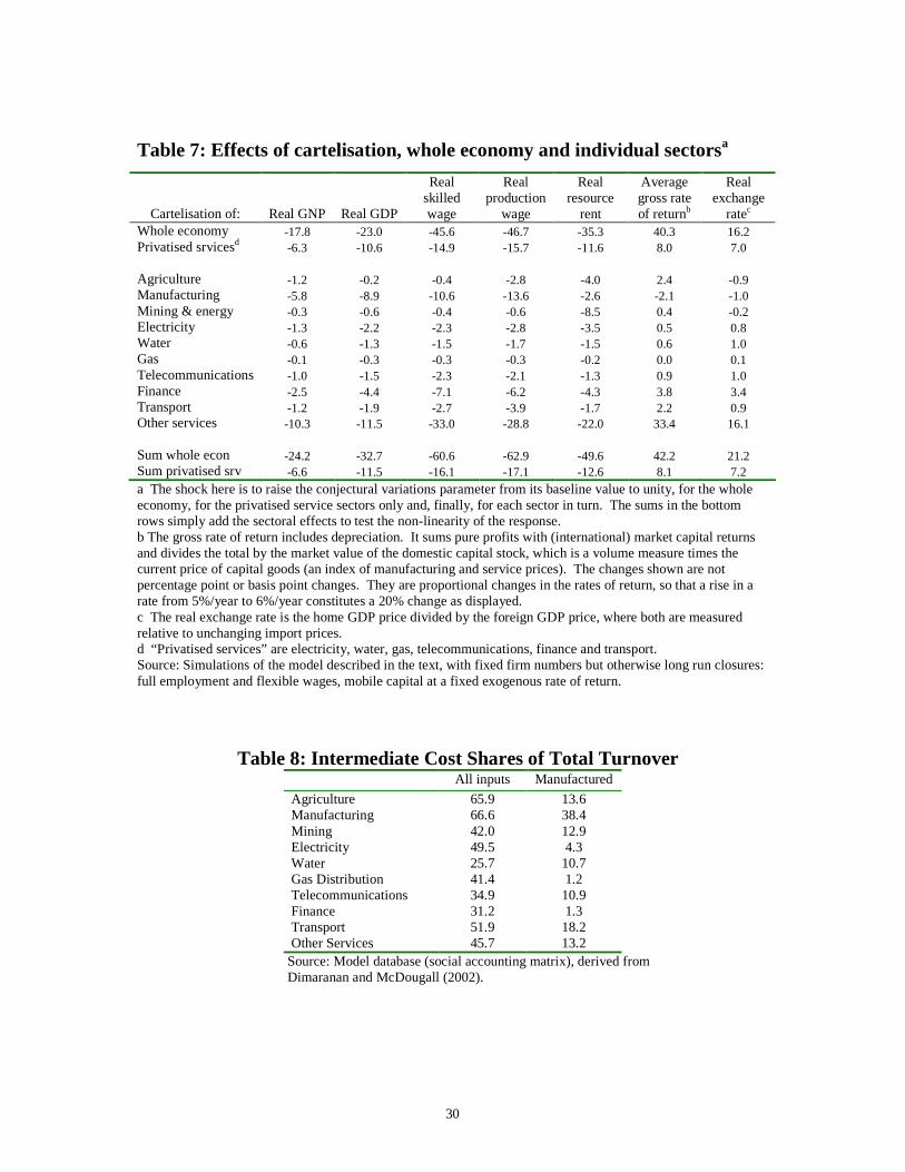
30
Table 7: Effects of cartelisation, whole economy and individual sectorsa
Cartelisation of: Real GNP Real GDP
Real skilled wage
Real production
wage
Real resource
rent
Average gross rate of returnb
Real exchange
ratec
Whole economy -17.8 -23.0 -45.6 -46.7 -35.3 40.3 16.2 Privatised srvicesd -6.3 -10.6 -14.9 -15.7 -11.6 8.0 7.0 Agriculture -1.2 -0.2 -0.4 -2.8 -4.0 2.4 -0.9 Manufacturing -5.8 -8.9 -10.6 -13.6 -2.6 -2.1 -1.0 Mining & energy -0.3 -0.6 -0.4 -0.6 -8.5 0.4 -0.2 Electricity -1.3 -2.2 -2.3 -2.8 -3.5 0.5 0.8 Water -0.6 -1.3 -1.5 -1.7 -1.5 0.6 1.0 Gas -0.1 -0.3 -0.3 -0.3 -0.2 0.0 0.1 Telecommunications -1.0 -1.5 -2.3 -2.1 -1.3 0.9 1.0 Finance -2.5 -4.4 -7.1 -6.2 -4.3 3.8 3.4 Transport -1.2 -1.9 -2.7 -3.9 -1.7 2.2 0.9 Other services -10.3 -11.5 -33.0 -28.8 -22.0 33.4 16.1 Sum whole econ -24.2 -32.7 -60.6 -62.9 -49.6 42.2 21.2 Sum privatised srv -6.6 -11.5 -16.1 -17.1 -12.6 8.1 7.2 a The shock here is to raise the conjectural variations parameter from its baseline value to unity, for the whole economy, for the privatised service sectors only and, finally, for each sector in turn. The sums in the bottom rows simply add the sectoral effects to test the non-linearity of the response. b The gross rate of return includes depreciation. It sums pure profits with (international) market capital returns and divides the total by the market value of the domestic capital stock, which is a volume measure times the current price of capital goods (an index of manufacturing and service prices). The changes shown are not percentage point or basis point changes. They are proportional changes in the rates of return, so that a rise in a rate from 5%/year to 6%/year constitutes a 20% change as displayed. c The real exchange rate is the home GDP price divided by the foreign GDP price, where both are measured relative to unchanging import prices. d “Privatised services” are electricity, water, gas, telecommunications, finance and transport. Source: Simulations of the model described in the text, with fixed firm numbers but otherwise long run closures: full employment and flexible wages, mobile capital at a fixed exogenous rate of return. Table 8: Intermediate Cost Shares of Total Turnover
All inputs Manufactured
Agriculture 65.9 13.6 Manufacturing 66.6 38.4 Mining 42.0 12.9 Electricity 49.5 4.3 Water 25.7 10.7 Gas Distribution 41.4 1.2 Telecommunications 34.9 10.9 Finance 31.2 1.3 Transport 51.9 18.2 Other Services 45.7 13.2
Source: Model database (social accounting matrix), derived from Dimaranan and McDougall (2002).
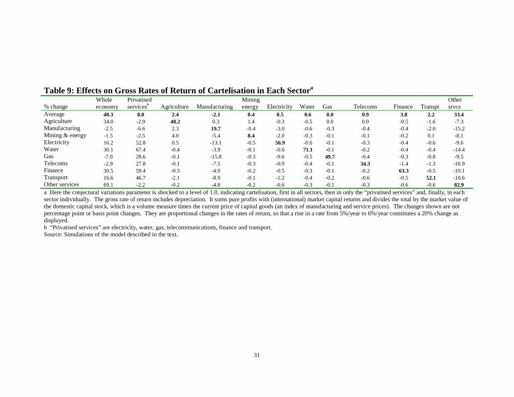
31
Table 9: Effects on Gross Rates of Return of Cartelisation in Each Sectora
% change Whole economy
Privatised servicesb Agriculture Manufacturing
Miningenergy Electricity Water Gas Telecoms Finance Transpt
Other srvcs
Average 40.3 8.0 2.4 -2.1 0.4 0.5 0.6 0.0 0.9 3.8 2.2 33.4 Agriculture 34.0 -2.9 48.2 0.3 1.4 -0.3 -0.5 0.0 0.0 -0.5 -1.6 -7.3 Manufacturing -2.5 -6.6 2.3 19.7 -0.4 -3.0 -0.6 -0.3 -0.4 -0.4 -2.0 -15.2 Mining & energy -1.5 -2.5 4.0 -5.4 8.4 -2.0 -0.3 -0.1 -0.1 -0.2 0.1 -8.1 Electricity 16.2 52.8 0.5 -13.1 -0.5 56.9 -0.6 -0.1 -0.3 -0.4 -0.6 -9.6 Water 30.1 67.4 -0.4 -3.9 -0.1 -0.6 71.1 -0.1 -0.2 -0.4 -0.4 -14.4 Gas -7.0 28.6 -0.1 -15.8 -0.3 -9.6 -0.5 49.7 -0.4 -0.3 -0.8 -9.5 Telecoms -2.9 27.8 -0.1 -7.5 -0.3 -0.9 -0.4 -0.1 34.3 -1.4 -1.3 -16.9 Finance 30.5 59.4 -0.3 -4.0 -0.2 -0.5 -0.3 -0.1 -0.2 63.3 -0.5 -10.1 Transport 16.6 46.7 -2.1 -8.9 -0.1 -1.2 -0.4 -0.2 -0.6 -0.5 52.1 -10.6 Other services 69.1 -2.2 -0.2 -4.8 -0.2 -0.6 -0.3 -0.1 -0.3 -0.6 -0.6 82.9 a Here the conjectural variations parameter is shocked to a level of 1.0, indicating cartelisation, first in all sectors, then in only the “privatised services” and, finally, in each sector individually. The gross rate of return includes depreciation. It sums pure profits with (international) market capital returns and divides the total by the market value of the domestic capital stock, which is a volume measure times the current price of capital goods (an index of manufacturing and service prices). The changes shown are not percentage point or basis point changes. They are proportional changes in the rates of return, so that a rise in a rate from 5%/year to 6%/year constitutes a 20% change as displayed. b “Privatised services” are electricity, water, gas, telecommunications, finance and transport. Source: Simulations of the model described in the text.
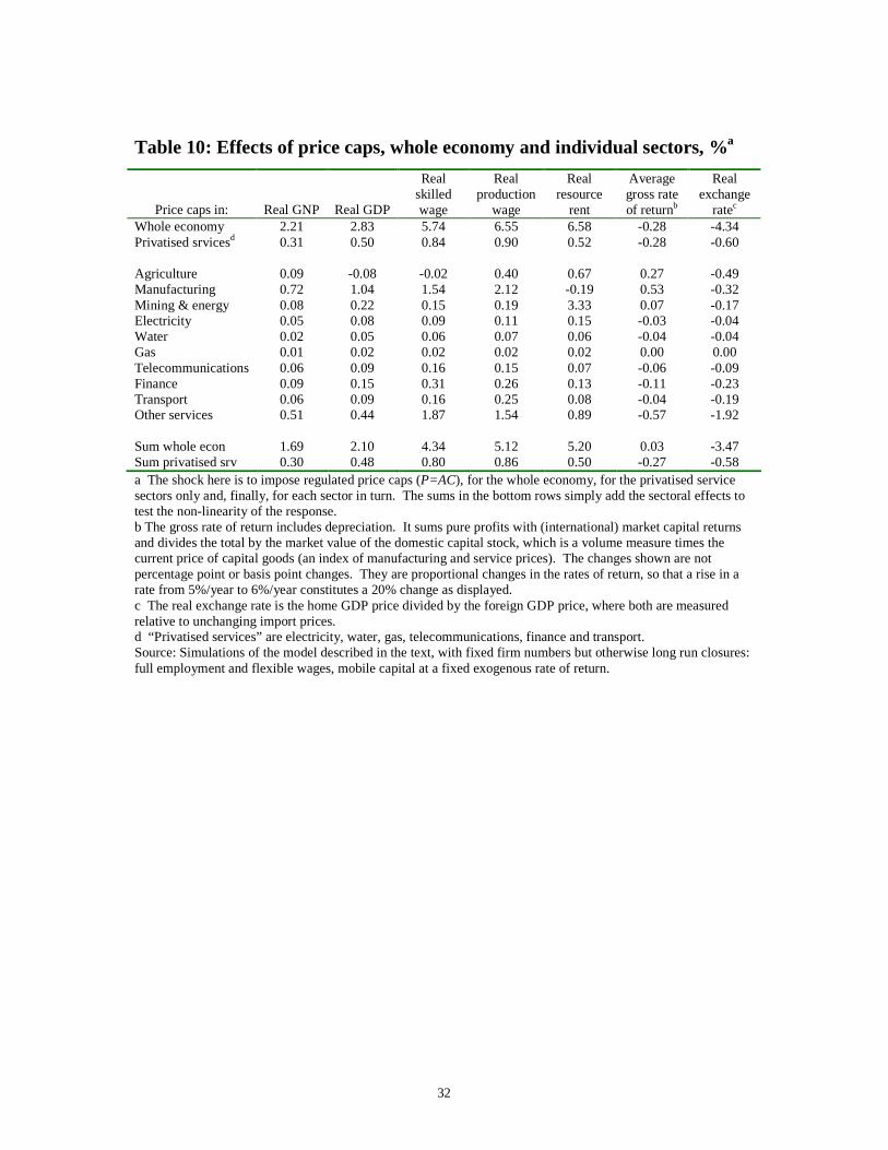
32
Table 10: Effects of price caps, whole economy and individual sectors, %a
Price caps in: Real GNP Real GDP
Real skilled wage
Real production
wage
Real resource
rent
Average gross rate of returnb
Real exchange
ratec
Whole economy 2.21 2.83 5.74 6.55 6.58 -0.28 -4.34 Privatised srvicesd 0.31 0.50 0.84 0.90 0.52 -0.28 -0.60 Agriculture 0.09 -0.08 -0.02 0.40 0.67 0.27 -0.49 Manufacturing 0.72 1.04 1.54 2.12 -0.19 0.53 -0.32 Mining & energy 0.08 0.22 0.15 0.19 3.33 0.07 -0.17 Electricity 0.05 0.08 0.09 0.11 0.15 -0.03 -0.04 Water 0.02 0.05 0.06 0.07 0.06 -0.04 -0.04 Gas 0.01 0.02 0.02 0.02 0.02 0.00 0.00 Telecommunications 0.06 0.09 0.16 0.15 0.07 -0.06 -0.09 Finance 0.09 0.15 0.31 0.26 0.13 -0.11 -0.23 Transport 0.06 0.09 0.16 0.25 0.08 -0.04 -0.19 Other services 0.51 0.44 1.87 1.54 0.89 -0.57 -1.92 Sum whole econ 1.69 2.10 4.34 5.12 5.20 0.03 -3.47 Sum privatised srv 0.30 0.48 0.80 0.86 0.50 -0.27 -0.58 a The shock here is to impose regulated price caps (P=AC), for the whole economy, for the privatised service sectors only and, finally, for each sector in turn. The sums in the bottom rows simply add the sectoral effects to test the non-linearity of the response. b The gross rate of return includes depreciation. It sums pure profits with (international) market capital returns and divides the total by the market value of the domestic capital stock, which is a volume measure times the current price of capital goods (an index of manufacturing and service prices). The changes shown are not percentage point or basis point changes. They are proportional changes in the rates of return, so that a rise in a rate from 5%/year to 6%/year constitutes a 20% change as displayed. c The real exchange rate is the home GDP price divided by the foreign GDP price, where both are measured relative to unchanging import prices. d “Privatised services” are electricity, water, gas, telecommunications, finance and transport. Source: Simulations of the model described in the text, with fixed firm numbers but otherwise long run closures: full employment and flexible wages, mobile capital at a fixed exogenous rate of return.
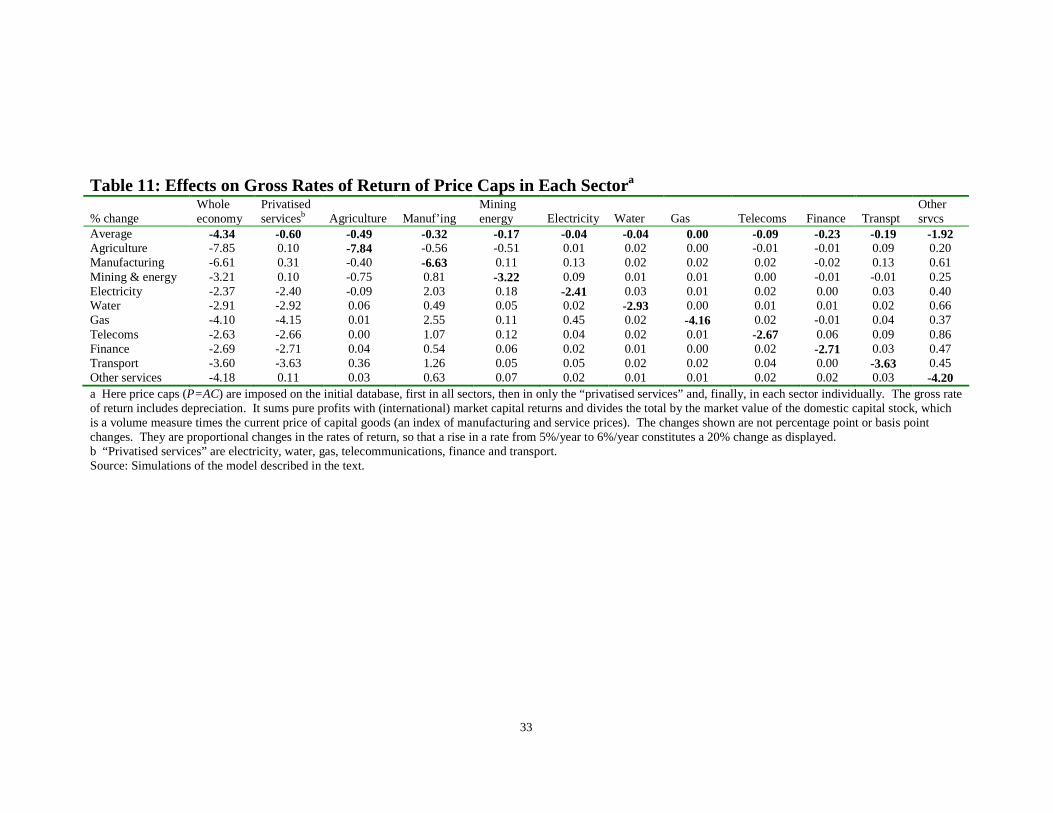
33
Table 11: Effects on Gross Rates of Return of Price Caps in Each Sectora
% change Whole economy
Privatised servicesb Agriculture Manuf’ing
Mining energy Electricity Water Gas Telecoms Finance Transpt
Other srvcs
Average -4.34 -0.60 -0.49 -0.32 -0.17 -0.04 -0.04 0.00 -0.09 -0.23 -0.19 -1.92 Agriculture -7.85 0.10 -7.84 -0.56 -0.51 0.01 0.02 0.00 -0.01 -0.01 0.09 0.20 Manufacturing -6.61 0.31 -0.40 -6.63 0.11 0.13 0.02 0.02 0.02 -0.02 0.13 0.61 Mining & energy -3.21 0.10 -0.75 0.81 -3.22 0.09 0.01 0.01 0.00 -0.01 -0.01 0.25 Electricity -2.37 -2.40 -0.09 2.03 0.18 -2.41 0.03 0.01 0.02 0.00 0.03 0.40 Water -2.91 -2.92 0.06 0.49 0.05 0.02 -2.93 0.00 0.01 0.01 0.02 0.66 Gas -4.10 -4.15 0.01 2.55 0.11 0.45 0.02 -4.16 0.02 -0.01 0.04 0.37 Telecoms -2.63 -2.66 0.00 1.07 0.12 0.04 0.02 0.01 -2.67 0.06 0.09 0.86 Finance -2.69 -2.71 0.04 0.54 0.06 0.02 0.01 0.00 0.02 -2.71 0.03 0.47 Transport -3.60 -3.63 0.36 1.26 0.05 0.05 0.02 0.02 0.04 0.00 -3.63 0.45 Other services -4.18 0.11 0.03 0.63 0.07 0.02 0.01 0.01 0.02 0.02 0.03 -4.20 a Here price caps (P=AC) are imposed on the initial database, first in all sectors, then in only the “privatised services” and, finally, in each sector individually. The gross rate of return includes depreciation. It sums pure profits with (international) market capital returns and divides the total by the market value of the domestic capital stock, which is a volume measure times the current price of capital goods (an index of manufacturing and service prices). The changes shown are not percentage point or basis point changes. They are proportional changes in the rates of return, so that a rise in a rate from 5%/year to 6%/year constitutes a 20% change as displayed. b “Privatised services” are electricity, water, gas, telecommunications, finance and transport. Source: Simulations of the model described in the text.
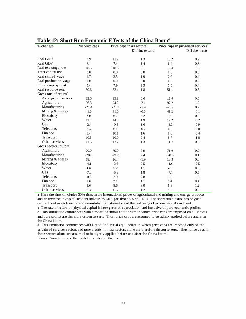
34
Table 12: Short Run Economic Effects of the China Booma
% changes No price caps Price caps in all sectorsc Price caps in privatised servicesd Diff due to caps Diff due to caps Real GNP 9.9 11.2 1.3 10.2 0.2 Real GDP 6.1 7.4 1.4 6.4 0.3 Real exchange rate 18.5 18.6 0.1 18.4 -0.1 Total capital use 0.0 0.0 0.0 0.0 0.0 Real skilled wage 1.7 3.5 1.9 2.0 0.4 Real production wage 0.0 0.0 0.0 0.0 0.0 Prodn employment 5.4 7.9 2.5 5.8 0.4 Real resource rent 50.6 52.4 1.8 51.1 0.5 Gross rate of returnb Average, all sectors 12.6 13.1 0.6 12.6 0.0 Agriculture 96.3 94.2 -2.1 97.2 1.0 Manufacturing -21.4 -23.3 -1.9 -21.2 0.2 Mining & energy 41.3 41.0 -0.3 41.2 -0.1 Electricity 3.0 6.2 3.2 3.9 0.9 Water 12.4 14.3 1.9 12.2 -0.2 Gas -2.4 -0.8 1.6 -3.3 -0.9 Telecoms 6.3 6.1 -0.2 4.2 -2.0 Finance 8.4 10.1 1.6 8.0 -0.4 Transport 10.5 10.9 0.4 8.7 -1.8 Other services 11.5 12.7 1.3 11.7 0.2 Gross sectoral output Agriculture 70.0 79.0 8.9 71.0 0.9 Manufacturing -28.6 -26.3 2.4 -28.6 0.1 Mining & energy 18.4 16.4 -1.9 18.3 0.0 Electricity -4.1 -3.6 0.5 -4.6 -0.5 Water 4.6 5.7 1.1 4.9 0.3 Gas -7.6 -5.8 1.8 -7.1 0.5 Telecoms -0.8 2.0 2.8 1.0 1.8 Finance 1.0 2.1 1.1 1.4 0.4 Transport 5.6 8.6 3.0 6.8 1.2 Other services 5.3 6.5 1.2 5.5 0.2 a Here the shock includes 50% rises in the international prices of agricultural and mining and energy products and an increase in capital account inflows by 50% (or about 5% of GDP). The short run closure has physical capital fixed in each sector and immobile internationally and the real wage of production labour fixed. b The rate of return on physical capital is here gross of depreciation and inclusive of pure economic profits. c This simulation commences with a modified initial equilibrium in which price caps are imposed on all sectors and pure profits are therefore driven to zero. Thus, price caps are assumed to be tightly applied before and after the China boom. d This simulation commences with a modified initial equilibrium in which price caps are imposed only on the privatised services sectors and pure profits in those sectors alone are therefore driven to zero. Thus, price caps in these sectors alone are assumed to be tightly applied before and after the China boom. Source: Simulations of the model described in the text.
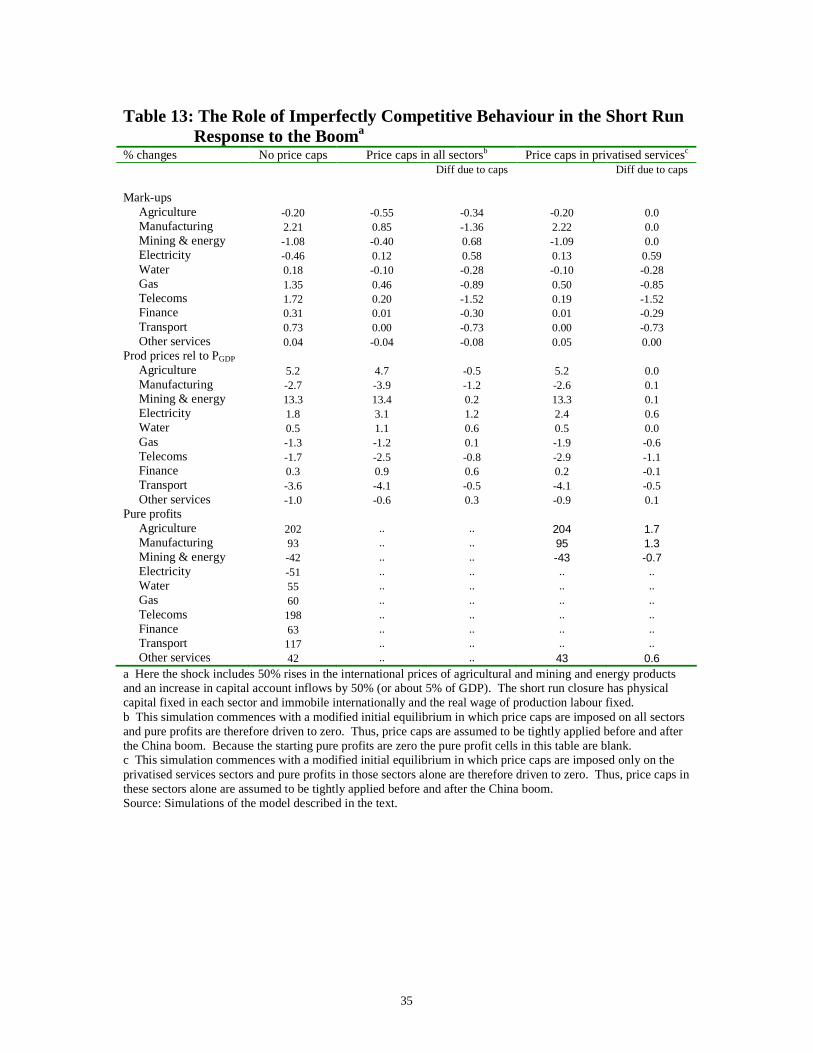
35
Table 13: The Role of Imperfectly Competitive Behaviour in the Short Run
Response to the Booma
% changes No price caps Price caps in all sectorsb Price caps in privatised servicesc Diff due to caps Diff due to caps Mark-ups Agriculture -0.20 -0.55 -0.34 -0.20 0.0 Manufacturing 2.21 0.85 -1.36 2.22 0.0 Mining & energy -1.08 -0.40 0.68 -1.09 0.0 Electricity -0.46 0.12 0.58 0.13 0.59 Water 0.18 -0.10 -0.28 -0.10 -0.28 Gas 1.35 0.46 -0.89 0.50 -0.85 Telecoms 1.72 0.20 -1.52 0.19 -1.52 Finance 0.31 0.01 -0.30 0.01 -0.29 Transport 0.73 0.00 -0.73 0.00 -0.73 Other services 0.04 -0.04 -0.08 0.05 0.00 Prod prices rel to PGDP Agriculture 5.2 4.7 -0.5 5.2 0.0 Manufacturing -2.7 -3.9 -1.2 -2.6 0.1 Mining & energy 13.3 13.4 0.2 13.3 0.1 Electricity 1.8 3.1 1.2 2.4 0.6 Water 0.5 1.1 0.6 0.5 0.0 Gas -1.3 -1.2 0.1 -1.9 -0.6 Telecoms -1.7 -2.5 -0.8 -2.9 -1.1 Finance 0.3 0.9 0.6 0.2 -0.1 Transport -3.6 -4.1 -0.5 -4.1 -0.5 Other services -1.0 -0.6 0.3 -0.9 0.1 Pure profits Agriculture 202 .. .. 204 1.7 Manufacturing 93 .. .. 95 1.3 Mining & energy -42 .. .. -43 -0.7 Electricity -51 .. .. .. .. Water 55 .. .. .. .. Gas 60 .. .. .. .. Telecoms 198 .. .. .. .. Finance 63 .. .. .. .. Transport 117 .. .. .. .. Other services 42 .. .. 43 0.6 a Here the shock includes 50% rises in the international prices of agricultural and mining and energy products and an increase in capital account inflows by 50% (or about 5% of GDP). The short run closure has physical capital fixed in each sector and immobile internationally and the real wage of production labour fixed. b This simulation commences with a modified initial equilibrium in which price caps are imposed on all sectors and pure profits are therefore driven to zero. Thus, price caps are assumed to be tightly applied before and after the China boom. Because the starting pure profits are zero the pure profit cells in this table are blank. c This simulation commences with a modified initial equilibrium in which price caps are imposed only on the privatised services sectors and pure profits in those sectors alone are therefore driven to zero. Thus, price caps in these sectors alone are assumed to be tightly applied before and after the China boom. Source: Simulations of the model described in the text.
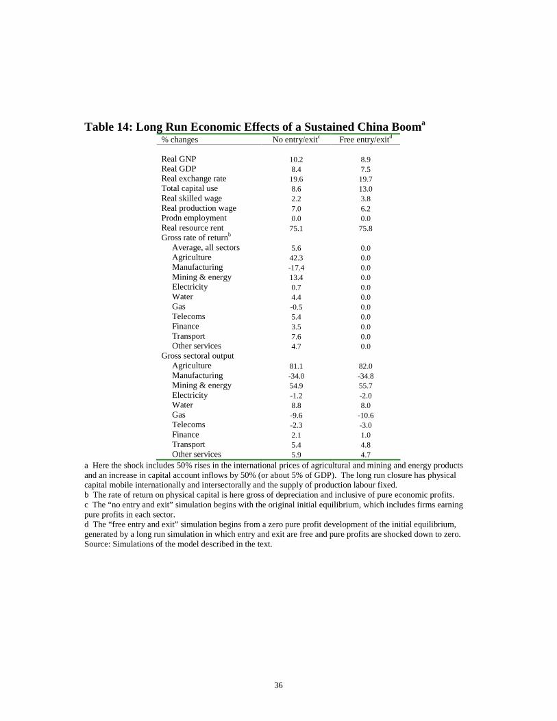
36
Table 14: Long Run Economic Effects of a Sustained China Booma
% changes No entry/exitc Free entry/exitd Real GNP 10.2 8.9 Real GDP 8.4 7.5 Real exchange rate 19.6 19.7 Total capital use 8.6 13.0 Real skilled wage 2.2 3.8 Real production wage 7.0 6.2 Prodn employment 0.0 0.0 Real resource rent 75.1 75.8 Gross rate of returnb Average, all sectors 5.6 0.0 Agriculture 42.3 0.0 Manufacturing -17.4 0.0 Mining & energy 13.4 0.0 Electricity 0.7 0.0 Water 4.4 0.0 Gas -0.5 0.0 Telecoms 5.4 0.0 Finance 3.5 0.0 Transport 7.6 0.0 Other services 4.7 0.0 Gross sectoral output Agriculture 81.1 82.0 Manufacturing -34.0 -34.8 Mining & energy 54.9 55.7 Electricity -1.2 -2.0 Water 8.8 8.0 Gas -9.6 -10.6 Telecoms -2.3 -3.0 Finance 2.1 1.0 Transport 5.4 4.8 Other services 5.9 4.7
a Here the shock includes 50% rises in the international prices of agricultural and mining and energy products and an increase in capital account inflows by 50% (or about 5% of GDP). The long run closure has physical capital mobile internationally and intersectorally and the supply of production labour fixed. b The rate of return on physical capital is here gross of depreciation and inclusive of pure economic profits. c The “no entry and exit” simulation begins with the original initial equilibrium, which includes firms earning pure profits in each sector. d The “free entry and exit” simulation begins from a zero pure profit development of the initial equilibrium, generated by a long run simulation in which entry and exit are free and pure profits are shocked down to zero. Source: Simulations of the model described in the text.
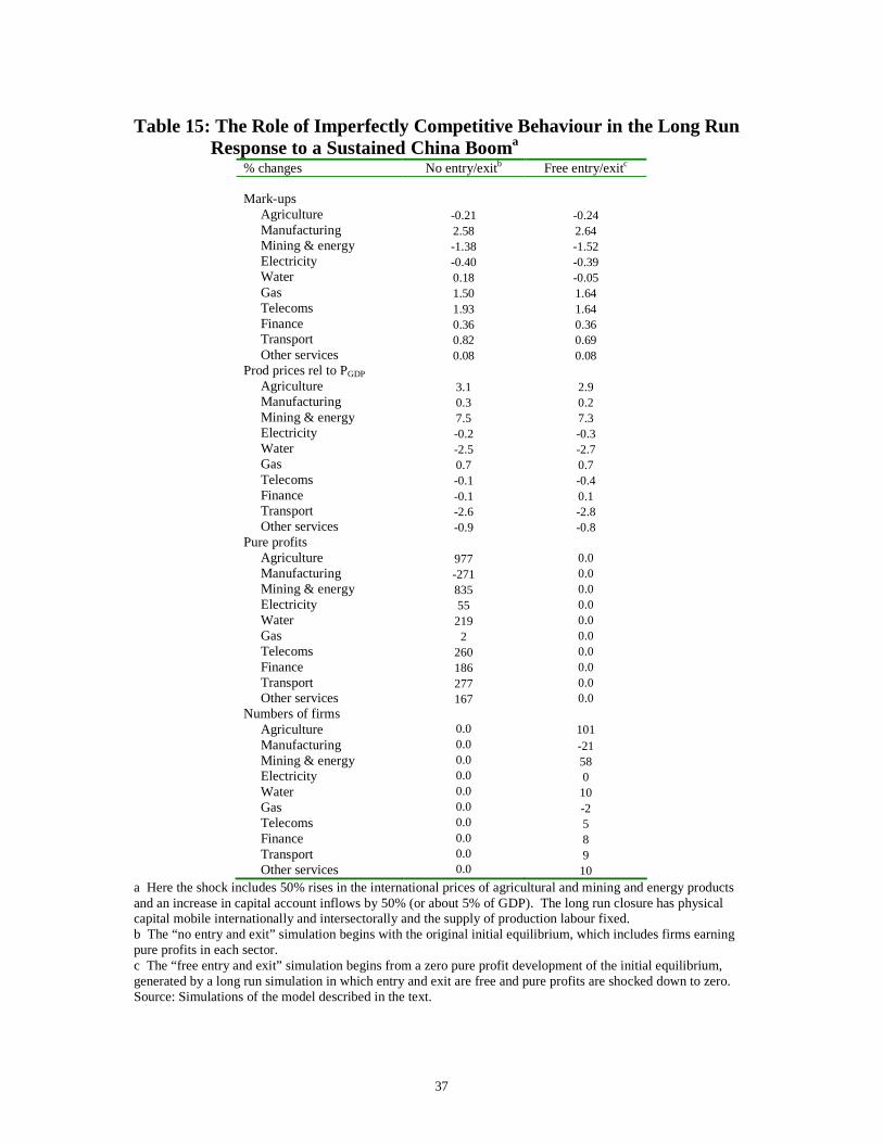
37
Table 15: The Role of Imperfectly Competitive Behaviour in the Long Run
Response to a Sustained China Booma
% changes No entry/exitb Free entry/exitc Mark-ups Agriculture -0.21 -0.24 Manufacturing 2.58 2.64 Mining & energy -1.38 -1.52 Electricity -0.40 -0.39 Water 0.18 -0.05 Gas 1.50 1.64 Telecoms 1.93 1.64 Finance 0.36 0.36 Transport 0.82 0.69 Other services 0.08 0.08 Prod prices rel to PGDP Agriculture 3.1 2.9 Manufacturing 0.3 0.2 Mining & energy 7.5 7.3 Electricity -0.2 -0.3 Water -2.5 -2.7 Gas 0.7 0.7 Telecoms -0.1 -0.4 Finance -0.1 0.1 Transport -2.6 -2.8 Other services -0.9 -0.8 Pure profits Agriculture 977 0.0 Manufacturing -271 0.0 Mining & energy 835 0.0 Electricity 55 0.0 Water 219 0.0 Gas 2 0.0 Telecoms 260 0.0 Finance 186 0.0 Transport 277 0.0 Other services 167 0.0 Numbers of firms Agriculture 0.0 101 Manufacturing 0.0 -21 Mining & energy 0.0 58 Electricity 0.0 0 Water 0.0 10 Gas 0.0 -2 Telecoms 0.0 5 Finance 0.0 8 Transport 0.0 9 Other services 0.0 10
a Here the shock includes 50% rises in the international prices of agricultural and mining and energy products and an increase in capital account inflows by 50% (or about 5% of GDP). The long run closure has physical capital mobile internationally and intersectorally and the supply of production labour fixed. b The “no entry and exit” simulation begins with the original initial equilibrium, which includes firms earning pure profits in each sector. c The “free entry and exit” simulation begins from a zero pure profit development of the initial equilibrium, generated by a long run simulation in which entry and exit are free and pure profits are shocked down to zero. Source: Simulations of the model described in the text.
38
Appendix 1: The Model in Detail
We model the real economy and so incorporate no markets for money or other assets.
An exchange rate is defined primarily as a solution device. Its value adjusts to satisfy a
balance of payments condition, thereby bringing about changes in relative domestic prices.
Most often, however, the balance of payments condition is eliminated from the model by a
closure adjustment, and the artificial exchange rate fixed, so that all the adjustments to shocks
are made by the home prices relative to the bundle of imported products as the numeraire.
The balance of payments condition is still met because it is implied by the household’s and
the government’s budget constraints. The artificial exchange rate serves no valuable purpose
as a product of model since what matters for trade and relative service sector performance is
the real exchange rate – the “common currency” (in this case “common numeraire”) average
price of home relative to foreign products and services.
Demand elasticities
These depend on the structure of the model, to be detailed below. They are essential
to the capture of oligopoly behaviour since they determine the size of mark-up ratios, via
equations (1) and (5) in the main text. For final demand the elasticity expression is:
(A1.1) ( )�
�( ) ( )( )
(1 )
11 1 1
Fi
iHF F F F F Fi i i i i i i iF
i i
Pn
n P
σ
ε η σ δ η σ µ− = − + − + − + −
,
where Fiη is the elasticity of substitution of final demand across home varieties in sector i, F
iδ
is the home share in final demand for product i, Fiσ is the elasticity of substitution of final
demand for good i between domestic and foreign countries, in is the number of domestic
firms in industry i, iHP is the CES composite price of all home varieties of product i, and ˆ FiP
is the CES composite of home and foreign final product prices in the domestic market,
weighted by domestic consumption shares. Equation (A1.1) is derived in Appendix 2.
For exports it is assumed that home firms face such competition in foreign markets
that non-collusive pricing behaviour in necessitated. The foreign demand elasticity takes the
same form as (A1.1), except that the foreign conjectural variation parameter,Xiµ , is zero:
39
(A1.2) ( )�
( ) ( )( )(1 )
11 1 1
ˆ
Xie
iX X X X X Xi i i i i i i iX
i i
Pn
n P
σ
ε η σ θ η σ µ− = − + − + − + −
( )�
( )(1 )
11
ˆ
Xie
iX X X Xi i i i iX
i i
P
n P
σ
η σ θ η σ− = − + − + −
,
where ˆ eiP is the CES composite foreign currency price of all exported varieties of product I
and ˆ XiP is the CES composite of exported and competing foreign final product prices in the
foreign market, weighted by foreign consumption shares. Foreigners differentiate home
exports from corresponding foreign products with elasticity of substitution Xiσ and home
varieties from one another with elasticity of substitution Xiη .
For the intermediate demand elasticity a similar expression is obtained:
(A1.3) �
( ) ( )( )1
1
1( 1) 1 1
ˆ
Ii
NiHI I I I I I
i ij i ij i ij i i i iIj i i
Ps n
n P
σ
ε η γ σ φ η σ µ−
=
= − + + − + − + −
∑ ,
where sijI is the share of industry j in the total intermediate demand for input i and ˆ I
iP is the
CES composite of home and foreign intermediate product prices in the domestic market,
weighted by domestic intermediate consumption shares.. The corresponding expression for
the elasticity of government demand is:
(A1.4) ( )�
( ) ( )( )(1 )
11 1 1
ˆ
Gi
iHG G G G G Gi i i i i i i iG
i i
Pn
n P
σ
ε η σ δ η σ µ− = − + − + − + −
.
Mark-ups:
We assume constant marginal cost oligopolistic firms in differentiated product
markets. Symmetry within each sector implies a common optimal unregulated mark-up for
each firm, as in equation (1) of the main text.
Domestic prices of imported goods:
These are:
(A1.5) * (1 )(1 )w M Ci i i
i
pp
e
τ τ+ +=
40
where wip is the exogenous foreign currency price of goods produced in the rest of the world,
Miτ is the ad valorem tariff rate and C
iτ is the indirect consumption tax in industry i.
Domestic prices of home products:
As in equation (1) of the main text, these are marked up over average variable cost.
To obtain average variable cost, recall that production is Cobb-Douglas in variable factors and
inputs, with output elasticities αi for capital, βki for factors k and γji for inputs j and that the
subaggregation of imported and domestic inputs is CES. Unit variable costs are therefore
calculated as:
(A1.6) 1 1
ˆ jii ki
K NI
i i k jik j
v b r w P iγα β
= =
= ∀ ∏ ∏ .
where the scale coefficient bi is calibrated from the SAM, as are all the exponents in the
equation, and IjiP is a CES composite of home and imported input prices weighted by the
domestic and imported shares specific to consuming industry i:
(A1.7) ( ) ( )1
(1 )(1 ) 1*ˆ (1 )II Ijj jI
ji ji j ji jP p pσσ σφ φ
−− − = + − ,
where jiφ is the domestic share of inputs from industry j in use by industry i. Then, domestic
producer prices are simply higher by the mark-up, mi: ,i i ip m v i= ∀ .
Unit factor and input demands:
These are derived by solving the firm’s cost minimisation problem with Cobb-
Douglas production in variable factors and inputs. It is assumed that firms have no
monopsony power in either factor or input markets. Therefore, the unit factor demands for
capital and other factors are:
(A1.8) ,K i ii
vu i
r
α= ∀ and ,L ki iki
k
vu k i
w
β= ∀ ,
where k denotes non-capital factors which are natural resources and skilled and unskilled
labour.
The corresponding unit input demands are Leontief input-output coefficients, except
that their values depend on product and input prices. For home-produced and imported inputs
from industry i used in the product of industry j, respectively they are:
41
(A1.9) *
* (1 ), ,
ˆ ˆ ˆ ˆ
I Ii i
ij j ij ji iij ij ij ijI I I I
ij ij ij ij
v vp pA A i j
P P P P
σ σφ φ
γ γ− −
−= = ∀
.
Prices of home product exports in foreign markets:
These are in foreign currency so they depend on the home producer price, the
exchange rate, the export subsidy rate Xis and the foreign import tariff rate, * M
iτ :
(A1.10) *(1 )
(1 )i
Me i i
i X
p ep i
s
τ+= ∀+
.
Export demand:
Foreigners differentiate home exports from corresponding foreign products with
elasticity of substitution Xiσ (>0) and home varieties from one another with elasticity of
substitution Xiη . This gives the following expression for foreign demand for variety j of
home product i:
(A1.11) �
�ˆ ˆ
X Xi ie
i iHji iij eX X
i i i i
pE PX
n P P P
σ ηθ
− − =
,
where iθ is the calibrated reference share of the home export in total consumption, Ei is a
calibrated constant representing foreign expenditure on exports from industry i, and ˆ XiP is a
CES composite of the home export price, eip , and the foreign product price, wip , in the
foreign market, weighted by foreign consumption shares.
Final demand:
Home consumers differentiate home products from corresponding foreign products
with elasticity of substitution Fiσ (>0) and home varieties from one another with elasticity of
substitution Fiη . They have Cobb-Douglas utility in broad product groups, with the result that
expenditure shares are constant across these groups. Final demand for variety j of home
product group i is therefore:
(A1.12) �
�ˆ ˆ
F Fi iF F
iH iHji i YiHj F F
iHi i i
pa Y T PD
n P P P
σ ηδ
− − −=
.
42
where aiF is the calibrated reference expenditure share of product group i, F
iδ is the
corresponding share of home goods in final demand for product i, Y is GNP, TY is total direct
(income) tax, and the composite price is:
(A1.13) ( ) (1 )
1
1(1 ) *ˆ ( ) 1 ( )F FF i iiF F F
i i iH i iP p pσ σσδ δ
− −− = + −
,
where the home share is Fiδ . The expression for imports is correspondingly given by:
(A1.14) *
(1 )ˆ ˆ
Fi
F F F iYi i i F F
i i
pY TM a
P P
σ
δ−
−= −
Government demand:
The formulation adopted is similar to that for final demand by households.
Government demand for home produced products and imports, respectively, is given by:
(A1.15) �
�ˆ ˆ
G Gi iG G
iH iHji iiHj G G
iHi i i
pa G PG
n P P P
σ ηδ
− −
= ,
( )*
* 1ˆ ˆ
Gi
G G ii i i G G
i i
pGG a
P P
σ
δ−
= −
,
where the composite price of government purchases is:
(A1.16) ( ) ( )(1 )
1
1(1 ) *ˆ (1 )G GiG iiG G G
i i i i iP p pσ σσδ δ
− −− = + −
It is assumed that the government spends all it receives in tax revenues. That is, it maintains a
balanced budget. The model is comparative static and it does not at present incorporate
private or public savings and investment.53
Demand for inputs:
This is derived from the input-output coefficients and gross industry output, Q.
Demands for home-produced and imported varieties of the intermediate good i are:
(A1.17) * *
1 1
,N N
i ij j i ij jj j
I A Q I A Q i= =
= = ∀∑ ∑
53 The implicit assumption being that the sectoral composition of investment spending is the same as that of final demand.

43
Tax revenue:
The government raises tax revenue from both direct and indirect taxation. The
revenue raised from each source is expressed below.
Direct income tax revenue
(A1.18) ( )1
i
N
Y K i i U U U S S Si
T rK w L w Lτ π τ τ=
= + + +∑ ,
where Ki denotes total capital stock in industry i, iπ denotes total pure profit in industry i,
“U” denotes unskilled labour and “S” denotes skilled labour. Note that the tax rate on capital
income is not generic. This enables the capture of tax policies that discriminate between
sectors.
Consumption tax revenue
(A1.19) *
1 1
N NC C
C i i i i i ii i
T p D p Mτ τ= =
= +∑ ∑
Import tariff revenue
(A1.20) *
1
( )wN
M iM i i i
i
pT M I
eτ
=
= +∑
Export tax revenue
(A1.21) 1
( )N
XX i i i
i
T s p X=
= −∑ ,
where Xis denotes the net power of the export subsidy rate.
Total tax revenue is then simply a sum of the individual components above.
Economic profits or losses:
This is revenue derived from mark-ups over unit variable costs, less total fixed costs.
For sector i it is:
(A1.22) ( ) ( )K Li i i i i i S ip v Q n r f w f iπ = − − + ∀ ,
where ni is the number of firms, fiK is the fixed capital requirement per firm and fi
L is the fixed
skilled labour requirement per firm in sector i. Net profit in industry i is therefore:
(A1.23) ( )( ) ( ) 1N K L Ki i i i i i S i ip v Q n r f w f iπ τ = − − + − ∀
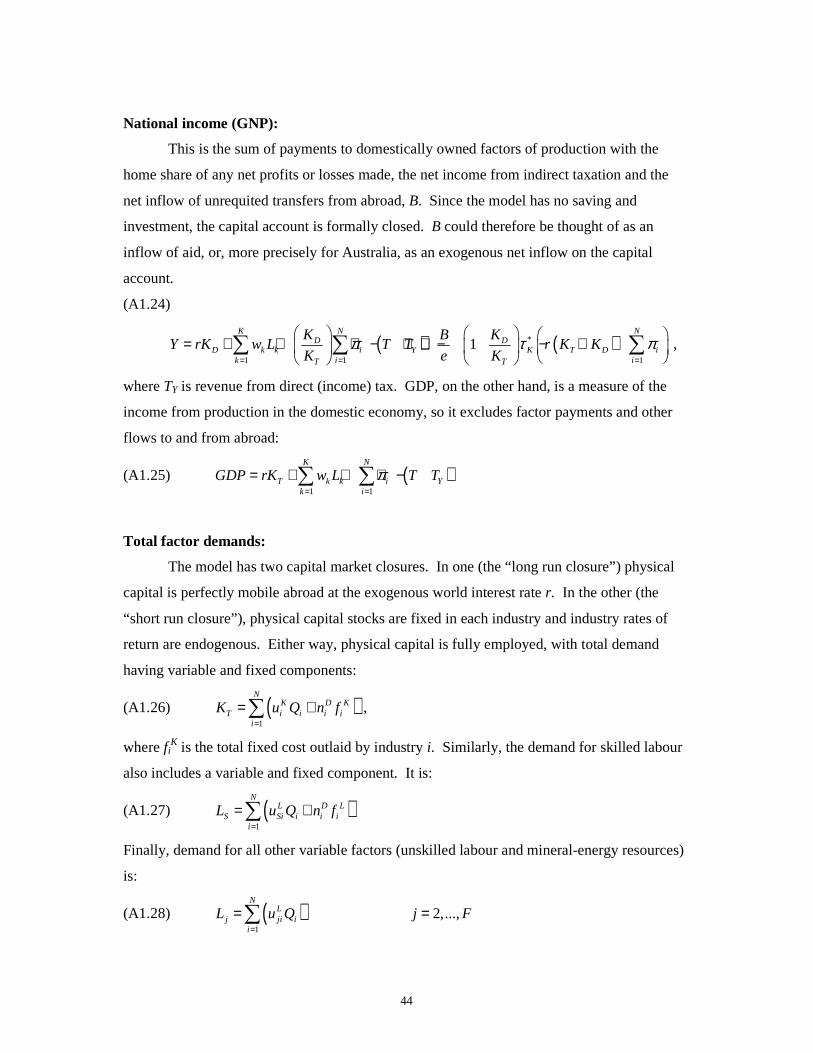
44
National income (GNP):
This is the sum of payments to domestically owned factors of production with the
home share of any net profits or losses made, the net income from indirect taxation and the
net inflow of unrequited transfers from abroad, B. Since the model has no saving and
investment, the capital account is formally closed. B could therefore be thought of as an
inflow of aid, or, more precisely for Australia, as an exogenous net inflow on the capital
account.
(A1.24)
( ) ( )*
1 1 1
1K N N
D DD k k i Y K T D i
k i iT T
K KBY rK w L T T r K K
K e Kπ τ π
= = =
= + + + − + + − − +
∑ ∑ ∑ ,
where TY is revenue from direct (income) tax. GDP, on the other hand, is a measure of the
income from production in the domestic economy, so it excludes factor payments and other
flows to and from abroad:
(A1.25) ( )1 1
K N
T k k i Yk i
GDP rK w L T Tπ= =
= + + + −∑ ∑
Total factor demands:
The model has two capital market closures. In one (the “long run closure”) physical
capital is perfectly mobile abroad at the exogenous world interest rate r. In the other (the
“short run closure”), physical capital stocks are fixed in each industry and industry rates of
return are endogenous. Either way, physical capital is fully employed, with total demand
having variable and fixed components:
(A1.26) ( )1
NK D K
T i i i ii
K u Q n f=
= +∑ ,
where fiK is the total fixed cost outlaid by industry i. Similarly, the demand for skilled labour
also includes a variable and fixed component. It is:
(A1.27) ( )1
NL D L
S Si i i ii
L u Q n f=
= +∑
Finally, demand for all other variable factors (unskilled labour and mineral-energy resources)
is:
(A1.28) ( )1
2,...,N
Lj ji i
i
L u Q j F=
= =∑

45
In the short run closure, employment of unskilled labour is endogenous, while the real
consumption wage is exogenous, so that unskilled labour can be unemployed.
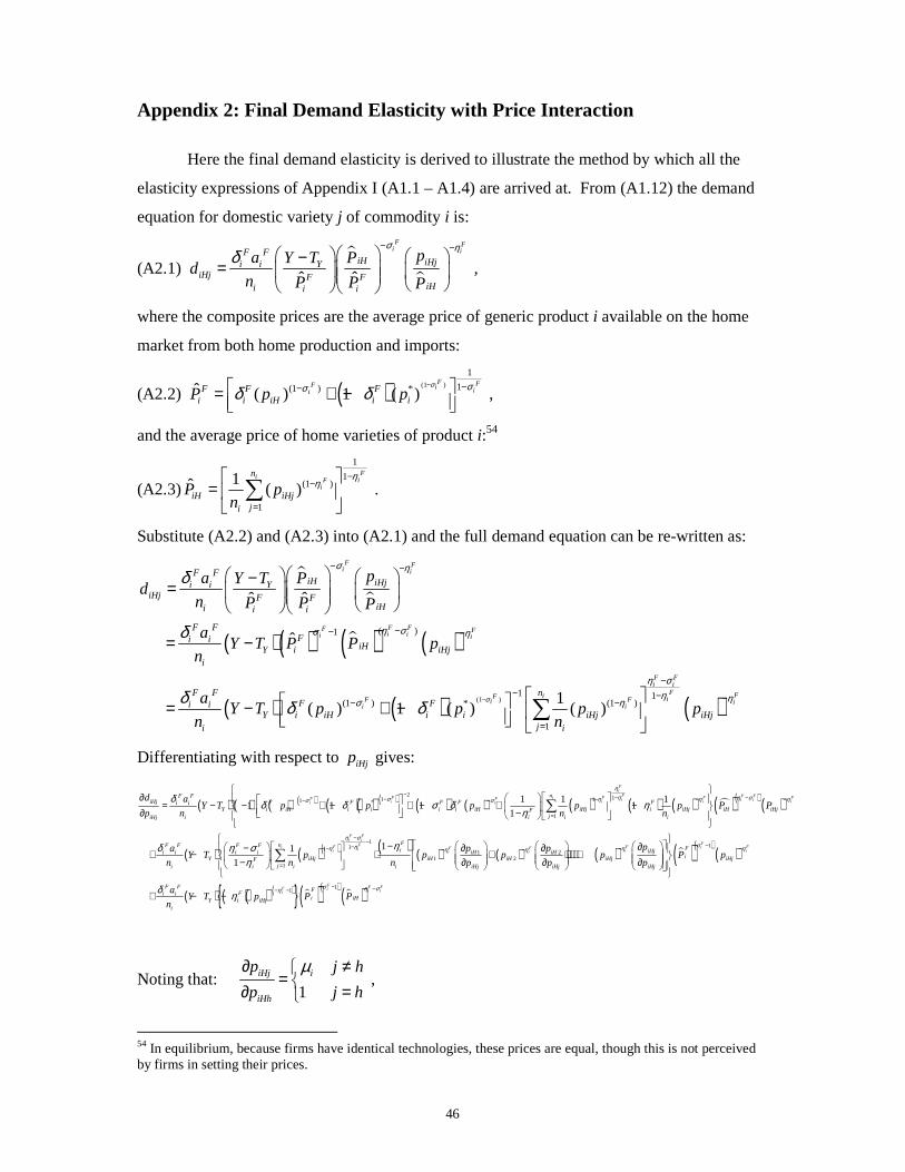
46
Appendix 2: Final Demand Elasticity with Price Interaction
Here the final demand elasticity is derived to illustrate the method by which all the
elasticity expressions of Appendix I (A1.1 – A1.4) are arrived at. From (A1.12) the demand
equation for domestic variety j of commodity i is:
(A2.1) �
�ˆ ˆ
F Fi iF F
iH iHji i YiHj F F
iHi i i
pa Y T Pd
n P P P
σ ηδ
− − −=
,
where the composite prices are the average price of generic product i available on the home
market from both home production and imports:
(A2.2) ( ) (1 )
1
1(1 ) *ˆ ( ) 1 ( )F FF i iiF F F
i i iH i iP p pσ σσδ δ
− −− = + −
,
and the average price of home varieties of product i:54
(A2.3)
1
1(1 )
1
1ˆ ( )Fi iF
i
n
iH iHjji
P pn
ηη
−−
=
= ∑ .
Substitute (A2.2) and (A2.3) into (A2.1) and the full demand equation can be re-written as:
�
�
( )( ) �( ) ( )
( ) ( ) (1 )
( )1
1 1(1 ) (1 )*
1
ˆ ˆ
ˆ
1( ) 1 ( ) ( )
F Fi i
F FF Fi ii i
F Fi i
FiF iF Fii i
F FiH iHji i Y
iHj F FiHi i i
F FFi i
iHY i iHji
nF FF Fi i
Y i iH i i iHjji i
pa Y T Pd
n P P P
aY T P P p
n
aY T p p p p
n n
σ
σ η
η σσ η
η ση
σ η
δ
δ
δ δ δ−
− −
−− −
−− −
− −
=
−=
= −
= − + − ∑ ( )
Fi
iHj
η−
Differentiating with respect to iHjp gives:
( ) ( ) ( )( ) ( )( )( ) ( ) ( ) ( ) ( ) ( ) �( )( ) ( )
( )
2 11 11 *
1
1
1 1 11 1 1 1
1
1
1
Fi
F F FF F F FiF F i i ii i i ii i
nF FiHj F F F F Fi i
Y i iH i i i i iH iHj i iHj iH iHjFjiHj i i i i
F F F Fi i i i
Y Fji i i
d aY T p p p p p P P
p n n n
aY T
n n
ηη η σσ η η ησ σδ δ δ σ δ η
η
δ η ση
− − −− − − −− −
=
=
∂ = − − + − ⋅ − ⋅ − ∂ −
−+ − −
∑
( )( ) ( ) ( ) ( ) ( ) �( )( )( )
( ) ( )( )( ){ } �( )( )�( )
1111
1 21 2
11
1F Fi i
FFF F Fi iF Fii i ii i
F FF i ii
Fn Fi iHjiH iHiiHj iH iH iHj iHj
i iHj iHj iHj
F F FFi i
i iHY i iHji
pp pp p p p P p
n p p p
aY T p P P
n
η σσηη η ηη η
σ ηη
η
δ η
− − −−− − −− −
− −− −
− ∂ ∂ ∂ ⋅ + + ⋅⋅ ⋅ + ∂ ∂ ∂
+ − −
∑
Fiσ
Noting that: 1
iHj i
iHh
p j h
p j h
µ∂ ≠= ∂ =
,
54 In equilibrium, because firms have identical technologies, these prices are equal, though this is not perceived by firms in setting their prices.
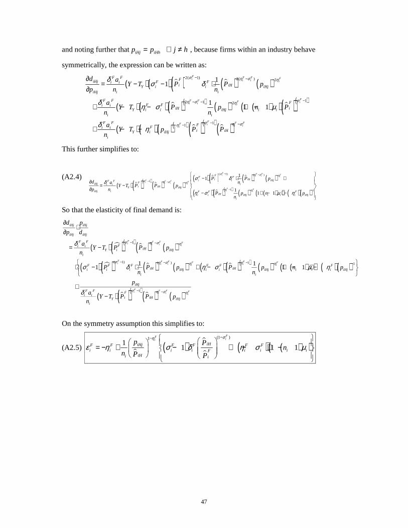
47
and noting further thatiHj iHhp p j h= ∀ ≠ , because firms within an industry behave
symmetrically, the expression can be written as:
( )( ) �( ) �( ) ( )
( )( ) �( )( ) ( ) ( )( ) �( )( )
( )( ) ( )( ) �( )( )�( )
2( 1) 2( ) 2
12 1 2
11
11
11 1
F F F Fi i i i
FF F F ii i i
F F FF i i ii
F F FiHj F Fi ii iHY i i iHj
iHj i i
F F FF Fi i
iH iY i i iHj i ii i
F F FFi i
i iHY i iHji
d aY T P P p
p n n
aY T P p n P
n n
aY T p P P
n
σ η σ η
ση σ η
σ η ση
δ σ δ
δ η σ µ
δ η
− − −
−− − −
− −− −
∂= − − ⋅
∂
+ − − + −
+ − −
This further simplifies to:
(A2.4) ( ) �( )( )
�( ) ( )( ) �( ) �( ) ( )
( ) �( )( ) ( ) ( )( ) ( )( )
( 1) ( )
1
1 1
11
11 1
F F F Fi i i i
F F F Fi i i i
F Fi i
FF F
i iHi i iHjF F FiHj ii ii iHY iHj
iHj i F F FiHi i iHj i i i iHj
i
P P pd na
Y T P P pp n
P p n pn
σ η σ η
σ η σ η
η η
σ δδ
η σ µ η
− − −
− − −
− − −
− ⋅ + ∂ = − ∂ − + − + −
So that the elasticity of final demand is:
( ) �( )( )�( ) ( )
( ) �( ) �( ) ( ) ( ) �( )( ) ( ) ( )( ) ( ) ( )
( ) �( )( )�( ) ( )
1
( 1) ( ) 1 1
1
1 11 1 1
F F F Fi i i i
F F F FF Fi i i ii i
F F F Fi i i i
iHj iHj
iHj iHj
F FFi i
iHY i iHji
F F F F F FiH iHi i i iHj i i iHj i i i iHj
i i
iHj
F F Fi i
i iHY iHji
d p
p d
aY T P P p
n
P P p P p n pn n
p
aY T P P p
n
σ η σ η
σ η σ ηη η
σ η σ η
δ
σ δ η σ µ η
δ
− − −
− − −− − −
− − −
∂⋅
∂
= −
⋅ − ⋅ + − + − + −
⋅−
On the symmetry assumption this simplifies to:
(A2.5) �
( )�
�( ) ( )( )
(1 )11
1 1 1
FFii
iHiHjF F F F F Fi i i i i i i iF
iHi i
p Pn
n P P
ση
ε η σ δ η σ µ−− = − + − + − + −
Recommended

![LECTURE #15: MICROECONOMICS CHAPTER 17 [Chapter 16 in 4th Edition] Oligopolies Game Theory Public Policy](https://img.pdfslide.us/doc/110x75/56649cf85503460f949c8676/lecture-15-microeconomics-chapter-17-chapter-16-in-4th-edition-oligopolies.jpg)