Sequence AlignmentCont’d
Sequence Alignment
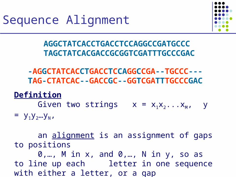
-AGGCTATCACCTGACCTCCAGGCCGA--TGCCC---TAG-CTATCAC--GACCGC--GGTCGATTTGCCCGAC
DefinitionGiven two strings x = x1x2...xM, y
= y1y2…yN,
an alignment is an assignment of gaps to positions
0,…, M in x, and 0,…, N in y, so as to line up each letter in one sequence with either a letter, or a gap
in the other sequence
AGGCTATCACCTGACCTCCAGGCCGATGCCCTAGCTATCACGACCGCGGTCGATTTGCCCGAC
Scoring Function
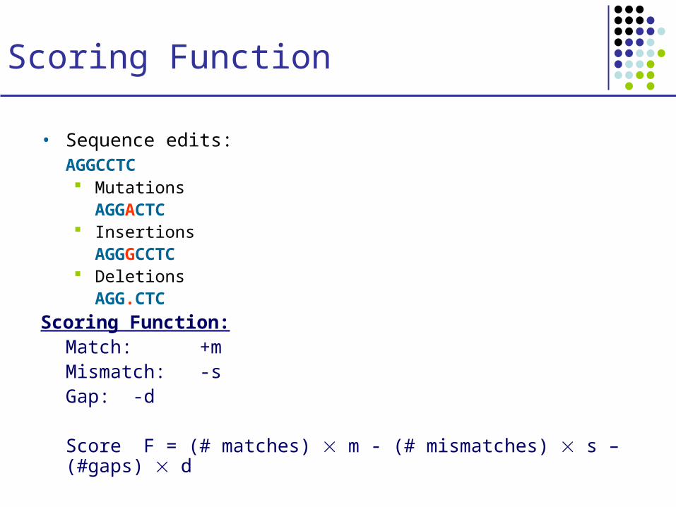
• Sequence edits:AGGCCTC
Mutations AGGACTC
InsertionsAGGGCCTC
DeletionsAGG.CTC
Scoring Function:Match: +mMismatch: -sGap: -d
Score F = (# matches) m - (# mismatches) s – (#gaps) d
The Needleman-Wunsch Algorithm
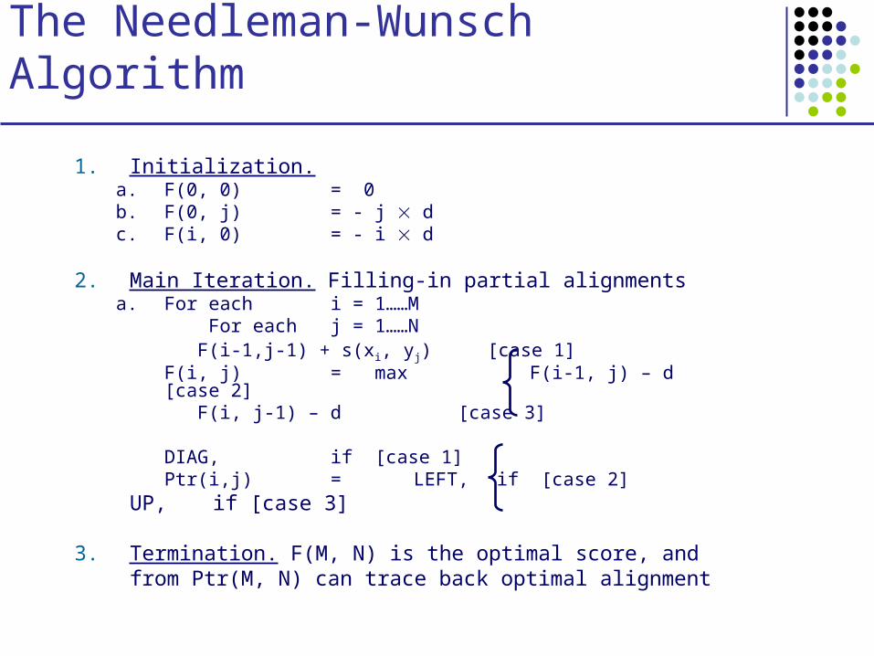
1. Initialization.a. F(0, 0) = 0b. F(0, j) = - j dc. F(i, 0) = - i d
2. Main Iteration. Filling-in partial alignmentsa. For each i = 1……M
For each j = 1……N F(i-1,j-1) + s(xi, yj)
[case 1]F(i, j) = max F(i-1, j) – d
[case 2] F(i, j-1) – d
[case 3]
DIAG, if [case 1]Ptr(i,j) = LEFT, if [case 2]
UP, if [case 3]
3. Termination. F(M, N) is the optimal score, andfrom Ptr(M, N) can trace back optimal alignment
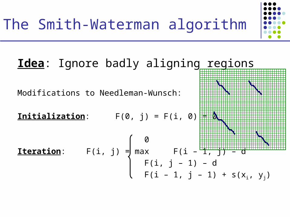
The Smith-Waterman algorithm
Idea: Ignore badly aligning regions
Modifications to Needleman-Wunsch:
Initialization: F(0, j) = F(i, 0) = 0
0
Iteration: F(i, j) = max F(i – 1, j) – d
F(i, j – 1) – d
F(i – 1, j – 1) + s(xi, yj)
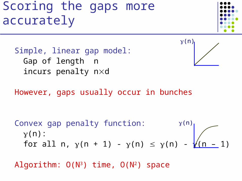
Scoring the gaps more accurately
Simple, linear gap model:Gap of length nincurs penalty nd
However, gaps usually occur in bunches
Convex gap penalty function:(n):for all n, (n + 1) - (n) (n) - (n – 1)
Algorithm: O(N3) time, O(N2) space
(n)
(n)
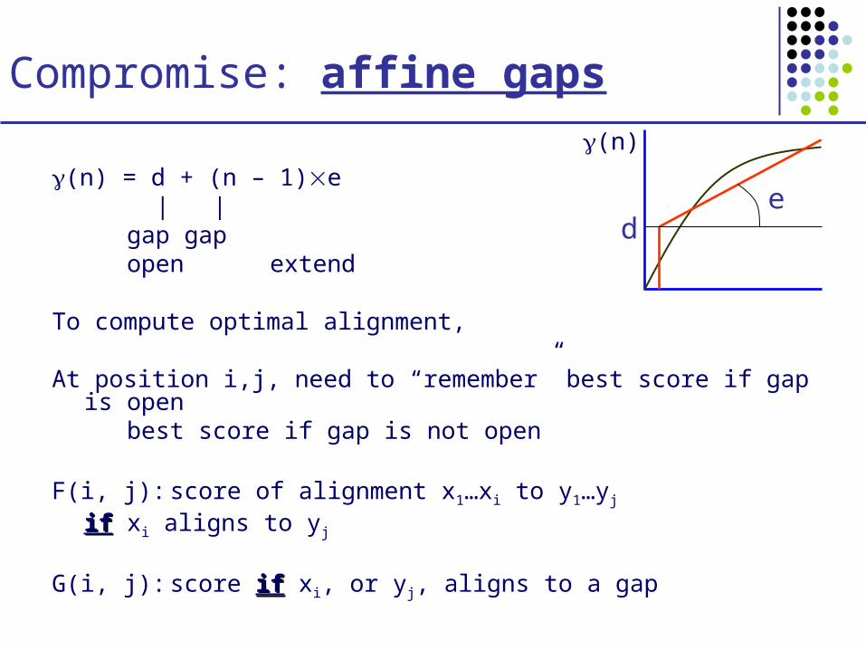
Compromise: affine gaps
(n) = d + (n – 1)e | | gap gap open extend
To compute optimal alignment,
At position i,j, need to “remember” best score if gap is open best score if gap is not open
F(i, j): score of alignment x1…xi to y1…yj
ifif xi aligns to yj
G(i, j): score ifif xi, or yj, aligns to a gap
de
(n)
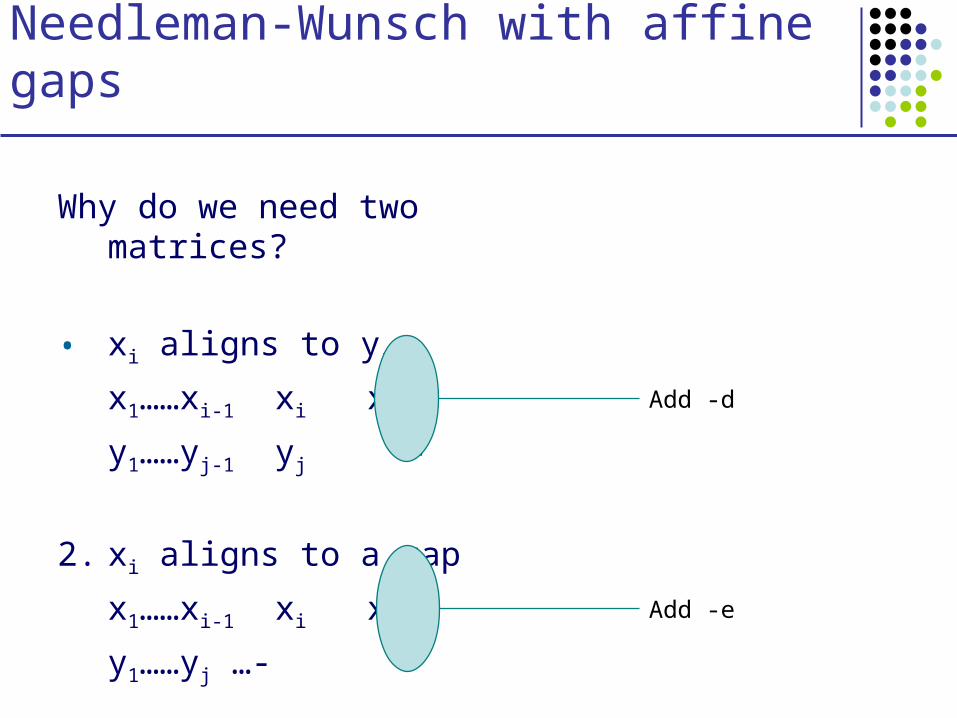
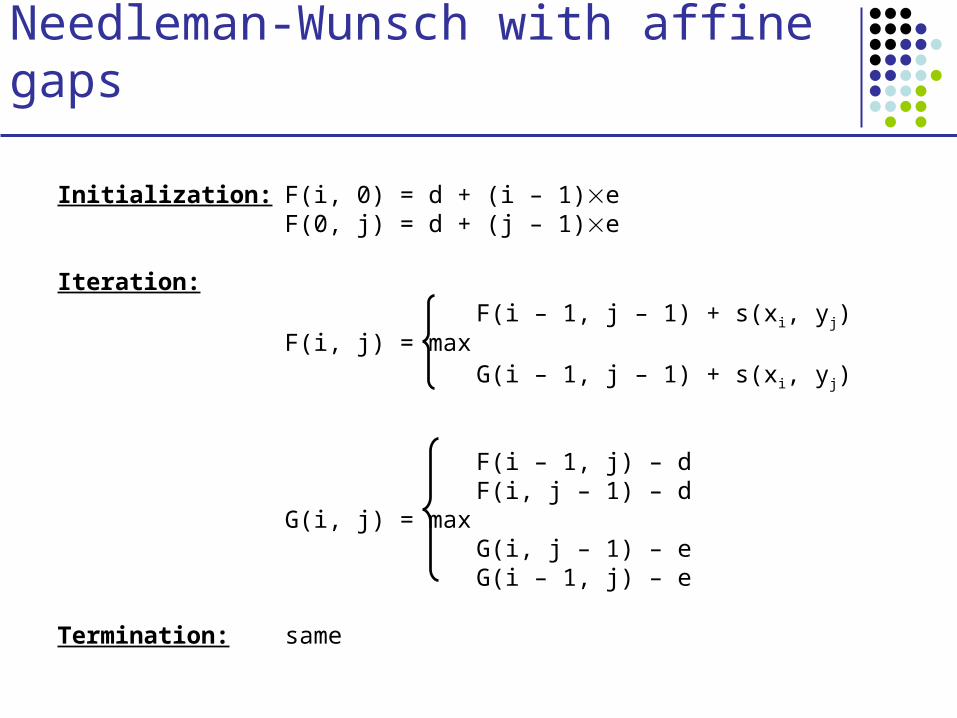
Needleman-Wunsch with affine gaps
Why do we need two matrices?
• xi aligns to yj
x1……xi-1 xi xi+1
y1……yj-1 yj -
2. xi aligns to a gap
x1……xi-1 xi xi+1
y1……yj …- -
Add -d
Add -e
Needleman-Wunsch with affine gaps
Initialization: F(i, 0) = d + (i – 1)eF(0, j) = d + (j – 1)e
Iteration:F(i – 1, j – 1) + s(xi, yj)
F(i, j) = maxG(i – 1, j – 1) + s(xi, yj)
F(i – 1, j) – d F(i, j – 1) – d
G(i, j) = max G(i, j – 1) – eG(i – 1, j) – e
Termination: same
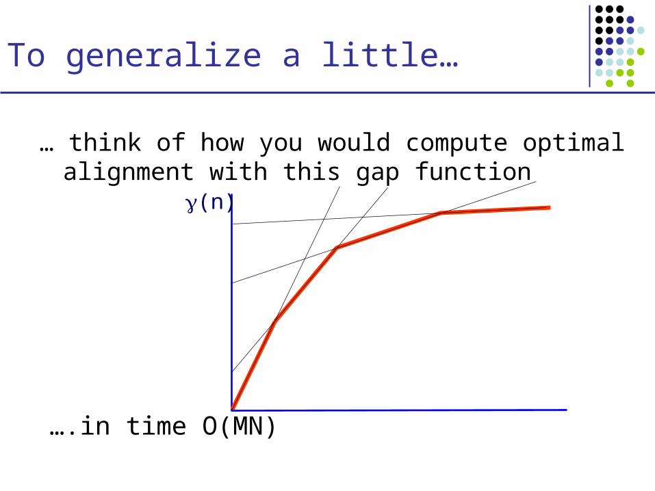
To generalize a little…
… think of how you would compute optimal alignment with this gap function
….in time O(MN)
(n)
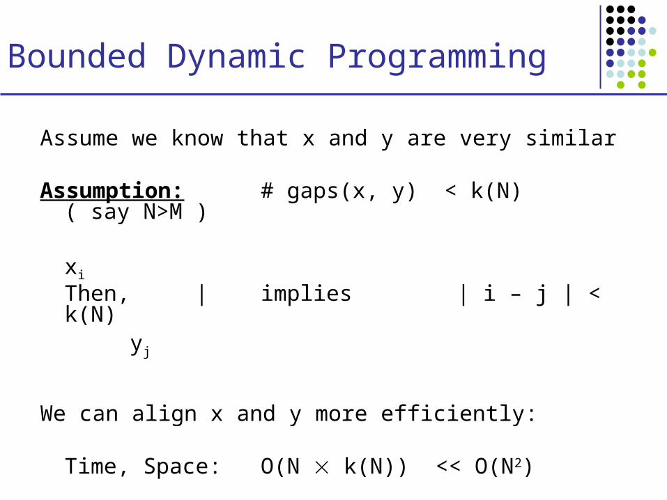
Bounded Dynamic Programming
Assume we know that x and y are very similar
Assumption: # gaps(x, y) < k(N) ( say N>M )
xi Then, | implies | i – j | < k(N)
yj
We can align x and y more efficiently:
Time, Space: O(N k(N)) << O(N2)
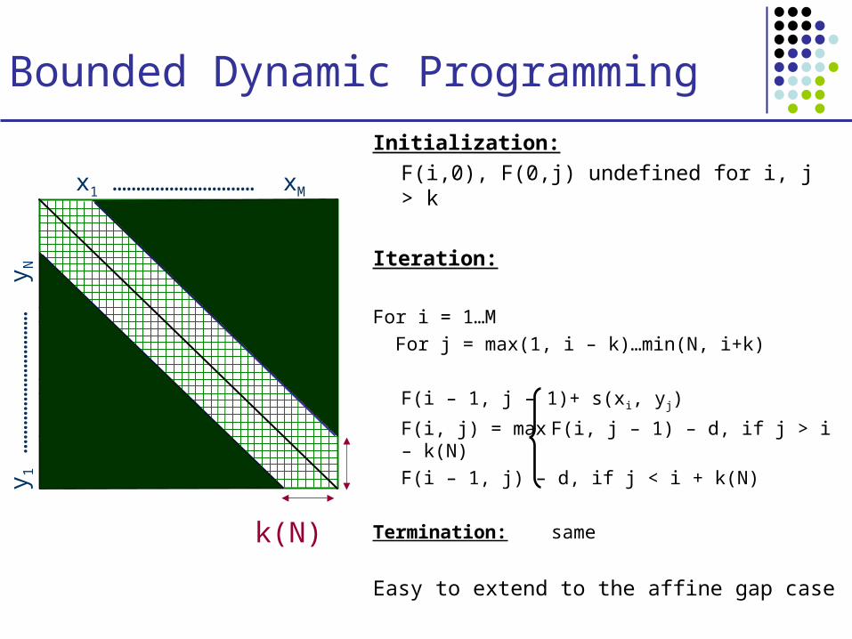
Bounded Dynamic Programming
Initialization:
F(i,0), F(0,j) undefined for i, j > k
Iteration:
For i = 1…M
For j = max(1, i – k)…min(N, i+k)
F(i – 1, j – 1)+ s(xi, yj)
F(i, j) = max F(i, j – 1) – d, if j > i – k(N)
F(i – 1, j) – d, if j < i + k(N)
Termination: same
Easy to extend to the affine gap case
x1 ………………………… xM
y1 …
……
……
……
……
…
yN
k(N)
Linear-Space Alignment
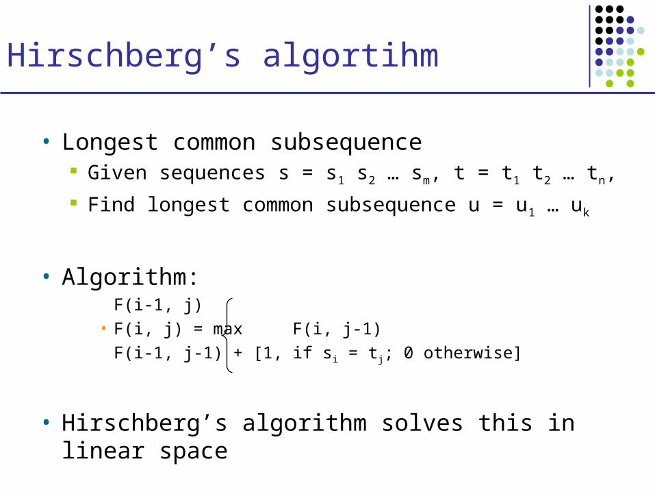
Hirschberg’s algortihm
• Longest common subsequence Given sequences s = s1 s2 … sm, t = t1 t2 … tn,
Find longest common subsequence u = u1 … uk
• Algorithm:F(i-1, j)
• F(i, j) = max F(i, j-1)
F(i-1, j-1) + [1, if si = tj; 0 otherwise]
• Hirschberg’s algorithm solves this in linear space
F(i,j)
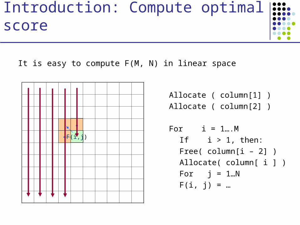
Introduction: Compute optimal score
It is easy to compute F(M, N) in linear space
Allocate ( column[1] )
Allocate ( column[2] )
For i = 1….M
If i > 1, then:
Free( column[i – 2] )
Allocate( column[ i ] )
For j = 1…N
F(i, j) = …
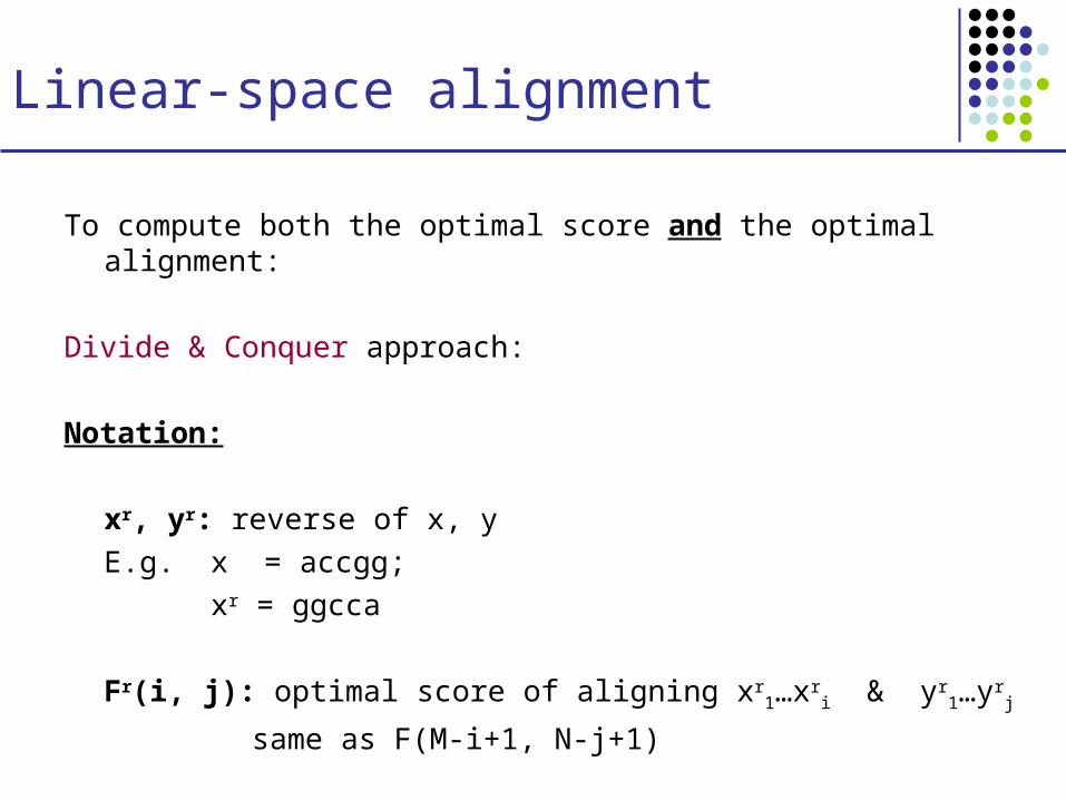
Linear-space alignment
To compute both the optimal score and the optimal alignment:
Divide & Conquer approach:
Notation:
xr, yr: reverse of x, y
E.g. x = accgg;
xr = ggcca
Fr(i, j): optimal score of aligning xr1…xr
i & yr1…yr
j
same as F(M-i+1, N-j+1)
Linear-space alignment
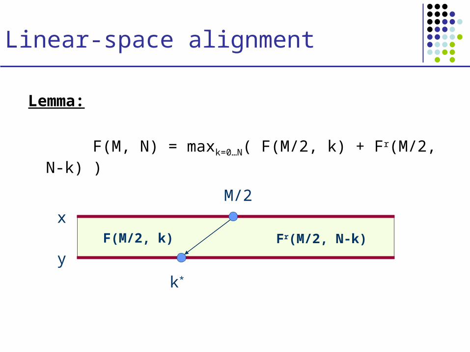
Lemma:
F(M, N) = maxk=0…N( F(M/2, k) + Fr(M/2, N-k) )
x
y
M/2
k*
F(M/2, k) Fr(M/2, N-k)
Linear-space alignment
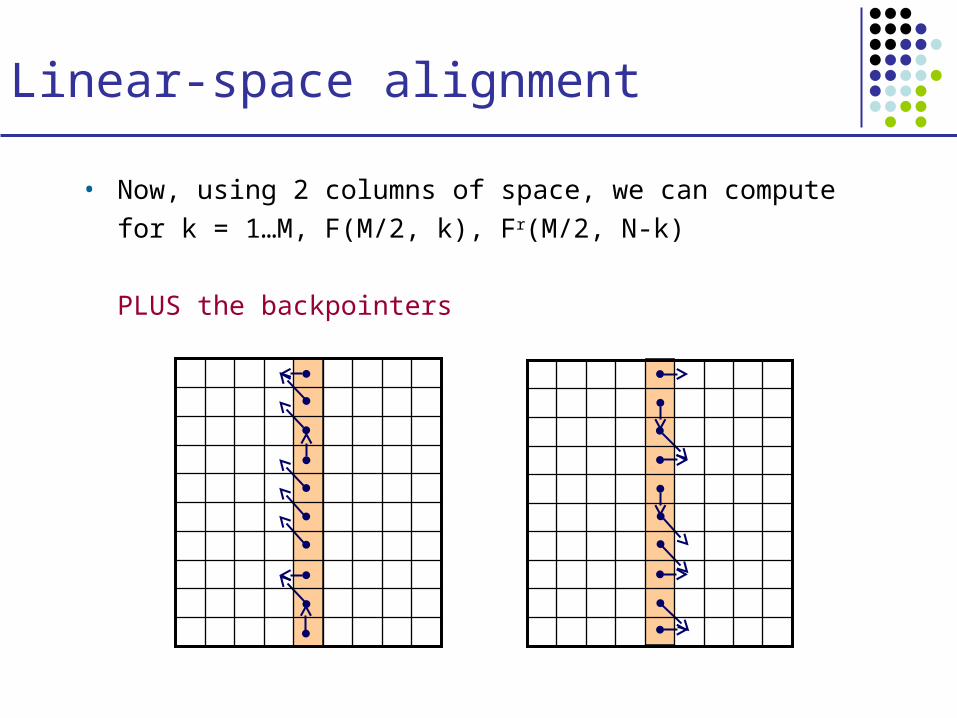
• Now, using 2 columns of space, we can compute
for k = 1…M, F(M/2, k), Fr(M/2, N-k)
PLUS the backpointers
Linear-space alignment
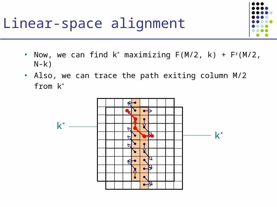
• Now, we can find k* maximizing F(M/2, k) + Fr(M/2, N-k)
• Also, we can trace the path exiting column M/2 from k*
k*
k*
Linear-space alignment
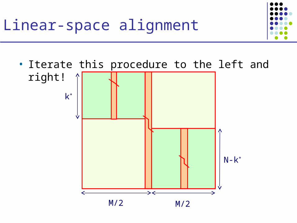
• Iterate this procedure to the left and right!
N-k*
M/2M/2
k*
Linear-space alignment
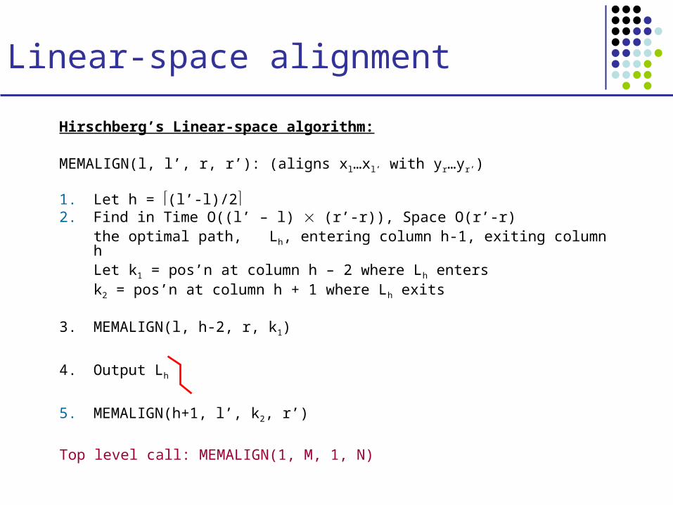
Hirschberg’s Linear-space algorithm:
MEMALIGN(l, l’, r, r’): (aligns xl…xl’ with yr…yr’)
1. Let h = (l’-l)/22. Find in Time O((l’ – l) (r’-r)), Space O(r’-r)
the optimal path, Lh, entering column h-1, exiting column hLet k1 = pos’n at column h – 2 where Lh enters
k2 = pos’n at column h + 1 where Lh exits
3. MEMALIGN(l, h-2, r, k1)
4. Output Lh
5. MEMALIGN(h+1, l’, k2, r’)
Top level call: MEMALIGN(1, M, 1, N)
Linear-space alignment
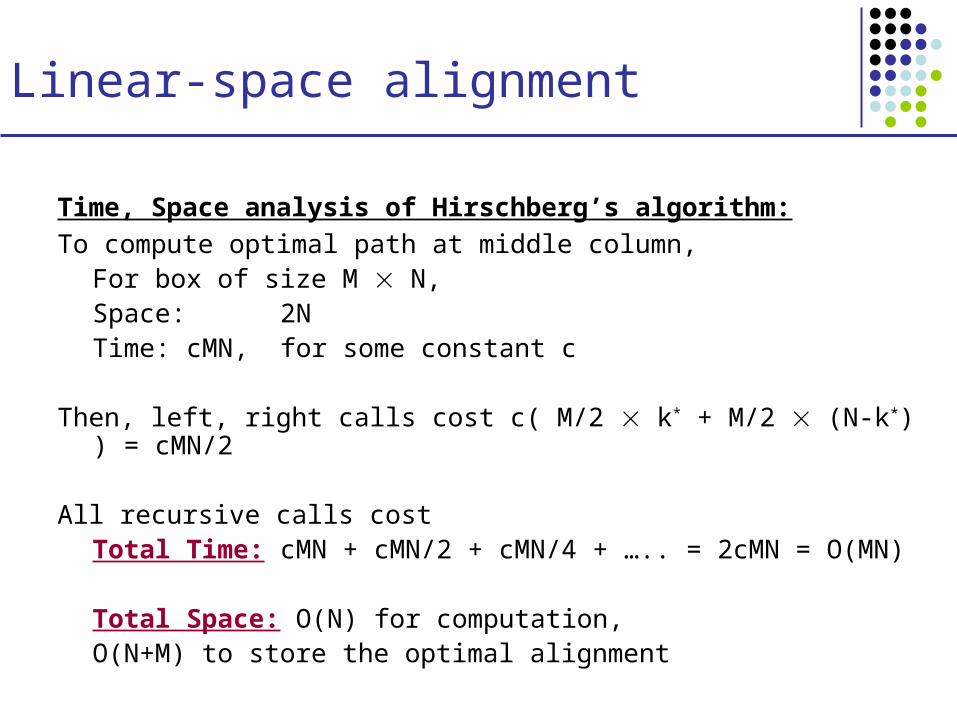
Time, Space analysis of Hirschberg’s algorithm: To compute optimal path at middle column,
For box of size M N,Space: 2NTime: cMN, for some constant c
Then, left, right calls cost c( M/2 k* + M/2 (N-k*) ) = cMN/2
All recursive calls cost Total Time: cMN + cMN/2 + cMN/4 + ….. = 2cMN = O(MN)
Total Space: O(N) for computation,O(N+M) to store the optimal alignment
The Four-Russian Algorithm
A useful speedup of Dynamic Programming
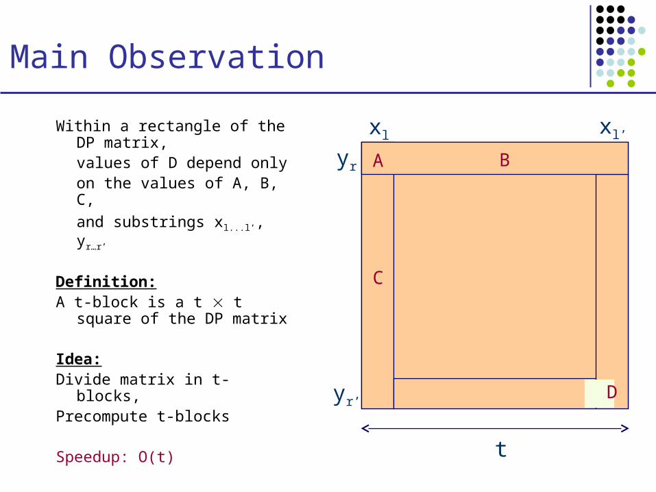
Main Observation
Within a rectangle of the DP matrix,values of D depend onlyon the values of A, B, C,
and substrings xl...l’, yr…r’
Definition: A t-block is a t t square of
the DP matrix
Idea: Divide matrix in t-blocks,Precompute t-blocks
Speedup: O(t)
A B
C
D
xl xl’
yr
yr’
t
The Four-Russian Algorithm
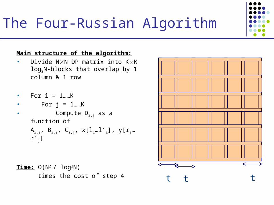
Main structure of the algorithm:
• Divide NN DP matrix into KK log2N-blocks that overlap by 1 column & 1 row
• For i = 1……K
• For j = 1……K
• Compute Di,j as a function of
Ai,j, Bi,j, Ci,j, x[li…l’i], y[rj…r’j]
Time: O(N2 / log2N)
times the cost of step 4t t t
The Four-Russian Algorithm
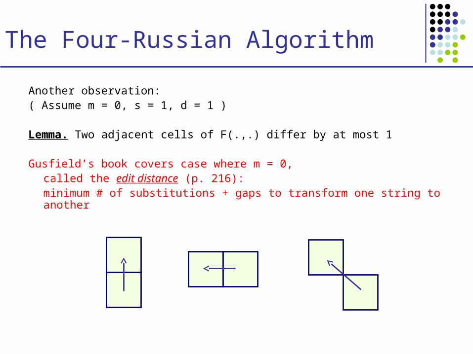
Another observation:( Assume m = 0, s = 1, d = 1 )
Lemma. Two adjacent cells of F(.,.) differ by at most 1
Gusfield’s book covers case where m = 0,called the edit distance (p. 216):minimum # of substitutions + gaps to transform one string to another
The Four-Russian Algorithm
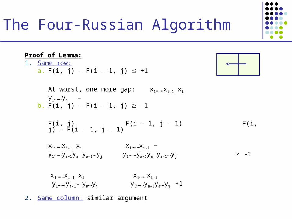
Proof of Lemma:1. Same row:
a. F(i, j) – F(i – 1, j) +1
At worst, one more gap: x1……xi-1 xi
y1……yj – b. F(i, j) – F(i – 1, j) -1
F(i, j) F(i – 1, j – 1) F(i, j) – F(i – 1, j – 1)
x1……xi-1 xi x1……xi-1 –y1……ya-1ya ya+1…yj y1……ya-1ya ya+1…yj -1
x1……xi-1 xi x1……xi-1
y1……ya-1– ya…yj y1……ya-1ya…yj +1
2. Same column: similar argument
The Four-Russian Algorithm
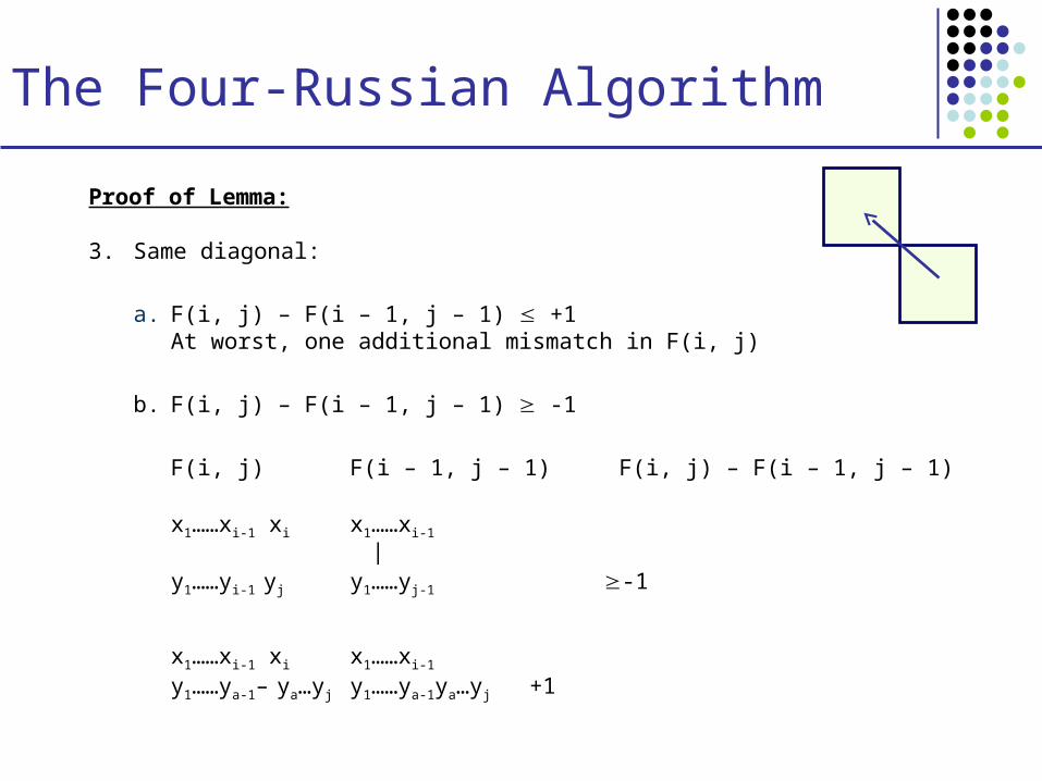
Proof of Lemma:
3. Same diagonal:
a. F(i, j) – F(i – 1, j – 1) +1At worst, one additional mismatch in F(i, j)
b. F(i, j) – F(i – 1, j – 1) -1
F(i, j) F(i – 1, j – 1) F(i, j) – F(i – 1, j – 1)
x1……xi-1 xi x1……xi-1
|y1……yi-1 yj y1……yj-1 -1
x1……xi-1 xi x1……xi-1
y1……ya-1– ya…yj y1……ya-1ya…yj +1
The Four-Russian Algorithm
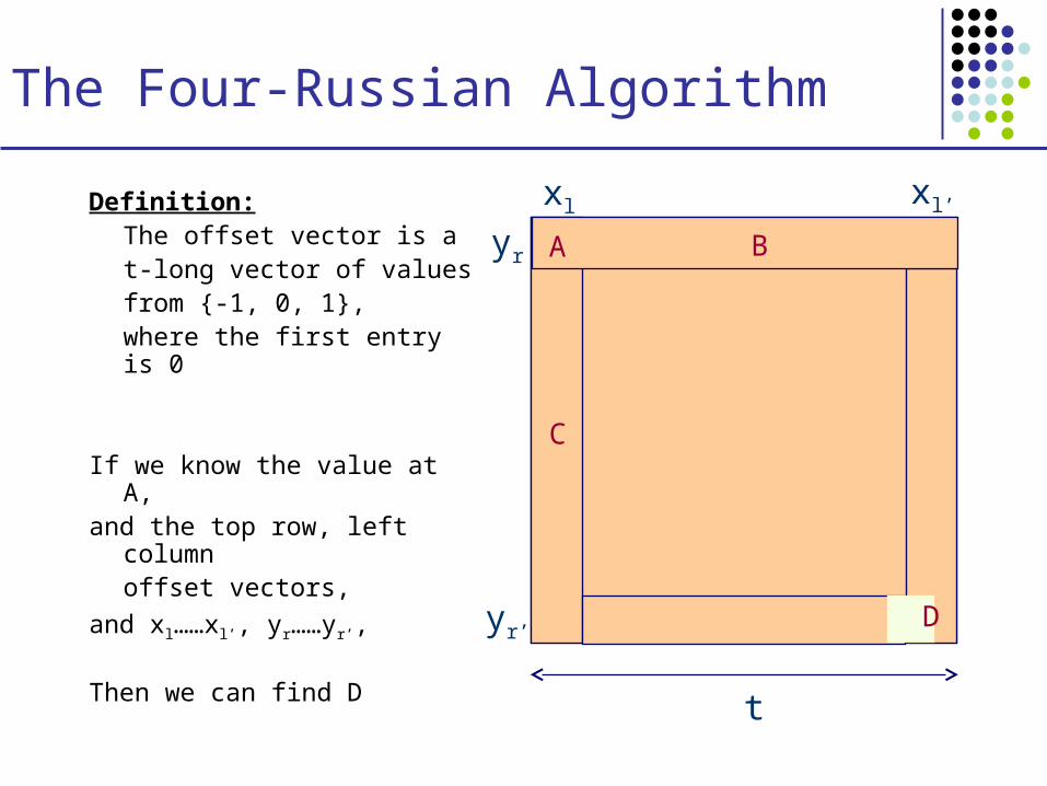
Definition:The offset vector is a t-long vector of values
from {-1, 0, 1}, where the first entry is 0
If we know the value at A,and the top row, left column
offset vectors,
and xl……xl’, yr……yr’,
Then we can find D
A B
C
D
xl xl’
yr
yr’
t
The Four-Russian Algorithm
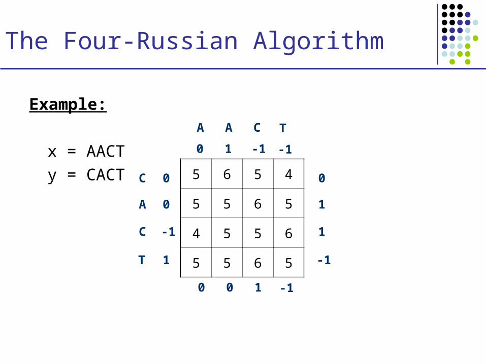
Example:
x = AACT
y = CACT 5 6 5 4
5 5 6 5
4 5 5 6
5 5 6 5
A A C T
C
A
C
T
0 1 -1 -1
0
0
-1
1
0 0 1 -1
0
1
1
-1

The Four-Russian Algorithm
Example:
x = AACT
y = CACT 1 2 1 0
1 1 2 1
0 1 1 2
1 1 2 1
A A C T
C
A
C
T
0 1 -1 -1
0
0
-1
1
0 0 1 -1
0
1
1
-1
The Four-Russian Algorithm
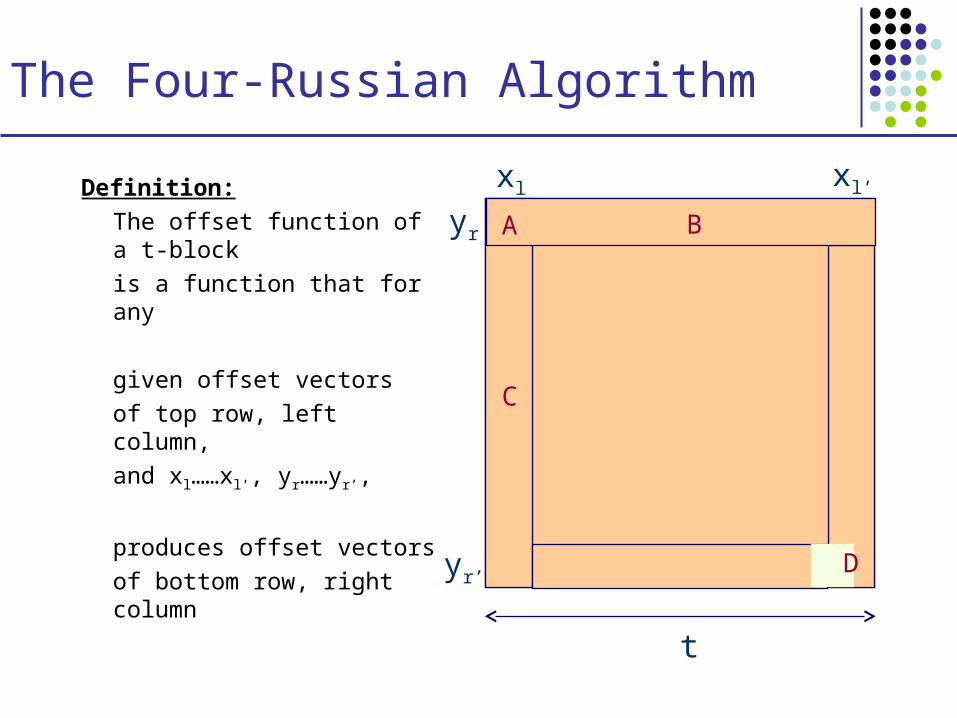
Definition:
The offset function of a t-block
is a function that for any
given offset vectors
of top row, left column,
and xl……xl’, yr……yr’,
produces offset vectors
of bottom row, right column
A B
C
D
xl xl’
yr
yr’
t
The Four-Russian Algorithm
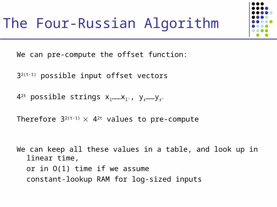
We can pre-compute the offset function:
32(t-1) possible input offset vectors
42t possible strings xl……xl’, yr……yr’
Therefore 32(t-1) 42t values to pre-compute
We can keep all these values in a table, and look up in linear time,
or in O(1) time if we assume
constant-lookup RAM for log-sized inputs
The Four-Russian Algorithm
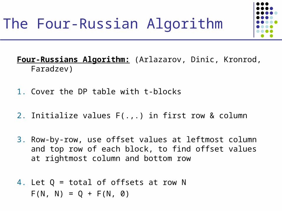
Four-Russians Algorithm: (Arlazarov, Dinic, Kronrod, Faradzev)
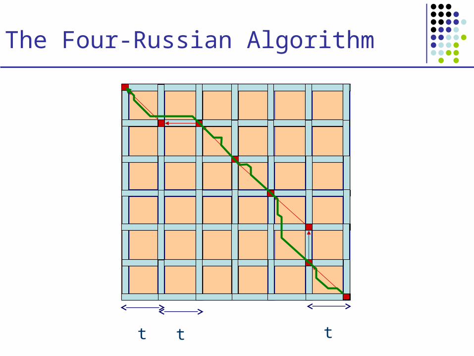
1. Cover the DP table with t-blocks
2. Initialize values F(.,.) in first row & column
3. Row-by-row, use offset values at leftmost column and top row of each block, to find offset values at rightmost column and bottom row
4. Let Q = total of offsets at row N
F(N, N) = Q + F(N, 0)
The Four-Russian Algorithm
t t t
Recommended

![Measuring Constructive Alignment: An Alignment Metric to … · computes the level of constructive alignment [3]. Constructive alignment is an outcome-based methodology developed](https://img.pdfslide.us/doc/110x75/5f0ec6317e708231d440df49/measuring-constructive-alignment-an-alignment-metric-to-computes-the-level-of-constructive.jpg)