Sensor Processing and Path Planning Frameworkfor a Search and Rescue UAV Network
by
Andrew BrownJonathan Estabrook
Brian Franklin
A Major Qualifying ProjectSubmitted to the Faculty
of theWORCESTER POLYTECHNIC INSTITUTEin partial fulfillment of the requirements for the
Degree of Bachelors of Sciencein
Electrical and Computer Engineeringand
Robotics Engineeringby
May 2012
APPROVED:
Dr. Alexander M. Wyglinski, Advisor
Dr. Taskin Padir, Co-Advisor
MQP-AW1-WND2 Keywords: UAV, Image Processing,SAR, Navigation, Framework
This report represents work of WPI undergraduate students submitted to the faculty asevidence of a degree requirement. WPI routinely publishes these reports on its web sitewithout editorial or peer review. For more information about the projects program at
WPI, see http://www.wpi.edu/Academics/Projects.
Abstract
Search and rescue operations are a costly endeavour. The advent of new technologies,
such as unmanned aerial vehicles, can decrease the cost of such operations and increase
rescue rates by finding the lost individual in a faster manner. However, the issue currently
faced is how to develop and deploy such a system comprised of multiple UAVs. This report
describes a framework which, through the use of modular components, provides for the
autonomous search and detection of a target with the flexibility to change hardware and
mission specific components at will. This framework integrates multi-agent path planning,
wireless communication and coordination, and on board sensor processing, fusing an FPGA,
DSP, and software platform for maximum flexibility with real time performance.
iii
Executive Summary
Each year in the United States, thousands of incidents occur resulting in the need
for massive search and rescue efforts to be launched. The brunt of these efforts is
undertaken by local law enforcement, the Coast Guard, and the National Park Service
supplemented by volunteers.
Budget cuts are the omnipresent reality of today’s economy. Search operations are
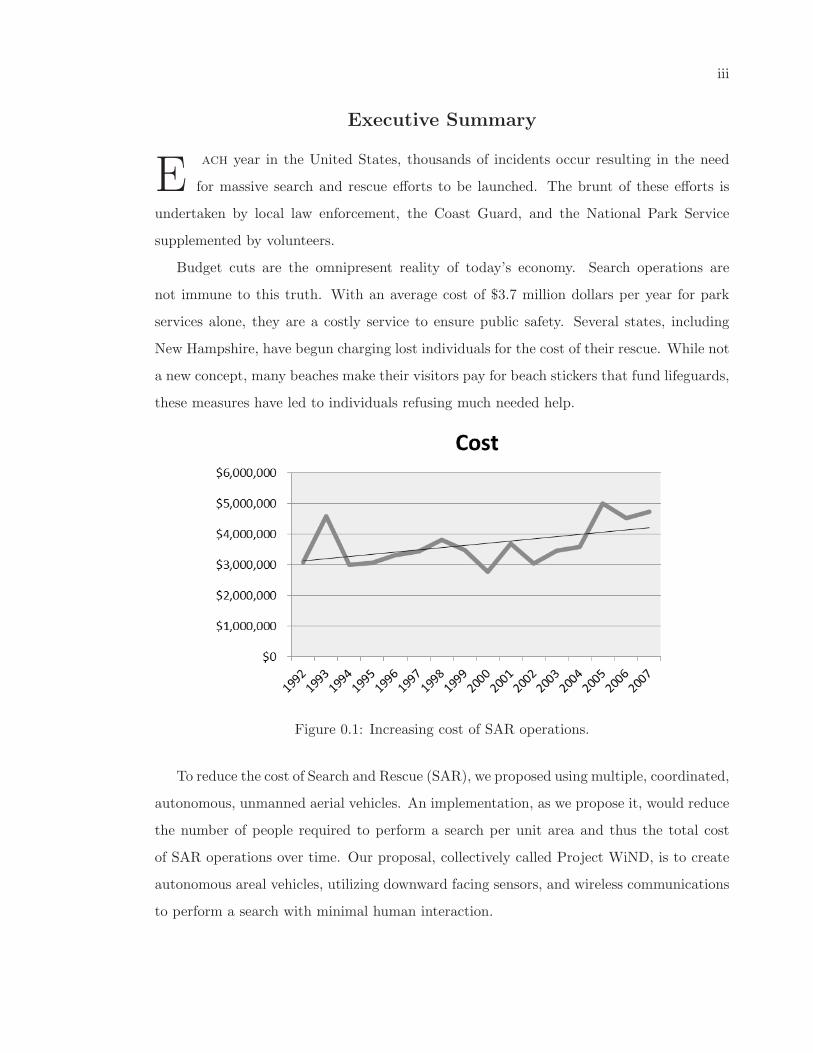
not immune to this truth. With an average cost of $3.7 million dollars per year for park
services alone, they are a costly service to ensure public safety. Several states, including
New Hampshire, have begun charging lost individuals for the cost of their rescue. While not
a new concept, many beaches make their visitors pay for beach stickers that fund lifeguards,
these measures have led to individuals refusing much needed help.
Figure 0.1: Increasing cost of SAR operations.
To reduce the cost of Search and Rescue (SAR), we proposed using multiple, coordinated,
autonomous, unmanned aerial vehicles. An implementation, as we propose it, would reduce
the number of people required to perform a search per unit area and thus the total cost
of SAR operations over time. Our proposal, collectively called Project WiND, is to create
autonomous areal vehicles, utilizing downward facing sensors, and wireless communications
to perform a search with minimal human interaction.
iv
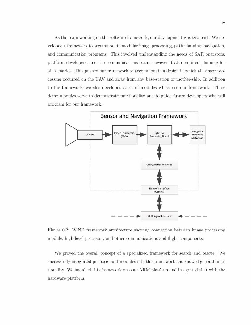
As the team working on the software framework, our development was two part. We de-
veloped a framework to accommodate modular image processing, path planning, navigation,
and communication programs. This involved understanding the needs of SAR operators,
platform developers, and the communications team, however it also required planning for
all scenarios. This pushed our framework to accommodate a design in which all sensor pro-
cessing occurred on the UAV and away from any base-station or mother-ship. In addition
to the framework, we also developed a set of modules which use our framework. These
demo modules serve to demonstrate functionality and to guide future developers who will
program for our framework.
Figure 0.2: WiND framework architecture showing connection between image processing
module, high level processor, and other communications and flight components.
We proved the overall concept of a specialized framework for search and rescue. We
successfully integrated purpose built modules into this framework and showed general func-
tionality. We installed this framework onto an ARM platform and integrated that with the
hardware platform.

v
We made significant headway in developing a search and rescue specific unmanned aerial
vehicle framework. This framework is open for developers to add functionality in the areas
of communications, image processing, and navigation. We hope that a future team can
finalize the framework and release it as a field-ready development platform.
vi
Contents
List of Figures viii
List of Tables xi
1 Introduction 11.1 Search and Rescue as a Public Service . . . . . . . . . . . . . . . . . . . . . 11.2 Cost of Search and Rescue . . . . . . . . . . . . . . . . . . . . . . . . . . . 21.3 The UAV Solution to SAR Operations . . . . . . . . . . . . . . . . . . . . . 51.4 A Gap in Current Research . . . . . . . . . . . . . . . . . . . . . . . . . . . 61.5 Proposed Approach . . . . . . . . . . . . . . . . . . . . . . . . . . . . . . . . 61.6 Project Organization and Contributions . . . . . . . . . . . . . . . . . . . . 91.7 Report Organization . . . . . . . . . . . . . . . . . . . . . . . . . . . . . . . 10
2 Prior Art 112.1 Path Planning . . . . . . . . . . . . . . . . . . . . . . . . . . . . . . . . . . 11
2.1.1 Search and Rescue Theory . . . . . . . . . . . . . . . . . . . . . . . . 112.1.2 AI Path Generation . . . . . . . . . . . . . . . . . . . . . . . . . . . 13
2.2 Image Processing . . . . . . . . . . . . . . . . . . . . . . . . . . . . . . . . . 152.3 Prior Integration Projects and Existing Frameworks . . . . . . . . . . . . . 182.4 Chapter Summary . . . . . . . . . . . . . . . . . . . . . . . . . . . . . . . . 20
3 Proposed Approach 213.1 Framework Architecture . . . . . . . . . . . . . . . . . . . . . . . . . . . . . 223.2 Path Planning . . . . . . . . . . . . . . . . . . . . . . . . . . . . . . . . . . 233.3 Image Processing . . . . . . . . . . . . . . . . . . . . . . . . . . . . . . . . . 26
3.3.1 FPGA-DSP . . . . . . . . . . . . . . . . . . . . . . . . . . . . . . . . 263.3.2 CPU-GPU . . . . . . . . . . . . . . . . . . . . . . . . . . . . . . . . 28
3.4 Framework Considerations . . . . . . . . . . . . . . . . . . . . . . . . . . . . 283.5 Chapter Summary . . . . . . . . . . . . . . . . . . . . . . . . . . . . . . . . 29
4 Implementation 304.1 System Architecture . . . . . . . . . . . . . . . . . . . . . . . . . . . . . . . 314.2 Navigation Module Development . . . . . . . . . . . . . . . . . . . . . . . . 32
4.2.1 Hardware Choice . . . . . . . . . . . . . . . . . . . . . . . . . . . . . 32
vii
4.2.2 Path Planning Development . . . . . . . . . . . . . . . . . . . . . . . 354.2.3 Testing Procedure . . . . . . . . . . . . . . . . . . . . . . . . . . . . 41
4.3 Communications Formatting . . . . . . . . . . . . . . . . . . . . . . . . . . 434.4 Image Processing Development . . . . . . . . . . . . . . . . . . . . . . . . . 44
4.4.1 Hardware Choice . . . . . . . . . . . . . . . . . . . . . . . . . . . . . 444.4.2 Development . . . . . . . . . . . . . . . . . . . . . . . . . . . . . . . 474.4.3 Testing Procedure . . . . . . . . . . . . . . . . . . . . . . . . . . . . 52
4.5 Chapter Summary . . . . . . . . . . . . . . . . . . . . . . . . . . . . . . . . 54
5 Experimental Results 565.1 Framework . . . . . . . . . . . . . . . . . . . . . . . . . . . . . . . . . . . . 565.2 Image Processing . . . . . . . . . . . . . . . . . . . . . . . . . . . . . . . . . 58
5.2.1 Data Reduction . . . . . . . . . . . . . . . . . . . . . . . . . . . . . . 585.2.2 Algorithm Effectiveness . . . . . . . . . . . . . . . . . . . . . . . . . 595.2.3 Hardware Implementation . . . . . . . . . . . . . . . . . . . . . . . . 615.2.4 Runtime Benchmark . . . . . . . . . . . . . . . . . . . . . . . . . . . 61
5.3 Path Planning . . . . . . . . . . . . . . . . . . . . . . . . . . . . . . . . . . 625.4 Network Interface Layer . . . . . . . . . . . . . . . . . . . . . . . . . . . . . 655.5 Development Platforms . . . . . . . . . . . . . . . . . . . . . . . . . . . . . 67
5.5.1 Development Environment Setup . . . . . . . . . . . . . . . . . . . . 675.5.2 AI Testing Environment . . . . . . . . . . . . . . . . . . . . . . . . . 71
5.6 Chapter Summary . . . . . . . . . . . . . . . . . . . . . . . . . . . . . . . . 71
6 Conclusion 726.1 Future Work . . . . . . . . . . . . . . . . . . . . . . . . . . . . . . . . . . . 73
A Glossary 75
B Hardware Specifications 77
C AI Path Planning Code 81
D Framework Outline 115
E FPGA Image Processing Description 164
F Simulink Image Processing 185
Bibliography 196
viii
List of Figures
0.1 Increasing cost of SAR operations. . . . . . . . . . . . . . . . . . . . . . . . iii0.2 WiND framework architecture showing connection between image processing
module, high level processor, and other communications and flight compo-nents. . . . . . . . . . . . . . . . . . . . . . . . . . . . . . . . . . . . . . . . iv
1.1 Coast Guard Rescue Personnel during Hurricane Katrina [1] . . . . . . . . . 21.2 Increasing cost of SAR operations since 1992. . . . . . . . . . . . . . . . . . 31.3 The MQ-1 Predator Unmanned Aircraft, an Unmanned Aerial Vehicle re-
quiring multiple operators[2] . . . . . . . . . . . . . . . . . . . . . . . . . . . 41.4 Snapshot of the ground control station during a dry run of a Brigham Young
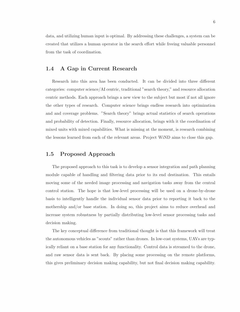
University WiSAR UAV. This UAV requires many human operators [3]. . . 51.5 Project WiND concept art showing many an Unmanned Aerial Vehicles op-
erating in a coordinated operation. Each utilizes downward looking sensorsand wireless communications. . . . . . . . . . . . . . . . . . . . . . . . . . . 7
1.6 WiND framework architecture showing connection between image processingmodule, high level processor, and other communications and flight compo-nents. . . . . . . . . . . . . . . . . . . . . . . . . . . . . . . . . . . . . . . . 8
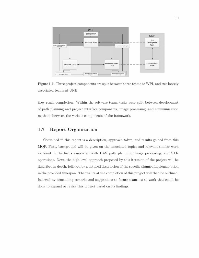
1.7 Three project components are split between three teams at WPI, and twoloosely associated teams at UNH. . . . . . . . . . . . . . . . . . . . . . . . 10
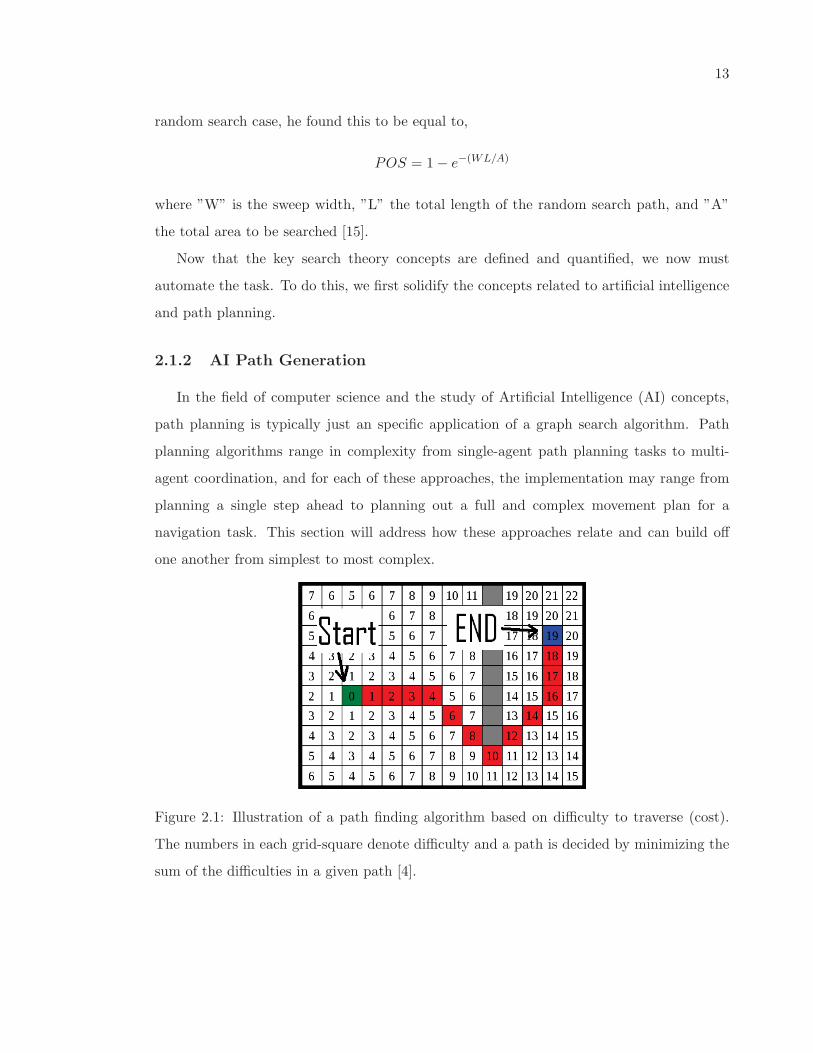
2.1 Illustration of a path finding algorithm based on difficulty to traverse (cost).The numbers in each grid-square denote difficulty and a path is decided byminimizing the sum of the difficulties in a given path [4]. . . . . . . . . . . . 13
2.2 Example of travelling salesman algorithm optimizing travel between N pointsfor shortest possible distance. Each iteration of this algorithm reduces thenumber of possible paths [5]. . . . . . . . . . . . . . . . . . . . . . . . . . . 14
2.3 Example of a blob detection algorithm running in MATLAB . . . . . . . . . 172.4 An FPGA and DSP Based, modular image processing system . . . . . . . . 182.5 MIT UAV architecture showing separation of aircraft control system and
path planning system . . . . . . . . . . . . . . . . . . . . . . . . . . . . . . 20
3.1 The proposed framework architecture, with interchangeable navigation andimage processing modules. . . . . . . . . . . . . . . . . . . . . . . . . . . . . 22
ix
3.2 Command and sensor inputs provide data for processing and waypoint gen-eration in the path planning module, which will then send planned waypointsto the autopilot hardware. . . . . . . . . . . . . . . . . . . . . . . . . . . . . 24
3.3 Comparison of image processing algorithms on FPGA, GPU, CPU [6] . . . 27
4.1 Final framework architecture showing connection between image processingmodule, high level processor, and other communications and flight compo-nents. . . . . . . . . . . . . . . . . . . . . . . . . . . . . . . . . . . . . . . . 31
4.2 High Level Processor Module (PandaBoard) . . . . . . . . . . . . . . . . . . 344.3 Hexagonal cells provide higher edge-crossing options than square grid cells. 364.4 A 30-degree-skewed Cartesian coordinate system provides uniform conversion
between local and global coordinate references. . . . . . . . . . . . . . . . . 374.5 Multi-point navigation to the nearest unvisited cell or nearest highest proba-
bility cell is performed using the A* algorithm. This provides path planningcapability around restricted regions. . . . . . . . . . . . . . . . . . . . . . . 38
4.6 A spiral or sweep search can be performed on any uniform grid by choosingthe next unvisited cell with a minimum distance to the sweep origin. . . . . 39
4.7 Path planning algorithms can be called in a cascaded manner behind a singleaccess point. This allows easy reconfiguration of the decision process. . . . . 39
4.8 Library class structure divides search grid data and utility data types behinda single access class. . . . . . . . . . . . . . . . . . . . . . . . . . . . . . . . 40
4.9 Cascaded navigation algorithms provide a robust and progressive decision-making process. . . . . . . . . . . . . . . . . . . . . . . . . . . . . . . . . . . 41
4.10 Signal Diagram showing the interfaces between different subsystems in theWiND Framework . . . . . . . . . . . . . . . . . . . . . . . . . . . . . . . . 42
4.11 JSON provides a more compact representation of data than XML. . . . . . 434.12 Spartan-6 LX9 Microboard . . . . . . . . . . . . . . . . . . . . . . . . . . . 454.13 Calculation of person size (in pixels) based on altitude and FOV [7] . . . . 464.14 Sony Block Camera[8] . . . . . . . . . . . . . . . . . . . . . . . . . . . . . . 474.15 A successive and independent, modular image processing algorithm we de-
veloped for testing our platform. . . . . . . . . . . . . . . . . . . . . . . . . 484.16 Simulink implementation of our custom image processing algorithm showing
manual adjustments. This easily adjustable model was used to fine-tune thealgorithm. . . . . . . . . . . . . . . . . . . . . . . . . . . . . . . . . . . . . . 50
4.17 Simulink implementation of the “Mean Deviation” block showing the algo-rithm chosen to define usual versus unusual pixels. . . . . . . . . . . . . . . 51
4.18 Block diagram showing dataflow for the HDL component of the image pro-cessing system. The outlined section labeled “Demo Module” shows theapplication specific blocks. . . . . . . . . . . . . . . . . . . . . . . . . . . . . 52
4.19 The team attempted to obtain aerial footage(See Right) via kite(see Left) . 534.20 The 16 different sample images above represent four altitudes and four dif-
ferent terrains. Arrows show the location of the person in each image . . . . 54
5.1 The initial network application interface, shown with a simulated flight path,message prompt, and configuration interface. . . . . . . . . . . . . . . . . . 57
x
5.2 Image processing algorithm run simulated forest setting at 100 ft . . . . . . 585.3 The main image is divided into ten smaller images based on objects detected
for transmission . . . . . . . . . . . . . . . . . . . . . . . . . . . . . . . . . . 595.4 Graph showing algorithm effectiveness over different terrains. . . . . . . . . 605.5 Image processing algorithm; from camera in, to heat map generation, binary
image filtering, to blob detection. . . . . . . . . . . . . . . . . . . . . . . . . 625.6 The web interface, configured to dump waypoints to the information console
for export. . . . . . . . . . . . . . . . . . . . . . . . . . . . . . . . . . . . . . 645.7 The autopilot control software running a hardware-in-the-loop simulation of
the waypoint sequence generated from the path planning module. . . . . . . 655.8 The web display allows usage and concurrent data reporting on any mobile
or PC platform with a standard web browser. . . . . . . . . . . . . . . . . . 665.9 Early PandaBoard testing configuration showing image capture capability
and networked VNC display. . . . . . . . . . . . . . . . . . . . . . . . . . . 685.10 VM Development Environment. . . . . . . . . . . . . . . . . . . . . . . . . . 70
F.1 Simulink implementation of our custom image processing algorithm showingmanual adjustments. This easily adjustable model was used to fine-tune thealgorithm. . . . . . . . . . . . . . . . . . . . . . . . . . . . . . . . . . . . . . 186
F.2 Simulink implementation of the “Mean Deviation” block showing the algo-rithm chosen to define usual versus unusual pixels. . . . . . . . . . . . . . . 187
xi
List of Tables
2.1 Comparison of SAR before and after the introduction of Search Theory [9] . 122.2 Greedy search chooses the next best option, not considering future steps in
a search task. . . . . . . . . . . . . . . . . . . . . . . . . . . . . . . . . . . . 14
5.1 Comparison of path planning resource usage on different platforms duringnavigation and map generation. For purposes of benchmarking, maps gener-ated had a cell radius of 10m and a grid radius of 50km. . . . . . . . . . . . 63
B.1 AI Hardware Choice Specification Comparison . . . . . . . . . . . . . . . . 79B.2 Image Processing Hardware Choice Specification Comparison . . . . . . . . 80
1
Chapter 1
Introduction
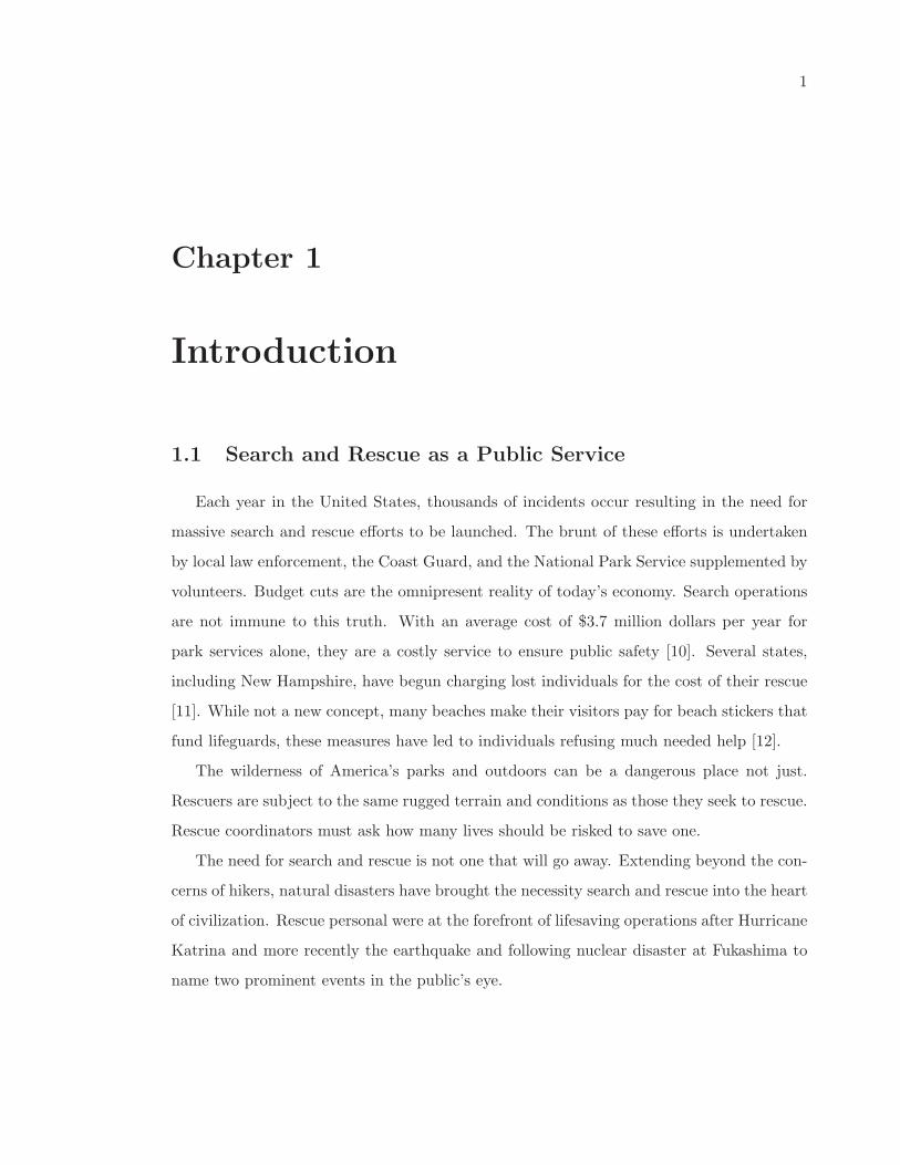
1.1 Search and Rescue as a Public Service
Each year in the United States, thousands of incidents occur resulting in the need for
massive search and rescue efforts to be launched. The brunt of these efforts is undertaken
by local law enforcement, the Coast Guard, and the National Park Service supplemented by
volunteers. Budget cuts are the omnipresent reality of today’s economy. Search operations
are not immune to this truth. With an average cost of $3.7 million dollars per year for
park services alone, they are a costly service to ensure public safety [10]. Several states,
including New Hampshire, have begun charging lost individuals for the cost of their rescue
[11]. While not a new concept, many beaches make their visitors pay for beach stickers that
fund lifeguards, these measures have led to individuals refusing much needed help [12].
The wilderness of America’s parks and outdoors can be a dangerous place not just.
Rescuers are subject to the same rugged terrain and conditions as those they seek to rescue.
Rescue coordinators must ask how many lives should be risked to save one.
The need for search and rescue is not one that will go away. Extending beyond the con-
cerns of hikers, natural disasters have brought the necessity search and rescue into the heart
of civilization. Rescue personal were at the forefront of lifesaving operations after Hurricane
Katrina and more recently the earthquake and following nuclear disaster at Fukashima to
name two prominent events in the public’s eye.
2
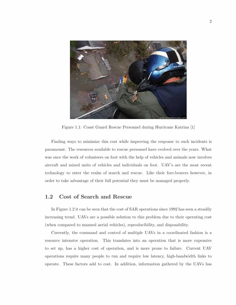
Figure 1.1: Coast Guard Rescue Personnel during Hurricane Katrina [1]
Finding ways to minimize this cost while improving the response to such incidents is
paramount. The resources available to rescue personnel have evolved over the years. What
was once the work of volunteers on foot with the help of vehicles and animals now involves
aircraft and mixed units of vehicles and individuals on foot. UAV’s are the most recent
technology to enter the realm of search and rescue. Like their fore-bearers however, in
order to take advantage of their full potential they must be managed properly.
1.2 Cost of Search and Rescue
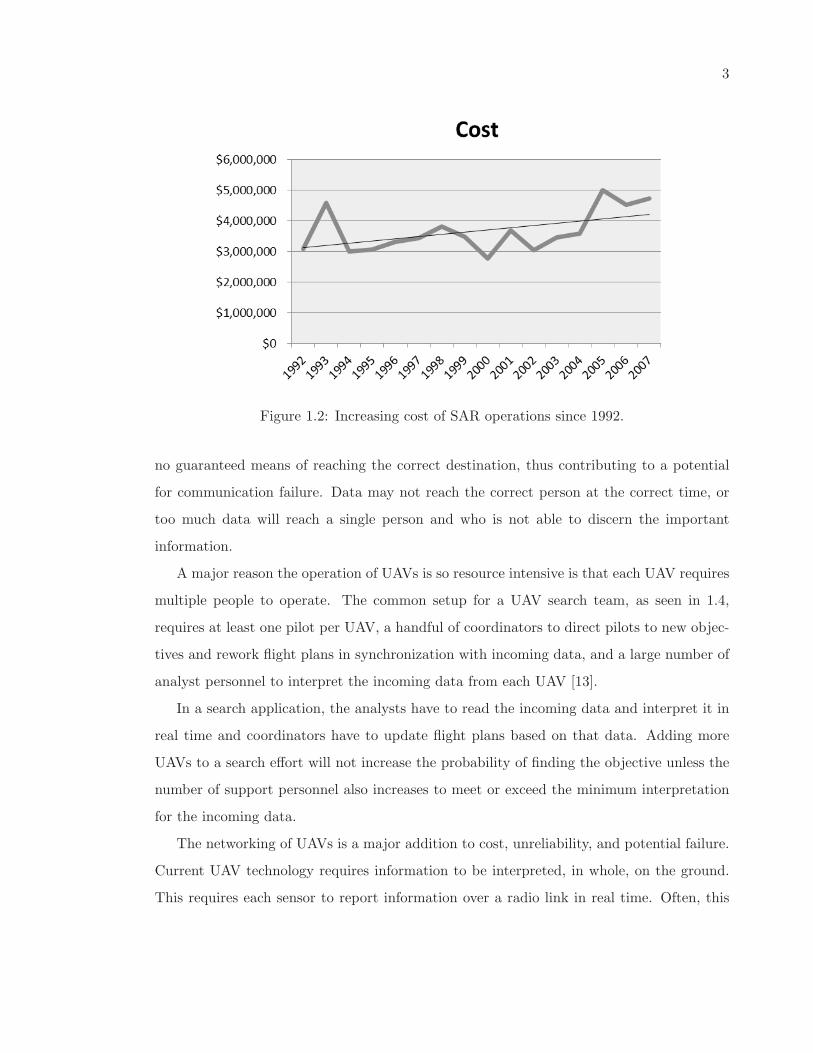
In Figure 1.2 it can be seen that the cost of SAR operations since 1992 has seen a steadily
increasing trend. UAVs are a possible solution to this problem due to their operating cost
(when compared to manned aerial vehicles), reproducibility, and disposability.
Currently, the command and control of multiple UAVs in a coordinated fashion is a
resource intensive operation. This translates into an operation that is more expensive
to set up, has a higher cost of operation, and is more prone to failure. Current UAV
operations require many people to run and require low latency, high-bandwidth links to
operate. These factors add to cost. In addition, information gathered by the UAVs has
3
Figure 1.2: Increasing cost of SAR operations since 1992.
no guaranteed means of reaching the correct destination, thus contributing to a potential
for communication failure. Data may not reach the correct person at the correct time, or
too much data will reach a single person and who is not able to discern the important
information.
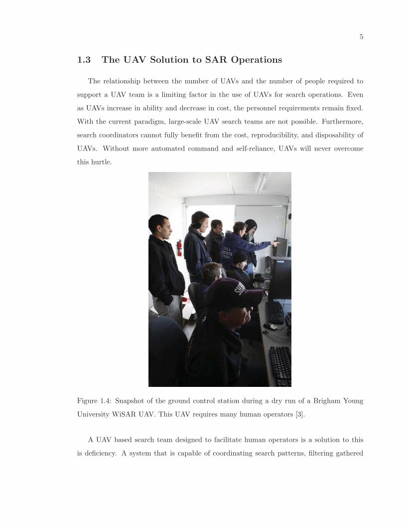
A major reason the operation of UAVs is so resource intensive is that each UAV requires
multiple people to operate. The common setup for a UAV search team, as seen in 1.4,
requires at least one pilot per UAV, a handful of coordinators to direct pilots to new objec-
tives and rework flight plans in synchronization with incoming data, and a large number of
analyst personnel to interpret the incoming data from each UAV [13].
In a search application, the analysts have to read the incoming data and interpret it in
real time and coordinators have to update flight plans based on that data. Adding more
UAVs to a search effort will not increase the probability of finding the objective unless the
number of support personnel also increases to meet or exceed the minimum interpretation
for the incoming data.
The networking of UAVs is a major addition to cost, unreliability, and potential failure.
Current UAV technology requires information to be interpreted, in whole, on the ground.
This requires each sensor to report information over a radio link in real time. Often, this
4
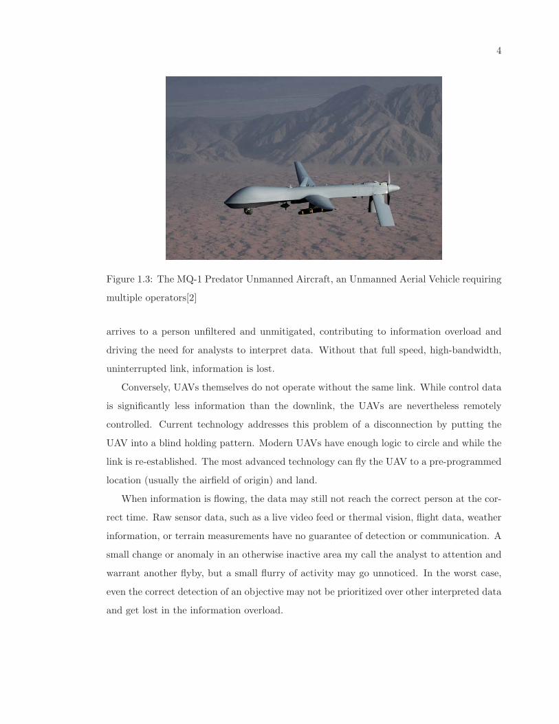
Figure 1.3: The MQ-1 Predator Unmanned Aircraft, an Unmanned Aerial Vehicle requiring
multiple operators[2]
arrives to a person unfiltered and unmitigated, contributing to information overload and
driving the need for analysts to interpret data. Without that full speed, high-bandwidth,
uninterrupted link, information is lost.
Conversely, UAVs themselves do not operate without the same link. While control data
is significantly less information than the downlink, the UAVs are nevertheless remotely
controlled. Current technology addresses this problem of a disconnection by putting the
UAV into a blind holding pattern. Modern UAVs have enough logic to circle and while the
link is re-established. The most advanced technology can fly the UAV to a pre-programmed
location (usually the airfield of origin) and land.
When information is flowing, the data may still not reach the correct person at the cor-
rect time. Raw sensor data, such as a live video feed or thermal vision, flight data, weather
information, or terrain measurements have no guarantee of detection or communication. A
small change or anomaly in an otherwise inactive area my call the analyst to attention and
warrant another flyby, but a small flurry of activity may go unnoticed. In the worst case,
even the correct detection of an objective may not be prioritized over other interpreted data
and get lost in the information overload.
5
1.3 The UAV Solution to SAR Operations
The relationship between the number of UAVs and the number of people required to
support a UAV team is a limiting factor in the use of UAVs for search operations. Even
as UAVs increase in ability and decrease in cost, the personnel requirements remain fixed.
With the current paradigm, large-scale UAV search teams are not possible. Furthermore,
search coordinators cannot fully benefit from the cost, reproducibility, and disposability of
UAVs. Without more automated command and self-reliance, UAVs will never overcome
this hurtle.
Figure 1.4: Snapshot of the ground control station during a dry run of a Brigham Young
University WiSAR UAV. This UAV requires many human operators [3].
A UAV based search team designed to facilitate human operators is a solution to this
is deficiency. A system that is capable of coordinating search patterns, filtering gathered
6
data, and utilizing human input is optimal. By addressing these challenges, a system can be
created that utilizes a human operator in the search effort while freeing valuable personnel
from the task of coordination.
1.4 A Gap in Current Research
Research into this area has been conducted. It can be divided into three different
categories: computer science/AI centric, traditional ”search theory,” and resource allocation
centric methods. Each approach brings a new view to the subject but most if not all ignore
the other types of research. Computer science brings endless research into optimization
and and coverage problems. ”Search theory” brings actual statistics of search operations
and probability of detection. Finally, resource allocation, brings with it the coordination of
mixed units with mixed capabilities. What is missing at the moment, is research combining
the lessons learned from each of the relevant areas. Project WiND aims to close this gap.
1.5 Proposed Approach
The proposed approach to this task is to develop a sensor integration and path planning
module capable of handling and filtering data prior to its end destination. This entails
moving some of the needed image processing and navigation tasks away from the central
control station. The hope is that low-level processing will be used on a drone-by-drone
basis to intelligently handle the individual sensor data prior to reporting it back to the
mothership and/or base station. In doing so, this project aims to reduce overhead and
increase system robustness by partially distributing low-level sensor processing tasks and
decision making.
The key conceptual difference from traditional thought is that this framework will treat
the autonomous vehicles as ”scouts” rather than drones. In low-cost systems, UAVs are typ-
ically reliant on a base station for any functionality. Control data is streamed to the drone,
and raw sensor data is sent back. By placing some processing on the remote platforms,
this gives preliminary decision making capability, but not final decision making capability.
7
Figure 1.5: Project WiND concept art showing many an Unmanned Aerial Vehicles op-
erating in a coordinated operation. Each utilizes downward looking sensors and wireless
communications.
8
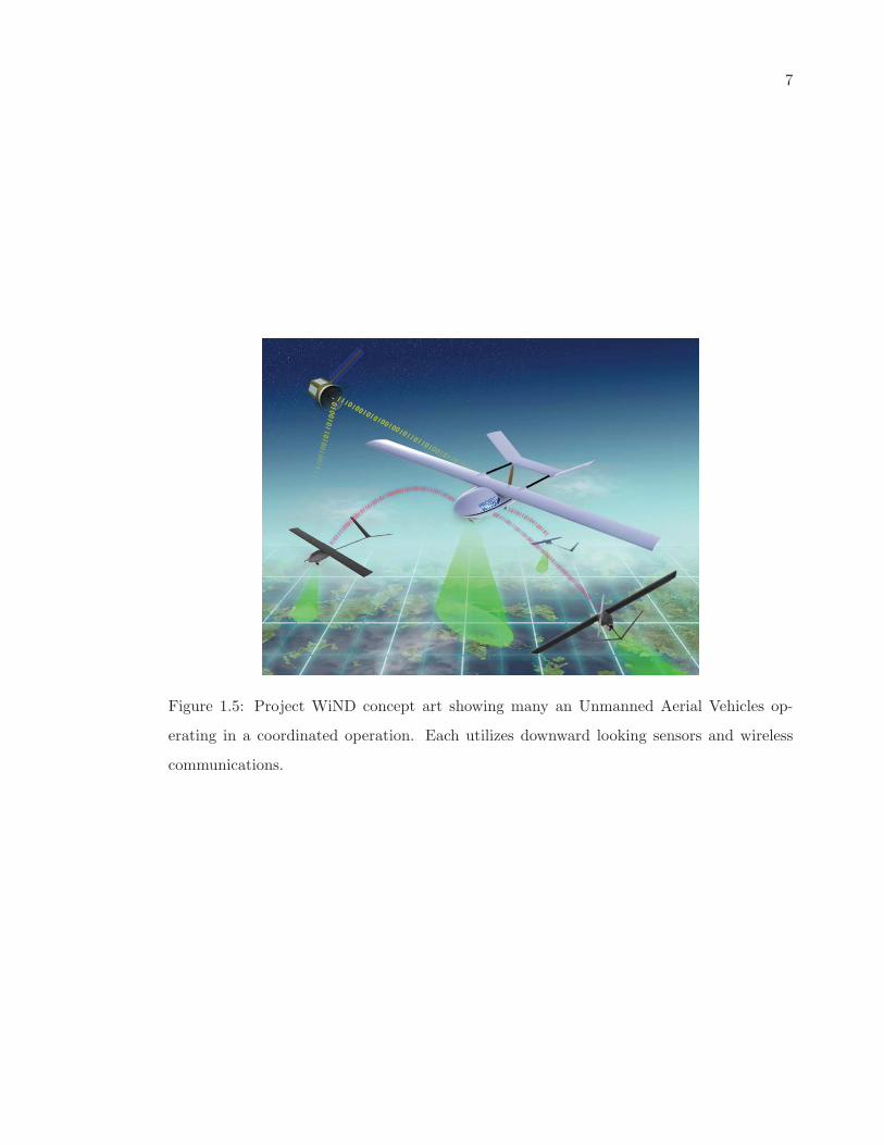
In any system such as this, there will be bottlenecks, whether it be the communications
system or the amount of data presented to human operators at the base station. Too much
data at either bottleneck presents problems. As such, partially distributed processing will
aim to reduce the amount of unneeded data at various bottleneck points.
Figure 1.6: WiND framework architecture showing connection between image processing
module, high level processor, and other communications and flight components.
In most other scenarios, drones in this context are largely ”dumb” in the sense that they
operate by complete remote control, in some cases with minimal autonomy, and transmit
a raw stream of data back to a processing station. Most of the data processing is done
off of the drone itself. In scenarios such as this, the drones may be arguably cheap and
expendable, but this presents overhead on the communications link, and potential overhead
on the data that is presented to human operators.
Full autonomy, in contrast, is costly, difficult, and potentially dangerous, as it puts final
decision making capability in the autonomous system. This comes with a cost overhead as
well, as computing power must be put on the vehicle to allow such autonomy, or a low-
latency data link must be sustained to maintain control by some form of remote automation
system.
In the case of this approach, the project will attempt to provide a platform for apply-
9
ing a better balance of autonomy and remote control. This module will allow drones to
have necessary low-level on-board processing and navigation capability, such that a node
can make decisions on the relevance of sensor data prior to transmission over a limited
communications pipe, or have the capability to navigate back in the event that it loses
communications.
Despite providing more remote autonomy, overarching control will still be done from the
base station, but without as much central overhead. By distribution of low-level processing,
this project’s hypothesis is that data overhead can be reduced and potentially more complex
processing methods could be adopted and utilized with greater ease.
Due to the inherent restrictions of fitting complex equipment on an aerial platform, any
decisions on what processing is put onto the remote vehicle versus being done at a more
powerful command station must be carefully weighed. This framework’s processing modules
must be relatively light and have low enough power requirements to be sustainable, yet be
capable of performing the image processing and navigation tasks required.
By adding remote processing power to the remote platforms, some other advantages
become apparent. For a search and rescue task such as this, sensor data transmission need
not be real-time, so long as the location and time data is preserved. To this end, this
project’s approach will be to evaluate and utilize methods of minimizing data reporting
during runtime by using initial processing resources on remote platforms to intelligently
reduce data throughput needs and effort required on the part of human operators.
1.6 Project Organization and Contributions
This project is one of three cooperative groups at WPI working in a unified effort to
produce the flight platforms, software framework, and communications platform needed to
execute the SAR operations described using the combined efforts of all groups involved.
Shown in Figure 1.7 is the team organization within WPI and with the UNH teams.
The Software team, shown at the top of the WPI portion, will be responsible for the
sensor processing and path planning framework development, and as a secondary effort
work with the individual teams to accomplish integration of the respective platforms as
10
Figure 1.7: Three project components are split between three teams at WPI, and two loosely
associated teams at UNH.
they reach completion. Within the software team, tasks were split between development
of path planning and project interface components, image processing, and communication
methods between the various components of the framework.
1.7 Report Organization
Contained in this report is a description, approach taken, and results gained from this
MQP. First, background will be given on the associated topics and relevant similar work
explored in the fields associated with UAV path planning, image processing, and SAR
operations. Next, the high-level approach proposed by this iteration of the project will be
described in depth, followed by a detailed description of the specific planned implementation
in the provided timespan. The results at the completion of this project will then be outlined,
followed by concluding remarks and suggestions to future teams as to work that could be
done to expand or revise this project based on its findings.
11
Chapter 2
Prior Art
Having established a need for improvements in current Search and Rescue (SAR) tools,
it is now necessary to understand the current SAR system and how to improve it with a
Unmanned Aerial Vehicle (UAV) framework. This framework will support path planning,
navigation, image processing, and extendible modules to interface with communications and
other hardware.
This chapter first establishes current search theory and describes some methods for
planning optimal search routes for an autonomous aerial platform. Next, this chapter
outlines current image processing techniques and how to automate visual detection. Finally,
we present recent research related to unmanned aerial vehicles which combine these topics
and frameworks for aerial platforms . From this, we fully establish the need for a new UAV
framework for SAR applications and the requirements of a framework designed specifically
to support the future of SAR.
2.1 Path Planning
2.1.1 Search and Rescue Theory
Modern search theory rose from Allied military research during World War Two aimed
at developing optimal search methods to locate enemy naval vessels, specifically submarines
[14]. Much of this effort can be traced back to the work of one man, a mathematician named
12
Bernard Koopman, who used probability to predict and optimize search results. However,
it was not until 1973 that Koopman’s research was applied directly to land based search
and rescue operations by Dennis Kelly [9]. Since then, the field of search theory has grown
and is widely adopted today by the like of the United States Coast Guard.
In essence, search theory is about maximizing the probability of success (POS) while
minimizing the effort exerted in a search task. It uses probability and information theory to
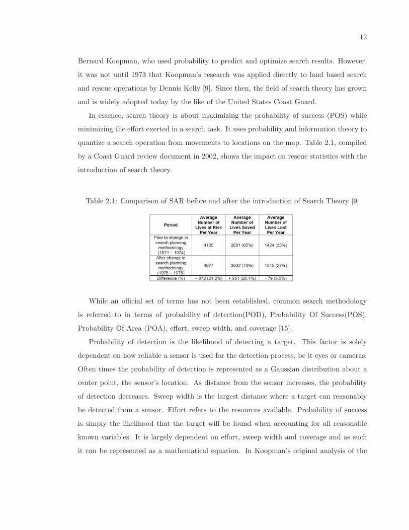
quantize a search operation from movements to locations on the map. Table 2.1, compiled
by a Coast Guard review document in 2002, shows the impact on rescue statistics with the
introduction of search theory.
Table 2.1: Comparison of SAR before and after the introduction of Search Theory [9]
While an official set of terms has not been established, common search methodology
is referred to in terms of probability of detection(POD), Probability Of Success(POS),
Probability Of Area (POA), effort, sweep width, and coverage [15].
Probability of detection is the likelihood of detecting a target. This factor is solely
dependent on how reliable a sensor is used for the detection process, be it eyes or cameras.
Often times the probability of detection is represented as a Gaussian distribution about a
center point, the sensor’s location. As distance from the sensor increases, the probability
of detection decreases. Sweep width is the largest distance where a target can reasonably
be detected from a sensor. Effort refers to the resources available. Probability of success
is simply the likelihood that the target will be found when accounting for all reasonable
known variables. It is largely dependent on effort, sweep width and coverage and as such
it can be represented as a mathematical equation. In Koopman’s original analysis of the
13
random search case, he found this to be equal to,
POS = 1− e−(WL/A)
where ”W” is the sweep width, ”L” the total length of the random search path, and ”A”
the total area to be searched [15].
Now that the key search theory concepts are defined and quantified, we now must
automate the task. To do this, we first solidify the concepts related to artificial intelligence
and path planning.
2.1.2 AI Path Generation
In the field of computer science and the study of Artificial Intelligence (AI) concepts,
path planning is typically just an specific application of a graph search algorithm. Path
planning algorithms range in complexity from single-agent path planning tasks to multi-
agent coordination, and for each of these approaches, the implementation may range from
planning a single step ahead to planning out a full and complex movement plan for a
navigation task. This section will address how these approaches relate and can build off
one another from simplest to most complex.
Figure 2.1: Illustration of a path finding algorithm based on difficulty to traverse (cost).
The numbers in each grid-square denote difficulty and a path is decided by minimizing the
sum of the difficulties in a given path [4].
14
Greedy Algorithms and Single-Agent Heuristics
In computationally constrained scenarios, particularly in embedded processing applica-
tions, fast-running algorithms may at times take precedent over the absolute optimization
of the resulting solution. Furthermore, in some path planning problems, optimal path gen-
eration can become an infeasibly complicated computational task. In such examples, the
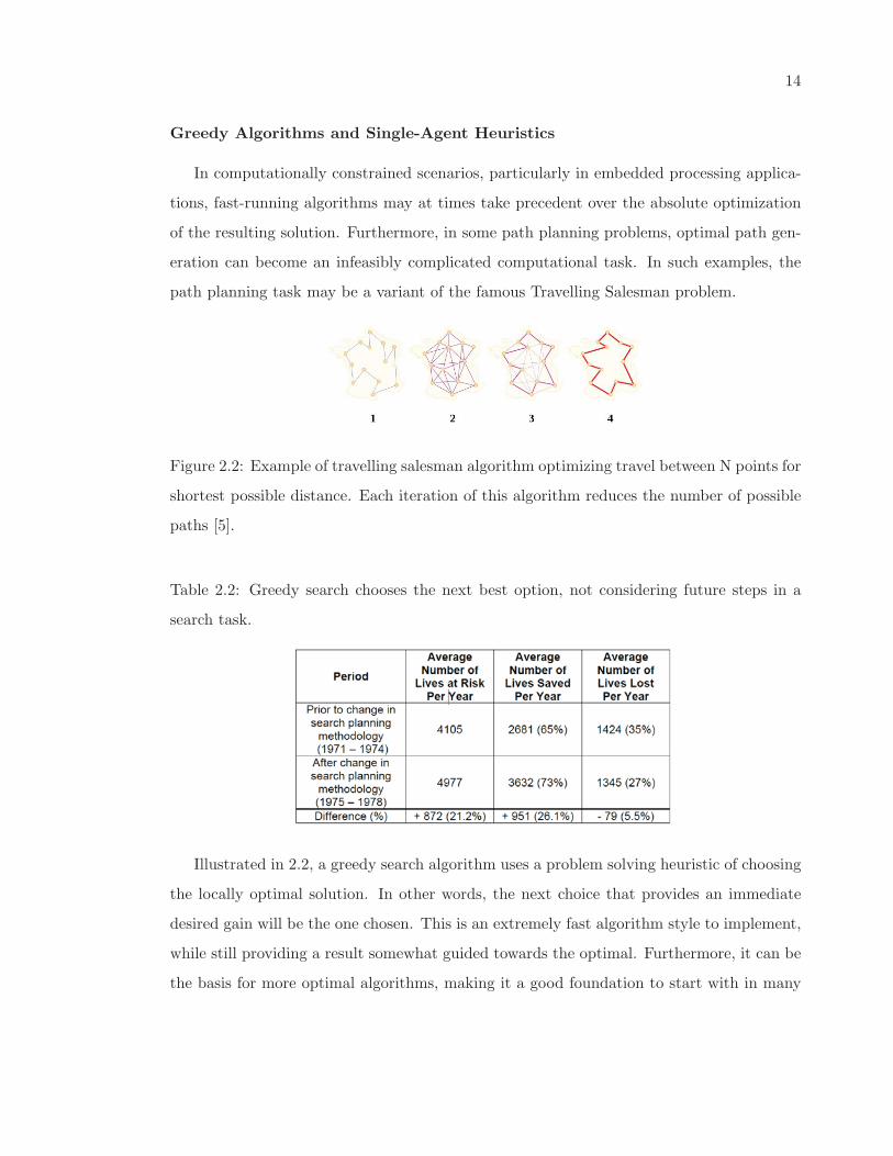
path planning task may be a variant of the famous Travelling Salesman problem.
Figure 2.2: Example of travelling salesman algorithm optimizing travel between N points for
shortest possible distance. Each iteration of this algorithm reduces the number of possible
paths [5].
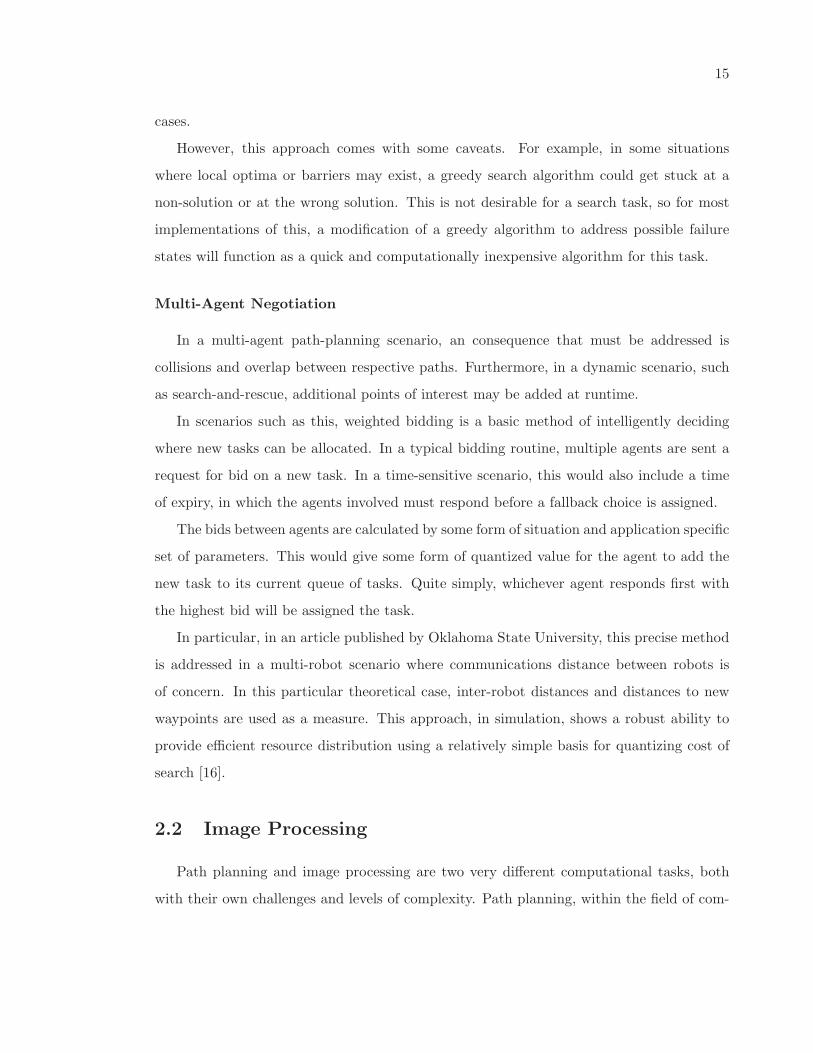
Table 2.2: Greedy search chooses the next best option, not considering future steps in a
search task.
Illustrated in 2.2, a greedy search algorithm uses a problem solving heuristic of choosing
the locally optimal solution. In other words, the next choice that provides an immediate
desired gain will be the one chosen. This is an extremely fast algorithm style to implement,
while still providing a result somewhat guided towards the optimal. Furthermore, it can be
the basis for more optimal algorithms, making it a good foundation to start with in many
15
cases.
However, this approach comes with some caveats. For example, in some situations
where local optima or barriers may exist, a greedy search algorithm could get stuck at a
non-solution or at the wrong solution. This is not desirable for a search task, so for most
implementations of this, a modification of a greedy algorithm to address possible failure
states will function as a quick and computationally inexpensive algorithm for this task.
Multi-Agent Negotiation
In a multi-agent path-planning scenario, an consequence that must be addressed is
collisions and overlap between respective paths. Furthermore, in a dynamic scenario, such
as search-and-rescue, additional points of interest may be added at runtime.
In scenarios such as this, weighted bidding is a basic method of intelligently deciding
where new tasks can be allocated. In a typical bidding routine, multiple agents are sent a
request for bid on a new task. In a time-sensitive scenario, this would also include a time
of expiry, in which the agents involved must respond before a fallback choice is assigned.
The bids between agents are calculated by some form of situation and application specific
set of parameters. This would give some form of quantized value for the agent to add the
new task to its current queue of tasks. Quite simply, whichever agent responds first with
the highest bid will be assigned the task.
In particular, in an article published by Oklahoma State University, this precise method
is addressed in a multi-robot scenario where communications distance between robots is
of concern. In this particular theoretical case, inter-robot distances and distances to new
waypoints are used as a measure. This approach, in simulation, shows a robust ability to
provide efficient resource distribution using a relatively simple basis for quantizing cost of
search [16].
2.2 Image Processing
Path planning and image processing are two very different computational tasks, both
with their own challenges and levels of complexity. Path planning, within the field of com-
16
puter science, is computational problem with solutions that range from trivial to immensely
expensive to compute. Image processing, similarly, addresses many potential computational
problems, with algorithms that may be trivial in concept, but highly difficult to implement
on typical computing hardware. As such, this section will address the relevant background
theory of this field.
Image processing is the practice of using signal processing techniques to take an image as
an input and produce data pertaining to characteristics of interest in the image. Using such
techniques, both hardware and software methods can be implemented to extract important
data from visual input [6, 17].
Many techniques exist for implementing image processing. Image processing can be
implemented in pure software, often with the aid of a code library such as OpenCV [18].
However, given the nature of image processing, some implementations in pure code are
far from optimal.[6] Since an image is represented as a 2-dimensional matrix of pixels,
traditional serial processing methods may handle an image one pixel at a time. If quick
processing of video data is desired, this may be too inefficient for the convenience of pure
code. For example, operating on a standard 640 by 480 pixel image at 15 frames per second
requires processing 4.6 million pixels per second. At multiple operations per pixel, this
rapidly becomes quite a computationally expensive task.
Newer technologies, such as Graphics Processing Units (GPUs) and Field Programmable
Gate Arrays (FPGAs), are designed specifically for processing tasks of this type, rather than
generalized processing tasks that CPUs are built to handle. This is often at the cost of some
coding conveniences, but allows image processing tasks to be executed in a tremendously
more efficient manner. [17] With proper implementation on such hardware, image processing
algorithms can be executed on every pixel of an image simultaneously. On FPGAs, this
specialization goes one step further, as the digital logic behind the image processing can be
implemented in hardware itself.
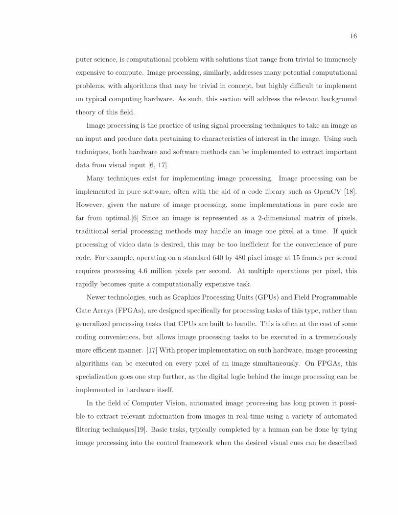
In the field of Computer Vision, automated image processing has long proven it possi-
ble to extract relevant information from images in real-time using a variety of automated
filtering techniques[19]. Basic tasks, typically completed by a human can be done by tying
image processing into the control framework when the desired visual cues can be described
17
(a) Original Image: Various coins on a surface with
varying orientations and arrangement
(b) Processed Image: Individual coins are discerned
from the background texture, highlighted, and num-
bered based on location of center point
Figure 2.3: Example of a blob detection algorithm running in MATLAB
in code [20].
Prior Technique
There are many publications on systems which combine image processing and computer
vision with unmanned areal vehicles for feature detection and navigation[21, 22, 23, 24].
However, there is less research focused on developing for systems based on low-power pro-
cessors such as our target platform [25, 26].
Past projects have taken a hardware approach to image processing using FPGAs to
accelerate high-complexity algorithms [27]. Research at Brigham Young University achived
a fully on-board stabilization system for a small quad-rotor platform by using parallelized
algorithms on an FPGA. To achieve stabilization, they hardware-implemented complex
algorithms such as template matching, feature correlation, and distortion correction.
Other research has combined hardware and software for accelerated image processing
[28, 29]. In these applications, the combined power of a DSP and FPGA together perform
18
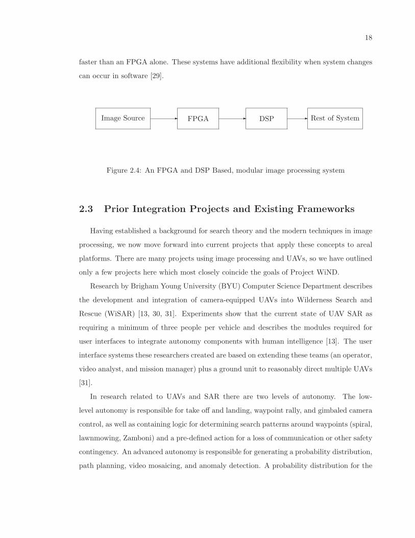
faster than an FPGA alone. These systems have additional flexibility when system changes
can occur in software [29].
Image Source FPGA DSP Rest of System� � �
Figure 2.4: An FPGA and DSP Based, modular image processing system
2.3 Prior Integration Projects and Existing Frameworks
Having established a background for search theory and the modern techniques in image
processing, we now move forward into current projects that apply these concepts to areal
platforms. There are many projects using image processing and UAVs, so we have outlined
only a few projects here which most closely coincide the goals of Project WiND.
Research by Brigham Young University (BYU) Computer Science Department describes
the development and integration of camera-equipped UAVs into Wilderness Search and
Rescue (WiSAR) [13, 30, 31]. Experiments show that the current state of UAV SAR as
requiring a minimum of three people per vehicle and describes the modules required for
user interfaces to integrate autonomy components with human intelligence [13]. The user
interface systems these researchers created are based on extending these teams (an operator,
video analyst, and mission manager) plus a ground unit to reasonably direct multiple UAVs
[31].
In research related to UAVs and SAR there are two levels of autonomy. The low-
level autonomy is responsible for take off and landing, waypoint rally, and gimbaled camera
control, as well as containing logic for determining search patterns around waypoints (spiral,
lawnmowing, Zamboni) and a pre-defined action for a loss of communication or other safety
contingency. An advanced autonomy is responsible for generating a probability distribution,
path planning, video mosaicing, and anomaly detection. A probability distribution for the
19
search area is created by a Bayesian model incorporating human behavior and terrain, as
well as a Markov chain Monte Carlo Metropolis-Hasting algorithm to generate distribution
changes over time. Path planning is handled by a combination of the Generalized Contour
Search and the Intelligent Path Planning algorithms published in the IEEE International
Workshop on Safety, Security, and Rescue Robotics and the Journal of Field Robotics
respectively [13].
Using quad-rotor style UAVs with downward facing cameras, the researchers at the
University of Oxford Computing Library developed navigation algorithms for use with SAR.
The algorithms were all based on probabilistic maps and developed to ”cope with the
uncertainties of real-world deployment.” The team used Greedy Heuristics, Potential-based
Heuristics, and Partially Observable Markov Decision Process (POMDP) based heuristics.
Greedy Heuristics are strategies based on navigating adjacent cells on a probabilistic map,
a more advanced variant of this ”1-look ahead” was also used. Potential-based Algorithms
model goals and obstacles with association and repulsion potentials. POMDP algorithms
are a generalization of a Markov Decision Process which optimizes reward against cost of
potential actions [32].
The Cooperative Control for UAV Teams project from Massachusetts Institute of Tech-
nology Aerospace Controls Laboratory used multiple fix-winged aircraft with GPS feeds
combined with a centralized AI to deduce feasible paths around obstacles in the environ-
ment while maintaining a path to an objective. The approach uses an extended pedal
method named Receding Horizon Task Assignment (RHTA) for real time task assignment
and reassignment. Trajectory Optimization is solved using a MILP-based receeding horizon
planner RH-MILP. This algorithm gives a ”cost-to-go” estimate of each path [33].
In regards to human-UAV interaction, the Phairwell system, developed by BYU, is
an augmented virtual reality interface where the operator assigns each UAV in a group a
specific task based on input from the video analyst and manager. The Wonder Client for
Video Analyst allows the analyst to choose between live video and mosaic views. The video
analyst then annotates the video with candidate objectives, these tags are automatically
geo-referenced and shown on future video streams. The wonder Client for Mission manager
provides the manager with high-level information on what has been searched and how well.
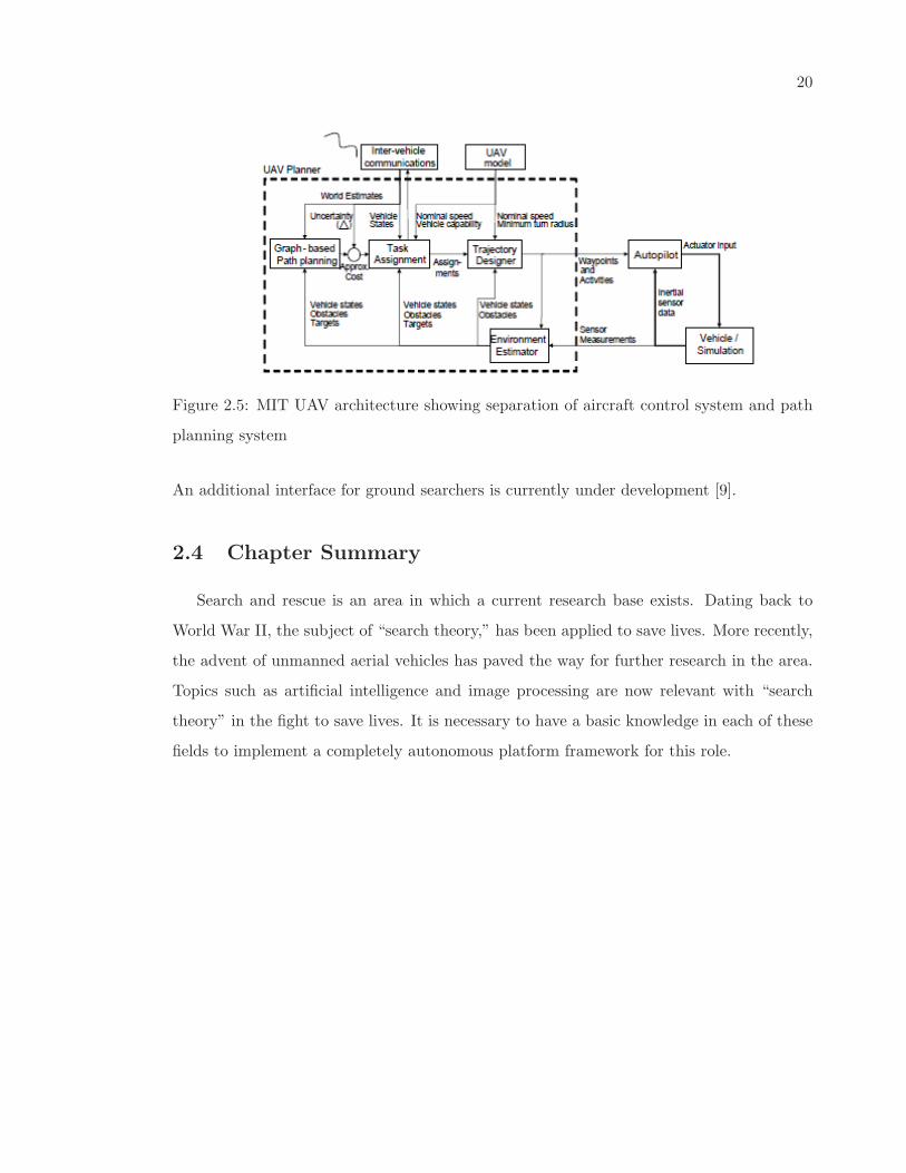
20
Figure 2.5: MIT UAV architecture showing separation of aircraft control system and path
planning system
An additional interface for ground searchers is currently under development [9].
2.4 Chapter Summary
Search and rescue is an area in which a current research base exists. Dating back to
World War II, the subject of “search theory,” has been applied to save lives. More recently,
the advent of unmanned aerial vehicles has paved the way for further research in the area.
Topics such as artificial intelligence and image processing are now relevant with “search
theory” in the fight to save lives. It is necessary to have a basic knowledge in each of these
fields to implement a completely autonomous platform framework for this role.
21
Chapter 3
Proposed Approach
By adding a level of intelligence above otherwise blind sensor-polling and manual path
planning tasks, this system will provide an accessible means of managing and allocating
important resources in search and rescue operations, both in personnel and data overhead.
The planned architecture will emphasize modularity and portability, especially between its
own individual components. This involves the creation of two modules: a path planning
module, and an image processing module. Within the UAV fleet, the these modules should
be capable of integrating with both the central ground station and the individual drones to
simplify high-level management of the existing autopilot and other sensor hardware.
For example, the path planning components would provide a means of generating the
waypoints needed for a UAV to search a given area, rather than requiring the end user to
manually enter a flight plan. For sensor data, this would also need to be able to provide
a high degree of control over data reporting capabilities; that is, what sensor data is sent
where in the system, and in what format. In the case of image processing, in a search an
rescue operation, this system should assist in the detection of persons on the ground from
the UAV, rather than blindly streaming all camera data. Instead, it should provide some
informative data on the images and control over what image data is sent back or logged.
Overall, this system should facilitate resource management, whether it be effort needed
from the persons involved, or reduce unneeded use of limited storage or bandwidth.
As such, the ultimate goal will be a framework that can be used to accomplish these
22
path-planning and image processing tasks, while providing end users and developers the
flexibility to expand on and reconfigure the existing system.
3.1 Framework Architecture
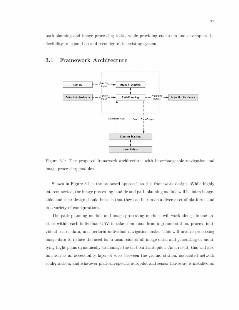
Figure 3.1: The proposed framework architecture, with interchangeable navigation and
image processing modules.
Shown in Figure 3.1 is the proposed approach to this framework design. While highly
interconnected, the image processing module and path planning module will be interchange-
able, and their design should be such that they can be run on a diverse set of platforms and
in a variety of configurations.
The path planning module and image processing modules will work alongside one an-
other within each individual UAV to take commands from a ground station, process indi-
vidual sensor data, and perform individual navigation tasks. This will involve processing
image data to reduce the need for transmission of all image data, and generating or modi-
fying flight plans dynamically to manage the on-board autopilot. As a result, this will also
function as an accessibility layer of sorts between the ground station, associated network
configuration, and whatever platform-specific autopilot and sensor hardware is installed on
23
each UAV, allowing uniform access, coordination, and management of UAVs even in the
presence of differing platform capabilities.
3.2 Path Planning
For a UAV to function autonomously, it needs some method for flying without full
direction from a human operator. With an autopilot, this may involve automated flight
stabilization, and execution of pre-defined flight routines. Flight plans, however, still may
require human intervention to generate, verify, and coordinate between multiple UAVs. A
path planning component, in this case, would provide a means of generating flight plans
based on higher level requirements given by a human operator, saving them the time and
effort they otherwise may spend doing this manually.
For the navigation component, the planned approach is to implement two to three basic
algorithms on a platform capable of handling individual path planning tasks, negotiation,
and resource allocation between multiple platforms. Since countless algorithms exist for
completing these tasks, some of which were outlined previously, it is in the best interests
for the scope of this project to lay a basic, functional foundation for this component. This
can serve as a proof of concept and easily be expanded on as needed. As such, usability
and expandability are major design considerations over depth and sophistication.
As development of an autopilot is a lengthy and highly platform specific task, the navi-
gation module does not operate as an autopilot, nor was it decided to be part of the project
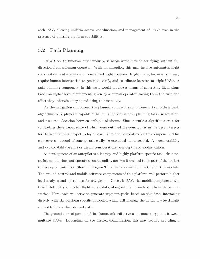
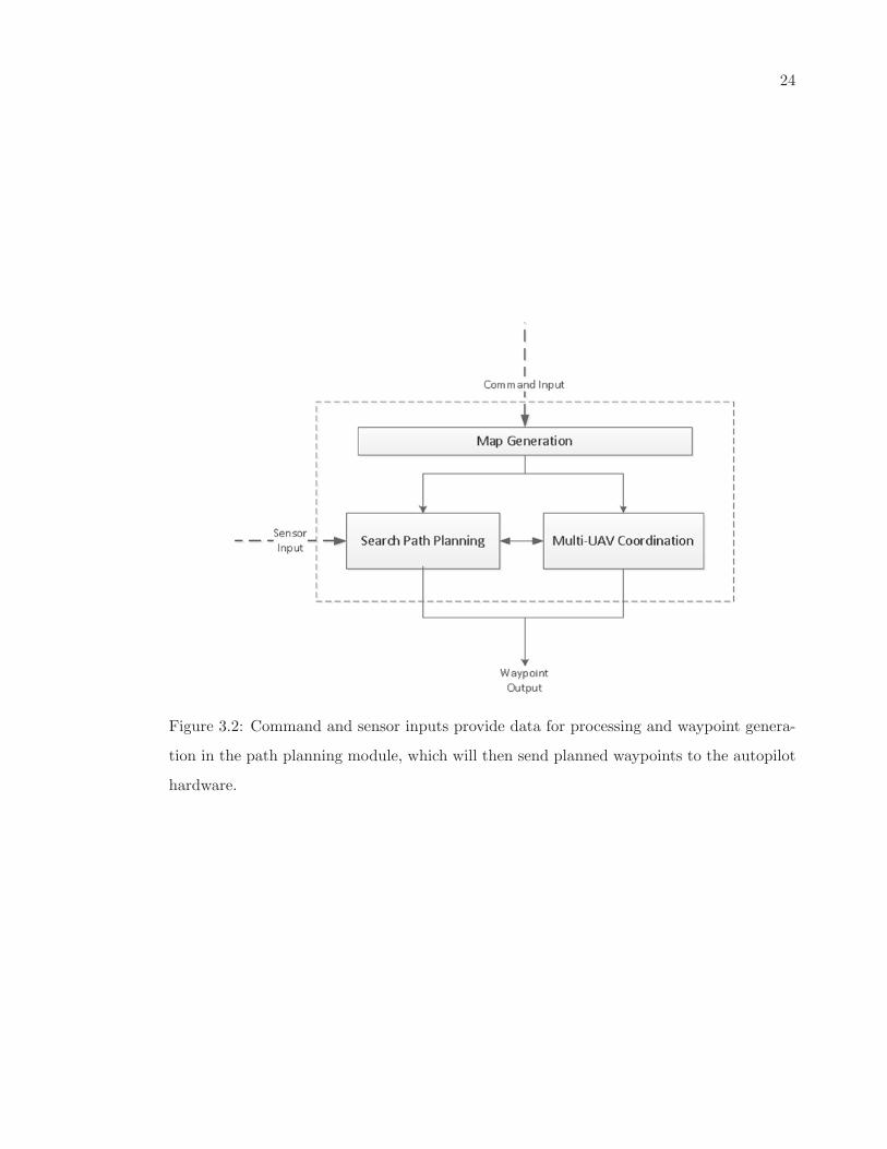
to develop an autopilot. Shown in Figure 3.2 is the proposed architecture for this module.
The ground control and mobile software components of this platform will perform higher
level analysis and operations for navigation. On each UAV, the mobile components will
take in telemetry and other flight sensor data, along with commands sent from the ground
station. Here, each will serve to generate waypoint paths based on this data, interfacing
directly with the platform-specific autopilot, which will manage the actual low-level flight
control to follow this planned path.
The ground control portion of this framework will serve as a connecting point between
multiple UAVs. Depending on the desired configuration, this may require providing a
24
Figure 3.2: Command and sensor inputs provide data for processing and waypoint genera-
tion in the path planning module, which will then send planned waypoints to the autopilot
hardware.
25
simple linking point from the system to a user interface for data display and command
input, or further processing of accumulated data from all the UAVs in the network. As
individual UAV functionality is a stepping stone that must be addressed before multi-UAV
coordination can be fully tested, this will first take the form of a simple central interface.
For the autopilot, the hardware team chose a pre-made platform, the Paparazzi, as it
is an open-source and relatively well established autopilot platform [34]. It uses the Ivy
software bus, a network communications library developed by ENAC research in France, to
handle message routing between a ground control software platform and the firmware on
the actual mobile autopilot module [35]. From there, it can execute basic flight commands
at three levels of autonomy: simple passthrough flight control, stabilized remote controlled
flight, and full autonomous flight. The path planning component, in contrast, will link the
individual flight module with the overarching framework.
Since this module is capable of taking in flight plans in the form of waypoint lists, execute
pre-configured flight routines on command (such as a surveying routine for a given area),
and update waypoints at runtime, it will be used to handle the backend navigation tasks.
The software module’s navigation and path planning task will thus be to generate waypoints
and routine commands to then delegate to the autopilot module itself. This way, our module
can function to overlay more sophisticated and automated path-generation methods on the
pre-existing abilities of the autopilot, and ease the interface between multiple such platforms
and the ground station using them.
By providing an accessible and portable module for these path planning tasks, this com-
ponent will provide an enhancement over the existing usability and resource management
capabilities of such autopilot software. The Paparazzi autopilot, like many other hobby
oriented options, requires a full ground control suite to be installed for normal use, and
customization requires modification of much of the platform-specific code for the autopilot.
Furthermore, it does not provide the types of high-level management functions proposed,
but rather basic manual path planning, and tuning utilities for the specific autopilot.
In contrast, the proposed path planning module would address this by providing an
overarching layer for managing high-level tasks, into which a wide variety of autopilot
modules to be interfaced in a uniform manner to a single reconfigurable system. This would
26
allow users of a variety of platforms to benefit from reduced command and coordination
efforts in a search and rescue task, without the development overhead or architecture rigidity
of modifying a specific platform’s autopilot.
3.3 Image Processing
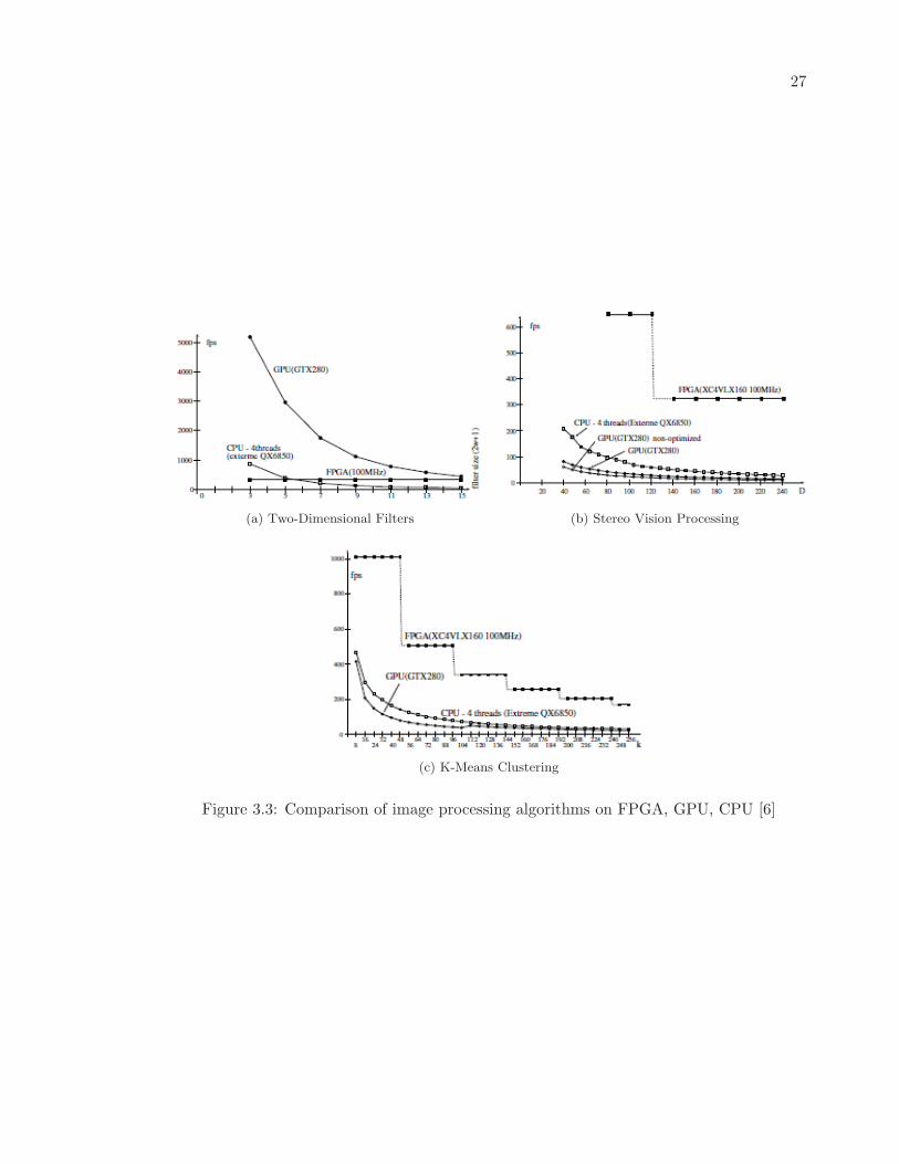
The proposed image processing component is broken down across two subsystems, a
Field Programmable Gate Array (FPGA) co-processor with on-die Digital Signal Proces-
sors (DSP), and the software platform, an ARM CPU with on board graphics processing
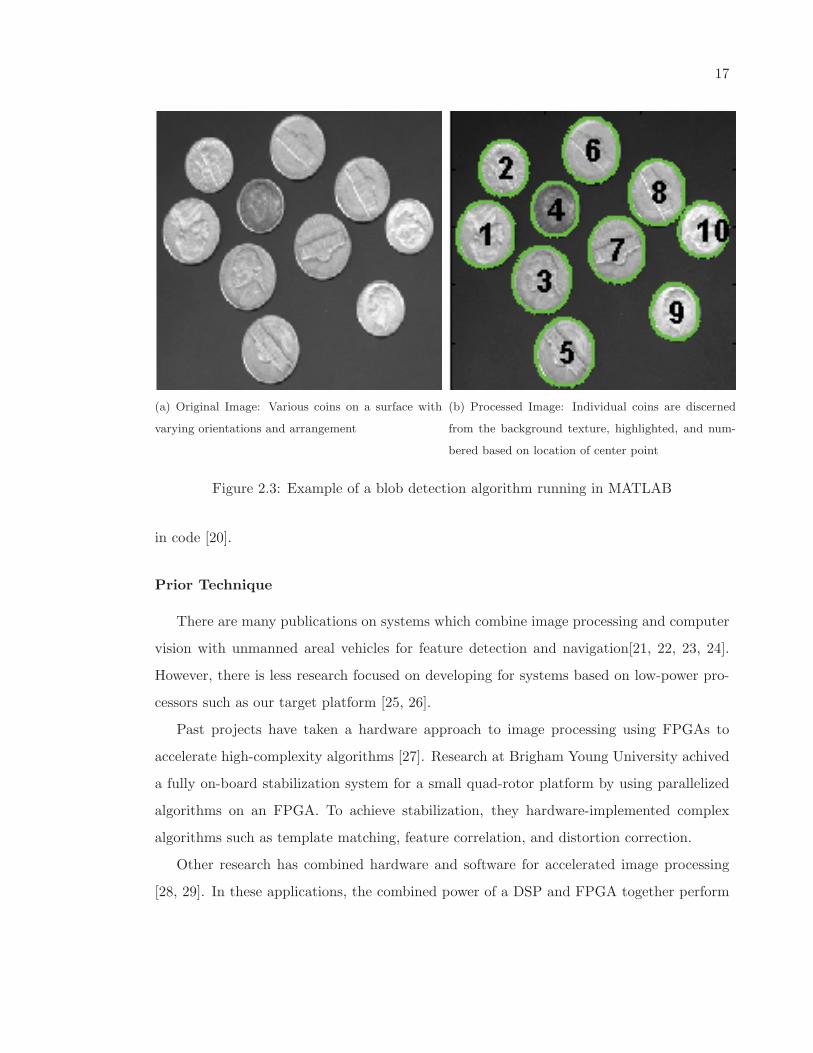
unit (GPU). The choice of using four different types of data processing devices- DSP, FPGA,
CPU, GPU - comes from comparisons of different algorithms on different platforms con-
ducted at the University of Tsukuba. The comparison shows that no data processing device
has a clear advantage in real time image processing. In the test of two-dimensional filters,
the GPU had a much higher throughput for filters using small numbers of pixels but per-
formance decayed rapidly with increasing swatch size [6]. The results also show that the
FPGA has higher theoretical throughput in stereo-vision processing and an implementation
of the k-means clustering algorithm, however the development overhead to create FPGA
modules is much higher than for software, and for these algorithms the CPU had better
performance than the GPU [6]. While these comparisons were not performed with the exact
hardware or algorithms we used, it was decided that the mixed results showed a need for
different implementation options.
3.3.1 FPGA-DSP
FPGAs are advantageous in highly parallelized, high-bandwidth operations [6]. In some
situations, the entire image processing subsystem may reside in hardware and the CPU-GPU
system may be entirely dedicated to AI and path planning. Current FPGA manufactures
such as Xilinx now include ”DSP Slices” to improve FPGA utilization and allow for higher
operating frequencies [36].
Our implementation includes on-chip buffers and memory for frame-wise operations
such as filtering and multi-frame operations such as motion capture. The communication
27
(a) Two-Dimensional Filters (b) Stereo Vision Processing
(c) K-Means Clustering
Figure 3.3: Comparison of image processing algorithms on FPGA, GPU, CPU [6]
28
between the CPU-GPU is flexible and can operate at speeds up to 12Mbps.
Unfortunately, the development overhead of describing many image processing algo-
rithms in HDL is much higher than for software. This is partially due to limitations in
the current languages and partially due to the proliferation of image processing libraries
available for software platforms such as OpenCV and the Matlab Image Processing Toolbox.
3.3.2 CPU-GPU
As part of our focus on developing a flexible and scalable framework for SAR UAVs,
we did not limit the developer’s ability to process sensor input in hardware or software.
The developer can choose not to utilize the FPGA-DSP at all or, more realistically, to to
implement part of the image processing subsystem on the FPGA-DSP and the rest in GPU
accelerated software. This allows pre-processing or filtering to take place on a platform more
suited for the task, and then the highly complex, more sequential mathematical operations
to occur in the more flexible environment. This should enable developers to obtain real
time performance without sacrificing flexibility.
The example algorithm we developed for this project calculates statistical perimeters
on the FPGA-DSP and filters incoming frames to binary images. The CPU-GPU, utilizing
the libraries available in OpenCV, would then perform a blob detection and tracks these
blobs across multiple frames, eventually deciding if the current location contains a possible
person of interest.
3.4 Framework Considerations
In order to make this system appropriately flexible and portable, the approach involved
designing the broad foundation of the framework itself, with each module containing enough
baseline implemented functionality to show that the overall concept of the system works.
That is, the ability of the image processing module and path planning module to perform
a demo of their desired tasks.
Furthermore, as a framework, it was important to design the code base in a portable
manner. As such, it is expected that the framework will consist of one or more libraries that
29
can be installed on the platform operating system. This will allow other code to access the
library, without the need to recompile the library every time something changes in a project
implementing it, or conversely recompiling every project using it when backend library code
is changed.
Given the breadth of this task, design choices had to be made to further reflect the time
and resource restraints associated with this project. To avoid ”feature creep” preventing
useful progress, not all components are expected to be utilized to their fullest depth in a
single iteration of the project, but necessary functionality will be identified, researched, and
groundwork laid to provide the means of implementing the breadth of features desired.
3.5 Chapter Summary
Proposed here is a design for a framework that performs path planning and image
processing tasks in a UAV network for search and rescue applications. The path planning
component will provide enhancement over the default portability, flexibility, and effort
required to use existing autopilot modules, while reducing the effort needed on the part of
the operator. The image processing module will provide further enhancement over blindly
reporting sensor data, granting the ability to apply some initial processing of image data
in its pure, uncompressed form and intelligently report metrics on this data, even in the
absence of bandwidth normally needed to stream video.
Overall, this system will provide a layer of enhancement over the integration of existing
autopilot and image capture modules, letting developers more easily configure the system
to a desired architecture and compensate for bottlenecks in data throughput that might
otherwise render some systems unusable. More importantly, for the end user, this will
allow UAV based search and rescue missions to be deployed with less resources spent in the
planning and coordination of the aircraft involved.
30
Chapter 4
Implementation
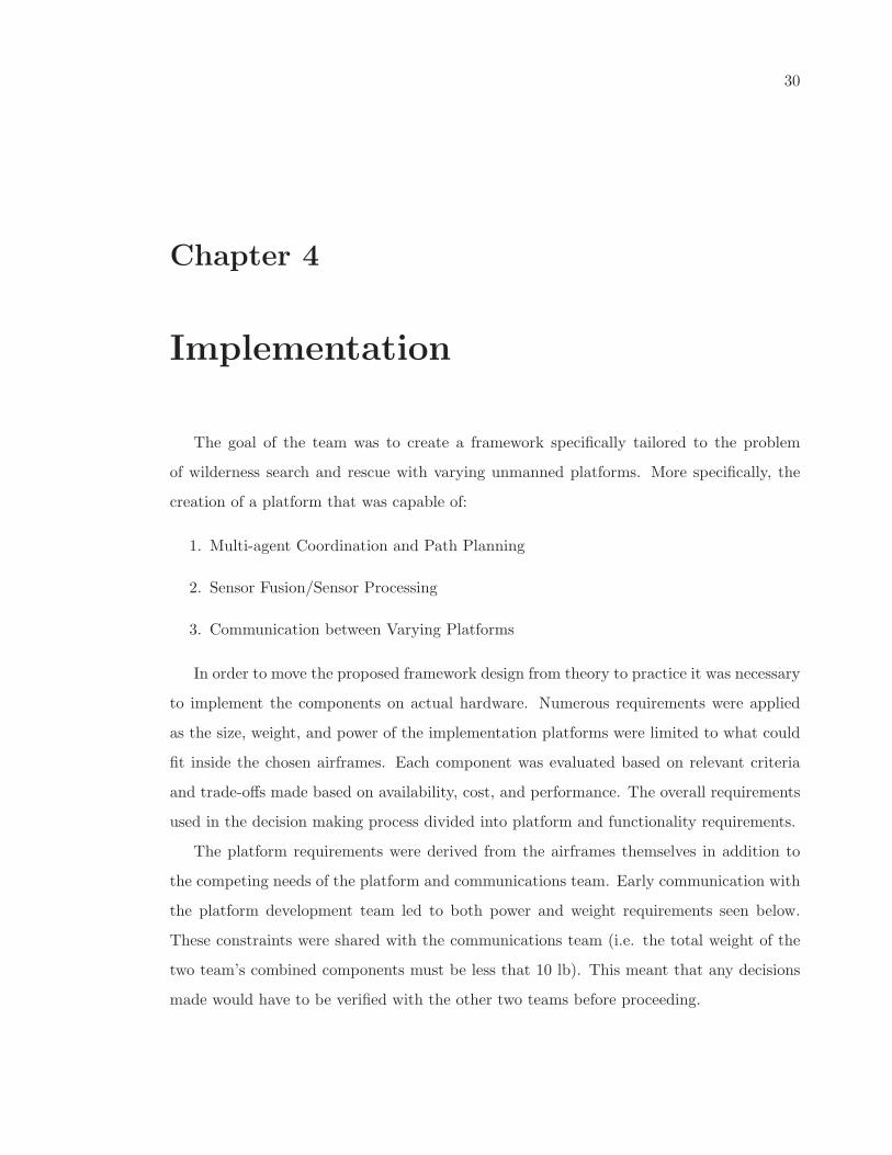
The goal of the team was to create a framework specifically tailored to the problem
of wilderness search and rescue with varying unmanned platforms. More specifically, the
creation of a platform that was capable of:
1. Multi-agent Coordination and Path Planning
2. Sensor Fusion/Sensor Processing
3. Communication between Varying Platforms
In order to move the proposed framework design from theory to practice it was necessary
to implement the components on actual hardware. Numerous requirements were applied
as the size, weight, and power of the implementation platforms were limited to what could
fit inside the chosen airframes. Each component was evaluated based on relevant criteria
and trade-offs made based on availability, cost, and performance. The overall requirements
used in the decision making process divided into platform and functionality requirements.
The platform requirements were derived from the airframes themselves in addition to
the competing needs of the platform and communications team. Early communication with
the platform development team led to both power and weight requirements seen below.
These constraints were shared with the communications team (i.e. the total weight of the
two team’s combined components must be less that 10 lb). This meant that any decisions
made would have to be verified with the other two teams before proceeding.
31
1. The total combined weight must be under 10 lb.
2. All components must be able to fit within the chosen airframe
3. The total power draw from all components must be under 120W
The functionality requirements of the component choice were drawn from the project
goal, the creation of a SAR framework.
4.1 System Architecture
To meet these design goals, the framework design proposed earlier must be solidified
into specific hardware components, functionalities, and requirements.
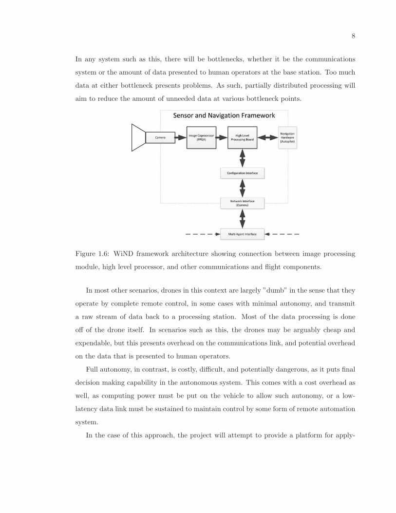
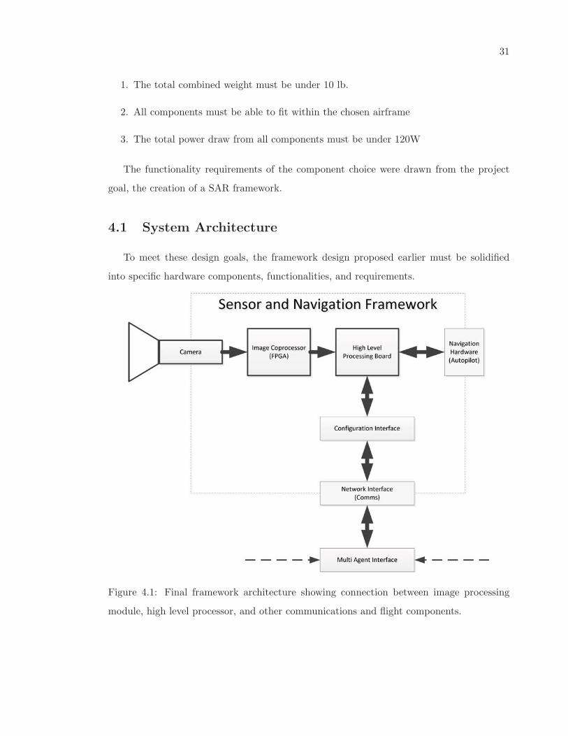
Figure 4.1: Final framework architecture showing connection between image processing
module, high level processor, and other communications and flight components.

32
Shown in Figure 4.1 is the final proposed system architecture. The image processing
will primarily be targeted at a discrete coprocessor board, connected directly to the camera
and the high level processing board, which will direct path planning, data routing, and
general framework configuration tasks. These will link with the communications team’s
platform for network connectivity, and the hardware team’s autopilot and flight sensors for
data collection and waypoint control of the individual UAVs.
This will also connect to a ground-station component, which will allow data visualization
of messages sent from the UAVs, and command input to the framework itself.
4.2 Navigation Module Development
The hardware needed to have sufficient processing power to run a basic Linux operating
system. In doing so, this would remove much of the hardware-specific coding that would
need to be done to deal with networking and data acquisition tasks. At the same time,
initial hardware considerations included the capability to perform basic image processing
tasks, such as video compression or filtering, and be capable of interfacing with the autopilot
module that the hardware team would choose for the flight platform.
Early research was weighted between various small form-factor Intel Atom boards, ARM
processor boards, and FPGA development boards. Initially this led to choices of develop-
ment boards with both an ARM processor and an FPGA on the same module. However,
availability of such hardware led us to split our module into the purchase of two separate
boards. While not necessarily as compact as a single-board option, this allowed for greater
flexibility in what was used for each platform.
4.2.1 Hardware Choice
The high-level processing module was chosen from two main categories: mini/pico-ITX
Intel-based motherboards, and ARM-based development boards. Initial hardware compar-
isons were made with low-voltage Intel Core i5 and i7 model ITX boards, however these
boards were disproportionately expensive and power inefficient (100 watts being the esti-
mated power needed for a low-voltage i7 board at full processor usage). This shifted focus
33
towards Intel Atom based boards and ARM development boards.
As can be seen in Table B.1, in comparison with virtually every Intel based board,
the ARM development boards had substantially less power demand in proportion to the
reported processing power. Atom based systems were typically in the 1 to 1.6 GHz single-
core range, while ARM platforms ranged from 700MHz single-core to 1Ghz dual core. These
platforms were also typically far less expensive than the Intel based platforms.
Another platform considered early on was the Raspberry Pi. This platform was sub-
stantially smaller and less expensive than other ARM platforms in its category, with very
comparable hardware. However, accessibility was an issue when looking into acquiring this
platform, as it was not released at the time of purchasing, and currently is only available
in very limited quantities.
The final choice came down to boards using the TI OMAP ARM processor series. The
most prevalent of these platforms are the OMAP 3000 series platforms, which include the
multiple variants of the Beagleboard (BeagleBoard, BeagleBoard xM, and recently released
BeagleBone). These boards range in processing speed from 700 MHz to 1 GHz on the ARM
Cortex-A8 architecture, and include an onboard media acceleration chip and DSP. Many
projects of similar nature have used this platform.
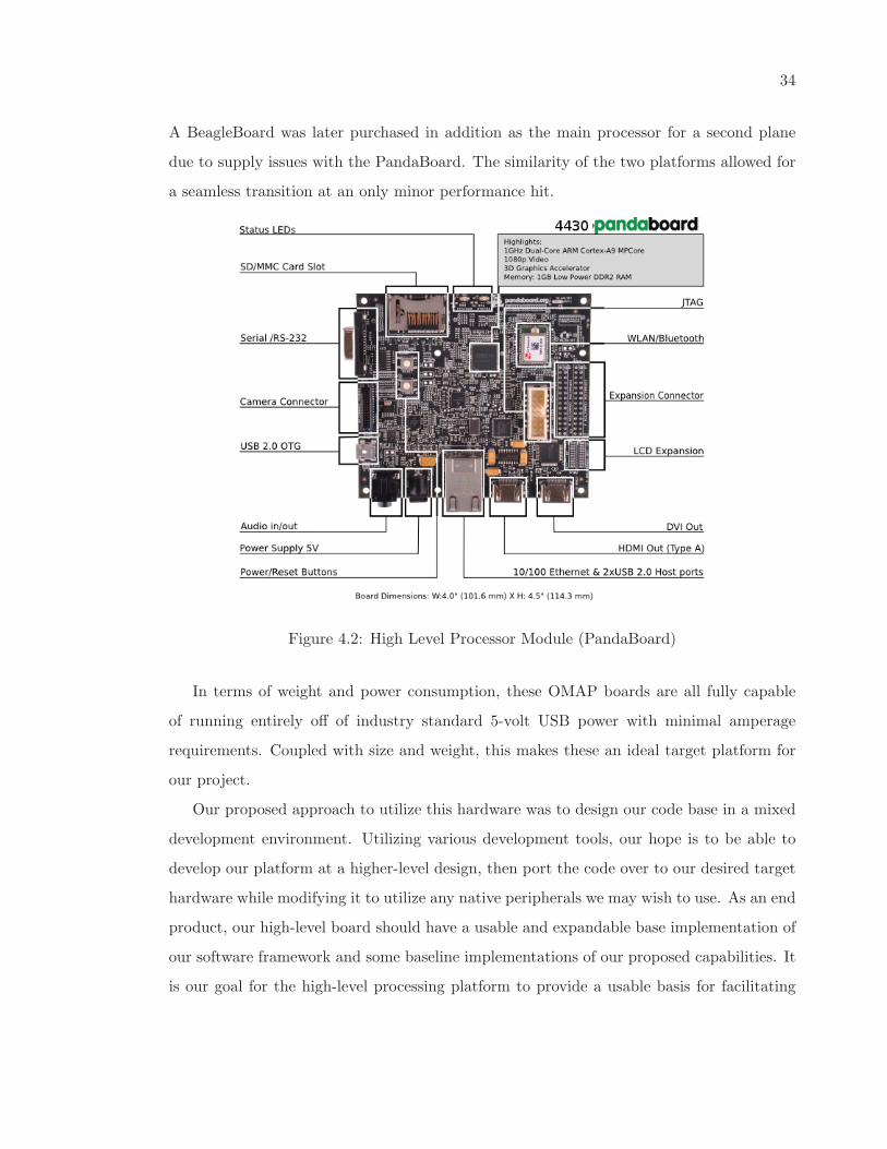
Similar to these platforms is the PandaBoard, which uses the newer OMAP 4430 pro-
cessor, a dual-core 1 GHz ARM Cortex-A9, and is advertised as having enhanced media
acceleration from the BeagleBoard platform.
All of these OMAP platforms are capable of running variants of known Linux distri-
butions. Ubuntu, a Debian-based distribution, and Angstrom, a natively compiled Linux
distribution for embedded devices, are among the most popular operating systems for these
platforms.
The respective similarities between the BeagleBoard variants and the PandaBoard, along
with their price range, led to choosing the PandaBoard as the initial high-level processor
module. The BeagleBoard was more readily available and a more mature product then the
PandaBoard, and has thus been used in many more projects. However, the PandaBoard had
the most capable ARM processor, and boasted enhanced HD-capable media acceleration.
For these reasons, the PandaBoard was chosen as our initial high-level processing platform.
34
A BeagleBoard was later purchased in addition as the main processor for a second plane
due to supply issues with the PandaBoard. The similarity of the two platforms allowed for
a seamless transition at an only minor performance hit.
Figure 4.2: High Level Processor Module (PandaBoard)
In terms of weight and power consumption, these OMAP boards are all fully capable
of running entirely off of industry standard 5-volt USB power with minimal amperage
requirements. Coupled with size and weight, this makes these an ideal target platform for
our project.
Our proposed approach to utilize this hardware was to design our code base in a mixed
development environment. Utilizing various development tools, our hope is to be able to
develop our platform at a higher-level design, then port the code over to our desired target
hardware while modifying it to utilize any native peripherals we may wish to use. As an end
product, our high-level board should have a usable and expandable base implementation of
our software framework and some baseline implementations of our proposed capabilities. It
is our goal for the high-level processing platform to provide a usable basis for facilitating
35
the path-planning and data reporting process of SAR missions.
4.2.2 Path Planning Development
For the path planning module, the map structure needed to be carefully considered be-
fore implementation. To provide this functionality in the framework, a robust but manage-
able map structure needed to be chosen that would provide advantages for both individual
UAV path planning, and coordination of search operations between multiple UAVs.
A simple method to initially implement multi-agent coordination is to use a map struc-
ture that allows well defined allocation of search areas to a single UAV, such that there is no
ambiguity as to which UAV should be in a given area at a given time. Furthermore, com-
pared with a dynamic traffic control approach, this reduces the processing effort necessary
on the system for coordination. As such, the individual UAV path planning tasks could be
focused on primarily, and basic multi-UAV coordination built off of this functionality.
As mapping tasks necessary in a search and rescue mission would largely comprise
tracking sensor data on individual portions of the map, a cell-based map was chosen as it
provides a means of classifying and localising an otherwise continuous collection of data
points. For this purpose, cell geometry is a simple choice between the only three shapes
that uniformly tessellate; triangles, squares, and octagons.
For navigation purposes and programming purposes alike, cell-based grids typically
would use a Cartesian coordinate system (x and y coordinates on perpendicular axes)
and square cell geometry. This choice is logical when considering the intuitive nature of
a Cartesian coordinate system, and the ease by which this data can be represented and
addressed in code as a two dimensional array of values. However, from the standpoint of
path planning, there are a number of disadvantages to a square cell geometry.
From a computing standpoint, a square-grid was more intuitive, and can be represented
in memory more easily. However, in grid-based search algorithms in general, consideration
needs to be made for the conditions by which an agent might cross between cells. Across
edges between known, adjacent cells, this was not an issue, however corner crossings risk
passing into undesired cells. This is especially important in path planning as crossing
between cells should be safe for the craft involved, risk of crossing into unwanted cells
36
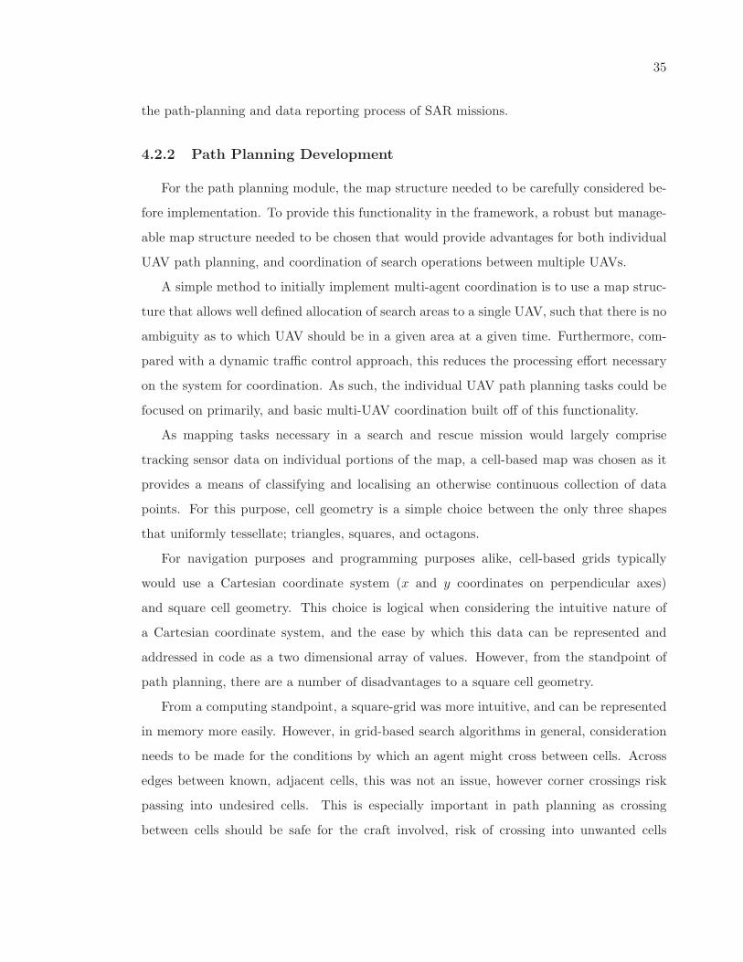
Figure 4.3: Hexagonal cells provide higher edge-crossing options than square grid cells.
should be avoided, thus reducing the options of movement when planning a path. As can
be seen in Figure 4.3, hexagonal cells provide substantial navigational benefit in this respect.
As opposed to four edge crossings and four corner crossings to adjacent cells in a square grid,
the hexagonal geometry provides edge-crossings and no corner crossings on all six adjacent
cells, a 50% improvement in safe cell traversal options with no wasted adjacent space.
Addressing the coordinate system in such a search grid is another problem which had
to be considered if this was to be implemented. Square grids are simple to describe a
coordinate system for, but options for this choice needed to be explored before ruling it out.
The naive approach to solving this problem may involve addressing hexagonal cells in
perpendicular rows and columns, in an attempt to emulate a Cartesian coordinate system.
However, hexagonal cells do not pack in a perpendicular orientation. As such, this method
becomes inefficient as it involves a non-uniform conversion between grid coordinates and
actual global coordinates in Cartesian space. The same formula cannot be used to convert
all coordinates between systems. However, an elegant solution was devised to address this.
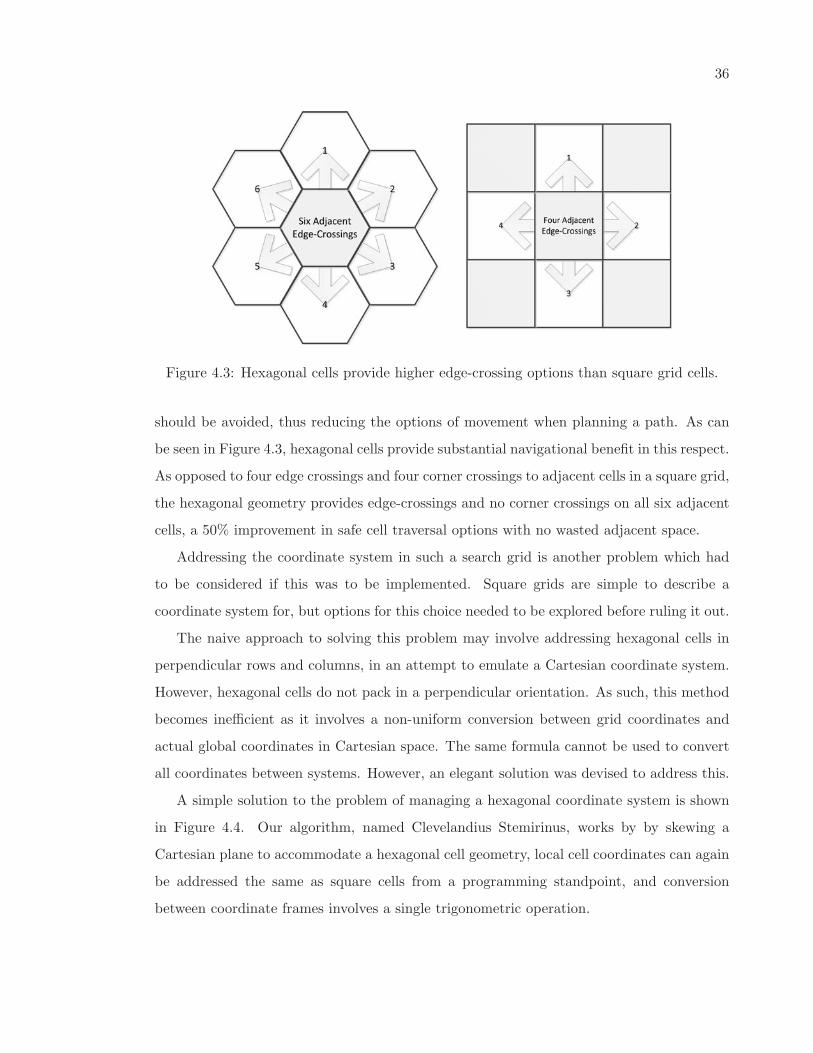
A simple solution to the problem of managing a hexagonal coordinate system is shown
in Figure 4.4. Our algorithm, named Clevelandius Stemirinus, works by by skewing a
Cartesian plane to accommodate a hexagonal cell geometry, local cell coordinates can again
be addressed the same as square cells from a programming standpoint, and conversion
between coordinate frames involves a single trigonometric operation.
37
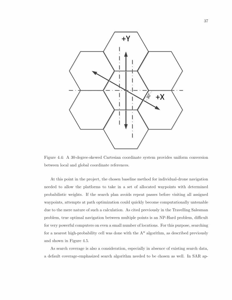
Figure 4.4: A 30-degree-skewed Cartesian coordinate system provides uniform conversion
between local and global coordinate references.
At this point in the project, the chosen baseline method for individual-drone navigation
needed to allow the platforms to take in a set of allocated waypoints with determined
probabilistic weights. If the search plan avoids repeat passes before visiting all assigned
waypoints, attempts at path optimization could quickly become computationally untenable
due to the mere nature of such a calculation. As cited previously in the Travelling Salesman
problem, true optimal navigation between multiple points is an NP-Hard problem, difficult
for very powerful computers on even a small number of locations. For this purpose, searching
for a nearest high-probability cell was done with the A* algorithm, as described previously
and shown in Figure 4.5.
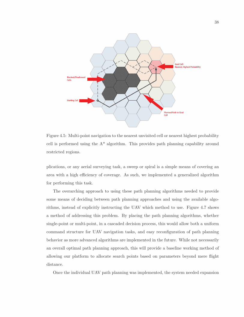
As search coverage is also a consideration, especially in absence of existing search data,
a default coverage-emphasized search algorithm needed to be chosen as well. In SAR ap-
38
Figure 4.5: Multi-point navigation to the nearest unvisited cell or nearest highest probability
cell is performed using the A* algorithm. This provides path planning capability around
restricted regions.
plications, or any aerial surveying task, a sweep or spiral is a simple means of covering an
area with a high efficiency of coverage. As such, we implemented a generalized algorithm
for performing this task.
The overarching approach to using these path planning algorithms needed to provide
some means of deciding between path planning approaches and using the available algo-
rithms, instead of explicitly instructing the UAV which method to use. Figure 4.7 shows
a method of addressing this problem. By placing the path planning algorithms, whether
single-point or multi-point, in a cascaded decision process, this would allow both a uniform
command structure for UAV navigation tasks, and easy reconfiguration of path planning
behavior as more advanced algorithms are implemented in the future. While not necessarily
an overall optimal path planning approach, this will provide a baseline working method of
allowing our platform to allocate search points based on parameters beyond mere flight
distance.
Once the individual UAV path planning was implemented, the system needed expansion
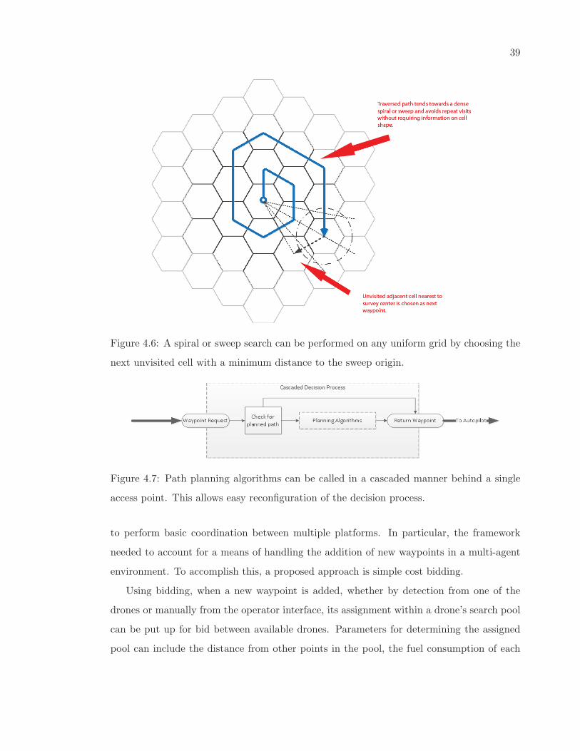
39
Figure 4.6: A spiral or sweep search can be performed on any uniform grid by choosing the
next unvisited cell with a minimum distance to the sweep origin.
Figure 4.7: Path planning algorithms can be called in a cascaded manner behind a single
access point. This allows easy reconfiguration of the decision process.
to perform basic coordination between multiple platforms. In particular, the framework
needed to account for a means of handling the addition of new waypoints in a multi-agent
environment. To accomplish this, a proposed approach is simple cost bidding.
Using bidding, when a new waypoint is added, whether by detection from one of the
drones or manually from the operator interface, its assignment within a drone’s search pool
can be put up for bid between available drones. Parameters for determining the assigned
pool can include the distance from other points in the pool, the fuel consumption of each
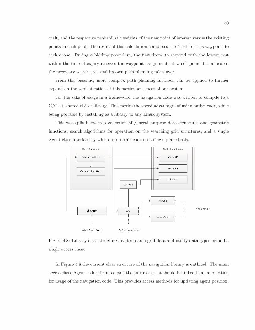
40
craft, and the respective probabilistic weights of the new point of interest versus the existing
points in each pool. The result of this calculation comprises the ”cost” of this waypoint to
each drone. During a bidding procedure, the first drone to respond with the lowest cost
within the time of expiry receives the waypoint assignment, at which point it is allocated
the necessary search area and its own path planning takes over.
From this baseline, more complex path planning methods can be applied to further
expand on the sophistication of this particular aspect of our system.
For the sake of usage in a framework, the navigation code was written to compile to a
C/C++ shared object library. This carries the speed advantages of using native code, while
being portable by installing as a library to any Linux system.
This was split between a collection of general purpose data structures and geometric
functions, search algorithms for operation on the searching grid structures, and a single
Agent class interface by which to use this code on a single-plane basis.
Figure 4.8: Library class structure divides search grid data and utility data types behind a
single access class.
In Figure 4.8 the current class structure of the navigation library is outlined. The main
access class, Agent, is for the most part the only class that should be linked to an application
for usage of the navigation code. This provides access methods for updating agent position,
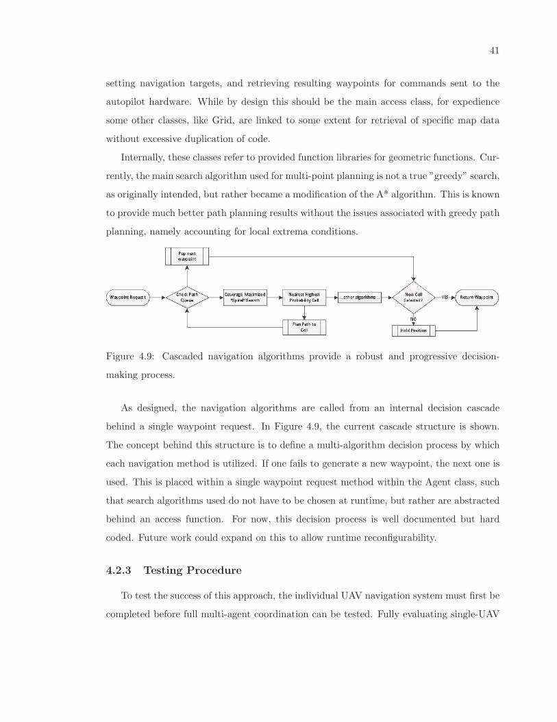
41
setting navigation targets, and retrieving resulting waypoints for commands sent to the
autopilot hardware. While by design this should be the main access class, for expedience
some other classes, like Grid, are linked to some extent for retrieval of specific map data
without excessive duplication of code.
Internally, these classes refer to provided function libraries for geometric functions. Cur-
rently, the main search algorithm used for multi-point planning is not a true ”greedy” search,
as originally intended, but rather became a modification of the A* algorithm. This is known
to provide much better path planning results without the issues associated with greedy path
planning, namely accounting for local extrema conditions.
Figure 4.9: Cascaded navigation algorithms provide a robust and progressive decision-
making process.
As designed, the navigation algorithms are called from an internal decision cascade
behind a single waypoint request. In Figure 4.9, the current cascade structure is shown.
The concept behind this structure is to define a multi-algorithm decision process by which
each navigation method is utilized. If one fails to generate a new waypoint, the next one is
used. This is placed within a single waypoint request method within the Agent class, such
that search algorithms used do not have to be chosen at runtime, but rather are abstracted
behind an access function. For now, this decision process is well documented but hard
coded. Future work could expand on this to allow runtime reconfigurability.
4.2.3 Testing Procedure
To test the success of this approach, the individual UAV navigation system must first be
completed before full multi-agent coordination can be tested. Fully evaluating single-UAV
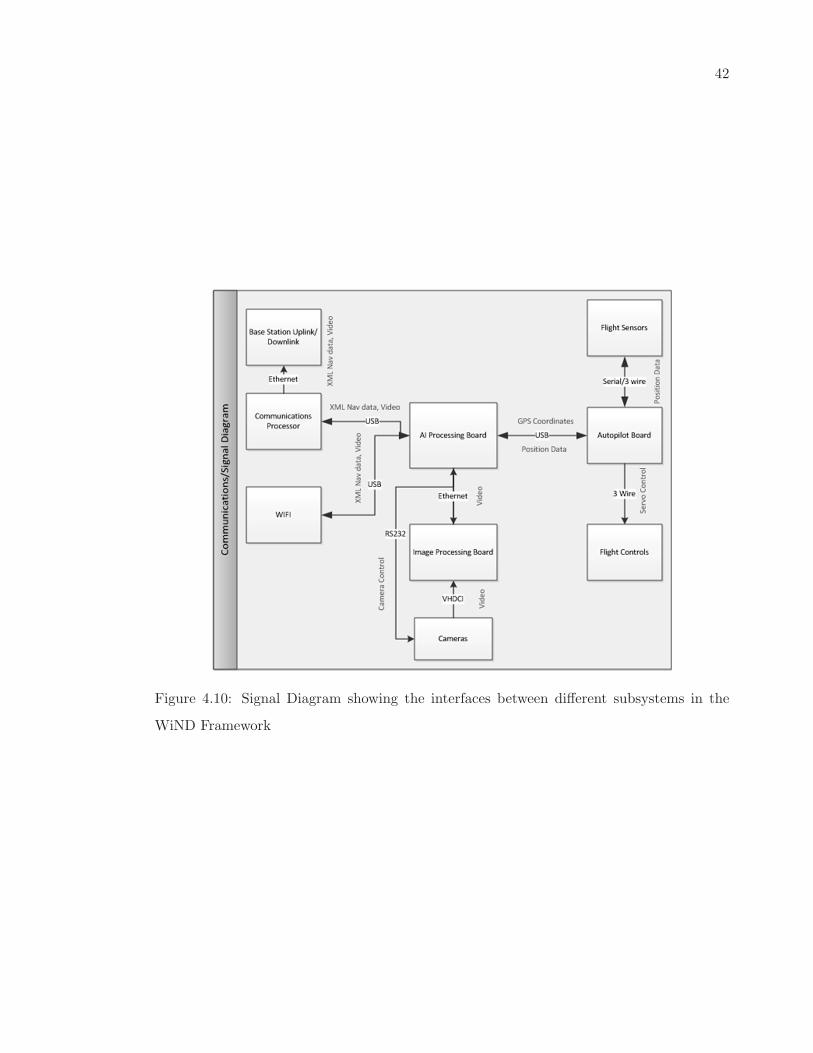
42
Figure 4.10: Signal Diagram showing the interfaces between different subsystems in the
WiND Framework
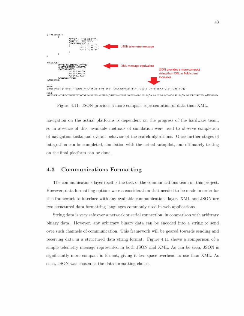
43
Figure 4.11: JSON provides a more compact representation of data than XML.
navigation on the actual platforms is dependent on the progress of the hardware team,
so in absence of this, available methods of simulation were used to observe completion
of navigation tasks and overall behavior of the search algorithms. Once further stages of
integration can be completed, simulation with the actual autopilot, and ultimately testing
on the final platform can be done.
4.3 Communications Formatting
The communications layer itself is the task of the communications team on this project.
However, data formatting options were a consideration that needed to be made in order for
this framework to interface with any available communications layer. XML and JSON are
two structured data formatting languages commonly used in web applications.
String data is very safe over a network or serial connection, in comparison with arbitrary
binary data. However, any arbitrary binary data can be encoded into a string to send
over such channels of communication. This framework will be geared towards sending and
receiving data in a structured data string format. Figure 4.11 shows a comparison of a
simple telemetry message represented in both JSON and XML. As can be seen, JSON is
significantly more compact in format, giving it less space overhead to use than XML. As
such, JSON was chosen as the data formatting choice.
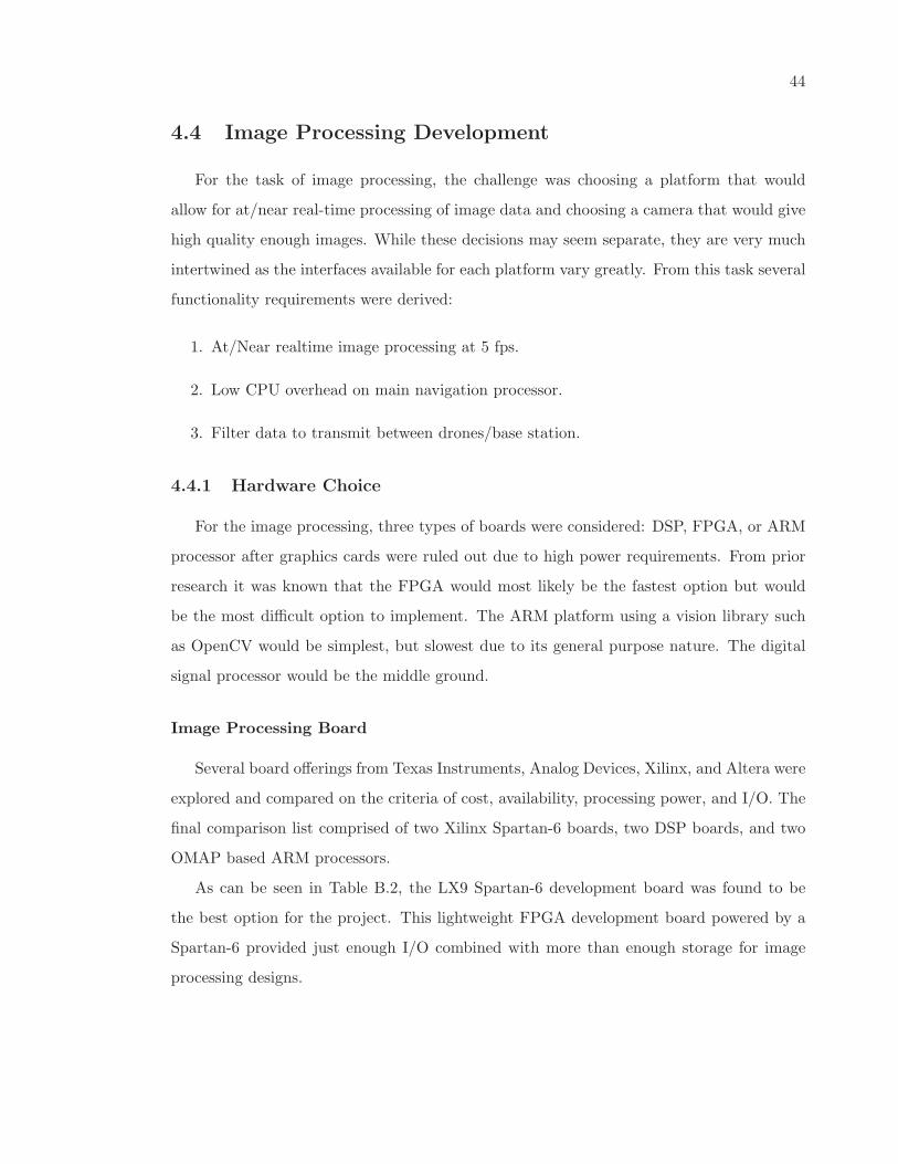
44
4.4 Image Processing Development
For the task of image processing, the challenge was choosing a platform that would
allow for at/near real-time processing of image data and choosing a camera that would give
high quality enough images. While these decisions may seem separate, they are very much
intertwined as the interfaces available for each platform vary greatly. From this task several
functionality requirements were derived:
1. At/Near realtime image processing at 5 fps.
2. Low CPU overhead on main navigation processor.
3. Filter data to transmit between drones/base station.
4.4.1 Hardware Choice
For the image processing, three types of boards were considered: DSP, FPGA, or ARM
processor after graphics cards were ruled out due to high power requirements. From prior
research it was known that the FPGA would most likely be the fastest option but would
be the most difficult option to implement. The ARM platform using a vision library such
as OpenCV would be simplest, but slowest due to its general purpose nature. The digital
signal processor would be the middle ground.
Image Processing Board
Several board offerings from Texas Instruments, Analog Devices, Xilinx, and Altera were
explored and compared on the criteria of cost, availability, processing power, and I/O. The
final comparison list comprised of two Xilinx Spartan-6 boards, two DSP boards, and two
OMAP based ARM processors.
As can be seen in Table B.2, the LX9 Spartan-6 development board was found to be
the best option for the project. This lightweight FPGA development board powered by a
Spartan-6 provided just enough I/O combined with more than enough storage for image
processing designs.
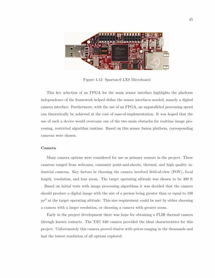
45
Figure 4.12: Spartan-6 LX9 Microboard
This key selection of an FPGA for the main sensor interface highlights the platform
independence of the framework helped define the sensor interfaces needed, namely a digital
camera interface. Furthermore, with the use of an FPGA, an unparalleled processing speed
can theoretically be achieved at the cost of ease-of-implementation. It was hoped that the
use of such a device would overcome one of the two main obstacles for realtime image pro-
cessing, restricted algorithm runtime. Based on this sensor fusion platform, corresponding
cameras were chosen.
Camera
Many camera options were considered for use as primary sensors in the project. These
cameras ranged from webcams, consumer point-and-shoots, thermal, and high quality in-
dustrial cameras. Key factors in choosing the camera involved field-of-view (FOV), focal
length, resolution, and lens zoom. The target operating altitude was chosen to be 400 ft
. Based on initial tests with image processing algorithms it was decided that the camera
should produce a digital image with the size of a person being greater than or equal to 100
px2 at the target operating altitude. This size requirement could be met by either choosing
a camera with a larger resolution, or choosing a camera with greater zoom.
Early in the project development there was hope for obtaining a FLIR thermal camera
through known contacts. The TAU 640 camera provided the ideal characteristics for this
project. Unfortunately this camera proved elusive with prices ranging in the thousands and
had the lowest resolution of all options explored.
46
Initial research also found the possibility of remote controlling high-end consumer(DSLR)
cameras. An opensource software program, “GPhoto,” running in linux allows for this ca-
pability. As with the thermal cameras, cost proved a major barrier in addition to increased
weight, increased size, and decreased flexibility. This type of system would have the addi-
tional requirements of running linux and It was for these reasons that this class was similarly
ruled out.
Typical webcams have low to high resolution specifications with relatively low zoom
capability. For example, the Microsoft LifeCam Cinema has a resolution of 1280x720 pixels
with a field of view of 73◦ [37]. Using simple trigonometry, at 400 ft this results in a person
being 24 px2 as seen in Figure 4.13. In addition to the size of a person in frame being
smaller than the cut-off,the problem in using such a high resolution camera is higher data
rate and higher bandwidth. As most webcams stacked up similarly, or worse, this prospect
was dismissed.
Figure 4.13: Calculation of person size (in pixels) based on altitude and FOV [7]
For interfacing with FPGAs, industrial cameras proved to the most flexible and suited
for this task. Offering a wide range of digital and analog options and a dizzying array of
performance options, this was the ultimate choice for the project. While the ultimate goal
was to have a digital video feed directly into the FPGA, an analog version of the Sony
“Block Cam,” the FCB-IX45C, was chosen do to its cheap price and performance. With
a serial controlled 18x optical and 4x digital zoom the camera could operate in the full
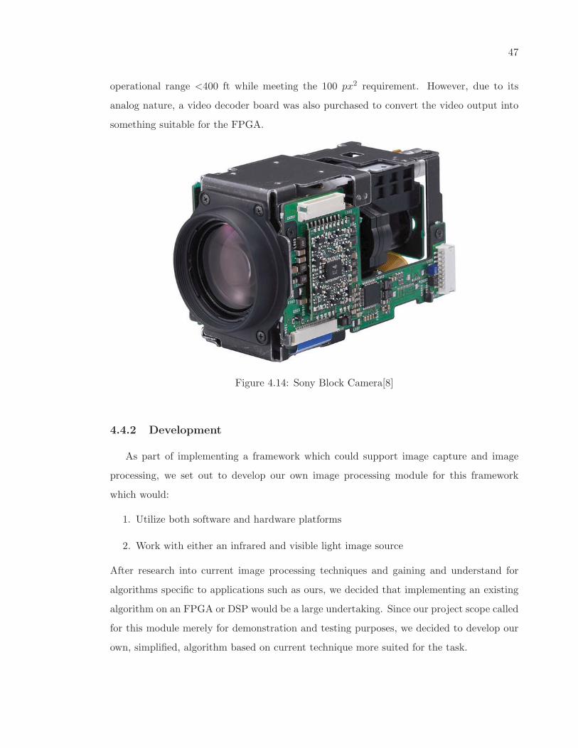
47
operational range <400 ft while meeting the 100 px2 requirement. However, due to its
analog nature, a video decoder board was also purchased to convert the video output into
something suitable for the FPGA.
Figure 4.14: Sony Block Camera[8]
4.4.2 Development
As part of implementing a framework which could support image capture and image
processing, we set out to develop our own image processing module for this framework
which would:
1. Utilize both software and hardware platforms
2. Work with either an infrared and visible light image source
After research into current image processing techniques and gaining and understand for
algorithms specific to applications such as ours, we decided that implementing an existing
algorithm on an FPGA or DSP would be a large undertaking. Since our project scope called
for this module merely for demonstration and testing purposes, we decided to develop our
own, simplified, algorithm based on current technique more suited for the task.
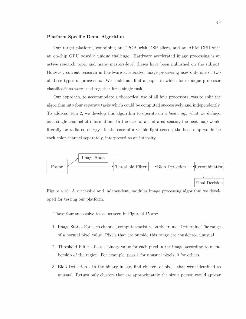
48
Platform Specific Demo Algorithm
Our target platform, containing an FPGA with DSP slices, and an ARM CPU with
an on-chip GPU posed a unique challenge. Hardware accelerated image processing is an
active research topic and many masters-level theses have been published on the subject.
However, current research in hardware accelerated image processing uses only one or two
of these types of processors. We could not find a paper in which four unique processor
classifications were used together for a single task.
Our approach, to accommodate a theoretical use of all four processors, was to split the
algorithm into four separate tasks which could be computed successively and independently.
To address item 2, we develop this algorithm to operate on a heat map, what we defined
as a single channel of information. In the case of an infrared sensor, the heat map would
literally be radiated energy. In the case of a visible light sensor, the heat map would be
each color channel separately, interpreted as an intensity.
Frame
Image Stats
�����
Threshold Filter
��Blob Detection �Recombination
Final Decision
� �
Figure 4.15: A successive and independent, modular image processing algorithm we devel-
oped for testing our platform.
These four successive tasks, as seen in Figure 4.15 are:
1. Image Stats - For each channel, compute statistics on the frame. Determine The range
of a normal pixel value. Pixels that are outside this range are considered unusual.
2. Threshold Filter - Pass a binary value for each pixel in the image according to mem-
bership of the region. For example, pass 1 for unusual pixels, 0 for others.
3. Blob Detection - In the binary image, find clusters of pixels that were identified as
unusual. Return only clusters that are approximately the size a person would appear
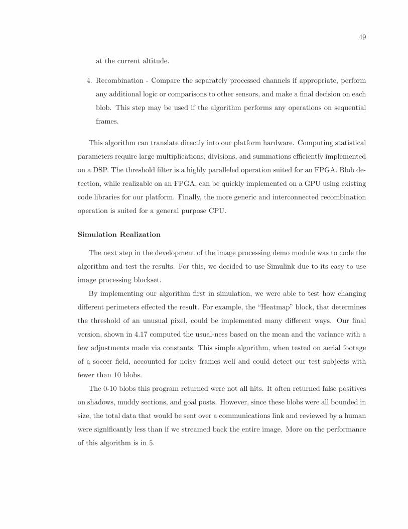
49
at the current altitude.
4. Recombination - Compare the separately processed channels if appropriate, perform
any additional logic or comparisons to other sensors, and make a final decision on each
blob. This step may be used if the algorithm performs any operations on sequential
frames.
This algorithm can translate directly into our platform hardware. Computing statistical
parameters require large multiplications, divisions, and summations efficiently implemented
on a DSP. The threshold filter is a highly paralleled operation suited for an FPGA. Blob de-
tection, while realizable on an FPGA, can be quickly implemented on a GPU using existing
code libraries for our platform. Finally, the more generic and interconnected recombination
operation is suited for a general purpose CPU.
Simulation Realization
The next step in the development of the image processing demo module was to code the
algorithm and test the results. For this, we decided to use Simulink due to its easy to use
image processing blockset.
By implementing our algorithm first in simulation, we were able to test how changing
different perimeters effected the result. For example, the “Heatmap” block, that determines
the threshold of an unusual pixel, could be implemented many different ways. Our final
version, shown in 4.17 computed the usual-ness based on the mean and the variance with a
few adjustments made via constants. This simple algorithm, when tested on aerial footage
of a soccer field, accounted for noisy frames well and could detect our test subjects with
fewer than 10 blobs.
The 0-10 blobs this program returned were not all hits. It often returned false positives
on shadows, muddy sections, and goal posts. However, since these blobs were all bounded in
size, the total data that would be sent over a communications link and reviewed by a human
were significantly less than if we streamed back the entire image. More on the performance
of this algorithm is in 5.

50
Figure 4.16: Simulink implementation of our custom image processing algorithm showing
manual adjustments. This easily adjustable model was used to fine-tune the algorithm.
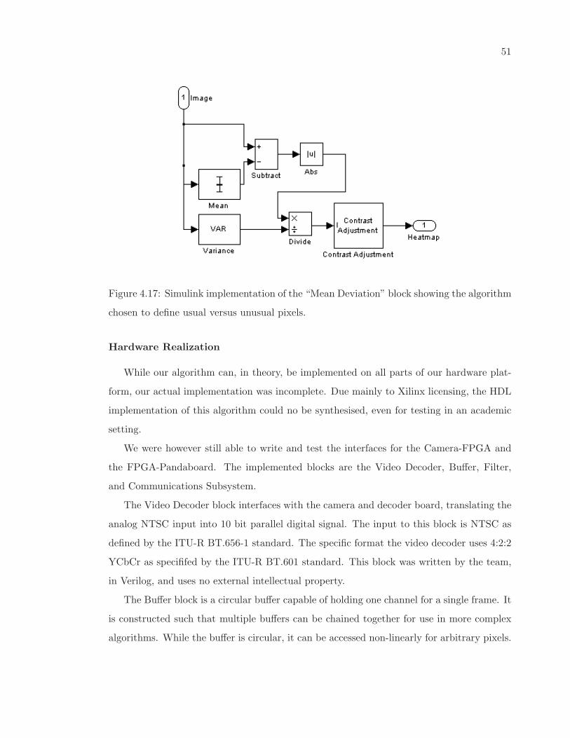
51
Figure 4.17: Simulink implementation of the “Mean Deviation” block showing the algorithm
chosen to define usual versus unusual pixels.
Hardware Realization
While our algorithm can, in theory, be implemented on all parts of our hardware plat-
form, our actual implementation was incomplete. Due mainly to Xilinx licensing, the HDL
implementation of this algorithm could no be synthesised, even for testing in an academic
setting.
We were however still able to write and test the interfaces for the Camera-FPGA and
the FPGA-Pandaboard. The implemented blocks are the Video Decoder, Buffer, Filter,
and Communications Subsystem.
The Video Decoder block interfaces with the camera and decoder board, translating the
analog NTSC input into 10 bit parallel digital signal. The input to this block is NTSC as
defined by the ITU-R BT.656-1 standard. The specific format the video decoder uses 4:2:2
YCbCr as specififed by the ITU-R BT.601 standard. This block was written by the team,
in Verilog, and uses no external intellectual property.
The Buffer block is a circular buffer capable of holding one channel for a single frame. It
is constructed such that multiple buffers can be chained together for use in more complex
algorithms. While the buffer is circular, it can be accessed non-linearly for arbitrary pixels.
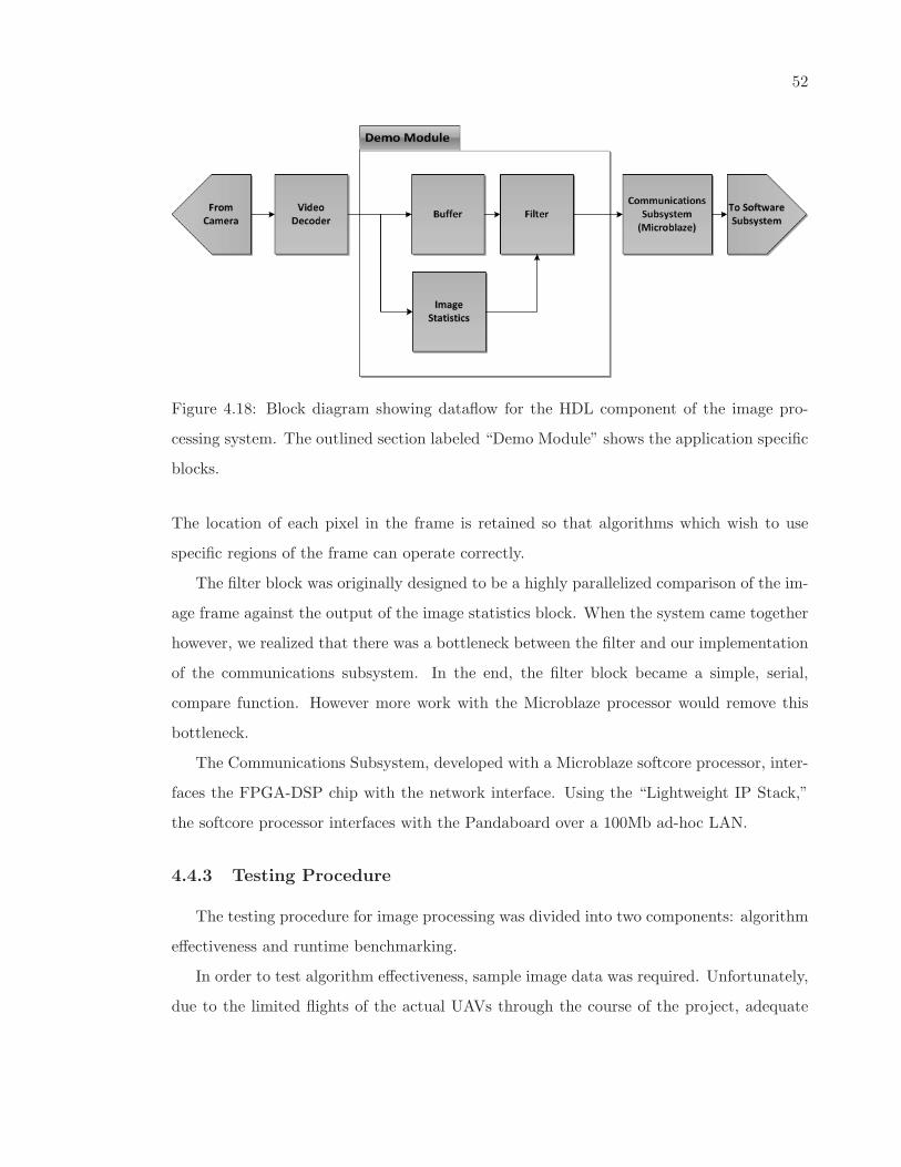
52
Figure 4.18: Block diagram showing dataflow for the HDL component of the image pro-
cessing system. The outlined section labeled “Demo Module” shows the application specific
blocks.
The location of each pixel in the frame is retained so that algorithms which wish to use
specific regions of the frame can operate correctly.
The filter block was originally designed to be a highly parallelized comparison of the im-
age frame against the output of the image statistics block. When the system came together
however, we realized that there was a bottleneck between the filter and our implementation
of the communications subsystem. In the end, the filter block became a simple, serial,
compare function. However more work with the Microblaze processor would remove this
bottleneck.
The Communications Subsystem, developed with a Microblaze softcore processor, inter-
faces the FPGA-DSP chip with the network interface. Using the “Lightweight IP Stack,”
the softcore processor interfaces with the Pandaboard over a 100Mb ad-hoc LAN.
4.4.3 Testing Procedure
The testing procedure for image processing was divided into two components: algorithm
effectiveness and runtime benchmarking.
In order to test algorithm effectiveness, sample image data was required. Unfortunately,
due to the limited flights of the actual UAVs through the course of the project, adequate
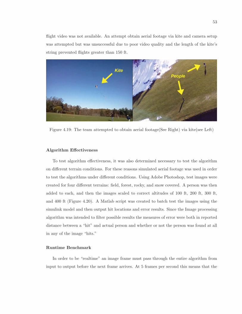
53
flight video was not available. An attempt obtain aerial footage via kite and camera setup
was attempted but was unsuccessful due to poor video quality and the length of the kite’s
string prevented flights greater than 150 ft.
Figure 4.19: The team attempted to obtain aerial footage(See Right) via kite(see Left)
Algorithm Effectiveness
To test algorithm effectiveness, it was also determined necessary to test the algorithm
on different terrain conditions. For these reasons simulated aerial footage was used in order
to test the algorithms under different conditions. Using Adobe Photoshop, test images were
created for four different terrains: field, forest, rocky, and snow covered. A person was then
added to each, and then the images scaled to correct altitudes of 100 ft, 200 ft, 300 ft,
and 400 ft (Figure 4.20). A Matlab script was created to batch test the images using the
simulink model and then output hit locations and error results. Since the Image processing
algorithm was intended to filter possible results the measures of error were both in reported
distance between a “hit” and actual person and whether or not the person was found at all
in any of the image “hits.”
Runtime Benchmark
In order to be “realtime” an image frame must pass through the entire algorithm from
input to output before the next frame arrives. At 5 frames per second this means that the
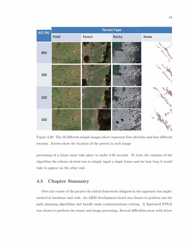
54
Figure 4.20: The 16 different sample images above represent four altitudes and four different
terrains. Arrows show the location of the person in each image
processing of a frame must take place in under 0.20 seconds. To tests the runtime of the
algorithm the scheme devised was to simply input a single frame and see how long it would
take to appear on the other end.
4.5 Chapter Summary
Over the course of the project the initial framework designed in the approach was imple-
mented in hardware and code. An ARM development board was chosen to perform run the
path planning algorithms and handle main communications routing. A Spartan-6 FPGA
was chosen to perform the sensor and image processing. Several difficulties arose with driver
55
issues and proprietary cores but were worked around. With the implementation complete,
testing was able to commence.
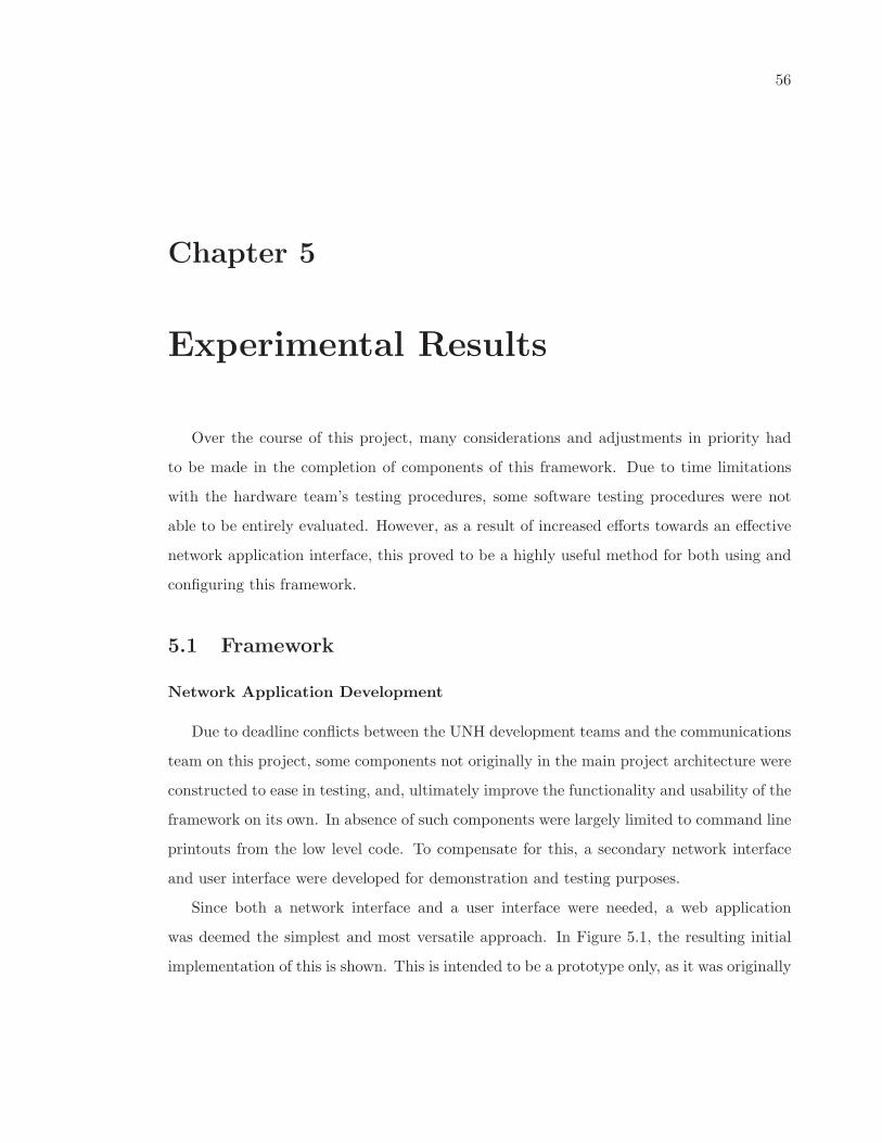
56
Chapter 5
Experimental Results
Over the course of this project, many considerations and adjustments in priority had
to be made in the completion of components of this framework. Due to time limitations
with the hardware team’s testing procedures, some software testing procedures were not
able to be entirely evaluated. However, as a result of increased efforts towards an effective
network application interface, this proved to be a highly useful method for both using and
configuring this framework.
5.1 Framework
Network Application Development
Due to deadline conflicts between the UNH development teams and the communications
team on this project, some components not originally in the main project architecture were
constructed to ease in testing, and, ultimately improve the functionality and usability of the
framework on its own. In absence of such components were largely limited to command line
printouts from the low level code. To compensate for this, a secondary network interface
and user interface were developed for demonstration and testing purposes.
Since both a network interface and a user interface were needed, a web application
was deemed the simplest and most versatile approach. In Figure 5.1, the resulting initial
implementation of this is shown. This is intended to be a prototype only, as it was originally
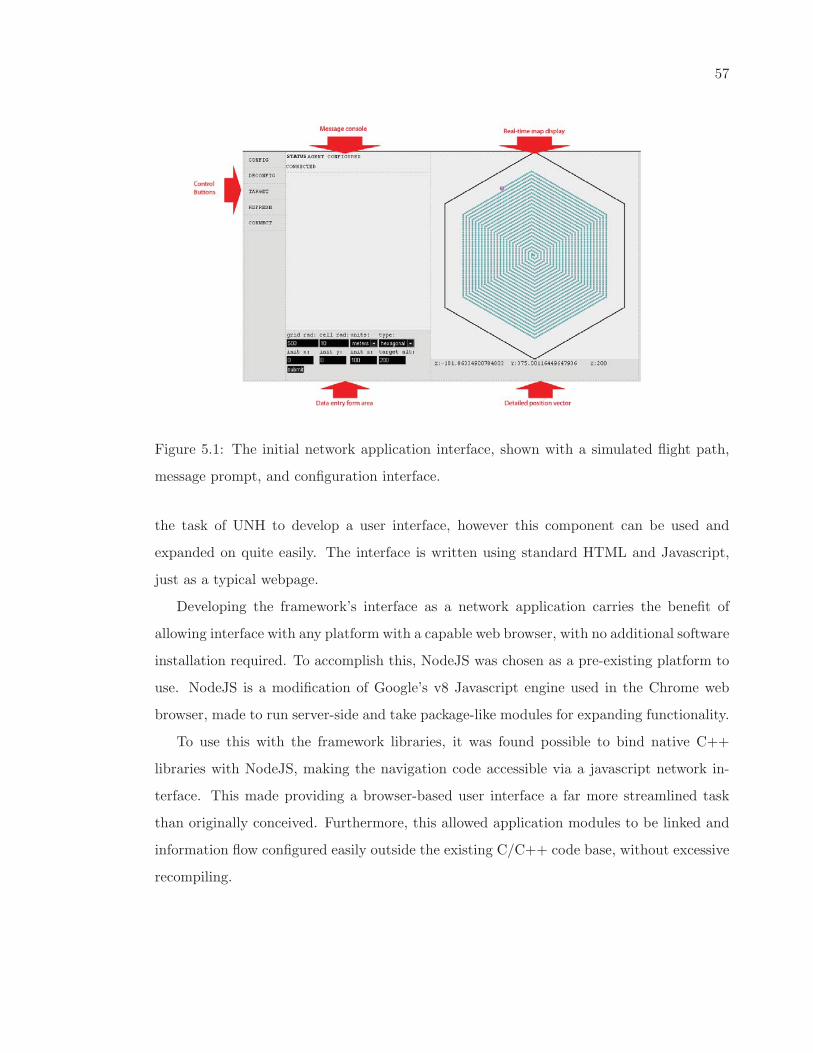
57
Figure 5.1: The initial network application interface, shown with a simulated flight path,
message prompt, and configuration interface.
the task of UNH to develop a user interface, however this component can be used and
expanded on quite easily. The interface is written using standard HTML and Javascript,
just as a typical webpage.
Developing the framework’s interface as a network application carries the benefit of
allowing interface with any platform with a capable web browser, with no additional software
installation required. To accomplish this, NodeJS was chosen as a pre-existing platform to
use. NodeJS is a modification of Google’s v8 Javascript engine used in the Chrome web
browser, made to run server-side and take package-like modules for expanding functionality.
To use this with the framework libraries, it was found possible to bind native C++
libraries with NodeJS, making the navigation code accessible via a javascript network in-
terface. This made providing a browser-based user interface a far more streamlined task
than originally conceived. Furthermore, this allowed application modules to be linked and
information flow configured easily outside the existing C/C++ code base, without excessive
recompiling.
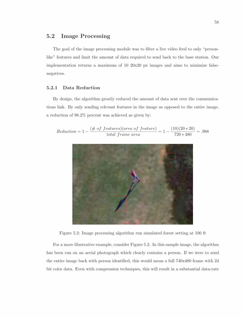
58
5.2 Image Processing
The goal of the image processing module was to filter a live video feed to only “person-
like” features and limit the amount of data required to send back to the base station. Our
implementation returns a maximum of 10 20x20 px images and aims to minimize false-
negatives.
5.2.1 Data Reduction
By design, the algorithm greatly reduced the amount of data sent over the communica-
tions link. By only sending relevant features in the image as opposed to the entire image,
a reduction of 98.2% percent was achieved as given by:
Reduction = 1− (# of features)(area of feature)
total frame area= 1− (10)(20 ∗ 20)
720 ∗ 480 = .988
Figure 5.2: Image processing algorithm run simulated forest setting at 100 ft
For a more illustrative example, consider Figure 5.2. In this sample image, the algorithm
has been run on an aerial photograph which clearly contains a person. If we were to send
the entire image back with person identified, this would mean a full 740x480 frame with 24
bit color data. Even with compression techniques, this will result in a substantial data-rate
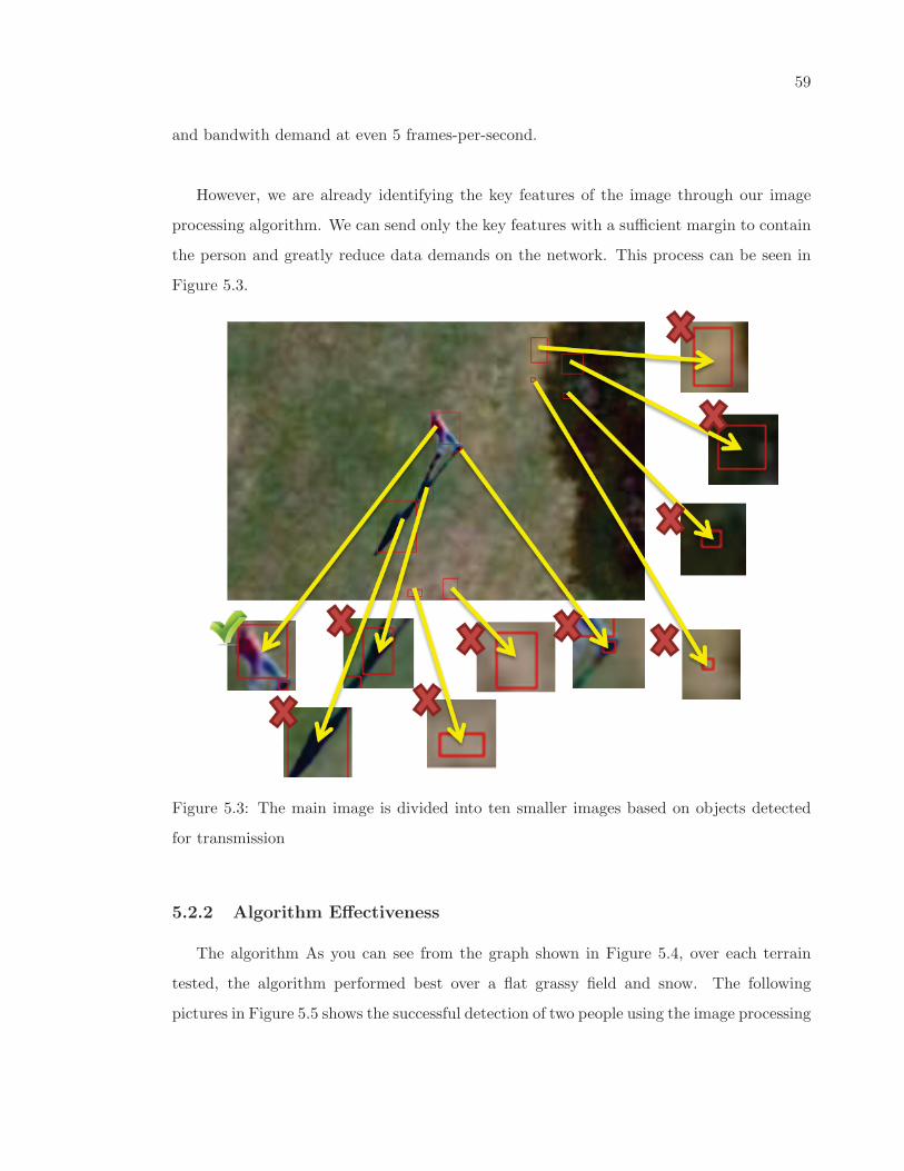
59
and bandwith demand at even 5 frames-per-second.
However, we are already identifying the key features of the image through our image
processing algorithm. We can send only the key features with a sufficient margin to contain
the person and greatly reduce data demands on the network. This process can be seen in
Figure 5.3.
Figure 5.3: The main image is divided into ten smaller images based on objects detected
for transmission
5.2.2 Algorithm Effectiveness
The algorithm As you can see from the graph shown in Figure 5.4, over each terrain
tested, the algorithm performed best over a flat grassy field and snow. The following
pictures in Figure 5.5 shows the successful detection of two people using the image processing
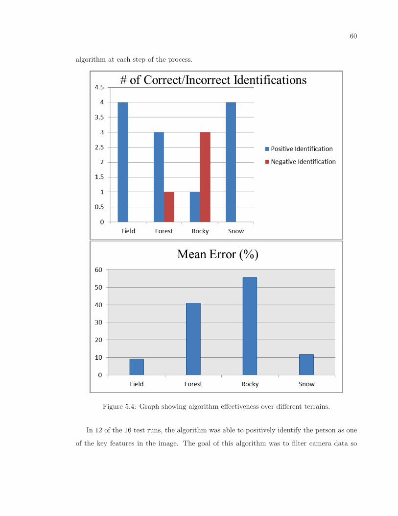
60
algorithm at each step of the process.
Figure 5.4: Graph showing algorithm effectiveness over different terrains.
In 12 of the 16 test runs, the algorithm was able to positively identify the person as one
of the key features in the image. The goal of this algorithm was to filter camera data so
61
that only “person-like” features would be returned to the user. Because the algorithm was
able to do this in the majority of test cases we deem that our implementation was fairly
successful. The test results, with bounding boxes highlighted can be found in the Appendix.
As can be seen from the data, the algorithm had the most trouble dealing with the “rocky
terrain.” Logically, this cluttered environment proved to be the least ideal backdrop. When
operating under such conditions the base algorithm would benefit from several tweaks such
as more filtering and a higher threshold to remove the unwanted noise. Combining data
from multiple passes and multiple sensors would also improve performance but were unable
to be tested. However, to have much chance of success, the victims would need to head for
clearings in the forest to be detected reliably.
These theoretical results show the necessity for adequate camera equipment and justify
the decision to purchase a camera with more zoom capabilities. Through further testing
on actual aerial footage the “sweet-spot” of zoom could be determined for the algorithm.
Armed with this knowledge, accuracy could further be improved as the camera can vary its
zoom based on altitude to achieve this.
5.2.3 Hardware Implementation
Unfortunately, the hardware implementation of the image processing algorithm was not
fully completed in the span of the project. The FPGA was successfully linked with the
video decoder board allowing video input. In addition, a softcore microblaze processor
was successfully implemented with custom peripherals to interface with the image process-
ing components and Pandaboard via ethernet and the light weight IP stack. The image
processing component itself was not able to be tested due to issues with discussed in Im-
plementation.
5.2.4 Runtime Benchmark
The team was unsuccessful in creating a runtime benchmark due to difficulties with
development tools.
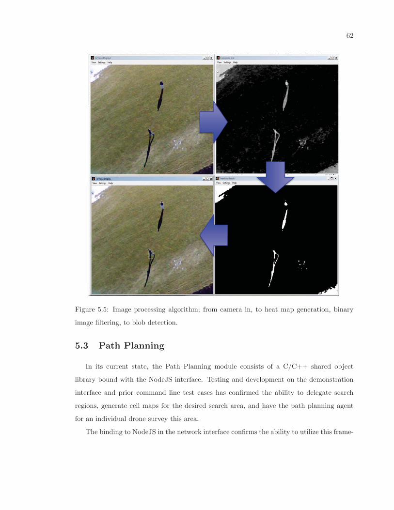
62
Figure 5.5: Image processing algorithm; from camera in, to heat map generation, binary
image filtering, to blob detection.
5.3 Path Planning
In its current state, the Path Planning module consists of a C/C++ shared object
library bound with the NodeJS interface. Testing and development on the demonstration
interface and prior command line test cases has confirmed the ability to delegate search
regions, generate cell maps for the desired search area, and have the path planning agent
for an individual drone survey this area.
The binding to NodeJS in the network interface confirms the ability to utilize this frame-
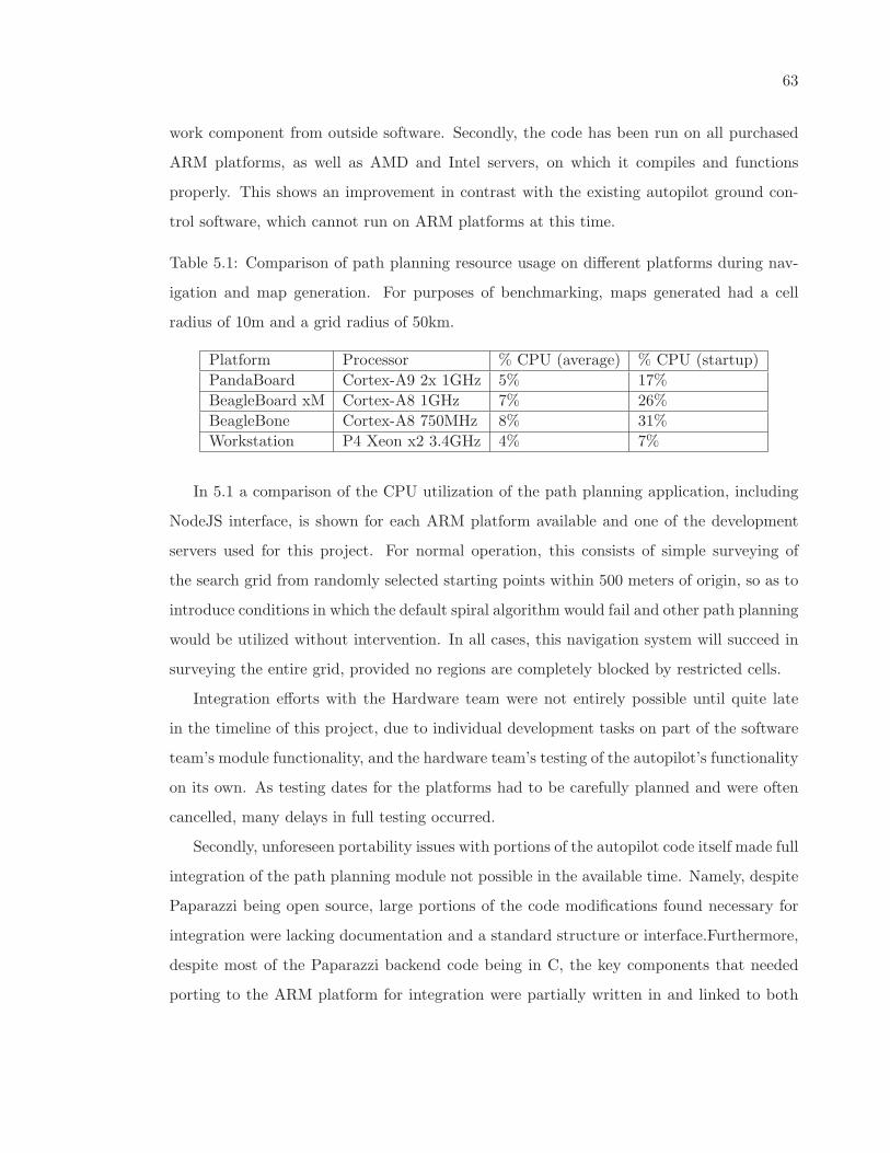
63
work component from outside software. Secondly, the code has been run on all purchased
ARM platforms, as well as AMD and Intel servers, on which it compiles and functions
properly. This shows an improvement in contrast with the existing autopilot ground con-
trol software, which cannot run on ARM platforms at this time.
Table 5.1: Comparison of path planning resource usage on different platforms during nav-
igation and map generation. For purposes of benchmarking, maps generated had a cell
radius of 10m and a grid radius of 50km.
Platform Processor % CPU (average) % CPU (startup)
PandaBoard Cortex-A9 2x 1GHz 5% 17%
BeagleBoard xM Cortex-A8 1GHz 7% 26%
BeagleBone Cortex-A8 750MHz 8% 31%
Workstation P4 Xeon x2 3.4GHz 4% 7%
In 5.1 a comparison of the CPU utilization of the path planning application, including
NodeJS interface, is shown for each ARM platform available and one of the development
servers used for this project. For normal operation, this consists of simple surveying of
the search grid from randomly selected starting points within 500 meters of origin, so as to
introduce conditions in which the default spiral algorithm would fail and other path planning
would be utilized without intervention. In all cases, this navigation system will succeed in
surveying the entire grid, provided no regions are completely blocked by restricted cells.
Integration efforts with the Hardware team were not entirely possible until quite late
in the timeline of this project, due to individual development tasks on part of the software
team’s module functionality, and the hardware team’s testing of the autopilot’s functionality
on its own. As testing dates for the platforms had to be carefully planned and were often
cancelled, many delays in full testing occurred.
Secondly, unforeseen portability issues with portions of the autopilot code itself made full
integration of the path planning module not possible in the available time. Namely, despite
Paparazzi being open source, large portions of the code modifications found necessary for
integration were lacking documentation and a standard structure or interface.Furthermore,
despite most of the Paparazzi backend code being in C, the key components that needed
porting to the ARM platform for integration were partially written in and linked to both
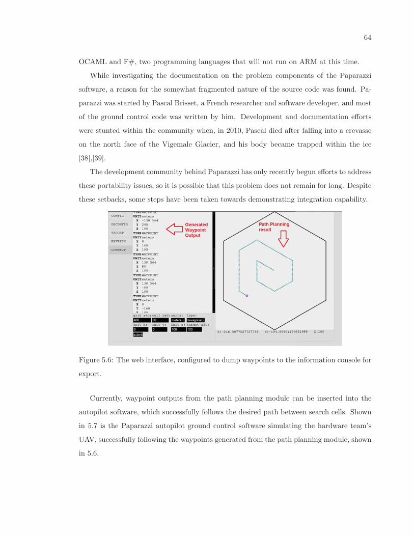
64
OCAML and F#, two programming languages that will not run on ARM at this time.
While investigating the documentation on the problem components of the Paparazzi
software, a reason for the somewhat fragmented nature of the source code was found. Pa-
parazzi was started by Pascal Brisset, a French researcher and software developer, and most
of the ground control code was written by him. Development and documentation efforts
were stunted within the community when, in 2010, Pascal died after falling into a crevasse
on the north face of the Vigemale Glacier, and his body became trapped within the ice
[38],[39].
The development community behind Paparazzi has only recently begun efforts to address
these portability issues, so it is possible that this problem does not remain for long. Despite
these setbacks, some steps have been taken towards demonstrating integration capability.
Figure 5.6: The web interface, configured to dump waypoints to the information console for
export.
Currently, waypoint outputs from the path planning module can be inserted into the
autopilot software, which successfully follows the desired path between search cells. Shown
in 5.7 is the Paparazzi autopilot ground control software simulating the hardware team’s
UAV, successfully following the waypoints generated from the path planning module, shown
in 5.6.
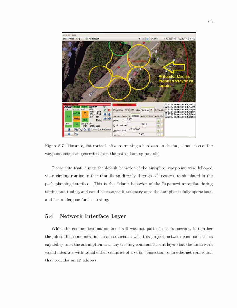
65
Figure 5.7: The autopilot control software running a hardware-in-the-loop simulation of the
waypoint sequence generated from the path planning module.
Please note that, due to the default behavior of the autopilot, waypoints were followed
via a circling routine, rather than flying directly through cell centers, as simulated in the
path planning interface. This is the default behavior of the Paparazzi autopilot during
testing and tuning, and could be changed if necessary once the autopilot is fully operational
and has undergone further testing.
5.4 Network Interface Layer
While the communications module itself was not part of this framework, but rather
the job of the communications team associated with this project, network communications
capability took the assumption that any existing communications layer that the framework
would integrate with would either comprise of a serial connection or an ethernet connection
that provides an IP address.
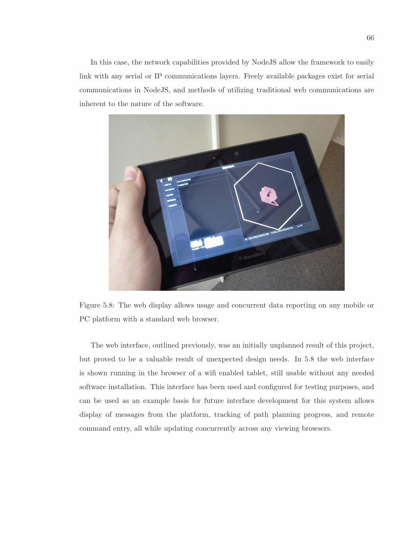
66
In this case, the network capabilities provided by NodeJS allow the framework to easily
link with any serial or IP communications layers. Freely available packages exist for serial
communications in NodeJS, and methods of utilizing traditional web communications are
inherent to the nature of the software.
Figure 5.8: The web display allows usage and concurrent data reporting on any mobile or
PC platform with a standard web browser.
The web interface, outlined previously, was an initially unplanned result of this project,
but proved to be a valuable result of unexpected design needs. In 5.8 the web interface
is shown running in the browser of a wifi enabled tablet, still usable without any needed
software installation. This interface has been used and configured for testing purposes, and
can be used as an example basis for future interface development for this system allows
display of messages from the platform, tracking of path planning progress, and remote
command entry, all while updating concurrently across any viewing browsers.
67
5.5 Development Platforms
In order to perform development and testing on the actual hardware, it had to first be
setup in a usable development environment. This required installing an configuring a stable
Linux distribution with the desired software installations to meet our needs.
For the most part, the only non-standard software we wished to test on this platform was
OpenCV. Since image processing is to be implemented on the coprocessor board itself, this is
not an absolutely vital functionality, the ability to handle high-level calculations, command
processing, and data logging/reporting and path planning are the primary purpose of this
board.
5.5.1 Development Environment Setup
The PandaBoard community website has three primarily recommended operating sys-
tems for the Pandaboard; Ubuntu, Android, and a minimal validation-only installation,
based off of Angstrom.
Initial installation attempts were made with Ubuntu, however performance was slower
than expected. Various alternative installations were found, including ARM-optimized
builds developed from the Linaro foundation.
Illustrated in Figure 5.9 is an early testing configuration, with a minimal Ubuntu server
installation and a light window manager. As can be seen in the diagram, this setup was
used for initial package configuration and testing of image capture capabilities. The window
manager chosen for this build was OpenBox, shown on both the main display, along with
a networked VNC display shown on the laptop monitor. The usage of a networked VNC
display confirmed some image capture capabilities, along with providing a relatively smooth
image update speed over the network.
Unfortunately, stability issues and graphics incompatibility demanded exploration of
alternative distributions. Ubuntu’s startup time, even with minimal graphics installed, was
unacceptably slow, and attempts to integrate existing proprietary graphics drivers were met
with errors, such as system instability and graphics elements not rendering properly.
Alternative Linux installations largely proved to be geared towards Android development
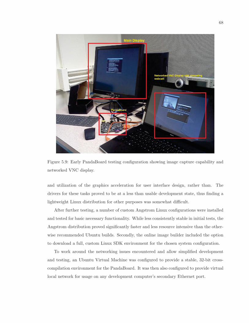
68
Figure 5.9: Early PandaBoard testing configuration showing image capture capability and
networked VNC display.
and utilization of the graphics acceleration for user interface design, rather than. The
drivers for these tasks proved to be at a less than usable development state, thus finding a
lightweight Linux distribution for other purposes was somewhat difficult.
After further testing, a number of custom Angstrom Linux configurations were installed
and tested for basic necessary functionality. While less consistently stable in initial tests, the
Angstrom distribution proved significantly faster and less resource intensive than the other-
wise recommended Ubuntu builds. Secondly, the online image builder included the option
to download a full, custom Linux SDK environment for the chosen system configuration.
To work around the networking issues encountered and allow simplified development
and testing, an Ubuntu Virtual Machine was configured to provide a stable, 32-bit cross-
compilation environment for the PandaBoard. It was then also configured to provide virtual
local network for usage on any development computer’s secondary Ethernet port.
69
The Angstrom SDK was installed on this virtual machine along with other necessary
compilation tools. Cross compilation worked for some software components, but results
were more consistent and easier to reproduce by compiling natively on the target hardware.
During initial testing efforts on the PandaBoard, attempts were made to utilize the
graphics acceleration hardware. Despite the advertised capabilities, usability of this par-
ticular feature of the board proved to be poorly supported or documented. The demo
programs for this hardware were not able to be successfully compiled, and in the presence
of supported drivers for the hardware, some problematic secondary issues arose. Since this
was not a primary or vital component of this portion of the hardware, it was decided to not
utilize this particular capability.
Later on in development, it was found that a standard element of the ARM Cortex-A
series processors could be utilized for acceleration of some image processing or vectorized
mathematical tasks. Both the Cortex-A8 and Cortex-A9 contain a Single-Instruction Mul-
tiple Data (SIMD) core, called NEON, for performing generalized parallel operations on
arrayed datatypes. While not as potentially useful as access to the PandaBoard’s graphics
core, this particular capability is useful for precisely the types of calculations we would need
to do for color filtering or general parallel calculations.
This hardware extension is present in the processors of both the PandaBoard and all
BeagleBoard variants, as well as other hardware using the same ARM architecture. This
would make our code substantially more portable between platforms, and allow switches to
much smaller ARM-based platforms, such as the BeagleBone, with minimal code adaptation.
Initial testing with the NEON core has been done, and both native compilation and
cross compilation of NEON-targeted code appears to work. Furthermore, with careful code
organization, the GCC compiler can be made to automatically optimize some code to utilize
the processor where it otherwise would not. We plan to test implementation of some basic,
useful image operations on this, and benchmark them for comparison and future use. As of
this point, our code is not utilizing this feature, but it can be applied as appropriate.
With respect to networking issues, it was discovered upon initial tests that the Ethernet
controller for the PandaBoard and BeagleBoard lacks a dedicated, unique MAC address.
This manifests as a randomly generated MAC address on each activation of the hardware
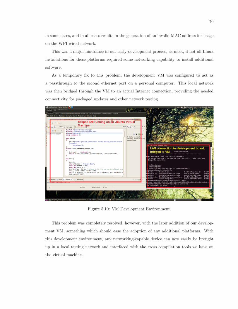
70
in some cases, and in all cases results in the generation of an invalid MAC address for usage
on the WPI wired network.
This was a major hindrance in our early development process, as most, if not all Linux
installations for these platforms required some networking capability to install additional
software.
As a temporary fix to this problem, the development VM was configured to act as
a passthrough to the second ethernet port on a personal computer. This local network
was then bridged through the VM to an actual Internet connection, providing the needed
connectivity for packaged updates and other network testing.
Figure 5.10: VM Development Environment.
This problem was completely resolved, however, with the later addition of our develop-
ment VM, something which should ease the adoption of any additional platforms. With
this development environment, any networking-capable device can now easily be brought
up in a local testing network and interfaced with the cross compilation tools we have on
the virtual machine.
71
5.5.2 AI Testing Environment
In order to prototype a user interface for our base station and provide a basis for sim-
ulation of our navigation algorithm choices, a testing application and map GUI were con-
structed within MATLAB to utilize our map and path generation algorithms. The goal of
this software was to provide a means of algorithm performance analysis using our gathered
SAR statistics and rapid-fire scenario simulations. By calculating probabilistic ”time to
completion” of our search algorithms, this would both give us a baseline for comparison,
and provide a very useful tool for any expansion on our framework.
Due to a bug within MATLAB, however, the GUI portion of this software component
was lost before much could be done with it. The entire back-end survived this, however,
allowing us to use the grid-generation algorithms developed in MATLAB in the actual
software library.
5.6 Chapter Summary
The goal of this project was the creation of a framework for search and rescue operations
with unmanned aerial vehicles. In the end, a cross-platform framework with interchangeable
modules was successfully created. Demonstration modules for image processing and path-
planning were developed. As part of this process an image processing algorithm for detecting
people in aerial footage was designed and tested with simulation data. Difficulties with
implementation prevented a fully functional hardware design. A path-planning algorithm
was created and implemented on an embedded ARM platform which was then tested with
a web-based GUI made for the project.
72
Chapter 6
Conclusion
Designing a framework to support search and rescue UAVs was a unique undertaking
that required an immense knowledge of the modular components the team aimed to accom-
modate as well as a broad understanding of the entire system for integration. An expansive
research base, delicate planning, and novel thinking contributed to achieve flexibility and
generality of the framework while maintaining SAR specific features.
In the first chapter of this report, a need is presented to reduce the cost of search and
rescue operations. To reduce the cost of SAR, the proposed approach was to use multiple,
coordinated, autonomous, unmanned aerial vehicles. An implementation, further described,
would reduce the number of people required to perform a search per unit area and thus
the total cost of SAR operations over time. This greater goal of Project WiND was then
divided into three general components, designed and implemented by three WPI teams: the
UAV platform, the wireless communications, and the software framework.
As the team working on the software framework, development efforts were two part. The
team developed a framework to accommodate modular image processing, path planning,
navigation, and communication programs. This involved understanding the needs of SAR
operators, platform developers, and the communications team, however it also required
planning for all scenarios. This pushed the framework to accommodate a design in which
all sensor processing occurred on the UAV and away from any base-station or mother-ship.
In addition to the framework, the team also developed a set of modules which use this
73
framework. These demo modules serve to demonstrate functionality and to guide future
developers who will program for and expand on this work.
6.1 Future Work
Originally, this team hoped to leave future work on this project limited to module
development, but due to many factors, portions of the framework, such as the hardware
image processing, have not been fully tested and remain un-integrated. This is unfortunate,
but provides motivation for a future team to focus more on these portions of the existing
framework for better usability and create more framework-supplied tools for developers to
use. To outline the tasks for future improvement:
• While the team did develop demo modules for image processing and navigation, initial
focus was on the framework before integrating into a deployment-ready SAR system.
The image processing modules could be significantly improved using more advanced
algorithms such as motion-detection, shadow removal, and shape recognition. More
of this system can be implemented on the FPGA-DSP, further freeing the software
processor for communications and navigation.
• The navigation modules could be improved with more AI designed specifically for
multi-agent optimizations and platform specific features. Right now, individual robot
navigation is functional, and communications capabilities allow for multi-robot coor-
dination to be implemented and tested when individual platforms are more capable.
Additions to this module could include utilizing information such as fuel consumption,
effects of weather, and terrain data to improve resource utilization.
• Something this team did not attempt was a more advanced user interface for robot
control and information feedback. The existing interface was limited to communicat-
ing data on the flight path of a single UAV as part of the testing procedure. It did
not have the ability to display information regarding multiple UAVs in coordination
or image processing data. A team at the University of New Hampshire is supposedly
working on this problem using a Microsoft Surface. However, the current state of
74
that project is unknown, and advancements in the existing web interface would make
this a more valuable framework overall, as well as ease integration if and when the
Microsoft Surface is used.
In conclusion, this project demonstrated the overall concept of a specialized framework
for search and rescue. The team successfully integrated purpose built modules into this
framework and showed general functionality. They then installed this framework onto an
ARM platform and integrated that with the hardware platform. However, full integration
and testing is unfinished given development status of both the hardware and communica-
tions platforms. The modules themselves are limited, and the hardware implementation
of image processing was not integrated due to licensing difficulties. The team accommo-
dated for a communications system successfully and implemented a custom interface as an
enhancement on the original design, but full testing on the production platforms awaits com-
pletion. With dedication, future teams can hopefully improve and finalize this framework
and release it as a field-ready development platform.
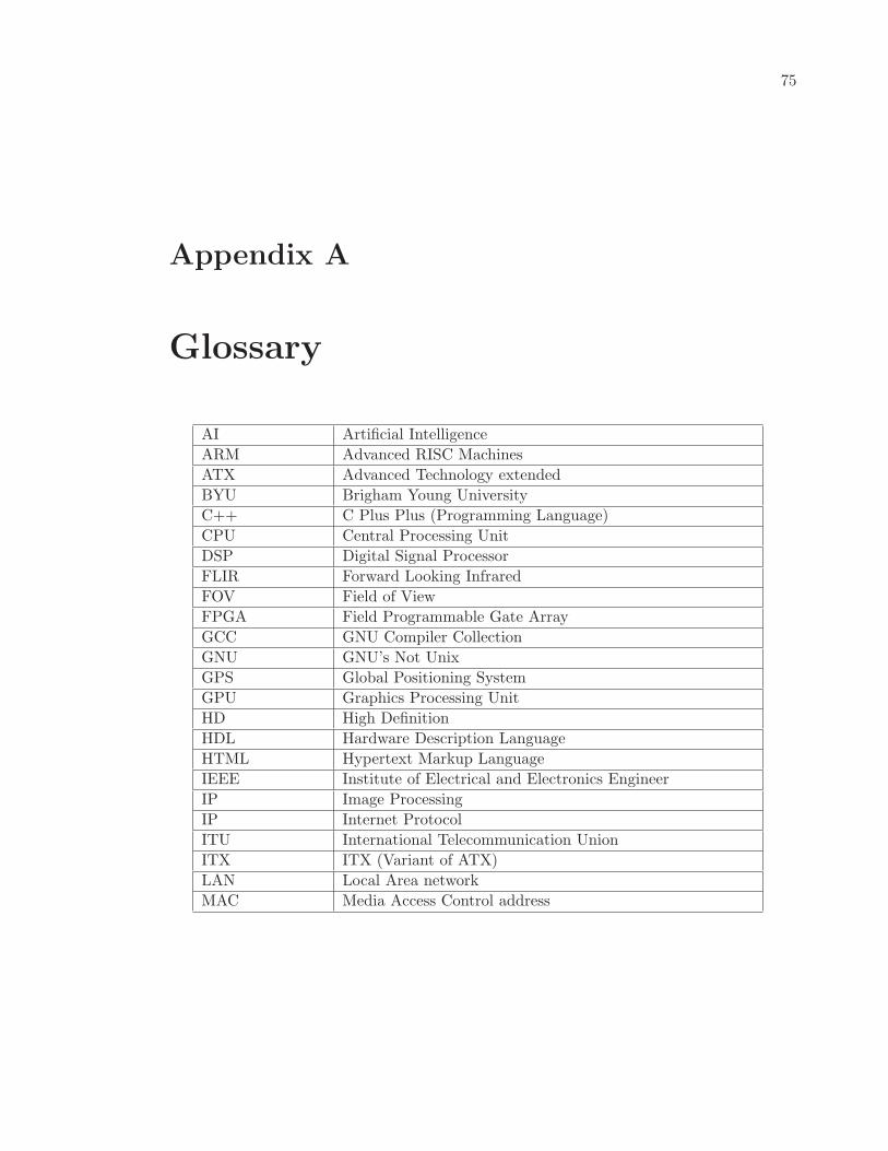
75
Appendix A
Glossary
AI Artificial Intelligence
ARM Advanced RISC Machines
ATX Advanced Technology extended
BYU Brigham Young University
C++ C Plus Plus (Programming Language)
CPU Central Processing Unit
DSP Digital Signal Processor
FLIR Forward Looking Infrared
FOV Field of View
FPGA Field Programmable Gate Array
GCC GNU Compiler Collection
GNU GNU’s Not Unix
GPS Global Positioning System
GPU Graphics Processing Unit
HD High Definition
HDL Hardware Description Language
HTML Hypertext Markup Language
IEEE Institute of Electrical and Electronics Engineer
IP Image Processing
IP Internet Protocol
ITU International Telecommunication Union
ITX ITX (Variant of ATX)
LAN Local Area network
MAC Media Access Control address
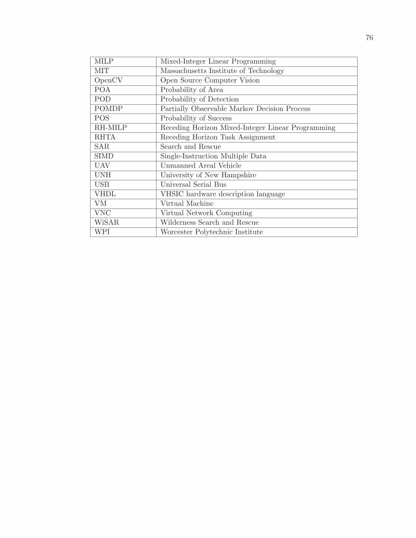
76
MILP Mixed-Integer Linear Programming
MIT Massachusetts Institute of Technology
OpenCV Open Source Computer Vision
POA Probability of Area
POD Probability of Detection
POMDP Partially Observable Markov Decision Process
POS Probability of Success
RH-MILP Receding Horizon Mixed-Integer Linear Programming
RHTA Receding Horizon Task Assignment
SAR Search and Rescue
SIMD Single-Instruction Multiple Data
UAV Unmanned Areal Vehicle
UNH University of New Hampshire
USB Universal Serial Bus
VHDL VHSIC hardware description language
VM Virtual Machine
VNC Virtual Network Computing
WiSAR Wilderness Search and Rescue
WPI Worcester Polytechnic Institute
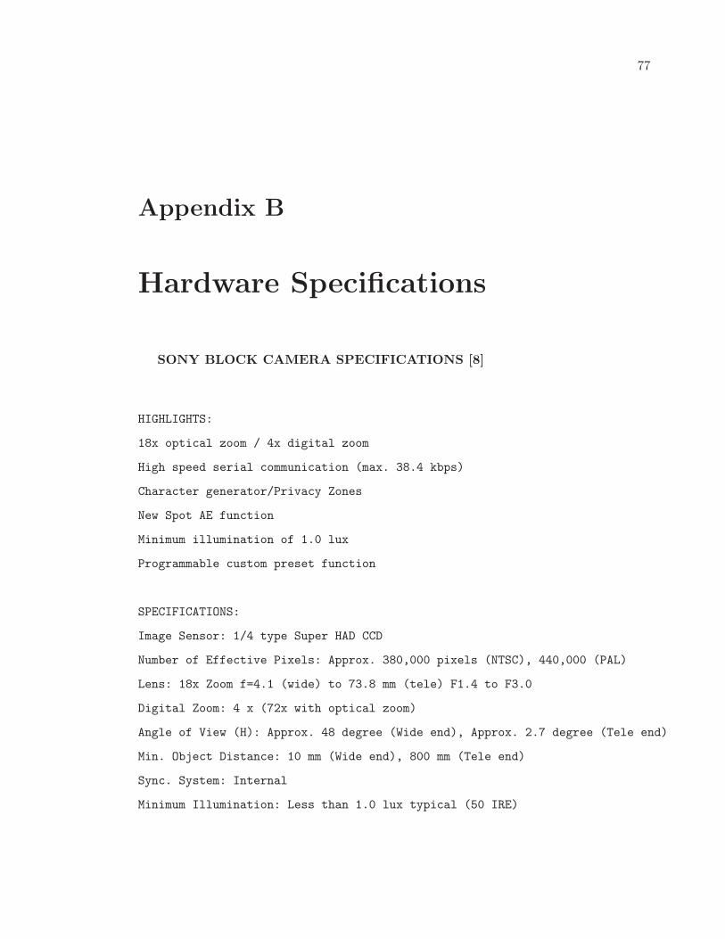
77
Appendix B
Hardware Specifications
SONY BLOCK CAMERA SPECIFICATIONS [8]
HIGHLIGHTS:
18x optical zoom / 4x digital zoom
High speed serial communication (max. 38.4 kbps)
Character generator/Privacy Zones
New Spot AE function
Minimum illumination of 1.0 lux
Programmable custom preset function
SPECIFICATIONS:
Image Sensor: 1/4 type Super HAD CCD
Number of Effective Pixels: Approx. 380,000 pixels (NTSC), 440,000 (PAL)
Lens: 18x Zoom f=4.1 (wide) to 73.8 mm (tele) F1.4 to F3.0
Digital Zoom: 4 x (72x with optical zoom)
Angle of View (H): Approx. 48 degree (Wide end), Approx. 2.7 degree (Tele end)
Min. Object Distance: 10 mm (Wide end), 800 mm (Tele end)
Sync. System: Internal
Minimum Illumination: Less than 1.0 lux typical (50 IRE)
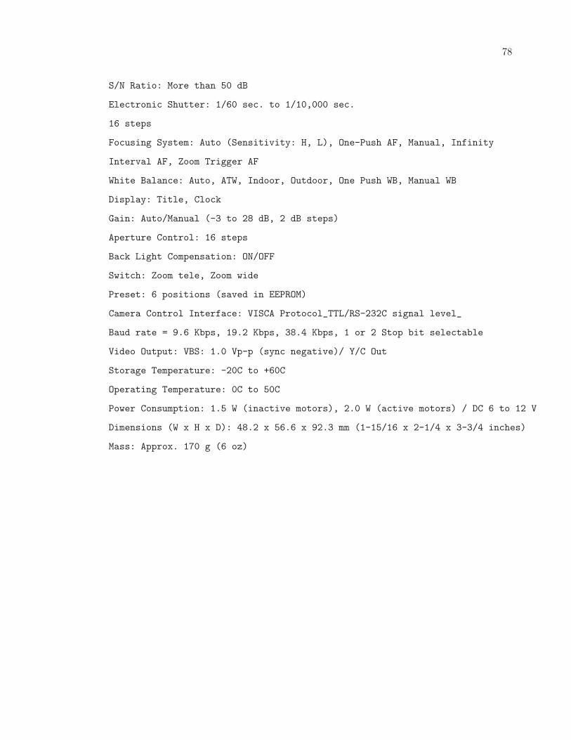
78
S/N Ratio: More than 50 dB
Electronic Shutter: 1/60 sec. to 1/10,000 sec.
16 steps
Focusing System: Auto (Sensitivity: H, L), One-Push AF, Manual, Infinity
Interval AF, Zoom Trigger AF
White Balance: Auto, ATW, Indoor, Outdoor, One Push WB, Manual WB
Display: Title, Clock
Gain: Auto/Manual (-3 to 28 dB, 2 dB steps)
Aperture Control: 16 steps
Back Light Compensation: ON/OFF
Switch: Zoom tele, Zoom wide
Preset: 6 positions (saved in EEPROM)
Camera Control Interface: VISCA Protocol_TTL/RS-232C signal level_
Baud rate = 9.6 Kbps, 19.2 Kbps, 38.4 Kbps, 1 or 2 Stop bit selectable
Video Output: VBS: 1.0 Vp-p (sync negative)/ Y/C Out
Storage Temperature: -20C to +60C
Operating Temperature: 0C to 50C
Power Consumption: 1.5 W (inactive motors), 2.0 W (active motors) / DC 6 to 12 V
Dimensions (W x H x D): 48.2 x 56.6 x 92.3 mm (1-15/16 x 2-1/4 x 3-3/4 inches)
Mass: Approx. 170 g (6 oz)
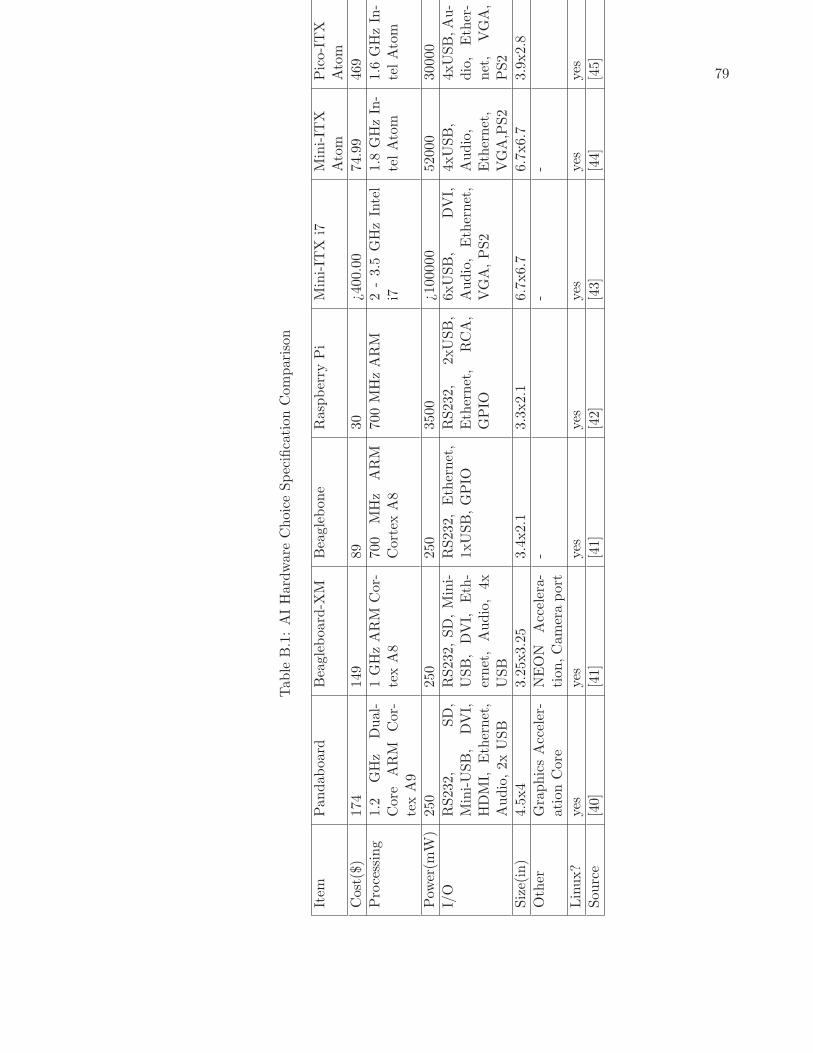
79
Table
B.1:AIHardware
ChoiceSpecificationComparison
Item
Pan
daboard
Beagleboard-X
MBeaglebone
Raspberry
Pi
Mini-IT
Xi7
Mini-IT
XAtom
Pico-ITX
Atom
Cost($)
174
149
8930
¿400.00
74.99
469
Processing
1.2
GHz
Dual-
Core
ARM
Cor-
texA9
1GHzARM
Cor-
texA8
700
MHz
ARM
Cortex
A8
700MHzARM
2-3.5
GHzIntel
i71.8
GHzIn-
telAtom
1.6
GHzIn-
telAtom
Pow
er(m
W)
250
250
250
3500
¿100
000
5200
030
000
I/O
RS232,
SD,
Mini-USB,
DVI,
HDMI,
Ethernet,
Audio,2xUSB
RS232,SD,Mini-
USB,DVI,
Eth-
ernet,Audio,4x
USB
RS232,Ethernet,
1xUSB,GPIO
RS232,
2xUSB,
Ethernet,
RCA,
GPIO
6xUSB,
DVI,
Audio,
Ethernet,
VGA,PS2
4xUSB,
Audio,
Ethernet,
VGA,PS2
4xUSB,Au-
dio,
Ether-
net,
VGA,
PS2
Size(in)
4.5x4
3.25x3.25
3.4x2.1
3.3x2.1
6.7x6.7
6.7x6.7
3.9x2.8
Other
GraphicsAcceler-
ationCore
NEON
Accelera-
tion,Cameraport
--
-
Linux?
yes
yes
yes
yes
yes
yes
yes
Source
[40]
[41]
[41]
[42]
[43]
[44]
[45]
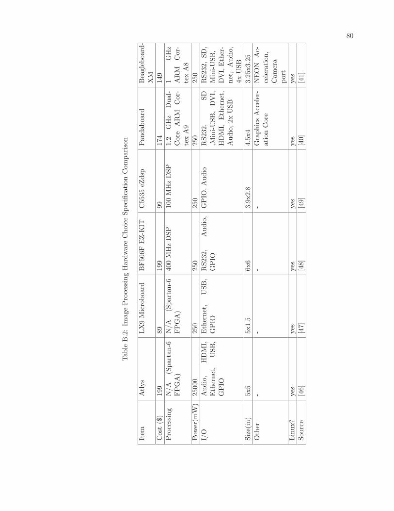
80
Tab
leB.2:Im
ageProcessingHardware
ChoiceSpecificationComparison
Item
Atlys
LX9Microboard
BF506FEZ-K
ITC5535eZ
dsp
Pan
daboard
Beagleboard-
XM
Cost
($)
199
8919
999
174
149
Processing
N/A
(Spartan-6
FPGA)
N/A
(Spartan-6
FPGA)
400MHzDSP
100MHzDSP
1.2
GHz
Dual-
Core
ARM
Cor-
texA9
1GHz
ARM
Cor-
texA8
Pow
er(m
W)
2500
025
025
025
025
025
0
I/O
Audio,
HDMI,
Ethernet,
USB,
GPIO
Ethernet,
USB,
GPIO
RS232,
Audio,
GPIO
GPIO
,Audio
RS232,
SD
,Mini-USB,
DVI,
HDMI,
Ethernet,
Audio,2xUSB
RS232,SD,
Mini-USB,
DVI,Ether-
net,Audio,
4xUSB
Size(in)
5x5
5x1.5
6x6
3.9x2.8
4.5x4
3.25x3.25
Other
--
--
GraphicsAcceler-
ationCore
NEON
Ac-
celeration,
Camera
port
Linux?
yes
yes
yes
yes
yes
yes
Source
[46]
[47]
[48]
[49]
[40]
[41]
81
Appendix C
AI Path Planning Code
1 #ifndef __AGENT_H
#define __AGENT_H
/**
* File: Agent.hpp
* Author: Jonathan Estabrook
6 * Description:
*
* Main access class for interfacing with navigation , control , and data
* acquisition functions. Effectively this is where you tell the robot
* what to do. Most high -level organizational changes in the library
11 * should happen here.
*
* NOTE ON COORDINATES:
* For purposes of differentiation "Global" refers to scaled cartesian
coordinates *relative*
* to the search grid origin , in the appropriate units , not true "Global"
in a Lat/Lon sense.
16 * "Local" refers to integer -unit coordinates for usage within the
* search grid. One local unit is scaled by the cell scaling factor for
global units.
*
* Conversions between Lat/Lon and Global are assumed to happen elsewhere
before input.
* */
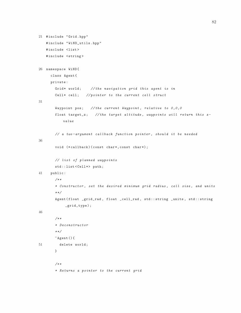
82
21 #include "Grid.hpp"
#include "WiND_utils.hpp"
#include <list >
#include <string >
26 namespace WiND{
class Agent{
private:
Grid* world; //the navigation grid this agent is in
Cell* cell; // pointer to the current cell struct
31
Waypoint pos; //the current Waypoint , relative to 0,0,0
float target_z; //the target altitude , waypoints will return this z-
value
// a two -argument callback function pointer , should it be needed
36
void (* callback)(const char*,const char*);
// list of planned waypoints
std::list <Cell*> path;
41 public:
/**
* Constructor , set the desired minimum grid radius , cell size , and units
**/
Agent(float _grid_rad , float _cell_rad , std:: string _units , std:: string
_grid_type);
46
/**
* Deconstructor
**/
~Agent(){
51 delete world;
}
/**
* Returns a pointer to the current grid
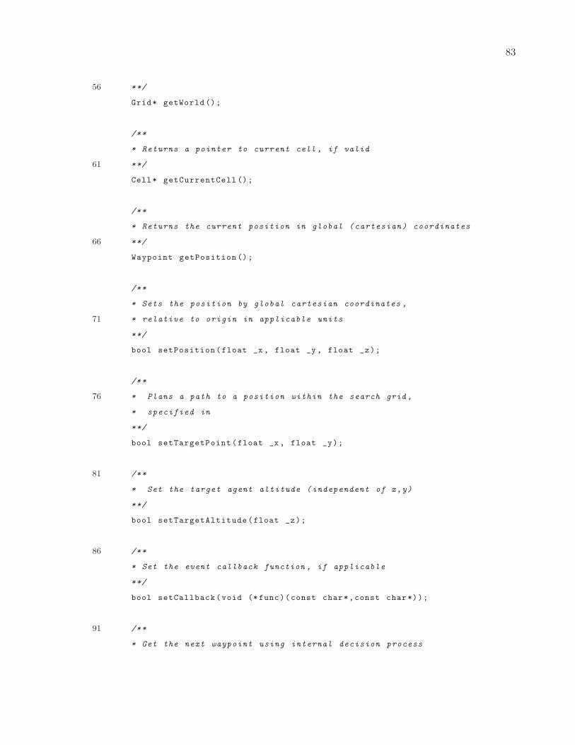
83
56 **/
Grid* getWorld ();
/**
* Returns a pointer to current cell , if valid
61 **/
Cell* getCurrentCell ();
/**
* Returns the current position in global (cartesian) coordinates
66 **/
Waypoint getPosition ();
/**
* Sets the position by global cartesian coordinates ,
71 * relative to origin in applicable units
**/
bool setPosition(float _x, float _y, float _z);
/**
76 * Plans a path to a position within the search grid ,
* specified in
**/
bool setTargetPoint(float _x, float _y);
81 /**
* Set the target agent altitude (independent of x,y)
**/
bool setTargetAltitude(float _z);
86 /**
* Set the event callback function , if applicable
**/
bool setCallback(void (*func)(const char*,const char*));
91 /**
* Get the next waypoint using internal decision process
84
**/
Waypoint getNextWaypoint ();
};
96 }
#endif /* __AGENT_H */
/**
2 * File: Agent.cpp
* Author: Jonathan Estabrook
* Description:
*
* Main access class for interfacing with navigation , control , and data
7 * acquisition functions. Effectively this is where you tell the robot
* what to do. Most high -level organizational changes in the library
* should happen here.
*
* NOTE ON COORDINATES:
12 * For purposes of differentiation "Global" refers to scaled cartesian
coordinates *relative*
* to the search grid origin , in the appropriate units , not true "Global"
in a Lat/Lon sense.
* "Local" refers to integer -unit coordinates for usage within the
* search grid. One local unit is scaled by the cell scaling factor for
global units.
*
17 * Conversions between Lat/Lon and Global are assumed to happen elsewhere
before input.
* */
#include "Agent.hpp"
#include "HexGrid.hpp" //we’re using this locally , Agent.h doesn ’t need it
22
#include "WiND_search.hpp"
#include <list >
#include <set >
85
27 #include <algorithm >
#include <iostream > //TODO
#include <exception >
namespace WiND
{
32 Agent ::Agent(float _grid_rad , float _cell_rad , std:: string _units , std::
string _grid_type){
if(_grid_type == "hexagon")
{
this ->world = new HexGrid ();
} else {
37 throw;
}
this ->world ->init(_grid_rad ,_cell_rad ,_units);
this ->cell = NULL; // indicates uninitialized position
this ->callback = NULL; // uninitialized callback
42 }
/**
* Returns pointer to Grid
*/
47 Grid* Agent :: getWorld (){
return this ->world;
}
52 Cell* Agent :: getCurrentCell (){
return this ->cell;
}
Waypoint Agent :: getPosition (){
57 return this ->pos;
}
/**
* Set position in global cartesian units , relative to 0,0,0
62 * if the position isn’t in -world , return false
86
*/
bool Agent :: setPosition(float x, float y, float z){
// update current waypoint
this ->pos.x = x; this ->pos.y = y; this ->pos.z = z;
67 if(callback)callback("UPDATE","position updated");
Vector2D gCoords = {x,y};
//find current cell coordinates
std::pair <int ,int > lCoords = this ->world ->global_2_local(gCoords);
72 //get current cell
this ->cell = this ->world ->getCell(lCoords.first ,lCoords.second);
//if it is a valid cell , set the visited flag
if(this ->cell){ this ->cell ->visited = true; return true;}
else return false;
77 }
bool Agent :: setTargetPoint(float _x, float _y){
//first check if this is a valid point
Vector2D v = {_x,_y};
82 std::pair <int ,int > lCoords = this ->world ->global_2_local(v);
Cell* c = this ->world ->getCell(lCoords.first ,lCoords.second);
if(!c) return false;
else if(c == this ->cell) return true;
else
87 {
this ->path = planPath(this ->cell ,c,this ->world);
}
}
92 bool Agent :: setTargetAltitude(float _z)
{
this ->target_z = _z;
return true;
}
97
bool Agent :: setCallback(void (*func)(const char*, const char*))
{
87
this ->callback = func;
return (func != NULL);
102 }
/* ***************************************************************
* Interface method for single -cell search algorithms
**/
107 Waypoint Agent :: getNextWaypoint (){
// declare pointer to next cell
Cell* next = NULL;
// first check for pre -planned cells
112 if(!(this ->path.empty ()))
{
next = path.front ();
path.pop_front ();
if(callback)callback("STATUS","popping path waypoint!");
117 }
// algorithms are chained by priority
// these pick the next cell , in two dimensions , altitude is separate
// attempt using center -spiral method
122 next = next?next:getNextSpiral(this ->cell , this ->world);
// if this fails , attempt using A*, starting a planned path
// to the next unvisited cell
if(!next)
127 {
Cell* target = getNextUnvisited(this ->cell , this ->world);
this ->path = target?planPath(this ->cell ,target ,this ->world):path;
if(!(this ->path.empty ())){
next = path.front ();
132 path.pop_front ();
}
}
// Final sanity check , in the case that we are in a blocked region
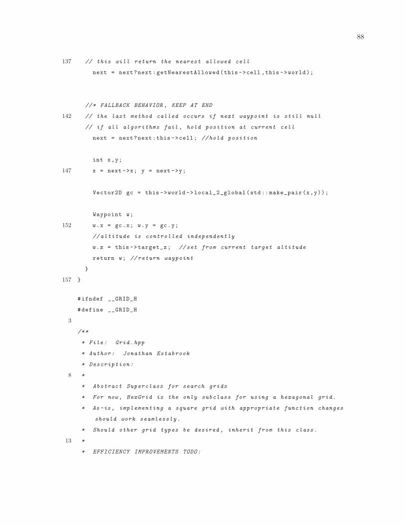
88
137 // this will return the nearest allowed cell
next = next?next:getNearestAllowed(this ->cell ,this ->world);
//* FALLBACK BEHAVIOR , KEEP AT END
142 // the last method called occurs if next waypoint is still null
// if all algorithms fail , hold position at current cell
next = next?next:this ->cell; //hold position
int x,y;
147 x = next ->x; y = next ->y;
Vector2D gc = this ->world ->local_2_global(std:: make_pair(x,y));
Waypoint w;
152 w.x = gc.x; w.y = gc.y;
// altitude is controlled independently
w.z = this ->target_z; //set from current target altitude
return w; // return waypoint
}
157 }
#ifndef __GRID_H
#define __GRID_H
3
/**
* File: Grid.hpp
* Author: Jonathan Estabrook
* Description:
8 *
* Abstract Superclass for search grids
* For now , HexGrid is the only subclass for using a hexagonal grid.
* As-is, implementing a square grid with appropriate function changes
should work seamlessly.
* Should other grid types be desired , inherit from this class.
13 *
* EFFICIENCY IMPROVEMENTS TODO:
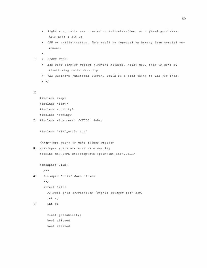
89
* Right now , cells are created on initialization , at a fixed grid size.
This uses a bit of
* CPU on initialization. This could be improved by having them created on -
demand.
*
18 * OTHER TODO:
* Add some simpler region blocking methods. Right now , this is done by
disallowing cells directly.
* The geometry functions library would be a good thing to use for this.
* */
23
#include <map >
#include <list >
#include <utility >
#include <string >
28 #include <iostream > //TODO: debug
#include "WiND_utils.hpp"
//map -type macro to make things quicker
33 // integer pairs are used as a map key
#define MAP_TYPE std::map <std::pair <int ,int >,Cell >
namespace WiND{
/**
38 * Simple "cell" data struct
**/
struct Cell{
//local grid coordinates (signed integer pair key)
int x;
43 int y;
float probability;
bool allowed;
bool visited;
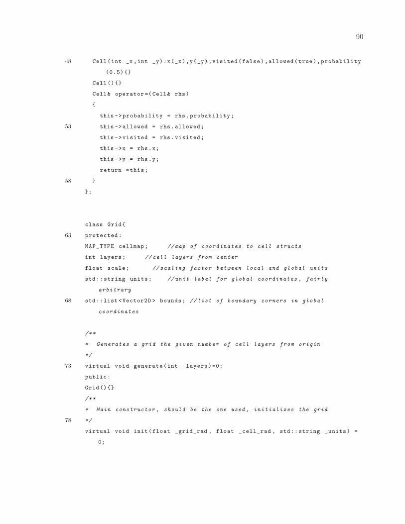
90
48 Cell(int _x ,int _y):x(_x),y(_y),visited(false),allowed(true),probability
(0.5){}
Cell(){}
Cell& operator =(Cell& rhs)
{
this ->probability = rhs.probability;
53 this ->allowed = rhs.allowed;
this ->visited = rhs.visited;
this ->x = rhs.x;
this ->y = rhs.y;
return *this;
58 }
};
class Grid{
63 protected:
MAP_TYPE cellmap; //map of coordinates to cell structs
int layers; //cell layers from center
float scale; // scaling factor between local and global units
std:: string units; //unit label for global coordinates , fairly
arbitrary
68 std::list <Vector2D > bounds; //list of boundary corners in global
coordinates
/**
* Generates a grid the given number of cell layers from origin
*/
73 virtual void generate(int _layers)=0;
public:
Grid(){}
/**
* Main constructor , should be the one used , initializes the grid
78 */
virtual void init(float _grid_rad , float _cell_rad , std:: string _units) =
0;
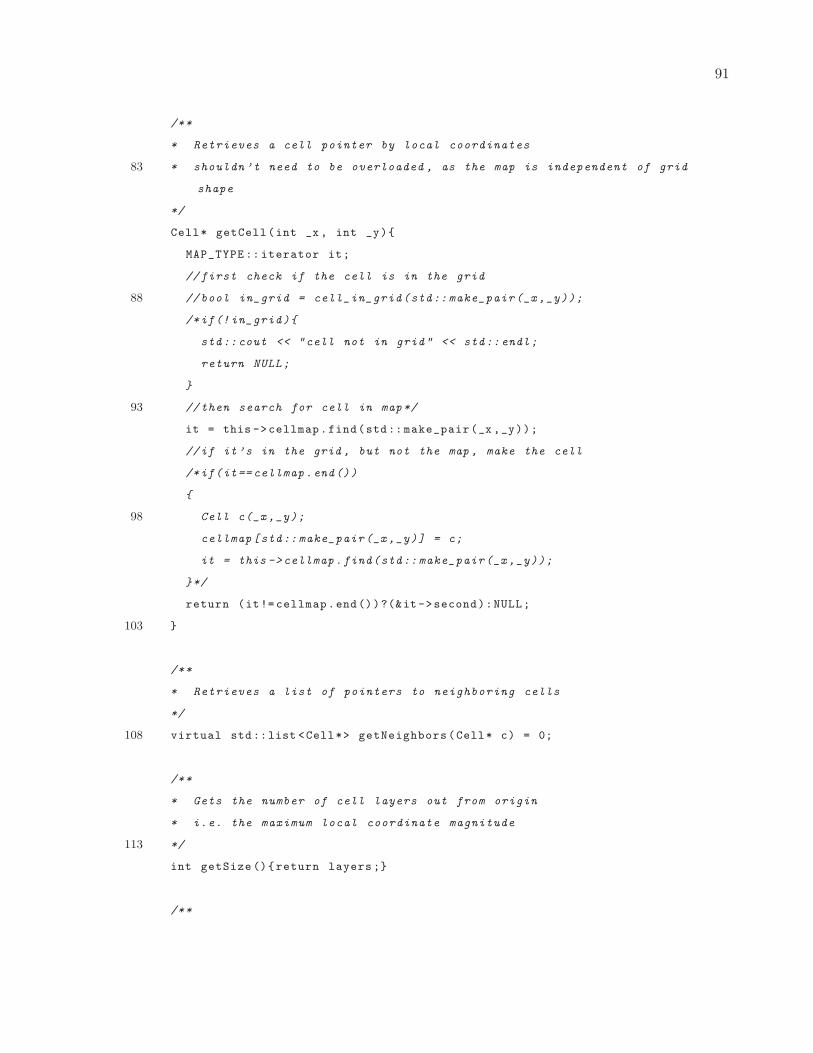
91
/**
* Retrieves a cell pointer by local coordinates
83 * shouldn ’t need to be overloaded , as the map is independent of grid
shape
*/
Cell* getCell(int _x, int _y){
MAP_TYPE :: iterator it;
//first check if the cell is in the grid
88 //bool in_grid = cell_in_grid(std:: make_pair(_x,_y));
/*if(! in_grid){
std::cout << "cell not in grid" << std::endl;
return NULL;
}
93 //then search for cell in map*/
it = this ->cellmap.find(std:: make_pair(_x,_y));
//if it’s in the grid , but not the map , make the cell
/*if(it== cellmap.end())
{
98 Cell c(_x,_y);
cellmap[std:: make_pair(_x ,_y)] = c;
it = this ->cellmap.find(std:: make_pair(_x,_y));
}*/
return (it!= cellmap.end())?(&it->second):NULL;
103 }
/**
* Retrieves a list of pointers to neighboring cells
*/
108 virtual std::list <Cell*> getNeighbors(Cell* c) = 0;
/**
* Gets the number of cell layers out from origin
* i.e. the maximum local coordinate magnitude
113 */
int getSize (){return layers ;}
/**
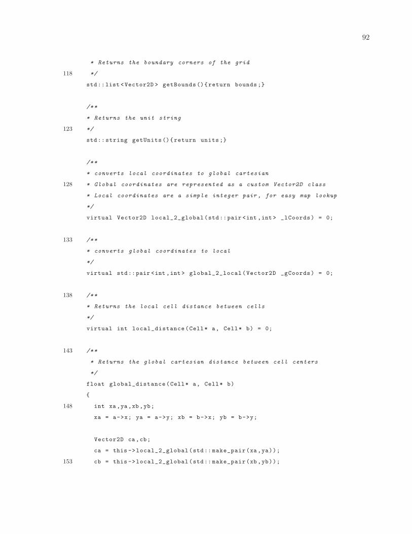
92
* Returns the boundary corners of the grid
118 */
std::list <Vector2D > getBounds (){return bounds ;}
/**
* Returns the unit string
123 */
std:: string getUnits (){return units;}
/**
* converts local coordinates to global cartesian
128 * Global coordinates are represented as a custom Vector2D class
* Local coordinates are a simple integer pair , for easy map lookup
*/
virtual Vector2D local_2_global(std::pair <int ,int > _lCoords) = 0;
133 /**
* converts global coordinates to local
*/
virtual std::pair <int ,int > global_2_local(Vector2D _gCoords) = 0;
138 /**
* Returns the local cell distance between cells
*/
virtual int local_distance(Cell* a, Cell* b) = 0;
143 /**
* Returns the global cartesian distance between cell centers
*/
float global_distance(Cell* a, Cell* b)
{
148 int xa ,ya ,xb ,yb;
xa = a->x; ya = a->y; xb = b->x; yb = b->y;
Vector2D ca,cb;
ca = this ->local_2_global(std:: make_pair(xa,ya));
153 cb = this ->local_2_global(std:: make_pair(xb,yb));
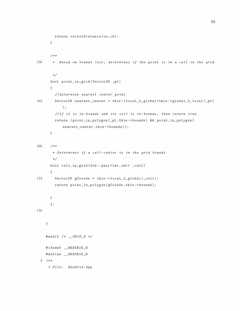
93
return vectorDistance(ca,cb);
}
/**
158 * Based on bounds list , determines if the point is in a cell in the grid
.
*/
bool point_in_grid(Vector2D _pt)
{
// determine nearest center point
163 Vector2D nearest_center = this ->local_2_global(this ->global_2_local(_pt)
);
//if it is in-bounds and its cell is in-bounds , then return true
return (point_in_polygon(_pt ,this ->bounds) && point_in_polygon(
nearest_center ,this ->bounds));
}
168 /**
* Determines if a cell -center is in the grid bounds
*/
bool cell_in_grid(std::pair <int ,int > _cell)
{
173 Vector2D gCoords = this ->local_2_global(_cell);
return point_in_polygon(gCoords ,this ->bounds);
}
};
178
}
#endif /* __GRID_H */
#ifndef __HEXGRID_H
#define __HEXGRID_H
3 /**
* File: HexGrid.hpp
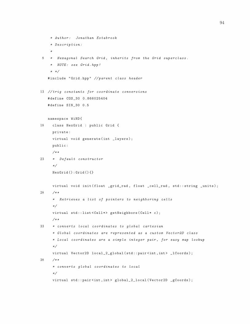
94
* Author: Jonathan Estabrook
* Description:
*
8 * Hexagonal Search Grid , inherits from the Grid superclass.
* NOTE: see Grid.hpp!
* */
#include "Grid.hpp" // parent class header
13 //trig constants for coordinate conversions
#define COS_30 0.866025404
#define SIN_30 0.5
namespace WiND{
18 class HexGrid : public Grid {
private:
virtual void generate(int _layers);
public:
/**
23 * Default constructor
*/
HexGrid ():Grid(){}
virtual void init(float _grid_rad , float _cell_rad , std:: string _units);
28 /**
* Retrieves a list of pointers to neighboring cells
*/
virtual std::list <Cell*> getNeighbors(Cell* c);
/**
33 * converts local coordinates to global cartesian
* Global coordinates are represented as a custom Vector2D class
* Local coordinates are a simple integer pair , for easy map lookup
*/
virtual Vector2D local_2_global(std::pair <int ,int > _lCoords);
38 /**
* converts global coordinates to local
*/
virtual std::pair <int ,int > global_2_local(Vector2D _gCoords);
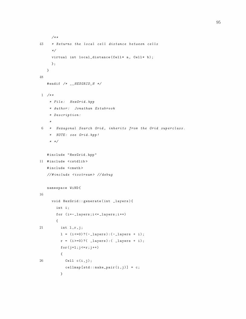
95
/**
43 * Returns the local cell distance between cells
*/
virtual int local_distance(Cell* a, Cell* b);
};
}
48
#endif /* __HEXGRID_H */
1 /**
* File: HexGrid.hpp
* Author: Jonathan Estabrook
* Description:
*
6 * Hexagonal Search Grid , inherits from the Grid superclass.
* NOTE: see Grid.hpp!
* */
#include "HexGrid.hpp"
11 #include <cstdlib >
#include <cmath >
//#include <iostream > //debug
namespace WiND{
16
void HexGrid :: generate(int _layers){
int i;
for (i=-_layers;i<= _layers;i++)
{
21 int l,r,j;
l = (i<=0)?(-_layers):(-_layers + i);
r = (i>=0)?( _layers):( _layers + i);
for(j=l;j<=r;j++)
{
26 Cell c(i,j);
cellmap[std:: make_pair(i,j)] = c;
}
96
}
}
31
/**
* grid generation function based on minor grid radius and minor cell
radius
*/
void HexGrid ::init(float _grid_rad , float _cell_rad , std:: string _units)
36 {
//NOTE: changed to floor to ensure whole -cell layer bounds
this ->layers = std::floor (( _grid_rad/COS_30)/(( _cell_rad)*2)); //
calculate cell layers
this ->scale = (_cell_rad)*2; // scaling factor should be twice the minor
cell radius
this ->units = _units;
41
//fill the boundary list
float R = _grid_rad/COS_30;
// std::cout << this ->layers << " layers , " << this ->scale << " scale , "
<< R << " grid_rad" << std::endl;
46
Vector2D pt;
pt.x = 0; pt.y = R;
this ->bounds.push_back(pt);
pt.x = R*COS_30; pt.y = R*SIN_30;
51 this ->bounds.push_back(pt);
pt.y = -pt.y;
this ->bounds.push_back(pt);
pt.x = 0; pt.y = -R;
this ->bounds.push_back(pt);
56 pt.x = -R*COS_30; pt.y = -R*SIN_30;
this ->bounds.push_back(pt);
pt.y = -pt.y;
this ->bounds.push_back(pt);
97
61 // removing this for now , cells should be created on-demand from boundary
points
this ->generate(layers);
}
// virtual
66 std::list <Cell*> HexGrid :: getNeighbors(Cell* c)
{
std::list <Cell*> cells;
// calculate neighbor coordinates
//first the upper neighbor , go clockwise from here
71 int x,y; x = c->x; y = c->y;
Cell* neighbor;
// N (0,+)
neighbor = getCell(x ,y+1);
if(neighbor) cells.push_back(neighbor);
76 // NE (+,+)
neighbor = getCell(x+1,y+1);
if(neighbor) cells.push_back(neighbor);
// SE (+,0)
neighbor = getCell(x+1,y );
81 if(neighbor) cells.push_back(neighbor);
// S (0,-)
neighbor = getCell(x ,y-1);
if(neighbor) cells.push_back(neighbor);
// SW (-,-)
86 neighbor = getCell(x-1,y-1);
if(neighbor) cells.push_back(neighbor);
// NW (-,0)
neighbor = getCell(x-1,y );
if(neighbor) cells.push_back(neighbor);
91
return cells;
}
/**
96 * converts local coordinates to global cartesian
98
* Global coordinates are represented as a custom Vector2D class
* Local coordinates are a simple integer pair , for easy map lookup
*/
Vector2D HexGrid :: local_2_global(std::pair <int ,int > _lCoords)
101 {
int lx = _lCoords.first;
int ly = _lCoords.second;
Vector2D gCoords;
gCoords.x = (( float)lx*COS_30)*this ->scale;
106 gCoords.y = (( float)ly - (float)lx*SIN_30)*this ->scale;
return gCoords;
}
/**
* converts global coordinates to local
111 */
std::pair <int ,int > HexGrid :: global_2_local(Vector2D _gCoords)
{
float gx = _gCoords.x;
float gy = _gCoords.y;
116 int lx = floor(gx/( COS_30*this ->scale) + 0.5);
int ly = floor(gy/scale+lx*SIN_30 + 0.5);
return std:: make_pair(lx,ly);
}
121 /**
* Returns the local cell distance between cells
*/
int HexGrid :: local_distance(Cell* a, Cell* b)
{
126 int x1 ,y1 ,x2 ,y2;
x1 = a->x; y1 = a->y; x2 = b->x; y2 = b->y;
int A = std::abs(x2 - x1);
int B = std::abs(y2 - y1);
131 int C = std::abs(a - b);
return (C>(A>B?A:B))?C:(A>B?A:B); //max of 3 for hexagonal coordinates
}
99
}
1 #ifndef __SEARCHALGS_H
#define __SEARCHALGS_H
/**
* File: WiND_search.hpp
* Author: Jonathan Estabrook
6 * Description:
*
* Function Library for search methods.
* */
11 #include "Grid.hpp"
#include "WiND_utils.hpp"
#include <set >
#include <list >
16
namespace WiND
{
/**
* computes next cell for a spiral about origin (0,0)
21 **/
Cell* getNextSpiral(Cell* _current , Grid* _grid);
std::list <Cell*> planPath(Cell* _current , Cell* _target , Grid* _grid);
26 /**
* Returns the nearest unvisited cell ,
* breaks ties by returning the one with the highest probability.
**/
Cell* getNextUnvisited(Cell* _current , Grid* _grid);
31
/**
* Returns the nearest allowed cell , regardless of being visited or
probability
**/
100
Cell* getNearestAllowed(Cell* _current , Grid* _grid);
36
/**
* Determines if a cell is in a specified triangle
**/
bool isCellInTriangle(Vector2D a, Vector2D b, Vector2D c, Cell* _cell ,
Grid* _grid);
41
/**
* Returns a list of cells in a specified triangle
**/
std::set <Cell*> getCellsInTriangle( Vector2D a, Vector2D b, Vector2D c,
Grid* _grid);
46 }
#endif /* SEARCHALGS_H */
/**
* File: WiND_search.cpp
3 * Author: Jonathan Estabrook
* Description:
*
* Function Library for search methods.
* */
8 #include "WiND_search.hpp"
#include "WiND_utils.hpp"
#include <algorithm >
#include <list >
13 #include <set >
#include <map >
namespace WiND {
18 /**
* Data struct for path planning , currently specialized for A* search
*/
struct SearchNode{
101
Cell* cell;
23 SearchNode* parent;
unsigned int G; //cost to this cell
unsigned int H; // estimated cost(straight line)
SearchNode(Cell* _c , SearchNode* _p , unsigned int _G , unsigned int _H)
28 :cell(_c),parent(_p),G(_G),H(_H){}
};
/*
* Spiral/sweep navigation , should work on square grids too when
implemented
33 */
Cell* getNextSpiral(Cell* _current , Grid* _grid)
{
std::list <Cell*> neighbors = _grid ->getNeighbors(_current);
std::list <Cell*>:: iterator it;
38
Cell* next = NULL; // initialize to null for failure check
float odist ,min;
min = -1;
43
Cell* origin = _grid ->getCell (0,0);
for(it = neighbors.begin(); it!= neighbors.end(); it++)
{
48 if( !(*it)->visited && (*it)->allowed ){
odist = _grid ->global_distance(origin ,*it);
if(odist <= min || (min < 0)){next=*it; min=odist ;}
}
}
53
return next;
}
102
58 /**
* Cell -list path planning
*/
std::list <Cell*> planPath(Cell* _current , Cell* _target , Grid* _grid)
{
63 std::list <SearchNode > store; //store nodes in memory so we can have
valid pointers
std::list <Cell*>:: iterator cit;
std::list <Cell*> path; // return path
std::map < Cell*, SearchNode* >::iterator it;
std::map < Cell*, SearchNode* > open; //open map
68 std::map < Cell*, SearchNode* > closed; // closed map
SearchNode start(_current ,NULL ,0.0,_grid ->global_distance(_current ,
_target));
store.push_back(start); //store node
open[_current] = &(store.back()); //place start cell in open list
73
SearchNode* current_node = &( store.back());
// get the first cell , starting at origin for now
// TODO: make this a bit more efficient
while(!open.empty() && (current_node ->cell != _target)){
78 //drop current node from open set , place in closed set
closed[current_node ->cell] = current_node;
open.erase(current_node ->cell);
std::list <Cell*> neighbors = _grid ->getNeighbors(current_node ->cell);
// process neighbors
83 for(cit = neighbors.begin(); cit != neighbors.end(); cit ++)
{
bool inClosed = (closed.find(*cit) != closed.end());
bool isAllowed = (*cit)->allowed;
bool inOpen = (open.find(*cit) != open.end());
88
if(! inClosed && !inOpen && isAllowed){ //if not visited and allowed
SearchNode node(
*cit ,
current_node ,
103
93 current_node ->G + _grid ->local_distance(current_node ->cell ,*cit)
,
_grid ->local_distance (*cit ,_target));
store.push_back(node);
open[*cit] = &(store.back()); //place in open set
} else if(inOpen){// check if path is more optimal
98 SearchNode* node = open[*cit];
unsigned int G = current_node ->G + _grid ->local_distance(
current_node ->cell ,*cit);
unsigned int cG = node ->G;
if(G < cG){ //if the path is more optimal
node ->parent = current_node; // update parent
103 node ->G = G; // update G-score (H should be same in this case)
}
}
}
//find the lowest cost node in the open list
108 float F = -1;
for(it = open.begin(); it != open.end(); it++)
{
SearchNode* node = it->second;
float cF = node ->G + node ->H;
113 if(F == -1 || cF < F){
current_node = node; //set next node
F = cF; // update cost
}
}
118 }
if(current_node ->cell == _target){
SearchNode* traceback = current_node;
while(traceback ->parent){ // while the next parent is not null
path.push_front(traceback ->cell); //add cell to path
123 traceback = traceback ->parent; //visit parent
}
}
return path;
104
128 }
/**
* Returns the nearest unvisited cell
*/
133
Cell* getNextUnvisited(Cell* _current , Grid* _grid)
{
std::list <Cell*> neighbors;
std::list <Cell*> fringe;
138 std::set <Cell*> explored;
std::list <Cell*>:: iterator it;
Cell* next = NULL;
143 fringe.push_back(_current);
while(! fringe.empty())
{
if(fringe.front()->visited)
{
148 neighbors = _grid ->getNeighbors(fringe.front());
// explored.insert(fringe.front ());
fringe.pop_front ();
for(it = neighbors.begin(); it != neighbors.end(); it++)
{
153 if(explored.find(*it) == explored.end() && (*it)->allowed)
{
fringe.push_back (*it);
explored.insert (*it);
}
158 }
}
else
{
float max = 0;
163 for(it = fringe.begin(); it != fringe.end(); it++)
{
105
float P = (*it)->probability;
if(P > max)
{
168 next = *it;
max = P;
}
}
break;
173 }
}
return next;
}
178
/**
* Returns the nearest allowed cell
* Useful for handling unexpected blocked conditions
*/
183
Cell* getNearestAllowed(Cell* _current , Grid* _grid)
{
std::list <Cell*> neighbors;
std::list <Cell*> fringe;
188 std::set <Cell*> explored;
std::list <Cell*>:: iterator it;
Cell* next = NULL; // pointer to the next cell , initialized to null
193 fringe.push_back(_current);
while(! fringe.empty()) // while fringe isn’t empty and no next cell is
assigned
{
if(!( fringe.front ()->allowed)) //if the cell isn’t open , expand out
{
198 neighbors = _grid ->getNeighbors(fringe.front());
fringe.pop_front ();
for(it = neighbors.begin(); it != neighbors.end(); it++)
106
{
if(explored.find(*it) == explored.end()) //if unexplored
203 {
fringe.push_back (*it);
explored.insert (*it);
}
}
208 }
else //if the fringe front is allowed , we’ve found at least one open
cell
{
float min = -1;
for(it = fringe.begin(); it != fringe.end(); it++)
213 {
float D = _grid ->global_distance (*it ,_current);
if(min == -1 || D < min)
{
next = *it;
218 min = D;
}
}
break;
}
223 }
return next;
}
bool isCellInTriangle(Vector2D a, Vector2D b, Vector2D c, Cell* _cell ,
Grid* _grid)
228 {
int x,y; x = _cell ->x; y = _cell ->y;
//round the points to nearest cell center coordinates
Vector2D A = _grid ->local_2_global(_grid ->global_2_local(a));
Vector2D B = _grid ->local_2_global(_grid ->global_2_local(b));
233 Vector2D C = _grid ->local_2_global(_grid ->global_2_local(c));
Vector2D pt = _grid ->local_2_global(std:: make_pair(x,y));
107
return isInTriangle(A,B,C,pt); //call to geometry function
// return isInTriangle(a,b,c,pt);
238 }
std::set <Cell*> getCellsInTriangle(Vector2D a, Vector2D b, Vector2D c,
Grid* _grid)
{
std::set <Cell*> cells;
243 std::list <Cell*> neighbors;
std::set <Cell*> explored;
std::list <Cell*> fringe;
std::list <Cell*>:: iterator it;
// get the first cell , starting at origin for now
248 // TODO: this could probably be made a bit more efficient
Cell* cell = _grid ->getCell (0,0);
fringe.push_back(cell);
explored.insert(cell);
while(! fringe.empty())
253 {
neighbors = _grid ->getNeighbors(fringe.front());
// explored.insert(fringe.front ());
// check if current cell is in triangle
258 if(isCellInTriangle(a,b,c,fringe.front (),_grid))
{
cells.insert(fringe.front());
}
//pop from fringe
263 fringe.pop_front ();
//add neighbors
for(it = neighbors.begin(); it != neighbors.end(); it++)
{
if(explored.find(*it)== explored.end())
268 {
fringe.push_back (*it);
explored.insert (*it);
}
108
}
273 }
return cells;
}
}
#ifndef __WIND_GEOMETRY_H
#define __WIND_GEOMETRY_H
3 /**
* File: WiND_utils.hpp
* Author: Jonathan Estabrook
* Description:
*
8 * Basic utility functions and useful data type library.
* Geometric functions and such should go here for usage in other places.
* */
#include <list >
namespace WiND
13 {
/**
* Waypoint Data Struct ,
* Relative to 0,0,0 cartesian on grid
*/
18 struct Waypoint{
float x;
float y;
float z;
};
23
struct Vector2D{
/** The coordinates
******************* */
float x;
28 float y;
/** Operators
******************* */
109
Vector2D add(const Vector2D &v)
{Vector2D p = {x+v.x,y+v.y}; return p;}
33
Vector2D sub(const Vector2D &v)
{Vector2D p = {x-v.x,y-v.y}; return p;}
float dot(const Vector2D &v)
38 {return (x*v.x+y*v.y);}
//don’t need cross product for now
};
43 /**** GEOMETRY FUNCTIONS ****/
bool isInTriangle(Vector2D a, Vector2D b, Vector2D c, Vector2D target);
float vectorDistance(Vector2D a, Vector2D b);
48 bool point_in_polygon(Vector2D _pt , std::list <Vector2D > _polygon);
}
#endif
/**
* File: WiND_geometry.cpp
* Author: Jonathan Estabrook
* Description: basic geometric functions
5 */
#include "WiND_utils.hpp"
#include <cmath >
10 namespace WiND
{
/**
* Returns if target is in triangle defined by a,b,c
*/
15 bool isInTriangle(Vector2D a, Vector2D b, Vector2D c, Vector2D target){
// Compute edges
110
Vector2D v0 = c.sub(a);
Vector2D v1 = b.sub(a);
Vector2D v2 = target.sub(a);
20
// Compute dot products
float dot00 = v0.dot(v0);
float dot01 = v0.dot(v1);
float dot02 = v0.dot(v2);
25 float dot11 = v1.dot(v1);
float dot12 = v1.dot(v2);
// Compute barycentric coordinates
float invDenom = 1/( dot00 * dot11 - dot01 * dot01);
30 float u = (dot11 * dot02 - dot01 * dot12) * invDenom;
float v = (dot00 * dot12 - dot01 * dot02) * invDenom;
// Check if point is in triangle
return (u >= 0) && (v >= 0) && (u + v < 1);
35 }
/**
* Returns vector distance between points
*/
float vectorDistance(Vector2D a, Vector2D b)
40 {
return std::sqrt((b.x-a.x)*(b.x-a.x)+(b.y-a.y)*(b.y-a.y));
}
bool point_in_polygon(Vector2D _pt , std::list <Vector2D > _polygon)
45 {
std::list <Vector2D >:: iterator it ,last;
it = _polygon.begin (); last = it; it++;
bool oddCrosses = false;
for(; it != _polygon.end(); it++)
50 {
float ix,jx,iy ,jy;
ix = (*it).x; iy = (*it).y; jx = (*last).x; jy = (*last).y;
if(( (jy < _pt.y && iy >= _pt.y) ||
111
(iy < _pt.y && jy >= _pt.y)) &&
55 (ix <= _pt.x && jx <= _pt.x))
{
if(ix + (_pt.y-iy)/(jy-iy)*(jx-ix)< _pt.x)
{
oddCrosses = !oddCrosses;
60 }
last = it;
}
}
return oddCrosses;
65
}
}
/**
2 * File: test.cpp
* Simple demo file for hexagonal grid navigation
*/
#include <iostream > //for debug
#include <list >
7 #include <utility >
#include "Grid.hpp"
#include "Agent.hpp"
#include "WiND_search.hpp"
#include "WiND_utils.hpp"
12
/**
* Usage specific , prints grid to prompt
*/
void print_grid(WiND::Agent& a)
17 {
int size = a.getWorld ()->getSize ();
for(int i=size; i >= -size; i--)
{
std:: string p;
112
22 if(i<0){
p.assign(-i,’ ’);
std::cout << p;
}
for(int j=-size; j <= size; j++)
27 {
WiND::Cell* s = a.getWorld ()->getCell(j,i);
if(s){
if(s == a.getCurrentCell ()) std::cout << "X ";
32 else if(s->visited) std::cout << "o ";
else if(!s->allowed) std::cout << "- ";
else std::cout << ". ";
}
else std::cout << " ";
37 }
std::cout << std::endl;
}
}
42 void callback_test(const char* _event , const char* _arg)
{
std::cout << "CALLBACK: " << _event << ":" << _arg << std::endl;
}
47 /**
* Main function
*/
int main()
{
52
WiND::Agent agent (50.0 ,3.0 ,"meters","hexagon"); // should make a roughly
12-layer grid
agent.setPosition ( -10.0 ,3.0 ,100.0);
// agent.setPosition (5 ,5,100);
agent.setTargetAltitude (300);
57 // agent.setTargetPoint (30 ,30);
113
agent.setCallback(callback_test);
WiND:: Vector2D a = {0 ,0};
WiND:: Vector2D b = {-25,-0.1};
62 WiND:: Vector2D c = {0 ,25};
WiND::Grid* grid = agent.getWorld ();
67 std::set <WiND::Cell*> triangle = WiND:: getCellsInTriangle(a,b,c,grid);
std::set <WiND::Cell*>:: iterator it;
for(it = triangle.begin(); it != triangle.end(); it++) {(*it)->allowed =
false ;}
std::cout << "Testing Agent Navigation , non -center starting position" <<
std::endl;
72 std::cin.ignore ();
print_grid(agent);
WiND:: Waypoint next;
WiND:: Waypoint pos;
77
while(true)
{
next = agent.getNextWaypoint ();
pos = agent.getPosition ();
82 WiND:: Vector2D gCoords = {pos.x,pos.y};
std::pair <int ,int > hpos = agent.getWorld ()->global_2_local(gCoords);
if(next.x == pos.x && next.y == pos.y) break;
std::cout << pos.x << "," << pos.y << "," << pos.z << std::endl;
std::cout << hpos.first << "," << hpos.second << std::endl;
87 print_grid(agent); // print current state
agent.setPosition(next.x, next.y, next.z); // update position
usleep (200000);
}
print_grid(agent);
92 std::cout << "done ..." << std::endl;

114
}
115
Appendix D
Framework Outline
2 module.exports = require(’./lib/WiND’);
/**
2 * File: WiND.cc
* Author: Jonathan Estabrook
* Description:
*
* This file is the binding between the libWiND library and its NodeJS
module.
7 * Bindings between C/C++ and Javascript happen here.
*
* For any methods/function bindings , add a wrapper method within the
WiND_node
* class here. Other utility methods can be added directly here too , and
bound to
* the Javascript module.
12 **/
#include <v8.h>
#include <node.h>
#include <string >
17 #include <sstream >
#include <list >
116
// the WiND library
#include <WiND/Agent.hpp >
22
using namespace v8;
using namespace node;
//some useful macros for repetitive v8 conversion tasks
27 // see http :// github.com/pquerna/node -extension -examples
#define REQ_STR_ARG(I, VAR) \
if(args.Length () <= I || !args[I]->IsString ()) \
return ThrowException(Exception :: TypeError( \
String ::New("Argument " #I " must be a string"))); \
32 Local <String > VAR = Local <String >:: Cast(args[I])
#define REQ_FUN_ARG(I, VAR) \
if(args.Length () <= I || !args[I]->IsFunction ()) \
return ThrowException(Exception :: TypeError( \
37 String ::New("Argument " #I " must be a function"))); \
Local <Function > VAR = Local <Function >:: Cast(args[I])
#define REQ_FLO_ARG(I, VAR) \
if(args.Length () <= I || !args[I]->IsNumber ()) \
42 return ThrowException(Exception :: TypeError( \
String ::New("Argument " #I " must be a number"))); \
Local <Number > VAR = Local <Number >:: Cast(args[I])
#define TO_STRING(V8STR ,ASCIISTR ,VAR) \
47 String :: AsciiValue ASCIISTR(V8STR); \
const char* VAR = *ASCIISTR
#define TO_V8STRING(STR ,VAR) \
Local <String > VAR = String ::New(STR)
52
#define CHECK_POINTER(PTR ,ERRMSG) \
if(!PTR) return ThrowException(Exception :: ReferenceError(String ::New(
ERRMSG)))
117
57 namespace WiND_node{
class Agent : ObjectWrap
{
private:
WiND:: Agent* m_agent; // pointer to wrapped WiND::Agent
62 public:
static Persistent <FunctionTemplate > s_ct;
static void Init(Handle <Object > target)
{
HandleScope scope;
67 Local <FunctionTemplate > t = FunctionTemplate ::New(New);
s_ct = Persistent <FunctionTemplate >:: New(t);
s_ct ->InstanceTemplate ()->SetInternalFieldCount (1);
s_ct ->SetClassName(String :: NewSymbol("Agent"));
72
//to bind c++ methods to the javascript follow this template:
// NODE_SET_PROTOTYPE_METHOD(s_ct , "js_name", cpp_name);
NODE_SET_PROTOTYPE_METHOD(s_ct , "configure", Configure);
NODE_SET_PROTOTYPE_METHOD(s_ct , "deconfigure", Deconfigure);
77 NODE_SET_PROTOTYPE_METHOD(s_ct , "get_position", GetPosition);
NODE_SET_PROTOTYPE_METHOD(s_ct , "set_position", SetPosition);
NODE_SET_PROTOTYPE_METHOD(s_ct , "get_next_waypoint", GetNextWaypoint);
NODE_SET_PROTOTYPE_METHOD(s_ct , "get_grid_bounds", GetGridBounds);
NODE_SET_PROTOTYPE_METHOD(s_ct , "set_target_point", SetTargetPoint);
82 NODE_SET_PROTOTYPE_METHOD(s_ct , "set_target_altitude",
SetTargetAltitude);
target ->Set(String :: NewSymbol("Agent"),s_ct ->GetFunction ());
}
87 Agent():m_agent(NULL){} // constructor
~Agent()
{
delete this ->m_agent;
118
this ->m_agent = NULL;
92 }
// v8 method for constructing from Javascript
static Handle <Value > New(const Arguments& args)
{
97 HandleScope scope;
Agent* hw = new Agent(); // create a WiND_node ::Agent object
hw ->Wrap(args.This()); // store refernece inside args.This();
return args.This(); // return reference from args.This();
}
102
// configure wrapper method , sends initialization request to Agent
static Handle <Value > Configure(const Arguments& args)
{
HandleScope scope;
107 Agent* a = ObjectWrap ::Unwrap <Agent >(args.This());
if(a->m_agent) return ThrowException(Exception :: ReferenceError(
String ::New("Agent already initialized , use deconfigure first")));
REQ_FLO_ARG (0, _min_grid_rad);
REQ_FLO_ARG (1, _min_cell_rad);
112 REQ_STR_ARG (2,_units);
REQ_STR_ARG (3, _grid_type);
float mgr = _min_grid_rad ->Value();
float mcr = _min_cell_rad ->Value();
117 TO_STRING(_units ,unitval ,u);
TO_STRING(_grid_type ,gtval ,gt);
a->m_agent = new WiND::Agent(mgr ,mcr ,u,gt);
return scope.Close(Null());
122 }
// deconfigure method , simply deletes the agent for a hard -reset
// could be made a bit better in the future if needed
static Handle <Value > Deconfigure(const Arguments& args)
127 {
119
HandleScope scope;
Agent* a = ObjectWrap ::Unwrap <Agent >(args.This());
if(a->m_agent){
delete a->m_agent;
132 a->m_agent = NULL;
}
return scope.Close(Null());
}
137 static Handle <Value > GetPosition(const Arguments& args)
{
HandleScope scope;
Agent* a = ObjectWrap ::Unwrap <Agent >(args.This());
CHECK_POINTER(a->m_agent ,"Agent is not initialized!");
142 WiND:: Waypoint wp = a->m_agent ->getPosition ();
std:: stringstream ss;
ss << "{\" TYPE \":\" WAYPOINT \"";
ss << " ,\"UNIT \":\"" << a->m_agent ->getWorld ()->getUnits () << "\"";
ss << " ,\"X\":" << wp.x;
147 ss << " ,\"Y\":" << wp.y;
ss << " ,\"Z\":" << wp.z << "}";
TO_V8STRING(ss.str().c_str (),result);
return scope.Close(result);
}
152
static Handle <Value > SetPosition(const Arguments& args)
{
HandleScope scope;
Agent* a = ObjectWrap ::Unwrap <Agent >(args.This());
157 CHECK_POINTER(a->m_agent ,"Agent is not initialized!");
REQ_FLO_ARG (0,_x);
REQ_FLO_ARG (1,_y);
REQ_FLO_ARG (2,_z);
float x = _x->Value();
162 float y = _y->Value();
float z = _z->Value();
a->m_agent ->setPosition(x,y,z);
120
return scope.Close(Null());
}
167
static Handle <Value > GetNextWaypoint(const Arguments& args)
{
HandleScope scope;
Agent* a = ObjectWrap ::Unwrap <Agent >(args.This());
172 CHECK_POINTER(a->m_agent ,"Agent is not initialized!");
WiND:: Waypoint wp = a->m_agent ->getNextWaypoint ();
std:: stringstream ss;
ss << "{\" TYPE \":\" WAYPOINT \"";
ss << " ,\"UNIT \":\"" << a->m_agent ->getWorld ()->getUnits () << "\"";
177 ss << " ,\"X\":" << wp.x;
ss << " ,\"Y\":" << wp.y;
ss << " ,\"Z\":" << wp.z << "}";
TO_V8STRING(ss.str().c_str (),result);
return scope.Close(result);
182 }
static Handle <Value > GetGridBounds(const Arguments& args)
{
HandleScope scope;
187 Agent* a = ObjectWrap ::Unwrap <Agent >(args.This());
CHECK_POINTER(a->m_agent ,"Agent is not initialized!");
std::list <WiND::Vector2D > bounds = a->m_agent ->getWorld ()->getBounds ()
;
std::list <WiND::Vector2D >:: iterator it;
std:: stringstream ss;
192 ss << "[";
for(it=bounds.begin();it!= bounds.end();it++)
{
if(it!= bounds.begin ()) ss << ",";
ss << "{\"x\":" << (*it).x << " ,\"y\":" << (*it).y << "}";
197 }
ss << "]";
TO_V8STRING(ss.str().c_str (),result);
return scope.Close(result);
121
}
202
static Handle <Value > SetTargetPoint(const Arguments& args)
{
HandleScope scope;
Agent* a = ObjectWrap ::Unwrap <Agent >(args.This());
207 CHECK_POINTER(a->m_agent ,"Agent is not initialized!");
REQ_FLO_ARG (0, _x);
REQ_FLO_ARG (1, _y);
float x = _x->Value();
float y = _y->Value();
212 a->m_agent ->setTargetPoint(x,y);
return scope.Close(Null());
}
static Handle <Value > SetTargetAltitude(const Arguments& args)
217 {
HandleScope scope;
Agent* a = ObjectWrap ::Unwrap <Agent >(args.This());
CHECK_POINTER(a->m_agent ,"Agent is not initialized!");
REQ_FLO_ARG (0, _z);
222 float z = _z->Value();
a->m_agent ->setTargetAltitude(z);
return scope.Close(Null());
}
227 };
/* **********************************************
* The code below is needed for bindings to work properly
* Bindings to other objects would need to place their Init() methods
232 * within the init function below.
**/
Persistent <FunctionTemplate > Agent::s_ct;
extern "C" {
237 static void init (Handle <Object > target)
122
{
Agent ::Init(target);
}
242 NODE_MODULE(WiND , init);
}
}
/**
* File: WiND.cc
* Author: Jonathan Estabrook
4 * Description:
*
* This file is the binding between the libWiND library and its NodeJS
module.
* Bindings between C/C++ and Javascript happen here.
*
9 * For any methods/function bindings , add a wrapper method within the
WiND_node
* class here. Other utility methods can be added directly here too , and
bound to
* the Javascript module.
**/
14 #include <v8.h>
#include <node.h>
#include <string >
#include <sstream >
#include <list >
19
// the WiND library
#include <WiND/Agent.hpp >
using namespace v8;
24 using namespace node;
123
//some useful macros for repetitive v8 conversion tasks
// see http :// github.com/pquerna/node -extension -examples
#define REQ_STR_ARG(I, VAR) \
29 if(args.Length () <= I || !args[I]->IsString ()) \
return ThrowException(Exception :: TypeError( \
String ::New("Argument " #I " must be a string"))); \
Local <String > VAR = Local <String >:: Cast(args[I])
34 #define REQ_FUN_ARG(I, VAR) \
if(args.Length () <= I || !args[I]->IsFunction ()) \
return ThrowException(Exception :: TypeError( \
String ::New("Argument " #I " must be a function"))); \
Local <Function > VAR = Local <Function >:: Cast(args[I])
39
#define REQ_FLO_ARG(I, VAR) \
if(args.Length () <= I || !args[I]->IsNumber ()) \
return ThrowException(Exception :: TypeError( \
String ::New("Argument " #I " must be a number"))); \
44 Local <Number > VAR = Local <Number >:: Cast(args[I])
#define TO_STRING(V8STR ,ASCIISTR ,VAR) \
String :: AsciiValue ASCIISTR(V8STR); \
const char* VAR = *ASCIISTR
49
#define TO_V8STRING(STR ,VAR) \
Local <String > VAR = String ::New(STR)
#define CHECK_POINTER(PTR ,ERRMSG) \
54 if(!PTR) return ThrowException(Exception :: ReferenceError(String ::New(
ERRMSG)))
namespace WiND_node{
class Agent : ObjectWrap
59 {
private:
WiND:: Agent* m_agent; // pointer to wrapped WiND::Agent
124
public:
static Persistent <FunctionTemplate > s_ct;
64 static void Init(Handle <Object > target)
{
HandleScope scope;
Local <FunctionTemplate > t = FunctionTemplate ::New(New);
69 s_ct = Persistent <FunctionTemplate >:: New(t);
s_ct ->InstanceTemplate ()->SetInternalFieldCount (1);
s_ct ->SetClassName(String :: NewSymbol("Agent"));
//to bind c++ methods to the javascript follow this template:
74 // NODE_SET_PROTOTYPE_METHOD(s_ct , "js_name", cpp_name);
NODE_SET_PROTOTYPE_METHOD(s_ct , "configure", Configure);
NODE_SET_PROTOTYPE_METHOD(s_ct , "deconfigure", Deconfigure);
NODE_SET_PROTOTYPE_METHOD(s_ct , "get_position", GetPosition);
NODE_SET_PROTOTYPE_METHOD(s_ct , "set_position", SetPosition);
79 NODE_SET_PROTOTYPE_METHOD(s_ct , "get_next_waypoint", GetNextWaypoint);
NODE_SET_PROTOTYPE_METHOD(s_ct , "get_grid_bounds", GetGridBounds);
NODE_SET_PROTOTYPE_METHOD(s_ct , "set_target_point", SetTargetPoint);
NODE_SET_PROTOTYPE_METHOD(s_ct , "set_target_altitude",
SetTargetAltitude);
84 target ->Set(String :: NewSymbol("Agent"),s_ct ->GetFunction ());
}
Agent():m_agent(NULL){} // constructor
~Agent()
89 {
delete this ->m_agent;
this ->m_agent = NULL;
}
94 // v8 method for constructing from Javascript
static Handle <Value > New(const Arguments& args)
{
HandleScope scope;
125
Agent* hw = new Agent(); // create a WiND_node ::Agent object
99 hw ->Wrap(args.This()); // store refernece inside args.This();
return args.This(); // return reference from args.This();
}
// configure wrapper method , sends initialization request to Agent
104 static Handle <Value > Configure(const Arguments& args)
{
HandleScope scope;
Agent* a = ObjectWrap ::Unwrap <Agent >(args.This());
if(a->m_agent) return ThrowException(Exception :: ReferenceError(
109 String ::New("Agent already initialized , use deconfigure first")));
REQ_FLO_ARG (0, _min_grid_rad);
REQ_FLO_ARG (1, _min_cell_rad);
REQ_STR_ARG (2,_units);
REQ_STR_ARG (3, _grid_type);
114
float mgr = _min_grid_rad ->Value();
float mcr = _min_cell_rad ->Value();
TO_STRING(_units ,unitval ,u);
TO_STRING(_grid_type ,gtval ,gt);
119
a->m_agent = new WiND::Agent(mgr ,mcr ,u,gt);
return scope.Close(Null());
}
124 // deconfigure method , simply deletes the agent for a hard -reset
// could be made a bit better in the future if needed
static Handle <Value > Deconfigure(const Arguments& args)
{
HandleScope scope;
129 Agent* a = ObjectWrap ::Unwrap <Agent >(args.This());
if(a->m_agent){
delete a->m_agent;
a->m_agent = NULL;
}
134 return scope.Close(Null());
126
}
static Handle <Value > GetPosition(const Arguments& args)
{
139 HandleScope scope;
Agent* a = ObjectWrap ::Unwrap <Agent >(args.This());
CHECK_POINTER(a->m_agent ,"Agent is not initialized!");
WiND:: Waypoint wp = a->m_agent ->getPosition ();
std:: stringstream ss;
144 ss << "{\" TYPE \":\" WAYPOINT \"";
ss << " ,\"UNIT \":\"" << a->m_agent ->getWorld ()->getUnits () << "\"";
ss << " ,\"X\":" << wp.x;
ss << " ,\"Y\":" << wp.y;
ss << " ,\"Z\":" << wp.z << "}";
149 TO_V8STRING(ss.str().c_str (),result);
return scope.Close(result);
}
static Handle <Value > SetPosition(const Arguments& args)
154 {
HandleScope scope;
Agent* a = ObjectWrap ::Unwrap <Agent >(args.This());
CHECK_POINTER(a->m_agent ,"Agent is not initialized!");
REQ_FLO_ARG (0,_x);
159 REQ_FLO_ARG (1,_y);
REQ_FLO_ARG (2,_z);
float x = _x->Value();
float y = _y->Value();
float z = _z->Value();
164 a->m_agent ->setPosition(x,y,z);
return scope.Close(Null());
}
static Handle <Value > GetNextWaypoint(const Arguments& args)
169 {
HandleScope scope;
Agent* a = ObjectWrap ::Unwrap <Agent >(args.This());
127
CHECK_POINTER(a->m_agent ,"Agent is not initialized!");
WiND:: Waypoint wp = a->m_agent ->getNextWaypoint ();
174 std:: stringstream ss;
ss << "{\" TYPE \":\" WAYPOINT \"";
ss << " ,\"UNIT \":\"" << a->m_agent ->getWorld ()->getUnits () << "\"";
ss << " ,\"X\":" << wp.x;
ss << " ,\"Y\":" << wp.y;
179 ss << " ,\"Z\":" << wp.z << "}";
TO_V8STRING(ss.str().c_str (),result);
return scope.Close(result);
}
184 static Handle <Value > GetGridBounds(const Arguments& args)
{
HandleScope scope;
Agent* a = ObjectWrap ::Unwrap <Agent >(args.This());
CHECK_POINTER(a->m_agent ,"Agent is not initialized!");
189 std::list <WiND::Vector2D > bounds = a->m_agent ->getWorld ()->getBounds ()
;
std::list <WiND::Vector2D >:: iterator it;
std:: stringstream ss;
ss << "[";
for(it=bounds.begin();it!= bounds.end();it++)
194 {
if(it!= bounds.begin ()) ss << ",";
ss << "{\"x\":" << (*it).x << " ,\"y\":" << (*it).y << "}";
}
ss << "]";
199 TO_V8STRING(ss.str().c_str (),result);
return scope.Close(result);
}
static Handle <Value > SetTargetPoint(const Arguments& args)
204 {
HandleScope scope;
Agent* a = ObjectWrap ::Unwrap <Agent >(args.This());
CHECK_POINTER(a->m_agent ,"Agent is not initialized!");
128
REQ_FLO_ARG (0, _x);
209 REQ_FLO_ARG (1, _y);
float x = _x->Value();
float y = _y->Value();
a->m_agent ->setTargetPoint(x,y);
return scope.Close(Null());
214 }
static Handle <Value > SetTargetAltitude(const Arguments& args)
{
HandleScope scope;
219 Agent* a = ObjectWrap ::Unwrap <Agent >(args.This());
CHECK_POINTER(a->m_agent ,"Agent is not initialized!");
REQ_FLO_ARG (0, _z);
float z = _z->Value();
a->m_agent ->setTargetAltitude(z);
224 return scope.Close(Null());
}
};
229 /* **********************************************
* The code below is needed for bindings to work properly
* Bindings to other objects would need to place their Init() methods
* within the init function below.
**/
234 Persistent <FunctionTemplate > Agent::s_ct;
extern "C" {
static void init (Handle <Object > target)
{
239 Agent ::Init(target);
}
NODE_MODULE(WiND , init);
}
244
129
}
// A javascript layer to simplify using the binding
var WiND = require(’../ build/Release/WiND.node’);
4 var Tester = require(’./ Tester ’);
module.exports.Agent = WiND.Agent;
module.exports.Tester = Tester;
// a simple means of testing navigation by providing smooth movement
feedback
3 var util = require(’util’);
module.exports = Tester;
function Tester(agent ,event_emitter){
this.start = startStep;
8 this.stop = function (){clearInterval(this.handle)};
this.agent = agent;
this.events = event_emitter;
};
13 function get_step(a,b)
{
var step = {};
step.X = b.X-a.X; step.Y = b.Y-a.Y; step.Z = b.Z-a.Z;
var mag = Math.sqrt(step.X*step.X + step.Y*step.Y + step.Z*step.Z);
18 step.X /= mag; step.Y /= mag; step.Z /=mag;
return step;
}
function distance(a,b)
23 {
var step = {};
step.X = b.X-a.X; step.Y = b.Y-a.Y; step.Z = b.Z-a.Z;
var mag = Math.sqrt(step.X*step.X + step.Y*step.Y + step.Z*step.Z);
return mag;
130
28 }
function startStep(interval ,margin ,speed){
var myself = this; //to fix the reference issue
clearInterval(this.handle);
33 var waypoint = JSON.parse(myself.agent.get_next_waypoint ());
this.handle = setInterval(function (){
var pos = JSON.parse(myself.agent.get_position ());
console.log(distance(pos ,waypoint));
if(distance(pos ,waypoint) < margin)
38 {
waypoint = JSON.parse(myself.agent.get_next_waypoint ());
util.debug("updating waypoint");
}
43 var step = get_step(pos ,waypoint);
pos.X += step.X*( speed*( interval /1000));
pos.Y += step.Y*( speed*( interval /1000));
pos.Z += step.Z*( speed*( interval /1000));
myself.agent.set_position(pos.X, pos.Y, pos.Z);
48 myself.events.emit(’telemetry ’,pos);
},interval);
}
function toNumber(value)
{
var numVal = parseFloat(value);
if(isNaN(numVal))
5 {
alert(value + " is not a number"); return;
}
return numVal;
};
10
function display_msg(msg)
{
if(typeof msg != "object") return display_msg($.parseJSON(msg));
131
var d = "<table class=’msg ’>";
15 $.each(msg , function(field ,value){
d+= "<tr ><th ><p>"+field+"</p></th ><td >"+
(( typeof value != "object")?(value):( display_msg(value )))+
"</td ></tr >";
});
20 d+=" </table >";
return d;
};
var canvas_scaling = 1;
25
function draw_shape(layer ,stage ,pts ,stroke)
{
var shape = new Kinetic.Polygon ({
points: scale_shape(pts ,stage),
30 stroke: stroke ,
strokeWidth :2
});
layer.add(shape);
layer.draw();
35 return shape;
}
function scale_shape(pts ,stage)
{
40 for(var i = 0; i<pts.length; i++)
{
pts[i].x *= canvas_scaling;
pts[i].y *= -canvas_scaling;
pts[i].x += stage.width /2;
45 pts[i].y += stage.height /2;
}
console.log(pts);
return pts;
}
50
132
function draw_point(layer ,pt)
{
var circ = new Kinetic.Circle ({
x: pt.x,
55 y: pt.y,
radius: 2,
fill: "#a55"
});
layer.add(circ);
60 layer.draw();
return circ;
}
function scale_point(pt,stage)
65 {
pt.x *= canvas_scaling;
pt.y *= -canvas_scaling;
pt.x += stage.width /2;
pt.y += stage.height /2;
70 }
function calculate_scaling(pts ,stage)
{
var max_pt = pts [0];
75 for(var i=0;i<pts.length;i++)
{
if(Math.abs(pts[i].x) > Math.abs(max_pt.x) && Math.abs(pts[i].y) > Math.
abs(max_pt.y))
max_pt = pts[i];
}
80 max_pt.x = Math.abs(max_pt.x);
max_pt.y = Math.abs(max_pt.y);
var s = (max_pt.x>max_pt.y)?( stage.width /(2* max_pt.x)):( stage.width /(2*
max_pt.y));
return s;
}
85
133
$(function (){
var socket = io.connect(document.location.host);
90 socket.on(’connect ’, function (){
$(’#feed’).prepend("<pre >CONNECTED </pre >");
});
socket.on(’disconnect ’,function (){
95 $(’#feed’).prepend("<pre >DISCONNECTED </pre >");
});
socket.on(’telemetry ’, function(msg){
var pt = {};
100 pt.x = msg.X;
pt.y = msg.Y;
scale_point(pt,stage);
draw_point(back_layer ,pt);
dot.x = pt.x;
105 dot.y = pt.y;
back_layer.draw();
front_layer.draw();
var d = "<pre > X:" + msg.X + " Y:"+msg.Y+" Z:"+msg.Z+"</pre >";
$(’#telemetry ’).html(d);
110 });
socket.on(’warning ’, function(msg){
$(’#feed’).prepend(display_msg(msg));
});
115
socket.on(’error ’, function(msg){
$(’#feed’).prepend(display_msg(msg)).fadeIn ();
});
120 socket.on(’status ’, function(msg){
$(’#feed’).prepend(display_msg(msg)).fadeIn ();
});
134
socket.on(’bounds ’, function(msg){
125 console.log(msg);
var points = JSON.parse(msg);
console.log(points);
canvas_scaling = calculate_scaling(points ,stage);
draw_shape(back_layer ,stage ,points ,"#eee");
130 });
// User Input
135 $(’#input ’).children ().hide();
$(’#config ’).click(function (){
// socket.emit(’configure ’,JSON.parse($(’#prompt ’).val()));
$(’#input’).children ().hide();
140 $(’#config_form ’).show();
});
$(’#refresh ’).click(function (){
socket.emit(’get_bounds ’);
145 });
$(’#target ’).click(function (){
$(’#input’).children ().hide();
$(’#target_form ’).show();
150 });
$(’#target_form #submit_pt ’).click(function (){
var target = {};
target.x = toNumber($(’#target_form #tar_x ’).val());
155 target.y = toNumber($(’#target_form #tar_y ’).val());
socket.emit(’target_point ’,target);
});
$(’#target_form #submit_alt ’).click(function (){
135
160 var target = {};
target.alt = toNumber($(’#target_form #tar_alt ’).val());
socket.emit(’target_alt ’,target);
});
$(’#config_form #submit ’).click(function (){
165 var config = {};
config.grid_type = $(’#config_form #grid_type ’).val();
config.units = $(’#config_form #units ’).val();
config.grid_rad = toNumber($(’#config_form #grid_rad ’).val());
config.cell_rad = toNumber($(’#config_form #cell_rad ’).val());
170
config.init_x = toNumber($(’#config_form #init_x ’).val());
config.init_y = toNumber($(’#config_form #init_y ’).val());
config.init_z = toNumber($(’#config_form #init_z ’).val());
config.target_alt = toNumber($(’#config_form #target_alt ’).val());
175
canvas_scaling = stage.width /(2* config.grid_rad);
//TODO: add a bit more validation
socket.emit(’configure ’,config);
180 });
$(’#connect ’).click(function (){
$(’#input’).children ().hide();
$(’#connect_form ’).show();
185 });
// Map Drawing Stuff
var stage = new Kinetic.Stage("map" ,500,500);
var back_layer = new Kinetic.Layer();
190 var front_layer = new Kinetic.Layer();
var dot = new Kinetic.Circle ({
x: stage.width/2,
y: stage.width/2,
stroke: ’#0f0’,
195 strokeWidth: 2,
radius: 4
136
});
front_layer.add(dot);
200
/*var hexagon = new Kinetic.RegularPolygon ({
x: stage.width/2,
y: stage.width/2,
sides: 6,
205 radius: stage.width/2,
stroke: "#eee",
strokeWidth: 3
});*/
210 // layer.add(hexagon);
stage.add(back_layer);
stage.add(front_layer);
});
1
/*
* GET home page.
*/
6 exports.index = function(req , res){
res.render(’index’, { title: ’WiND Dash’ })
};
// h1= title
2 #controls
ul
li
a#config(href=’#’) CONFIG
li
7 a#deconfig(href=’#’) DECONFIG
li
a#target(href=’#’) TARGET
li
137
a#refresh(href=’#’) REFRESH
12 li
a#connect(href=’#’) CONNECT
#main
#display
#map
17 #telemetry
#console
#feed
#input
form#target_form
22 table
tr
td target x:
td target y:
tr
27 td
input(id="tar_x",type="text",size="6")
td
input(id="tar_y",type="text",size="6")
td
32 input(id="submit_pt",type="submit",value="submit");
tr
td target alt:
td
input(id="tar_alt",type="text",size="6")
37 td
input(id="submit_alt",type="submit",value="submit");
form#connect_form
table
42 tr
td address:
tr
td
input(id="address",type="text")
47 td
138
input(id="submit",type="submit",value="connect")
form#config_form
table
tr
52 td grid rad:
td cell rad:
td units:
td type:
tr
57 td
input(id="grid_rad",type="text",size="7")
td
input(id="cell_rad",type="text",size="6")
td
62 select(id="units")
option(value="meters") meters
option(value="feet") feet
td
select(id="grid_type")
67 option(value="hexagon") hexagonal
tr
td init x:
td init y:
td init z:
72 td target alt:
tr
td
input(id="init_x",type="text",size="5")
td
77 input(id="init_y",type="text",size="5")
td
input(id="init_z",type="text",size="5")
td
input(id="target_alt",type="text",size="5")
82 tr
td
input(type="submit", value="submit", id="submit")
139
1 !!! 5
html
head
title= title
link(rel=’stylesheet ’, href=’/stylesheets/style.css’)
6 script(type=’text/javascript ’, src=’/javascripts/jquery -1.6.3. min.js’)
script(type=’text/javascript ’, src=’/javascripts/kinetic -v3.8.1. min.js’)
script(type=’text/javascript ’, src=’/socket.io/socket.io.js’)
script(type=’text/javascript ’, src=’/javascripts/client.js’)
11 body
#wrapper != body
/**
* This is the main express.js application for the WiND configuration
interface
3 */
// link dependencies
var express = require(’express ’)
8 , WiND = require(’WiND’)
, events = require(’events ’)
, io = require(’socket.io’)
, routes = require(’./ routes ’);
13 var app = module.exports = express.createServer ();
var agent = new WiND.Agent();
var eventEmitter = new events.EventEmitter ();
var tester = new WiND.Tester(agent ,eventEmitter);
18 // Express.js Configuration
app.configure(function (){
app.set(’views’, __dirname + ’/views’);
app.set(’view engine ’, ’jade’);
23 app.use(express.bodyParser ());
140
app.use(express.methodOverride ());
app.use(require(’stylus ’).middleware ({ src: __dirname + ’/public ’ }));
app.use(app.router);
app.use(express.static(__dirname + ’/public ’));
28 });
app.configure(’development ’, function (){
app.use(express.errorHandler ({ dumpExceptions: true , showStack: true }));
});
33
app.configure(’production ’, function (){
app.use(express.errorHandler ());
});
38 // Define HTTP Routes
app.get(’/’, routes.index);
app.listen (3000); // listen on port 3000 (change if needed)
console.log("Express server listening on port %d in %s mode", app.address ().
port , app.settings.env);
43
// begin listening on socket.io
io = io.listen(app);
io.sockets.on(’connection ’,message_handler);
48
// function for handling socket.io messages (client side requests)
function message_handler(client)
{
53 var addr = client.handshake.address;
console.log("CONNECTION " + client.id + " accepted from " + addr.address);
client.on(’disconnect ’, function ()
{
console.log("Connection " + client.id + " terminated.");
58 });
141
// configure message received
client.on(’configure ’, function(config)
{
63 try{
agent.configure(config.grid_rad ,
config.cell_rad ,
config.units ,
config.grid_type);
68 agent.set_position(config.init_x ,config.init_y ,config.init_z);
agent.set_target_altitude(config.target_alt);
tester.start (500 ,3 ,20);
client.emit(’status ’,{STATUS :’AGENT CONFIGURED ’});
client.emit(’bounds ’,agent.get_grid_bounds ());
73 } catch(err){
client.emit(’error ’,{ERROR : err.message });
}
});
78 // target request message received
client.on(’target_point ’, function(target)
{
try{
agent.set_target_point(target.x,target.y);
83 } catch(err){
client.emit(’error ’,{ERROR : err.message });
}
});
88 // target altitude request received
client.on(’target_alt ’, function(target)
{
try{
agent.set_target_altitude(target.alt);
93 } catch(err){
client.emit(’error ’,{ERROR : err.message });
}
});
142
98 // grid boundary point request , send back a list of points
client.on(’get_bounds ’,function (){
try{
client.emit(’bounds ’,agent.get_grid_bounds ());
} catch(err){
103 client.emit(’error ’,{ERROR: err.message });
}
});
};
108 // event emitter links to socket.io for broadcast
// on telemetry events , broadcast telemetry data
eventEmitter.on(’telemetry ’,function(msg){
io.sockets.emit(’telemetry ’,msg);
113 });
#!/bin/sh
2
#outputs an mjpeg video at 5 fps for given number of frames
gst -launch -e v4l2src num -buffers=$1 ! videorate ! video/x-raw -yuv , width
=640, height =480, framerate =5/1 ! jpegenc ! avimux ! filesink location=
$2.avi
/**
* File: WiND_geometry.cpp
* Author: Jonathan Estabrook
* Description: basic geometric functions
5 */
#include "WiND_utils.hpp"
#include <cmath >
10 namespace WiND
{
/**
* Returns if target is in triangle defined by a,b,c
143
*/
15 bool isInTriangle(Vector2D a, Vector2D b, Vector2D c, Vector2D target){
// Compute edges
Vector2D v0 = c.sub(a);
Vector2D v1 = b.sub(a);
Vector2D v2 = target.sub(a);
20
// Compute dot products
float dot00 = v0.dot(v0);
float dot01 = v0.dot(v1);
float dot02 = v0.dot(v2);
25 float dot11 = v1.dot(v1);
float dot12 = v1.dot(v2);
// Compute barycentric coordinates
float invDenom = 1/( dot00 * dot11 - dot01 * dot01);
30 float u = (dot11 * dot02 - dot01 * dot12) * invDenom;
float v = (dot00 * dot12 - dot01 * dot02) * invDenom;
// Check if point is in triangle
return (u >= 0) && (v >= 0) && (u + v < 1);
35 }
/**
* Returns vector distance between points
*/
float vectorDistance(Vector2D a, Vector2D b)
40 {
return std::sqrt((b.x-a.x)*(b.x-a.x)+(b.y-a.y)*(b.y-a.y));
}
bool point_in_polygon(Vector2D _pt , std::list <Vector2D > _polygon)
45 {
std::list <Vector2D >:: iterator it ,last;
it = _polygon.begin (); last = it; it++;
bool oddCrosses = false;
for(; it != _polygon.end(); it++)
50 {
144
float ix,jx,iy,jy;
ix = (*it).x; iy = (*it).y; jx = (*last).x; jy = (*last).y;
if(( (jy < _pt.y && iy >= _pt.y) ||
(iy < _pt.y && jy >= _pt.y)) &&
55 (ix <= _pt.x && jx <= _pt.x))
{
if(ix + (_pt.y-iy)/(jy-iy)*(jx-ix)< _pt.x)
{
oddCrosses = !oddCrosses;
60 }
last = it;
}
}
return oddCrosses;
65
}
}
/**
2 * File: WiND_search.cpp
* Author: Jonathan Estabrook
* Description:
*
* Function Library for search methods.
7 * */
#include "WiND_search.hpp"
#include "WiND_utils.hpp"
#include <algorithm >
12 #include <list >
#include <set >
#include <map >
namespace WiND {
17
/**
145
* Data struct for path planning , currently specialized for A* search
*/
struct SearchNode{
22 Cell* cell;
SearchNode* parent;
unsigned int G; //cost to this cell
unsigned int H; // estimated cost(straight line)
27 SearchNode(Cell* _c , SearchNode* _p , unsigned int _G , unsigned int _H)
:cell(_c),parent(_p),G(_G),H(_H){}
};
/*
32 * Spiral/sweep navigation , should work on square grids too when
implemented
*/
Cell* getNextSpiral(Cell* _current , Grid* _grid)
{
std::list <Cell*> neighbors = _grid ->getNeighbors(_current);
37 std::list <Cell*>:: iterator it;
Cell* next = NULL; // initialize to null for failure check
float odist ,min;
42 min = -1;
Cell* origin = _grid ->getCell (0,0);
for(it = neighbors.begin(); it!= neighbors.end(); it++)
47 {
if( !(*it)->visited && (*it)->allowed ){
odist = _grid ->global_distance(origin ,*it);
if(odist <= min || (min < 0)){next=*it; min=odist ;}
}
52 }
return next;
146
}
57
/**
* Cell -list path planning
*/
std::list <Cell*> planPath(Cell* _current , Cell* _target , Grid* _grid)
62 {
std::list <SearchNode > store; //store nodes in memory so we can have
valid pointers
std::list <Cell*>:: iterator cit;
std::list <Cell*> path; // return path
std::map < Cell*, SearchNode* >::iterator it;
67 std::map < Cell*, SearchNode* > open; //open map
std::map < Cell*, SearchNode* > closed; // closed map
SearchNode start(_current ,NULL ,0.0,_grid ->global_distance(_current ,
_target));
store.push_back(start); //store node
72 open[_current] = &(store.back()); //place start cell in open list
SearchNode* current_node = &( store.back());
// get the first cell , starting at origin for now
// TODO: make this a bit more efficient
77 while(!open.empty() && (current_node ->cell != _target)){
//drop current node from open set , place in closed set
closed[current_node ->cell] = current_node;
open.erase(current_node ->cell);
std::list <Cell*> neighbors = _grid ->getNeighbors(current_node ->cell);
82 // process neighbors
for(cit = neighbors.begin(); cit != neighbors.end(); cit ++)
{
bool inClosed = (closed.find(*cit) != closed.end());
bool isAllowed = (*cit)->allowed;
87 bool inOpen = (open.find(*cit) != open.end());
if(! inClosed && !inOpen && isAllowed){ //if not visited and allowed
147
SearchNode node(
*cit ,
92 current_node ,
current_node ->G + _grid ->local_distance(current_node ->cell ,*cit)
,
_grid ->local_distance (*cit ,_target));
store.push_back(node);
open[*cit] = &(store.back()); //place in open set
97 } else if(inOpen){// check if path is more optimal
SearchNode* node = open[*cit];
unsigned int G = current_node ->G + _grid ->local_distance(
current_node ->cell ,*cit);
unsigned int cG = node ->G;
if(G < cG){ //if the path is more optimal
102 node ->parent = current_node; // update parent
node ->G = G; // update G-score (H should be same in this case)
}
}
}
107 //find the lowest cost node in the open list
float F = -1;
for(it = open.begin(); it != open.end(); it++)
{
SearchNode* node = it->second;
112 float cF = node ->G + node ->H;
if(F == -1 || cF < F){
current_node = node; //set next node
F = cF; // update cost
}
117 }
}
if(current_node ->cell == _target){
SearchNode* traceback = current_node;
while(traceback ->parent){ // while the next parent is not null
122 path.push_front(traceback ->cell); //add cell to path
traceback = traceback ->parent; //visit parent
}
148
}
127 return path;
}
/**
* Returns the nearest unvisited cell
132 */
Cell* getNextUnvisited(Cell* _current , Grid* _grid)
{
std::list <Cell*> neighbors;
137 std::list <Cell*> fringe;
std::set <Cell*> explored;
std::list <Cell*>:: iterator it;
Cell* next = NULL;
142
fringe.push_back(_current);
while(! fringe.empty())
{
if(fringe.front ()->visited)
147 {
neighbors = _grid ->getNeighbors(fringe.front());
// explored.insert(fringe.front ());
fringe.pop_front ();
for(it = neighbors.begin(); it != neighbors.end(); it++)
152 {
if(explored.find(*it) == explored.end() && (*it)->allowed)
{
fringe.push_back (*it);
explored.insert (*it);
157 }
}
}
else
{
149
162 float max = 0;
for(it = fringe.begin(); it != fringe.end(); it++)
{
float P = (*it)->probability;
if(P > max)
167 {
next = *it;
max = P;
}
}
172 break;
}
}
return next;
}
177
/**
* Returns the nearest allowed cell
* Useful for handling unexpected blocked conditions
182 */
Cell* getNearestAllowed(Cell* _current , Grid* _grid)
{
std::list <Cell*> neighbors;
187 std::list <Cell*> fringe;
std::set <Cell*> explored;
std::list <Cell*>:: iterator it;
Cell* next = NULL; // pointer to the next cell , initialized to null
192
fringe.push_back(_current);
while(! fringe.empty()) // while fringe isn’t empty and no next cell is
assigned
{
if(!( fringe.front()->allowed)) //if the cell isn’t open , expand out
197 {
150
neighbors = _grid ->getNeighbors(fringe.front());
fringe.pop_front ();
for(it = neighbors.begin(); it != neighbors.end(); it++)
{
202 if(explored.find(*it) == explored.end()) //if unexplored
{
fringe.push_back (*it);
explored.insert (*it);
}
207 }
}
else //if the fringe front is allowed , we’ve found at least one open
cell
{
float min = -1;
212 for(it = fringe.begin(); it != fringe.end(); it++)
{
float D = _grid ->global_distance (*it ,_current);
if(min == -1 || D < min)
{
217 next = *it;
min = D;
}
}
break;
222 }
}
return next;
}
227 bool isCellInTriangle(Vector2D a, Vector2D b, Vector2D c, Cell* _cell ,
Grid* _grid)
{
int x,y; x = _cell ->x; y = _cell ->y;
//round the points to nearest cell center coordinates
Vector2D A = _grid ->local_2_global(_grid ->global_2_local(a));
232 Vector2D B = _grid ->local_2_global(_grid ->global_2_local(b));
151
Vector2D C = _grid ->local_2_global(_grid ->global_2_local(c));
Vector2D pt = _grid ->local_2_global(std:: make_pair(x,y));
return isInTriangle(A,B,C,pt); //call to geometry function
237 // return isInTriangle(a,b,c,pt);
}
std::set <Cell*> getCellsInTriangle(Vector2D a, Vector2D b, Vector2D c,
Grid* _grid)
{
242 std::set <Cell*> cells;
std::list <Cell*> neighbors;
std::set <Cell*> explored;
std::list <Cell*> fringe;
std::list <Cell*>:: iterator it;
247 // get the first cell , starting at origin for now
// TODO: this could probably be made a bit more efficient
Cell* cell = _grid ->getCell (0,0);
fringe.push_back(cell);
explored.insert(cell);
252 while(! fringe.empty())
{
neighbors = _grid ->getNeighbors(fringe.front());
// explored.insert(fringe.front ());
257 // check if current cell is in triangle
if(isCellInTriangle(a,b,c,fringe.front (),_grid))
{
cells.insert(fringe.front());
}
262 //pop from fringe
fringe.pop_front ();
//add neighbors
for(it = neighbors.begin(); it != neighbors.end(); it++)
{
267 if(explored.find(*it)== explored.end())
{
152
fringe.push_back (*it);
explored.insert (*it);
}
272 }
}
return cells;
}
277 }
/**
* File: test.cpp
3 * Simple demo file for hexagonal grid navigation
*/
#include <iostream > //for debug
#include <list >
#include <utility >
8 #include "Grid.hpp"
#include "Agent.hpp"
#include "WiND_search.hpp"
#include "WiND_utils.hpp"
13 /**
* Usage specific , prints grid to prompt
*/
void print_grid(WiND::Agent& a)
{
18 int size = a.getWorld ()->getSize ();
for(int i=size; i >= -size; i--)
{
std:: string p;
if(i<0){
23 p.assign(-i,’ ’);
std::cout << p;
}
for(int j=-size; j <= size; j++)
{
153
28 WiND::Cell* s = a.getWorld ()->getCell(j,i);
if(s){
if(s == a.getCurrentCell ()) std::cout << "X ";
else if(s->visited) std::cout << "o ";
33 else if(!s->allowed) std::cout << "- ";
else std::cout << ". ";
}
else std::cout << " ";
}
38 std::cout << std::endl;
}
}
void callback_test(const char* _event , const char* _arg)
43 {
std::cout << "CALLBACK: " << _event << ":" << _arg << std::endl;
}
/**
48 * Main function
*/
int main()
{
53 WiND::Agent agent (50.0 ,3.0 ,"meters","hexagon"); // should make a roughly
12-layer grid
agent.setPosition ( -10.0 ,3.0 ,100.0);
// agent.setPosition (5 ,5,100);
agent.setTargetAltitude (300);
// agent.setTargetPoint (30 ,30);
58 agent.setCallback(callback_test);
WiND:: Vector2D a = {0 ,0};
WiND:: Vector2D b = {-25,-0.1};
WiND:: Vector2D c = {0 ,25};
63
154
WiND::Grid* grid = agent.getWorld ();
std::set <WiND::Cell*> triangle = WiND:: getCellsInTriangle(a,b,c,grid);
68 std::set <WiND::Cell*>:: iterator it;
for(it = triangle.begin(); it != triangle.end(); it++) {(*it)->allowed =
false ;}
std::cout << "Testing Agent Navigation , non -center starting position" <<
std::endl;
std::cin.ignore ();
73 print_grid(agent);
WiND:: Waypoint next;
WiND:: Waypoint pos;
78 while(true)
{
next = agent.getNextWaypoint ();
pos = agent.getPosition ();
WiND:: Vector2D gCoords = {pos.x,pos.y};
83 std::pair <int ,int > hpos = agent.getWorld ()->global_2_local(gCoords);
if(next.x == pos.x && next.y == pos.y) break;
std::cout << pos.x << "," << pos.y << "," << pos.z << std::endl;
std::cout << hpos.first << "," << hpos.second << std::endl;
print_grid(agent); // print current state
88 agent.setPosition(next.x, next.y, next.z); // update position
usleep (200000);
}
print_grid(agent);
std::cout << "done ..." << std::endl;
93 }
/**
2 * File: HexGrid.hpp
* Author: Jonathan Estabrook
* Description:
155
*
* Hexagonal Search Grid , inherits from the Grid superclass.
7 * NOTE: see Grid.hpp!
* */
#include "HexGrid.hpp"
#include <cstdlib >
12 #include <cmath >
//#include <iostream > //debug
namespace WiND{
17 void HexGrid :: generate(int _layers){
int i;
for (i=-_layers;i<= _layers;i++)
{
int l,r,j;
22 l = (i<=0)?(-_layers):(-_layers + i);
r = (i>=0)?( _layers):( _layers + i);
for(j=l;j<=r;j++)
{
Cell c(i,j);
27 cellmap[std:: make_pair(i,j)] = c;
}
}
}
32 /**
* grid generation function based on minor grid radius and minor cell
radius
*/
void HexGrid ::init(float _grid_rad , float _cell_rad , std:: string _units)
{
37 //NOTE: changed to floor to ensure whole -cell layer bounds
this ->layers = std::floor (( _grid_rad/COS_30)/(( _cell_rad)*2)); //
calculate cell layers
156
this ->scale = (_cell_rad)*2; // scaling factor should be twice the minor
cell radius
this ->units = _units;
42 //fill the boundary list
float R = _grid_rad/COS_30;
// std::cout << this ->layers << " layers , " << this ->scale << " scale , "
<< R << " grid_rad" << std::endl;
47 Vector2D pt;
pt.x = 0; pt.y = R;
this ->bounds.push_back(pt);
pt.x = R*COS_30; pt.y = R*SIN_30;
this ->bounds.push_back(pt);
52 pt.y = -pt.y;
this ->bounds.push_back(pt);
pt.x = 0; pt.y = -R;
this ->bounds.push_back(pt);
pt.x = -R*COS_30; pt.y = -R*SIN_30;
57 this ->bounds.push_back(pt);
pt.y = -pt.y;
this ->bounds.push_back(pt);
// removing this for now , cells should be created on-demand from boundary
points
62 this ->generate(layers);
}
// virtual
std::list <Cell*> HexGrid :: getNeighbors(Cell* c)
67 {
std::list <Cell*> cells;
// calculate neighbor coordinates
//first the upper neighbor , go clockwise from here
int x,y; x = c->x; y = c->y;
72 Cell* neighbor;
157
// N (0,+)
neighbor = getCell(x ,y+1);
if(neighbor) cells.push_back(neighbor);
// NE (+,+)
77 neighbor = getCell(x+1,y+1);
if(neighbor) cells.push_back(neighbor);
// SE (+,0)
neighbor = getCell(x+1,y );
if(neighbor) cells.push_back(neighbor);
82 // S (0,-)
neighbor = getCell(x ,y-1);
if(neighbor) cells.push_back(neighbor);
// SW (-,-)
neighbor = getCell(x-1,y-1);
87 if(neighbor) cells.push_back(neighbor);
// NW (-,0)
neighbor = getCell(x-1,y );
if(neighbor) cells.push_back(neighbor);
92 return cells;
}
/**
* converts local coordinates to global cartesian
97 * Global coordinates are represented as a custom Vector2D class
* Local coordinates are a simple integer pair , for easy map lookup
*/
Vector2D HexGrid :: local_2_global(std::pair <int ,int > _lCoords)
{
102 int lx = _lCoords.first;
int ly = _lCoords.second;
Vector2D gCoords;
gCoords.x = (( float)lx*COS_30)*this ->scale;
gCoords.y = (( float)ly - (float)lx*SIN_30)*this ->scale;
107 return gCoords;
}
/**
158
* converts global coordinates to local
*/
112 std::pair <int ,int > HexGrid :: global_2_local(Vector2D _gCoords)
{
float gx = _gCoords.x;
float gy = _gCoords.y;
int lx = floor(gx/( COS_30*this ->scale) + 0.5);
117 int ly = floor(gy/scale+lx*SIN_30 + 0.5);
return std:: make_pair(lx,ly);
}
/**
122 * Returns the local cell distance between cells
*/
int HexGrid :: local_distance(Cell* a, Cell* b)
{
int x1 ,y1 ,x2 ,y2;
127 x1 = a->x; y1 = a->y; x2 = b->x; y2 = b->y;
int A = std::abs(x2 - x1);
int B = std::abs(y2 - y1);
int C = std::abs(a - b);
132 return (C>(A>B?A:B))?C:(A>B?A:B); //max of 3 for hexagonal coordinates
}
}
1 /**
* File: Agent.cpp
* Author: Jonathan Estabrook
* Description:
*
6 * Main access class for interfacing with navigation , control , and data
* acquisition functions. Effectively this is where you tell the robot
* what to do. Most high -level organizational changes in the library
* should happen here.
*
11 * NOTE ON COORDINATES:
159
* For purposes of differentiation "Global" refers to scaled cartesian
coordinates *relative*
* to the search grid origin , in the appropriate units , not true "Global"
in a Lat/Lon sense.
* "Local" refers to integer -unit coordinates for usage within the
* search grid. One local unit is scaled by the cell scaling factor for
global units.
16 *
* Conversions between Lat/Lon and Global are assumed to happen elsewhere
before input.
* */
#include "Agent.hpp"
21 #include "HexGrid.hpp" //we’re using this locally , Agent.h doesn ’t need it
#include "WiND_search.hpp"
#include <list >
26 #include <set >
#include <algorithm >
#include <iostream > //TODO
#include <exception >
namespace WiND
31 {
Agent ::Agent(float _grid_rad , float _cell_rad , std:: string _units , std::
string _grid_type){
if(_grid_type == "hexagon")
{
this ->world = new HexGrid ();
36 } else {
throw;
}
this ->world ->init(_grid_rad ,_cell_rad ,_units);
this ->cell = NULL; // indicates uninitialized position
41 this ->callback = NULL; // uninitialized callback
}
160
/**
* Returns pointer to Grid
46 */
Grid* Agent :: getWorld (){
return this ->world;
}
51
Cell* Agent :: getCurrentCell (){
return this ->cell;
}
56 Waypoint Agent :: getPosition (){
return this ->pos;
}
/**
61 * Set position in global cartesian units , relative to 0,0,0
* if the position isn’t in -world , return false
*/
bool Agent :: setPosition(float x, float y, float z){
// update current waypoint
66 this ->pos.x = x; this ->pos.y = y; this ->pos.z = z;
if(callback)callback("UPDATE","position updated");
Vector2D gCoords = {x,y};
//find current cell coordinates
71 std::pair <int ,int > lCoords = this ->world ->global_2_local(gCoords);
//get current cell
this ->cell = this ->world ->getCell(lCoords.first ,lCoords.second);
//if it is a valid cell , set the visited flag
if(this ->cell){ this ->cell ->visited = true; return true;}
76 else return false;
}
bool Agent :: setTargetPoint(float _x, float _y){
//first check if this is a valid point
161
81 Vector2D v = {_x,_y};
std::pair <int ,int > lCoords = this ->world ->global_2_local(v);
Cell* c = this ->world ->getCell(lCoords.first ,lCoords.second);
if(!c) return false;
else if(c == this ->cell) return true;
86 else
{
this ->path = planPath(this ->cell ,c,this ->world);
}
}
91
bool Agent :: setTargetAltitude(float _z)
{
this ->target_z = _z;
return true;
96 }
bool Agent :: setCallback(void (*func)(const char*, const char*))
{
this ->callback = func;
101 return (func != NULL);
}
/* ***************************************************************
* Interface method for single -cell search algorithms
106 **/
Waypoint Agent :: getNextWaypoint (){
// declare pointer to next cell
Cell* next = NULL;
111 // first check for pre -planned cells
if(!(this ->path.empty ()))
{
next = path.front ();
path.pop_front ();
116 if(callback)callback("STATUS","popping path waypoint!");
}
162
// algorithms are chained by priority
// these pick the next cell , in two dimensions , altitude is separate
121 // attempt using center -spiral method
next = next?next:getNextSpiral(this ->cell , this ->world);
// if this fails , attempt using A*, starting a planned path
// to the next unvisited cell
126 if(!next)
{
Cell* target = getNextUnvisited(this ->cell , this ->world);
this ->path = target?planPath(this ->cell ,target ,this ->world):path;
if(!(this ->path.empty ())){
131 next = path.front ();
path.pop_front ();
}
}
136 // Final sanity check , in the case that we are in a blocked region
// this will return the nearest allowed cell
next = next?next:getNearestAllowed(this ->cell ,this ->world);
141 //* FALLBACK BEHAVIOR , KEEP AT END
// the last method called occurs if next waypoint is still null
// if all algorithms fail , hold position at current cell
next = next?next:this ->cell; //hold position
146 int x,y;
x = next ->x; y = next ->y;
Vector2D gc = this ->world ->local_2_global(std:: make_pair(x,y));
151 Waypoint w;
w.x = gc.x; w.y = gc.y;
// altitude is controlled independently
w.z = this ->target_z; //set from current target altitude

163
return w; // return waypoint
156 }
}
164
Appendix E
FPGA Image Processing
Description
--
--------------------------------------------------------------------------------
-- Company:
3 -- Engineer:
--
-- Create Date: 21:19:10 02/25/2012
-- Design Name:
-- Module Name: framememory - Behavioral
8 -- Project Name:
-- Target Devices:
-- Tool versions:
-- Description:
--
13 -- Dependencies:
--
-- Revision:
-- Revision 0.01 - File Created
-- Additional Comments:
18 --
165
--
--------------------------------------------------------------------------------
library IEEE;
use IEEE.STD_LOGIC_1164.ALL;
23 use ieee.std_logic_arith.all;
use ieee.std_logic_unsigned.all;
-- Uncomment the following library declaration if using
-- arithmetic functions with Signed or Unsigned values
28 --use IEEE.NUMERIC_STD.ALL;
-- Uncomment the following library declaration if instantiating
-- any Xilinx primitives in this code.
--library UNISIM;
33 --use UNISIM.VComponents.all;
entity framememory is
generic ( pxsize : natural := 8; --change these values as necessary
. be careful of extremely small values
vsize : natural := 640;
38 hsize : natural := 480 );
Port ( vstream : in STD_LOGIC_VECTOR (pxsize -1 downto 0); --
continuous video stream.
enable : in std_logic; -- ’1’
hsync : in STD_LOGIC; --signals at end of horizontal line
43 vsync : in STD_LOGIC; --signals at end of vertical frame
clk : in STD_LOGIC; --syncronized with video stream
output : out std_logic_vector(pxsize -1 downto 0); --the value of
the next -to -be -overwritten memory location
outblank : out std_logic --signals that the output is
innacurate and to ignore
);
48 end framememory;
166
architecture Behavioral of framememory is
constant hbuffer: integer := 8;
53 constant vbuffer: integer := 3; --dont think there is one but you never
know
subtype pixel is std_logic_vector(pxsize -1 downto 0);-- := (others => ’0’);
type frame_array is array (0 to hsize -1, 0 to vsize -1) of pixel;
58
--type frame_array is array (0 to hsize -1, 0 to vsize -1) of std_logic_vector(
pxsize -1 downto 0);
63
signal frame: frame_array := (( others => (others => (others => ’0’)))); --
this is large. may need to put on ext.ram
--signal frame: frame_array;
signal hpos : integer range 0 to (hsize - 1) + hbuffer := 0;
68 signal vpos : integer range 0 to (vsize - 1) + vbuffer := 0;
signal out_sig : pixel := (others => ’0’) ;
signal outblank_sig : std_logic := ’0’;
73
begin
next_memory : process(clk)
78 --output the next memory location before it is written to at next rising
clock edge
begin
if rising_edge(clk) then
if hpos > (hsize - 2) then --in the h buffer
167
out_sig <= "00000000"; -- this is not accurate. we dont know the next
value
83 outblank_sig <= ’1’;
elsif vpos > vsize -1 then --in the v buffer
out_sig <= "00000000"; --innacurate
outblank_sig <= ’1’;
else
88 out_sig <= frame((hpos + 1), vpos );
outblank_sig <= ’0’;
end if; --what to output
end if; --clk
output <= out_sig;
93 outblank <= outblank_sig;
end process next_memory;
counters : process(clk , vstream , hsync , vsync)
98 begin
if enable = ’1’ then
if rising_edge(clk) then
hpos <= hpos + 1;
vpos <= vpos;
103 end if; --clk hpos+1
if rising_edge(hsync) then -- you can do this on the falling edge of the
blank signal if like vga
hpos <= 0;
vpos <= vpos + 1;
108 end if; --hsync to 0
if rising_edge(vsync) then
hpos <= 0;
vpos <= 0;
113 end if; --vsync to 0
end if; --enable
end process counters;
168
118 fillbuffer : process(clk)
--walk through the buffer array and overwrite. may have synthesis issues on
"pass" lines
begin
if rising_edge(clk) then
if enable = ’1’ then
123 if (vpos > (vsize - 1)) then
--pass
frame <= frame;
elsif (hpos > (hsize - 1)) then
--pass
128 frame <= frame;
else
frame(hpos ,vpos) <= vstream;
end if; --in buffer
end if; --enable
133 end if; --fill buffer
end process fillbuffer;
138
end Behavioral;
--
--------------------------------------------------------------------------------
-- Company:
-- Engineer:
4 --
-- Create Date: 00:28:48 02/28/2012
-- Design Name:
-- Module Name: imagestats - Behavioral
-- Project Name:
9 -- Target Devices:
-- Tool versions:
169
-- Description:
--
-- Dependencies:
14 --
-- Revision:
-- Revision 0.01 - File Created
-- Additional Comments:
--
19 --
--------------------------------------------------------------------------------
library IEEE;
use IEEE.STD_LOGIC_1164.ALL;
-- Uncomment the following library declaration if using
24 -- arithmetic functions with Signed or Unsigned values
use IEEE.NUMERIC_STD.ALL;
-- Uncomment the following library declaration if instantiating
-- any Xilinx primitives in this code.
29 --library UNISIM;
--use UNISIM.VComponents.all;
entity imagestats is
34
generic ( pxsize : natural := 8; --change these values as necessary.
be careful of extremely small values
vsize : natural := 640;
hsize : natural := 480 );
39 Port (
clk : in std_logic;
activate : in std_logic; --this should be a pulse
sum : in STD_LOGIC_VECTOR (31 downto 0);
sumsq : in STD_LOGIC_VECTOR (31 downto 0);
44 count : in STD_LOGIC_VECTOR (31 downto 0);
170
mean : out STD_LOGIC_VECTOR (pxsize -1 downto 0);
variance : out STD_LOGIC_VECTOR (31 downto 0);
rdy : out std_logic
);
49 end imagestats;
architecture Behavioral of imagestats is
54 COMPONENT div32
PORT(
rfd : OUT std_logic;
rdy : OUT std_logic;
--divide_by_zero : OUT std_logic;
59 nd : IN std_logic;
clk : IN std_logic;
dividend : IN std_logic_vector (31 downto 0);
quotient : OUT std_logic_vector (31 downto 0);
divisor : IN std_logic_vector (31 downto 0)
64 );
END COMPONENT;
component mul32
port(
69 a : in std_logic_vector (31 downto 0);
b : in std_logic_vector (31 downto 0);
clk : in std_logic;
--ce : in std_logic;
p : out std_logic_vector (31 downto 0)
74 );
end component;
79
171
--sigs for i/o
84 --signal count_sig : integer range 0 to ((vsize)*(hsize)) := 0; --
thoretical maximum
--signal sum_sig : integer range 0 to ((2* pxsize) -1)*vsize*hsize := 0; --
thoretical maximum
--signal sumsq_sig : integer range 0 to (((2* pxsize) -1)**2)*vsize*hsize :=
0; -- Oo size -thoretical maximum
signal count_sig : std_logic_vector (31 downto 0) := (others => ’0’);
89 signal sum_sig : std_logic_vector (31 downto 0) := (others => ’0’);
signal sumsq_sig : std_logic_vector (31 downto 0) := (others => ’0’);
--other internal sigs
94 --signal clk_sig : std_logic;
signal mean_sig : std_logic_vector ((pxsize -1) downto 0) := (others => ’0’);
signal variance_sig : std_logic_vector (31 downto 0) := (others => ’0’);
99 signal variance_mul_rdy :std_logic := ’1’;
constant variance_mul_delay : integer := 15;
104 --sigs for mean div32
signal mean_rfd : std_logic;
signal mean_rdy : std_logic;
signal mean_divide_by_zero : std_logic;
signal mean_nd : std_logic := ’0’;
109 signal mean_dividend : std_logic_vector (31 downto 0); --signed?
signal mean_quotient : std_logic_vector (31 downto 0); --signed ?
signal mean_divisor : std_logic_vector (31 downto 0); --signed ?
114 --sigs for variance mul32
signal variance_a : std_logic_vector (31 downto 0); --
172
signal variance_b : std_logic_vector (31 downto 0); --
signal variance_p : std_logic_vector (31 downto 0); --
119
--sigs for variance div32
signal variance_rfd : std_logic;
signal variance_rdy : std_logic;
124 signal variance_divide_by_zero : std_logic;
signal variance_nd : std_logic := ’0’;
signal variance_dividend : std_logic_vector (31 downto 0); --signed?
signal variance_quotient : std_logic_vector (31 downto 0); --signed ?
signal variance_divisor : std_logic_vector (31 downto 0); --signed ?
129
begin
134 --declarations of parts
meandiv: div32 PORT MAP (
rfd => mean_rfd ,
139 rdy => mean_rdy ,
--divide_by_zero => mean_divide_by_zero ,
nd => mean_nd ,
clk => clk ,
dividend => mean_dividend ,
144 quotient => mean_quotient ,
divisor => mean_divisor
);
149 varmul: mul32 port map(
clk => clk ,
a => variance_a ,
b => variance_b ,
173
p => variance_p
154 );
vardiv: div32 PORT MAP (
rfd => variance_rfd ,
rdy => variance_rdy ,
159 --divide_by_zero => variance_divide_by_zero ,
nd => variance_nd ,
clk => clk ,
dividend => variance_dividend ,
quotient => variance_quotient ,
164 divisor => variance_divisor
);
--concurrent statements
169 --sum <= std_logic_vector(to_signed(sum_sig ,32));
--sumsq <= std_logic_vector(to_signed(sumsq_sig ,32));
count_sig <= count;
sum_sig <= sum;
174 sumsq_sig <= sumsq;
--clk_sig <= clk;
179 variance_sig <= variance_quotient when variance_rdy = ’1’ else
variance_sig;
variance <= variance_sig;
mean_sig <= mean_quotient(pxsize -1 downto 0) when mean_rdy = ’1’ else
mean_sig; --flipflop
184 mean <= mean_sig;
--processes
174
load_mean : process (clk)
189 begin
if rising_edge(clk) then
case mean_rfd is
when ’1’ =>
mean_dividend <= sum_sig;
194 mean_divisor <= count_sig;
mean_nd <= activate;
when others =>
mean_dividend <= mean_dividend;
199 mean_divisor <= mean_divisor;
mean_nd <= ’0’;
end case; --mean ready for input
end if; --clk
end process; --load mean
204
load_var_mul : process(mean_rdy)
begin
if rising_edge(mean_rdy) then
209 variance_a <= mean_sig;
variance_b <= sum;
else
variance_a <= variance_a;
variance_b <= variance_b;
214 end if; --mean rdy
end process;
load_var_div : process(clk)
219 begin
if rising_edge(clk) then
if variance_mul_rdy = ’1’ and variance_rfd = ’1’ then
variance_dividend <= std_logic_vector(to_unsigned (( to_integer(unsigned
(sumsq_sig)) - to_integer(unsigned(variance_p))) ,32));
175
variance_quotient <= std_logic_vector(to_unsigned (( to_integer(unsigned
(count_sig)) - 1) ,32));
224 else
variance_dividend <= variance_dividend;
variance_quotient <= variance_quotient;
end if; --ready
end if; --clk
229 end process; --load var div
234
mul_timer : process (activate)
variable count : integer range 0 to 127 := 0;
variable go : std_logic := ’0’;
239 begin
if rising_edge(activate) then
go := ’1’;
else
go := go;
244 end if; --activate
if go = ’1’ then
count := count + 1;
variance_mul_rdy <= ’0’;
249 else
count := 0;
variance_mul_rdy <= ’0’;
end if; --go
254 if count >= variance_mul_delay then
count := 0;
go := ’0’;
variance_mul_rdy <= ’1’;
end if; --maxcount
176
259 end process; --mul_timer
264 end Behavioral;
--
--------------------------------------------------------------------------------
-- Company:
-- Engineer:
--
5 -- Create Date: 02:47:59 02/26/2012
-- Design Name:
-- Module Name: meanandvar - Behavioral
-- Project Name:
-- Target Devices:
10 -- Tool versions:
-- Description:
--
-- Dependencies:
--
15 -- Revision:
-- Revision 0.01 - File Created
-- Additional Comments:
--
--
--------------------------------------------------------------------------------
20 library IEEE;
use IEEE.STD_LOGIC_1164.ALL;
--use ieee.std_logic_arith.all;
--use ieee.std_logic_unsigned.all;
25 --use ieee.std_logic_signed.all;
177
-- Uncomment the following library declaration if using
-- arithmetic functions with Signed or Unsigned values
use IEEE.NUMERIC_STD.ALL;
30
-- Uncomment the following library declaration if instantiating
-- any Xilinx primitives in this code.
library UNISIM;
use UNISIM.VComponents.all;
35
entity meanandvar is
generic ( pxsize : natural := 8; --change these values as necessary.
be careful of extremely small values
vsize : natural := 640;
hsize : natural := 480 );
40
Port ( vstream : in STD_LOGIC_VECTOR (pxsize -1 downto 0);
mean : out STD_LOGIC_VECTOR (pxsize -1 downto 0);
variance : out STD_LOGIC_VECTOR (31 downto 0);
45 --mean_overflow : out std_logic; --this can never happen
variance_overflow : out std_logic; --this can however
calc_done : out std_logic;
clk : in STD_LOGIC;
inblank : in STD_LOGIC;
50 end_of_frame : in std_logic;
reset : in STD_LOGIC);
end meanandvar;
55 architecture Behavioral of meanandvar is
COMPONENT dsp_div_32b
PORT(
rfd : OUT std_logic;
60 rdy : OUT std_logic;
divide_by_zero : OUT std_logic;
nd : IN std_logic;
178
clk : IN std_logic;
dividend : IN std_logic_vector (31 downto 0);
65 quotient : OUT std_logic_vector (31 downto 0);
divisor : IN std_logic_vector (31 downto 0)
);
END COMPONENT;
70 --sigs for mean dsp_div_32b
signal mean_rfd : std_logic;
signal mean_rdy : std_logic;
signal mean_divide_by_zero : std_logic;
signal mean_nd : std_logic := ’0’;
75 signal mean_dividend : std_logic_vector (31 downto 0); --signed
signal mean_quotient : std_logic_vector (31 downto 0); --signed
signal mean_divisor : std_logic_vector (31 downto 0); --signed
--extra mean divider signals
80 signal mean_sig : std_logic_vector(pxsize -1 downto 0):= (others => ’0’) ; --
unsigned! (output mean is also unsigned)!
signal flip_mean_nd : std_logic := ’0’;
--sigs for variance dsp_div_32b
signal variance_rfd : std_logic;
85 signal variance_rdy : std_logic;
signal variance_divide_by_zero : std_logic;
signal variance_nd : std_logic := ’0’;
signal variance_dividend : std_logic_vector (31 downto 0); --signed
signal variance_quotient : std_logic_vector (31 downto 0); --signed
90 signal variance_divisor : std_logic_vector (31 downto 0); --signed
--extra variance divider signals
signal variance_sig : std_logic_vector (31 downto 0):= (others => ’0’) ; --
unsigned! (output variance is also unsigned)!
signal flip_variance_nd : std_logic := ’0’;
95
signal variance_overflow_temp : std_logic := ’0’;
signal variance_overflow_sig : std_logic := ’0’;
179
100 --loopdeloop accumulators
signal n : integer range 0 to ((vsize)*(hsize)) := 0;
signal sum : integer range 0 to ((2* pxsize) -1)*vsize*hsize := 0; --
thoretical maximum
signal sumsq : integer range 0 to (((2* pxsize) -1)**2)*vsize*hsize := 0; --
Oo size -thoretical maximum
105 signal blkrst : std_logic_vector (1 downto 0); --state definition used in
loopdeloop
110
begin
--calculate mean
--calculate variance based on mean
115
--filter in another block
--http ://en.wikipedia.org/wiki/Algorithms_for_calculating_variance
120
-- Instantiate the dividers
meandiv: dsp_div_32b PORT MAP (
rfd => mean_rfd ,
rdy => mean_rdy ,
125 divide_by_zero => mean_divide_by_zero ,
nd => mean_nd ,
clk => clk ,
dividend => mean_dividend ,
quotient => mean_quotient ,
130 divisor => mean_divisor
);
180
vardiv: dsp_div_32b PORT MAP (
rfd => variance_rfd ,
135 rdy => variance_rdy ,
divide_by_zero => variance_divide_by_zero ,
nd => variance_nd ,
clk => clk ,
dividend => variance_dividend ,
140 quotient => variance_quotient ,
divisor => variance_divisor
);
145 --Concurrent signal assignments
blkrst <= (inblank & reset);
mean_sig <= mean_quotient(pxsize -1 downto 0) when mean_rdy = ’1’ else
mean_sig; --flipflop
mean <= mean_sig;
150
variance_sig <= variance_quotient (((2* pxsize) -1) downto 0) when
variance_rdy = ’1’ else --size may change
variance_sig; --flipflop
variance_overflow_temp <= ’1’ when (to_integer(unsigned(variance_quotient
(31 downto (2* pxsize)))) > 0) else ’0’;
155
variance_overflow_sig <= ’1’ when variance_overflow_temp = ’1’ and
variance_rdy =’1’ else
’0’ when variance_overflow_temp = ’0’ and variance_rdy = ’1’
else
variance_overflow_sig; -- when variance_rdy = ’0’;
160 variance <= variance_sig;
variance_overflow <= variance_overflow_sig;
calc_done <= variance_rdy ;
181
165 --// concurrent
170 loopdeloop : process (clk , inblank , reset)
--common to both mean and variance calculations. accumulates n (num inputs),
sum (sum of inputs), sumsq (sum ^2)
--requires concurrent assignment blkrst
begin
if rising_edge(clk) then --TODO: switch this to video clock rather than
fast fpga clock
175 case blkrst is
when "00" => --not blanked , not reset ... update values
n <= n + 1;
sum <= sum + to_integer(unsigned(vstream));
sumsq <= sumsq + (to_integer(unsigned(vstream))**2); --TODO:
use better mul than built in
180 when "01"|"11" => --reset case ... all to zero
n <= 0;
sum <= 0;
sumsq <= 0;
when others => --aka blanked ’10’ ... hold values
185 n<= n;
sum <= sum;
sumsq <= sumsq;
end case;--blkrst
end if; --rising edge
190 end process loopdeloop;
crunch_mean : process(end_of_frame)
--calculate the mean and standard deviation at the end of each frame
195 --uses n, sum , sumsq accumulated in loopdeloop process
variable mean_var : integer range 0 to ((2* pxsize) -1);
variable variance_var : integer range 0 to ((2* pxsize) -1);
182
200 begin
if rising_edge(end_of_frame) then
----these work
--mean_var := sum / n;
--variance_var := (sumsq - (sum*mean_var))/(n - 1) ;
205 -- --//working :P
-- load up the dsp div , kick off the operation
--mean
mean_dividend <= std_logic_vector(to_unsigned(sum , 32));
210 mean_divisor <= std_logic_vector(to_unsigned(n, 32));
flip_mean_nd <= not(flip_mean_nd); --kick off the divider "cascade"
--leftover associations TODO: delete these
--mean <= std_logic_vector(to_unsigned(mean_var , pxsize));
215 --variance <= std_logic_vector(to_unsigned(variance_var , (2* pxsize)));
end if; --end of frame
end process; --crunch mean
220
crunch_variance : process (mean_rdy)
variable variance_numerator : integer range 0 to ((((2* pxsize) -1)**2)*vsize*
hsize) := 0; --as big as sumsq
begin
225 --variance
if rising_edge(mean_rdy) then
--load up dsp div and maybe mul. kick off the operation
variance_numerator := (sumsq - (sum* to_integer(unsigned(mean_sig))));
variance_dividend <= std_logic_vector(to_unsigned(variance_numerator ,
32));
230 variance_divisor <= std_logic_vector(to_unsigned ((n-1), 32));
flip_variance_nd <= not(flip_variance_nd); --kick off the divider "
cascade"
end if; --mean_rdy
183
end process; --crunch variance
235
--these probrably should be functions or at very least , components but i’ll
copy -pasta code fornow
240 revert_mean_nd : process(flip_mean_nd , clk)
variable clk_count : integer range 0 to 3 := 0;
begin
if flip_mean_nd ’event then
mean_nd <= ’1’;
245 end if; --flip_mean_nd
if rising_edge(clk) then
if clk_count = 2 then
mean_nd <= ’0’;
250 clk_count := 0;
else
if mean_nd = ’1’ then
mean_nd <= ’1’;
clk_count := clk_count + 1;
255 else
mean_nd <= mean_nd;
clk_count := 0;
end if; -- nd = 1
end if; -- clk_count
260 end if; --clk
end process; --revert_mean_nd
revert_variance_nd : process(flip_variance_nd , clk)
265 variable clk_count : integer range 0 to 3 := 0;
begin
if flip_variance_nd ’event then
variance_nd <= ’1’;
184
end if; --flip_mean_nd
270
if rising_edge(clk) then
if clk_count = 2 then
variance_nd <= ’0’;
clk_count := 0;
275 else
if variance_nd = ’1’ then
variance_nd <= ’1’;
clk_count := clk_count + 1;
else
280 variance_nd <= variance_nd;
clk_count := 0;
end if; -- nd = 1
end if; -- clk_count
end if; --clk
285 end process; --revert_variance_nd
end Behavioral;
185
Appendix F
Simulink Image Processing
clc; clear all;
%Import Simulation image Data
field_images_files = dir(’field/Test2 /*.png ’);
forest_images_files = dir(’forest/Test2 /*.png ’);
5 rocky_images_files = dir(’rocky/Test2 /*.png ’);
snow_images_files = dir(’snow/Test2 /*.png ’);
for i = 1:4,
10 img = rgb2ycbcr(imread([’snow/Test2/’ snow_images_files(i).name]));
sim Image_processing;
imwrite(cat(3, R, G, B),[’snow/Results/’ snow_images_files(i).name],’png
’);
centers = centroids;
file = fopen([’snow/Results/’ snow_images_files(i).name ’.txt ’],’w’);
15 fprintf(file ,’%f %f\n’,centers);
fclose(file);
end
for i = 1:4,
20 img = rgb2ycbcr(imread([’field/Test2/’ field_images_files(i).name]));
sim Image_processing;
imwrite(cat(3, R, G, B),[’field/Results/’ field_images_files(i).name],’
png ’);
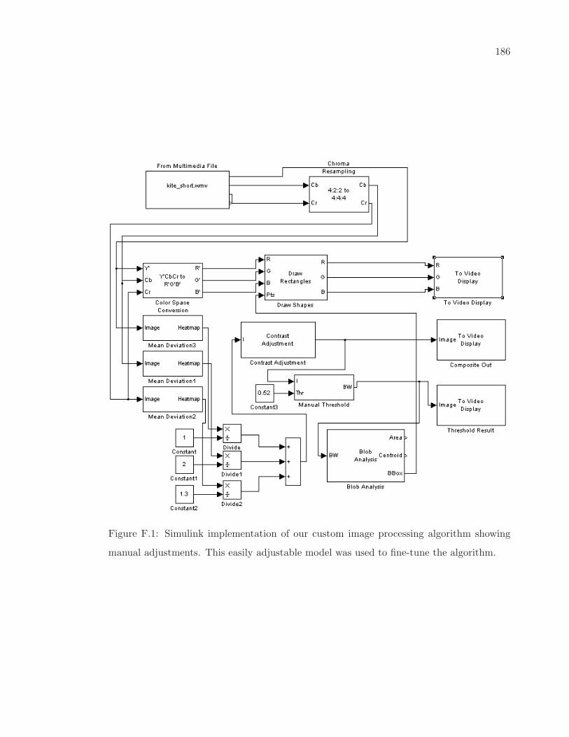
186
Figure F.1: Simulink implementation of our custom image processing algorithm showing
manual adjustments. This easily adjustable model was used to fine-tune the algorithm.
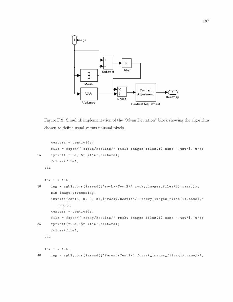
187
Figure F.2: Simulink implementation of the “Mean Deviation” block showing the algorithm
chosen to define usual versus unusual pixels.
centers = centroids;
file = fopen([’field/Results/’ field_images_files(i).name ’.txt ’],’w’);
25 fprintf(file ,’%f %f\n’,centers);
fclose(file);
end
for i = 1:4,
30 img = rgb2ycbcr(imread([’rocky/Test2/’ rocky_images_files(i).name]));
sim Image_processing;
imwrite(cat(3, R, G, B),[’rocky/Results/’ rocky_images_files(i).name],’
png ’);
centers = centroids;
file = fopen([’rocky/Results/’ rocky_images_files(i).name ’.txt ’],’w’);
35 fprintf(file ,’%f %f\n’,centers);
fclose(file);
end
for i = 1:4,
40 img = rgb2ycbcr(imread([’forest/Test2/’ forest_images_files(i).name]));
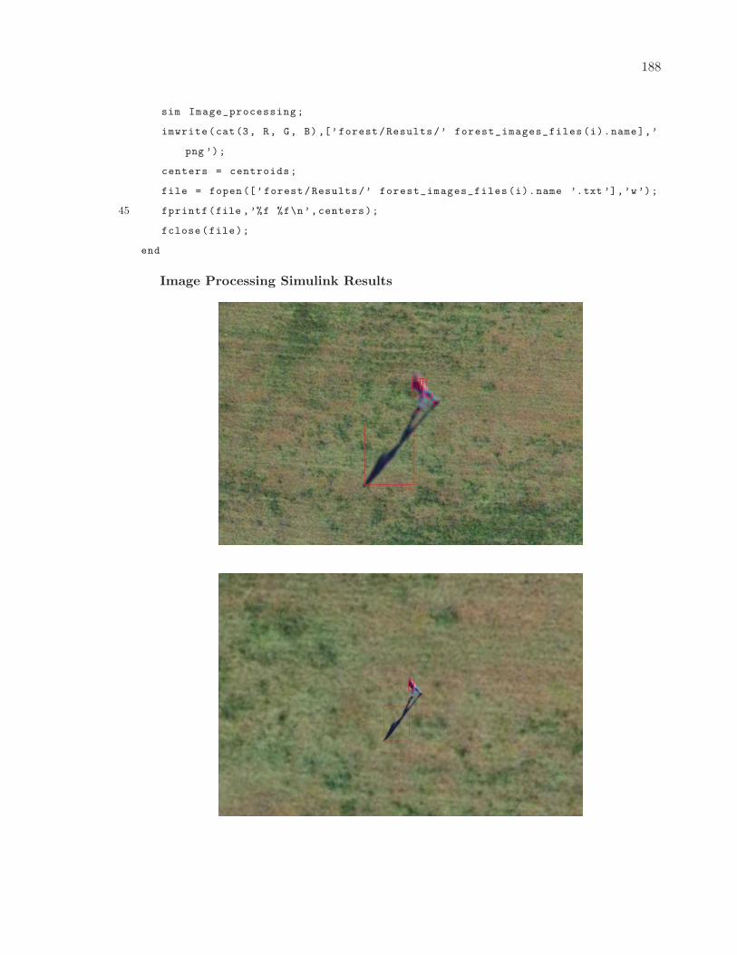
188
sim Image_processing;
imwrite(cat(3, R, G, B),[’forest/Results/’ forest_images_files(i).name],’
png ’);
centers = centroids;
file = fopen([’forest/Results/’ forest_images_files(i).name ’.txt ’],’w’);
45 fprintf(file ,’%f %f\n’,centers);
fclose(file);
end
Image Processing Simulink Results
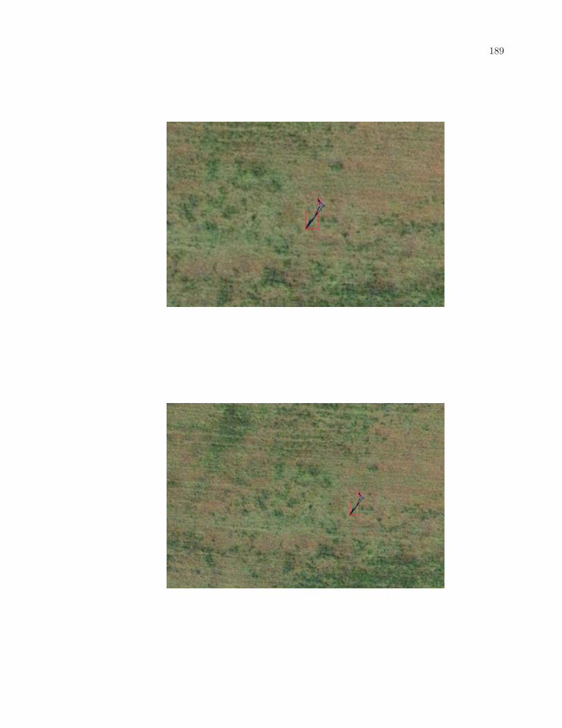
189
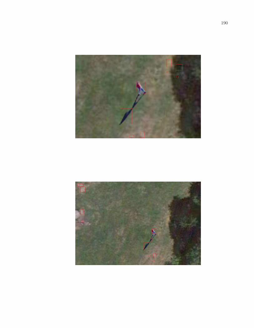
190
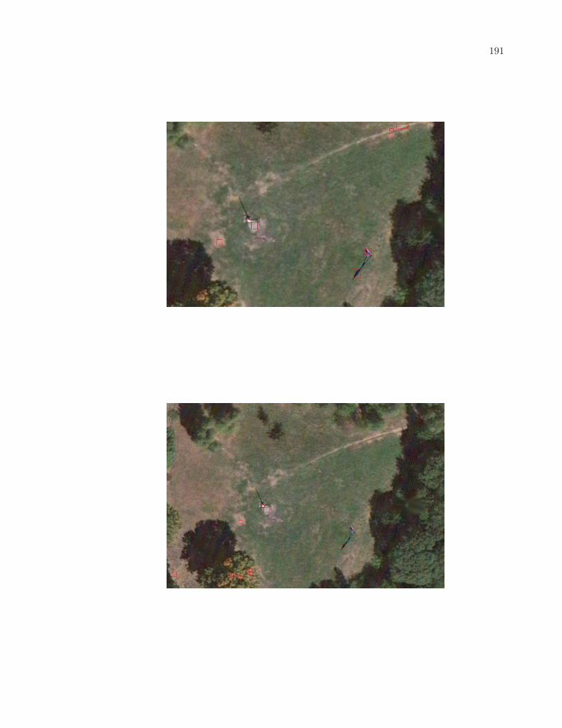
191
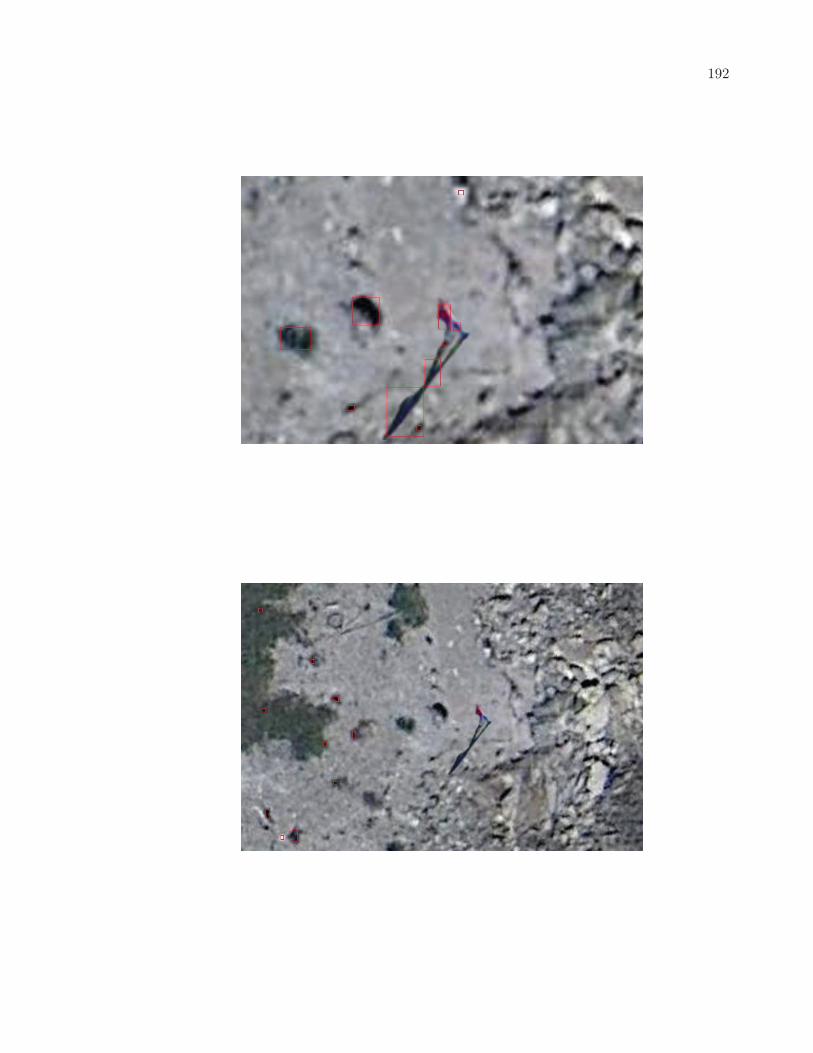
192
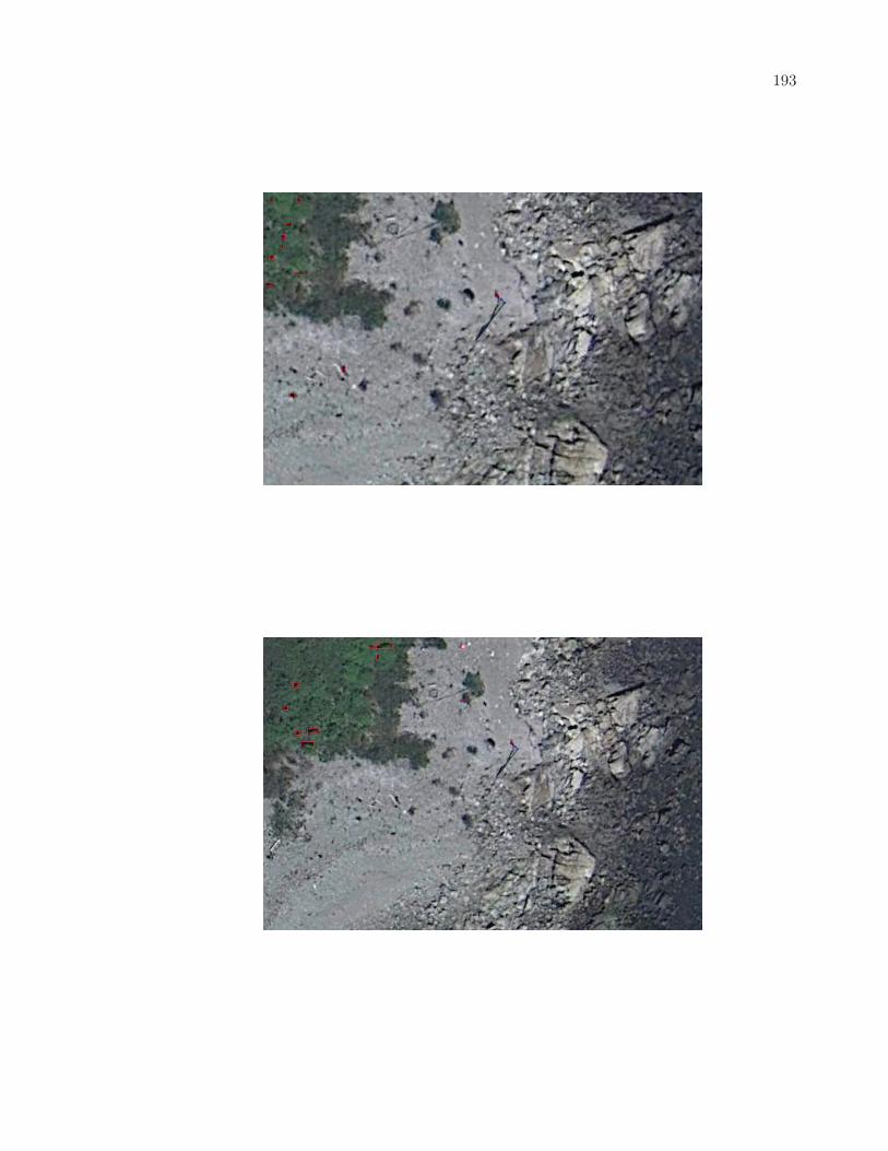
193
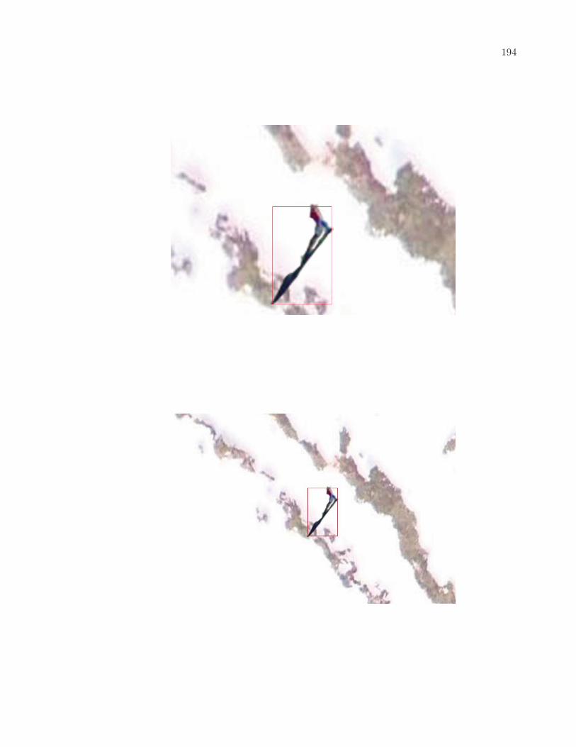
194
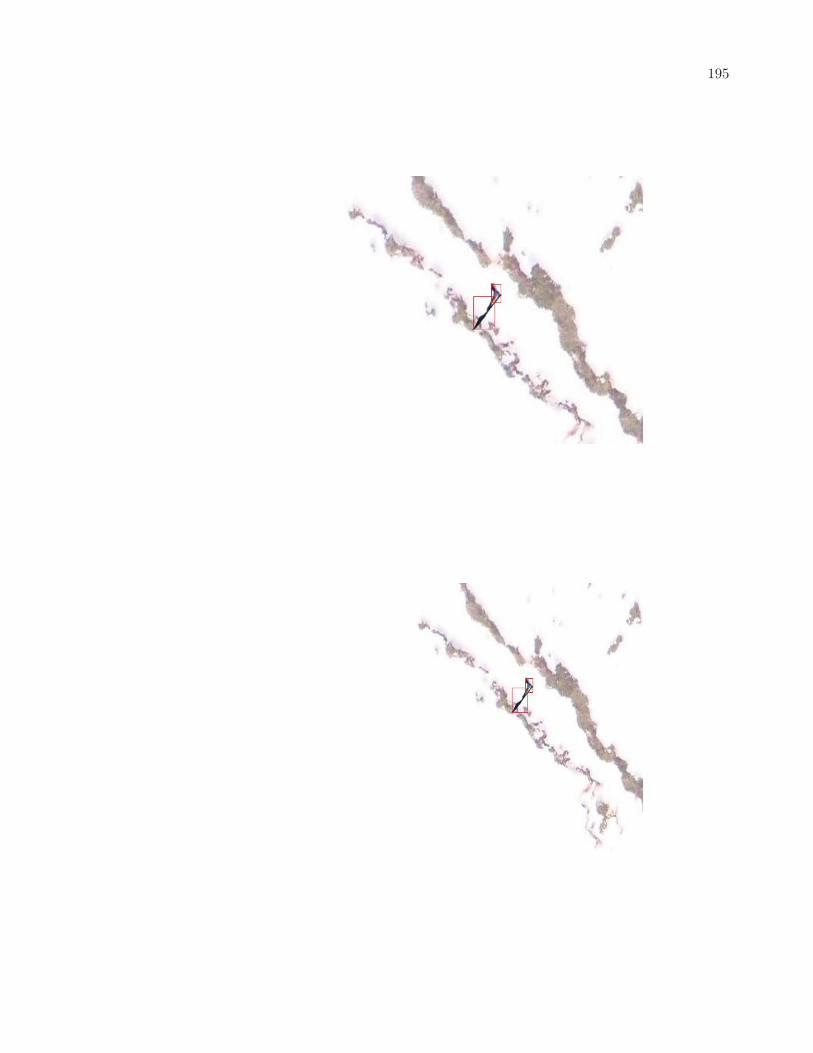
195
196
Bibliography
[1] Unknown. (2011, Nov.) Rescue over louisiana. [Online]. Available: http:
//www.katrinadestruction.com
[2] U. A. F. photo Lt Col Leslie Pratt. (2012) MQ-1 predator unmanned aircraft. [Online].
Available: http://www.af.mil/shared/media/photodb/photos/081131-F-7734Q-001.
jpg
[3] (2012) Brigham young university during dry run of WiSAR UAV. [Online]. Available:
https://facwiki.cs.byu.edu/WiSAR/
[4] dbenzhuser, “Pathfinding a star,” 2006, [Online; accessed 14-Apr-2012].
[Online]. Available: http://upload.wikimedia.org/wikipedia/commons/thumb/f/f4/
Pathfinding A Star.svg/500px-Pathfinding A Star.svg.png
[5] J. Dreo, “The ant colony optimization of the travelling salesman problem,” 2004,
[Online; accessed 22-Nov-2011]. [Online]. Available: http://en.wikipedia.org/wiki/
Travelling salesman problem
[6] S. Asano, T. Maruyama, and Y. Yamaguchi, “Performance comparison of FPGA GPU
and CPU in image processing,” in Field Programmable Logic and Applications, 2009.
FPL 2009. International Conference on, 31 2009-sept. 2 2009, pp. 126 –131.
[7] J. M. Griggs. (2012) Human figure average measurements. [Online]. Available:
http://www.fas.harvard.edu/∼loebinfo/loebinfo/Proportions/humanfigure.html
[8] (2012) Sony fcb-ix45c 18x color block camera. [Online]. Available: http:
//www.goelectronic.com/SONY+FCB-IX45C.html
197
[9] D. Cooper, J. Frost, and R. Q. Robe, “Compatibility of land SAR procedures with
search theory,” Potomac Management Group Inc., Tech. Rep., December 2003.
[10] T. W. Heggie and M. E. Amundson, “Dead men walking: Search and rescue in US
national parks,” Wilderness and Environmental Medicine, vol. 20, pp. 244–249, 2009.
[11] D. A. Graham, “A mountain of bills,” Newsweek, December 2009.
[12] C. Search and R. Board, “Examples of endangered persons refusing SAR help,
waiting to call for help or hiding from help because of fear of large bill”
http://www.coloradosarboard.org/csrb-documents/Refusing, Nov. 2011.
[13] L. Lin, M. Roscheck, M. Goodrich, and B. Morse, “Supporting wilderness
search and rescue with integrated intelligence: Autonomy and information
at the right time and the right place,” 2010. [Online]. Available: https:
//www.aaai.org/ocs/index.php/AAAI/AAAI10/paper/view/1864
[14] J. R. R. Gaemus E. Collins and P. S. Vegdahl, “A uav routing and sensor control
optimization algorithm for target search,” Proceedings of SPIE, 2007. [Online].
Available: http://link.aip.org/link/PSISDG/v6561/i1/p65610D/s1&Agg=doi
[15] L. H. Nunn, “An introduction to the literature of search theory,” CNA Corporation,
Tech. Rep., October 2003.
[16] W. Sheng, “Distributed multi-robot coordination in area exploration,” Robotics
and Autonomous Systems, vol. 54, dec. 2006. [Online]. Available: http:
//dx.doi.org/10.1016/j.robot.2006.06.003
[17] J. Kalomiros and J. Lygouras, “A host co-processor FPGA-based architecture for fast
image processing,” in Intelligent Data Acquisition and Advanced Computing Systems:
Technology and Applications, 2007. IDAACS 2007. 4th IEEE Workshop on, sept. 2007,
pp. 373 –378.
[18] J.-S. Leu, W.-H. Lin, M.-C. Yu, and H.-J. Tzeng, “Recognition assisted dynamic
surveillance system based on OSGi and OpenCV,” in Advanced Communication Tech-
nology 13th International Conference on (ICACT’11), feb. 2011, pp. 83 –87.
198
[19] G. Miller and S. Fels, “Developer-centred interface design for computer vision,” in
Computer Vision Workshops IEEE International Conference on (ICCV’11), nov. 2011,
pp. 437 –444.
[20] V. Shehu and A. Dika, “Using real time computer vision algorithms in automatic atten-
dance management systems,” in Information Technology Interfaces 32nd International
Conference on(ITI’10), june 2010, pp. 397 –402.
[21] “An image search system for uavs,” in NRC Canada’s Advanced Innovation and Part-
nership 2005 Conference((UVS)’05).
[22] J. Oh, E.-J. Im, and K. Yoon, “Optical flow computation on a heterogeneous plat-
form,” in Ubiquitous Robots and Ambient Intelligence 8th International Conference
(URAI’11), nov. 2011, pp. 68 –73.
[23] J. Jung, J. Yun, C.-K. Ryoo, and K. Choi, “Vision based navigation using road-
intersection image,” in Control, Automation and Systems 11th International Confer-
ence (ICCAS’11), oct. 2011, pp. 964 –968.
[24] R. Carnie, R. Walker, and P. Corke, “Image processing algorithms for UAV“sense
and avoid”,” in Robotics and Automation, 2006. ICRA 2006. Proceedings 2006 IEEE
International Conference on, may 2006, pp. 2848 –2853.
[25] M. Jasiunas, D. Kearney, J. Hopf, and G. Wigley, “Image fusion for uninhabited air-
borne vehicles,” in Field-Programmable Technology,Proceedings. 2002 IEEE Interna-
tional Conference (FPT’02), dec. 2002, pp. 348 – 351.
[26] P. Andersson, K. Kuchcinski, K. Nordberg, and P. Doherty, “Integrating a computa-
tional model and a run time system for image processing on a uav,” in Digital System
Design, 2002. Proceedings. Euromicro Symposium on, 2002, pp. 102 – 109.
[27] B. J. Tippetts, “Real-time implementation of vision algorithms for control,
stabilization, and target tracking, for a hovering micro-uav,” 2008. [Online]. Available:
http://contentdm.lib.byu.edu/ETD/image/etd2374.pdf
199
[28] D. Jinghong, D. Yaling, and L. Kun, “Development of image processing system based on
DSP and FPGA,” in Electronic Measurement and Instruments, 2007. 8th International
Conference (ICEMI’07), 16 2007-july 18 2007, pp. 2–791 –2–794.
[29] Y. Lei, Z. Gang, R. Si-Heon, L. Choon-Young, L. Sang-Ryong, and K.-M. Bae, “The
platform of image acquisition and processing system based on dsp and fpga,” in Smart
Manufacturing Application, International Conference (ICSMA’08), april 2008, pp. 470
–473.
[30] M. A. Goodrich, B. S. Morse, D. Gerhardt, J. L. Cooper, M. Quigley, J. A. Adams,
and C. Humphrey, “Supporting wilderness search and rescue using a camera-equipped
mini uav: Research articles,” J. Field Robot., vol. 25, no. 1-2, pp. 89–110, Jan. 2008.
[Online]. Available: http://dx.doi.org/10.1002/rob.v25:1/2
[31] M. A. Goodrich, T. W. McLain, J. D. Anderson, J. Sun, and J. W. Crandall,
“Managing autonomy in robot teams: observations from four experiments,” in
Proceedings of the ACM/IEEE international conference on Human-robot interaction,
ser. HRI ’07. New York, NY, USA: ACM, 2007, pp. 25–32. [Online]. Available:
http://doi.acm.org/10.1145/1228716.1228721
[32] S. Waharte, N. Trigoni, and S. Julier, “Coordinated search with a swarm of uavs,”
in Sensor, Mesh and Ad Hoc Communications and Networks Workshops, 2009. . 6th
Annual IEEE Communications Society Conference (SECON’09), june 2009, pp. 1 –3.
[33] Y. Kuwata, A. Richards, T. Schouwenaars, and J. P. How, “Distributed robust receding
horizon control for multivehicle guidance,” IEEE Transactions on Control Systems
Technology, vol. 15, no. 4, pp. 627–641, July 2007.
[34] Paparazzi. (2012) Paparazzi: The free autopilot. [Online]. Available: http:
//paparazzi.enac.fr/
[35] ENAC. (2012) Enac interactive computing laboratory. [Online]. Available: http:
//www.lii-enac.fr/en/research.html
200
[36] Xilinx. (2012) Xtremedsp 48 slice. [Online]. Available: http://www.xilinx.com/
technology/dsp/xtremedsp.htm
[37] microsoft. (2012) Lifecam cinema. [Online]. Available: http://www.microsoft.com/
hardware/en-us/p/lifecam-cinema/H5D-00001#support
[38] L. Depeche. (2010, May) Pyrnes : mort et prisonnier des
glaces. [Online]. Available: http://www.ladepeche.fr/article/2010/05/24/
841327-pyrenees-mort-et-prisonnier-des-glaces.html
[39] P. D. Community. (2010, May) Hecto. [Online]. Available: http://paparazzi.enac.fr/
wiki/Hecto
[40] T. Instruments. (2012) Pandaboard. [Online]. Available: http://www.pandaboard.org/
[41] ——. (2012) Beagleboard. [Online]. Available: http://beagleboard.org/
[42] R. P. Foundation. (2012) Raspberry pi. [Online]. Available: http://www.raspberrypi.
org/
[43] Newegg. (2012) Intel BOXDH61DLB3 LGA 1155 intel H61 USB 3.0 mini ITX intel
motherboard. [Online]. Available: http://www.newegg.com/Product/Product.aspx?
Item=N82E16813121505
[44] Intel. (2012) Intel desktop boardD525MW. [Online]. Available:
http://www.intel.com/content/www/us/en/motherboards/desktop-motherboards/
desktop-board-d525mw.html
[45] E-ITX. (2012) Axiomtek PICO820 fanless Pico-ITX embedded mainboard, atom Z530
1.6 ghz. [Online]. Available: http://www.e-itx.com/pico820vga-z530.html
[46] Digilent. (2012) Atlys spartan-6 fpga development board. [Online]. Available: http:
//www.digilentinc.com/Products/Detail.cfm?NavPath=2,400,836&Prod=ATLYS
[47] Xilinx. (2012) Avnet spartan-6 lx9 microboard. [Online]. Available: http:
//www.xilinx.com/products/boards-and-kits/AES-S6MB-LX9.htm
201
[48] A. Devices. (2012) BF506F EZ-KIT lite for the ADSP-BF50X blackfin family.
[Online]. Available: http://www.analog.com/en/evaluation/BF506F-EZLITE/eb.
html#ppa print table
[49] T. Instruments. (2012) C5535 ezdsp usb stick development kit. [Online]. Available:
http://www.ti.com/tool/tmdx5535ezdsp
[50] J. Hammes, A. Bohm, C. Ross, M. Chawathe, B. Draper, and W. Najjar,
“High performance image processing on fpgas,” 2001. [Online]. Available:
http://www.cs.colostate.edu/cameron/Publications/hammes lacsi01.pdf
[51] T. B. Nguyen and S. T. Chung, “An improved real-time blob detection for visual
surveillance,” in Image and Signal Processing, 2nd International Congress on (CISP
’09), oct. 2009, pp. 1 –5.
[52] W. Ahmed, M. Irfan, Muzammil, and Yaseen, “Pointing and target selection of object
using color detection algorithm through dsp processor tms320c6711,” in Information
and Communication Technologies International Conference on (ICICT’11), july 2011,
pp. 1 –3.
[53] M.-J. Zhang and W. Gao, “An adaptive skin color detection algorithm with confusing
backgrounds elimination,” in Image Processing, IEEE International Conference on
(ICIP’05), vol. 2, sept. 2005, pp. II – 390–3.
[54] E. Shahinfard, M. Sid-Ahmed, and M. Ahmadi, “A motion adaptive deinterlacing
method with hierarchical motion detection algorithm,” in Image Processing, 2008.
ICIP 2008. 15th IEEE International Conference on, pp. 889 –892.
[55] J. Hao and T. Shibata, “A vlsi-implementation-friendly ego-motion detection algorithm
based on edge-histogram matching,” in Acoustics, Speech and Signal Processing, 2006.
ICASSP 2006 Proceedings. 2006 IEEE International Conference on, vol. 2, may 2006,
p. II.
[56] P. Zhang, T.-Y. Cao, and T. Zhu, “A novel hybrid motion detection algorithm based
202
on dynamic thresholding segmentation,” in Communication Technology 12th IEEE In-
ternational Conference on (ICCT’10), nov. 2010, pp. 853 –856.
[57] X. Chen and H. Chen, “A novel color edge detection algorithm in RGB color space,” in
Signal Processing IEEE 10th International Conference (ICSP’10), oct. 2010, pp. 793
–796.
[58] J. Dreo, “Shortest path find by an ant colony,” 2004, [Online; accessed 14-Apr-2012].
[Online]. Available: http://en.wikipedia.org/wiki/Ant colony optimization algorithms
[59] L. Li, W. Huang, I. Y.-H. Gu, and Q. Tian, “Statistical modeling of complex back-
grounds for foreground object detection,” Image Processing, IEEE Transactions on,
vol. 13, no. 11, pp. 1459 –1472, nov. 2004.
[60] M. Piovoso and P. A. Laplante, “Kalman filter recipes for real-time image processing,”
Real-Time Imaging, vol. 9, pp. 433–439, December 2003. [Online]. Available:
http://dl.acm.org/citation.cfm?id=982353.982359
[61] H. L. Alexander, A. J. Azarbayejani, and H. J. Weigl, “Kalman-filter-based machine
vision for controlling free-flying unmanned remote vehicles,” in American Control Con-
ference, 1992, june 1992, pp. 2006 –2011.
[62] S. Russell and P. Norvig, Artificial Intelligence: A Modern Approach, 3rd ed. New
York: Prentice Hall, 2010.
[63] W. Turri and D. Pointer, “UAV video image stabilization on the SRC map processor,”
jan 2009. [Online]. Available: http://www.srccomp.com/news/docs/HPEC09 Turri.
Recommended