Download pdf - second edition. McGra w-Hill Publishing Compan · Mo del F abrication G. Elb er 20 Assem bly is left to the enjo ymen t of the author and other mo del building en th usiasts. 6 Ac

Model Fabrication G. Elber 22

[16] R. Riesenfeld. Applications of B-spline approximation to Geometric Problems of

Computer-Aided Design. Ph.D. thesis. University of Utah Technical Report UTEC-

CSc-73-126, March 1973.

[17] D. F. Rogers and J. A. Adams. Mathematical Elements for Computer Graphics,

second edition. McGraw-Hill Publishing Company, 1990.


[7] E. Cohen, T. Lyche, and L. Schumaker. Algorithms for Degree Raising for Splines.

ACM Transactions on Graphics, Vol 4, No 3, pp.171-181, July 1986.

[8] E. Cohen, T. Lyche, and R. Riesenfeld. Discrete B-splines and subdivision Tech-

niques in Computer-Aided Geometric Design and Computer Graphics. Computer

Graphics and Image Processing, 14, 87-111 (1980).

[9] M. D. Carmo. Di�erential Geometry of Curves and Surfaces. Prentice-Hall 1976.

[10] I. D. Faux and M. J. Pratt. Computational Geometry for Design and Manufacturing.

[11] G. Elber and E. Cohen. Error Bounded Variable Distance O�set Operator for Free

Form Curves and Surfaces. International Journal of Computational Geometry and

Applications, Vol. 1., No. 1, pp 67-78, March 1991.

[12] G. Elber and E. Cohen. Second Order Surface Analysis Using Hybrid Symbolic and

Numeric Operators Submitted for publication.

[13] G. Elber. Free Form Surface Analysis using a Hybrid of Symbolic and Numeric

Computation. Ph.D. thesis, University of Utah, Computer Science Department,

1992.

[14] T. McCollough. Support for Trimmed Surfaces. M.S. thesis, University of Utah,

Computer Science Department, 1988.

[15] R. Millman and G. Parker. Elements of Di�erential Geometry. Prentice Hill Inc.,

1977.


Assembly is left to the enjoyment of the author and other model building enthusiasts.

6 Acknowledgment

The author is grateful to Elaine Cohen and Mark Bloomenthal for their valuable remarks

on the various drafts of this paper.

References

[1] RE Barnhill, G. Farin, L. Fayard and H. Hagen. Twists, Curvatures and Surface

Interrogation. Computer Aided Design, vol. 20, no. 6, pp 341-346, July/August

1988.

[2] B. O'Neill. Elementary Di�erential Geometry. Academic Press Inc., 1966.

[3] C. Bennis, J. M. Vezien, and G. Iglesias. Piecewise Surface Flattening for Non-

Distorted texture Mapping. Computer Graphics, Vol. 25, Num. 4, Siggraph Jul.

1991.

[4] B. Cobb. Design of Sculptured Surfaces Using The B-spline representation. Ph.D.

thesis, University of Utah, Computer Science Department, June 1984.

[5] E. Cohen. Some Mathematical Tools for a Modeler's Workbench IEEE Computer

Graphics and Applications, pp 63-66, October 1983.

[6] E. Cohen, T. Lyche, and L. Schumaker. Degree Raising for Splines. Journal of

Approximation Theory, Vol 46, Feb. 1986.


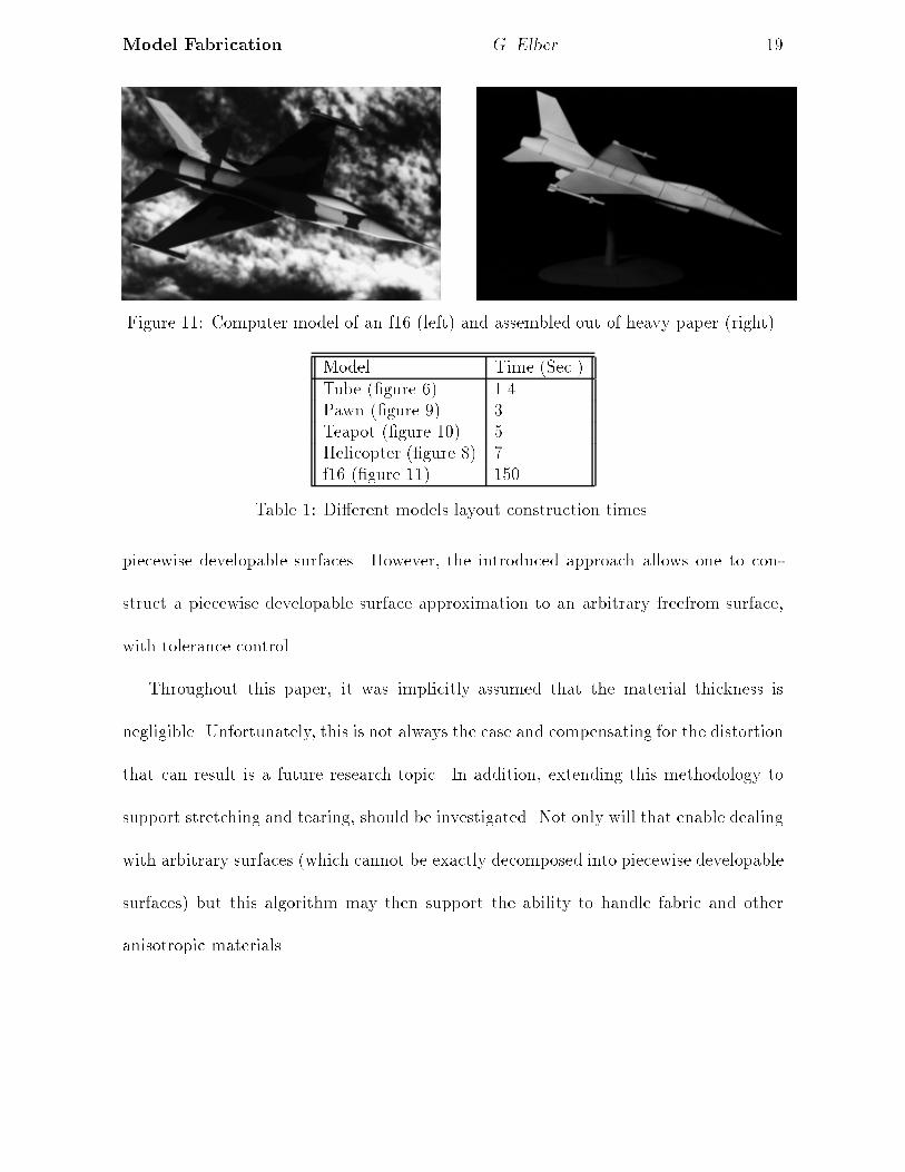
Figure 11: Computer model of an f16 (left) and assembled out of heavy paper (right).

Model Time (Sec.)Tube (�gure 6) 1.4Pawn (�gure 9) 3Teapot (�gure 10) 5Helicopter (�gure 8) 7f16 (�gure 11) 150

Table 1: Di�erent models layout construction times.

piecewise developable surfaces. However, the introduced approach allows one to con-

struct a piecewise developable surface approximation to an arbitrary freefrom surface,

with tolerance control.

Throughout this paper, it was implicitly assumed that the material thickness is

negligible. Unfortunately, this is not always the case and compensating for the distortion

that can result is a future research topic. In addition, extending this methodology to

support stretching and tearing, should be investigated. Not only will that enable dealing

with arbitrary surfaces (which cannot be exactly decomposed into piecewise developable

surfaces) but this algorithm may then support the ability to handle fabric and other

anisotropic materials.


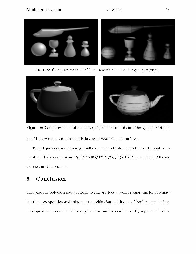
Figure 9: Computer models (left) and assembled out of heavy paper (right).

Figure 10: Computer model of a teapot (left) and assembled out of heavy paper (right).

and 11 show more complex models having several trimmed surfaces.

Table 1 provides some timing results for the model decomposition and layout com-

putation. Tests were run on a SGI4D 240 GTX (R3000 25MHz Risc machine). All tests

are measured in seconds.

5 Conclusion

This paper introduces a new approach to and provides a working algorithm for automat-

ing the decomposition and subsequent speci�cation and layout of freeform models into

developable components. Not every freeform surface can be exactly represented using


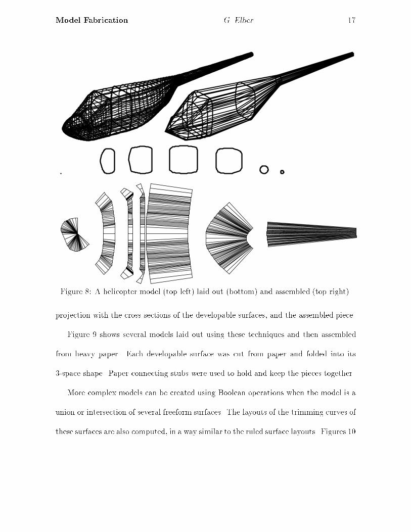
Figure 8: A helicopter model (top left) laid out (bottom) and assembled (top right).

projection with the cross sections of the developable surfaces, and the assembled piece.

Figure 9 shows several models laid out using these techniques and then assembled

from heavy paper. Each developable surface was cut from paper and folded into its

3-space shape. Paper connecting stubs were used to hold and keep the pieces together.

More complex models can be created using Boolean operations when the model is a

union or intersection of several freeform surfaces. The layouts of the trimming curves of

these surfaces are also computed, in a way similar to the ruled surface layouts. Figures 10


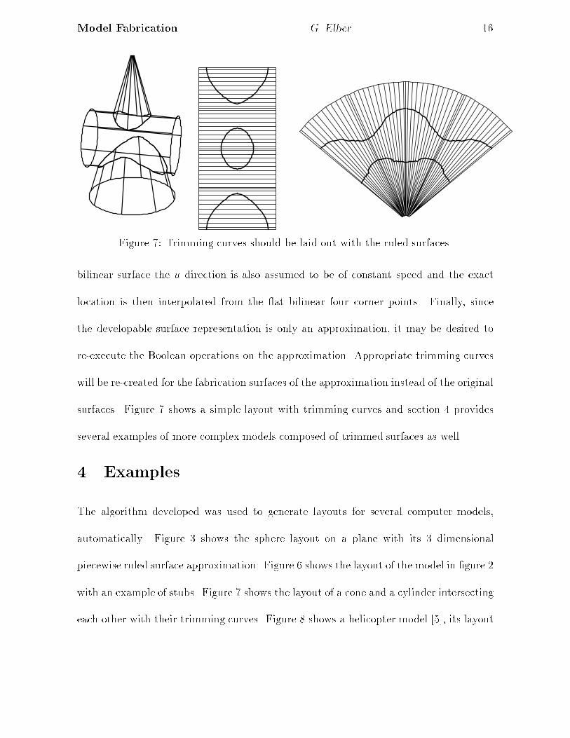
Figure 7: Trimming curves should be laid out with the ruled surfaces.

bilinear surface the u direction is also assumed to be of constant speed and the exact

location is then interpolated from the at bilinear four corner points. Finally, since

the developable surface representation is only an approximation, it may be desired to

re-execute the Boolean operations on the approximation. Appropriate trimming curves

will be re-created for the fabrication surfaces of the approximation instead of the original

surfaces. Figure 7 shows a simple layout with trimming curves and section 4 provides

several examples of more complex models composed of trimmed surfaces as well.

4 Examples

The algorithm developed was used to generate layouts for several computer models,

automatically. Figure 3 shows the sphere layout on a plane with its 3 dimensional

piecewise ruled surface approximation. Figure 6 shows the layout of the model in �gure 2

with an example of stubs. Figure 7 shows the layout of a cone and a cylinder intersecting

each other with their trimming curves. Figure 8 shows a helicopter model [5], its layout


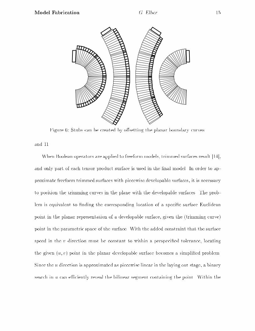
Figure 6: Stubs can be created by o�setting the planar boundary curves.

and 11.

When Boolean operators are applied to freeformmodels, trimmed surfaces result [14],

and only part of each tensor product surface is used in the �nal model. In order to ap-

proximate freeform trimmed surfaces with piecewise developable surfaces, it is necessary

to position the trimming curves in the plane with the developable surfaces. The prob-

lem is equivalent to �nding the corresponding location of a speci�c surface Euclidean

point in the planar representation of a developable surface, given the (trimming curve)

point in the parametric space of the surface. With the added constraint that the surface

speed in the v direction must be constant to within a prespeci�ed tolerance, locating

the given (u; v) point in the planar developable surface becomes a simpli�ed problem.

Since the u direction is approximated as piecewise linear in the laying out stage, a binary

search in u can e�ciently reveal the bilinear segment containing the point. Within the


(a)

(b)

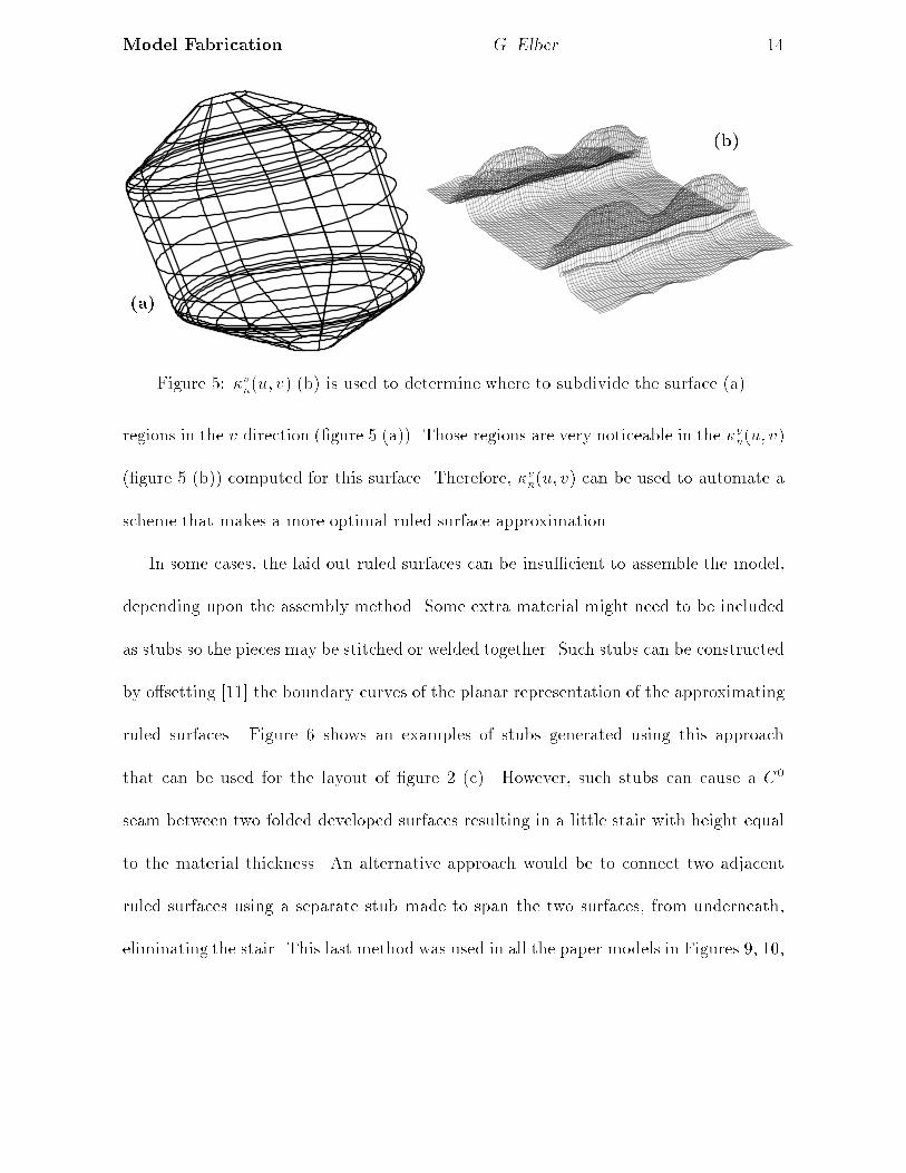
Figure 5: �vn(u; v) (b) is used to determine where to subdivide the surface (a).

regions in the v direction (�gure 5 (a)). Those regions are very noticeable in the �vn(u; v)

(�gure 5 (b)) computed for this surface. Therefore, �vn(u; v) can be used to automate a

scheme that makes a more optimal ruled surface approximation.

In some cases, the laid out ruled surfaces can be insu�cient to assemble the model,

depending upon the assembly method. Some extra material might need to be included

as stubs so the pieces may be stitched or welded together. Such stubs can be constructed

by o�setting [11] the boundary curves of the planar representation of the approximating

ruled surfaces. Figure 6 shows an examples of stubs generated using this approach

that can be used for the layout of �gure 2 (c). However, such stubs can cause a C0

seam between two folded developed surfaces resulting in a little stair with height equal

to the material thickness. An alternative approach would be to connect two adjacent

ruled surfaces using a separate stub made to span the two surfaces, from underneath,

eliminating the stair. This last method was used in all the paper models in Figures 9, 10,


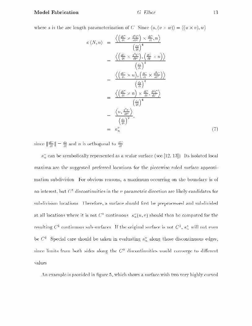
where s is the arc length parameterization of C. Since hu; (v � w)i = h(u� v); wi

� hN;ni =

D�dC

dt� d2C

dt2

�� dC

dt; nE

�ds

dt

�4

=

D�dC

dt� d2C

dt2

�;�dC

dt� n

�E�ds

dt

�4

=

D�dC

dt� n

�;�dC

dt� d2C

dt2

�E�ds

dt

�4

=

D�dC

dt� n

�� dC

dt; d

2C

dt2

E�ds

dt

�4

=

Dn; d

2C

dt2

E�dsdt

�2 ;

= �vn (7)

since kdCdtk = ds

dtand n is orthogonal to dC

dt.

�vn can be symbolically represented as a scalar surface (see [12, 13]). Its isolated local

maxima are the suggested preferred locations for the piecewise ruled surface approxi-

mation subdivision. For obvious reasons, a maximum occurring on the boundary is of

no interest, but C1 discontinuities in the v parametric direction are likely candidates for

subdivision locations. Therefore, a surface should �rst be preprocessed and subdivided

at all locations where it is not C1 continuous. �vn(u; v) should then be computed for the

resulting C1 continuous sub-surfaces. If the original surface is not C2, �vn will not even

be C0. Special care should be taken in evaluating �vn along those discontinuous edges,

since limits from both sides along the C0 discontinuities would converge to di�erent

values.

An example is provided in �gure 5, which shows a surface with two very highly curved


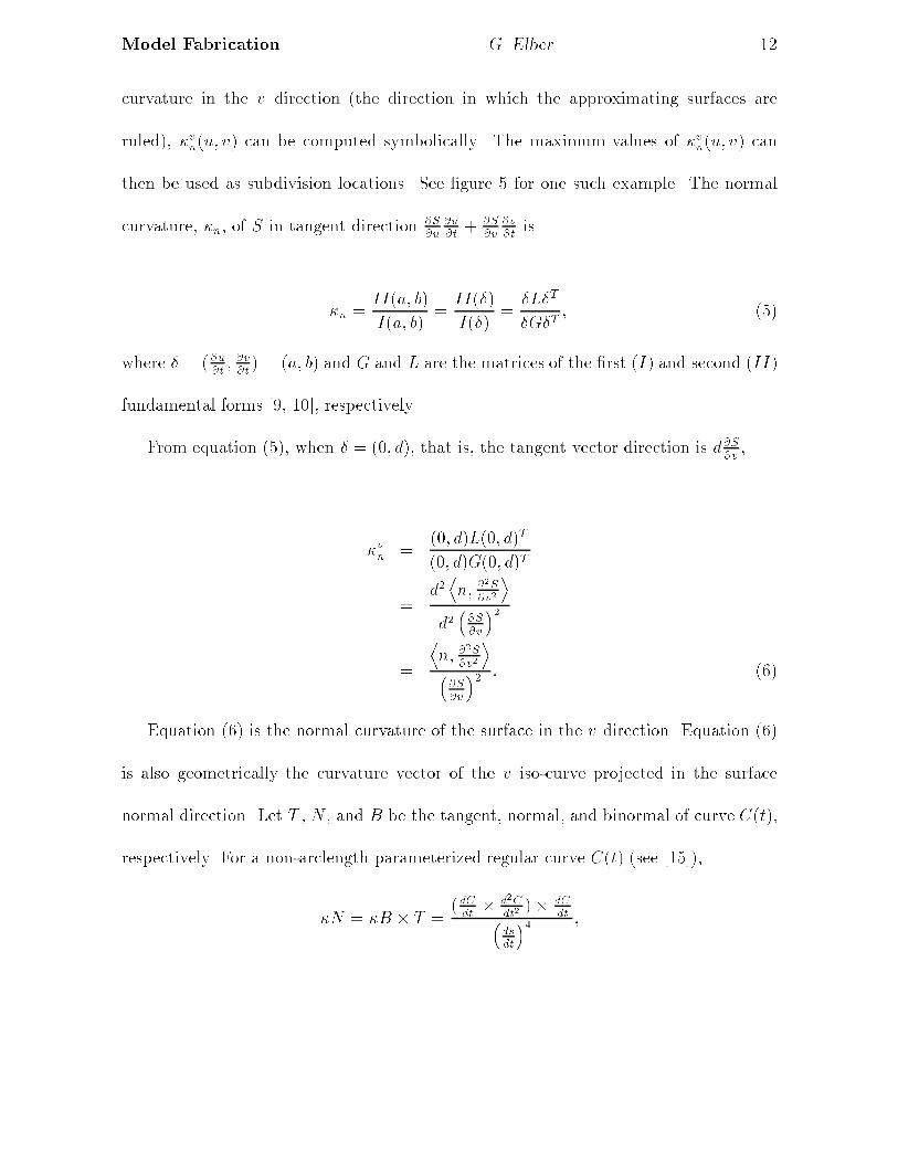
curvature in the v direction (the direction in which the approximating surfaces are

ruled), �vn(u; v) can be computed symbolically. The maximum values of �vn(u; v) can

then be used as subdivision locations. See �gure 5 for one such example. The normal

curvature, �n, of S in tangent direction @S

@u

@u

@t+ @S

@v

@v

@tis

�n =II(a; b)

I(a; b)=

II(�)

I(�)=

�L�T

�G�T; (5)

where � = (@u@t; @v@t) = (a; b) and G and L are the matrices of the �rst (I) and second (II)

fundamental forms [9, 10], respectively.

From equation (5), when � = (0; d), that is, the tangent vector direction is d@S@v,

�vn =(0; d)L(0; d)T

(0; d)G(0; d)T

=d2Dn; @

2S

@v2

Ed2�@S

@v

�2

=

Dn; @

2S

@v2

E�@S

@v

�2 : (6)

Equation (6) is the normal curvature of the surface in the v direction. Equation (6)

is also geometrically the curvature vector of the v iso-curve projected in the surface

normal direction. Let T , N , and B be the tangent, normal, and binormal of curve C(t),

respectively. For a non-arclength parameterized regular curve C(t) (see [15]),

�N = �B � T =(dCdt� d2C

dt2)� dC

dt�dsdt

�4 ;


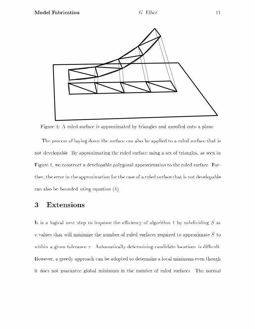
Figure 4: A ruled surface is approximated by triangles and unrolled onto a plane.

The process of laying down the surface can also be applied to a ruled surface that is

not developable. By approximating the ruled surface using a set of triangles, as seen in

Figure 4, we construct a developable polygonal approximation to the ruled surface. Fur-

ther, the error in the approximation for the case of a ruled surface that is not developable

can also be bounded using equation (4).

3 Extensions

It is a logical next step to improve the e�ciency of algorithm 1 by subdividing S at

v values that will minimize the number of ruled surfaces required to approximate S to

within a given tolerance � . Automatically determining candidate locations is di�cult.

However, a greedy approach can be adopted to determine a local minimum even though

it does not guarantee global minimum in the number of ruled surfaces. The normal


so they can be cut out. Lemma 1 can be used to verify whether the piecewise ruled

surfaces are also developable. Since the isometry mapping is nonlinear, in general, an

approximation must be used. We start the process by approximating the two boundary

curves of R that originated on S, C1(u) and C2(u), as piecewise linear curves C1(u) and

C2(u), using re�nement. An identical re�nement should be computed and applied to

both curves to insure they have the same number of linear segments, n. A one-to-one

correspondence between the piecewise linear approximation of each curve is therefore

established. Then, from each pair of corresponding linear segments, one from C1(u) and

one from C2(u), a bilinear surface is created. Each bilinear is further approximated as two

triangles along one of the bilinear diagonals. Finally, the 2n triangles are incrementally

laid out and linearly transformed onto a plane (see �gure 4).

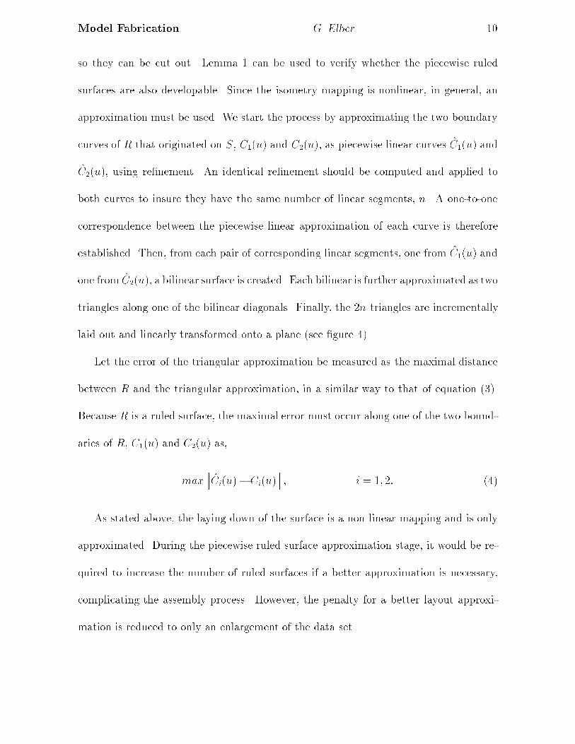
Let the error of the triangular approximation be measured as the maximal distance

between R and the triangular approximation, in a similar way to that of equation (3).

Because R is a ruled surface, the maximal error must occur along one of the two bound-

aries of R, C1(u) and C2(u) as,

max Ci(u)� Ci(u)

; i = 1; 2: (4)

As stated above, the laying down of the surface is a non linear mapping and is only

approximated. During the piecewise ruled surface approximation stage, it would be re-

quired to increase the number of ruled surfaces if a better approximation is necessary,

complicating the assembly process. However, the penalty for a better layout approxi-

mation is reduced to only an enlargement of the data set.


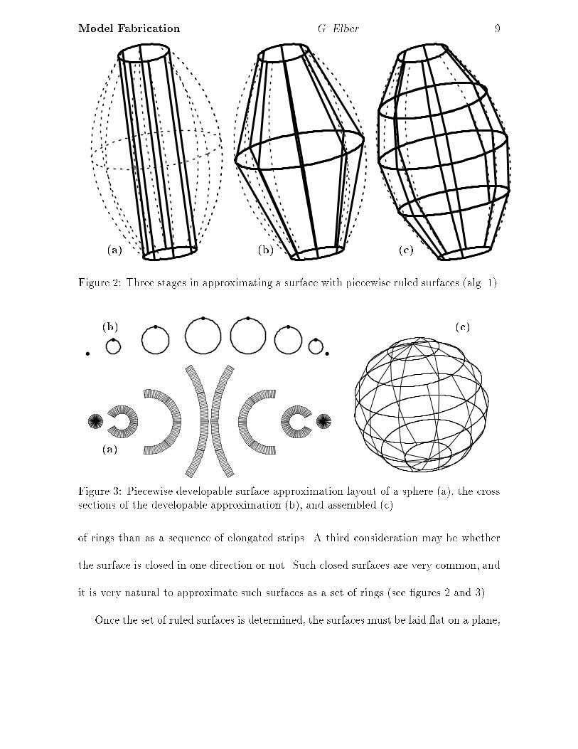
(a) (b) (c)

Figure 2: Three stages in approximating a surface with piecewise ruled surfaces (alg. 1).

(a)

(b) (c)

Figure 3: Piecewise developable surface approximation layout of a sphere (a), the crosssections of the developable approximation (b), and assembled (c).

of rings than as a sequence of elongated strips. A third consideration may be whether

the surface is closed in one direction or not. Such closed surfaces are very common, and

it is very natural to approximate such surfaces as a set of rings (see �gures 2 and 3).

Once the set of ruled surfaces is determined, the surfaces must be laid at on a plane,


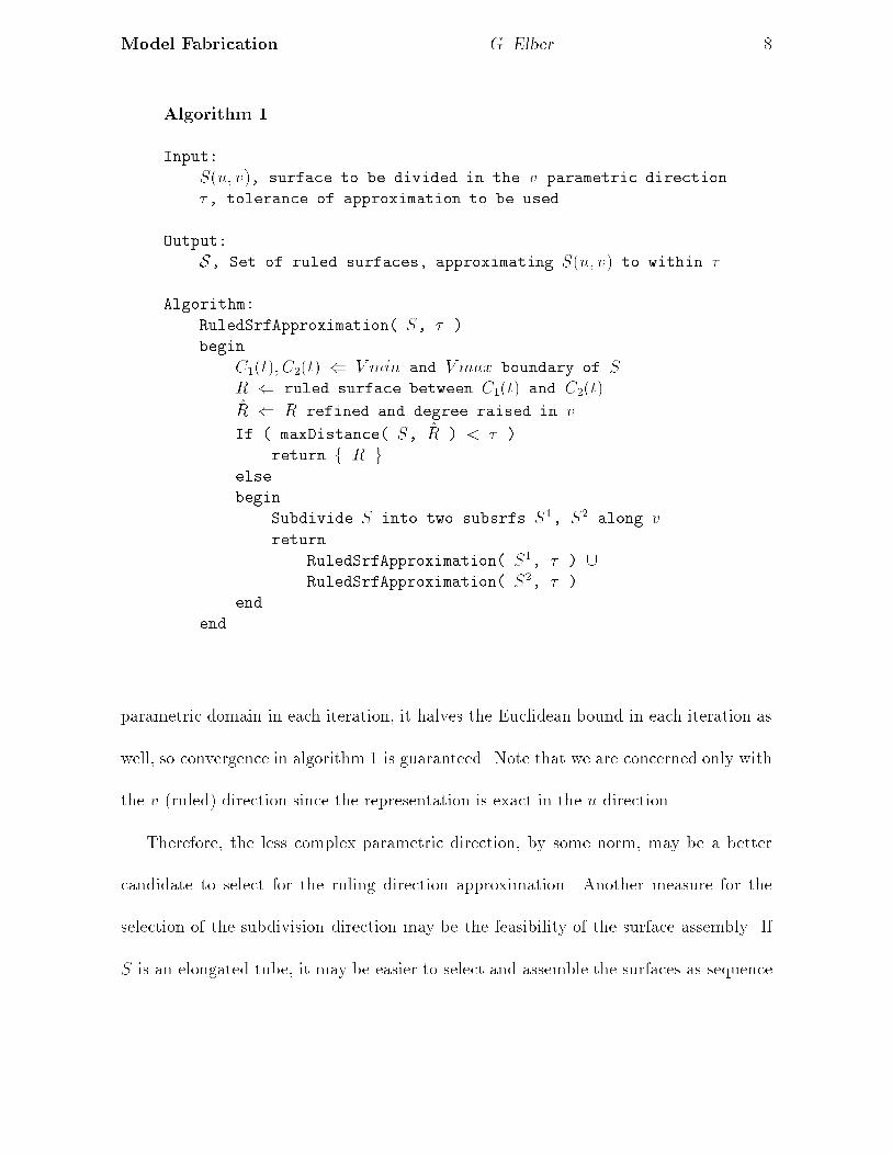
Algorithm 1

Input:

S(u; v), surface to be divided in the v parametric direction.

�, tolerance of approximation to be used.

Output:

S, Set of ruled surfaces, approximating S(u; v) to within �.

Algorithm:

RuledSrfApproximation( S, � )

begin

C1(t); C2(t) ( V min and V max boundary of S.

R ( ruled surface between C1(t) and C2(t).

R ( R refined and degree raised in v.

If ( maxDistance( S, R ) < � )

return f R g.else

begin

Subdivide S into two subsrfs S1, S2 along v.

return

RuledSrfApproximation( S1, � ) [RuledSrfApproximation( S2, � )

end

end

parametric domain in each iteration, it halves the Euclidean bound in each iteration as

well, so convergence in algorithm 1 is guaranteed. Note that we are concerned only with

the v (ruled) direction since the representation is exact in the u direction.

Therefore, the less complex parametric direction, by some norm, may be a better

candidate to select for the ruling direction approximation. Another measure for the

selection of the subdivision direction may be the feasibility of the surface assembly. If

S is an elongated tube, it may be easier to select and assemble the surfaces as sequence


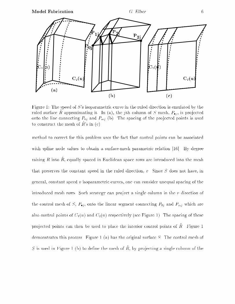
mesh of S, P�j, onto the line connecting P0j and Pmj (b). The new ruled surface, R,

constructed with this new spacing is shown in Figure 1 (c).

The added degree of freedom of a non uniform v speed ruled surface approximation

includes the uniform v speed ruled surface as a special case and so can always be as

good approximation as the uniform speed approximation. Let C1(v) and C2(v) be two

isoparametric curves of S in the v direction. Since we consider only one column of S

mesh, this strategy will be able to emulate S v speed well only if dC1(v)

dv

. dC2(v)dv

is

almost constant for all v. This condition holds fairly well for large classes of surfaces,

but will not necessarily hold for surfaces constructed via highly non-isometric operations

such as a warp [4]. However, it does eliminate the need for degree raising or re�nement

in the construction of R, since the continuity (knot vector) of S in the v direction is

inherited.

A distance bounded algorithm approximating an arbitrary tensor product surface as

a set of ruled surfaces is derived in algorithm 1 based on this process.

Algorithm 1 returns a set of ruled surfaces that approximates the original surface

S to within the required tolerance � . Figure 2 shows an example of three consecutive

stages of algorithm 1.

Assuming S satis�es a Lipschitz condition, which automatically holds for B-spline

surfaces, let (�X�v ,�Y�v ,

�Z�v ) be an upper bound on the �rst partial derivatives of S in

the v direction. Given a �nite range in the v parametric direction, V, a bound on the

Euclidean size is readily available as (V�X�v , V

�Y�v , V

�Z�v ). Since algorithm 1 halves the


(a)

(b) (c)

C1(u) C1(u)

C2(u) C2(u)

P0j

P1jP2j P3j

Figure 1: The speed of S's isoparametric curve in the ruled direction is emulated by theruled surface R approximating it. In (a), the jth column of S mesh, P�j , is projectedonto the line connecting P0j and Pmj (b). The spacing of the projected points is used

to construct the mesh of R's in (c).

method to correct for this problem uses the fact that control points can be associated

with spline node values to obtain a surface-mesh parametric relation [16]. By degree

raising R into R, equally spaced in Euclidean space rows are introduced into the mesh

that preserves the constant speed in the ruled direction, v. Since S does not have, in

general, constant speed v isoparametric curves, one can consider unequal spacing of the

introduced mesh rows. Such strategy can project a single column in the v direction of

the control mesh of S, P�j , onto the linear segment connecting P0j and Pmj which are

also control points of C1(u) and C2(u) respectively (see Figure 1). The spacing of these

projected points can then be used to place the interior control points of R. Figure 1

demonstrates this process. Figure 1 (a) has the original surface S. The control mesh of

S is used in Figure 1 (b) to de�ne the mesh of R, by projecting a single column of the


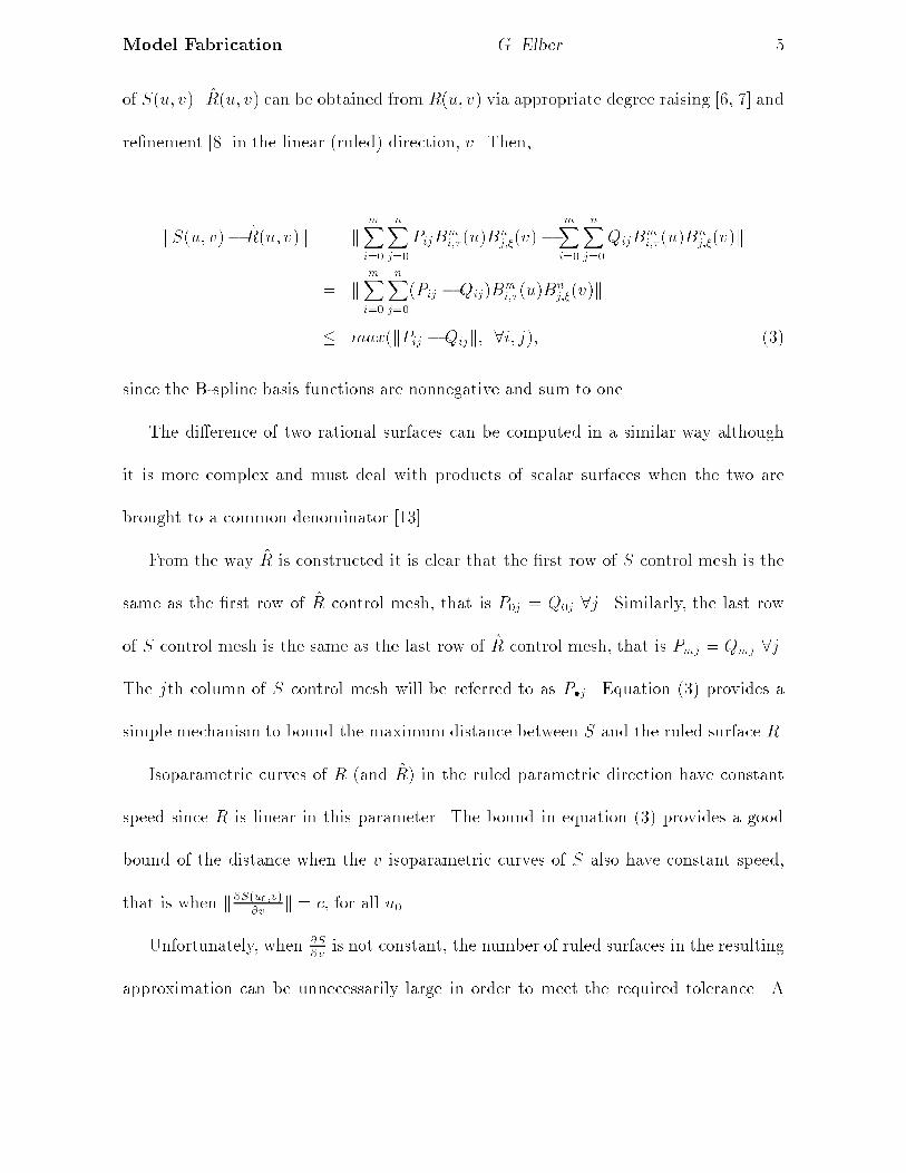
of S(u; v). R(u; v) can be obtained from R(u; v) via appropriate degree raising [6, 7] and

re�nement [8] in the linear (ruled) direction, v. Then,

kS(u; v)� R(u; v)k = kmXi=0

nXj=0

PijBmi;� (u)B

nj;�(v)�

mXi=0

nXj=0

QijBmi;� (u)B

nj;�(v)k

= kmXi=0

nXj=0

(Pij �Qij)Bmi;�(u)B

nj;�(v)k

� max(kPij �Qijk; 8i; j); (3)

since the B-spline basis functions are nonnegative and sum to one.

The di�erence of two rational surfaces can be computed in a similar way although

it is more complex and must deal with products of scalar surfaces when the two are

brought to a common denominator [13].

From the way R is constructed it is clear that the �rst row of S control mesh is the

same as the �rst row of R control mesh, that is P0j = Q0j 8j. Similarly, the last row

of S control mesh is the same as the last row of R control mesh, that is Pmj = Qmj 8j.

The jth column of S control mesh will be referred to as P�j. Equation (3) provides a

simple mechanism to bound the maximum distance between S and the ruled surface R.

Isoparametric curves of R (and R) in the ruled parametric direction have constant

speed since R is linear in this parameter. The bound in equation (3) provides a good

bound of the distance when the v isoparametric curves of S also have constant speed,

that is when k@S(u0;v)@v

k = c, for all u0.

Unfortunately, when @S@v

is not constant, the number of ruled surfaces in the resulting

approximation can be unnecessarily large in order to meet the required tolerance. A


\crosstalk" in the parameterization. Equation (2) measures this \crosstalk" projected

in the direction of the surface normal.

Assuming one can approximate a given surface by a set of disjoint (except along

boundaries) piecewise ruled surfaces within a prescribed tolerance, lemma 1 can be

used to verify that each member of the set of ruled surfaces is also developable. Each

developable surface can then be unfolded, laid at and cut from a planar sheet such as

paper or metal. In section 2, we also consider the case in which a ruled surface is not

developable and present an approximation scheme with a tolerance control. By folding

each laid down surface back to its Euclidean orientation and stitching them all together,

a C0 approximation of the computer model is constructed.

Section 2 develops the background required for this method, and presents the basic

algorithm. In section 3, we investigate several possible extensions including optimization,

stub generation, and handling of trimmed surfaces. Section 4 lays out several examples

including some models assembled from paper.

All the examples throughout this paper were created using an implementation that

is based on the Alpha 1 solid modeler, developed at the University of Utah.

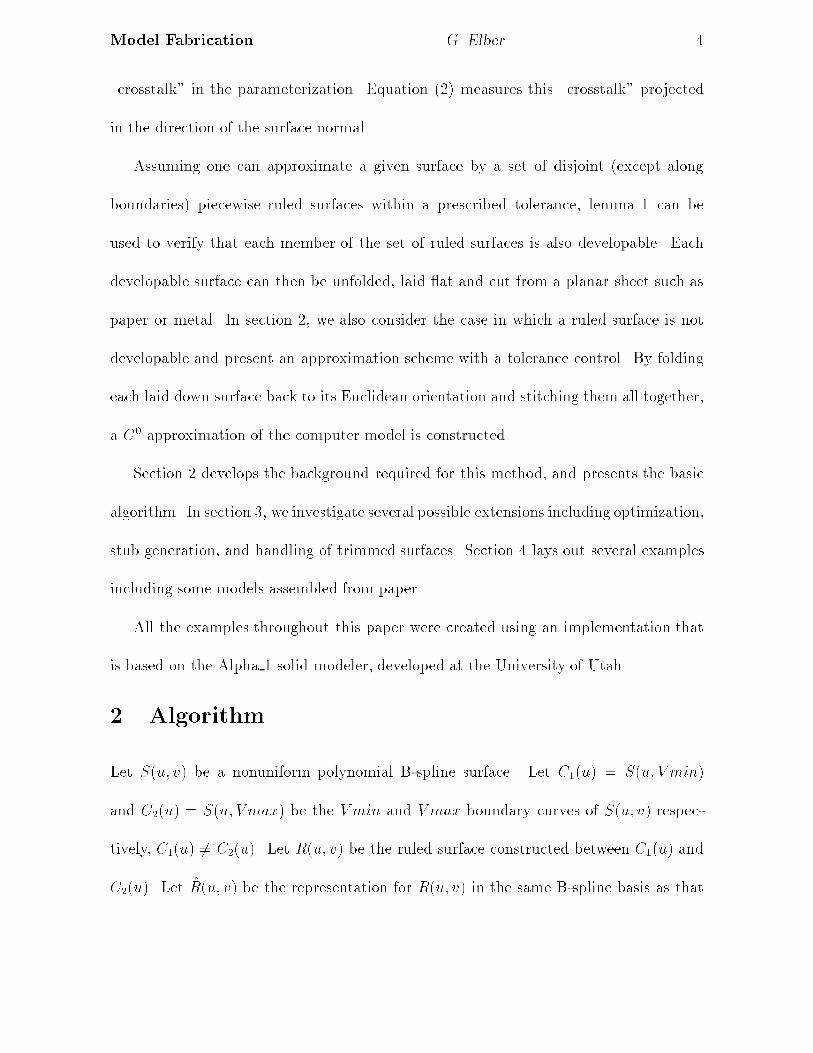
2 Algorithm

Let S(u; v) be a nonuniform polynomial B-spline surface. Let C1(u) = S(u; V min)

and C2(u) = S(u; Vmax) be the V min and V max boundary curves of S(u; v) respec-

tively, C1(u) 6= C2(u). Let R(u; v) be the ruled surface constructed between C1(u) and

C2(u). Let R(u; v) be the representation for R(u; v) in the same B-spline basis as that


�rst concentrate on a superset of it, namely the class of ruled surfaces. In order to be

able to use ruled surfaces instead, we need to derive the conditions in which a ruled

surface is also developable. Let jGj and jLj be the determinants of the �rst and second

fundamental form [2, 9], respectively.

Lemma 1 Let R be a regular ruled surface, R(u; v) = C1(u) � v + C2(u) � (1 � v),

v 2 (0; 1). R is developable if and only ifDnr;

@2R@u@v

E� 0,

Proof: Given a regular surface S, its Gaussian curvature, K, is zero everywhere

(therefore, it is developable) if jLj � 0 since K = jLjjGj, and jGj 6= 0 for regular surfaces.

jLj =

*n;@2S

@u2

+*n;@2S

@v2

+�

*n;

@2S

@u@v

+2

: (1)

By di�erentiating R twice in v, it is clear that @2R@v2

� 0. We can immediately rewrite

jLj as

jLRj = �

*nr;

@2R

@u@v

+2

; (2)

and the result follows.

Therefore, to determine if a ruled surface is developable, one can symbolically com-

pute �(u; v) =Dnr;

@2R

@u@v

E(That is, represent the scalar surface �(u; v) as a polynomial

B�ezier or piecewise-rational NURBs scalar surface. See [12, 13] for more) and make sure

it is zero everywhere within a prescribed tolerance. In other words, using the convex

hull property of the B�ezier and NURBs representations, all the coe�cients of the scalar

surface �(u; v) must be zero within a prescribed tolerance.

The mixed partials, also called the twist of the surface [1, 13], are a measure of the


and to a less extent to fabric-based industries" [17]. Parts of aircrafts and ships are

assembled from piecewise planar sheets unidirectionally bent into their model positions.

Certain fabric and leather objects are made using patterns made from planar sheets.

Since developable surfaces can be unrolled onto a plane without distortion, they can

be cut from planar sheets, bent back into their �nal position, and stitched together.

In [3], a attening approximation is computed for freeform surfaces to eliminate the

distortion in texture mapping. Surfaces are split into patches along feature (geodesic)

lines and approximated as ats. However, we are mainly interested in isometric pro-

jections that preserves intrinsic distances and angles [2, 9]. Physically, such maps only

bend the surface with no stretching, tearing, or distortion. One of the most interesting

properties of developable surfaces is their ability to be laid at on a plane without dis-

tortion by simply unrolling them [9, 10]. Therefore, we would like to generate a surface

approximation using piecewise developable surfaces [9, 10], for which an isometric map

to a plane exists.

Currently, the process that determines how and where to decompose the model re-

quires human ingenuity and does not provide a bound on the accuracy of the approxi-

mation. This paper explores a technique for automatically decomposing the sculptured

model, using a C0 approximation with error bound control, into sets of developable

surfaces.

The Gaussian curvature of a developable surface S(u; v),K, is zero everywhere [9, 10],

i.e. K(u; v) � 0. The class of developable surfaces is di�cult to deal with, so we will

Model Fabrication

using

Surface Layout Projection �

Gershon Elberyz

Department of Computer Science

University of Utah

Salt Lake City, UT 84112 USA

July 8, 1995

Abstract

This paper presents a model fabrication scheme that automatically approxi-

mates a model whose boundary consists of several freeform surfaces by developable

surfaces and then unroll these developable surfaces onto a plane. The model can

then be fabricated by assembling the sets of developable surfaces which have been

cut from planar sheets and rolled back to their proper Euclidean locations. Both

the approximation and the rolling methods can be made arbitrarily precise.

1 Introduction

It is common to �nd freeform surfaces manually approximated and assembled as sets

of piecewise developable surfaces [9]. In general, freeform surfaces are not developable

and cannot be exactly represented as piecewise developable surfaces. Yet, \developable

surfaces are of considerable importance to sheet-metal- or plate-metal-based industries

�This work was supported in part by DARPA (N00014-91-J-4123). All opinions, �ndings, conclusionsor recommendations expressed in this document are those of the authors and do not necessarily re ectthe views of the sponsoring agencies.

yAppreciation is expressed to IBM for partial fellowship support of the author.zCurrent address: Computer Science Department, Technion, Haifa 32000, Israel

1