Search for the Standard Model Higgs boson in the vector
boson fusion-mediated diphoton decay channel using
multivariate analysis techniques
by
David Di Valentino
A thesis submitted to the
Faculty of Graduate and Postdoctoral Affairs
in partial fulfillment of the requirements
for the degree of
Master of Science
Ottawa-Carleton Institute for Physics
Department of Physics
Carleton University
Ottawa, Ontario, Canada
August, 2013
c© copyright
David Di Valentino, 2013
Abstract
A search for the Standard Model Higgs boson in the diphoton decay channel is
presented using multivariate analysis techniques, with a focus on the vector boson
fusion (VBF) production mechanism. Data events are separated into signal (VBF
H → γγ) and background-like categories using a gradient boosted decision tree,
with the optimized analysis applied to the full 2011−2012 dataset, corresponding
to 4.8 fb−1 of√s = 7 TeV pp collisions, and 21 fb−1 of
√s = 8 TeV collisions.
The best fit invariant mass for events categorized as VBF H → γγ is found to be
mH = 123.5 GeV, with a local significance of 2.9σ. The best fit signal strength
for the W,Z-mediated H → γγ decay (VBF + associated production) is found to
be µVBF+VH × B/BSM = 1.72+0.85−0.77 (stat)+0.48
−0.29 (syst)+0.25−0.29 (theory) at mH = 126.8
GeV, which agrees with Standard Model predictions within 2σ.
i

Acknowledgements
I’d like to thank my supervisor Thomas Koffas, as well as my colleagues Dag
Gillberg, Florian Bernlochner, and Jim Lacey for their guidance, advice, patience,
and hard work over these past two years. Your expertise and understanding of
physics are a constant source of inspiration for me, and I hope that someday I’ll
be able to pass on that inspiration in the same way.
I also give my thanks and love to my parents and sisters for their unwavering
love, support, and encouragement in both the good and trying times.
All my love and thanks to Jill for your constant love and support, and for
putting up with all my globetrotting. Your editing skills and knowledge of lan-
guage, as well, were invaluable in helping me craft a sleek and professional piece
of scientific writing.
Thanks also to NSERC and Carleton University, for providing funding for this
research.
ii
Contents
Abstract i
Acknowledgements ii
List of Tables vi
List of Figures viii
1 Introduction 1
1.1 The Standard Model of particle physics . . . . . . . . . . . . . . . . 1
1.2 The Englert-Brout-Higgs mechanism . . . . . . . . . . . . . . . . . 2
1.3 The Large Hadron Collider . . . . . . . . . . . . . . . . . . . . . . . 3
1.4 The ATLAS Detector . . . . . . . . . . . . . . . . . . . . . . . . . . 4
1.5 Higgs boson production . . . . . . . . . . . . . . . . . . . . . . . . . 5
1.6 Higgs boson decays . . . . . . . . . . . . . . . . . . . . . . . . . . . 6
1.7 Motivation of thesis topic . . . . . . . . . . . . . . . . . . . . . . . 8
2 The VBF H → γγ process 11
2.1 What is vector boson fusion? . . . . . . . . . . . . . . . . . . . . . . 11
2.2 What is the H → γγ decay? . . . . . . . . . . . . . . . . . . . . . . 12
2.3 NLO, NNLO QCD and electroweak corrections . . . . . . . . . . . . 13
2.3.1 QCD corrections to VBF production . . . . . . . . . . . . . 14
2.3.2 Two-loop corrections to H → γγ . . . . . . . . . . . . . . . 15
2.4 Kinematics of the VBF H → γγ process . . . . . . . . . . . . . . . 16
2.4.1 VBF tree-level kinematics . . . . . . . . . . . . . . . . . . . 17
2.4.2 Kinematics of the H → γγ decay . . . . . . . . . . . . . . . 18
2.5 Backgrounds . . . . . . . . . . . . . . . . . . . . . . . . . . . . . . . 20
2.5.1 Dijet backgrounds . . . . . . . . . . . . . . . . . . . . . . . . 20
iii
2.5.2 Diphoton backgrounds . . . . . . . . . . . . . . . . . . . . . 22
3 The H → γγ analysis in ATLAS 23
3.1 Photon reconstruction . . . . . . . . . . . . . . . . . . . . . . . . . 23
3.2 Jet reconstruction . . . . . . . . . . . . . . . . . . . . . . . . . . . . 24
3.2.1 Cluster and jet reconstruction . . . . . . . . . . . . . . . . . 24
3.2.2 Jet energy measurement and correction . . . . . . . . . . . . 25
3.2.3 Jet vertex fraction . . . . . . . . . . . . . . . . . . . . . . . 26
3.3 Diphoton candidate selection . . . . . . . . . . . . . . . . . . . . . . 27
3.4 Dijet candidate selection . . . . . . . . . . . . . . . . . . . . . . . . 29
3.5 Event categorization . . . . . . . . . . . . . . . . . . . . . . . . . . 29
4 Introducing the VBF multivariate analysis 31
4.1 Boosted decision trees . . . . . . . . . . . . . . . . . . . . . . . . . 31
4.2 Signal and background modelling . . . . . . . . . . . . . . . . . . . 33
4.2.1 Signal modelling . . . . . . . . . . . . . . . . . . . . . . . . 33
4.2.2 Background modelling . . . . . . . . . . . . . . . . . . . . . 33
4.2.3 Monte Carlo event weights . . . . . . . . . . . . . . . . . . . 34
4.3 Input sample selection . . . . . . . . . . . . . . . . . . . . . . . . . 35
4.3.1 Samples available for the multivariate analysis . . . . . . . . 35
4.3.2 Signal, background sample configuration . . . . . . . . . . . 36
4.3.3 Background training sample selection . . . . . . . . . . . . . 37
4.4 Input variable selection . . . . . . . . . . . . . . . . . . . . . . . . . 39
4.4.1 Deriving a list of discriminating variables . . . . . . . . . . . 39
4.4.2 Optimization of input variables . . . . . . . . . . . . . . . . 42
4.4.3 Final list of input variables . . . . . . . . . . . . . . . . . . . 45
4.4.4 Kolmogorov-Smirnov (overtraining) tests . . . . . . . . . . . 48
4.5 Definition of VBF MVA categories . . . . . . . . . . . . . . . . . . 50
4.6 Distributions of discriminating variables after VBF categorization . 53
4.7 Checking for BDT sculpting in mγγ . . . . . . . . . . . . . . . . . . 57
5 Refining the VBF multivariate analysis 60
5.1 Improving the background model . . . . . . . . . . . . . . . . . . . 60
5.2 Improving benchmark variable selection . . . . . . . . . . . . . . . . 61
5.3 Optimization of the BDT configuration . . . . . . . . . . . . . . . . 64
5.4 Final definition of VBF MVA categories . . . . . . . . . . . . . . . 67
iv
5.5 Distributions of discriminating variables after categorization . . . . 69
5.6 Checking for BDT sculpting in mγγ . . . . . . . . . . . . . . . . . . 75
6 Systematic uncertainties 78
6.1 Theoretical uncertainties . . . . . . . . . . . . . . . . . . . . . . . . 78
6.1.1 Higher-order perturbative uncertainty for gg → H + 2 jets . 78
6.1.2 Modelling uncertainties of ηZeppγγ . . . . . . . . . . . . . . . . 81
6.1.3 Modelling uncertainties of ∆φjj . . . . . . . . . . . . . . . . 82
6.1.4 Underlying event uncertainty . . . . . . . . . . . . . . . . . 83
6.2 Jet and detector modelling uncertainties . . . . . . . . . . . . . . . 84
6.2.1 Jet energy scale and resolution . . . . . . . . . . . . . . . . . 84
6.2.2 Jet vertex fraction selection . . . . . . . . . . . . . . . . . . 85
7 VBF multivariate analysis results 88
7.1 Analysis goals . . . . . . . . . . . . . . . . . . . . . . . . . . . . . . 88
7.2 Training samples and BDT response . . . . . . . . . . . . . . . . . 91
7.3 mγγ measurement . . . . . . . . . . . . . . . . . . . . . . . . . . . . 93
7.4 Signal strength measurement . . . . . . . . . . . . . . . . . . . . . . 93
8 Conclusions 97
References 99
A Photon, jet reconstruction miscellanea 108
A.1 Definitions of discriminating variables . . . . . . . . . . . . . . . . . 108
A.2 Comparison of background samples after dijet selection . . . . . . . 110
A.3 Descriptions of JES uncertainties . . . . . . . . . . . . . . . . . . . 115
B Personal contributions to the ATLAS collaboration 116
v
List of Tables
4.1 Different types of diphoton + dijet backgrounds tested, and their
composition. . . . . . . . . . . . . . . . . . . . . . . . . . . . . . . . 38
4.2 The top ten most discriminating variables for the preliminary VBF
vs. inverted isolation BDT training, ranked according to signal/background
shape separation and importance. . . . . . . . . . . . . . . . . . . . 42
4.3 Evolution of optimal significance when selecting k variables only
from 10-variable ‘Selection A’. The significance shown is calculated
using the shape method, with statistical and fit uncertainties in-
cluded as penalty terms. . . . . . . . . . . . . . . . . . . . . . . . . 49
4.4 Evolution of optimal significance when selecting k variables only
from 8-variable ‘Selection B’. The significance shown is calculated
using the shape method, with statistical and fit uncertainties in-
cluded as penalty terms. . . . . . . . . . . . . . . . . . . . . . . . . 49
4.5 Signal and background statistics for the VBF vs. inverted isolation
training. . . . . . . . . . . . . . . . . . . . . . . . . . . . . . . . . 51
4.6 Definitions of the high and low VBF categories, along with the
optimal significance and VBF purity obtained for each cut, for the
BDT trained on VBF H → γγ signal Monte Carlo and inverted
isolation background. . . . . . . . . . . . . . . . . . . . . . . . . . . 53
vi
5.1 Separation and importance for each variable used in the eight-
variable VBF vs. Sherpa + inverted isolation training. . . . . . . . . 63
5.2 Configurable parameters for boosted decision trees in TMVA. . . . 64
5.3 Possible values of each parameter tested for BDT configuration scan. 66
5.4 Signal and background statistics for the eight-variable VBF vs.
Sherpa + inverted isolation training. The figures here are quoted
after cuts on ∆ηjj > 2 and |ηZeppγγ | < 5. Notably, the differences in
sample statistics relative to Table 4.5 are due to the additional cut
on |ηZeppγγ |, and the addition of another Sherpa sample (e1264). . . 68
5.5 Definitions of the optimal high and low VBF categories, along with
the optimal significance and VBF purity obtained for each cut, for
the BDT trained on VBF signal and Sherpa + inverted isolation
background. . . . . . . . . . . . . . . . . . . . . . . . . . . . . . . . 69
6.1 Higher-order perturbative correction uncertainties for gg → H for
the high and low VBF categories. . . . . . . . . . . . . . . . . . . . 80
6.2 Underlying event uncertainties for mH = 125 GeV ggF and VBF
Monte Carlo at√s = 8 TeV. . . . . . . . . . . . . . . . . . . . . . . 84
6.3 Largest JES uncertainties for√s = 8 TeV VBF and ggF H →
γγ Monte Carlo samples (mH = 125 GeV). . . . . . . . . . . . . . . 86
6.4 Jet energy resolution uncertainties for√s = 8 TeV VBF, ggF H →
γγ Monte Carlo samples (mH = 125 GeV). . . . . . . . . . . . . . . 86
6.5 Jet vertex fraction systematic uncertainties computed using mH =
125 GeV H → γγ signal Monte Carlo samples at√s = 8 TeV. . . . 86
A.1 Definitions of the kinematic variables used in this analysis. . . . . . 109
A.2 Descriptions of the largest contributors to the JES uncertainty. . . . 115
vii

List of Figures
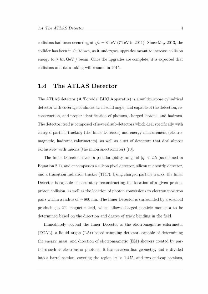
1.1 Tree-level Feynman diagrams of the four main Higgs boson produc-
tion mechanisms at the LHC. . . . . . . . . . . . . . . . . . . . . . 6
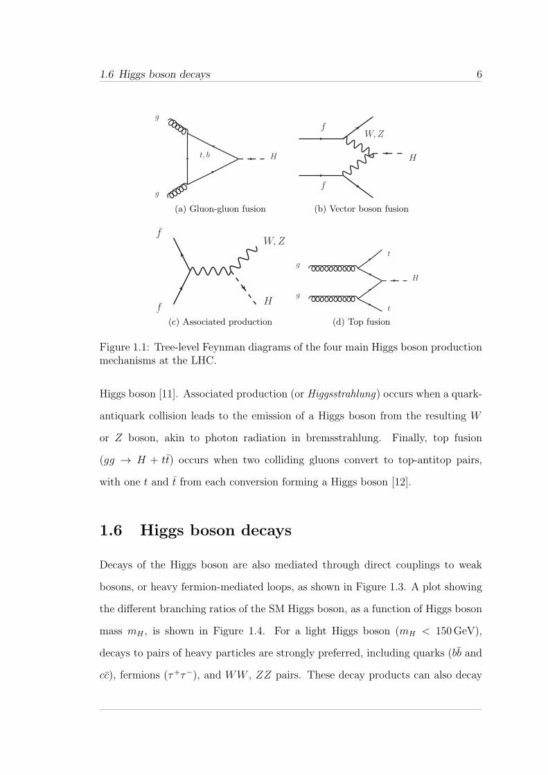
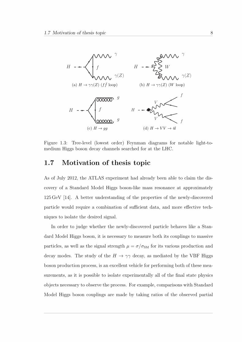
1.2 Standard Model Higgs boson production cross sections for pp colli-
sions at√s = 8TeV. . . . . . . . . . . . . . . . . . . . . . . . . . . 7
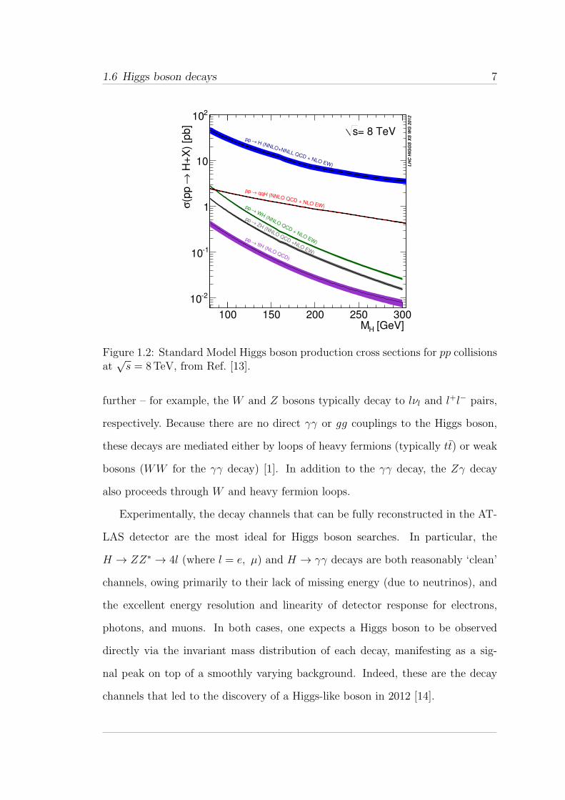
1.3 Tree-level (lowest order) Feynman diagrams for notable light-to-
medium Higgs boson decay channels searched for at the LHC. . . . 8
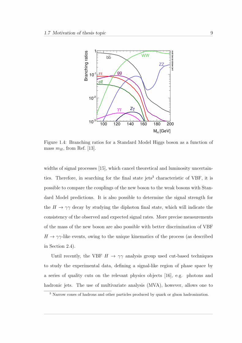
1.4 Branching ratios for a Standard Model Higgs boson as a function
of mass mH . . . . . . . . . . . . . . . . . . . . . . . . . . . . . . . . 9
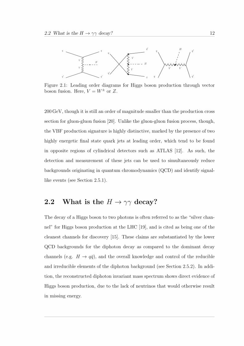
2.1 Leading order diagrams for Higgs boson production through vector
boson fusion. Here, V = W± or Z. . . . . . . . . . . . . . . . . . . 12
2.2 Lowest order contributions to the H → γγ decay cross section. . . . 13
2.3 Feynman diagrams for common NLO QCD corrections to the vector
boson fusion vertex. . . . . . . . . . . . . . . . . . . . . . . . . . . . 14
2.4 Feynman diagrams for NNLO QCD corrections to the vector boson
fusion vertex included in the structure function approach. These
are the only NNLO diagrams found to contribute non-negligibly to
the VBF production cross section. . . . . . . . . . . . . . . . . . . . 15
2.5 Two-loop electroweak corrections for the H → γγ decay process. . . 15
viii
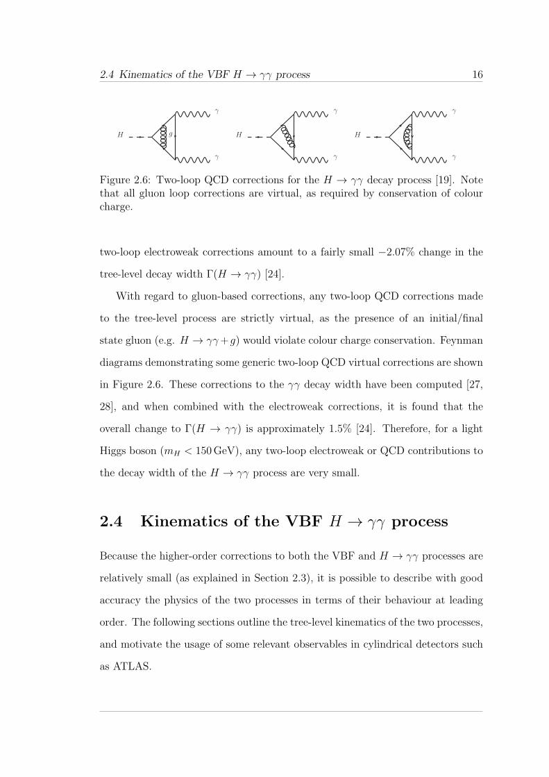
2.6 Two-loop QCD corrections for the H → γγ decay process. Note
that all gluon loop corrections are virtual, as required by conserva-
tion of colour charge. . . . . . . . . . . . . . . . . . . . . . . . . . . 16
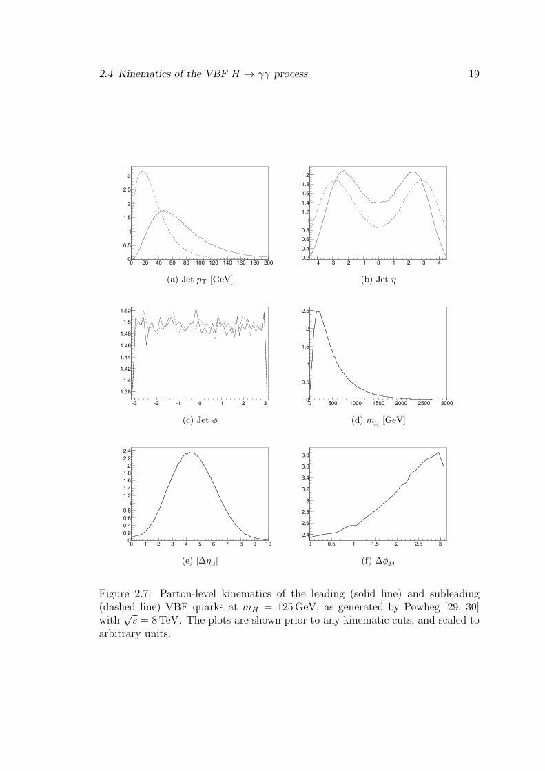
2.7 Parton-level kinematics of the leading (solid line) and subleading
(dashed line) VBF quarks at mH = 125GeV, as generated by
Powheg with√s = 8TeV. The plots are shown prior to any kine-
matic cuts, and scaled to arbitrary units. . . . . . . . . . . . . . . . 19
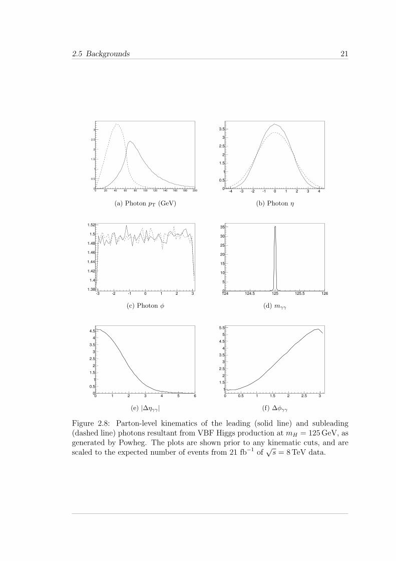
2.8 Parton-level kinematics of the leading (solid line) and subleading
(dashed line) photons resultant from VBF Higgs production at
mH = 125GeV, as generated by Powheg. The plots are shown
prior to any kinematic cuts, and are scaled to the expected number
of events from 21 fb−1 of√s = 8TeV data. . . . . . . . . . . . . . . 21
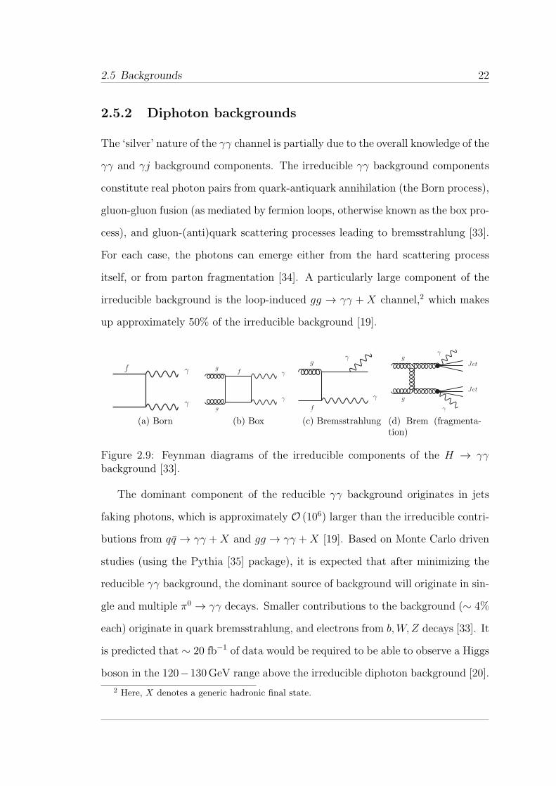
2.9 Feynman diagrams of the irreducible components of the H → γγ
background. . . . . . . . . . . . . . . . . . . . . . . . . . . . . . . . 22
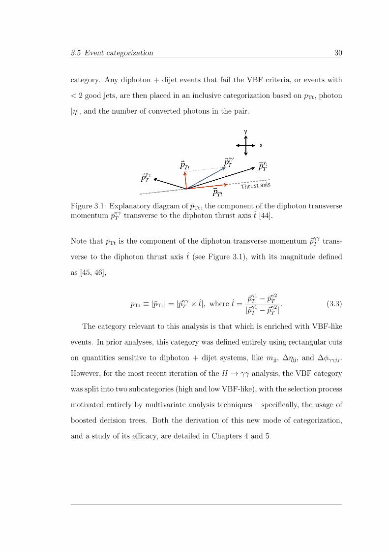
3.1 Explanatory diagram of pTt, the magnitude of the component of
the diphoton transverse momentum ~pγγT transverse to the diphoton
thrust axis t. . . . . . . . . . . . . . . . . . . . . . . . . . . . . . . 30
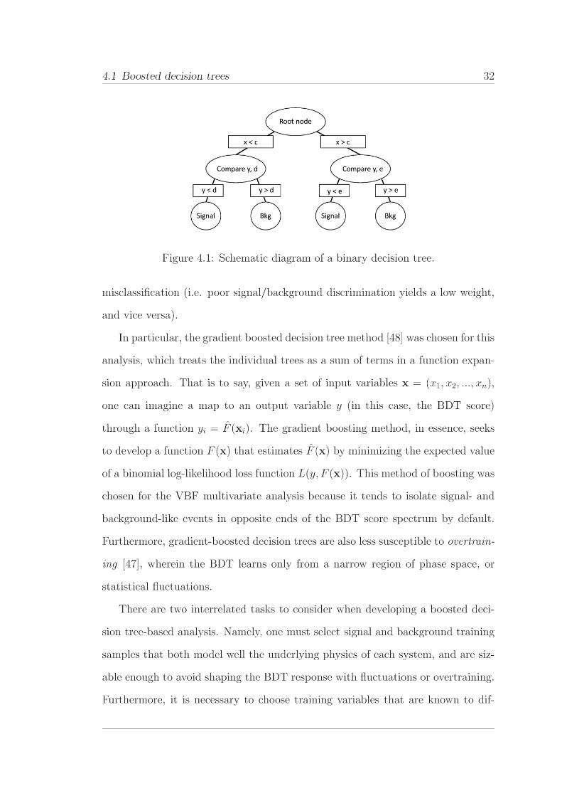
4.1 Schematic diagram of a binary decision tree. . . . . . . . . . . . . . 32
4.2 The distribution of ∆φγγjj in the mH = 125GeV VBF H →
γγ Monte Carlo sample (Powheg + Pythia8) after binning on [2.94, π]. 41
4.3 Distributions ofmγγ for the optimal permutations of variables (pass-
ing the BDT cut) derived from ‘Selection A’ (top) and ‘Selection
B’ (bottom). . . . . . . . . . . . . . . . . . . . . . . . . . . . . . . . 46
4.4 Matrices of the linear correlation coefficients for the optimized sig-
nificance of ‘Selection A’ for signal (left) and background (right). . . 47
ix
4.5 (a) Results of Kolmogorov-Smirnov tests performed by TMVA for
the signal/background training and testing samples. (b) A compar-
ison of the BDT score distributions of the inverted isolation and
data sideband samples after BDT training and application. . . . . . 48
4.6 Hierarchical structure of event selection in the VBF H → γγ mul-
tivariate analysis. . . . . . . . . . . . . . . . . . . . . . . . . . . . . 50
4.7 Distributions of the six benchmark variables for events falling in the
low VBF category (0.18 < BDT score < 0.74) based on the VBF
vs. inverted isolation BDT. Shown here are data sidebands, along
with VBF and ggF H → γγ signal Monte Carlo samples. . . . . . . 55
4.8 Distributions of the six benchmark variables for events falling in
the high VBF category (BDT score > 0.74) based on the VBF vs.
inverted isolation BDT. Shown here are data sidebands, along with
VBF and ggF H → γγ signal Monte Carlo samples. . . . . . . . . . 55
4.9 Comparisons of the benchmark variable distributions of data side-
band and inverted isolation events falling in the low VBF category
(0.18 < BDT score < 0.74) based on the VBF vs. inverted isolation
BDT. . . . . . . . . . . . . . . . . . . . . . . . . . . . . . . . . . . 56
4.10 Comparisons of the benchmark variable distributions of data side-
band and inverted isolation events falling in the high VBF category
(BDT score > 0.74) for the VBF vs. inverted isolation BDT. . . . . 56
4.11 (Top) Plots of the mγγ sidebands for each quartile of VBF signal
Monte Carlo events based on the VBF vs. inverted isolation BDT.
(Bottom) Plots of the mγγ sidebands for each quartile of sideband
data. . . . . . . . . . . . . . . . . . . . . . . . . . . . . . . . . . . . 58
4.12 Profiles of the average BDT score with mγγ. . . . . . . . . . . . . . 59
x
5.1 Comparison of data sidebands with Sherpa + inverted isolation, in-
verted isolation background samples for the six benchmark variables
(Note: All plots have a cut of ∆ηjj > 2 applied). . . . . . . . . . . 62
5.2 Signal (left) and background (right) correlation matrices for VBF
vs. Sherpa + inverted isolation, with cuts on ∆ηjj and ηZeppγγ . . . . . 68
5.3 (a) Kolmogorov-Smirnov test results for the eight-variable train-
ing using VBF H → γγ signal Monte Carlo events vs. Sherpa +
inverted isolation background. (b) The resultant BDT score dis-
tributions for the Sherpa + inverted isolation background training
sample, and data sidebands. . . . . . . . . . . . . . . . . . . . . . . 69
5.4 Distributions of the eight training variables for events in the op-
timized low VBF category (0.51 < BDT score < 0.75) for data
sidebands, and VBF, ggF signal Monte Carlo samples. . . . . . . . 71
5.5 Distributions of the eight benchmark variables for events in the op-
timized high VBF category (BDT score > 0.75) for data sidebands,
and VBF, ggF signal Monte Carlo samples. . . . . . . . . . . . . . . 72
5.6 Comparisons of the benchmark variable distributions of data side-
band and Sherpa + inverted isolation events in the low VBF cate-
gory (0.51 < BDT score < 0.74) for the VBF vs. Sherpa + inverted
isolation BDT. . . . . . . . . . . . . . . . . . . . . . . . . . . . . . 73
5.7 Comparisons of the benchmark variable distributions of data side-
band and Sherpa + inverted isolation events in the high VBF cat-
egory (BDT score > 0.74) for the VBF vs. Sherpa + inverted iso-
lation, eight-variable BDT. . . . . . . . . . . . . . . . . . . . . . . . 74
xi
5.8 (Top) Plots of the mγγ sidebands for each VBF signal Monte Carlo
event quartile for the VBF vs. Sherpa + inverted isolation BDT.
(Bottom) Plots of the mγγ sidebands for each quartile of sideband
data. . . . . . . . . . . . . . . . . . . . . . . . . . . . . . . . . . . . 76
5.9 Profiles of the average BDT score with mγγ. . . . . . . . . . . . . . 77
6.1 Higher-order perturbative uncertainty error bands in the gg →
H + 2-jet decay relative to π −∆φγγjj, derived using the Stewart-
Tackmann procedure. Good agreement is observed between errors
derived from MCFM and Powheg + Pythia8 Monte Carlo. . . . . . 80
6.2 The ratio of the distributions of ηZeppγγ between Powheg + Pythia8
and MCFM (shown on the y-axis), along with the fitted polynomial
reweighting function. . . . . . . . . . . . . . . . . . . . . . . . . . . 82
6.3 Weight function for truth-level ∆φjj (as shown on the y-axis) de-
rived using Sherpa and Powheg + Pythia8. . . . . . . . . . . . . . . 83
6.4 Reweighting functions between CT10 and non-MPI for ggF (left)
and VBF (right) H → γγ Monte Carlo generated using Powheg +
Pythia8. . . . . . . . . . . . . . . . . . . . . . . . . . . . . . . . . . 84
7.1 (a) BDT response of the background sample, as compared to ex-
perimental data, after diphoton + 2-jet + pre-selection cuts. (b)
BDT response of the background and VBF signal samples. . . . . . 92
7.2 The full 2012 mγγ distributions, along with expected SM signal and
background fit for mH = 126.8GeV for low (left) and high (right)
VBF categories. . . . . . . . . . . . . . . . . . . . . . . . . . . . . . 94
xii
7.3 (a) The observed local p0 value for VBF H → γγ events as a func-
tion of mH for the combination of√s = 7TeV and
√s = 8TeV
data. (b) The best-fit values of µggH+ttH × B/BSM and µVBF+VH ×
B/BSM and their 68% (solid) and 95% (dashed) CL contours. . . . 96
A.1 (Left) The layout of the ATLAS detector in Cartesian coordinates,
with definitions of θ and φ, relative to their rotational axes. (Right)
A diagram of pseudorapidity as it relates to the z-axis in ATLAS. . 108
A.2 A comparison of the distributions for inverted isolation, inverted
ID, and Sherpa background samples, along with the data sidebands. 114
xiii

Chapter 1
Introduction
1.1 The Standard Model of particle physics
The Standard Model (SM) of particle physics is a mathematical framework that
governs the generation and interactions of the known particles in the universe,
along with the forces mediating these interactions. The model has stood up to
continual scrutiny and testing, with its predictions verified by many experimental
collaborations over the years.1 The most fundamental proposition of the Standard
Model is that all visible matter in the universe originates from a finite number of
particles (leptons, quarks, bosons), with their respective antimatter equivalents,
to the point that any other known particle is simply a composite of one or more
irreducible elements. Furthermore, the SM postulates that all particles interact
via the exchange of similarly irreducible particles – namely, weak bosons, gluons,
and photons. In particular, the forces described by the Standard Model include
electromagnetism (mediated by photons), the weak nuclear force (mediated by
W, Z bosons), and the strong nuclear force (mediated by gluons).
1 There are numerous high quality texts on the subject, with the Particle Data Group’sReview of Particle Physics [1] being a good starting point.
1

1.2 The Englert-Brout-Higgs mechanism 2
For all of the experimental validation the Standard Model has received, pieces
of it remain unexplained or unverified to this day. For example, though the Stan-
dard Model posits symmetry between matter and antimatter, the heavy imbal-
ance of actual matter/antimatter content in the universe appears to contradict
expectations. A second notable issue is the assumption of massless neutrinos
in the Standard Model, which directly contradicts the results of experiments on
neutrino oscillation performed by the Sudbury Neutrino Observatory and Super-
Kamiokande collaborations, among others [2, 3]. Prior to 2012, arguably the most
prominent unexplored frontier in the quest to complete the Standard Model was
the search for the Higgs boson, primarily because its discovery would validate (or
invalidate) the Standard Model theory of how particles acquire mass, known as
the Englert-Brout-Higgs (EBH) mechanism.
1.2 The Englert-Brout-Higgs mechanism
The Englert-Brout-Higgs mechanism is a theory describing the generation of mas-
sive weak bosons in the Standard Model, and has roots in Goldstone’s work on
the spontaneous breaking of global symmetries. Goldstone’s paper on the subject,
published in 1961, theorized that the shift of a system’s ground state from sym-
metric to asymmetric, e.g. through the introduction of a potential term V (Φ) in
the Lagrangian of the system, induced the production of massless scalar bosons
as excitations of the field, known as Goldstone bosons [4]. Roughly thirty years
prior, Enrico Fermi developed the first theory of the weak interaction to explain
beta decay (i.e. the emission of an e± from an atomic nucleus) [5]. Before Gold-
stone’s work, weak bosons were thought to be massive, due to the short range of
the interaction. However, a gauge theory mechanism for generating their masses
was unknown.

1.3 The Large Hadron Collider 3
In 1964, a mechanism to introduce massive weak bosons into quantum field
theory via spontaneous symmetry breaking was developed independently by three
groups: Peter Higgs [6]; Brout and Englert [7]; and Guralnik, Hagen, and Kib-
ble [8]. This framework posited the existence of a field with four degrees of freedom,
permeating the entirety of space, known as the Higgs field. The introduction of the
field into the Standard Model Lagrangian breaks the gauge symmetries of three
out of four generators of the SU(2)×U(1) electroweak gauge group, whose field
quanta are the weak bosons (W± and Z), and the photon.
Upon symmetry breaking, the Higgs field couples to the gauge fields of the weak
bosons, leading to the absorption of three of its degrees of freedom (manifested
as Goldstone bosons) by the W± and Z bosons, providing them with an effec-
tive mass. The symmetries of the generators of the electromagnetic interaction,
however, remain unbroken, rendering the field quantum (the photon) massless.
Furthermore, the fermion fields couple to the Higgs field in the form of a Yukawa
interaction, ultimately retaining the proper fermion masses. The fourth degree of
freedom of the Higgs field manifests as a Higgs boson – a massive, charge neutral,
scalar particle.
1.3 The Large Hadron Collider
The Large Hadron Collider (LHC) is a circular proton-proton collider, 27 km
in circumference, located underground at CERN, along the French-Swiss border.
Initial construction began in 1983, with the collider being fully functional since
2008.2 When operational, the LHC collides bunches of up to 1011 protons at rates
of 20 MHz. It has a design luminosity and center-of-mass energy of 1034 cm−2s−1
and√s = 14TeV (or 7TeV / proton), respectively [9]; however, as of 2012,
2 A historical point: The LHC occupies the same tunnel that once held the Large Electron-Positron collider.
1.4 The ATLAS Detector 4
collisions had been occurring at√s = 8TeV (7TeV in 2011). Since May 2013, the
collider has been in shutdown, as it undergoes upgrades meant to increase collision
energy to ≥ 6.5GeV / beam. Once the upgrades are complete, it is expected that
collisions and data taking will resume in 2015.
1.4 The ATLAS Detector
The ATLAS detector (A Toroidal LHC Apparatus) is a multipurpose cylindrical
detector with coverage of almost 4π in solid angle, and capable of the detection, re-
construction, and proper identification of photons, charged leptons, and hadrons.
The detector itself is composed of several sub-detectors which deal specifically with
charged particle tracking (the Inner Detector) and energy measurement (electro-
magnetic, hadronic calorimeters), as well as a set of detectors that deal almost
exclusively with muons (the muon spectrometer) [10].
The Inner Detector covers a pseudorapidity range of |η| < 2.5 (as defined in
Equation 2.1), and encompasses a silicon pixel detector, silicon microstrip detector,
and a transition radiation tracker (TRT). Using charged particle tracks, the Inner
Detector is capable of accurately reconstructing the location of a given proton-
proton collision, as well as the location of photon conversions to electron/positron
pairs within a radius of ∼ 800 nm. The Inner Detector is surrounded by a solenoid
producing a 2T magnetic field, which allows charged particle momenta to be
determined based on the direction and degree of track bending in the field.
Immediately beyond the Inner Detector is the electromagnetic calorimeter
(ECAL), a liquid argon (LAr)-based sampling detector, capable of determining
the energy, mass, and direction of electromagnetic (EM) showers created by par-
ticles such as electrons or photons. It has an accordion geometry, and is divided
into a barrel section, covering the region |η| < 1.475, and two end-cap sections,

1.5 Higgs boson production 5
covering 1.375 < |η| < 3.2. The ECAL is also divided into three layers: a first
layer, segmented in |η|, which provides particle identification for electrons and
photons; a second layer to absorb most of the energy from EM showers; and a
third layer to correct for any energy leakage beyond the ECAL. A presampler is
also located in front of the first layer for |η| < 1.8, which serves to correct for
particle energy losses before entering the ECAL.
The hadronic calorimeter (HCAL) surrounds the ECAL, and serves to mea-
sure the energies and directions of all manner of hadrons (baryons, mesons, etc.).
The HCAL consists of steel and scintillating tiles in the range |η| < 1.7, and
two copper/LAr detectors on the range 1.5 < |η| < 3.2, and additional copper-
tungsten/LAr calorimeters covering up to |η| < 4.9. The last detector component
is the muon spectrometer, located beyond the HCAL, which provides coverage
of up to |η| < 2.7. The detector is composed of three air-core superconducting
toroid systems and precision tracking chambers to accurately track and measure
the energy and direction of a given muon.
1.5 Higgs boson production
In the context of current LHC operating conditions, there are four noteworthy
methods of Higgs boson production, as shown in Figure 1.1. The dominant pro-
duction mechanism, as evidenced by the predicted cross sections of Figure 1.2, is
gluon-gluon fusion (ggF), or gg → H. This process is mediated by heavy fermion
loops, with tt and bb loops being strongly preferred – a consequence of the pro-
portionality of the couplings of the Higgs boson to particle mass [1].
The second largest production mechanism is vector boson fusion (VBF), or
qq → H + qq, wherein two quarks traveling antiparallel to each other emit vir-
tual weak bosons (i.e. W or Z), which undergo inverse pair decay to form a
1.6 Higgs boson decays 6
g
g
t, b H
(a) Gluon-gluon fusion
f
f
H
W,Z
(b) Vector boson fusion
W,Zf
Hf
(c) Associated production
H
g
g
t
t
(d) Top fusion
Figure 1.1: Tree-level Feynman diagrams of the four main Higgs boson productionmechanisms at the LHC.
Higgs boson [11]. Associated production (or Higgsstrahlung) occurs when a quark-
antiquark collision leads to the emission of a Higgs boson from the resulting W
or Z boson, akin to photon radiation in bremsstrahlung. Finally, top fusion
(gg → H + tt) occurs when two colliding gluons convert to top-antitop pairs,
with one t and t from each conversion forming a Higgs boson [12].
1.6 Higgs boson decays
Decays of the Higgs boson are also mediated through direct couplings to weak
bosons, or heavy fermion-mediated loops, as shown in Figure 1.3. A plot showing
the different branching ratios of the SM Higgs boson, as a function of Higgs boson
mass mH , is shown in Figure 1.4. For a light Higgs boson (mH < 150GeV),
decays to pairs of heavy particles are strongly preferred, including quarks (bb and
cc), fermions (τ+τ−), and WW , ZZ pairs. These decay products can also decay
1.6 Higgs boson decays 7
[GeV] HM100 150 200 250 300
H+
X)
[pb
]
→
(pp
σ
-210
-110
1
10
210
= 8 TeVs
LH
C H
IGG
S X
S W
G 2
012
H (NNLO+NNLL QCD + NLO EW)
→pp
qqH (NNLO QCD + NLO EW)
→pp
WH (NNLO QCD + NLO EW)
→pp
ZH (NNLO QCD +NLO EW)
→pp
ttH (NLO QCD)
→pp
Figure 1.2: Standard Model Higgs boson production cross sections for pp collisionsat
√s = 8TeV, from Ref. [13].
further – for example, the W and Z bosons typically decay to lνl and l+l− pairs,
respectively. Because there are no direct γγ or gg couplings to the Higgs boson,
these decays are mediated either by loops of heavy fermions (typically tt) or weak
bosons (WW for the γγ decay) [1]. In addition to the γγ decay, the Zγ decay
also proceeds through W and heavy fermion loops.
Experimentally, the decay channels that can be fully reconstructed in the AT-
LAS detector are the most ideal for Higgs boson searches. In particular, the
H → ZZ∗ → 4l (where l = e, µ) and H → γγ decays are both reasonably ‘clean’
channels, owing primarily to their lack of missing energy (due to neutrinos), and
the excellent energy resolution and linearity of detector response for electrons,
photons, and muons. In both cases, one expects a Higgs boson to be observed
directly via the invariant mass distribution of each decay, manifesting as a sig-
nal peak on top of a smoothly varying background. Indeed, these are the decay
channels that led to the discovery of a Higgs-like boson in 2012 [14].
1.7 Motivation of thesis topic 8
f
γ
γ(Z)
H
(a) H → γγ(Z) (ff loop)
γ
γ(Z)
H W
(b) H → γγ(Z) (W loop)
H
g
g
f
(c) H → gg
H
V
V
f
f
(d) H → V V → 4l
Figure 1.3: Tree-level (lowest order) Feynman diagrams for notable light-to-medium Higgs boson decay channels searched for at the LHC.
1.7 Motivation of thesis topic
As of July 2012, the ATLAS experiment had already been able to claim the dis-
covery of a Standard Model Higgs boson-like mass resonance at approximately
125GeV [14]. A better understanding of the properties of the newly-discovered
particle would require a combination of sufficient data, and more effective tech-
niques to isolate the desired signal.
In order to judge whether the newly-discovered particle behaves like a Stan-
dard Model Higgs boson, it is necessary to measure both its couplings to massive
particles, as well as the signal strength µ = σ/σSM for its various production and
decay modes. The study of the H → γγ decay, as mediated by the VBF Higgs
boson production process, is an excellent vehicle for performing both of these mea-
surements, as it is possible to isolate experimentally all of the final state physics
objects necessary to observe the process. For example, comparisons with Standard
Model Higgs boson couplings are made by taking ratios of the observed partial
1.7 Motivation of thesis topic 9
[GeV]HM
100 120 140 160 180 200
Bra
nch
ing
ra
tio
s
-310
-210
-110
1
bb
ττ
cc
gg
γγ γZ
WW
ZZ
LH
C H
IGG
S X
S W
G 2
010
Figure 1.4: Branching ratios for a Standard Model Higgs boson as a function ofmass mH , from Ref. [13].
widths of signal processes [15], which cancel theoretical and luminosity uncertain-
ties. Therefore, in searching for the final state jets3 characteristic of VBF, it is
possible to compare the couplings of the new boson to the weak bosons with Stan-
dard Model predictions. It is also possible to determine the signal strength for
the H → γγ decay by studying the diphoton final state, which will indicate the
consistency of the observed and expected signal rates. More precise measurements
of the mass of the new boson are also possible with better discrimination of VBF
H → γγ-like events, owing to the unique kinematics of the process (as described
in Section 2.4).
Until recently, the VBF H → γγ analysis group used cut-based techniques
to study the experimental data, defining a signal-like region of phase space by
a series of quality cuts on the relevant physics objects [16], e.g. photons and
hadronic jets. The use of multivariate analysis (MVA), however, allows one to
3 Narrow cones of hadrons and other particles produced by quark or gluon hadronization.
1.7 Motivation of thesis topic 10
consider a larger portion of phase space, and exploits the full shapes of variables
in order to discriminate signal from background. This approach has historical
precedent, as well; in 2011, the H → ττ group demonstrated that the usage of
multivariate analysis techniques led to a better discrimination of τ leptons [17].
This success prompted several other analysis groups to evaluate the effectiveness
of MVA techniques in their own studies.
This thesis presents the development of a multivariate analysis-based approach
to isolate VBF H → γγ signal, in which the unique kinematics of both the vector
boson fusion and diphoton decay processes were used to form a single discrim-
inant that judged the properties of a given hard scattering event as signal- or
background-like. Also presented are the final results of the analysis, wherein the
VBF H → γγ discovery significance and production rate were computed relative
to Standard Model expectations for the full 2011− 2012 dataset.
Chapter 2
The VBF H → γγ process
2.1 What is vector boson fusion?
Within the lexicon of particle physics, a vector boson is a boson with spin quantum
number 1 – in particular, the W and Z bosons, photons, and gluons [18]. In the
Standard Model of Particle Physics, vector boson fusion is a production mechanism
wherein two incoming quarks emit virtual W or Z bosons which undergo inverse
pair decay to form a Higgs boson [11]. As demonstrated in Figure 2.1, contributions
to leading order VBF production are made in the s, t, and u channels. However,
at circular hadron colliders such as the LHC, the t and u fusion channels are
heavily favored [12], as the partonic cross sections of these contributions rise loga-
rithmically with the centre-of-mass energy of the subprocess (σ ∝ log s/M2V ) [19].
Additionally, for reasons described in Section 2.4, the s channel is suppressed by
the application of cuts on hadronic decay products. It is worth noting, as well,
that the WW fusion contribution is the dominant term in the VBF cross section
– a consequence of the larger coupling of the W boson to fermions [19].
VBF Higgs boson production is predicted to be the second largest contribution
to the Higgs boson production cross section for the mass range mH ∼ 100 −
11
2.2 What is the H → γγ decay? 12
q q
q′ q′
V
V
H
q′
q
q
q′
V
V
H
q
q
q′
q′
V V
H
Figure 2.1: Leading order diagrams for Higgs boson production through vectorboson fusion. Here, V = W± or Z.
200GeV, though it is still an order of magnitude smaller than the production cross
section for gluon-gluon fusion [20]. Unlike the gluon-gluon fusion process, though,
the VBF production signature is highly distinctive, marked by the presence of two
highly energetic final state quark jets at leading order, which tend to be found
in opposite regions of cylindrical detectors such as ATLAS [12]. As such, the
detection and measurement of these jets can be used to simultaneously reduce
backgrounds originating in quantum chromodynamics (QCD) and identify signal-
like events (see Section 2.5.1).
2.2 What is the H → γγ decay?
The decay of a Higgs boson to two photons is often referred to as the “silver chan-
nel” for Higgs boson production at the LHC [19], and is cited as being one of the
cleanest channels for discovery [15]. These claims are substantiated by the lower
QCD backgrounds for the diphoton decay as compared to the dominant decay
channels (e.g. H → qq), and the overall knowledge and control of the reducible
and irreducible elements of the diphoton background (see Section 2.5.2). In addi-
tion, the reconstructed diphoton invariant mass spectrum shows direct evidence of
Higgs boson production, due to the lack of neutrinos that would otherwise result
in missing energy.

2.3 NLO, NNLO QCD and electroweak corrections 13
H
γ
γ
f H
γ
γ
W H
γ
γ
W
Figure 2.2: Lowest order contributions to the H → γγ decay cross section.
It is worth noting that there is no direct coupling of photons to the Higgs
boson, owing to their masslessness. Instead, H → γγ decays proceed through W
boson loops, or fermion loops at leading order, as shown in Figure 2.2. In the
latter mechanism, decays through light fermion loops are essentially nonexistent,
owing to the proportionality of Higgs boson couplings to fermion mass. Therefore,
only the W and top quark contribute in any significant manner to the γγ decay
width [19].
2.3 NLO, NNLO QCD and electroweak correc-
tions
At leading order, VBF Higgs boson production is purely an electroweak process
(see Figure 2.1), with the differential cross section evaluated by the structure
function approach used to characterize deep inelastic scattering [21]. At high
energy colliders such as the LHC, though, QCD radiative corrections can become
quite sizeable [22], necessitating the consideration of next-to-leading order (NLO)
and next-to-next-to-leading order (NNLO) contributions to the leading order VBF
cross section, as well as the H → γγ decay width. Ultimately, the calculated
higher-order electroweak and QCD corrections to the VBF H → γγ process are
small, and as a consequence, its leading order kinematics serve as a very good
approximation of the true process.

2.3 NLO, NNLO QCD and electroweak corrections 14
V ∗
q
q
g V ∗
q
qg
V ∗
q
qg
Figure 2.3: Feynman diagrams for common NLO QCD corrections to the vectorboson fusion vertex [19].
2.3.1 QCD corrections to VBF production
The NLO QCD corrections to vector boson fusion constitute virtual quark self-
energy, gluon exchange between qq → V quark lines, and additional gluon emission
from the initial and final states [19], as shown in Figure 2.3. The leading order
VBF cross section is amended to include these diagrams by way of corrections
to the structure functions that make up the tree-level σVBF calculation [21, 23].
Overall, NLO corrections to the VBF process only amount to about 8 − 10% of
σVBF, and thus are fairly small [23].
NLO and NNLO corrections to σVBF differ by the presence of gluon exchange
between the first and the second incoming or outgoing quark lines. However, ap-
proximate corrections to the VBF cross section at NNLO have been computed
using a similar variation on the structure function approach used at NLO [22]. In
particular, diagrams of the non-negligible NNLO corrections to the cross section
are shown in Figure 2.4. Similar to the NLO corrections, the overall NNLO con-
tribution to the VBF production cross section is still on the order of percent [22].
Therefore, vector boson fusion can be considered a “rather clean Higgs produc-
tion process” [19], since higher-order QCD corrections make up only a marginal
fraction of the total VBF cross section.

2.3 NLO, NNLO QCD and electroweak corrections 15
Figure 2.4: Feynman diagrams for NNLO QCD corrections to the vector bosonfusion vertex included in the structure function approach. These are the onlyNNLO diagrams found to contribute non-negligibly to the VBF production crosssection [22].
γ
γ
H
γ
γ
H
γ
γ
H
Figure 2.5: Two-loop electroweak corrections for the H → γγ decay process [24].
2.3.2 Two-loop corrections to H → γγ
Because the H → γγ decay proceeds not through a direct H−γ vertex, but rather
by way of virtual loops, the possibility of higher-order electroweak and QCD cor-
rections to the one-loop, tree-levelH → γγ process must also be considered. These
additions to the lowest-order H → γγ process come in the form of secondary vir-
tual loops within the tree-level diagram. In particular, the electroweak corrections
manifest as in-loop exchanges of W bosons, while the QCD corrections occur due
to the exchange of gluons among elements of the loop.
Two-loop electroweak corrections can be divided into those induced by light
fermions (which are assumed massless), and heavy particles (W, t, b) in the loop.
Representative Feynman diagrams of these electroweak corrections are shown in
Figure 2.5, with the last diagram demonstrating lepton and light fermion con-
tributions to the H → γγ process. Analytical expressions for these corrections
have been derived [24, 25, 26], and for a Higgs boson mass of 125GeV, the total
2.4 Kinematics of the VBF H → γγ process 16
γ
γ
H g
γ
γ
H
γ
γ
H
Figure 2.6: Two-loop QCD corrections for the H → γγ decay process [19]. Notethat all gluon loop corrections are virtual, as required by conservation of colourcharge.
two-loop electroweak corrections amount to a fairly small −2.07% change in the
tree-level decay width Γ(H → γγ) [24].
With regard to gluon-based corrections, any two-loop QCD corrections made
to the tree-level process are strictly virtual, as the presence of an initial/final
state gluon (e.g. H → γγ+g) would violate colour charge conservation. Feynman
diagrams demonstrating some generic two-loop QCD virtual corrections are shown
in Figure 2.6. These corrections to the γγ decay width have been computed [27,
28], and when combined with the electroweak corrections, it is found that the
overall change to Γ(H → γγ) is approximately 1.5% [24]. Therefore, for a light
Higgs boson (mH < 150GeV), any two-loop electroweak or QCD contributions to
the decay width of the H → γγ process are very small.
2.4 Kinematics of the VBF H → γγ process
Because the higher-order corrections to both the VBF and H → γγ processes are
relatively small (as explained in Section 2.3), it is possible to describe with good
accuracy the physics of the two processes in terms of their behaviour at leading
order. The following sections outline the tree-level kinematics of the two processes,
and motivate the usage of some relevant observables in cylindrical detectors such
as ATLAS.
2.4 Kinematics of the VBF H → γγ process 17
2.4.1 VBF tree-level kinematics
The presence of two energetic, well-separated jets in the VBF process leads to
several distinctive characteristics that are easily observed in an experimental con-
text. For centre-of-mass energies in the TeV range, the two final state VBF quarks
tend to emerge from pp collisions with high energies, and small scattering angles
relative to the beam axis. In having such energetic final state quarks, there arises
two important consequences used in discriminating VBF signal: 1. The inter-
mediate vector bosons (W or Z) will tend to have low energies, but necessarily
enough to produce the Higgs boson (O(
12mH
)
each), and 2. The jets resultant
from hadronization, while highly energetic, will have relatively low momentum per-
pendicular to the beamline, as quantified by the transverse momentum (pT) [19].
In effect, there will be a ‘rapidity gap’ between the two jets (see Figure 2.7(e)),
such that one jet tends to be directed forward (η ≫ 0), with the other directed
backward (η ≪ 0), where η is the pseudorapidity,
η = − log
(
tan
(
θ
2
))
. (2.1)
where θ is the angle between the particle momentum and the beam line / z-axis.1
These distinct decay features allow for the use of several fairly straightforward
criteria in the search for VBF signal. For example, the transverse momenta of
the outgoing quark jets are determined by the scale of the weak boson masses
(i.e. pT ∼ mV ) [20]. Therefore, a lower bound on jet pT (e.g. pT > 20GeV)
has the potential to reduce QCD background contributions from low energy jets,
such as those from radiated gluons. Furthermore, since the intermediate vector
bosons tend to be low energy, subsequent Higgs boson decay products will often be
emitted in the central region of the detector (|η| ∼ 0) [19]. Therefore, one may also
1See Section A.1 for details.
2.4 Kinematics of the VBF H → γγ process 18
require the Higgs boson decay products and outgoing quark jets to be spatially
well-separated, i.e. having a reasonably large ∆R =√
∆η2 +∆φ2 between each
physics object, where φ is the azimuthal angle in the xy-plane.
Taking advantage of the theoretically high pseudorapidity separation of the
outgoing jets, a highly discriminating (and somewhat obvious) cut would be to
require a large absolute dijet pseudorapidity difference, i.e. |∆ηjj| ≫ 0, such that
the jets are found in opposite regions of the detector. In addition, the combination
of jet pT and large pseudorapidity separation also implies a larger dijet mass
(mjj) for VBF events as compared to jet background, which tends to be more
centrally emitted. Therefore, placing a lower bound on mjj serves to reduce QCD
backgrounds, as well.
The VBF production process is characterized by a lack of coloured particle
exchange between quarks in the tree-level diagram, as well as the general lack
of kinematic dependence of the Higgs boson on the outgoing quark jets. In con-
trast, the QCD background to VBF frequently proceeds through colour exchange,
which tends to produce more central gluons and hadronic jets [19]. Therefore, in
attempting to isolate VBF signal, one can impose a central jet veto [31] on poten-
tial signal events. In this case, a typical veto would be to exclude events containing
one (or more) high pT jets in the central region, when two well-separated hadronic
jets suggestive of vector boson fusion have already been detected.
2.4.2 Kinematics of the H → γγ decay
Parton-level distributions of the leading and subleading photons from the H →
γγ decay, as mediated by the vector boson fusion production mechanism, are
shown in Figure 2.8. Worth noting are the distinct angular distributions of the
two photons, in terms of η and φ. It is evident from these plots that the γγ decay is
2.4 Kinematics of the VBF H → γγ process 19
0 20 40 60 80 100 120 140 160 180 2000
0.5
1
1.5
2
2.5
3
(a) Jet pT [GeV]
-4 -3 -2 -1 0 1 2 3 40.2
0.4
0.6
0.8
1
1.2
1.4
1.6
1.8
2
(b) Jet η
-3 -2 -1 0 1 2 3
1.38
1.4
1.42
1.44
1.46
1.48
1.5
1.52
(c) Jet φ
0 500 1000 1500 2000 2500 30000
0.5
1
1.5
2
2.5
(d) mjj [GeV]
0 1 2 3 4 5 6 7 8 9 100
0.2
0.4
0.6
0.8
1
1.2
1.4
1.6
1.8
2
2.2
2.4
(e) |∆ηjj|
0 0.5 1 1.5 2 2.5 3
2.4
2.6
2.8
3
3.2
3.4
3.6
3.8
(f) ∆φjj
Figure 2.7: Parton-level kinematics of the leading (solid line) and subleading(dashed line) VBF quarks at mH = 125GeV, as generated by Powheg [29, 30]with
√s = 8TeV. The plots are shown prior to any kinematic cuts, and scaled to
arbitrary units.
2.5 Backgrounds 20
relatively isotropic in φ, with photons strongly preferring to emerge back-to-back
in the detector, i.e. ∆φγγ ∼ π.
Furthermore, it can be seen based on the plots of photon η and |∆ηγγ| that
the photon pairs tend to be emitted in the central region of the ATLAS detector,
with peaks in both distributions occurring about zero. As such, requiring a high
transverse momentum (pT) for each photon would be an effective tool in isolating
diphoton pairs in a cylindrical detector. By extension, one might also require that
the invariant mass of the photon pair (mγγ) be sufficiently high, to eliminate the
possibility of fake diphoton pairs from soft radiation, or π0 decays. Knowing that
the emitted photons tend to be spatially well-isolated [20], a secondary requirement
on each photon might entail some limit on the closeness of other physics objects,
either in terms of ∆R =√
(∆η)2 + (∆φ)2, or as a function of the electromagnetic
‘noise’ of secondary particles overlapping the photon shower in the EM calorimeter.
2.5 Backgrounds
2.5.1 Dijet backgrounds
A significant contributor to VBF dijet background is Higgs boson + 2 jet produc-
tion via gluon-gluon fusion. In particular, the gg → H process can mimic VBF-like
signal at NNLO, due to additional gluon emission occurring in both initial and
final states. Consequently, fake signal events from the gg → H + 2 jet process
can lead to a contamination of true VBF signal on the order of ∼ 25% [32]. In
theory, one could place restrictions on the amount of real emissions occurring for
a given dijet signal process to reduce the contamination from ggF events. In prac-
tice, however, this treatment induces large theory uncertainties [32], necessitating
the avoidance of cuts in this unsafe region of phase space, and the application of
appropriately large systematic uncertainties (see Section 6.1.1).
2.5 Backgrounds 21
0 20 40 60 80 100 120 140 160 180 2000
0.5
1
1.5
2
2.5
3
(a) Photon pT (GeV)
-4 -3 -2 -1 0 1 2 3 40
0.5
1
1.5
2
2.5
3
3.5
(b) Photon η
-3 -2 -1 0 1 2 31.38
1.4
1.42
1.44
1.46
1.48
1.5
1.52
(c) Photon φ
124 124.5 125 125.5 1260
5
10
15
20
25
30
35
(d) mγγ
0 1 2 3 4 5 60
0.5
1
1.5
2
2.5
3
3.5
4
4.5
(e) |∆ηγγ |
0 0.5 1 1.5 2 2.5 3
1
1.5
2
2.5
3
3.5
4
4.5
5
5.5
(f) ∆φγγ
Figure 2.8: Parton-level kinematics of the leading (solid line) and subleading(dashed line) photons resultant from VBF Higgs production at mH = 125GeV, asgenerated by Powheg. The plots are shown prior to any kinematic cuts, and arescaled to the expected number of events from 21 fb−1 of
√s = 8TeV data.
2.5 Backgrounds 22
2.5.2 Diphoton backgrounds
The ‘silver’ nature of the γγ channel is partially due to the overall knowledge of the
γγ and γj background components. The irreducible γγ background components
constitute real photon pairs from quark-antiquark annihilation (the Born process),
gluon-gluon fusion (as mediated by fermion loops, otherwise known as the box pro-
cess), and gluon-(anti)quark scattering processes leading to bremsstrahlung [33].
For each case, the photons can emerge either from the hard scattering process
itself, or from parton fragmentation [34]. A particularly large component of the
irreducible background is the loop-induced gg → γγ +X channel,2 which makes
up approximately 50% of the irreducible background [19].
γ
γ
f
(a) Born
γ
γ
fg
g
(b) Box
γ
γ
g
f
(c) Bremsstrahlung
γg
g
γ
Jet
Jet
(d) Brem (fragmenta-tion)
Figure 2.9: Feynman diagrams of the irreducible components of the H → γγbackground [33].
The dominant component of the reducible γγ background originates in jets
faking photons, which is approximately O (106) larger than the irreducible contri-
butions from qq → γγ +X and gg → γγ +X [19]. Based on Monte Carlo driven
studies (using the Pythia [35] package), it is expected that after minimizing the
reducible γγ background, the dominant source of background will originate in sin-
gle and multiple π0 → γγ decays. Smaller contributions to the background (∼ 4%
each) originate in quark bremsstrahlung, and electrons from b,W,Z decays [33]. It
is predicted that ∼ 20 fb−1 of data would be required to be able to observe a Higgs
boson in the 120−130GeV range above the irreducible diphoton background [20].
2 Here, X denotes a generic hadronic final state.
Chapter 3
The H → γγ analysis in ATLAS
3.1 Photon reconstruction
Photon reconstruction in ATLAS proceeds in three primary steps: cluster building
in the EM calorimeter, track building in the Inner Detector (for photons converted
to e+e− pairs), and track/cluster matching to build a final photon measurement.
Photon clusters1 are built using a sliding window algorithm [36], wherein the
calorimeter is treated as a grid of ∆η × ∆φ cells. Cluster reconstruction begins
with the search for a calorimeter seed across each longitudinal layer of the calorime-
ter, with a seed required to have transverse energy ET = m2 + (~pT)2 > 2.5GeV
within a 3× 5 projective tower (although m = 0 for photons). Nearby calorimeter
cells are used to form the cluster by stepping through each layer and assigning all
cells within N clusterη ×N cluster
φ of the seed position to the cluster.
Inner Detector tracks for converted photons are typically built using a seed
produced through the combination of ≥ 3 silicon layer ‘hits’, which are translated
to space-points. These hits form a curved track that is extended through the
volume of the Inner Detector, and matched to segments in the TRT [37], known
1 A cluster is a group of calorimeter cells in which a particle has deposited energy.
23

3.2 Jet reconstruction 24
as an inside out track. TRT segments can also form a track seed, which is ex-
trapolated backward into the silicon detectors to form space-points, producing an
outside in track. Pairs of oppositely-charged tracks are then identified as poten-
tial converted photons using a vertex fitting procedure based on the fast-Kalman
filtering method [31], which seeks to match the constructed tracks to a common
conversion vertex. Single tracks matched to a conversion vertex can also be stored
as potential converted photons.
In the last step of the reconstruction, clusters without matching tracks are di-
rectly classified as unconverted photon candidates. Converted photons are identi-
fied after all electrons have been reconstructed, and are defined as clusters matched
to tracks originating from reconstructed conversion vertices. All reconstructed
photons are then subject to energy calibration [31] to account for energy loss
before entering the calorimeter, as well as cluster leakage.
3.2 Jet reconstruction
3.2.1 Cluster and jet reconstruction
Within ATLAS, the “4/2/0” topological clustering scheme [36] is used to form
the clusters that make up calorimeter jets. Here, the ‘4’ refers to the fact that
clusters are seeded by cells with a 4σ deviation from estimated levels of electronic
and pileup noise [38]. A cluster is then formed around the seed using all cells with
energy 2σ above the noise threshold (the ‘2’ component). Lastly, a single layer of
cells, all immediately adjacent to the 2σ region, is added to the cluster, regardless
of the level above the noise threshold (the ‘0’ component).
The topological clusters built using the 4/2/0 scheme are then used to form
electromagnetic jets using the “anti-kt jet clustering” algorithm [39]. Starting with

3.2 Jet reconstruction 25
the highest pT (or ‘hardest’) object in an event defined as the seed, each other
topological cluster is judged by its distance to the seed, and the beam line, by a
factor inversely proportional to its transverse momentum. Well-isolated seeds (i.e.
no other hard objects nearby) will combine with nearby low pT (or ‘soft’) objects
to form a perfectly conical jet. Conversely, nearby hard objects will either combine
with the seed into a larger jet, or individually absorb softer objects relative to their
distance and pT, forming two smaller, amorphous jets.
3.2.2 Jet energy measurement and correction
One issue that arises during jet reconstruction is the presence of pileup effects,
which can complicate both cluster formation, and energy measurement. In ATLAS
terminology, pileup refers to the background interactions that occur before, during,
or after the collision (or crossing) of two bunches of protons. Two distinct forms
of pileup are possible: those that occur at the same time as a given triggered
event (in-time pileup), and those that occur in surrounding bunch crossings, and
not necessarily at the same time (out-of-time pileup) [40]. Both in-time and out-
of-time pileup can result in poor jet reconstruction in the ATLAS calorimeters,
especially with regard to the EM calorimeter, where the time window needed to
integrate the signal and produce a reading can potentially span several bunch
crossings [41].
To remedy any deficiencies in response, pileup modelling and subtraction tech-
niques are used to remove pileup contributions from jet energy measurements, and
jet energy scale (JES) correction factors are used to correct jet energy and η – a
combination termed the ‘EM + JES’ scheme. The pileup subtraction method ap-
plies ET and η-based corrections to jets using the jet area Aj, which quantifies the
susceptibility of a given jet to pileup, as well as the median pT density ρ, which is
3.2 Jet reconstruction 26
a measure of the amount of pileup in a given event [40]. The corrected transverse
momentum is then calculated as pcorrT = pT − ρA. The direction of each jet then
is modified to ‘point’ back to the primary interaction vertex, with JES correction
factors (derived from data-Monte Carlo comparisons) applied afterward to restore
the energy and direction to what is expected at hadronic energy scales [42].
Additional improvements are made using in situ techniques wherein the trans-
verse momentum balance of, e.g. single jet + single Z boson events in data are
used to derive correction factors not accounted for in the initial EM + JES scheme.
In addition, the “η-intercalibration” technique uses the transverse momentum bal-
ance of dijet events to derive pT and pseudorapidity-dependent corrections to the
jet response [42]. In particular, imbalances in pT for dijet events are compared
in data and Monte Carlo samples, with the observed differences used to derive a
series of scale factors that restore pT balance in multi-jet systems.
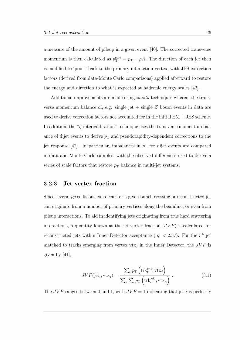
3.2.3 Jet vertex fraction
Since several pp collisions can occur for a given bunch crossing, a reconstructed jet
can originate from a number of primary vertices along the beamline, or even from
pileup interactions. To aid in identifying jets originating from true hard scattering
interactions, a quantity known as the jet vertex fraction (JV F ) is calculated for
reconstructed jets within Inner Detector acceptance (|η| < 2.37). For the ith jet
matched to tracks emerging from vertex vtxj in the Inner Detector, the JV F is
given by [41],
JV F (jeti, vtxj) =
∑
k pT
(
trkjetik , vtxj
)
∑
n
∑
l pT
(
trkjetil , vtxn
) . (3.1)
The JV F ranges between 0 and 1, with JV F = 1 indicating that jet i is perfectly
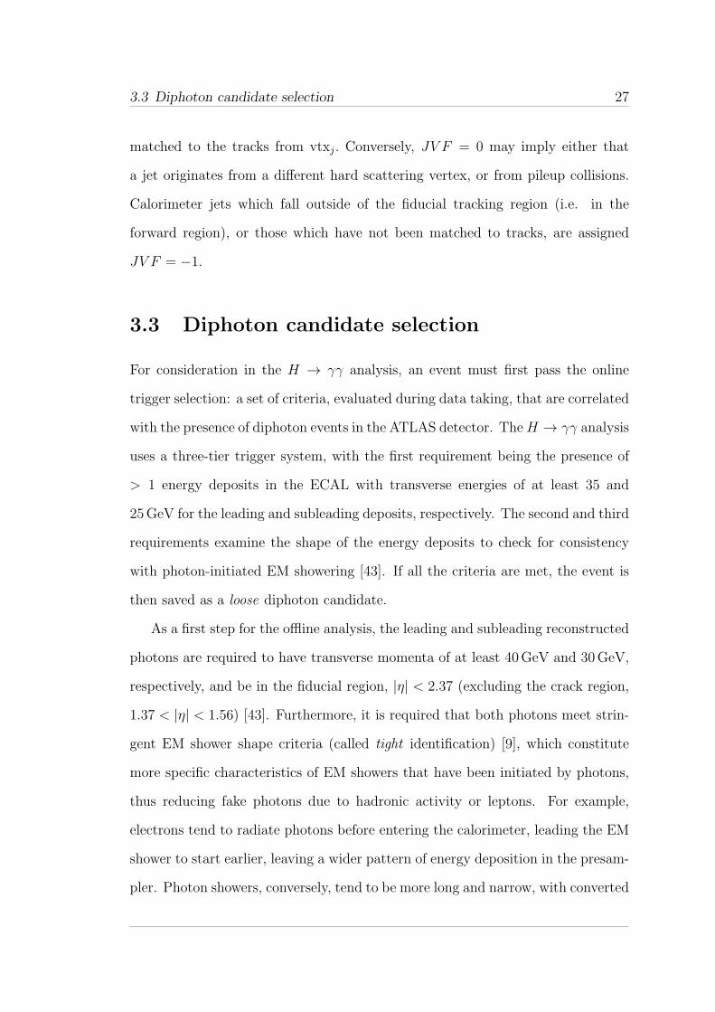
3.3 Diphoton candidate selection 27
matched to the tracks from vtxj. Conversely, JV F = 0 may imply either that
a jet originates from a different hard scattering vertex, or from pileup collisions.
Calorimeter jets which fall outside of the fiducial tracking region (i.e. in the
forward region), or those which have not been matched to tracks, are assigned
JV F = −1.
3.3 Diphoton candidate selection
For consideration in the H → γγ analysis, an event must first pass the online
trigger selection: a set of criteria, evaluated during data taking, that are correlated
with the presence of diphoton events in the ATLAS detector. TheH → γγ analysis
uses a three-tier trigger system, with the first requirement being the presence of
> 1 energy deposits in the ECAL with transverse energies of at least 35 and
25GeV for the leading and subleading deposits, respectively. The second and third
requirements examine the shape of the energy deposits to check for consistency
with photon-initiated EM showering [43]. If all the criteria are met, the event is
then saved as a loose diphoton candidate.
As a first step for the offline analysis, the leading and subleading reconstructed
photons are required to have transverse momenta of at least 40GeV and 30GeV,
respectively, and be in the fiducial region, |η| < 2.37 (excluding the crack region,
1.37 < |η| < 1.56) [43]. Furthermore, it is required that both photons meet strin-
gent EM shower shape criteria (called tight identification) [9], which constitute
more specific characteristics of EM showers that have been initiated by photons,
thus reducing fake photons due to hadronic activity or leptons. For example,
electrons tend to radiate photons before entering the calorimeter, leading the EM
shower to start earlier, leaving a wider pattern of energy deposition in the presam-
pler. Photon showers, conversely, tend to be more long and narrow, with converted
3.3 Diphoton candidate selection 28
photon shower shapes falling in-between in terms of shower width and length.
Beyond cuts on pT and |η|, photons are required to be well-isolated in both
the calorimeter, and Inner Detector (for single and double conversions). For the
calorimeter, isolation is defined in terms of ET, such that the sum of the transverse
energy of all topological clusters within ∆R < 0.4 of the photon must be less than
6GeV [43], excluding the energy deposits belonging to the photon itself. In the
case of single- or double-track conversions, the additional requirement on track
isolation is defined in terms of track pT, such that the scalar sum of the transverse
momenta of all tracks within ∆R < 0.2 must be less than 2.6GeV [43].
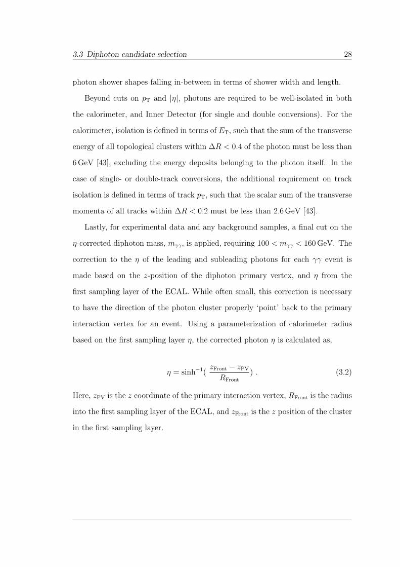
Lastly, for experimental data and any background samples, a final cut on the
η-corrected diphoton mass, mγγ, is applied, requiring 100 < mγγ < 160GeV. The
correction to the η of the leading and subleading photons for each γγ event is
made based on the z-position of the diphoton primary vertex, and η from the
first sampling layer of the ECAL. While often small, this correction is necessary
to have the direction of the photon cluster properly ‘point’ back to the primary
interaction vertex for an event. Using a parameterization of calorimeter radius
based on the first sampling layer η, the corrected photon η is calculated as,
η = sinh−1(zFront − zPVRFront
) . (3.2)
Here, zPV is the z coordinate of the primary interaction vertex, RFront is the radius
into the first sampling layer of the ECAL, and zFront is the z position of the cluster
in the first sampling layer.
3.4 Dijet candidate selection 29
3.4 Dijet candidate selection
Since the detection of any vector boson fusion event relies heavily on the proper
measurement of the outgoing quark jets, imposing quality cuts on reconstructed
jets is also necessary for this analysis. As a baseline, all reconstructed jets are
required to have a transverse momentum greater than 25GeV (30GeV) for |η| <
2.5 (2.5 < |η| < 4.5) to be considered. In addition, |JV F | > 0.25 is required
of all jets in the central region which are matched to tracks emerging from the
primary interaction vertex. Finally, in order to prevent the misidentification of
photons and electrons as hadronic jets and vice versa, a cut is placed on the
spatial separation of calorimeter objects, requiring ∆R > 0.4 between all physics
objects.2 Worth noting is that the η, φ values used in this cut are taken from
the EM scale jet, negating any changes in direction from applying jet energy scale
corrections. Once the selection is complete, the two highest pT jets are used for
further categorization.
3.5 Event categorization
Events passing initial diphoton selection are divided into a number of exclusive
categories meant to isolate events with photon, jet, and lepton properties char-
acteristic of vector boson fusion, associated production (V H), or gluon-gluon fu-
sion [43]. The categorization occurs in a hierarchical manner, with associated
production-enriched categories taking top precedence. These categories exploit
the presence of electrons or muons, low-mass dijet pairs, or missing transverse
energy to search for Higgsstrahlung-like H → γγ signal. Any diphoton + dijet
events failing the V H criteria are then considered for the secondary, VBF-enriched
2 Though not relevant to this analysis, quality cuts are also applied for electrons and muons,which are detailed in Ref. [16].
3.5 Event categorization 30
category. Any diphoton + dijet events that fail the VBF criteria, or events with
< 2 good jets, are then placed in an inclusive categorization based on pTt, photon
|η|, and the number of converted photons in the pair.
Figure 3.1: Explanatory diagram of pTt, the component of the diphoton transversemomentum ~pγγT transverse to the diphoton thrust axis t [44].
Note that pTt is the component of the diphoton transverse momentum ~pγγT trans-
verse to the diphoton thrust axis t (see Figure 3.1), with its magnitude defined
as [45, 46],
pTt ≡ |pTt| = |~pγγT × t|, where t = ~pγ1T − ~pγ2T|~pγ1T − ~pγ2T |
. (3.3)
The category relevant to this analysis is that which is enriched with VBF-like
events. In prior analyses, this category was defined entirely using rectangular cuts
on quantities sensitive to diphoton + dijet systems, like mjj, ∆ηjj, and ∆φγγjj.
However, for the most recent iteration of the H → γγ analysis, the VBF category
was split into two subcategories (high and low VBF-like), with the selection process
motivated entirely by multivariate analysis techniques – specifically, the usage of
boosted decision trees. Both the derivation of this new mode of categorization,
and a study of its efficacy, are detailed in Chapters 4 and 5.
Chapter 4
Introducing the VBF multivariate
analysis
4.1 Boosted decision trees
The boosted decision tree (BDT) method is a form of multivariate analysis offered
in the Toolkit for Multivariate Analysis (TMVA) package [47]. A boosted decision
tree uses multiple binary decision trees (as shown in Figure 4.1) to form a robust,
statistically stable classifier which discriminates signal from background events in
a data sample. Each constituent binary tree is built from a list of user-provided
discriminating variables, and trained using distinct, non-overlapping signal and
background samples. The function of each tree is to use a series of ‘yes/no’ deci-
sions to classify individual events as signal-like or background-like.
The result from each tree (the leaf node) is then combined via weighted aver-
age into a single discriminant, known as the BDT score [47]. Typically, this score
varies on [-1, +1], with background-like events assigned low (or negative) scores,
and signal-like events assigned highly positive scores. The ‘boosting’ aspect de-
rives from the fact that the weight of each tree is proportionate to its rate of
31
4.2 Signal and background modelling 33
ferentiate signal from background, and show no bias towards any value of the
quantity (or quantities) of interest in the analysis. The confluence of these two
elements will produce an optimized, robust BDT-based analysis.
4.2 Signal and background modelling
4.2.1 Signal modelling
The signal Monte Carlo samples used in the H → γγ analysis are typically gener-
ated using the Powheg package [29, 30], which simulates Higgs boson signal events
using exact NLO QCD matrix elements. The physical interactions that Powheg
generates are deemed parton-level, as they describe only the hardest emission
for a given process. All other higher-level processes (showering, parton split-
ting, gluon radiation, etc.) require the usage of a dedicated shower Monte Carlo
(SMC) program [29]. For this reason, the parton-level output is interfaced with
Pythia [35], an NLO generator that contains modules to simulate parton shower-
ing and hadronization, thus leading to truth-level information. Finally, this set of
truth-level particles is run through a full simulation of the ATLAS detector using
GEANT4 [49, 50], and reconstructed by the same offline ATLAS software used for
data reconstruction [51].
4.2.2 Background modelling
Background estimation techniques in the H → γγ analysis can originate both in
simulated data, as well as data-driven methods [19], owing to the large reducible
background from γj events. The data-driven methods typically form an estimate
based on the sideband data,1 or through the reversal of a cut from the diphoton cut
1 Diphoton event candidates with mγγ > 130GeV || mγγ < 120GeV.
4.2 Signal and background modelling 34
flow (as detailed in Section 3.3). Specifically, background samples can be created
from a reversal of the tight identification cuts (known as inverted ID samples), or
the calorimeter + track isolation cuts (known as inverted isolation).
Because any Higgs boson-like resonance will be directly observable from the
mγγ spectrum as a ‘bump’, one may also estimate the background distribution
by fitting an analytic function to the data region(s) where the resonance is not
observed. In particular, shape estimation for the γγ background is treated using an
exponential distribution or Bernstein polynomial, with the estimate derived using
a fit to the left and right signal region sidebands (defined as 100 < mγγ < 120
GeV and 130 < mγγ < 160 GeV, respectively) [34]. The ultimate goal of this
sideband fit is to allow an accurate estimate of the background in the signal region,
120 < mγγ < 130 GeV, which can be used to quantify the statistical significance
of any signal-like trend in the mγγ spectrum.
Additionally, several γγ, γj process Monte Carlo generators are available
within ATLAS for background estimation, which may simulate parton-level physics
processes (typically at NLO), secondary interactions (such as parton showering),
or perform both. In the H → γγ analysis, Sherpa [52, 53] is typically used for
background studies. Sherpa is an O (α2) generator that simulates both γγ (i.e.
Born, Box) and γj background processes. Hard scattering interactions are simu-
lated using a matrix-element generator, which are then interfaced with modules
that deal with initial- and final-state parton showering, multiple parton interac-
tions, parton hadronization, and hadronic decay [53].
4.2.3 Monte Carlo event weights
Most high-level Monte Carlo generators rely on approximate or fixed-order solu-
tions to the equations governing the hard scattering and showering interactions
4.3 Input sample selection 35
observed in particle accelerators. So, when combined with the various detector
effects and potential mismodelling of variables which are unaccounted for in full
detector-simulated Monte Carlo samples, there is potential for non-trivial disagree-
ment between experimental data and simulation.
One option to mitigate these differences is to assign data-driven weights, mod-
ifying the shapes of the Monte Carlo distributions to better match those observed
in data. Most notably, a pileup weight is applied for all Monte Carlo samples,
the function of which is to bring the distribution of the average bunch crossing
multiplicity (〈µ〉) in agreement between data and Monte Carlo distributions, to
account for variances in luminosity and pileup between data runs in ATLAS. A
reweighting based on the hard scatter z-vertex position is also applied, which
is used to correct the observed difference in z-vertex spread between data and
Monte Carlo samples. For ggF samples, an interference weight is also applied,
which accounts for destructive interference between the gg → γγ background and
the gg → H → γγ process [54, 55].
4.3 Input sample selection
4.3.1 Samples available for the multivariate analysis
Any data-driven aspects of the derivation and optimization of this BDT-based
analysis were based on (∼ 13.0 ± 3.6%) fb−1 of proton-proton collision data col-
lected at the LHC, recorded during 2012. The collisions occurred with a centre-
of-mass energy of√s = 8TeV, with the average number of primary vertices being
20.0 [56]. The standard diphoton trigger outlined in Section 3.3 was used in the
analysis, with the final trigger efficiency being > 99% for the entire data set. Fur-
thermore, for the purposes of this analysis, diphoton pairs were allowed to have a
4.3 Input sample selection 36
mass in the range 100 < mγγ < 170GeV.
Within this analysis, Monte Carlo samples were used to simulate both signal
and background processes. The signal Monte Carlo samples used in the multi-
variate analysis, corresponding to VBF H → γγ and ggF H → γγ processes,
were generated using Powheg + Pythia8 (as described in Section 4.2.1), with
mH = 125GeV. The background Monte Carlo samples in this analysis primarily
involved Sherpa γγ, γj events (see Section 4.2.2), wherein each event contained
a diphoton pair with mγγ > 80GeV, and up to three parton jets generated from
matrix elements. Sideband data samples were also available to use as background,
along with inverted ID and inverted isolation background data, as summarized in
Table 4.1.
4.3.2 Signal, background sample configuration
The first task in developing the BDT-based analysis was to select samples that
could model well the VBF H → γγ signal, as well as the diphoton and dijet
components of the background. Before any specific tests were made, a series of
ground rules about sample composition was decided on, in order to ensure the
most unbiased analysis possible:
• All training/testing samples must be orthogonal. In this analysis, the
requirement on sample orthogonality was two-fold. Firstly, it was required
that there be no overlapping events among the signal and background sam-
ples used to build and test the BDT, which would otherwise lead to poor
BDT training and ineffective signal event selection. Secondly, it was required
that the training and testing samples be orthogonal, in order to prevent the
introduction of biases in classifying potential VBF events.
4.3 Input sample selection 37
• All diphoton + dijet data samples must have the signal region
blinded. Any diphoton + dijet candidate data events with 120 < mγγ <
130GeV were excluded from the analysis, in order to limit any potential
biases on mγγ. Note that this blinding does not apply to background data,
or any Monte Carlo samples.
• Events in associated production-enriched categories must be ex-
cluded. In order to ensure that each sample attained the highest possible
purity of VBF-like events, any diphoton + dijet events in the V H-enriched
categories (see Section 3.5) were immediately vetoed from entering any train-
ing or testing sample.
With these rules established, it was possible to move on to select appropriate
signal and background samples for training the BDT.
4.3.3 Background training sample selection
The fact that the background for the H → γγ process encompasses pairs of real
and fake photons presents a unique challenge for selecting a proper background
sample. In order to successfully emulate the true diphoton background after event
selection, a sample must accurately model the γγ, γj, and jj components of the
background. To this end, a variety of background estimation methods were tested,
with the different types of models explained in Table 4.1.
The initial hope was to be able to use a data-driven estimation for training,
which would remove the need to individually model the different H → γγ back-
ground components. One option was the direct usage of a portion of the data
sidebands for training, with the other being the usage of inverted isolation or in-
verted ID background data. It was found that after diphoton + dijet selection,
V H category vetoes, and division into training/testing samples, the statistics of
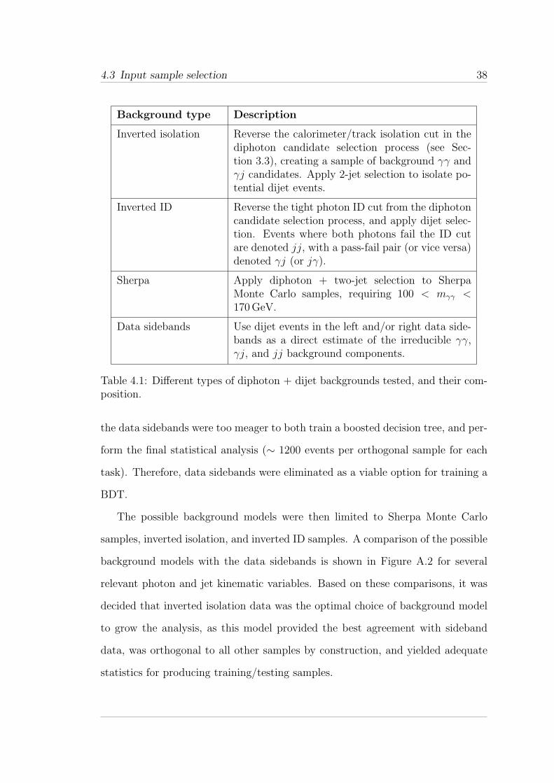
4.3 Input sample selection 38
Background type Description
Inverted isolation Reverse the calorimeter/track isolation cut in thediphoton candidate selection process (see Sec-tion 3.3), creating a sample of background γγ andγj candidates. Apply 2-jet selection to isolate po-tential dijet events.
Inverted ID Reverse the tight photon ID cut from the diphotoncandidate selection process, and apply dijet selec-tion. Events where both photons fail the ID cutare denoted jj, with a pass-fail pair (or vice versa)denoted γj (or jγ).
Sherpa Apply diphoton + two-jet selection to SherpaMonte Carlo samples, requiring 100 < mγγ <170GeV.
Data sidebands Use dijet events in the left and/or right data side-bands as a direct estimate of the irreducible γγ,γj, and jj background components.
Table 4.1: Different types of diphoton + dijet backgrounds tested, and their com-position.
the data sidebands were too meager to both train a boosted decision tree, and per-
form the final statistical analysis (∼ 1200 events per orthogonal sample for each
task). Therefore, data sidebands were eliminated as a viable option for training a
BDT.
The possible background models were then limited to Sherpa Monte Carlo
samples, inverted isolation, and inverted ID samples. A comparison of the possible
background models with the data sidebands is shown in Figure A.2 for several
relevant photon and jet kinematic variables. Based on these comparisons, it was
decided that inverted isolation data was the optimal choice of background model
to grow the analysis, as this model provided the best agreement with sideband
data, was orthogonal to all other samples by construction, and yielded adequate
statistics for producing training/testing samples.
4.4 Input variable selection 39
4.4 Input variable selection
4.4.1 Deriving a list of discriminating variables
Beyond selecting proper training samples, a primary concern in the development
of any BDT-based analysis is the choice of discriminating variables that agree well
with theoretical predictions of the process under study, provide good discrimina-
tion between the desired signal and unwanted processes, and also sidestep any
undesirable biases. To this end, all potential classifiers were required to fulfill a
series of preliminary criteria before training to ensure a robust, unbiased analysis.
First, each variable was required to have little to no correlation to the diphoton
mass, mγγ. This relation was determined through the calculation of a linear corre-
lation coefficient (LCC) between mγγ and a given variable, with the scale ranging
from −100% (completely anticorrelated) to +100% (completely correlated). This
criterion was of singular importance. If it was not met, the selection process would
be immediately biased towards events with mγγ ∼ 125GeV.
Second, for the remaining variables uncorrelated to mγγ, each quantity was to
be ranked according to its signal/background discriminating power, as given by
the separation 〈S2〉, and the variable importance. The former quantity is entirely
shape-based, and is calculated as [47],
⟨
S2⟩
=1
2
Nbins∑
i=1
(si − bi)2
si + bi, (4.1)
where s and b are signal and background probability density functions (PDFs)
for a given classifier. The variable importance, by contrast, is a BDT-specific
quantity, and quantifies how frequently a variable is used to split nodes (i.e. make
decisions). It is computed for a given variable as the frequency of its use in node
splitting, weighted by both the number of events in each node, and the separation
4.4 Input variable selection 40
gain-squared it achieved [47]. If a given input variable demonstrated both high
separating power in terms of 〈S2〉 and importance, then it was considered for
further usage in training the BDT.
A tertiary criterion for each potential classifier was a low correlation (expressed
in terms of LCCs) to other candidate variables. Unlike other multivariate anal-
ysis techniques such as neural networks, uncorrelated input variables are not a
fundamental requirement for BDTs [47], as the presence of two highly correlated
classifiers results only in suboptimal signal discrimination, rather than a bias in
the distributions of the selected events.
With a formal set of selection criteria established, the variable selection process
began by training with an initially large list of variables, which would highlight the
classifiers that were used most frequently and/or effectively to separate signal from
background. The initial list of classifiers was composed of 23 variables, spanning
a range of single jet, single photon, and dijet/diphoton quantities:
pT(jet1,2,3), ηjet1,2,3, φjet1,2,3, JV Fjet1,2,3
ηZeppjet3 , ηZeppγγ , min(∆Rjγ), mjj, ∆ηjj
∆φ(jj), ∆φγγjj, ∆pT(jj), ∆pT(γγ), pTγγjj, pTt
Note: Definitions of these variables are found in Table A.1.
The initial BDT training was then performed using VBF H → γγ Monte Carlo
samples with mH = 125GeV as a signal training sample, and 2012 inverted iso-
lation data as the background training sample. Each sample was split up into
training/testing subsets according to event number, as follows:
Event number mod 2 =
0 → Testing
1 → Training
(4.2)
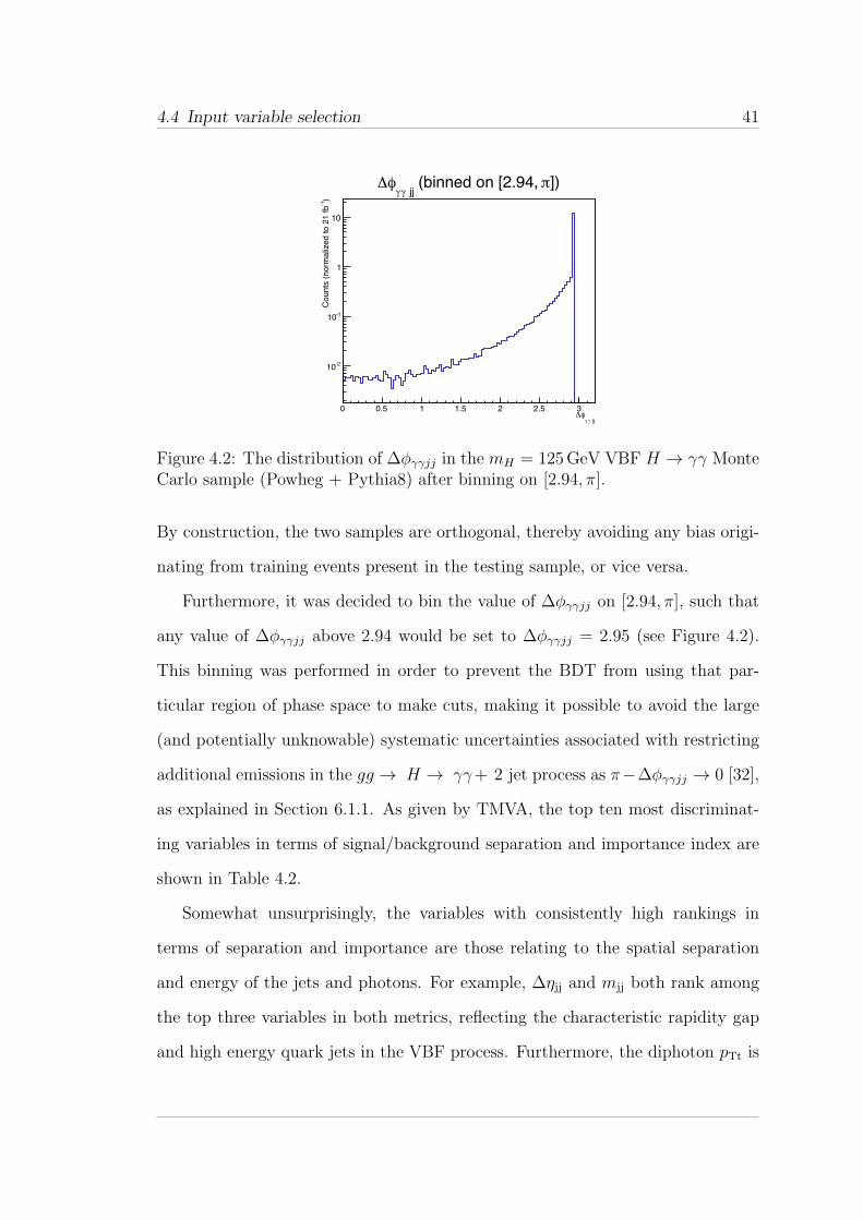
4.4 Input variable selection 41
jj!!"#
0 0.5 1 1.5 2 2.5 3
)-1
Counts
(norm
aliz
ed t
o 2
1 f
b
-210
-110
1
10
])$ (binned on [2.94, jj!!
"#
Figure 4.2: The distribution of ∆φγγjj in the mH = 125GeV VBF H → γγ MonteCarlo sample (Powheg + Pythia8) after binning on [2.94, π].
By construction, the two samples are orthogonal, thereby avoiding any bias origi-
nating from training events present in the testing sample, or vice versa.
Furthermore, it was decided to bin the value of ∆φγγjj on [2.94, π], such that
any value of ∆φγγjj above 2.94 would be set to ∆φγγjj = 2.95 (see Figure 4.2).
This binning was performed in order to prevent the BDT from using that par-
ticular region of phase space to make cuts, making it possible to avoid the large
(and potentially unknowable) systematic uncertainties associated with restricting
additional emissions in the gg → H → γγ+ 2 jet process as π−∆φγγjj → 0 [32],
as explained in Section 6.1.1. As given by TMVA, the top ten most discriminat-
ing variables in terms of signal/background separation and importance index are
shown in Table 4.2.
Somewhat unsurprisingly, the variables with consistently high rankings in
terms of separation and importance are those relating to the spatial separation
and energy of the jets and photons. For example, ∆ηjj and mjj both rank among
the top three variables in both metrics, reflecting the characteristic rapidity gap
and high energy quark jets in the VBF process. Furthermore, the diphoton pTt is
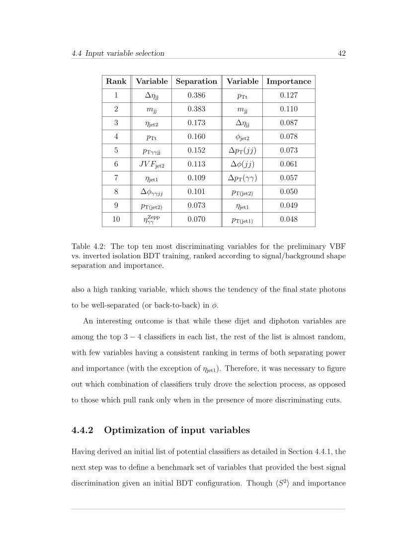
4.4 Input variable selection 42
Rank Variable Separation Variable Importance
1 ∆ηjj 0.386 pTt 0.127
2 mjj 0.383 mjj 0.110
3 ηjet2 0.173 ∆ηjj 0.087
4 pTt 0.160 φjet2 0.078
5 pTγγjj 0.152 ∆pT(jj) 0.073
6 JV Fjet2 0.113 ∆φ(jj) 0.061
7 ηjet1 0.109 ∆pT(γγ) 0.057
8 ∆φγγjj 0.101 pT(jet2) 0.050
9 pT(jet2) 0.073 ηjet1 0.049
10 ηZeppγγ 0.070 pT(jet1) 0.048
Table 4.2: The top ten most discriminating variables for the preliminary VBFvs. inverted isolation BDT training, ranked according to signal/background shapeseparation and importance.
also a high ranking variable, which shows the tendency of the final state photons
to be well-separated (or back-to-back) in φ.
An interesting outcome is that while these dijet and diphoton variables are
among the top 3 − 4 classifiers in each list, the rest of the list is almost random,
with few variables having a consistent ranking in terms of both separating power
and importance (with the exception of ηjet1). Therefore, it was necessary to figure
out which combination of classifiers truly drove the selection process, as opposed
to those which pull rank only when in the presence of more discriminating cuts.
4.4.2 Optimization of input variables
Having derived an initial list of potential classifiers as detailed in Section 4.4.1, the
next step was to define a benchmark set of variables that provided the best signal
discrimination given an initial BDT configuration. Though 〈S2〉 and importance
4.4 Input variable selection 43
calculations give an indication of how a variable performs in identifying signal and
background in isolation, it is insufficient to judge a set of classifiers based on these
separation criteria alone. In particular, because the final analysis is defined by
the search for a resonance in the diphoton mass spectrum, it is more relevant and
intuitive to use a metric that has a direct relation to the probability of particle
discovery. For this reason, it was chosen to evaluate the list of benchmark variables
as the set of classifiers optimizing the approximate VBF significance for s≪ b,
S ≈ sVBF√
sVBF + sggF + b+∑
(syst. uncert.)2, (4.3)
where sVBF, sggF, and b are integrals of the mγγ distributions of the VBF and ggF
H → γγ signal Monte Carlo and background samples (respectively) over a given
mass range. Here,∑
(syst. uncert.)2 is the sum in quadrature of the different
systematic uncertainties of the analysis (see Chapter 6 for details). This term
is unique to the multivariate analysis, and serves as a ‘penalty’ for the choice of
variables with high associated theoretical and/or experimental uncertainties.
Two forms of the approximate significance were calculated, based on different
mγγ regions. The window significance was defined using integrals of the signal
and background distributions on [123, 127]GeV, while the shape significance was
obtained using integrals on the entire mass range. Owing to the narrow width of
the Higgs boson resonance in the VBF signal Monte Carlo sample, the variable
set maximizing shape significance should also maximize the window significance.
With a metric for judging performance determined, the following approach was
taken to derive a benchmark list of variables:
1. Based on the results of Section 4.4.1, a list of 8− 10 variables was created,
with which a new training was performed using VBF H → γγ signal Monte
Carlo and inverted isolation background samples. Classifiers for this training
4.4 Input variable selection 44
were required to have high separating power, and be frequently/effectively
used within the initial BDT.
2. BDTs were trained using every permutation of k variables in the n-variable
list (where 2 ≤ k ≤ n), with each trained BDT applied to each testing
sample (constituting VBF, ggF signal Monte Carlo samples, and sideband
data) separately. In total, for each k variables chosen,(
nk
)
BDT trainings
were performed.
3. For each permutation, using the resultant BDT score distributions for each
sample, a scan was made over the range of possible cuts on the discrimi-
nant. At each step of the scan, shape and window significance calculations
were performed. The combination of variables maximizing the approximate
significance values was taken to be the benchmark.
Of particular note is that the amount of VBF signal rejected by each permuta-
tion of variables and BDT score cut was also considered during the optimization
process, with the signal rejection obtained by translating the BDT score distribu-
tion to a flat distribution of 5% VBF rejection quantiles.2 That is to say, instead
of placing a cut on the BDT score itself by requiring BDT score > X, the nth cut
is more aptly described as requiring,
BDT score > X ′, such that
∫ X′
−1
dNVBF
dXdX = n× 0.05NVBF, where n ∈ [0, 20].
The shape and window significance values for the cases of BDT score > X ′ and
BDT score < X ′ were added in quadrature to form the final significance, although
the contribution from the latter case is heavily suppressed by background, such
2 Scanning over the range of BDT scores to produce a cut should yield the same optimalsignificance, hence why we don’t need or use the BDT score directly.
4.4 Input variable selection 45
that Sn ≈ S(BDT score > X ′). Ultimately, it was decided to test two different
sets of variables, with each having a mixture of single jet, dijet/diphoton, and
dijet + diphoton system quantities:
Selection A (10 total)
ηjet1, ηjet2, mjj,
∆ηjj, ∆φγγjj, pTt,
pTγγjj, ∆pT(jj),
∆φ(jj), ∆pT(γγ),
Selection B (8 total)
ηjet1, ηjet2
mjj, ∆ηjj,
∆φγγjj, pTt,
ηZeppγγ , min(∆Rjγ)
4.4.3 Final list of input variables
After comparing the shape and window VBF significance values for each permu-
tation of variables, as summarized in Tables 4.3 and 4.4, it was found that the
following six variables consistently performed the best at discriminating signal
from background:
mjj, ∆ηjj, ∆φγγjj, ηjet1, ηjet2, pTt
Each of these variables relates directly to the spatial separation of either the
dijet or diphoton systems. In particular, as shown in Table 4.3, when restricted
to selecting 2 − 4 variables, the dijet mass (mjj) and diphoton thrust pT (pTt)
are continuously the best variables for discriminating VBF H → γγ signal from
background. Furthermore, these results reinforce the hierarchy of variables shown
in Table 4.2, which also point to mjj and pTt as being highly discriminating both
in terms of shape separation and importance.
One interesting outcome is the discriminating power of ∆φγγjj, which initially
did not rank very highly in terms of separating power/importance on its own.
However, when used in confluence with several other variables, this dijet + dipho-
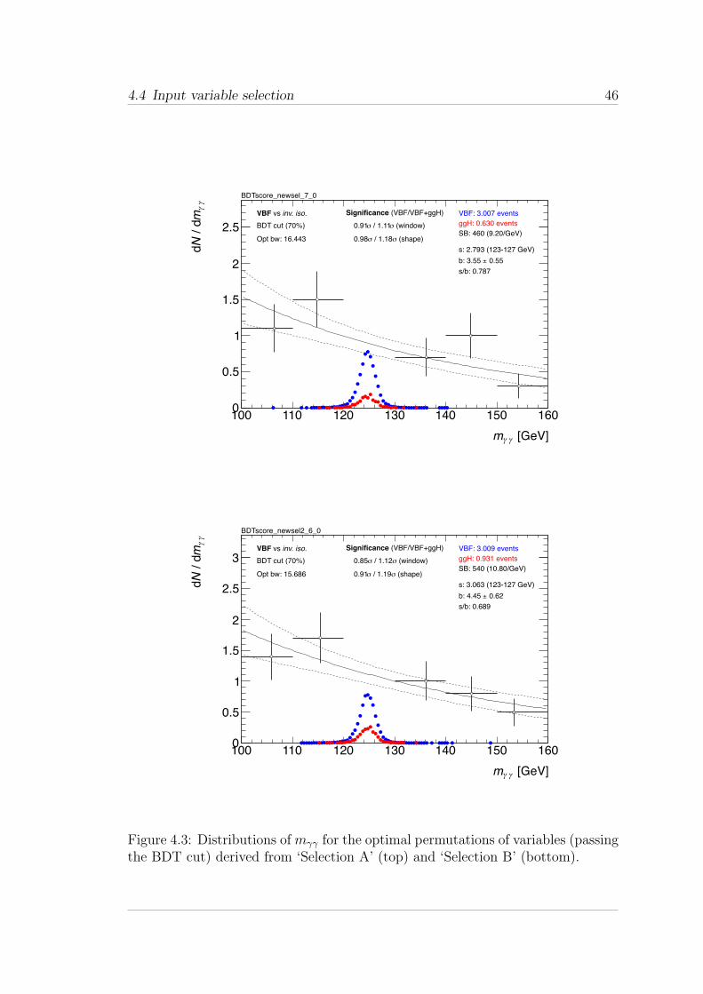
4.4 Input variable selection 46
[GeV]!!m
100 110 120 130 140 150 160
!!
m /
dN
d
0
0.5
1
1.5
2
2.5
VBF: 3.007 events
ggH: 0.630 events
SB: 460 (9.20/GeV)
s: 2.793 (123-127 GeV)
0.55±b: 3.55
s/b: 0.787
Opt bw: 16.443
(VBF/VBF+ggH)Significance
(window)" / 1.11"0.91
(shape)" / 1.18"0.98
inv. iso. vs VBF
BDTscore_newsel_7_0
BDT cut (70%)
[GeV]!!m
100 110 120 130 140 150 160
!!
m /
dN
d
0
0.5
1
1.5
2
2.5
3VBF: 3.009 events
ggH: 0.931 events
SB: 540 (10.80/GeV)
s: 3.063 (123-127 GeV)
0.62±b: 4.45
s/b: 0.689
Opt bw: 15.686
(VBF/VBF+ggH)Significance
(window)" / 1.12"0.85
(shape)" / 1.19"0.91
inv. iso. vs VBF
BDTscore_newsel2_6_0
BDT cut (70%)
Figure 4.3: Distributions ofmγγ for the optimal permutations of variables (passingthe BDT cut) derived from ‘Selection A’ (top) and ‘Selection B’ (bottom).
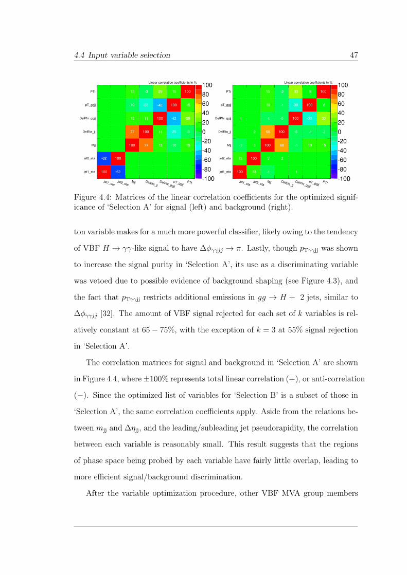
4.4 Input variable selection 47
-100
-80
-60
-40
-20
0
20
40
60
80
100
jet1_etajet2_eta
Mjj DelEta_jj
DelPhi_ggjj
pT_ggjjPTt
jet1_eta
jet2_eta
Mjj
DelEta_jj
DelPhi_ggjj
pT_ggjj
PTt
100 -62
-62 100
100 77 13 -10 15
77 100 11 -25 -3
13 11 100 -42 29
-10 -25 -42 100 15
15 -3 29 15 100
Linear correlation coefficients in %
-100
-80
-60
-40
-20
0
20
40
60
80
100
jet1_etajet2_eta
Mjj DelEta_jj
DelPhi_ggjj
pT_ggjjPTt
jet1_eta
jet2_eta
Mjj
DelEta_jj
DelPhi_ggjj
pT_ggjj
PTt
100 13 -1 1
13 100 3 2
-1 3 100 68 -1 19 15
2 68 100 -5 -1 -2
1 -1 -5 100 -30 33
19 -1 -30 100 8
15 -2 33 8 100
Linear correlation coefficients in %
0 0
Figure 4.4: Matrices of the linear correlation coefficients for the optimized signif-icance of ‘Selection A’ for signal (left) and background (right).
ton variable makes for a much more powerful classifier, likely owing to the tendency
of VBF H → γγ-like signal to have ∆φγγjj → π. Lastly, though pTγγjj was shown
to increase the signal purity in ‘Selection A’, its use as a discriminating variable
was vetoed due to possible evidence of background shaping (see Figure 4.3), and
the fact that pTγγjj restricts additional emissions in gg → H + 2 jets, similar to
∆φγγjj [32]. The amount of VBF signal rejected for each set of k variables is rel-
atively constant at 65− 75%, with the exception of k = 3 at 55% signal rejection
in ‘Selection A’.
The correlation matrices for signal and background in ‘Selection A’ are shown
in Figure 4.4, where±100% represents total linear correlation (+), or anti-correlation
(−). Since the optimized list of variables for ‘Selection B’ is a subset of those in
‘Selection A’, the same correlation coefficients apply. Aside from the relations be-
tween mjj and ∆ηjj, and the leading/subleading jet pseudorapidity, the correlation
between each variable is reasonably small. This result suggests that the regions
of phase space being probed by each variable have fairly little overlap, leading to
more efficient signal/background discrimination.
After the variable optimization procedure, other VBF MVA group members
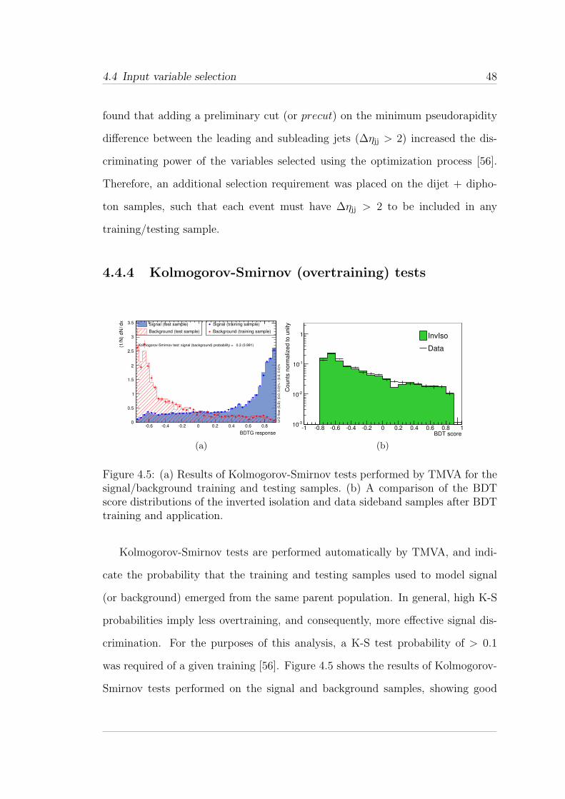
4.4 Input variable selection 48
found that adding a preliminary cut (or precut) on the minimum pseudorapidity
difference between the leading and subleading jets (∆ηjj > 2) increased the dis-
criminating power of the variables selected using the optimization process [56].
Therefore, an additional selection requirement was placed on the dijet + dipho-
ton samples, such that each event must have ∆ηjj > 2 to be included in any
training/testing sample.
4.4.4 Kolmogorov-Smirnov (overtraining) tests
BDTG response
-0.6 -0.4 -0.2 0 0.2 0.4 0.6 0.8
dx
/ (1
/N)
dN
0
0.5
1
1.5
2
2.5
3
3.5 Signal (test sample)
Background (test sample)
Signal (training sample)
Background (training sample)
Kolmogorov-Smirnov test: signal (background) probability = 0.3 (0.991)
U/O
-flo
w (
S,B
): (
0.0
, 0
.0)%
/ (
0.0
, 0
.0)%
(a)
BDT score-1 -0.8 -0.6 -0.4 -0.2 0 0.2 0.4 0.6 0.8 1
Co
un
ts n
orm
aliz
ed
to
un
ity
-310
-210
-110
1 InvIso
Data
(b)
Figure 4.5: (a) Results of Kolmogorov-Smirnov tests performed by TMVA for thesignal/background training and testing samples. (b) A comparison of the BDTscore distributions of the inverted isolation and data sideband samples after BDTtraining and application.
Kolmogorov-Smirnov tests are performed automatically by TMVA, and indi-
cate the probability that the training and testing samples used to model signal
(or background) emerged from the same parent population. In general, high K-S
probabilities imply less overtraining, and consequently, more effective signal dis-
crimination. For the purposes of this analysis, a K-S test probability of > 0.1
was required of a given training [56]. Figure 4.5 shows the results of Kolmogorov-
Smirnov tests performed on the signal and background samples, showing good
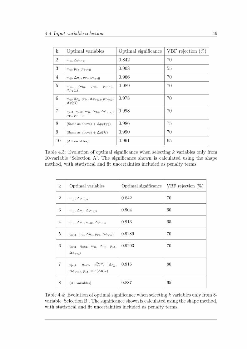
4.4 Input variable selection 49
k Optimal variables Optimal significance VBF rejection (%)
2 mjj, ∆φγγjj 0.842 70
3 mjj, pTt, pTγγjj 0.908 55
4 mjj, ∆ηjj, pTt, pTγγjj 0.966 70
5 mjj, ∆ηjj, pTt, pTγγjj,∆pT(jj)
0.989 70
6 mjj, ∆ηjj, pTt, ∆φγγjj , pTγγjj,∆φ(jj)
0.978 70
7 ηjet1, ηjet2, mjj, ∆ηjj, ∆φγγjj ,pTt, pTγγjj
0.998 70
8 (Same as above) + ∆pT(γγ) 0.986 75
9 (Same as above) + ∆φ(jj) 0.990 70
10 (All variables) 0.961 65
Table 4.3: Evolution of optimal significance when selecting k variables only from10-variable ‘Selection A’. The significance shown is calculated using the shapemethod, with statistical and fit uncertainties included as penalty terms.
k Optimal variables Optimal significance VBF rejection (%)
2 mjj, ∆φγγjj 0.842 70
3 mjj, ∆ηjj, ∆φγγjj 0.904 60
4 mjj, ∆ηjj, ηjet2, ∆φγγjj 0.913 65
5 ηjet1, mjj, ∆ηjj, pTt, ∆φγγjj 0.9289 70
6 ηjet1, ηjet2, mjj, ∆ηjj, pTt,
∆φγγjj
0.9293 70
7 ηjet1, ηjet2, ηZeppγγ , ∆ηjj,
∆φγγjj , pTt, min(∆Rjγ)
0.915 80
8 (All variables) 0.887 65
Table 4.4: Evolution of optimal significance when selecting k variables only from 8-variable ‘Selection B’. The significance shown is calculated using the shape method,with statistical and fit uncertainties included as penalty terms.
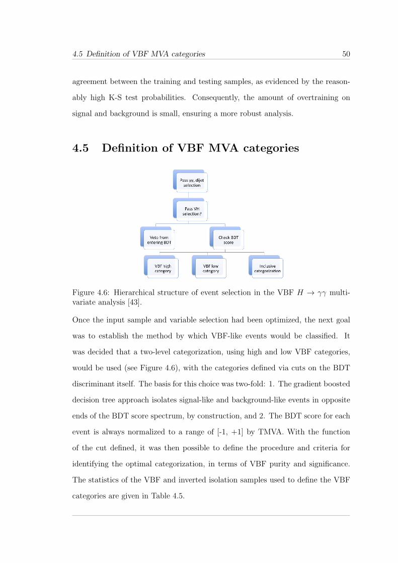
4.5 Definition of VBF MVA categories 50
agreement between the training and testing samples, as evidenced by the reason-
ably high K-S test probabilities. Consequently, the amount of overtraining on
signal and background is small, ensuring a more robust analysis.
4.5 Definition of VBF MVA categories
Figure 4.6: Hierarchical structure of event selection in the VBF H → γγ multi-variate analysis [43].
Once the input sample and variable selection had been optimized, the next goal
was to establish the method by which VBF-like events would be classified. It
was decided that a two-level categorization, using high and low VBF categories,
would be used (see Figure 4.6), with the categories defined via cuts on the BDT
discriminant itself. The basis for this choice was two-fold: 1. The gradient boosted
decision tree approach isolates signal-like and background-like events in opposite
ends of the BDT score spectrum, by construction, and 2. The BDT score for each
event is always normalized to a range of [-1, +1] by TMVA. With the function
of the cut defined, it was then possible to define the procedure and criteria for
identifying the optimal categorization, in terms of VBF purity and significance.
The statistics of the VBF and inverted isolation samples used to define the VBF
categories are given in Table 4.5.
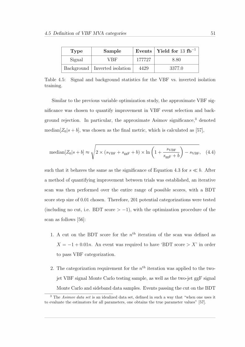
4.5 Definition of VBF MVA categories 51
Type Sample Events Yield for 13 fb−1
Signal VBF 177727 8.80
Background Inverted isolation 4429 3377.0
Table 4.5: Signal and background statistics for the VBF vs. inverted isolationtraining.
Similar to the previous variable optimization study, the approximate VBF sig-
nificance was chosen to quantify improvement in VBF event selection and back-
ground rejection. In particular, the approximate Asimov significance,3 denoted
median[Z0|s+ b], was chosen as the final metric, which is calculated as [57],
median[Z0|s+ b] ≈√
2× (sVBF + sggF + b)× ln
(
1 +sVBF
sggF + b
)
− sVBF, (4.4)
such that it behaves the same as the significance of Equation 4.3 for s≪ b. After
a method of quantifying improvement between trials was established, an iterative
scan was then performed over the entire range of possible scores, with a BDT
score step size of 0.01 chosen. Therefore, 201 potential categorizations were tested
(including no cut, i.e. BDT score > −1), with the optimization procedure of the
scan as follows [56]:
1. A cut on the BDT score for the nth iteration of the scan was defined as
X = −1 + 0.01n. An event was required to have ‘BDT score > X’ in order
to pass VBF categorization.
2. The categorization requirement for the nth iteration was applied to the two-
jet VBF signal Monte Carlo testing sample, as well as the two-jet ggF signal
Monte Carlo and sideband data samples. Events passing the cut on the BDT
3 The Asimov data set is an idealized data set, defined in such a way that “when one uses itto evaluate the estimators for all parameters, one obtains the true parameter values” [57].
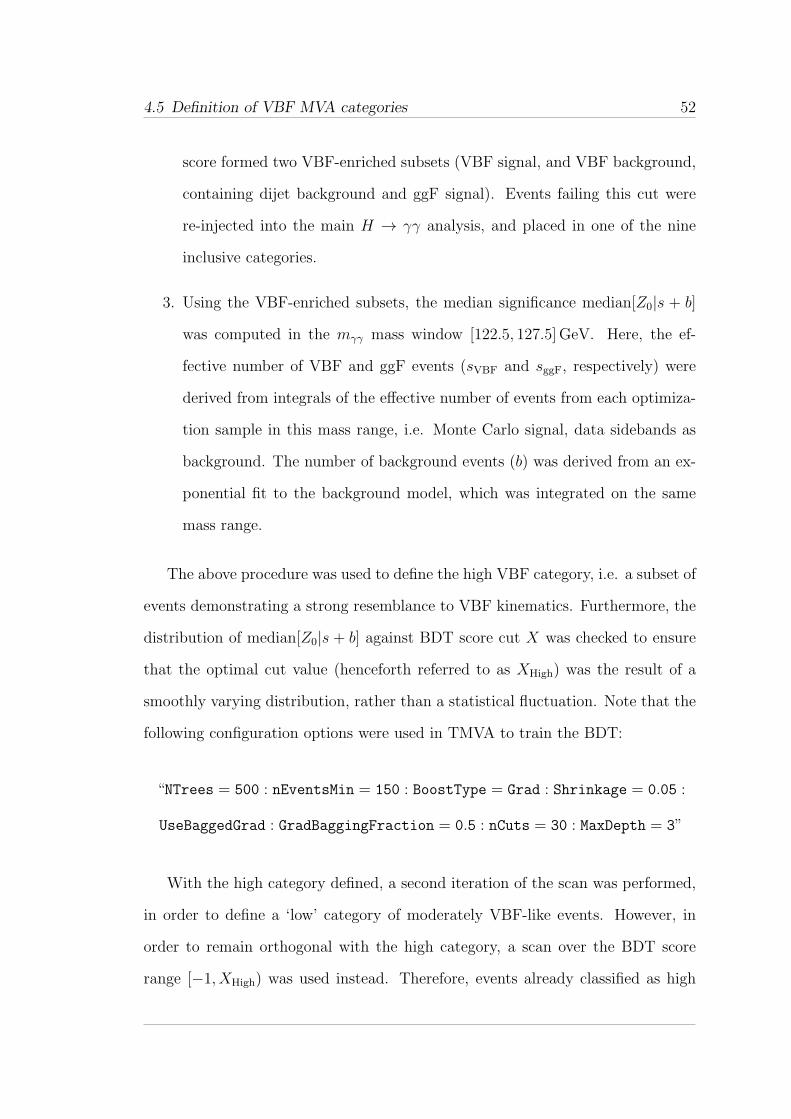
4.5 Definition of VBF MVA categories 52
score formed two VBF-enriched subsets (VBF signal, and VBF background,
containing dijet background and ggF signal). Events failing this cut were
re-injected into the main H → γγ analysis, and placed in one of the nine
inclusive categories.
3. Using the VBF-enriched subsets, the median significance median[Z0|s + b]
was computed in the mγγ mass window [122.5, 127.5]GeV. Here, the ef-
fective number of VBF and ggF events (sVBF and sggF, respectively) were
derived from integrals of the effective number of events from each optimiza-
tion sample in this mass range, i.e. Monte Carlo signal, data sidebands as
background. The number of background events (b) was derived from an ex-
ponential fit to the background model, which was integrated on the same
mass range.
The above procedure was used to define the high VBF category, i.e. a subset of
events demonstrating a strong resemblance to VBF kinematics. Furthermore, the
distribution of median[Z0|s + b] against BDT score cut X was checked to ensure
that the optimal cut value (henceforth referred to as XHigh) was the result of a
smoothly varying distribution, rather than a statistical fluctuation. Note that the
following configuration options were used in TMVA to train the BDT:
“NTrees = 500 : nEventsMin = 150 : BoostType = Grad : Shrinkage = 0.05 :
UseBaggedGrad : GradBaggingFraction = 0.5 : nCuts = 30 : MaxDepth = 3”
With the high category defined, a second iteration of the scan was performed,
in order to define a ‘low’ category of moderately VBF-like events. However, in
order to remain orthogonal with the high category, a scan over the BDT score
range [−1, XHigh) was used instead. Therefore, events already classified as high
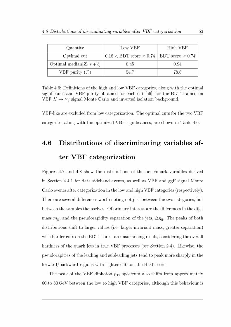
4.6 Distributions of discriminating variables after VBF categorization 53
Quantity Low VBF High VBF
Optimal cut 0.18 < BDT score < 0.74 BDT score ≥ 0.74
Optimal median[Z0|s+ b] 0.45 0.94
VBF purity (%) 54.7 78.6
Table 4.6: Definitions of the high and low VBF categories, along with the optimalsignificance and VBF purity obtained for each cut [56], for the BDT trained onVBF H → γγ signal Monte Carlo and inverted isolation background.
VBF-like are excluded from low categorization. The optimal cuts for the two VBF
categories, along with the optimized VBF significances, are shown in Table 4.6.
4.6 Distributions of discriminating variables af-
ter VBF categorization
Figures 4.7 and 4.8 show the distributions of the benchmark variables derived
in Section 4.4.1 for data sideband events, as well as VBF and ggF signal Monte
Carlo events after categorization in the low and high VBF categories (respectively).
There are several differences worth noting not just between the two categories, but
between the samples themselves. Of primary interest are the differences in the dijet
mass mjj, and the pseudorapidity separation of the jets, ∆ηjj. The peaks of both
distributions shift to larger values (i.e. larger invariant mass, greater separation)
with harder cuts on the BDT score – an unsurprising result, considering the overall
hardness of the quark jets in true VBF processes (see Section 2.4). Likewise, the
pseudorapities of the leading and subleading jets tend to peak more sharply in the
forward/backward regions with tighter cuts on the BDT score.
The peak of the VBF diphoton pTt spectrum also shifts from approximately
60 to 80GeV between the low to high VBF categories, although this behaviour is
4.6 Distributions of discriminating variables after VBF categorization 54
not unique to VBF.4 However, this shift is indicative that more central diphoton
pairs are being isolated by these cuts, which is reflective of the low-momentum
Higgs boson produced in the VBF process. Lastly, ∆φγγjj also tends towards
higher values between the low and high categories, indicating a momentum balance
between the dijet and diphoton systems, as expected of the tree-level VBF H →
γγ process.
Figures 4.9 and 4.10 show comparisons of the inverted isolation and data side-
band events in the low and high VBF categories, respectively. While agreement
in the former category is fairly good between the two samples, the low statistics
of the samples after the tighter BDT score cut lead to disagreement in the shapes
of some of the benchmark variables (e.g. ηjet2). Otherwise, the two samples gen-
erally agree within statistical errors, so it can be said that the inverted isolation
background is a fair descriptor of the diphoton background.
4 This behaviour is also observed in the ggF pTt spectrum.
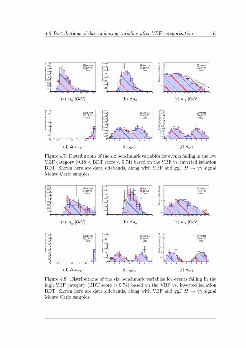
4.6 Distributions of discriminating variables after VBF categorization 55
0 200 400 600 800 1000 1200 1400
Counts
norm
aliz
ed to u
nity
0
0.02
0.04
0.06
0.08
0.1
0.12
0.14
0.16
0.18
0.2
VBF125
ggF125
Data
(a) mjj [GeV]
0 1 2 3 4 5 6 7 8 9
Counts
norm
aliz
ed to u
nity
0
0.02
0.04
0.06
0.08
0.1
0.12
0.14
0.16
VBF125
ggF125
Data
(b) ∆ηjj
0 20 40 60 80 100 120 140 160 180 200 220
Counts
norm
aliz
ed to u
nity
-210
-110
1
VBF125
ggF125
Data
(c) pTt [GeV]
0 0.5 1 1.5 2 2.5 3
Counts
norm
aliz
ed to u
nity
0
0.2
0.4
0.6
0.8
1
1.2VBF125
ggF125
Data
(d) ∆φγγjj
-4 -3 -2 -1 0 1 2 3 4
Counts
norm
aliz
ed to u
nity
0
0.02
0.04
0.06
0.08
0.1
0.12
0.14
0.16
0.18
0.2
VBF125
ggF125
Data
(e) ηjet1
-4 -3 -2 -1 0 1 2 3 4
Counts
norm
aliz
ed to u
nity
0
0.02
0.04
0.06
0.08
0.1
0.12
0.14
0.16
0.18
0.2
0.22
VBF125
ggF125
Data
(f) ηjet2
Figure 4.7: Distributions of the six benchmark variables for events falling in the lowVBF category (0.18 < BDT score < 0.74) based on the VBF vs. inverted isolationBDT. Shown here are data sidebands, along with VBF and ggF H → γγ signalMonte Carlo samples.
0 200 400 600 800 1000 1200 1400
Counts
norm
aliz
ed to u
nity
0
0.02
0.04
0.06
0.08
0.1
0.12
0.14
0.16
0.18
VBF125
ggF125
Data
(a) mjj [GeV]
0 1 2 3 4 5 6 7 8 9
Counts
norm
aliz
ed to u
nity
0
0.02
0.04
0.06
0.08
0.1
0.12
0.14
VBF125
ggF125
Data
(b) ∆ηjj
0 20 40 60 80 100 120 140 160 180 200 220
Counts
norm
aliz
ed to u
nity
-210
-110
1 VBF125
ggF125
Data
(c) pTt [GeV]
0 0.5 1 1.5 2 2.5 3
Counts
norm
aliz
ed to u
nity
0
0.2
0.4
0.6
0.8
1
1.2
1.4
1.6
1.8 VBF125
ggF125
Data
(d) ∆φγγjj
-4 -3 -2 -1 0 1 2 3 4
Counts
norm
aliz
ed to u
nity
0
0.05
0.1
0.15
0.2
0.25
0.3VBF125
ggF125
Data
(e) ηjet1
-4 -3 -2 -1 0 1 2 3 4
Counts
norm
aliz
ed to u
nity
0
0.05
0.1
0.15
0.2
0.25VBF125
ggF125
Data
(f) ηjet2
Figure 4.8: Distributions of the six benchmark variables for events falling in thehigh VBF category (BDT score > 0.74) based on the VBF vs. inverted isolationBDT. Shown here are data sidebands, along with VBF and ggF H → γγ signalMonte Carlo samples.
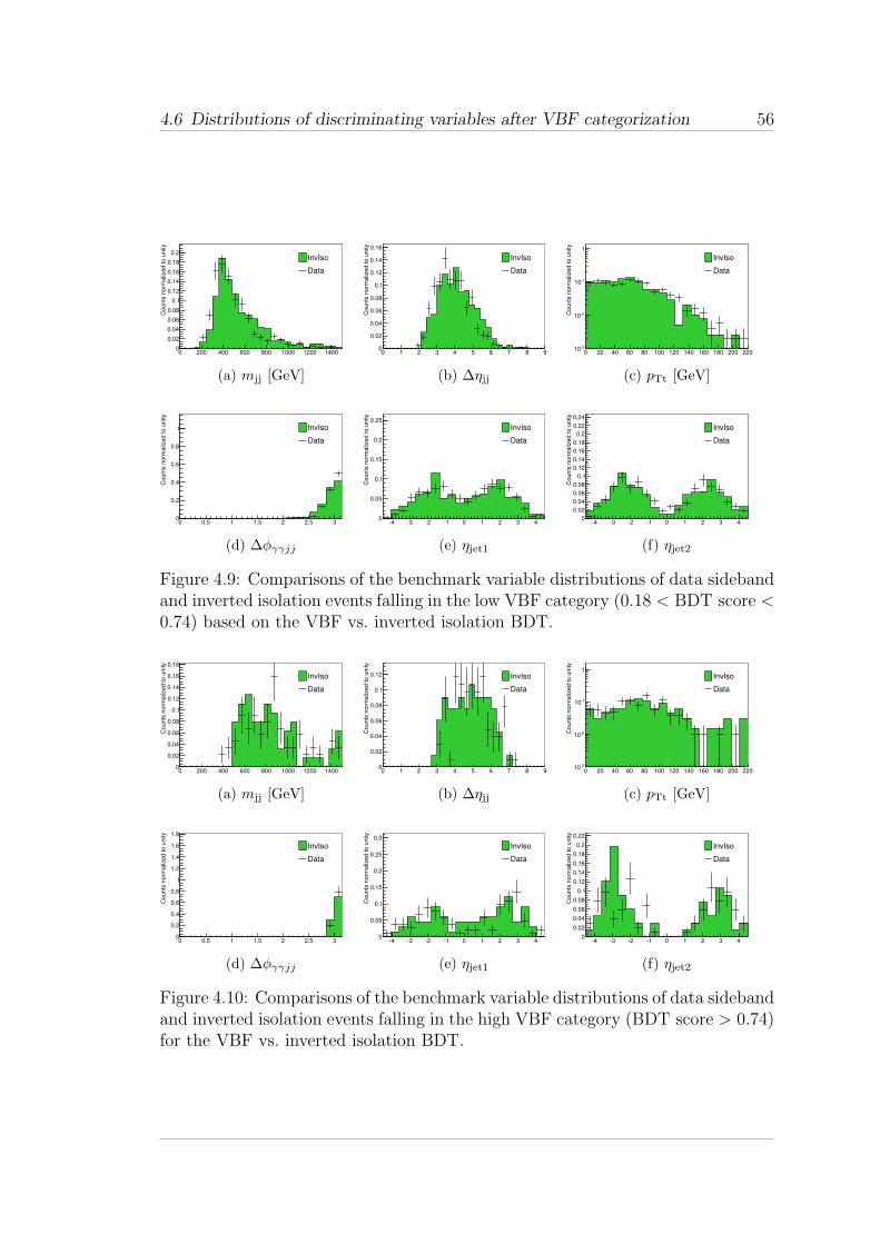
4.6 Distributions of discriminating variables after VBF categorization 56
0 200 400 600 800 1000 1200 1400
Counts
norm
aliz
ed to u
nity
0
0.02
0.04
0.06
0.08
0.1
0.12
0.14
0.16
0.18
0.2InvIso
Data
(a) mjj [GeV]
0 1 2 3 4 5 6 7 8 9
Counts
norm
aliz
ed to u
nity
0
0.02
0.04
0.06
0.08
0.1
0.12
0.14
0.16
InvIso
Data
(b) ∆ηjj
0 20 40 60 80 100 120 140 160 180 200 220
Counts
norm
aliz
ed to u
nity
-310
-210
-110
1
InvIso
Data
(c) pTt [GeV]
0 0.5 1 1.5 2 2.5 3
Counts
norm
aliz
ed to u
nity
0
0.2
0.4
0.6
0.8
1 InvIso
Data
(d) ∆φγγjj
-4 -3 -2 -1 0 1 2 3 4
Counts
norm
aliz
ed to u
nity
0
0.05
0.1
0.15
0.2
0.25
InvIso
Data
(e) ηjet1
-4 -3 -2 -1 0 1 2 3 4
Counts
norm
aliz
ed to u
nity
0
0.02
0.04
0.06
0.08
0.1
0.12
0.14
0.16
0.18
0.2
0.22
0.24
InvIso
Data
(f) ηjet2
Figure 4.9: Comparisons of the benchmark variable distributions of data sidebandand inverted isolation events falling in the low VBF category (0.18 < BDT score <0.74) based on the VBF vs. inverted isolation BDT.
0 200 400 600 800 1000 1200 1400
Counts
norm
aliz
ed to u
nity
0
0.02
0.04
0.06
0.08
0.1
0.12
0.14
0.16
0.18
InvIso
Data
(a) mjj [GeV]
0 1 2 3 4 5 6 7 8 9
Counts
norm
aliz
ed to u
nity
0
0.02
0.04
0.06
0.08
0.1
0.12 InvIso
Data
(b) ∆ηjj
0 20 40 60 80 100 120 140 160 180 200 220
Counts
norm
aliz
ed to u
nity
-310
-210
-110
1InvIso
Data
(c) pTt [GeV]
0 0.5 1 1.5 2 2.5 3
Counts
norm
aliz
ed to u
nity
0
0.2
0.4
0.6
0.8
1
1.2
1.4
1.6
1.8
InvIso
Data
(d) ∆φγγjj
-4 -3 -2 -1 0 1 2 3 4
Counts
norm
aliz
ed to u
nity
0
0.05
0.1
0.15
0.2
0.25
0.3
InvIso
Data
(e) ηjet1
-4 -3 -2 -1 0 1 2 3 4
Counts
norm
aliz
ed to u
nity
0
0.02
0.04
0.06
0.08
0.1
0.12
0.14
0.16
0.18
0.2
0.22
InvIso
Data
(f) ηjet2
Figure 4.10: Comparisons of the benchmark variable distributions of data sidebandand inverted isolation events falling in the high VBF category (BDT score > 0.74)for the VBF vs. inverted isolation BDT.
4.7 Checking for BDT sculpting in mγγ 57
4.7 Checking for BDT sculpting in mγγ
One major concern in the usage of a BDT-based analysis is the sculpting of kine-
matic distributions resultant from a hard cut on the BDT score. Here, the term
connotes a distortion of the shape of a given variable to the point where the initial
trend (i.e. prior to any BDT score cut) has been changed non-trivially, or a bias is
introduced to its expected value. The presence of this effect would be particularly
worrisome if occurring in the diphoton invariant mass distribution mγγ, as the
final analysis – in which discovery probability and signal strength are evaluated
for the VBF H → γγ process – is built around the expectation of a Gaussian-
like γγ signal ‘bump’ on top of a monotonically decreasing background. Therefore,
the presence of sculpting-like effects such as new peaks or non-monotony in the
mγγ sidebands (outside of statistical error) would cause significant difficulty in
merging the results of the VBF analysis with those of the other ATLAS H → γγ
groups.
For these reasons, it was necessary to check that no sculpting-like effects were
induced in the mγγ sidebands after successively tighter cuts on the BDT score.
A procedure to perform this check was developed and performed as follows. The
mγγ sidebands were divided up into four subsets, with each subset defined by a
BDT score range X1 < BDT score < X2, such that the range [X1, X2] contained
25% of the diphoton + dijet VBF signal Monte Carlo events – otherwise known as
‘quartiles’ of events. An exponential fit was then performed on each sideband data
subset, with the resultant distributions checked for sculpting-like effects, such as
new peaks in the mγγ distribution, or a monotonically increasing (or flat) fit. This
same procedure was then repeated using sideband data quartiles in lieu of VBF
Monte Carlo event quartiles.
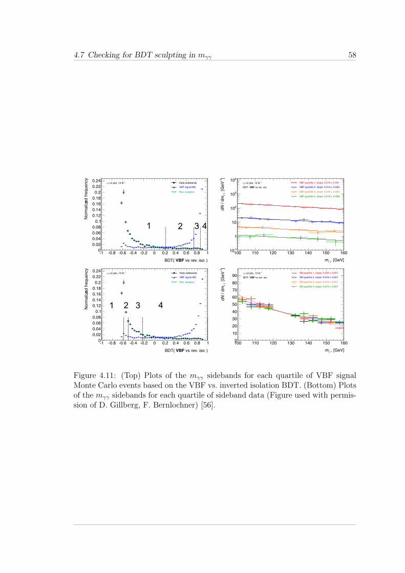
4.7 Checking for BDT sculpting in mγγ 58
)so.
)rev. iso. vs VBFBDT(
-1 -0.8 -0.6 -0.4 -0.2 0 0.2 0.4 0.6 0.8 1
Norm
aliz
ed f
requency
0
0.02
0.04
0.06
0.08
0.1
0.12
0.14
0.16
0.18
0.2
0.22
0.24 -1+2 jets, 13 fb!! Data sidebands
VBF signal MC
Rev. isolation
[GeV]!!m
100 110 120 130 140 150 160
]-1
[G
eV
!!
m /
dN
d
-110
1
10
210
310
410 0.001±VBF-quartile 1, slope: 0.016
0.002±VBF-quartile 2, slope: 0.014
0.004±VBF-quartile 3, slope: 0.016
0.008±VBF-quartile 4, slope: 0.015
-1+2 jets, 13 fb!!
rev. iso. vs VBFBDT:
1 2 3 4
)rev. iso. vs VBFBDT(
-1 -0.8 -0.6 -0.4 -0.2 0 0.2 0.4 0.6 0.8 1
Norm
aliz
ed f
requency
0
0.02
0.04
0.06
0.08
0.1
0.12
0.14
0.16
0.18
0.2
0.22
0.24 -1+2 jets, 13 fb!! Data sidebands
VBF signal MC
Rev. isolation
[GeV]!!m
100 110 120 130 140 150 160
]-1
[G
eV
!!
m /
dN
d
0
10
20
30
40
50
60
70
80
90 0.001±SB-quartile 1, slope: 0.020
0.001±SB-quartile 2, slope: 0.016
0.001±SB-quartile 3, slope: 0.014
0.001±SB-quartile 4, slope: 0.013
-1+2 jets, 13 fb!!
rev. iso. vs VBFBDT:
1 32 4
Figure 4.11: (Top) Plots of the mγγ sidebands for each quartile of VBF signalMonte Carlo events based on the VBF vs. inverted isolation BDT. (Bottom) Plotsof the mγγ sidebands for each quartile of sideband data (Figure used with permis-sion of D. Gillberg, F. Bernlochner) [56].
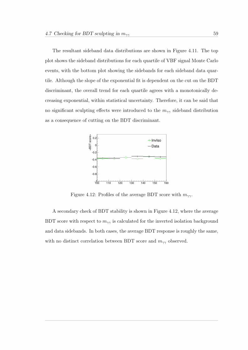
4.7 Checking for BDT sculpting in mγγ 59
The resultant sideband data distributions are shown in Figure 4.11. The top
plot shows the sideband distributions for each quartile of VBF signal Monte Carlo
events, with the bottom plot showing the sidebands for each sideband data quar-
tile. Although the slope of the exponential fit is dependent on the cut on the BDT
discriminant, the overall trend for each quartile agrees with a monotonically de-
creasing exponential, within statistical uncertainty. Therefore, it can be said that
no significant sculpting effects were introduced to the mγγ sideband distribution
as a consequence of cutting on the BDT discriminant.
100 110 120 130 140 150 160
<B
DT
score
>
-1
-0.8
-0.6
-0.4
-0.2
0
0.2InvIso
Data
Figure 4.12: Profiles of the average BDT score with mγγ.
A secondary check of BDT stability is shown in Figure 4.12, where the average
BDT score with respect to mγγ is calculated for the inverted isolation background
and data sidebands. In both cases, the average BDT response is roughly the same,
with no distinct correlation between BDT score and mγγ observed.
Chapter 5
Refining the VBF multivariate
analysis
Once the “rough” BDT-based analysis was established using inverted isolation
background, the next step was to refine the methodology to improve the efficacy
and efficiency of signal/background discrimination. To this end, many of the same
approaches detailed in Chapter 4 were enhanced with new choices of background
samples and variables, with the goal of improving the final VBF significance and
selection purity.
5.1 Improving the background model
A second option in deriving a background model, outside of using pure samples,
is to mix two (or more) of the samples described in Table 4.1, with each element
representing a unique component of the background. For example, one could use
Sherpa Monte Carlo events to represent the irreducible γγ background contribu-
tion, with another component handling the γj + jγ + jj elements. The primary
motivation for using such a mixture is the large sample statistics, which makes the
60
5.2 Improving benchmark variable selection 61
BDT less beholden to fluctuations in variable correlations and shape information
that may occur with small training samples. Furthermore, the more accurately
one is able to model the background, the more efficient and effective the BDT
discrimination becomes.
It was decided that any mixture of background components should be weighted
according to the approximate H → γγ background composition measured us-
ing the 2 × 1D fit method [58], which estimated a diphoton background com-
position of 79.5% γγ events, and 20.5% γj + jγ + jj events. Therefore, a new
background model was tested according to these guidelines, which mixed 79.5%
Sherpa γγ Monte Carlo events with 20.5% inverted isolation data, reweighted to
the statistics of the data sidebands. That is, the Sherpa component was weighted
to have 0.795×NSidebands effective events, while the inverted isolation component
was weighted to have 0.205×NSidebands effective events.
Figure 5.1 shows a comparison of the resultant kinematic distributions of the
Sherpa + inverted isolation mixture, as well as a pure inverted isolation sample,
with the data sidebands. While both background samples model the data side-
bands fairly well in terms of the dijet variables, these plots demonstrate that the
mixed sample improves greatly the agreement with sideband data for the diphoton
and dijet + diphoton variables. It was decided, then, to train another BDT using
this Sherpa + inverted isolation mixture to test its modelling capabilities.
5.2 Improving benchmark variable selection
It was initially decided that the original six benchmark variables should be in-
cluded in the refined BDT, having demonstrated their discriminating power in
Section 4.4.2. However, in an effort to garner the best performance out of the
BDT, additional variables and post-dijet selection cuts were also considered.
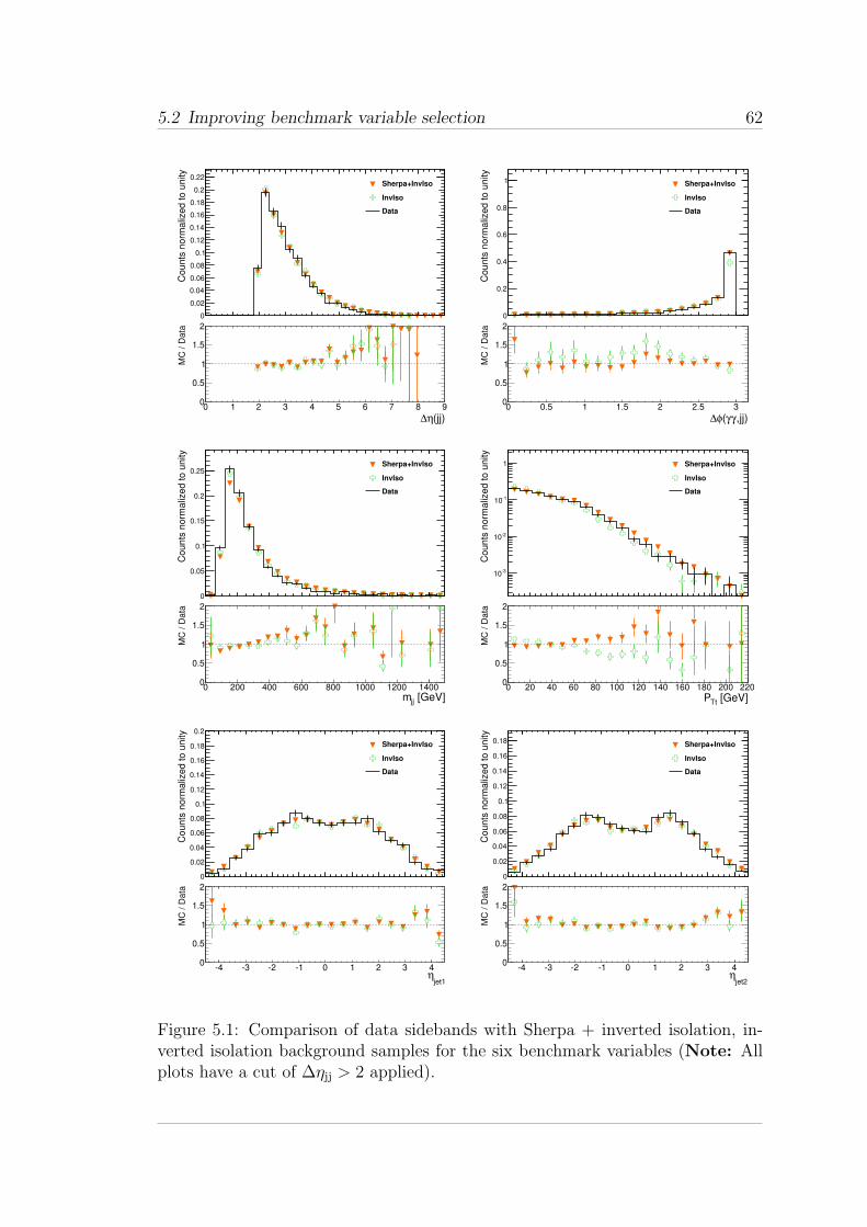
5.2 Improving benchmark variable selection 62
Co
un
ts n
orm
aliz
ed
to
un
ity
0
0.02
0.04
0.06
0.08
0.1
0.12
0.14
0.16
0.18
0.2
0.22Sherpa+InvIso
InvIso
Data
(jj)η∆0 1 2 3 4 5 6 7 8 9
MC
/ D
ata
0
0.5
1
1.5
2
Co
un
ts n
orm
aliz
ed
to
un
ity
0
0.2
0.4
0.6
0.8
1 Sherpa+InvIso
InvIso
Data
,jj)γγ(φ∆0 0.5 1 1.5 2 2.5 3
MC
/ D
ata
0
0.5
1
1.5
2
Co
un
ts n
orm
aliz
ed
to
un
ity
0
0.05
0.1
0.15
0.2
0.25Sherpa+InvIso
InvIso
Data
[GeV]jjm0 200 400 600 800 1000 1200 1400
MC
/ D
ata
0
0.5
1
1.5
2
Co
un
ts n
orm
aliz
ed
to
un
ity
-310
-210
-110
1 Sherpa+InvIso
InvIso
Data
[GeV]TtP0 20 40 60 80 100 120 140 160 180 200 220
MC
/ D
ata
0
0.5
1
1.5
2
Co
un
ts n
orm
aliz
ed
to
un
ity
0
0.02
0.04
0.06
0.08
0.1
0.12
0.14
0.16
0.18
0.2
Sherpa+InvIso
InvIso
Data
jet1η
-4 -3 -2 -1 0 1 2 3 4
MC
/ D
ata
0
0.5
1
1.5
2
Co
un
ts n
orm
aliz
ed
to
un
ity
0
0.02
0.04
0.06
0.08
0.1
0.12
0.14
0.16
0.18 Sherpa+InvIso
InvIso
Data
jet2η
-4 -3 -2 -1 0 1 2 3 4
MC
/ D
ata
0
0.5
1
1.5
2
Figure 5.1: Comparison of data sidebands with Sherpa + inverted isolation, in-verted isolation background samples for the six benchmark variables (Note: Allplots have a cut of ∆ηjj > 2 applied).
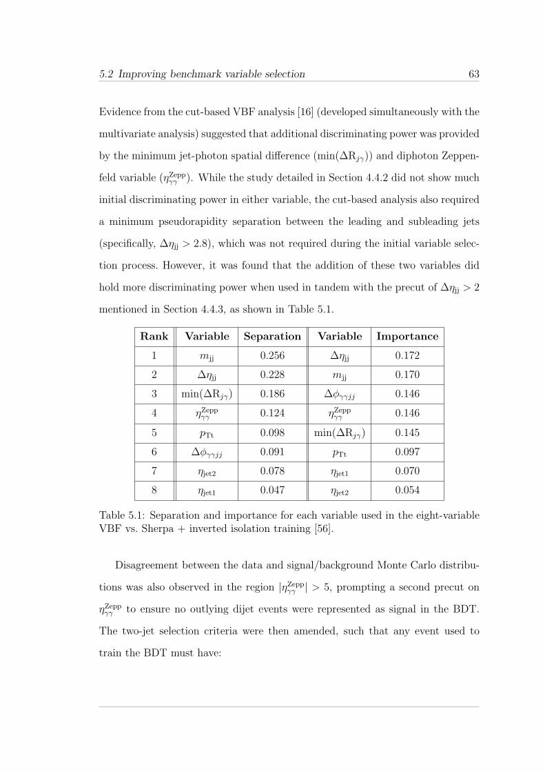
5.2 Improving benchmark variable selection 63
Evidence from the cut-based VBF analysis [16] (developed simultaneously with the
multivariate analysis) suggested that additional discriminating power was provided
by the minimum jet-photon spatial difference (min(∆Rjγ)) and diphoton Zeppen-
feld variable (ηZeppγγ ). While the study detailed in Section 4.4.2 did not show much
initial discriminating power in either variable, the cut-based analysis also required
a minimum pseudorapidity separation between the leading and subleading jets
(specifically, ∆ηjj > 2.8), which was not required during the initial variable selec-
tion process. However, it was found that the addition of these two variables did
hold more discriminating power when used in tandem with the precut of ∆ηjj > 2
mentioned in Section 4.4.3, as shown in Table 5.1.
Rank Variable Separation Variable Importance
1 mjj 0.256 ∆ηjj 0.172
2 ∆ηjj 0.228 mjj 0.170
3 min(∆Rjγ) 0.186 ∆φγγjj 0.146
4 ηZeppγγ 0.124 ηZeppγγ 0.146
5 pTt 0.098 min(∆Rjγ) 0.145
6 ∆φγγjj 0.091 pTt 0.097
7 ηjet2 0.078 ηjet1 0.070
8 ηjet1 0.047 ηjet2 0.054
Table 5.1: Separation and importance for each variable used in the eight-variableVBF vs. Sherpa + inverted isolation training [56].
Disagreement between the data and signal/background Monte Carlo distribu-
tions was also observed in the region |ηZeppγγ | > 5, prompting a second precut on
ηZeppγγ to ensure no outlying dijet events were represented as signal in the BDT.
The two-jet selection criteria were then amended, such that any event used to
train the BDT must have:
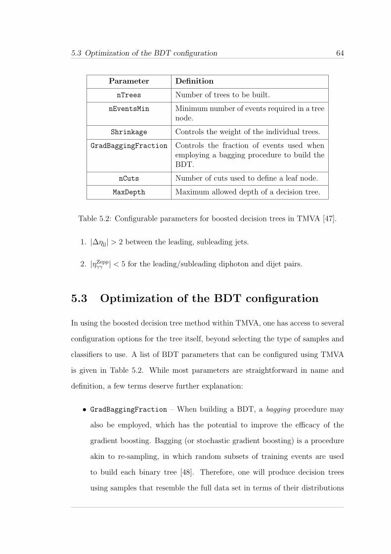
5.3 Optimization of the BDT configuration 64
Parameter Definition
nTrees Number of trees to be built.
nEventsMin Minimum number of events required in a treenode.
Shrinkage Controls the weight of the individual trees.
GradBaggingFraction Controls the fraction of events used whenemploying a bagging procedure to build theBDT.
nCuts Number of cuts used to define a leaf node.
MaxDepth Maximum allowed depth of a decision tree.
Table 5.2: Configurable parameters for boosted decision trees in TMVA [47].
1. |∆ηjj| > 2 between the leading, subleading jets.
2. |ηZeppγγ | < 5 for the leading/subleading diphoton and dijet pairs.
5.3 Optimization of the BDT configuration
In using the boosted decision tree method within TMVA, one has access to several
configuration options for the tree itself, beyond selecting the type of samples and
classifiers to use. A list of BDT parameters that can be configured using TMVA
is given in Table 5.2. While most parameters are straightforward in name and
definition, a few terms deserve further explanation:
• GradBaggingFraction – When building a BDT, a bagging procedure may
also be employed, which has the potential to improve the efficacy of the
gradient boosting. Bagging (or stochastic gradient boosting) is a procedure
akin to re-sampling, in which random subsets of training events are used
to build each binary tree [48]. Therefore, one will produce decision trees
using samples that resemble the full data set in terms of their distributions
5.3 Optimization of the BDT configuration 65
and variance, but are effectively unique. In theory, the usage of this pro-
cedure will lead to more statistical stability in the classifier, depending on
the fraction of events used in the bagging (a fraction between 0.5 and 0.8 is
recommended [47]).
• Shrinkage – The robustness of a BDT is controlled by the shrinkage, or
nominal weight, of the individual trees. This factor can be compared to the
learning rate of the BDT, and its size should be relative to the number of
trees being grown (nTrees), i.e. A smaller shrinkage (e.g. 0.1 - 0.3) requires
more trees to be grown [47].
• MaxDepth – This parameter controls the maximum number of decisions that
can be made by each tree. After MaxDepth number of decisions has been
reached by a given branch, a node is reached, with a signal/background
decision made.
Because there are several parameters with which the structure of the BDT can be
modified, it became necessary to ensure that the BDT-based analysis was actually
using the most optimal configuration possible. In theory, the best configuration
of the BDT would provide statistical stability, not detract from the established
discriminating power, and, if possible, improve signal/background identification
for the particular samples chosen.
Similar to the input variable optimization method described in Section 4.4.2,
a multivariable scan was performed for the BDT input parameters. A list of the
parameters tested, along with the values for the scan, is given in Table 5.3, which
amounts to a total of 2880 combinations of input parameters. For each configu-
ration, a BDT was trained using a VBF H → γγ signal Monte Carlo sample and
Sherpa + inverted isolation background, as described in Section 5.1, divided using
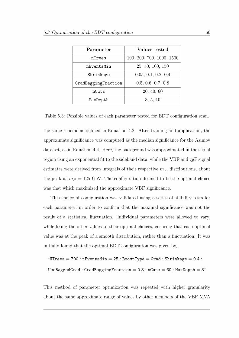
5.3 Optimization of the BDT configuration 66
Parameter Values tested
nTrees 100, 200, 700, 1000, 1500
nEventsMin 25, 50, 100, 150
Shrinkage 0.05, 0.1, 0.2, 0.4
GradBaggingFraction 0.5, 0.6, 0.7, 0.8
nCuts 20, 40, 60
MaxDepth 3, 5, 10
Table 5.3: Possible values of each parameter tested for BDT configuration scan.
the same scheme as defined in Equation 4.2. After training and application, the
approximate significance was computed as the median significance for the Asimov
data set, as in Equation 4.4. Here, the background was approximated in the signal
region using an exponential fit to the sideband data, while the VBF and ggF signal
estimates were derived from integrals of their respective mγγ distributions, about
the peak at mH = 125 GeV. The configuration deemed to be the optimal choice
was that which maximized the approximate VBF significance.
This choice of configuration was validated using a series of stability tests for
each parameter, in order to confirm that the maximal significance was not the
result of a statistical fluctuation. Individual parameters were allowed to vary,
while fixing the other values to their optimal choices, ensuring that each optimal
value was at the peak of a smooth distribution, rather than a fluctuation. It was
initially found that the optimal BDT configuration was given by,
“NTrees = 700 : nEventsMin = 25 : BoostType = Grad : Shrinkage = 0.4 :
UseBaggedGrad : GradBaggingFraction = 0.8 : nCuts = 60 : MaxDepth = 3”
This method of parameter optimization was repeated with higher granularity
about the same approximate range of values by other members of the VBF MVA
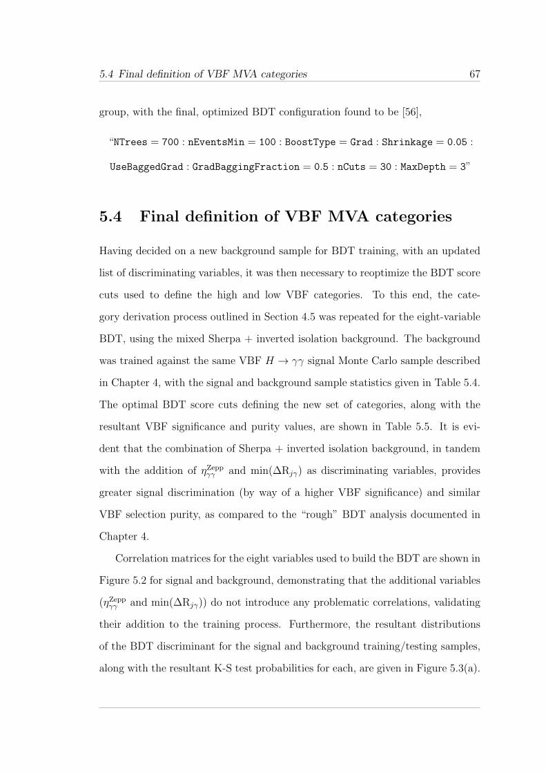
5.4 Final definition of VBF MVA categories 67
group, with the final, optimized BDT configuration found to be [56],
“NTrees = 700 : nEventsMin = 100 : BoostType = Grad : Shrinkage = 0.05 :
UseBaggedGrad : GradBaggingFraction = 0.5 : nCuts = 30 : MaxDepth = 3”
5.4 Final definition of VBF MVA categories
Having decided on a new background sample for BDT training, with an updated
list of discriminating variables, it was then necessary to reoptimize the BDT score
cuts used to define the high and low VBF categories. To this end, the cate-
gory derivation process outlined in Section 4.5 was repeated for the eight-variable
BDT, using the mixed Sherpa + inverted isolation background. The background
was trained against the same VBF H → γγ signal Monte Carlo sample described
in Chapter 4, with the signal and background sample statistics given in Table 5.4.
The optimal BDT score cuts defining the new set of categories, along with the
resultant VBF significance and purity values, are shown in Table 5.5. It is evi-
dent that the combination of Sherpa + inverted isolation background, in tandem
with the addition of ηZeppγγ and min(∆Rjγ) as discriminating variables, provides
greater signal discrimination (by way of a higher VBF significance) and similar
VBF selection purity, as compared to the “rough” BDT analysis documented in
Chapter 4.
Correlation matrices for the eight variables used to build the BDT are shown in
Figure 5.2 for signal and background, demonstrating that the additional variables
(ηZeppγγ and min(∆Rjγ)) do not introduce any problematic correlations, validating
their addition to the training process. Furthermore, the resultant distributions
of the BDT discriminant for the signal and background training/testing samples,
along with the resultant K-S test probabilities for each, are given in Figure 5.3(a).
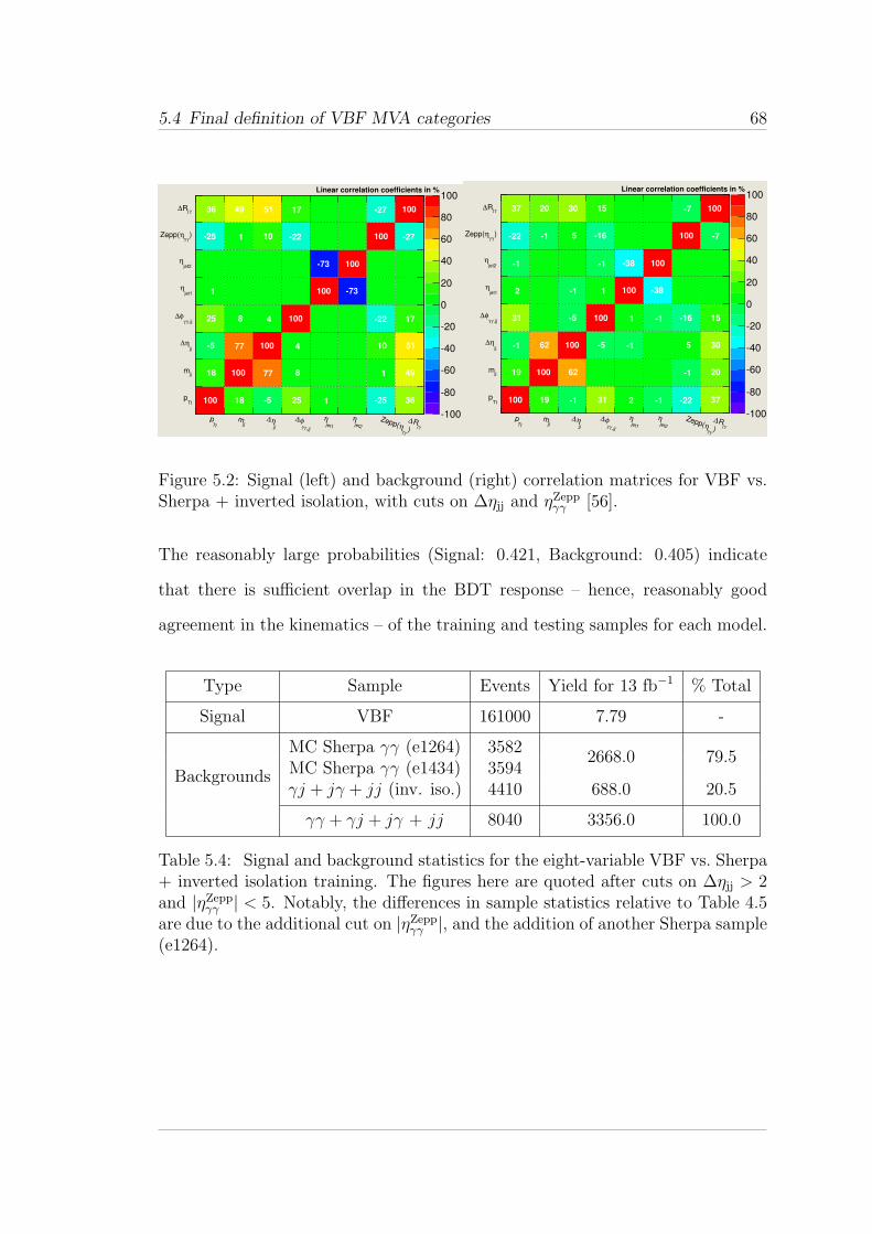
5.4 Final definition of VBF MVA categories 68
-100
-80
-60
-40
-20
0
20
40
60
80
100
Tt
pjj
mjj
η∆
,jjγγ
φ∆jet1
ηjet2
η
)γγ
ηZepp( γj
R∆
Ttp
jjm
jjη∆
,jjγγφ∆
jet1η
jet2η
)γγ
ηZepp(
γjR∆
100 18 -5 25 1 -25 36
18 100 77 8 1 49
-5 77 100 4 10 51
25 8 4 100 -22 17
1 100 -73
-73 100
-25 1 10 -22 100 -27
36 49 51 17 -27 100
Linear correlation coefficients in %
-100
-80
-60
-40
-20
0
20
40
60
80
100
Tt
pjj
mjj
η∆
,jjγγ
φ∆jet1
ηjet2
η
)γγ
ηZepp( γj
R∆
Ttp
jjm
jjη∆
,jjγγφ∆
jet1η
jet2η
)γγ
ηZepp(
γjR∆
100 19 -1 31 2 -1 -22 37
19 100 62 -1 20
-1 62 100 -5 -1 5 30
31 -5 100 1 -1 -16 15
2 -1 1 100 -38
-1 -1 -38 100
-22 -1 5 -16 100 -7
37 20 30 15 -7 100
Linear correlation coefficients in %
Figure 5.2: Signal (left) and background (right) correlation matrices for VBF vs.Sherpa + inverted isolation, with cuts on ∆ηjj and η
Zeppγγ [56].
The reasonably large probabilities (Signal: 0.421, Background: 0.405) indicate
that there is sufficient overlap in the BDT response – hence, reasonably good
agreement in the kinematics – of the training and testing samples for each model.
Type Sample Events Yield for 13 fb−1 % Total
Signal VBF 161000 7.79 -
Backgrounds
MC Sherpa γγ (e1264) 35822668.0 79.5
MC Sherpa γγ (e1434) 3594γj + jγ + jj (inv. iso.) 4410 688.0 20.5
γγ + γj + jγ + jj 8040 3356.0 100.0
Table 5.4: Signal and background statistics for the eight-variable VBF vs. Sherpa+ inverted isolation training. The figures here are quoted after cuts on ∆ηjj > 2and |ηZeppγγ | < 5. Notably, the differences in sample statistics relative to Table 4.5are due to the additional cut on |ηZeppγγ |, and the addition of another Sherpa sample(e1264).
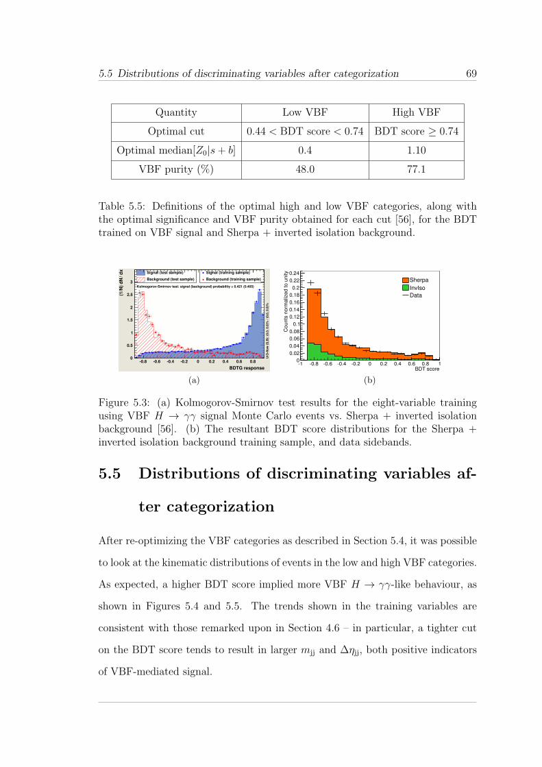
5.5 Distributions of discriminating variables after categorization 69
Quantity Low VBF High VBF
Optimal cut 0.44 < BDT score < 0.74 BDT score ≥ 0.74
Optimal median[Z0|s+ b] 0.4 1.10
VBF purity (%) 48.0 77.1
Table 5.5: Definitions of the optimal high and low VBF categories, along withthe optimal significance and VBF purity obtained for each cut [56], for the BDTtrained on VBF signal and Sherpa + inverted isolation background.
BDTG response
-0.8 -0.6 -0.4 -0.2 0 0.2 0.4 0.6 0.8
dx
/ (1
/N)
dN
0
0.5
1
1.5
2
2.5
3
Signal (test sample)
Background (test sample)
Signal (training sample)
Background (training sample)
Kolmogorov-Smirnov test: signal (background) probability = 0.421 (0.405)
U/O
-flo
w (
S,B
): (
0.0
, 0
.0)%
/ (
0.0
, 0
.0)%
(a)
BDT score-1 -0.8 -0.6 -0.4 -0.2 0 0.2 0.4 0.6 0.8 1
Co
un
ts n
orm
aliz
ed
to
un
ity
0
0.02
0.04
0.06
0.08
0.1
0.12
0.14
0.16
0.18
0.2
0.22
0.24
Sherpa
InvIso
Data
(b)
Figure 5.3: (a) Kolmogorov-Smirnov test results for the eight-variable trainingusing VBF H → γγ signal Monte Carlo events vs. Sherpa + inverted isolationbackground [56]. (b) The resultant BDT score distributions for the Sherpa +inverted isolation background training sample, and data sidebands.
5.5 Distributions of discriminating variables af-
ter categorization
After re-optimizing the VBF categories as described in Section 5.4, it was possible
to look at the kinematic distributions of events in the low and high VBF categories.
As expected, a higher BDT score implied more VBF H → γγ-like behaviour, as
shown in Figures 5.4 and 5.5. The trends shown in the training variables are
consistent with those remarked upon in Section 4.6 – in particular, a tighter cut
on the BDT score tends to result in larger mjj and ∆ηjj, both positive indicators
of VBF-mediated signal.
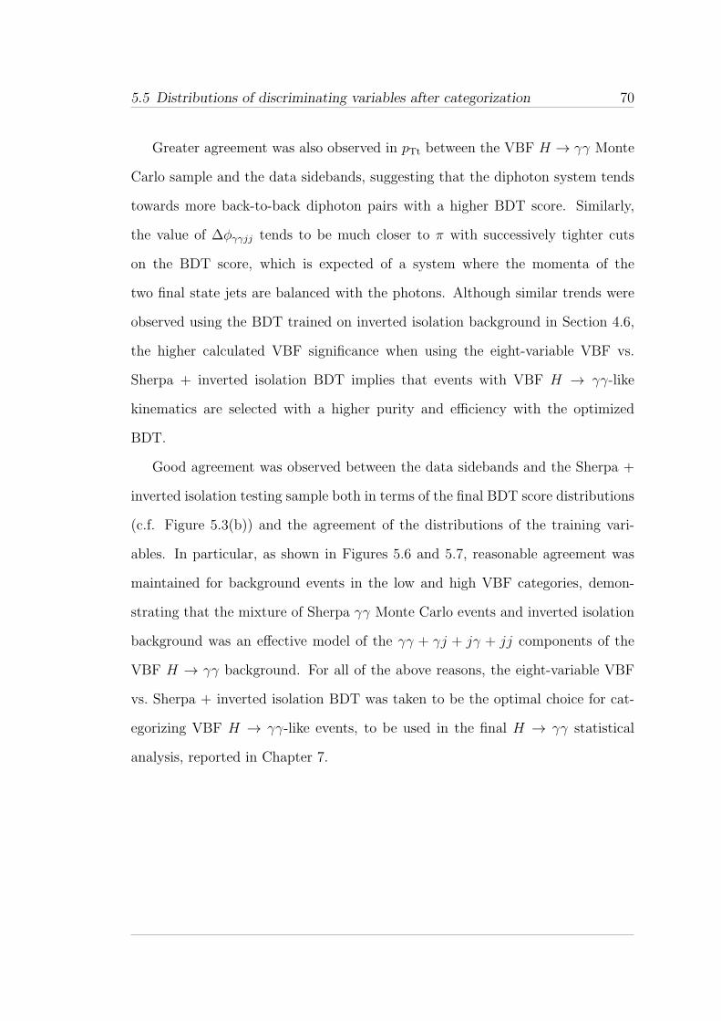
5.5 Distributions of discriminating variables after categorization 70
Greater agreement was also observed in pTt between the VBF H → γγ Monte
Carlo sample and the data sidebands, suggesting that the diphoton system tends
towards more back-to-back diphoton pairs with a higher BDT score. Similarly,
the value of ∆φγγjj tends to be much closer to π with successively tighter cuts
on the BDT score, which is expected of a system where the momenta of the
two final state jets are balanced with the photons. Although similar trends were
observed using the BDT trained on inverted isolation background in Section 4.6,
the higher calculated VBF significance when using the eight-variable VBF vs.
Sherpa + inverted isolation BDT implies that events with VBF H → γγ-like
kinematics are selected with a higher purity and efficiency with the optimized
BDT.
Good agreement was observed between the data sidebands and the Sherpa +
inverted isolation testing sample both in terms of the final BDT score distributions
(c.f. Figure 5.3(b)) and the agreement of the distributions of the training vari-
ables. In particular, as shown in Figures 5.6 and 5.7, reasonable agreement was
maintained for background events in the low and high VBF categories, demon-
strating that the mixture of Sherpa γγ Monte Carlo events and inverted isolation
background was an effective model of the γγ + γj + jγ + jj components of the
VBF H → γγ background. For all of the above reasons, the eight-variable VBF
vs. Sherpa + inverted isolation BDT was taken to be the optimal choice for cat-
egorizing VBF H → γγ-like events, to be used in the final H → γγ statistical
analysis, reported in Chapter 7.
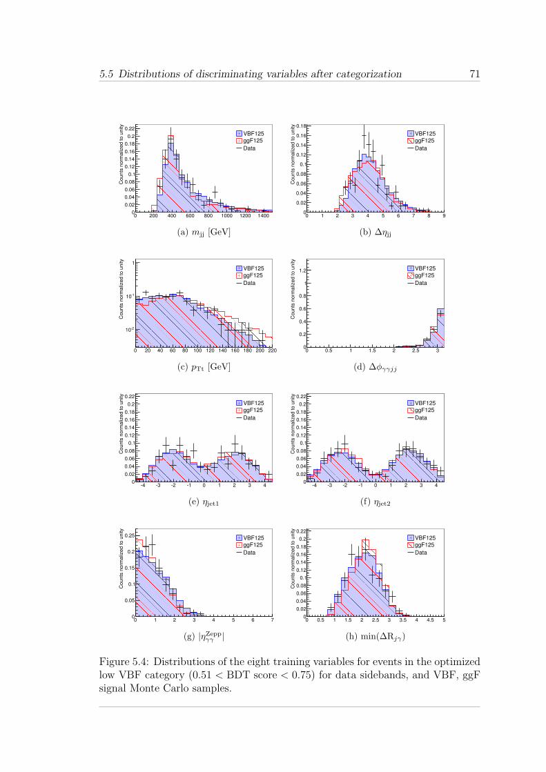
5.5 Distributions of discriminating variables after categorization 71
0 200 400 600 800 1000 1200 1400
Counts
norm
aliz
ed to u
nity
0
0.02
0.04
0.06
0.08
0.1
0.12
0.14
0.16
0.18
0.2
0.22VBF125
ggF125
Data
(a) mjj [GeV]
0 1 2 3 4 5 6 7 8 9
Counts
norm
aliz
ed to u
nity
0
0.02
0.04
0.06
0.08
0.1
0.12
0.14
0.16
0.18
VBF125
ggF125
Data
(b) ∆ηjj
0 20 40 60 80 100 120 140 160 180 200 220
Counts
norm
aliz
ed to u
nity
-210
-110
1VBF125
ggF125
Data
(c) pTt [GeV]
0 0.5 1 1.5 2 2.5 3
Counts
norm
aliz
ed to u
nity
0
0.2
0.4
0.6
0.8
1
1.2 VBF125
ggF125
Data
(d) ∆φγγjj
-4 -3 -2 -1 0 1 2 3 4
Counts
norm
aliz
ed to u
nity
0
0.02
0.04
0.06
0.08
0.1
0.12
0.14
0.16
0.18
0.2
0.22
VBF125
ggF125
Data
(e) ηjet1
-4 -3 -2 -1 0 1 2 3 4
Counts
norm
aliz
ed to u
nity
0
0.02
0.04
0.06
0.08
0.1
0.12
0.14
0.16
0.18
0.2
0.22
VBF125
ggF125
Data
(f) ηjet2
0 1 2 3 4 5 6 7
Counts
norm
aliz
ed to u
nity
0
0.05
0.1
0.15
0.2
0.25 VBF125
ggF125
Data
(g) |ηZeppγγ |
0 0.5 1 1.5 2 2.5 3 3.5 4 4.5 5
Counts
norm
aliz
ed to u
nity
0
0.02
0.04
0.06
0.08
0.1
0.12
0.14
0.16
0.18
0.2
0.22
VBF125
ggF125
Data
(h) min(∆Rjγ)
Figure 5.4: Distributions of the eight training variables for events in the optimizedlow VBF category (0.51 < BDT score < 0.75) for data sidebands, and VBF, ggFsignal Monte Carlo samples.
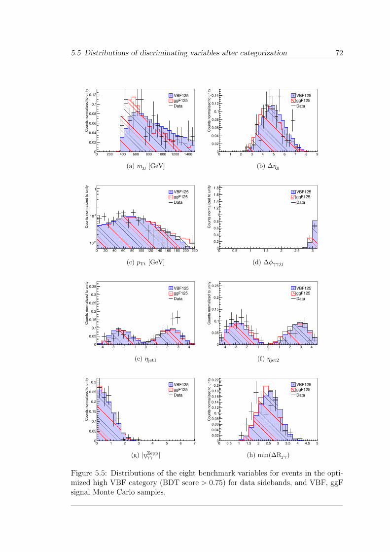
5.5 Distributions of discriminating variables after categorization 72
0 200 400 600 800 1000 1200 1400
Counts
norm
aliz
ed to u
nity
0
0.02
0.04
0.06
0.08
0.1
0.12 VBF125
ggF125
Data
(a) mjj [GeV]
0 1 2 3 4 5 6 7 8 9
Counts
norm
aliz
ed to u
nity
0
0.02
0.04
0.06
0.08
0.1
0.12
0.14 VBF125
ggF125
Data
(b) ∆ηjj
0 20 40 60 80 100 120 140 160 180 200 220
Counts
norm
aliz
ed to u
nity
-210
-110
1VBF125
ggF125
Data
(c) pTt [GeV]
0 0.5 1 1.5 2 2.5 3
Counts
norm
aliz
ed to u
nity
0
0.2
0.4
0.6
0.8
1
1.2
1.4
1.6
1.8VBF125
ggF125
Data
(d) ∆φγγjj
-4 -3 -2 -1 0 1 2 3 4
Counts
norm
aliz
ed to u
nity
0
0.05
0.1
0.15
0.2
0.25
0.3
0.35 VBF125
ggF125
Data
(e) ηjet1
-4 -3 -2 -1 0 1 2 3 4
Counts
norm
aliz
ed to u
nity
0
0.05
0.1
0.15
0.2
0.25VBF125
ggF125
Data
(f) ηjet2
0 1 2 3 4 5 6 7
Counts
norm
aliz
ed to u
nity
0
0.05
0.1
0.15
0.2
0.25
0.3VBF125
ggF125
Data
(g) |ηZeppγγ |
0 0.5 1 1.5 2 2.5 3 3.5 4 4.5 5
Counts
norm
aliz
ed to u
nity
0
0.02
0.04
0.06
0.08
0.1
0.12
0.14
0.16
0.18
0.2
0.22
VBF125
ggF125
Data
(h) min(∆Rjγ)
Figure 5.5: Distributions of the eight benchmark variables for events in the opti-mized high VBF category (BDT score > 0.75) for data sidebands, and VBF, ggFsignal Monte Carlo samples.
5.5 Distributions of discriminating variables after categorization 73
0 200 400 600 800 1000 1200 1400
Counts
norm
aliz
ed to u
nity
0
0.02
0.04
0.06
0.08
0.1
0.12
0.14
0.16
0.18
0.2
0.22 Sherpa
InvIso
Data
(a) mjj [GeV]
0 1 2 3 4 5 6 7 8 9
Counts
norm
aliz
ed to u
nity
0
0.02
0.04
0.06
0.08
0.1
0.12
0.14
0.16
0.18
Sherpa
InvIso
Data
(b) ∆ηjj
0 20 40 60 80 100 120 140 160 180 200 220
Counts
norm
aliz
ed to u
nity
-310
-210
-110
1Sherpa
InvIso
Data
(c) pTt [GeV]
0 0.5 1 1.5 2 2.5 3
Counts
norm
aliz
ed to u
nity
0
0.2
0.4
0.6
0.8
1
1.2
Sherpa
InvIso
Data
(d) ∆φγγjj
-4 -3 -2 -1 0 1 2 3 4
Counts
norm
aliz
ed to u
nity
0
0.02
0.04
0.06
0.08
0.1
0.12
0.14
0.16
0.18
0.2
0.22
Sherpa
InvIso
Data
(e) ηjet1
-4 -3 -2 -1 0 1 2 3 4
Counts
norm
aliz
ed to u
nity
0
0.02
0.04
0.06
0.08
0.1
0.12
0.14
0.16
0.18
0.2
0.22
Sherpa
InvIso
Data
(f) ηjet2
0 1 2 3 4 5 6 7
Counts
norm
aliz
ed to u
nity
0
0.05
0.1
0.15
0.2
0.25
Sherpa
InvIso
Data
(g) |ηZeppγγ |
0 0.5 1 1.5 2 2.5 3 3.5 4 4.5 5
Counts
norm
aliz
ed to u
nity
0
0.02
0.04
0.06
0.08
0.1
0.12
0.14
0.16
0.18 Sherpa
InvIso
Data
(h) min(∆Rjγ)
Figure 5.6: Comparisons of the benchmark variable distributions of data side-band and Sherpa + inverted isolation events in the low VBF category (0.51 <BDT score < 0.74) for the VBF vs. Sherpa + inverted isolation BDT.
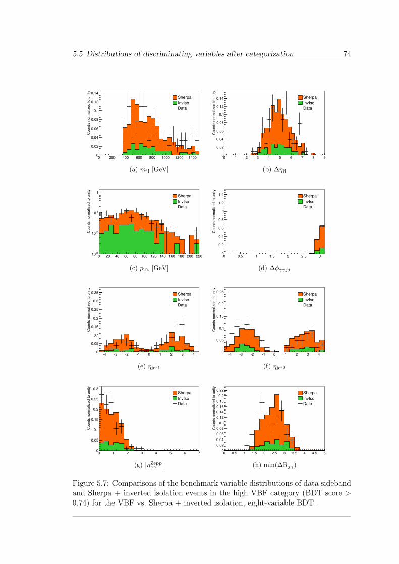
5.5 Distributions of discriminating variables after categorization 74
0 200 400 600 800 1000 1200 1400
Counts
norm
aliz
ed to u
nity
0
0.02
0.04
0.06
0.08
0.1
0.12
0.14Sherpa
InvIso
Data
(a) mjj [GeV]
0 1 2 3 4 5 6 7 8 9
Counts
norm
aliz
ed to u
nity
0
0.02
0.04
0.06
0.08
0.1
0.12
0.14 Sherpa
InvIso
Data
(b) ∆ηjj
0 20 40 60 80 100 120 140 160 180 200 220
Counts
norm
aliz
ed to u
nity
-310
-210
-110
1Sherpa
InvIso
Data
(c) pTt [GeV]
0 0.5 1 1.5 2 2.5 3
Counts
norm
aliz
ed to u
nity
0
0.2
0.4
0.6
0.8
1
1.2
1.4 Sherpa
InvIso
Data
(d) ∆φγγjj
-4 -3 -2 -1 0 1 2 3 4
Counts
norm
aliz
ed to u
nity
0
0.05
0.1
0.15
0.2
0.25
0.3
0.35 Sherpa
InvIso
Data
(e) ηjet1
-4 -3 -2 -1 0 1 2 3 4
Counts
norm
aliz
ed to u
nity
0
0.05
0.1
0.15
0.2
0.25Sherpa
InvIso
Data
(f) ηjet2
0 1 2 3 4 5 6 7
Counts
norm
aliz
ed to u
nity
0
0.05
0.1
0.15
0.2
0.25
0.3Sherpa
InvIso
Data
(g) |ηZeppγγ |
0 0.5 1 1.5 2 2.5 3 3.5 4 4.5 5
Counts
norm
aliz
ed to u
nity
0
0.02
0.04
0.06
0.08
0.1
0.12
0.14
0.16
0.18
0.2
0.22Sherpa
InvIso
Data
(h) min(∆Rjγ)
Figure 5.7: Comparisons of the benchmark variable distributions of data sidebandand Sherpa + inverted isolation events in the high VBF category (BDT score >0.74) for the VBF vs. Sherpa + inverted isolation, eight-variable BDT.
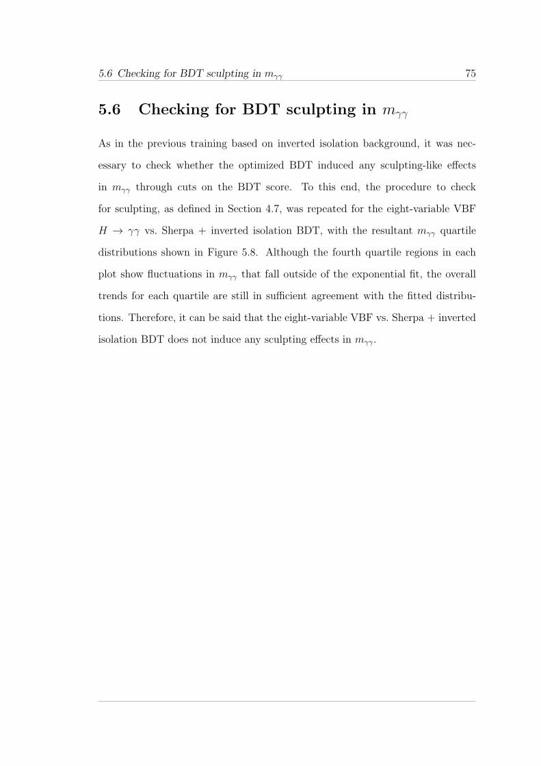
5.6 Checking for BDT sculpting in mγγ 75
5.6 Checking for BDT sculpting in mγγ
As in the previous training based on inverted isolation background, it was nec-
essary to check whether the optimized BDT induced any sculpting-like effects
in mγγ through cuts on the BDT score. To this end, the procedure to check
for sculpting, as defined in Section 4.7, was repeated for the eight-variable VBF
H → γγ vs. Sherpa + inverted isolation BDT, with the resultant mγγ quartile
distributions shown in Figure 5.8. Although the fourth quartile regions in each
plot show fluctuations in mγγ that fall outside of the exponential fit, the overall
trends for each quartile are still in sufficient agreement with the fitted distribu-
tions. Therefore, it can be said that the eight-variable VBF vs. Sherpa + inverted
isolation BDT does not induce any sculpting effects in mγγ.
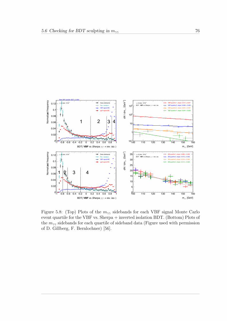
5.6 Checking for BDT sculpting in mγγ 76
) + rev. iso.!!Sherpa vs VBFBDT(
-1 -0.8 -0.6 -0.4 -0.2 0 0.2 0.4 0.6 0.8 1
Norm
aliz
ed f
requency
0
0.02
0.04
0.06
0.08
0.1
0.12-1+2 jets, 13 fb!! Data sidebands
VBF signal MC
Rev. isolation
ggH signal MC
Best VBF-quartile: BDT > 0.854
[GeV]!!m
100 110 120 130 140 150 160
]-1
[G
eV
!!
m /
dN
d
-110
1
10
210
310
0.001±VBF-quartile 1, slope: 0.017
0.003±VBF-quartile 2, slope: 0.009
0.007±VBF-quartile 3, slope: 0.021
0.035±VBF-quartile 4, slope: 0.044
-1+2 jets, 13 fb!!
+ rev. iso.!!Sherpa vs VBFBDT:
ncy 0.24
]-1
V
410
1 2 3 4
) + rev. iso.!!Sherpa vs VBFBDT(
-1 -0.8 -0.6 -0.4 -0.2 0 0.2 0.4 0.6 0.8 1
Norm
aliz
ed f
requency
0
0.02
0.04
0.06
0.08
0.1
0.12-1+2 jets, 13 fb!! Data sidebands
VBF signal MC
Rev. isolation
ggH signal MC
[GeV]!!m
100 110 120 130 140 150 160
]-1
[G
eV
!!
m /
dN
d
0
5
10
15
20
25
30
35 0.002±SB-quartile 1, slope: 0.023
0.002±SB-quartile 2, slope: 0.013
0.002±SB-quartile 3, slope: 0.016
0.002±SB-quartile 4, slope: 0.014
-1+2 jets, 13 fb!!
+ rev. iso.!!Sherpa vs VBFBDT:
1 2 3 4
Figure 5.8: (Top) Plots of the mγγ sidebands for each VBF signal Monte Carloevent quartile for the VBF vs. Sherpa + inverted isolation BDT. (Bottom) Plots ofthe mγγ sidebands for each quartile of sideband data (Figure used with permissionof D. Gillberg, F. Bernlochner) [56].
5.6 Checking for BDT sculpting in mγγ 77
[GeV]γγm100 110 120 130 140 150 160
<B
DT
score
>
-1
-0.8
-0.6
-0.4
-0.2
0
0.2 Sherpa
InvIso
Data
Figure 5.9: Profiles of the average BDT score with mγγ.
A secondary check of BDT stability is shown in Figure 5.9, where the average
BDT score with respect to mγγ is calculated for each component of the Sherpa +
inverted isolation background, as well as the data sidebands. In each sample, the
average BDT response is roughly the same, with no distinct correlation between
BDT score and mγγ observed.
Chapter 6
Systematic uncertainties
The careful evaluation of systematic uncertainties is crucial for any physics anal-
ysis, as any measurement or scientific claim – especially as it relates to the agree-
ment with (or deviation from) a physical model – must be made relative to the
bounds of systematic and statistical error. In ATLAS, systematic uncertainties are
defined relative to Standard Model yield predictions, and are propagated through
to the final statistical analysis as nuisance parameters (see Chapter 7). The sys-
tematic uncertainties in the VBF H → γγ analysis are both theoretical, derived
from variable modelling and perturbative uncertainties, and experimental, emerg-
ing from detector effects, object reconstruction, and energy calibration.
6.1 Theoretical uncertainties
6.1.1 Higher-order perturbative uncertainty for gg → H +
2 jets
As alluded to in Section 2.5.1, the usage of dijet + diphoton variables such as
∆φγγjj must be carefully considered with regard to the gg → H + 2 jet cross
section. In applying cuts to isolate VBF-like signal using such a variable, one
78
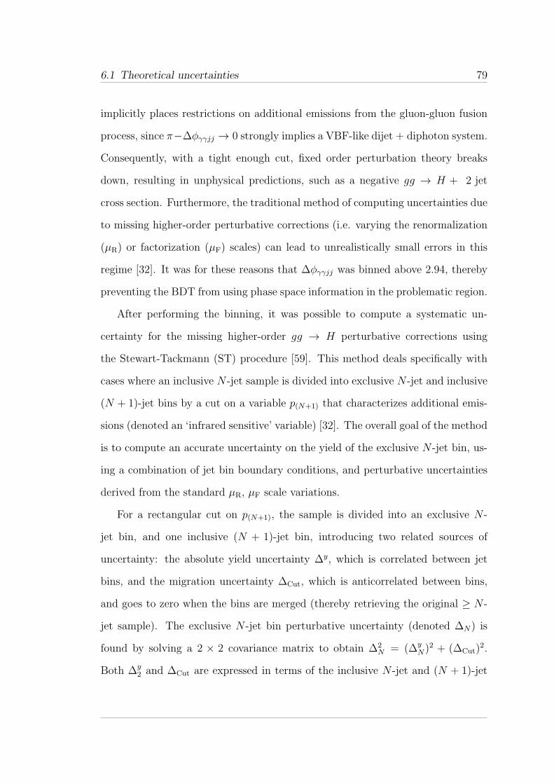
6.1 Theoretical uncertainties 79
implicitly places restrictions on additional emissions from the gluon-gluon fusion
process, since π−∆φγγjj → 0 strongly implies a VBF-like dijet + diphoton system.
Consequently, with a tight enough cut, fixed order perturbation theory breaks
down, resulting in unphysical predictions, such as a negative gg → H + 2 jet
cross section. Furthermore, the traditional method of computing uncertainties due
to missing higher-order perturbative corrections (i.e. varying the renormalization
(µR) or factorization (µF) scales) can lead to unrealistically small errors in this
regime [32]. It was for these reasons that ∆φγγjj was binned above 2.94, thereby
preventing the BDT from using phase space information in the problematic region.
After performing the binning, it was possible to compute a systematic un-
certainty for the missing higher-order gg → H perturbative corrections using
the Stewart-Tackmann (ST) procedure [59]. This method deals specifically with
cases where an inclusive N -jet sample is divided into exclusive N -jet and inclusive
(N + 1)-jet bins by a cut on a variable p(N+1) that characterizes additional emis-
sions (denoted an ‘infrared sensitive’ variable) [32]. The overall goal of the method
is to compute an accurate uncertainty on the yield of the exclusive N -jet bin, us-
ing a combination of jet bin boundary conditions, and perturbative uncertainties
derived from the standard µR, µF scale variations.
For a rectangular cut on p(N+1), the sample is divided into an exclusive N -
jet bin, and one inclusive (N + 1)-jet bin, introducing two related sources of
uncertainty: the absolute yield uncertainty ∆y, which is correlated between jet
bins, and the migration uncertainty ∆Cut, which is anticorrelated between bins,
and goes to zero when the bins are merged (thereby retrieving the original ≥ N -
jet sample). The exclusive N -jet bin perturbative uncertainty (denoted ∆N) is
found by solving a 2 × 2 covariance matrix to obtain ∆2N = (∆y
N)2 + (∆Cut)
2.
Both ∆y2 and ∆Cut are expressed in terms of the inclusive N -jet and (N + 1)-jet
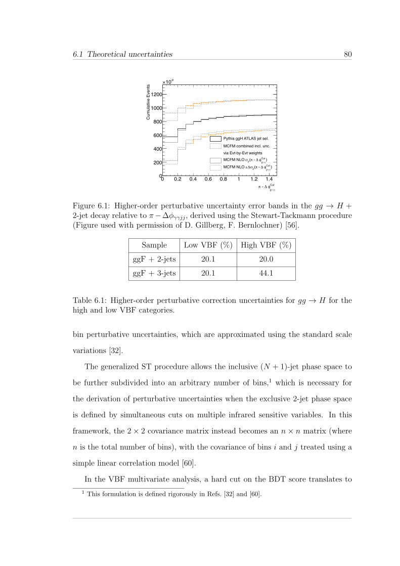
6.1 Theoretical uncertainties 80
Cut
!!jj-" # - $
0 0.2 0.4 0.6 0.8 1 1.2 1.4
Cum
ula
tive E
vents
0
200
400
600
800
1000
1200
310%
Pythia ggH ATLAS jet sel.
MCFM combined incl. unc.
via Evt-by-Evt weights
)Cut
!!jj-" # - $(
2&MCFM NLO
)Cut
!!jj-" # - $(
2&#±MCFM NLO
Figure 6.1: Higher-order perturbative uncertainty error bands in the gg → H +2-jet decay relative to π−∆φγγjj, derived using the Stewart-Tackmann procedure(Figure used with permission of D. Gillberg, F. Bernlochner) [56].
Sample Low VBF (%) High VBF (%)
ggF + 2-jets 20.1 20.0
ggF + 3-jets 20.1 44.1
Table 6.1: Higher-order perturbative correction uncertainties for gg → H for thehigh and low VBF categories.
bin perturbative uncertainties, which are approximated using the standard scale
variations [32].
The generalized ST procedure allows the inclusive (N + 1)-jet phase space to
be further subdivided into an arbitrary number of bins,1 which is necessary for
the derivation of perturbative uncertainties when the exclusive 2-jet phase space
is defined by simultaneous cuts on multiple infrared sensitive variables. In this
framework, the 2× 2 covariance matrix instead becomes an n× n matrix (where
n is the total number of bins), with the covariance of bins i and j treated using a
simple linear correlation model [60].
In the VBF multivariate analysis, a hard cut on the BDT score translates to
1 This formulation is defined rigorously in Refs. [32] and [60].
6.1 Theoretical uncertainties 81
a nonlinear, tight selection in ∆φγγjj phase space [60]. Consequently, the gg →
H + 2 jets sample is divided into exclusive 2-jet and inclusive 3-jet bins, with the
former bin composed of events passing the score threshold, and all others relegated
to the inclusive 3-jet bin. Because ∆φγγjj was the only infrared sensitive variable
used in the BDT, it was possible to apply the ST method for ∆φγγjj to compute the
perturbative uncertainties for dijet gg → H events in the VBF MVA categories.
Specifically, after applying the categorization via BDT score cuts (hence, creating
2- and ≥ 3-jet bins), the modelled ST covariance matrix was built using scale
variation uncertainties from the ≥ 2- and ≥ 3-jet bins, thereby allowing for the
derivation of ∆2 and ∆≥3. This procedure was performed for both the high and
low VBF categories, with the exclusive 2-jet bin error bands in ∆φγγjj appearing
similar to those in Figure 6.1. The resultant exclusive 2-jet and inclusive 3-jet
perturbative uncertainties for each VBF category, expressed as a fraction of the
nominal dijet yield, are given in Table 6.1.
6.1.2 Modelling uncertainties of ηZeppγγ
One particular issue that arises when using Monte Carlo samples to form an anal-
ysis is the potential for disagreement in the shapes of discriminating variables at
parton- or truth-level between Monte Carlo generators. These disparities may
arise due to the usage of different approximations, or calculations being made at
different orders (e.g. leading order vs. NLO). Therefore, beyond just looking at
reconstruction-level comparisons between Monte Carlo and data, lower-level dif-
ferences between generators must also be considered, which can be mitigated by
way of event weights and/or systematic uncertainties.
In this analysis, it was found that the distribution of the diphoton Zeppenfeld
variable (ηZeppγγ ) for gg → H + 2 jets events in Powheg disagreed with MCFM [61]
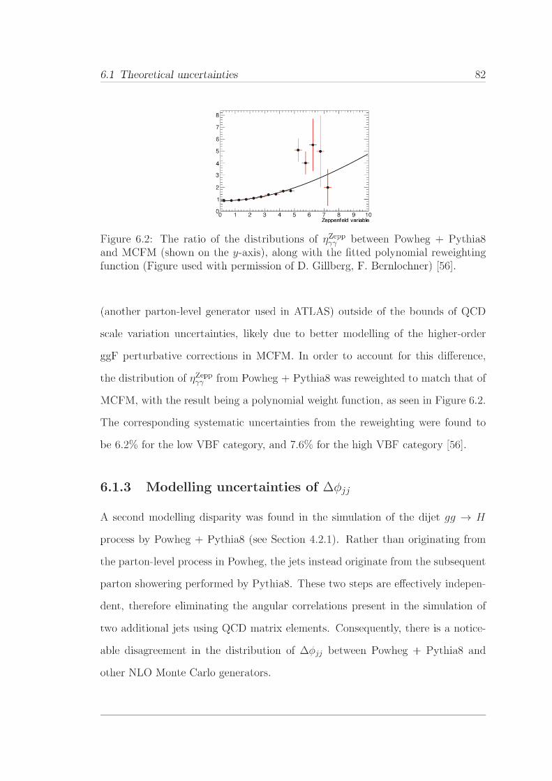
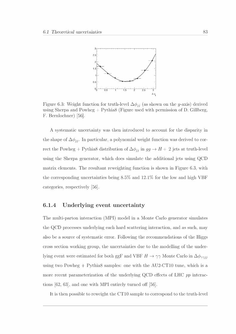
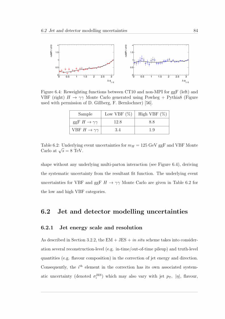
6.2 Jet and detector modelling uncertainties 84
-jj!!" #
0 0.5 1 1.5 2 2.5 3
noM
PI
/ ct1
0
0
0.5
1
1.5
2
-jj!!" #
0 0.5 1 1.5 2 2.5 3
noM
PI
/ ct1
0
0
0.5
1
1.5
2
Figure 6.4: Reweighting functions between CT10 and non-MPI for ggF (left) andVBF (right) H → γγ Monte Carlo generated using Powheg + Pythia8 (Figureused with permission of D. Gillberg, F. Bernlochner) [56].
Sample Low VBF (%) High VBF (%)
ggF H → γγ 12.8 8.8
VBF H → γγ 3.4 1.9
Table 6.2: Underlying event uncertainties for mH = 125 GeV ggF and VBF MonteCarlo at
√s = 8 TeV.
shape without any underlying multi-parton interaction (see Figure 6.4), deriving
the systematic uncertainty from the resultant fit function. The underlying event
uncertainties for VBF and ggF H → γγ Monte Carlo are given in Table 6.2 for
the low and high VBF categories.
6.2 Jet and detector modelling uncertainties
6.2.1 Jet energy scale and resolution
As described in Section 3.2.2, the EM + JES + in situ scheme takes into consider-
ation several reconstruction-level (e.g. in-time/out-of-time pileup) and truth-level
quantities (e.g. flavour composition) in the correction of jet energy and direction.
Consequently, the ith element in the correction has its own associated system-
atic uncertainty (denoted σJESi ) which may also vary with jet pT, |η|, flavour,
6.2 Jet and detector modelling uncertainties 85
etc. Therefore, it is necessary to propagate the largest of these JES uncertainties
through the rest of the statistical analysis. One propagates a given uncertainty
σJESi by producing two separate samples: a sample with all jet energies scaled
by a factor (1 + σJESi ), and another with all jet energies scaled by (1 − σJES
i ).
The average difference in dijet event yield between each shifted sample and the
nominal sample (in % of the nominal yield) becomes the JES uncertainty for that
component.
The average, non-negligible contributions to the JES uncertainty for both VBF
and ggF H → γγ Monte Carlo (mH = 125 GeV), as divided into low and high
VBF, and inclusive categories, are found in Table 6.3. Worth noting is that the
sign of each uncertainty is based on the size of the (1 + σ) dijet yield relative to
the nominal sample (i.e. ‘+’ means a greater yield, ‘−’ a smaller yield).
Another uncertainty related to jet and detector modelling is derived from the
observed differences in experimental and simulated jet energy resolution (JER) [64].
Similar to the evaluation of JES uncertainties, one propagates the JER uncertainty
by applying a smearing factor (1+σJER) to the energy of every jet, with the uncer-
tainty derived from the average difference in dijet event yield between the nominal
and smeared samples. Table 6.4 shows the resultant JER uncertainties for VBF,
ggF H → γγ Monte Carlo samples at√s = 8 TeV .
6.2.2 Jet vertex fraction selection
The jet vertex fraction, as described in Section 3.2.3, has its own associated un-
certainty, owing to the fact that a single cut is used across the entire pT and |η|
range. Since the JV F is a measure of the probability that a jet emerged from a
hard scattering interaction in a given event, one can evaluate a systematic uncer-
tainty based on JV F by varying the cut (nominally |JV F | > 0.25) by some factor,
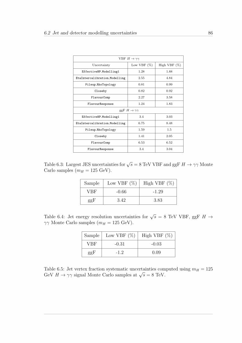
6.2 Jet and detector modelling uncertainties 86
VBF H → γγ
Uncertainty Low VBF (%) High VBF (%)
EffectiveNP Modelling1 1.28 1.88
EtaIntercalibration Modelling 2.55 4.84
Pileup RhoTopology 0.81 0.99
Closeby 0.82 0.92
FlavourComp 2.27 3.58
FlavourResponse 1.24 1.83
ggF H → γγ
EffectiveNP Modelling1 3.4 3.03
EtaIntercalibration Modelling 6.75 8.48
Pileup RhoTopology 1.59 1.5
Closeby 1.41 2.05
FlavourComp 6.53 6.52
FlavourResponse 3.4 3.04
Table 6.3: Largest JES uncertainties for√s = 8 TeV VBF and ggFH → γγ Monte
Carlo samples (mH = 125 GeV).
Sample Low VBF (%) High VBF (%)
VBF -0.66 -1.29
ggF 3.42 3.83
Table 6.4: Jet energy resolution uncertainties for√s = 8 TeV VBF, ggF H →
γγ Monte Carlo samples (mH = 125 GeV).
Sample Low VBF (%) High VBF (%)
VBF -0.31 -0.03
ggF -1.2 0.09
Table 6.5: Jet vertex fraction systematic uncertainties computed using mH = 125GeV H → γγ signal Monte Carlo samples at
√s = 8 TeV.
6.2 Jet and detector modelling uncertainties 87
and examining the difference in the dijet yield relative to the nominal sample.
The systematic shift is applied only for jets with pT < 50 GeV and |η| < 2.4,
the region which is known to be most affected by pileup jets. Jets are classified
as ‘pileup’ or ‘hard scatter’ by way of matching reconstructed jets in (y, φ) with
a corresponding truth jet,2 such that shifts are calculated for the pileup and hard
scatter jet subsets separately. The uncertainty is then derived by comparing the
yields in Monte Carlo and data for some control region using the nominal JV F cut
(denoted JV F 0). One then attempts to find looser and tighter cuts on the JV F
in Monte Carlo (denoted JV F− and JV F+, respectively) that produce the same
change in yield between the Monte Carlo sample using the nominal cut (JV F 0),
and the shifted Monte Carlo samples with cuts on JV F− and JV F+ [65].
For example, if a nominal cut of |JV F | > 0.25 ≡ JV F 0 shows a 5% difference
in yield between the Monte Carlo and data samples, one would look for cuts
|JV F | > JV F+ and |JV F | > JV F− that produce a∼ 5% change in yield between
the nominal Monte Carlo sample, and the Monte Carlo samples with the shifted
cuts. By running the analysis thrice – alternately requiring |JV F | > JV F 0, then
|JV F | > JV F+, and finally |JV F | > JV F− – one obtains the uncertainty from
the average difference in dijet yield between the nominal and shifted samples.
For the VBF multivariate analysis, the JV F -based systematic uncertainties were
evaluated for VBF and ggF H → γγ Monte Carlo (mH = 125 GeV), as shown in
Table 6.5.
2 Here, y is the rapidity, y = 12ln
(
E+pL
E−pL
)
. Each truth jet is also required to have pTruthT > 10
GeV.
Chapter 7
VBF multivariate analysis results
After the BDT-based VBF H → γγ categorization was built and optimized, the
final test of the analysis was the application to the full, unblinded 2011 and 2012
data sets, constituting ∼ 7 fb−1 of√s = 7TeV pp collisions, and ∼ 21 fb−1
of√s = 8TeV pp collisions, respectively. The events selected using the BDT
categorization underwent statistical tests to search for evidence (or perhaps the
discovery) of a VBF-mediated H → γγ-like process, and quantify the observed
amount of signal relative to Standard Model predictions.
7.1 Analysis goals
With the discovery of a Standard Model Higgs boson-like particle claimed mid-
way through 2012, the goal of the final analysis was to update the results of the
statistical tests that led to the initial discovery. In doing so, it was possible to
re-examine and validate the previous results from the VBF H → γγ channel
using both greater statistics, and improved signal discrimination by way of the
new BDT-based categorization. These tasks were performed by calculating two
statistical quantities:
88
7.1 Analysis goals 89
• Signal strength and error, µ ± δµ, where µ = σ/σSM – For a given
signal process, µ is defined as the ratio between the observed cross section
and the Standard Model prediction at a Higgs boson mass mH . The signal
strength effectively quantifies how the signal rate behaves relative to what
is expected of the Standard Model under the same conditions [66]. In this
framework, µ = 0 corresponds to no signal (i.e. background only), while
µ = 1 implies perfect agreement with Standard Model predictions. Given
that the cross sectional measurements are fixed to what is observed using
the ATLAS detector, the main goal is the minimization of δµ, which will put
a hard limit on whether the observed signal rate agrees with the Standard
Model, or indicates new physics, i.e. µ deviating from 1, beyond the limits
of statistical and systematic error.
• p-value for background-only hypothesis, p0 – The quantity p0 is rep-
resentative of the level of disagreement between recorded data and the
background-only hypothesis, and is found by integrating the PDF of the
maximum likelihood test statistic q0 (see Equation 7.4). This p-value is
used to quantify particle discovery, such that a smaller p0 implies a greater
probability that a signal-like resonance has been observed.
In practice, the best fit signal strengths for each production channel are found by
way of a profile likelihood ratio which depends on the Higgs boson mass mH , and
a series of nuisance parameters θ (i.e. systematic uncertainties) [57],
λ(µ) =L(µ, ˆθ)
L(µ, θ). (7.1)
The likelihood function L(µ,θ) for a given channel originates in the idea of experi-
mental data being represented as an N -bin histogram,1 defined as n = (n1, ..., nN),
1 Typically, the likelihood is formed using a binned distribution of mγγ .
7.1 Analysis goals 90
with another M -bin histogram used to constrain nuisance parameters. The resul-
tant function is then given by the product of the Poisson probabilities for each
bin [57],
L(µ,θ) =N∏
j=1
(µsj + bj)nj
nj!e−(µsj+bj)
M∏
k=1
umk
k
mk!e−uk . (7.2)
where sj and bj are the mean number of entries in bin nj for signal and back-
ground (respectively), and ui(θ) = E[mi] is the expectation value of bin mi from
the M -bin histogram. Here, the single circumflex denotes the unconditional max-
imum likelihood estimate of a parameter, and the double circumflex denotes the
conditional maximum likelihood estimate for a fixed µ [66]. For a given Higgs
boson production process observable through ATLAS, the cross section is given
by [15],
σH =NS+B − 〈NB〉ǫ∫
L dt. (7.3)
Here, NS+B is the combined signal + background rate, 〈NB〉 is the expected number
of background events derived from fitted data, ǫ is the product of various efficiency
factors (such as detector efficiency), and∫
L dt is the integrated luminosity (in
units of fb−1).
We may use the profile likelihood ratio λ(µ) to calculate the probability of
signal discovery for a given mH under the assumption that µ ≥ 0 (i.e. a signal
process can only add to the existing background statistics). A test statistic q0 is
derived to rule out the background-only hypothesis (µ = 0) [57] as,
7.2 Training samples and BDT response 91
q0 =
−2 lnλ(0), µ ≥ 0,
0, µ < 0.
(7.4)
Accordingly, the level of disagreement between data and the background-only
hypothesis is quantified as,
p0 =
∫ ∞
q0(obs)
f(q0|0) dq0, (7.5)
where λ(0) is the profile likelihood ratio for µ = 0. When evaluating the background-
only hypothesis, the function f(q0|0) can be approximated analytically as [57],
f(q0|0) =1
2δ(q0) +
1
2
1√2π
1√q0e−q0/2. (7.6)
This expression can be integrated easily to derive the value of p0,
p0 = 1− Φ(√q0), (7.7)
with the corresponding significance being Z0 = Φ−1(1− p0) =√q0, with Φ being
the cumulative PDF of the Gaussian distribution. If Z0 > 5σ (or, equivalently, if
p0 < 2.87× 10⁻⁷), then a particle discovery is claimed for the observed signal.
7.2 Training samples and BDT response
In Figure 7.1, distributions of the BDT score are shown for the various testing sam-
ples used in the analysis. Specifically, in Figure 7.1(a), good agreement is observed
in the BDT response of the Sherpa + inverted isolation background testing sam-
ple, and the full 2012 dataset, within experimental uncertainty. Furthermore, in
Figure 7.1(b), a sharp contrast is observed between the BDT response of the VBF
Monte Carlo testing sample, and the ggF Monte Carlo and background samples.
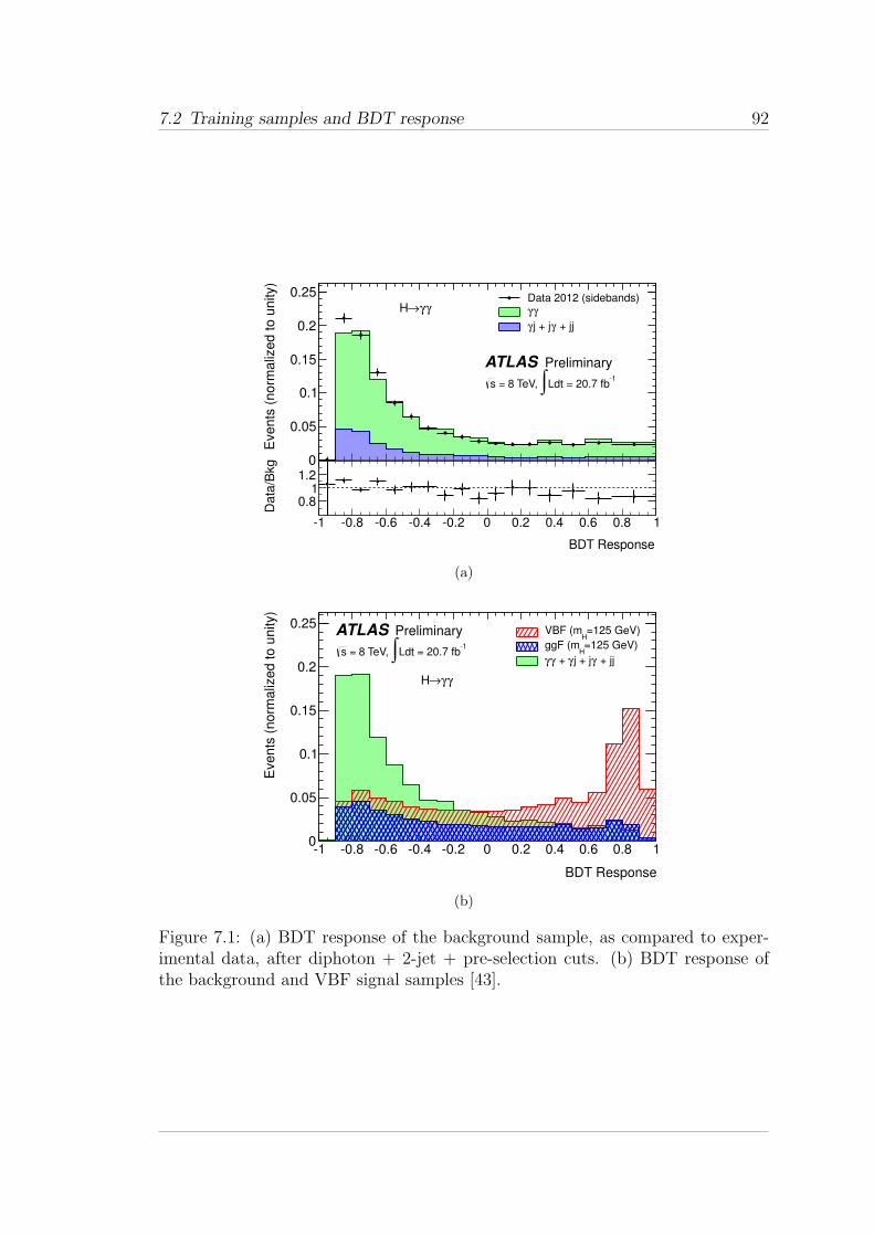
7.2 Training samples and BDT response 92
Eve
nts
(n
orm
aliz
ed
to
un
ity)
0
0.05
0.1
0.15
0.2
0.25 Data 2012 (sidebands)γγ
+ jjγj + jγ
ATLAS Preliminary-1
Ldt = 20.7 fb∫ = 8 TeV, s
γγ→H
BDT Response
-1 -0.8 -0.6 -0.4 -0.2 0 0.2 0.4 0.6 0.8 1
Data
/Bkg
0.81
1.2
(a)
BDT Response
-1 -0.8 -0.6 -0.4 -0.2 0 0.2 0.4 0.6 0.8 1
Eve
nts
(n
orm
aliz
ed
to
un
ity)
0
0.05
0.1
0.15
0.2
0.25=125 GeV)
HVBF (m
=125 GeV)H
ggF (m
+ jj γj + jγ + γγ
ATLAS Preliminary-1
Ldt = 20.7 fb∫ = 8 TeV, s
γγ→H
(b)
Figure 7.1: (a) BDT response of the background sample, as compared to exper-imental data, after diphoton + 2-jet + pre-selection cuts. (b) BDT response ofthe background and VBF signal samples [43].
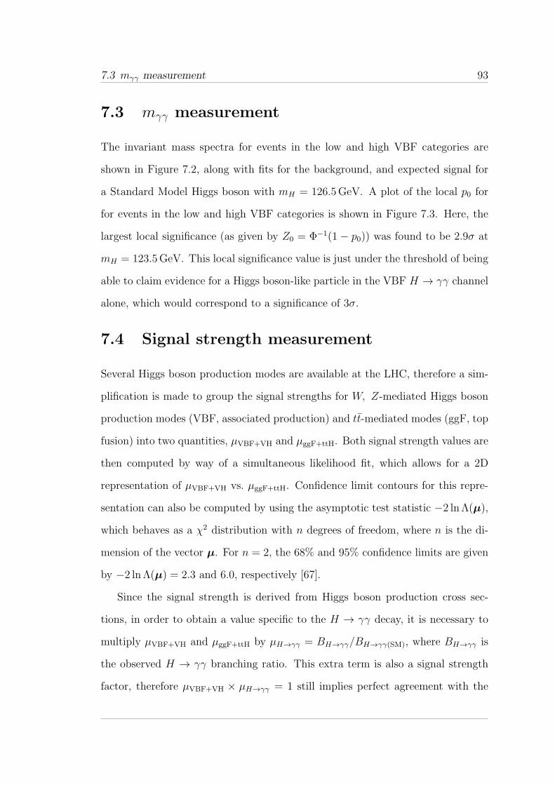
7.3 mγγ measurement 93
7.3 mγγ measurement
The invariant mass spectra for events in the low and high VBF categories are
shown in Figure 7.2, along with fits for the background, and expected signal for
a Standard Model Higgs boson with mH = 126.5GeV. A plot of the local p0 for
for events in the low and high VBF categories is shown in Figure 7.3. Here, the
largest local significance (as given by Z0 = Φ−1(1 − p0)) was found to be 2.9σ at
mH = 123.5GeV. This local significance value is just under the threshold of being
able to claim evidence for a Higgs boson-like particle in the VBF H → γγ channel
alone, which would correspond to a significance of 3σ.
7.4 Signal strength measurement
Several Higgs boson production modes are available at the LHC, therefore a sim-
plification is made to group the signal strengths for W, Z-mediated Higgs boson
production modes (VBF, associated production) and tt-mediated modes (ggF, top
fusion) into two quantities, µVBF+VH and µggF+ttH. Both signal strength values are
then computed by way of a simultaneous likelihood fit, which allows for a 2D
representation of µVBF+VH vs. µggF+ttH. Confidence limit contours for this repre-
sentation can also be computed by using the asymptotic test statistic −2 lnΛ(µ),
which behaves as a χ2 distribution with n degrees of freedom, where n is the di-
mension of the vector µ. For n = 2, the 68% and 95% confidence limits are given
by −2 lnΛ(µ) = 2.3 and 6.0, respectively [67].
Since the signal strength is derived from Higgs boson production cross sec-
tions, in order to obtain a value specific to the H → γγ decay, it is necessary to
multiply µVBF+VH and µggF+ttH by µH→γγ = BH→γγ/BH→γγ(SM), where BH→γγ is
the observed H → γγ branching ratio. This extra term is also a signal strength
factor, therefore µVBF+VH × µH→γγ = 1 still implies perfect agreement with the
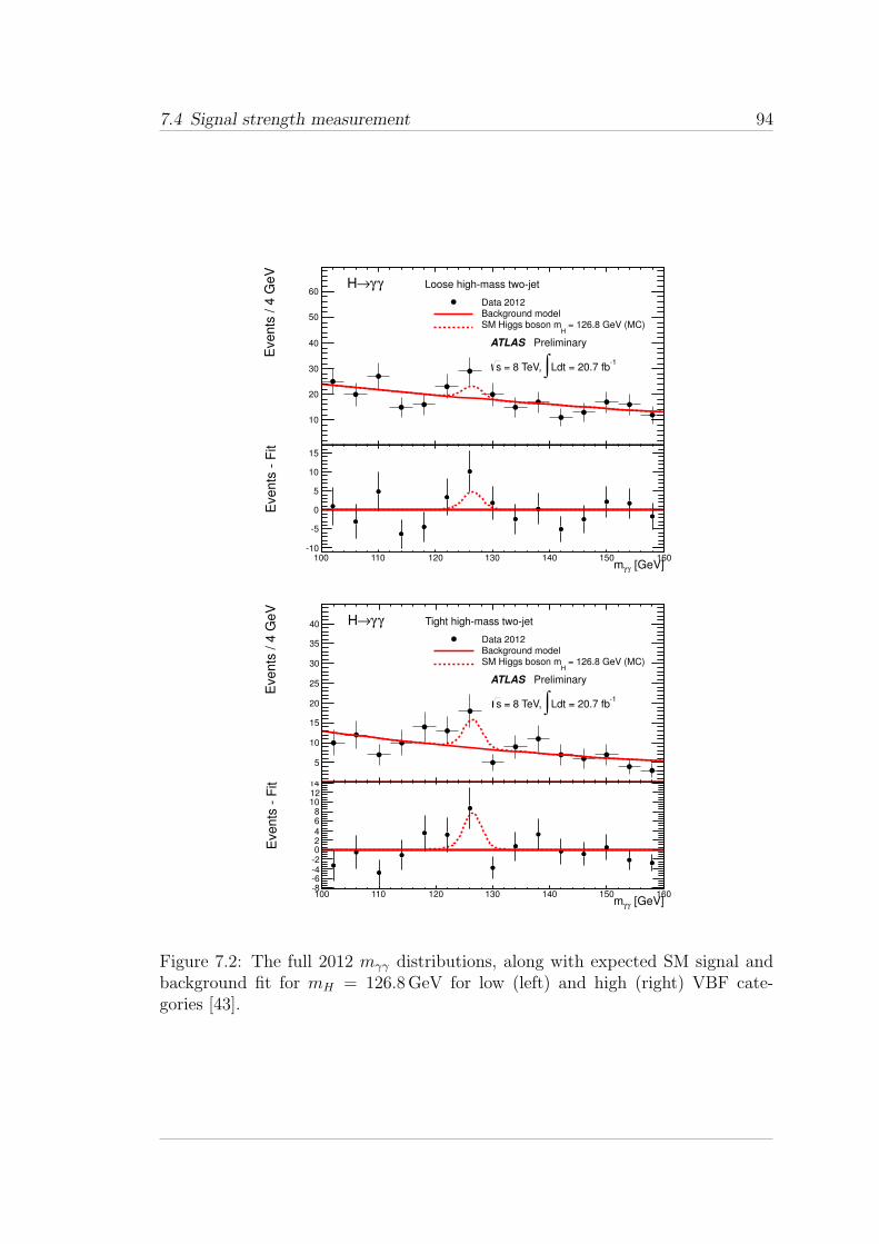
7.4 Signal strength measurement 94
Events
/ 4
GeV
10
20
30
40
50
60
ATLAS Preliminary
γγ→H
-1Ldt = 20.7 fb∫ = 8 TeV, s
Loose high-mass two-jet
Data 2012Background model
= 126.8 GeV (MC)H
SM Higgs boson m
[GeV]γγm100 110 120 130 140 150 160
Eve
nts
- F
it
-10
-5
0
5
10
15
Eve
nts
/ 4
Ge
V
5
10
15
20
25
30
35
40
ATLAS Preliminary
γγ→H
-1Ldt = 20.7 fb∫ = 8 TeV, s
Tight high-mass two-jet
Data 2012Background model
= 126.8 GeV (MC)H
SM Higgs boson m
[GeV]γγm100 110 120 130 140 150 160
Events
- F
it
-8-6-4-202468
101214
Figure 7.2: The full 2012 mγγ distributions, along with expected SM signal andbackground fit for mH = 126.8GeV for low (left) and high (right) VBF cate-gories [43].

7.4 Signal strength measurement 95
Standard Model. After performing the profile likelihood ratio maximization, the
best fit signal strength measurement for W,Z-mediated H → γγ signal was found
at a Higgs boson mass of mH = 126.8GeV to be [43],
µVBF+VH × µH→γγ = 1.72+0.85−0.77 (stat)+0.48
−0.29 (syst)+0.25−0.29 (theory),
which agrees with Standard Model predictions (given as × in Figure 7.3(b)) within
2σ, as represented by the 95% confidence limit contour.
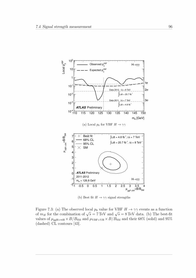
7.4 Signal strength measurement 96
[GeV]Hm
110 115 120 125 130 135 140 145 150
VB
F
0L
oca
l p
-410
-310
-210
-110
1
10
210VBF
0Observed p
VBF
0Expected p
= 8 TeVsData 2012,
-1Ldt = 20.7 fb∫
= 7 TeVsData 2011,
-1Ldt = 4.8 fb∫
ATLAS Preliminary
σ1
σ2
σ3
γγ→H
(a) Local p0 for VBF H → γγ
SMB/B×
ggF+ttHµ
-1 -0.5 0 0.5 1 1.5 2 2.5 3 3.5 4
SM
B/B
×V
BF
+V
Hµ
-2
-1
0
1
2
3
4
5
6
7
PreliminaryATLAS
2011-2012
= 126.8 GeVHm
= 7 TeVs, -1Ldt = 4.8 fb∫ = 8 TeVs, -1Ldt = 20.7 fb∫
Best fit
68% CL
95% CL
SM
γγ→H
(b) Best fit H → γγ signal strengths
Figure 7.3: (a) The observed local p0 value for VBF H → γγ events as a functionof mH for the combination of
√s = 7TeV and
√s = 8TeV data. (b) The best-fit
values of µggH+ttH×B/BSM and µVBF+VH×B/BSM and their 68% (solid) and 95%(dashed) CL contours [43].
Chapter 8
Conclusions
The kinematically unique properties of the vector boson fusion production mech-
anism allow for a multitude of methods to isolate Higgs boson-like signal, with
varying degrees of success. When coupled with the distinct kinematics and heav-
ily reducible backgrounds of the H → γγ process, it becomes possible to search
for both direct evidence of Higgs boson production, as well as quantify its rate of
production relative to Standard Model predictions. It has been shown that the
isolation of signal resembling VBF H → γγ is possible (and indeed, quite suc-
cessful) using a multivariate analysis approach – specifically, through the use of a
boosted decision tree, developed using orthogonal signal and background samples.
A primary iteration of the VBF multivariate analysis was derived using a BDT
trained on inverted isolation background and VBF H → γγ signal Monte Carlo
samples. It was found that the variables contributing the most discriminating
power related to the dijet mass, jet pseudorapidity separation, and balance of the
dijet + diphoton system. A second iteration of the analysis was then performed,
with the goal of improving signal discrimination through better background mod-
elling and variable selection. It was found that the irreducible γγ and γj+ jγ+ jj
components of the H → γγ background were modeled reasonably well by the com-
bination of a Sherpa γγ Monte Carlo sample and inverted isolation diphoton data,
97
98
weighted to the approximate proportions of true and fake diphoton components,
respectively, of the H → γγ background. Evidence of this similarity was found in
the agreement of the BDT score distributions of the γγ data sidebands and back-
ground model, as well as the agreement in the resultant kinematic distributions
after performing VBF categorization via cuts on the event-by-event BDT score.
A final statistical analysis was performed on the full 2011 − 2012 dataset to
quantify the discovery significance and signal strength of signal resembling the
VBF-mediated H → γγ decay. The resultant discovery significance was found
to be Z0 = 2.9σ at an invariant mass of mH = 123.5 GeV. In combining the
results of the VBF categorization with those of the associated production-enriched
categories, the best-fit signal strength for W, Z-mediated Higgs boson production
was found to be µVBF+VH × B/BSM = 1.72 at an invariant mass of mH = 126.8
GeV, which agrees with Standard Model production rates within 2σ.
Ongoing work involving multivariate analysis techniques in the H → γγ chan-
nel includes the implementation of two-dimensional BDTs, the refinement of signal
and background samples, and the application of the boosted decision tree method
to other facets of the H → γγ analysis (e.g. spin studies). The same type of
machinery is also being extended to other VBF-mediated Higgs boson decays,
such as H → ZZ∗ → 4l. One practical consideration for the extension of this
method is the rate of VBF production for a given decay process. For example,
VBF-mediated H → ZZ∗ → 4l is an exceptionally rare process, necessitating
much larger volumes of data to ensure the practicality of a multivariate analysis.
However, with the planned resumption of collisions and data taking in 2015 at
full design luminosity and centre-of-mass energy, the prospect of discovering and
studying additional VBF-mediated Higgs boson decays using multivariate analysis
techniques looks increasingly bright.
References
[1] Particle Data Group, Review of Particle Physics , Phys. Rev. D 86 (2012)
010001.
[2] Super-Kamiokande Collaboration, Y. Fukuda et al., Evidence for oscillation
of atmospheric neutrinos , Phys. Rev. Lett. 81 (1998) 1562–1567,
arXiv:hep-ex/9807003 [hep-ex].
[3] SNO Collaboration, B. Aharmim et al., Electron energy spectra, fluxes, and
day-night asymmetries of B-8 solar neutrinos from measurements with NaCl
dissolved in the heavy-water detector at the Sudbury Neutrino Observatory ,
Phys. Rev. C72 (2005) 055502, arXiv:nucl-ex/0502021 [nucl-ex].
[4] J. Goldstone, Field theories with superconductor solutions , Nuovo Cimento
19 (1960) no. CERN-TH-118, 154–164.
[5] E. Fermi, Tentativo di una Teoria dei Raggi β, Il Nuovo Cimento 11 (1934)
no. 1, 1–19.
[6] P.W. Higgs, Broken symmetries, massless particles and gauge fields , Phys.
Lett. 12 (1964) 132–133.
[7] F. Englert and R. Brout, Broken symmetry and the mass of gauge vector
mesons , Phys. Rev. Lett 13 (1964) 321–323.
99
REFERENCES 100
[8] G. Guralnik, C. Hagen and T. Kibble, Global conservation laws and
massless particles , Phys. Rev. Lett. 13 (1964) 585–587.
[9] ATLAS Collaboration, Expected photon performance in the ATLAS
experiment , ATL-PHYS-PUB-2011-007, CERN, Geneva, Apr, 2011.
[10] ATLAS Collaboration, The ATLAS Experiment at the CERN Large Hadron
Collider , Journal of Instrumentation 3 (2008) no. 08, S08003.
[11] D. Green, Vector boson fusion Higgs production at the LHC: Mass variables ,
arXiv:hep-ex/0501027 [hep-ex].
[12] LHC Higgs Cross Section Working Group, Handbook of LHC Higgs Cross
Sections: 1. Inclusive Observables , arXiv:1101.0593 [hep-ph].
[13] R. Tanaka, C. Mariotti, S. Heinemeyer, and G. Passarino, LHC Higgs Cross
Section Working Group,
https://twiki.cern.ch/twiki/bin/view/LHCPhysics/CrossSections,
All figures used with permission of LHC HXSWG, May, 2013.
[14] ATLAS Collaboration, Observation of a new particle in the search for the
Standard Model Higgs boson with the ATLAS detector at the LHC , Phys.
Lett. B716 (2012) 1–29, arXiv:1207.7214 [hep-ex].
[15] D. Zeppenfeld, R. Kinnunen, A. Nikitenko, and E. Richter-Was, Measuring
Higgs boson couplings at the CERN LHC , Phys. Rev. D62 (2000) 013009,
arXiv:hep-ph/0002036 [hep-ph].
[16] The HSG1 Group, Selection for H → γγ analysis supporting note, for
Moriond 2013 , ATL-COM-PHYS-2013-093, CERN, Geneva, Jan, 2013.
REFERENCES 101
[17] ATLAS Collaboration, Performance of the Reconstruction and Identification
of Hadronic Tau Decays with ATLAS , ATLAS-CONF-2011-152, CERN,
Geneva, Nov, 2011.
[18] R. Fernow, Introduction to Experimental Particle Physics. Cambridge
University Press, Cambridge, England, 1986.
[19] A. Djouadi, The anatomy of electroweak symmetry breaking: Tome I: The
Higgs boson in the Standard Model , Physics Reports 457 (2008) no. 1 - 4, 1
– 216.
[20] D.L. Rainwater, Intermediate-Mass Higgs Searches in Weak Boson Fusion.
PhD thesis, University of Wisconsin-Madison, 2008.
[21] M. Spira, QCD effects in Higgs physics , Fortsch. Phys. 46 (1998) 203–284,
arXiv:hep-ph/9705337 [hep-ph].
[22] P. Bolzoni, F. Maltoni, S. Moch, and M. Zaro, Higgs production via
vector-boson fusion at NNLO in QCD , Phys. Rev. Lett. 105 (2010) 011801,
arXiv:1003.4451 [hep-ph].
[23] T. Han, G. Valencia, and S. Willenbrock, Structure function approach to
vector boson scattering in pp collisions , Phys. Rev. Lett. 69 (1992)
3274–3277.
[24] G. Degrassi and F. Maltoni, Two-loop electroweak corrections to the
Higgs-boson decay H → γγ, Nucl. Phys. B724 (2005) 183–196,
arXiv:hep-ph/0504137 [hep-ph].
[25] U. Aglietti, R. Bonciani, G. Degrassi, and A. Vicini, Two loop light fermion
contribution to Higgs production and decays , Phys. Lett. B595 (2004)
432–441, arXiv:hep-ph/0404071 [hep-ph].
REFERENCES 102
[26] U. Aglietti, R. Bonciani, G. Degrassi, and A. Vicini, Master integrals for the
two-loop light fermion contributions to gg → H and H → γγ, Phys. Lett.
B600 (2004) 57–64, arXiv:hep-ph/0407162 [hep-ph].
[27] A. Djouadi, M. Spira, J. van der Bij, and P. Zerwas, QCD corrections to
gamma gamma decays of Higgs particles in the intermediate mass range,
Phys. Lett. B257 (1991) 187–190.
[28] K. Melnikov and O. I. Yakovlev, Higgs → two photon decay: QCD radiative
correction, Phys. Lett. B312 (1993) 179–183, arXiv:hep-ph/9302281
[hep-ph].
[29] S. Frixione, P. Nason, and C. Oleari, Matching NLO QCD computations
with Parton Shower simulations: the POWHEG method , JHEP 0711 (2007)
070, arXiv:0709.2092 [hep-ph].
[30] S. Alioli, P. Nason, C. Oleari, and E. Re, A general framework for
implementing NLO calculations in shower Monte Carlo programs: the
POWHEG BOX , JHEP 1006 (2010) 043, arXiv:1002.2581 [hep-ph].
[31] ATLAS Collaboration, Expected Performance of the ATLAS Experiment -
Detector, Trigger and Physics , CERN-OPEN-2008-020 (2009) ,
arXiv:0901.0512 [hep-ex].
[32] S. Gangal and F. J. Tackmann, Next-to-leading-order uncertainties in
Higgs+ 2 jets from gluon fusion, Phys. Rev. D 87 (2013) 093008.
[33] U. Egede, The search for a standard model Higgs at the LHC and electron
identification using transition radiation in the ATLAS tracker. PhD thesis,
Lund University, 1998.
REFERENCES 103
[34] LHC Higgs Cross Section Working Group, Handbook of LHC Higgs Cross
Sections: 2. Differential Distributions , arXiv:1201.3084 [hep-ph].
[35] T. Sjostrand, S. Mrenna, and P. Z. Skands, A Brief Introduction to
PYTHIA 8.1 , Comput. Phys. Commun. 178 (2008) 852–867,
arXiv:0710.3820 [hep-ph].
[36] W. Lampl, S. Laplace, D. Lelas, P. Loch, H. Ma, S. Menke, S. Rajagopalan,
D. Rousseau, S. Snyder, and G. Unal, Calorimeter Clustering Algorithms:
Description and Performance, ATL-LARG-PUB-2008-002.
ATL-COM-LARG-2008-003, CERN, Geneva, Apr, 2008.
[37] ATLAS Collaboration, F. Hirsch, Tracking and vertexing with the ATLAS
detector at the LHC , Nucl. Instrum. Meth. in Phys. Res. A650 (2011)
218–223.
[38] F. Balli, C. Sawyer, M. Scherzer, M. Swiatlowski, J. Backus Mayes,
A. Schwartzman, S. Menke, J. Stahlman, and S. Sacerdoti, The Effects of
Pile-up and Noise Thresholds on Jet and EmissT Performance in the ATLAS
detector , ATL-COM-PHYS-2013-008, CERN, Geneva, Jan, 2012.
[39] M. Cacciari and G. P. Salam, The anti-kt jet clustering algorithm, JHEP
2008 (2008) no. 04, 1 – 12.
[40] S. Argyropoulos, J. A. Backus Mayes, L. Bryngemark, R. C. Camacho Toro,
J. Katzy, J. Lacey, C. Sawyer, A. Schwartzman, and P. Starovoitov, Pile-up
subtraction and suppression for jets in ATLAS , ATL-COM-PHYS-2013-251,
CERN, Geneva, Mar, 2013.
REFERENCES 104
[41] D. W. Miller, A. Schwartzman, and D. Su, Pile-up jet energy scale
corrections using the jet-vertex fraction method , ATL-PHYS-INT-2009-090,
CERN, Geneva, Sep, 2009.
[42] ATLAS Collaboration, Jet energy measurement with the ATLAS detector in
proton-proton collisions at√s = 7 TeV, Eur. Phys. J. C73 (2013) no. 3,
1–118.
[43] ATLAS Collaboration, Measurements of the properties of the Higgs-like
boson in the two photon decay channel with the ATLAS detector using 25
fb−1 of proton-proton collision data, ATLAS-CONF-2013-012, CERN,
Geneva, Mar, 2013.
[44] ATLAS Collaboration, Search for the Standard Model Higgs boson in the
diphoton decay channel with 4.9 fb−1 of pp collisions at√s = 7 TeV with
ATLAS , Phys. Rev. Lett. 108 (2012) 111803, arXiv:1202.1414 [hep-ex].
[45] OPAL Collaboration, G. Abbiendi et al., Search for anomalous production
of dilepton events with missing transverse momentum in e+e− collisions at
√s = 183 GeV to 209 GeV , Eur. Phys. J. C32 (2004) 453–473,
arXiv:hep-ex/0309014 [hep-ex].
[46] M. Vesterinen and T. Wyatt, A Novel Technique for Studying the Z Boson
Transverse Momentum Distribution at Hadron Colliders , Nucl. Instrum.
Meth. in Phys. Res. A602 (2009) 432–437, arXiv:0807.4956 [hep-ex].
[47] A. Hoecker, P. Speckmayer, J. Stelzer, J. Therhaag, E. von Toerne, H. Voss,
et al., TMVA: Toolkit for Multivariate Data Analysis , Proceedings of
Science ACAT (2007) 040, arXiv:physics/0703039.
REFERENCES 105
[48] J. Friedman, Stochastic gradient boosting , Computational Statistics & Data
Analysis 38 (2002) no. 4, 367 – 378.
[49] J. Allison, K. Amako, J. Apostolakis, H. Araujo, P. Dubois, et al., GEANT4
developments and applications , IEEE Trans. Nucl. Sci. 53 (2006) 270–278.
[50] GEANT4 Collaboration, S. Agostinelli et al., GEANT4: A Simulation
toolkit , Nucl. Instrum. Meth. in Phys. Res. A506 (2003) 250–303.
[51] ATLAS Collaboration, ATLAS detector and physics performance: Technical
Design Report. CERN, Geneva, 1999.
[52] T. Gleisberg, S. Hoeche, F. Krauss, A. Schalicke, S. Schumann, et al.,
SHERPA 1. alpha: A Proof of concept version, JHEP 0402 (2004) 056,
arXiv:hep-ph/0311263 [hep-ph].
[53] T. Gleisberg, S. Hoeche, F. Krauss, M. Schonherr, S. Schumann, et al.,
Event generation with SHERPA 1.1 , JHEP 0902 (2009) 007,
arXiv:0811.4622 [hep-ph].
[54] L. J. Dixon and M. S. Siu, Resonance continuum interference in the
diphoton Higgs signal at the LHC , Phys. Rev. Lett. 90 (2003) 252001,
arXiv:hep-ph/0302233 [hep-ph].
[55] ATLAS Collaboration, Search for the Standard Model Higgs boson in the
diphoton decay channel with 4.9 fb−1 of ATLAS data at√s = 7 TeV ,
ATLAS-CONF-2011-161, CERN, Geneva, Dec, 2011.
[56] The HSG1 Group, Multivariate analysis for the search of VBF Higgs to
gamma gamma, ATL-COM-PHYS-2013-076, CERN, Geneva, Jan, 2013.
REFERENCES 106
[57] G. Cowan, K. Cranmer, E. Gross, and O. Vitells, Asymptotic formulae for
likelihood-based tests of new physics , Eur. Phys. J. C71 (2011) 1554, 1–19,
arXiv:1007.1727 [physics.data-an].
[58] ATLAS Collaboration, Observation and study of the Higgs boson candidate
in the two photon decay channel with the ATLAS detector at the LHC ,
ATLAS-CONF-2012-168, CERN, Geneva, Dec, 2012.
[59] I. W. Stewart and F. J. Tackmann, Theory Uncertainties for Higgs and
Other Searches Using Jet Bins , Phys. Rev. D85 (2012) 034011,
arXiv:1107.2117 [hep-ph].
[60] LHC Higgs Cross Section Working Group, Handbook of LHC Higgs Cross
Sections: 3. Higgs Properties , arXiv:1307.1347 [hep-ph].
[61] J. M. Campbell and R. Ellis, MCFM for the Tevatron and the LHC , Nucl.
Phys. Proc. Suppl. 205-206 (2010) 10–15, arXiv:1007.3492 [hep-ph].
[62] M. Guzzi, P. Nadolsky, E. Berger, H.-L. Lai, F. Olness, et al., CT10 parton
distributions and other developments in the global QCD analysis ,
arXiv:1101.0561 [hep-ph].
[63] ATLAS Collaboration, Summary of ATLAS Pythia 8 tunes ,
ATL-PHYS-PUB-2012-003, CERN, Geneva, Aug, 2012.
[64] ATLAS Collaboration, Jet energy resolution in proton-proton collisions at
√s = 7 TeV recorded in 2010 with the ATLAS detector , Eur. Phys. J. C73
(2013) 2306, 1–118, arXiv:1210.6210 [hep-ex].
[65] R. Camacho Toro, Jet Vertex Fraction (JVF) status , Presented at
Jet/Etmiss phone meeting, Jan, 2013.
REFERENCES 107
[66] ATLAS Collaboration, An update of combined measurements of the new
Higgs-like boson with high mass resolution channels ,
ATLAS-CONF-2012-170, CERN, Geneva, 2012.
[67] ATLAS Collaboration, Combined coupling measurements of the Higgs-like
boson with the ATLAS detector using up to 25 fb−1 of proton-proton
collision data, ATLAS-CONF-2013-034, CERN, Geneva, Mar, 2013.
[68] Teresa Barillari (on behalf of the ATLAS Collaboration), Jet Energy Scale
Uncertainties in ATLAS , Journal of Physics: Conference Series 404 (2012)
no. 1, 012012.
[69] ATLAS Collaboration, JES flavour uncertainty studies ,
https://twiki.cern.ch/twiki/bin/viewauth/AtlasProtected/
JESFlavourUncertaintyStudies, Jun, 2013.
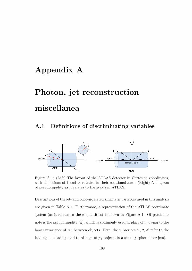
Appendix A
Photon, jet reconstruction
miscellanea
A.1 Definitions of discriminating variables
Figure A.1: (Left) The layout of the ATLAS detector in Cartesian coordinates,with definitions of θ and φ, relative to their rotational axes. (Right) A diagramof pseudorapidity as it relates to the z-axis in ATLAS.
Descriptions of the jet- and photon-related kinematic variables used in this analysis
are given in Table A.1. Furthermore, a representation of the ATLAS coordinate
system (as it relates to these quantities) is shown in Figure A.1. Of particular
note is the pseudorapidity (η), which is commonly used in place of θ, owing to the
boost invariance of ∆η between objects. Here, the subscripts ‘1, 2, 3’ refer to the
leading, subleading, and third-highest pT objects in a set (e.g. photons or jets).
108
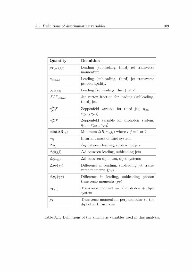
A.1 Definitions of discriminating variables 109
Quantity Definition
pT(jet1,2,3) Leading (subleading, third) jet transversemomentum.
ηjet1,2,3 Leading (subleading, third) jet transversepseudorapidity.
φjet1,2,3 Leading (subleading, third) jet φ.
JV Fjet1,2,3 Jet vertex fraction for leading (subleading,third) jet.
ηZeppjet3 Zeppenfeld variable for third jet, ηjet3 −〈ηjet1, ηjet2〉
ηZeppγγ Zeppenfeld variable for diphoton system,ηγγ − 〈ηjet1, ηjet2〉
min(∆Rjγ) Minimum ∆R(γi, jj) where i, j = 1 or 2
mjj Invariant mass of dijet system
∆ηjj ∆η between leading, subleading jets
∆φ(jj) ∆φ between leading, subleading jets
∆φγγjj ∆φ between diphoton, dijet systems
∆pT(jj) Difference in leading, subleading jet trans-verse momenta (pT)
∆pT(γγ) Difference in leading, subleading photontransverse momenta (pT)
pTγγjj Transverse momentum of diphoton + dijetsystem
pTt Transverse momentum perpendicular to thediphoton thrust axis
Table A.1: Definitions of the kinematic variables used in this analysis.
A.2 Comparison of background samples after dijet selection 110
A.2 Comparison of background samples after di-
jet selection
An extensive comparison of jet- and photon-related quantities for different back-
ground samples is given in Figure A.2. Samples under consideration include in-
verted isolation data, Sherpa and Pythia γγ Monte Carlo, as well as data side-
bands, with each sample restricted to an invariant mass range 100 < mγγ <
160GeV. Below each plot, the ratio of each background model distribution to the
sideband data is shown. In terms of general agreement between jet, photon, and
dijet/diphoton variables, inverted isolation background data is the best choice to
model the data sidebands using a single, unmixed sample.
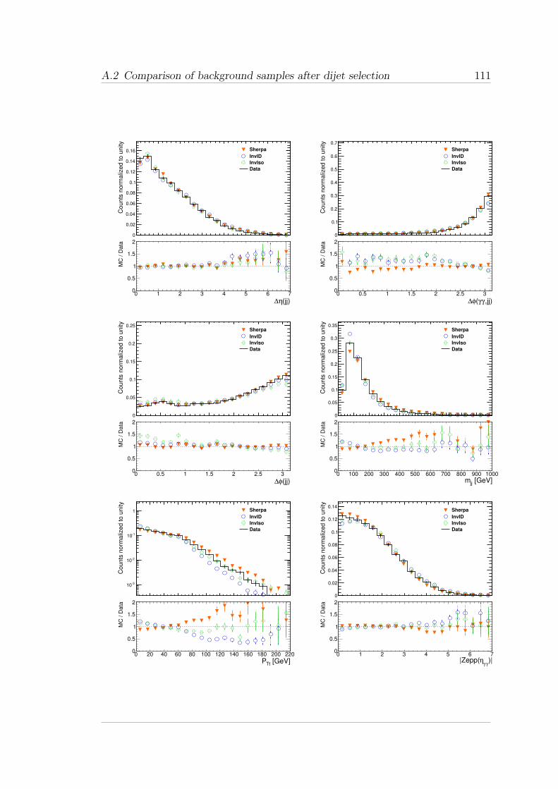
A.2 Comparison of background samples after dijet selection 111
Co
un
ts n
orm
aliz
ed
to
un
ity
0
0.02
0.04
0.06
0.08
0.1
0.12
0.14
0.16 Sherpa
InvID
InvIso
Data
(jj)η∆0 1 2 3 4 5 6 7
MC
/ D
ata
0
0.5
1
1.5
2
Co
un
ts n
orm
aliz
ed
to
un
ity
0
0.1
0.2
0.3
0.4
0.5
0.6
0.7
Sherpa
InvID
InvIso
Data
,jj)γγ(φ∆0 0.5 1 1.5 2 2.5 3
MC
/ D
ata
0
0.5
1
1.5
2
Co
un
ts n
orm
aliz
ed
to
un
ity
0
0.05
0.1
0.15
0.2
0.25Sherpa
InvID
InvIso
Data
(jj)φ∆0 0.5 1 1.5 2 2.5 3
MC
/ D
ata
0
0.5
1
1.5
2
Co
un
ts n
orm
aliz
ed
to
un
ity
0
0.05
0.1
0.15
0.2
0.25
0.3
0.35Sherpa
InvID
InvIso
Data
[GeV]jjm0 100 200 300 400 500 600 700 800 900 1000
MC
/ D
ata
0
0.5
1
1.5
2
Co
un
ts n
orm
aliz
ed
to
un
ity
-310
-210
-110
1 Sherpa
InvID
InvIso
Data
[GeV]TtP0 20 40 60 80 100 120 140 160 180 200 220
MC
/ D
ata
0
0.5
1
1.5
2
Co
un
ts n
orm
aliz
ed
to
un
ity
0
0.02
0.04
0.06
0.08
0.1
0.12
0.14Sherpa
InvID
InvIso
Data
)|γγ
η|Zepp(0 1 2 3 4 5 6 7
MC
/ D
ata
0
0.5
1
1.5
2
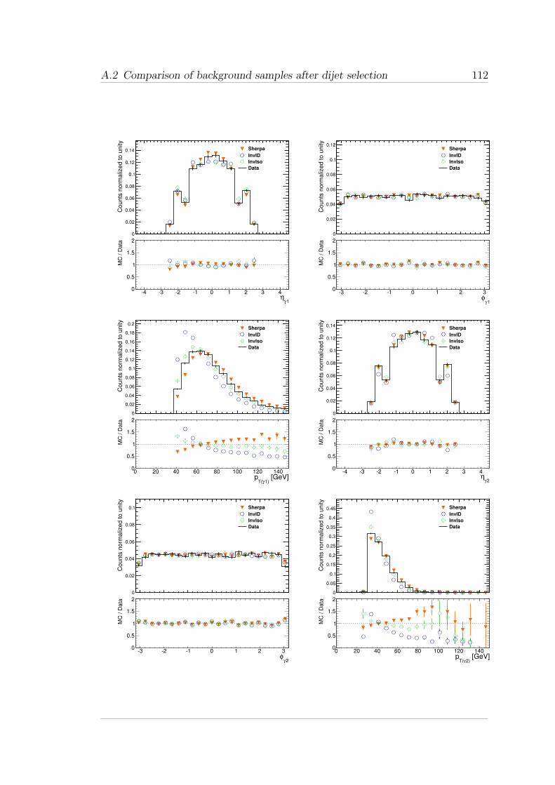
A.2 Comparison of background samples after dijet selection 112
Co
un
ts n
orm
aliz
ed
to
un
ity
0
0.02
0.04
0.06
0.08
0.1
0.12
0.14 Sherpa
InvID
InvIso
Data
1γη
-4 -3 -2 -1 0 1 2 3 4
MC
/ D
ata
0
0.5
1
1.5
2
Co
un
ts n
orm
aliz
ed
to
un
ity
0
0.02
0.04
0.06
0.08
0.1
0.12Sherpa
InvID
InvIso
Data
1γφ
-3 -2 -1 0 1 2 3
MC
/ D
ata
0
0.5
1
1.5
2
Co
un
ts n
orm
aliz
ed
to
un
ity
0
0.02
0.04
0.06
0.08
0.1
0.12
0.14
0.16
0.18
0.2Sherpa
InvID
InvIso
Data
[GeV]1)γT(
p0 20 40 60 80 100 120 140
MC
/ D
ata
0
0.5
1
1.5
2
Co
un
ts n
orm
aliz
ed
to
un
ity
0
0.02
0.04
0.06
0.08
0.1
0.12
0.14Sherpa
InvID
InvIso
Data
2γη
-4 -3 -2 -1 0 1 2 3 4
MC
/ D
ata
0
0.5
1
1.5
2
Co
un
ts n
orm
aliz
ed
to
un
ity
0
0.02
0.04
0.06
0.08
0.1 Sherpa
InvID
InvIso
Data
2γφ
-3 -2 -1 0 1 2 3
MC
/ D
ata
0
0.5
1
1.5
2
Co
un
ts n
orm
aliz
ed
to
un
ity
0
0.05
0.1
0.15
0.2
0.25
0.3
0.35
0.4
0.45 Sherpa
InvID
InvIso
Data
[GeV]2)γT(
p0 20 40 60 80 100 120 140
MC
/ D
ata
0
0.5
1
1.5
2
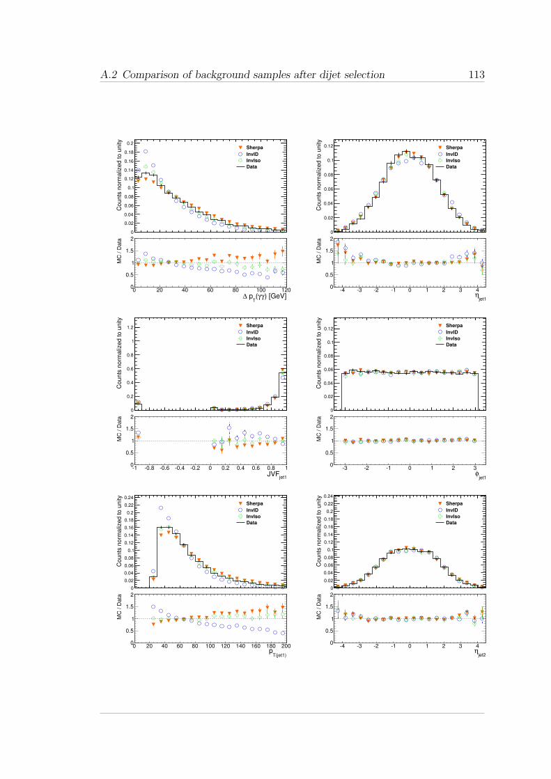
A.2 Comparison of background samples after dijet selection 113
Co
un
ts n
orm
aliz
ed
to
un
ity
0
0.02
0.04
0.06
0.08
0.1
0.12
0.14
0.16
0.18
0.2Sherpa
InvID
InvIso
Data
) [GeV]γγ(T
p∆0 20 40 60 80 100 120
MC
/ D
ata
0
0.5
1
1.5
2
Co
un
ts n
orm
aliz
ed
to
un
ity
0
0.02
0.04
0.06
0.08
0.1
0.12 Sherpa
InvID
InvIso
Data
jet1η
-4 -3 -2 -1 0 1 2 3 4
MC
/ D
ata
0
0.5
1
1.5
2
Co
un
ts n
orm
aliz
ed
to
un
ity
0
0.2
0.4
0.6
0.8
1
1.2 Sherpa
InvID
InvIso
Data
jet1JVF
-1 -0.8 -0.6 -0.4 -0.2 0 0.2 0.4 0.6 0.8 1
MC
/ D
ata
0
0.5
1
1.5
2
Co
un
ts n
orm
aliz
ed
to
un
ity
0
0.02
0.04
0.06
0.08
0.1
0.12Sherpa
InvID
InvIso
Data
jet1φ
-3 -2 -1 0 1 2 3
MC
/ D
ata
0
0.5
1
1.5
2
Co
un
ts n
orm
aliz
ed
to
un
ity
0
0.02
0.04
0.06
0.08
0.1
0.12
0.14
0.16
0.18
0.2
0.22
0.24
Sherpa
InvID
InvIso
Data
T(jet1)p
0 20 40 60 80 100 120 140 160 180 200
MC
/ D
ata
0
0.5
1
1.5
2
Co
un
ts n
orm
aliz
ed
to
un
ity
0
0.02
0.04
0.06
0.08
0.1
0.12
0.14
0.16
0.18
0.2
0.22
0.24
Sherpa
InvID
InvIso
Data
jet2η
-4 -3 -2 -1 0 1 2 3 4
MC
/ D
ata
0
0.5
1
1.5
2
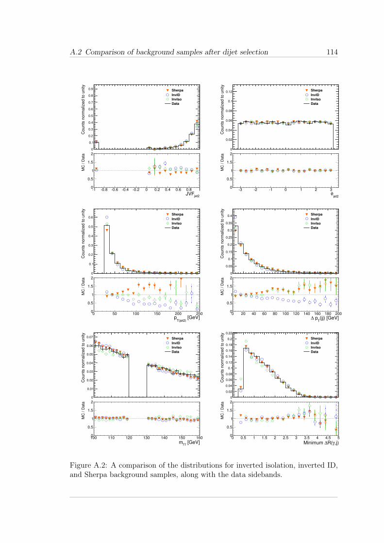
A.2 Comparison of background samples after dijet selection 114
Co
un
ts n
orm
aliz
ed
to
un
ity
0
0.1
0.2
0.3
0.4
0.5
0.6
0.7
0.8
0.9 Sherpa
InvID
InvIso
Data
jet2JVF
-1 -0.8 -0.6 -0.4 -0.2 0 0.2 0.4 0.6 0.8 1
MC
/ D
ata
0
0.5
1
1.5
2
Co
un
ts n
orm
aliz
ed
to
un
ity
0
0.02
0.04
0.06
0.08
0.1
0.12 Sherpa
InvID
InvIso
Data
jet2φ
-3 -2 -1 0 1 2 3
MC
/ D
ata
0
0.5
1
1.5
2
Co
un
ts n
orm
aliz
ed
to
un
ity
0
0.1
0.2
0.3
0.4
0.5
0.6Sherpa
InvID
InvIso
Data
[GeV]T(jet2)
p0 50 100 150 200 250
MC
/ D
ata
0
0.5
1
1.5
2
Co
un
ts n
orm
aliz
ed
to
un
ity
0
0.05
0.1
0.15
0.2
0.25
0.3
0.35
0.4 Sherpa
InvID
InvIso
Data
(jj) [GeV]T
p∆0 20 40 60 80 100 120 140 160 180 200
MC
/ D
ata
0
0.5
1
1.5
2
Co
un
ts n
orm
aliz
ed
to
un
ity
0
0.01
0.02
0.03
0.04
0.05
0.06
0.07 Sherpa
InvID
InvIso
Data
[GeV]γγm100 110 120 130 140 150 160
MC
/ D
ata
0
0.5
1
1.5
2
Co
un
ts n
orm
aliz
ed
to
un
ity
0
0.02
0.04
0.06
0.08
0.1
0.12
0.14
0.16
0.18
0.2
0.22
Sherpa
InvID
InvIso
Data
,j)γR(∆Minimum 0 0.5 1 1.5 2 2.5 3 3.5 4 4.5 5
MC
/ D
ata
0
0.5
1
1.5
2
Figure A.2: A comparison of the distributions for inverted isolation, inverted ID,and Sherpa background samples, along with the data sidebands.
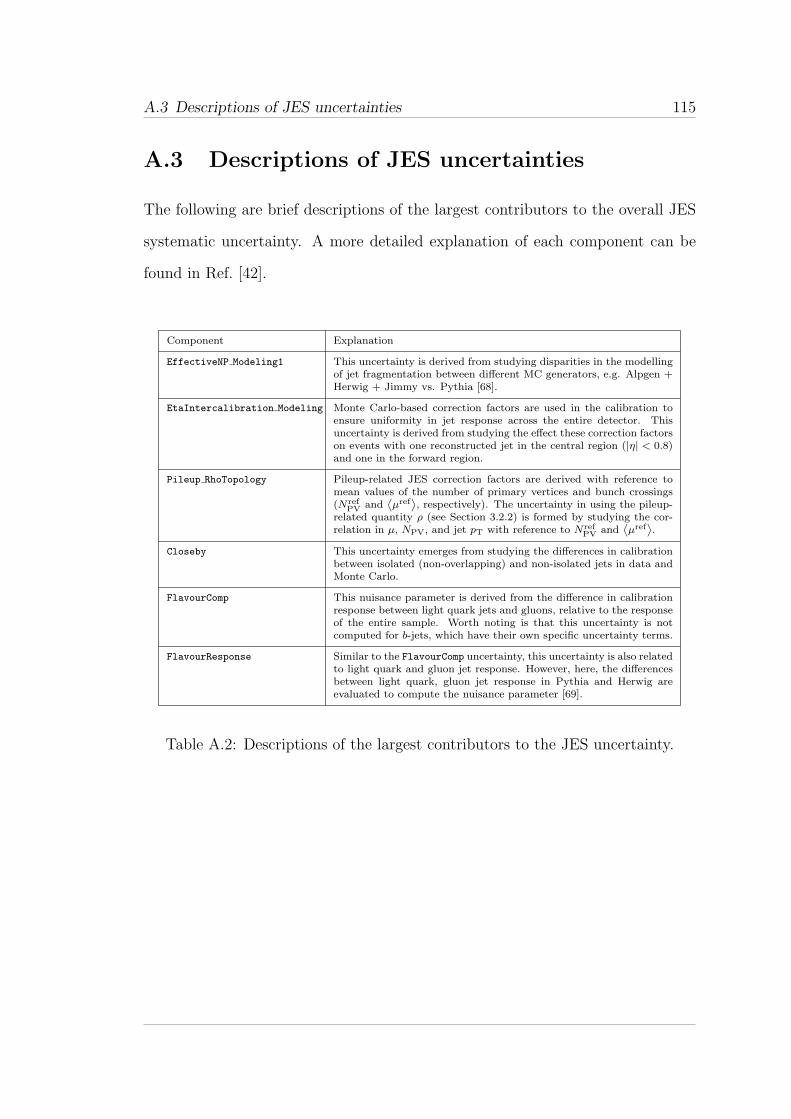
A.3 Descriptions of JES uncertainties 115
A.3 Descriptions of JES uncertainties
The following are brief descriptions of the largest contributors to the overall JES
systematic uncertainty. A more detailed explanation of each component can be
found in Ref. [42].
Component Explanation
EffectiveNP Modeling1 This uncertainty is derived from studying disparities in the modellingof jet fragmentation between different MC generators, e.g. Alpgen +Herwig + Jimmy vs. Pythia [68].
EtaIntercalibration Modeling Monte Carlo-based correction factors are used in the calibration toensure uniformity in jet response across the entire detector. Thisuncertainty is derived from studying the effect these correction factorson events with one reconstructed jet in the central region (|η| < 0.8)and one in the forward region.
Pileup RhoTopology Pileup-related JES correction factors are derived with reference tomean values of the number of primary vertices and bunch crossings(Nref
PV and⟨
µref⟩
, respectively). The uncertainty in using the pileup-related quantity ρ (see Section 3.2.2) is formed by studying the cor-relation in µ, NPV, and jet pT with reference to Nref
PV and⟨
µref⟩
.
Closeby This uncertainty emerges from studying the differences in calibrationbetween isolated (non-overlapping) and non-isolated jets in data andMonte Carlo.
FlavourComp This nuisance parameter is derived from the difference in calibrationresponse between light quark jets and gluons, relative to the responseof the entire sample. Worth noting is that this uncertainty is notcomputed for b-jets, which have their own specific uncertainty terms.
FlavourResponse Similar to the FlavourComp uncertainty, this uncertainty is also relatedto light quark and gluon jet response. However, here, the differencesbetween light quark, gluon jet response in Pythia and Herwig areevaluated to compute the nuisance parameter [69].
Table A.2: Descriptions of the largest contributors to the JES uncertainty.
Appendix B
Personal contributions to the
ATLAS collaboration
Several collaborators worked together to develop the VBF H → γγ multivariate
analysis, which superseded the former cut-based categorization, thereby becoming
an integral part of the ATLAS H → γγ analysis. Furthermore, many others
were involved in performing the final statistical analysis. Therefore, this section
details my most significant contributions to the analysis, and the relevant chapters
in which the work is found, along with my contributions to the larger ATLAS
collaboration.
1. Development and testing of H → γγ analysis software for the Canadian
VBF H → γγ group
⊲ Relevant chapter: Chapter 3
⊲ Summary of contribution: In preparation for the new VBF analysis,
I assumed the lead developer role for the H → γγ analysis software that
had previously been developed and maintained by Canadian VBF H →γγ group members D. Gillberg and F. Bernlochner. This task involved
continually updating the event selection to meet the standards laid
out by the lead analyzers, incorporating new tools and event weights,
116
117
restructuring and optimizing C++ code, and testing the code to ensure
agreement with other analyzers. I also contributed a significant portion
of the code used by the Canadian group to perform the final BDT
analysis.
2. Production of data and Monte Carlo samples for the Canadian VBF H →γγ group
⊲ Relevant chapters: Chapter 3, Chapter 6
⊲ Summary of contribution: Once the H → γγ analysis software was
stable, it was necessary to produce skims of both ATLAS data, and
the signal, background Monte Carlo samples used in the multivariate
analysis. I was wholly responsible for producing and validating these
skims for the Canadian VBFH → γγ group, as well as putting together
a centralized archive for their storage and access. I also produced skims
of the differently-tuned ggF samples for Section 6.1.4.
3. Background model studies for Monte Carlo and data-driven samples
⊲ Relevant chapters: Chapter 4, Chapter 5
⊲ Summary of contribution: Much of the original ideas and deriva-
tion of the “rough” BDT analysis came from the Canadian VBF H →γγ group. I contributed to discussions within the MVA group on possi-
ble background models, and performed studies comparing the different
models in Table 4.1 with regard to their accuracy in modelling the
sideband data, the results of which are shown in Figure A.2. Though
proposed by other members of the MVA group, I also contributed a
study of the accuracy of the mixed background model discussed in Sec-
tion 5.1.
4. Derivation of the benchmark list of BDT classifiers
⊲ Relevant chapter: Chapter 4
⊲ Summary of contribution: The input variable selection and opti-
mization processes detailed in Sections 4.4.2 and 4.4.1 were devised by
118
myself and other Canadian group members. I procured the initial list
of variables, performed the initial training, and ranked variables based
on separation and importance, with the subsequent BDTs trained and
generated by F. Bernlochner. I then performed the significance calcu-
lations, rankings, etc. and generated the resultant benchmark variable
list.
5. Derivation of the optimal BDT configuration
⊲ Relevant chapter: Chapter 5
⊲ Summary of contribution: The BDT configuration optimization
process was also developed by myself and F. Bernlochner, and subse-
quently adopted by the MVA group. As in the benchmark variable list
derivation, I devised a series of parameters to test, and developed the
final analysis and ranking, while F. Bernlochner performed the BDT
training.
6. Calculation of JES and JER systematic uncertainties
⊲ Relevant chapters: Chapter 6, Chapter 7
⊲ Summary of contribution: I was responsible for the evaluation of
both the JES and JER systematic uncertainties, as detailed in Chap-
ter 6, which are large contributors to the detector-related uncertainties
in the VBF H → γγ analysis. I was also responsible for presenting
these results to the larger H → γγ group in a format usable for the
statistical analysis of Chapter 7.
7. Liquid argon data quality & inspection shift work
⊲ Summary of contribution: During my shift work, I was responsible
for the offline evaluation of the quality of recently recorded calorime-
ter data. Tasks include scanning data for high voltage trips, noise
bursts, and instances of non-trivial data rejection during data acqui-
sition. Noisy calorimeter cells were flagged for vetoing, and lists of
defects in luminosity blocks were uploaded to a database for further
event cleaning. Presentations were also prepared for daily and weekly
119
meetings which summarized the status of each run inspected, and re-
layed any systematic problems with calorimeter behaviour. For this
shift work, I received Class 3 OTP credit for Carleton University.
8. Authorship qualification task in electron-photon group
⊲ Summary of contribution: My authorship qualification task in-
volved the revival and development of a method to combine electron
track and cluster four momentum measurements into a single, optimal
four momentum (an E−p combination). Initial studies were performed
to determine the optimal circumstances for combination, in terms of
observable quantities that were correlated with truth-level information,
and the quality of the track and cluster reconstruction, such as the
approximate amount of bremsstrahlung losses in the Inner Detector.
Validation was then performed on a variety of data and Monte Carlo
samples: J/ψ and Z → ee decays; single electron samples; andH → ZZ
→ 4l decays. In addition to developing the method for the combina-
tion, I rewrote existing E − p combination software to implement the
new method, optimize the C++ code, and enhance code modularity
and readability. For this task, I received my authorship qualification.
Furthermore, a public conference note on the tool’s development is in
progress, and will make up a component of a future paper on electron
calibration by the ATLAS electron-photon group.
Recommended