Copyright InterAC 1
10 impasse Borde-basse Z. A. La Violette SARL au capital de 50 000 Euros 31240 L'Union France RCS Toulouse B 389 259 706 TEL 33 (0)5 61 09 47 45 SIRET 389 259 706 00031 FAX 33 (0)5 61 74 62 22 VAT FR10 389 259 706 E-mail: [email protected] www.interac.fr APE 7490B
SEA-TEST version info
Summary
PRESENTATION .................................................................................................................................................. 2
WHY MEASURING DLF AND CLF? ................................................................................................................ 3
SEPARATING INTERNAL AND COUPLING LOSSES ................................................................................................... 3 ANALYZING SUBSYSTEM POLYMORPHISM............................................................................................................ 4
SEA MODELS FOR NON-HOMOGENOUS STRUCTURES ......................................................................... 4
ACOUSTIC AND STRUCTURAL COUPLING ................................................................................................ 6
EXPORTING ESEA MODEL TO ANALYTICAL SEA SOFTWARE ............................................................ 7
REVIEW OF SEA-TEST EVOLUTION ............................................................................................................ 7
VERSION 1.0 (OCTOBER 2006) ........................................................................................................................ 7
VERSION 2007-03 (AUGUST 2007) ................................................................................................................... 7
ADDING FUNCTIONALITIES .................................................................................................................................. 7 BUGS FIXED AND ENHANCEMENTS ...................................................................................................................... 7
VERSION 2007-04 (NOVEMBER 2007) ............................................................................................................ 8
ADDING FUNCTIONALITIES .................................................................................................................................. 8 BUGS FIXED AND ENHANCEMENTS ...................................................................................................................... 8
VERSION 2008-1 (APRIL 2008) ......................................................................................................................... 8
VERSION 2008-1.1 (JULY 2008) ......................................................................................................................... 8
VERSION 2008-2 (OCTOBER 2008) .................................................................................................................. 8
VERSION 2009 (OCTOBER 2009) ..................................................................................................................... 8
VERSION 2011 (OCTOBER 2011)...................................................................................................................... 8
VERSION 2012 (OCTOBER 2012) ..................................................................................................................... 9
VERSION 2013 (DECEMBER 2013) .................................................................................................................. 9
VERSION 2013.0.2 (JULY 2014) ......................................................................................................................... 9
VERSION 2016 (FEBRUARY 2016) MAJOR RELEASE ................................................................................ 9

Copyright InterAC 2
Presentation
InterAC Experimental SEA (ESEA) Software: SEA-XP/SEA-TEST has been evolving
continuously for the last past ten years to fit with the complexity of industrial design. This
software is mainly an evolution of early routines developed from 1991 by Dr. G. Borello to
build SEA model of industrial engines. With the help of SEP (Société d’Etudes et de Propulsion)
that has been designing the cryogenic rocket engine of Ariane 5, Vulcain, these routines have
been turned progressively into a full operational software combining both acquisition and post-
processing for a maximum of performance.
Starting from decomposition into subsystems of the system to be analyzed, SEA-XP/SEA-
TEST is solving the active power balanced equations by measuring transfer acceleration and
input power. More precisely the measured quantities are FRF’s (Frequency Response
Functions) and input conductances as all accelerations are stored in FRF format and only the
real part of the normalized input power/force² is used in the power equilibrium.
Here below, one of the first SEA-XP/SEA-TEST application where the experimental power
balanced equations have been solved to build Vulcain hybrid SEA model. The analytical
formulations where provided by the Dr. Borello’s SEA software EARTHS, specifically
designed to model the Vulcain and completed and validated by import of ESEA parameters.
Figure 1 : The SEA Vulcain model built in 91 with the help of original SEA-XP/SEA-TEST routines and
related
.
COLSEBV
TPHTPO
VCH
D
GG
LE
O
LCH1
LCH2
LTH
LTO
LGH
LCO-TPOLGOVCO
2
3
4 5
67
89
1011
13
14
15
16
12
VGO
LE
H
VGH
1
DIVERGENT
Copyright InterAC 3
Why measuring DLF and CLF?
Separating internal and coupling losses
In most cases, the Damping Loss Factors (DLF) of industrial structures cannot be computed
theoretically. They are also depending on the assembly and thus cannot be determined from
individual tests.
More of it, simple tests such as decay rate measurement cannot provide good enough estimates
of subsystem DLF. In fact the DLF of a subsystem in a coupled model is related to the power
loss that is intrinsically dissipated within this subsystem and which is not related directly to the
decay rate of its impulse response. The decay rate is only proportional to the total loss related
to a given subsystem i.e. sum of the intrinsic power loss within this subsystem and to the power
dissipated in the coupling (that escapes to the other coupled subsystems). Thus the decay rate
includes information about both intrinsic power loss and coupling loss.
The power losses into the coupling between subsystems are characterized by the related
Coupling Loss Factors (CLF).
The CLF level is depending upon the mechanical connection between subsystems.
To compute these coefficients in the high frequency domain, analytical SEA heavily relies on
simplified hypothesis: ideal diffusion of energy, plane wave assumption, simple line or point
connected junctions of homogeneous simple plates or shells. On real structures, junctions are
far ahead in term of complexity.
ESEA, by measuring all transfer velocities and input conductances from a set of simple impact
or acoustic tests, is able to identify both intrinsic DLF and the CLF between any subsystems.
The subsystems must exhibit local modal behavior in the frequency range of interest for the
inverse problem identification to be successful and is de facto a “high frequency measurement”
technique.
SEA model of complex industrial machines can thus be built with the help of this technology.
Using the SEA-XP/SEA-TEST estimates of CLF, it is possible to tune simple adequate
theoretical models of junctions in order to perform parametric changes and noise reduction
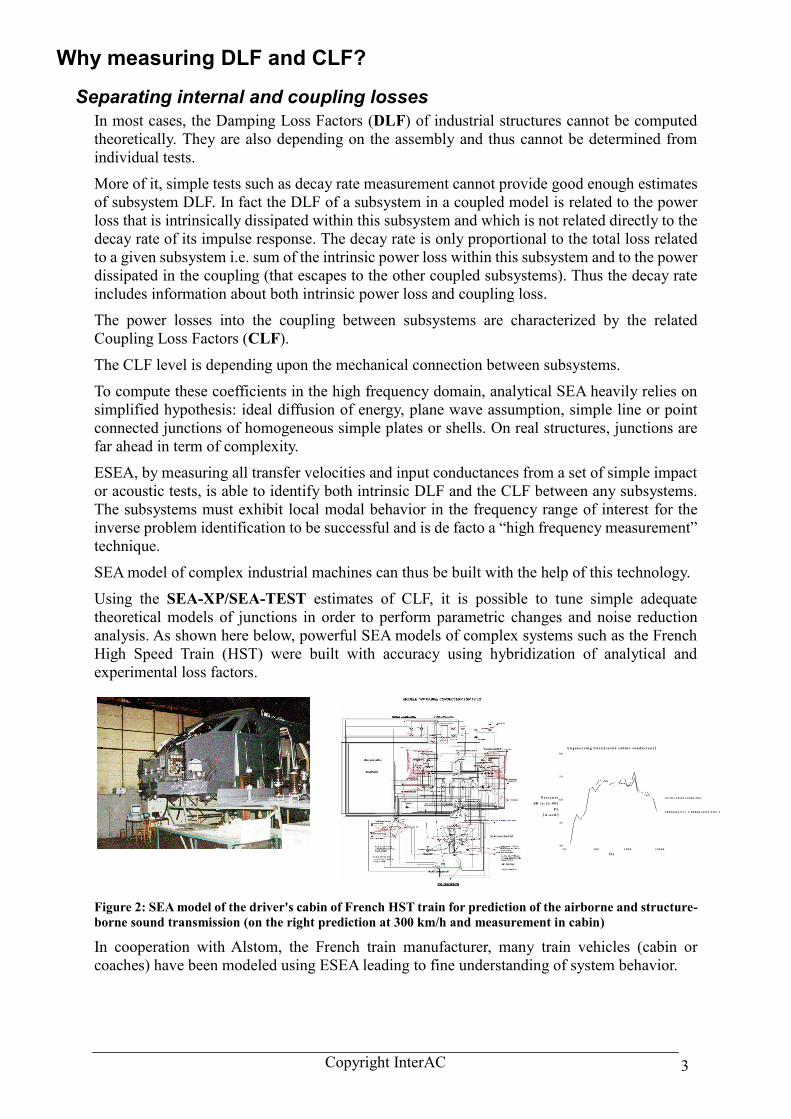
analysis. As shown here below, powerful SEA models of complex systems such as the French
High Speed Train (HST) were built with accuracy using hybridization of analytical and
experimental loss factors.
Figure 2: SEA model of the driver's cabin of French HST train for prediction of the airborne and structure-
borne sound transmission (on the right prediction at 300 km/h and measurement in cabin)
In cooperation with Alstom, the French train manufacturer, many train vehicles (cabin or
coaches) have been modeled using ESEA leading to fine understanding of system behavior.
En g i n e e r i n g U n i ts [ca vi té ca bi n e co n du cte u r]
1 0 1 0 0 1 0 0 0 1 0 0 0 0
H z
3 0
4 5
6 0
7 5
9 0
P re s s u re
dB re :2 e -0 0 5
P a
[A -w td.]
c a vi té c a b i n e c o n d u c te u r
3 0 0 k m h A T 1 7 _ C h 0 B l k 1 .PA 3 .T X T -1

Copyright InterAC 4
Analyzing subsystem polymorphism
ESEA helps in understanding the polymorphism of subsystems (evolution of dynamical
behaviour vs. frequency).
When applying experimental and analytical SEA to car modeling, it rapidly comes to an end
that the frequency range of interest (100-2000 Hz) was very difficult to be successfully covered
using only analytical description of subsystems.
Looking on the rear pillar shape of a car roof (Figure 3), it can be clearly seen that it is not easy
to confine its SEA description in term of simple analytical beam or plate.
From ESEA, we learn about this subsystem by measuring both input conductance and CLF. It
appears that this subsystem can be seen as SEA beam at low frequency and as SEA plate at
higher frequency. The transition frequency domain just lies in the 800-1000 Hz.
Figure 3: Analyzing subsystem polymorphism of car subsystem with ESEA
Most of the SEA subsystems of a car exhibit this dramatic change of dynamical behavior in this
mid-frequency region, leading to difficulty in applying a “static” analytical description for each
of them as required in commercial analytical SEA software.
ESEA was thus used to find “equivalent” SEA analytical representation that could fit to the
observed dynamical behavior.
SEA models for non-homogenous structures ESEA is very useful to understand how non-homogeneous subsystems behave.
Non-homogeneous subsystems are characterized by some non constant parameters that can vary
within the subsystem domain: non constant thickness, radius of curvature, material…
A car is typically made of many non-homogeneous subsystems.
Classical analytical SEA is ideal for homogeneous subsystems but how to derive an analytical
representation of a shell with a non constant radius of curvature as an example?
ESEA is using a multi-transducer approach to solve elegantly this problem.
In place of describing the subsystem by a single power balanced equation, referenced to a
particular excitation (or to a particular transducer in reciprocal measurement), it uses as many
power balanced equations as required with several reference excitation spread at various
locations of the subsystem. Using more equations than unknowns in the solve process, it is
possible to find a best-fitted experimental set of SEA parameters to characterized this non-
homogeneous subsystem from the pseudo-inverse of the energy matrix (with a Singular Value
Decomposition or SVD solver).
Non-homogeneous subsystems are also characterized by high variability of velocity when
scanning the subsystem domain. All estimates of measured energy and power are thus affected
by some variance depending upon subsystem complexity.
beam modesPlat e modes
Unit force
Example : Cent ral Side f rame
Experimental/theoretical Input mobility in the central side frame
10 100 1000 10000
Hz
1e-08
1e-07
1e-06
1e-05
0.0001
0.001
0.01
0.1
PowerWatt
SEA Mobility in Plate
ASEI Test mobility
SEA Mobility in Beam
beam behaviour
t heoret ical 1mm plat e behaviour

Copyright InterAC 5
When simply inverting the transferred energy matrix once, some SEA parameters can be
negative on output and not really representative of the real statistical behavior of the subsystem.
A Monte-Carlo procedure has been introduced in the solve process to overcome SEA parameter
dispersion:
- when recording the data, variance is computed for all inputs;
- when solving, the input data set is perturbed, following related variance of each of the input
and the output set of SEA parameters is averaged with previous results obtained for another
perturbation of the input data set;
- the solve process can be run in loops several thousand of time in order to derive statistic
and variance on output; some solution sets that are obviously non physical can thus be
rejected from the averaged solution (i.e. SEA sets that incorporates too many negative CLF
of DLF values);
- the SEA loss matrix final solution can be characterized by a performance index, providing
confidence in the result.
Figure 4: ESEA data flow
The velocity to energy conversion is performed through an “equivalent mass” term which is
determined experimentally from the analysis of the decay rate of impulse responses of recorded
FRF. This mass term is generally frequency-dependant as we deal with complex subsystems.
The mass is nearly independent from frequency only for homogeneous simple systems. The use
of equivalent mass in SEA is greatly improving dynamical behavior understanding and its
computation does not require any additional measurement as it is fully automated in SEA-
XP/SEA-TEST.
Matrix of transfer velocities
Vector of input mobilities
Recording Narrow
band Complex FRF
of acceleration
transfers
Measurement
on a grid of
nodes on the
physical
object Integration over
Freq. band
Averaging over subsystem
domain and variance estimate
SEA model
performance
Step 1
Step 2
Step 3
Step 4
Step 5
Targeted
Freq. Band
SEA direct solver or export
to external SEA software
Monte Carlo
process Inverse SEA problem
variance
Copyright InterAC 6
Acoustic and structural coupling Most of the uncertainty in SEA models is contained in structural subsystems and SEA-
XP/SEA-TEST was designed from the beginning to focus on structure borne sound
transmission. Nevertheless, a full acoustic-to-structure analysis has been included in the
software in the mid-nineties.
Within SEA-XP/SEA-TEST, the only difference between acoustic SEA subsystems and
structural subsystems is the type of recorded data. Generally, pressure measurement is used for
acoustics and acceleration for structures. In SEA-XP/SEA-TEST, the data type for acoustics
is a FRF computed as “pressure signal /reference signal”. When computing the mean squared
transfer velocity from the FRF, the software automatically converts all acoustic FRF into
velocity spectra, using an impedance term (the acoustic impedance) that is defined for each
record.
After averaging into squared velocity, there is no more difference between cavity and structures
in the data set.
Various problems can be addressed by ESEA, from pure cavity coupling to full vibroacoustic
analysis.
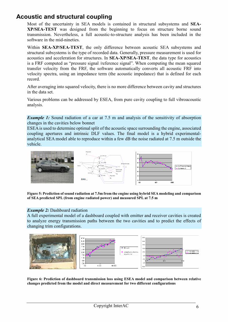
Example 1: Sound radiation of a car at 7.5 m and analysis of the sensitivity of absorption
changes in the cavities below bonnet
ESEA is used to determine optimal split of the acoustic space surrounding the engine, associated
coupling apertures and intrinsic DLF values. The final model is a hybrid experimental-
analytical SEA model able to reproduce within a few dB the noise radiated at 7.5 m outside the
vehicle.
Figure 5: Prediction of sound radiation at 7.5m from the engine using hybrid SEA modeling and comparison
of SEA predicted SPL (from engine radiated power) and measured SPL at 7.5 m
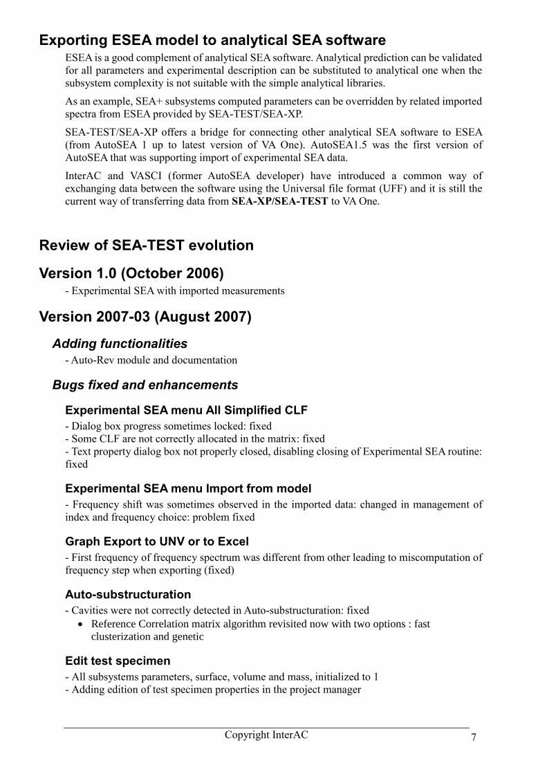
Example 2: Dashboard radiation
A full experimental model of a dashboard coupled with emitter and receiver cavities is created
to analyze energy transmission paths between the two cavities and to predict the effects of
changing trim configurations.
Figure 6: Prediction of dashboard transmission loss using ESEA model and comparison between relative
changes predicted from the model and direct measurement for two different configurations
config1.nwk 11:16:20 28/09/98
Vol 1 AVH 3SVol 2 DH
Vol 3 ARH pinj
Vol 4 GH
Vol 5 AVB
Vol 6 DB
Vol 7 ARBB
Vol 8 GB
Ext D 3 pinj
Ext G Bas de caisse
AR and AV side
Pinj Vol 3
Pinj Vol 2
Pinj Vol 6
Copyright InterAC 7
Exporting ESEA model to analytical SEA software ESEA is a good complement of analytical SEA software. Analytical prediction can be validated
for all parameters and experimental description can be substituted to analytical one when the
subsystem complexity is not suitable with the simple analytical libraries.
As an example, SEA+ subsystems computed parameters can be overridden by related imported
spectra from ESEA provided by SEA-TEST/SEA-XP.
SEA-TEST/SEA-XP offers a bridge for connecting other analytical SEA software to ESEA
(from AutoSEA 1 up to latest version of VA One). AutoSEA1.5 was the first version of
AutoSEA that was supporting import of experimental SEA data.
InterAC and VASCI (former AutoSEA developer) have introduced a common way of
exchanging data between the software using the Universal file format (UFF) and it is still the
current way of transferring data from SEA-XP/SEA-TEST to VA One.
Review of SEA-TEST evolution
Version 1.0 (October 2006) - Experimental SEA with imported measurements
Version 2007-03 (August 2007)
Adding functionalities
- Auto-Rev module and documentation
Bugs fixed and enhancements
Experimental SEA menu All Simplified CLF
- Dialog box progress sometimes locked: fixed
- Some CLF are not correctly allocated in the matrix: fixed
- Text property dialog box not properly closed, disabling closing of Experimental SEA routine:
fixed
Experimental SEA menu Import from model
- Frequency shift was sometimes observed in the imported data: changed in management of
index and frequency choice: problem fixed
Graph Export to UNV or to Excel
- First frequency of frequency spectrum was different from other leading to miscomputation of
frequency step when exporting (fixed)
Auto-substructuration
- Cavities were not correctly detected in Auto-substructuration: fixed
Reference Correlation matrix algorithm revisited now with two options : fast
clusterization and genetic
Edit test specimen
- All subsystems parameters, surface, volume and mass, initialized to 1
- Adding edition of test specimen properties in the project manager

Copyright InterAC 8
Experimental SEA solver
- Improvement of Loss matrix optimizer: performance index now computed by same routine,
adding local global performance index and extra menu
- Import from model: now loss factors from subsystems with same name can be averaged
between imported and targeted models
- New subsystem edition pane (parallel editing)
- Possible manual import of 1/3 octave spectrum in any item of the experimental SEA model
Version 2007-04 (November 2007)
Adding functionalities
- V_R protocol for non homogeneous system and theory
- Creating geometry from FE exported data
Bugs fixed and enhancements
- Time reverberation in AutoRev
Version 2008-1 (April 2008) Updating the user’s guide to explain “reduced velocity” solve
Version 2008-1.1 (July 2008) - Change licensing protection from hasp key to license file
- AutoRev reverberation time analysis can be extended to very low frequency (limit 1 Hz)
Version 2008-2 (October 2008) - Automated support is added for P/Q transfers, meaning that the post-processing will be
entirely automatic up to SEA model creation, avoiding mistakes like using ill-defined masses
- Multiple file selection for importing file
- Improved dialog box for “Subsystem Property Characteristic” input
- Possibility to modify manually the sign of a particular FRF of the database using local right-
button menu when selecting a record
- Updating the user-guide to give more practical details on how to measure power, full
documentation on using P/Q transfer functions and overview of the various test protocols
Version 2009 (October 2009) - Import of time measurement in SEA-TEST project component data sheet to compute decay
rate and equivalent mass from time history
- Wav import in AutoRev
Version 2011 (October 2011)
Update to LV runtime engine 2011
- Graphing options have been improved thanks to LV runtime engine 2011.
SEA-Experimental
- In SEA-Experimental, mass calculation of SVD compacted subsystem has been modified
Subsystem mass of compacted subsystems is now equal to the sum of masses of included
subsystems. In previous version, subsystem mass of compacted subsystems was calculated as
mean value of masses of included subsystems
- Upgrade of Export format to VA One (up to version 2010) for correct import of power and
mass

Copyright InterAC 9
- Graphing of reverberation time within Experimental SEA models has been added
Version 2012 (October 2012) - New functionalities added for importing UFF measurements (setting sign and selection).
More options in SEA preferences
- New function for acoustic transfers added: Condensation of p/F transfer on references of a
structural subsystem
- AutoRev: RT cursor algorithm improved to be more stable when using time history
containing audible background noise
Version 2013 (December 2013) Update of all dependencies: LabVIEW 2013, Intel FORTRAN 2013, Net Framework 4
- New function : import Experimental SEA Model from SEA-XP
- New function : "swap CLF"
- Enhancement of function :"Create Geometry"
- Minor bugs fixed (export to dataset 58)
Version 2013.0.2 (July 2014) Update of all dependencies: LabVIEW 2013 SP1f2, Intel FORTRAN 2013 SP1
- Damping Loss Factor computed from time computation changed DLF = 2.2 / (FC*TR)
- Temporary directory read from environment path “TMP_SEA_TEST” if found
- New subsystem compact (patch substructuration)
Bugs fixed
- Characters string exceed the location in the dialog “Show Properties” and in other dialogs
box
- Mass import from text files in properties dialog
- Dialog box Properties cause a crash
Version 2016 (February 2016) major release SEA-TEST 2016 is storing data using the same data engine than SEA+ (SQLite).
Project files are saved with extension *.dbst.
Previous SEA-TEST versions were saved with another file format with extension *.xea.
Prior to open older project files in SEA-TEST 2016, you have to convert them from
XEA to DBST format. SEA-TEST Data_Converter programme is installed with SEA-
TEST 2016.
SEA-TEST interface is entirely re-written to fit new Windows operating system.
Recommended