Scientific Computing with NumPy & SciPy NumPy Installation and Documentation http://numpy.scipy.org/
Not much on the home page—don’t buy the guide, it’s online (see below)
NumPy page at the SciPy site (Better—but not up at the current time)
http://www.scipy.org/NumPy
The fundamental package for scientific computing with Python.
Contains:
a powerful N-dimensional array object
sophisticated functions that accommodate disparities in array dimensions
tools for integrating C/C++ and Fortran code
linear algebra, Fourier transform, and random number capabilities
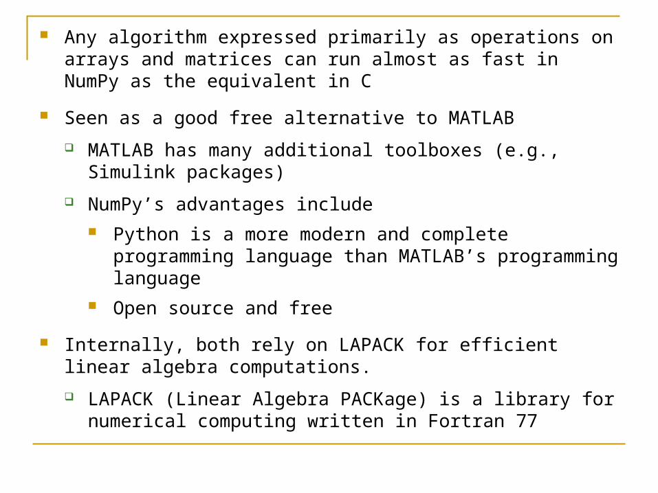
Any algorithm expressed primarily as operations on arrays and matrices can run almost as fast in NumPy as the equivalent in C
Seen as a good free alternative to MATLAB
MATLAB has many additional toolboxes (e.g., Simulink packages)
NumPy’s advantages include Python is a more modern and complete programming
language than MATLAB’s programming language Open source and free
Internally, both rely on LAPACK for efficient linear algebra computations.
LAPACK (Linear Algebra PACKage) is a library for numerical computing written in Fortran 77
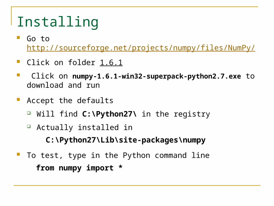
Installing Go to http://sourceforge.net/projects/numpy/files/NumPy/
Click on folder 1.6.1
Click on numpy-1.6.1-win32-superpack-python2.7.exe to download and run
Accept the defaults
Will find C:\Python27\ in the registry
Actually installed in
C:\Python27\Lib\site-packages\numpy
To test, type in the Python command line
from numpy import *
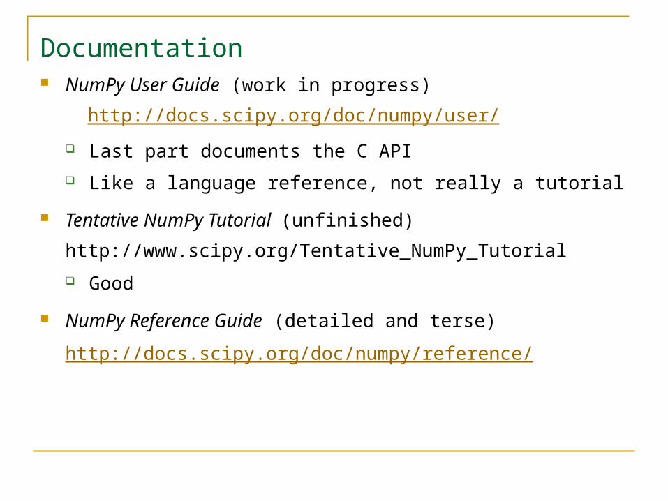
Documentation NumPy User Guide (work in progress)
http://docs.scipy.org/doc/numpy/user/
Last part documents the C API
Like a language reference, not really a tutorial
Tentative NumPy Tutorial (unfinished)
http://www.scipy.org/Tentative_NumPy_Tutorial
Good
NumPy Reference Guide (detailed and terse)
http://docs.scipy.org/doc/numpy/reference/
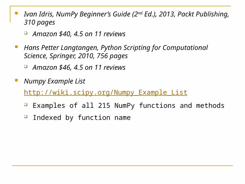
Ivan Idris, NumPy Beginner’s Guide (2nd Ed.), 2013, Packt Publishing, 310 pages
Amazon $40, 4.5 on 11 reviews
Hans Petter Langtangen, Python Scripting for Computational Science, Springer, 2010, 756 pages
Amazon $46, 4.5 on 11 reviews
Numpy Example List
http://wiki.scipy.org/Numpy_Example_List
Examples of all 215 NumPy functions and methods
Indexed by function name
Numpy Example List With Doc
http://wiki.scipy.org/Numpy_Example_List_With_Doc
Auto-generated version of Numpy Example List with added documentation from doc strings and arguments specification for methods and functions
Not all entries have a doc string
Not as regularly updated as Numpy Example List
The SciPy Additional Documentation pagehttp://www.scipy.org/Additional_Documentation?action=show&redirect=Documentation
Has a section for NumPy with numerous links
SciPy Installation and Documentationhttp://www.scipy.org/ An Open Source library of scientific tools for Python
Depends on the NumPy library
Gathers a variety of high level science and engineering modules into one package
Provides modules for statistics optimization numerical integration linear algebra Fourier transforms signal processing image processing genetic algorithms ODE solvers special functions and more
Download Go to http://sourceforge.net/projects/scipy/files/scipy/
Click on folder 0.10.0
Download and execute
scipy-0.10.0-win32-superpack-python2.6.exe
Creates folder
C:\Python27\Lib\site-packages\scipy
To test, try out example under “Basic matrix operations” (the 1st example) in the Tutorial (see below)
Documentation SciPy Tutorial
http://docs.scipy.org/doc/scipy/reference/tutorial/
Travis E. Oliphant, SciPy Tutorial (the “old tutorial”, 42 pp.), 2004.
http://www.tau.ac.il/~kineret/amit/scipy_tutorial/
The example files:
http://www.tau.ac.il/~kineret/amit/scipy_tutorial.tar.gz
Dave Kuhlman, SciPy Course Outline (45 pp.), 2006.
http://www.rexx.com/~dkuhlman/scipy_course_01.html
This is much more than a course outline.
Francisco J. Blanco-Silva, Learning SciPy for Numerical and Scientific Computing, Packt Publishing, 2013, 150 pages
Amazon $26, 4 on 7 reviews
The SciPy Community, SciPy Reference Guide (Release 0.12.0, 1000+ pages), 2013
http://docs.scipy.org/doc/scipy/scipy-ref.pdf
Complete, very much a reference
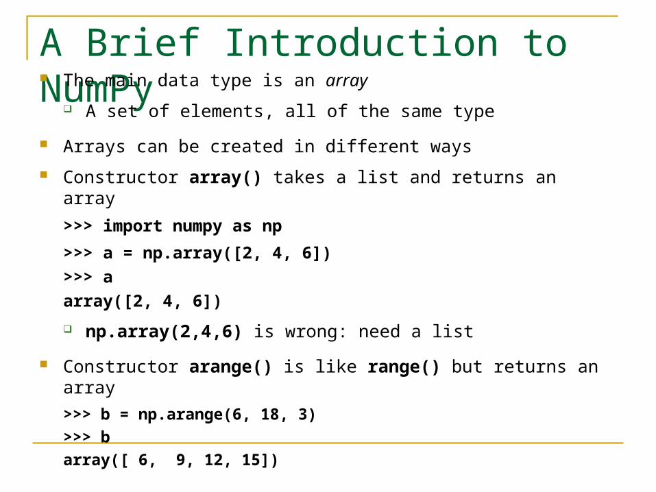
A Brief Introduction to NumPy The main data type is an array
A set of elements, all of the same type
Arrays can be created in different ways
Constructor array() takes a list and returns an array
>>> import numpy as np
>>> a = np.array([2, 4, 6])
>>> a
array([2, 4, 6])
np.array(2,4,6) is wrong: need a list
Constructor arange() is like range() but returns an array
>>> b = np.arange(6, 18, 3)
>>> b
array([ 6, 9, 12, 15])
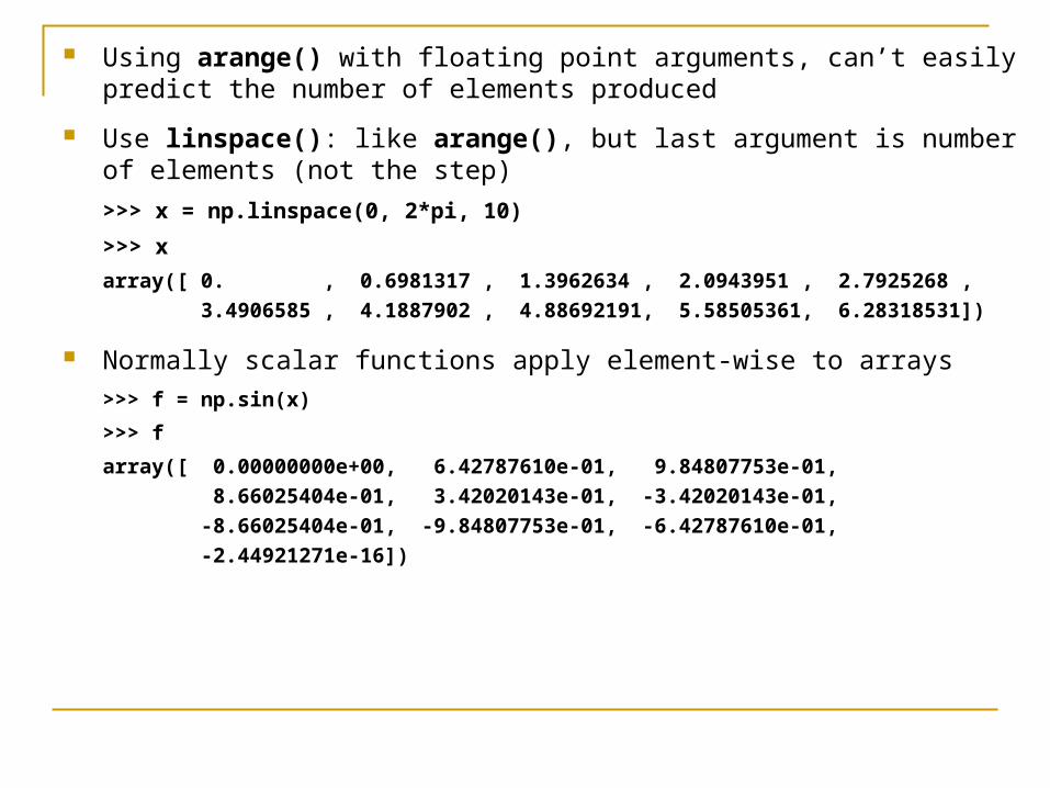
Using arange() with floating point arguments, can’t easily predict the number of elements produced
Use linspace(): like arange(), but last argument is number of elements (not the step)
>>> x = np.linspace(0, 2*pi, 10)
>>> x
array([ 0. , 0.6981317 , 1.3962634 , 2.0943951 , 2.7925268 ,
3.4906585 , 4.1887902 , 4.88692191, 5.58505361, 6.28318531])
Normally scalar functions apply element-wise to arrays
>>> f = np.sin(x)
>>> f
array([ 0.00000000e+00, 6.42787610e-01, 9.84807753e-01,
8.66025404e-01, 3.42020143e-01, -3.42020143e-01,
-8.66025404e-01, -9.84807753e-01, -6.42787610e-01,
-2.44921271e-16])
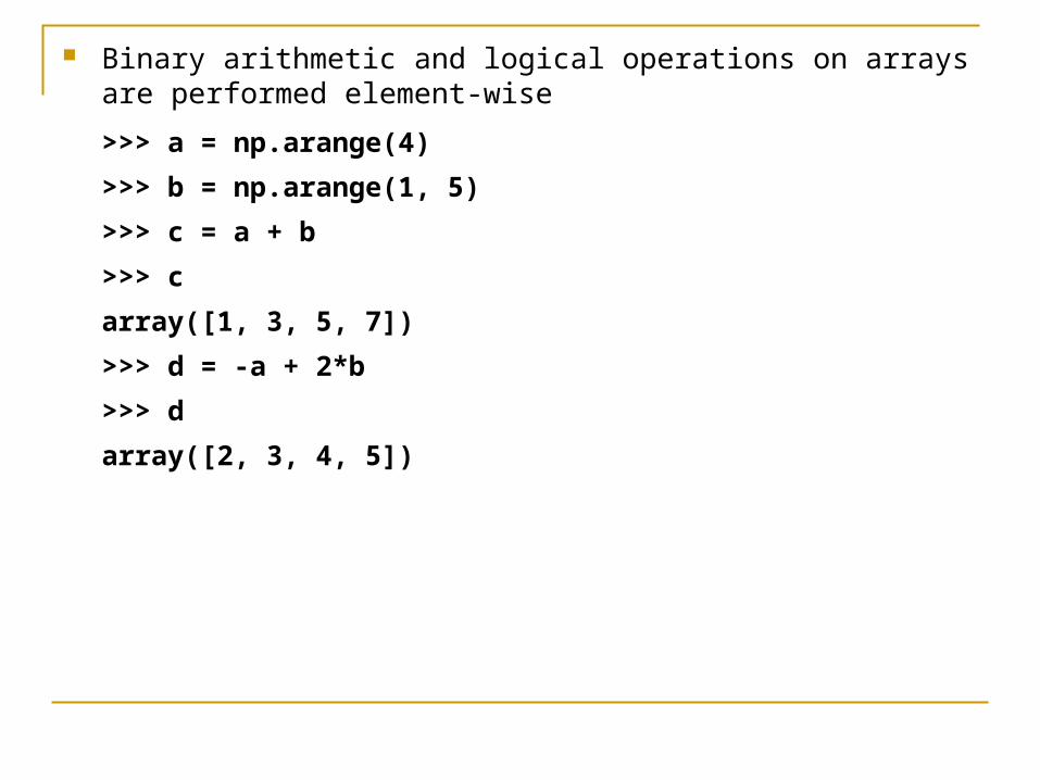
Binary arithmetic and logical operations on arrays are performed element-wise
>>> a = np.arange(4)
>>> b = np.arange(1, 5)
>>> c = a + b
>>> c
array([1, 3, 5, 7])
>>> d = -a + 2*b
>>> d
array([2, 3, 4, 5])
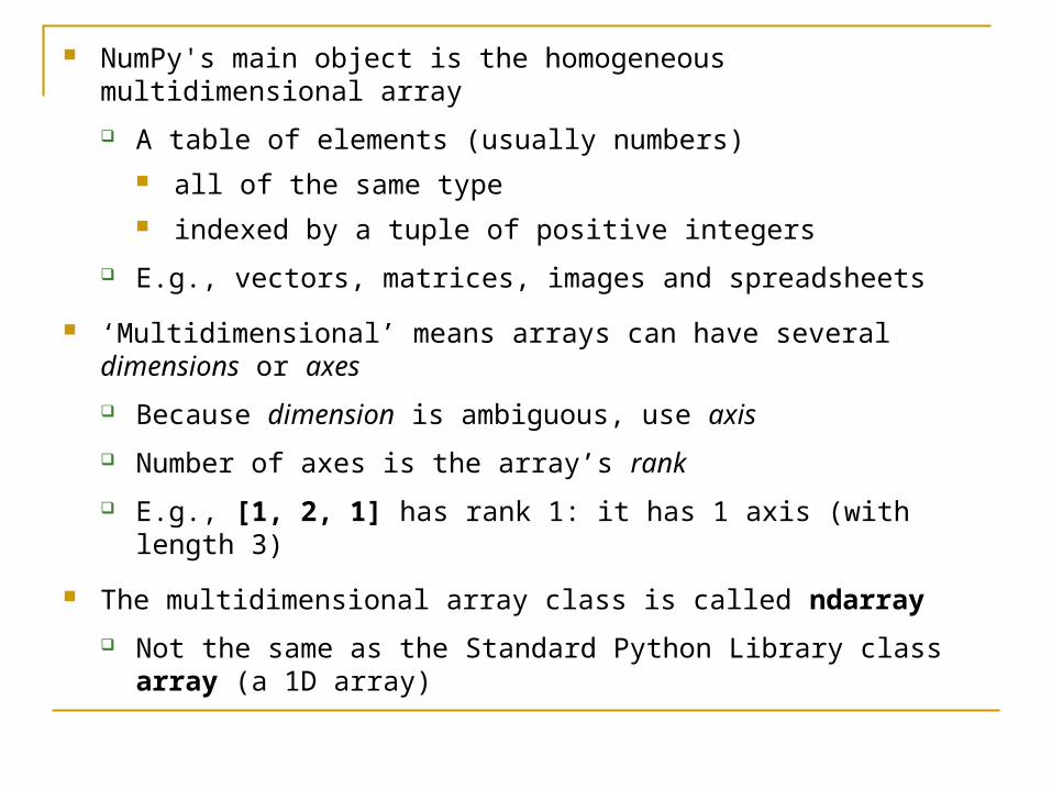
NumPy's main object is the homogeneous multidimensional array
A table of elements (usually numbers) all of the same type indexed by a tuple of positive integers
E.g., vectors, matrices, images and spreadsheets
‘Multidimensional’ means arrays can have several dimensions or axes
Because dimension is ambiguous, use axis
Number of axes is the array’s rank
E.g., [1, 2, 1] has rank 1: it has 1 axis (with length 3)
The multidimensional array class is called ndarray
Not the same as the Standard Python Library class array (a 1D array)
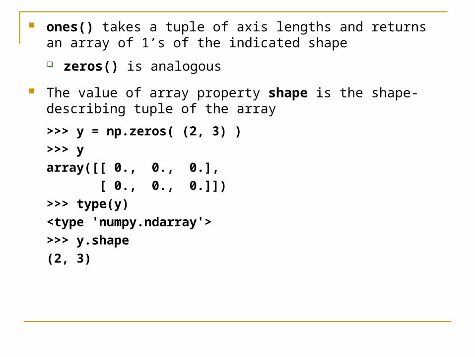
ones() takes a tuple of axis lengths and returns an array of 1’s of the indicated shape
zeros() is analogous
The value of array property shape is the shape-describing tuple of the array
>>> y = np.zeros( (2, 3) )
>>> y
array([[ 0., 0., 0.],
[ 0., 0., 0.]])
>>> type(y)
<type 'numpy.ndarray'>
>>> y.shape
(2, 3)
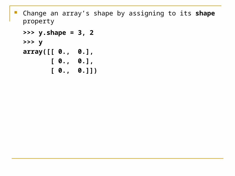
Change an array’s shape by assigning to its shape property
>>> y.shape = 3, 2
>>> y
array([[ 0., 0.],
[ 0., 0.],
[ 0., 0.]])
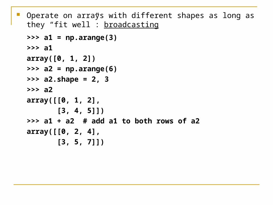
Operate on arrays with different shapes as long as they “fit well”: broadcasting
>>> a1 = np.arange(3)
>>> a1
array([0, 1, 2])
>>> a2 = np.arange(6)
>>> a2.shape = 2, 3
>>> a2
array([[0, 1, 2],
[3, 4, 5]])
>>> a1 + a2 # add a1 to both rows of a2
array([[0, 2, 4],
[3, 5, 7]])
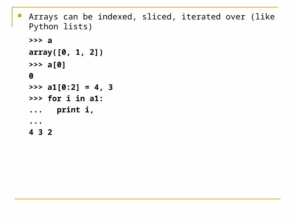
Arrays can be indexed, sliced, iterated over (like Python lists)
>>> a
array([0, 1, 2])
>>> a[0]
0
>>> a1[0:2] = 4, 3
>>> for i in a1:
... print i,
...
4 3 2
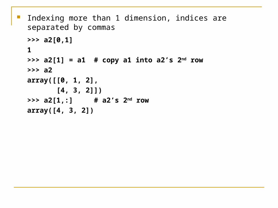
Indexing more than 1 dimension, indices are separated by commas
>>> a2[0,1]
1
>>> a2[1] = a1 # copy a1 into a2’s 2nd row
>>> a2
array([[0, 1, 2],
[4, 3, 2]])
>>> a2[1,:] # a2’s 2nd row
array([4, 3, 2])
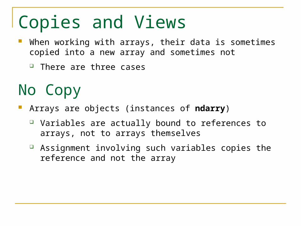
Copies and Views When working with arrays, their data is sometimes copied into a
new array and sometimes not
There are three cases
No Copy Arrays are objects (instances of ndarry)
Variables are actually bound to references to arrays, not to arrays themselves
Assignment involving such variables copies the reference and not the array
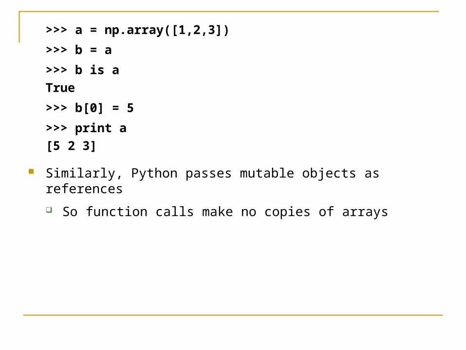
>>> a = np.array([1,2,3])
>>> b = a
>>> b is a
True
>>> b[0] = 5
>>> print a
[5 2 3]
Similarly, Python passes mutable objects as references
So function calls make no copies of arrays
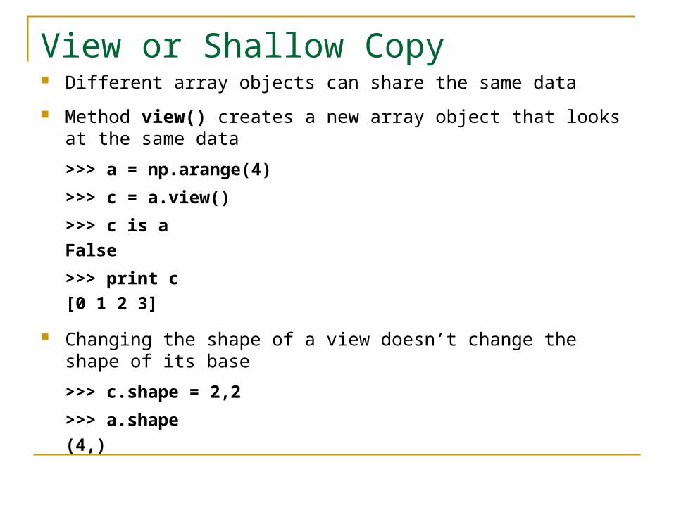
View or Shallow Copy Different array objects can share the same data
Method view() creates a new array object that looks at the same data
>>> a = np.arange(4)
>>> c = a.view()
>>> c is a
False
>>> print c
[0 1 2 3]
Changing the shape of a view doesn’t change the shape of its base
>>> c.shape = 2,2
>>> a.shape
(4,)
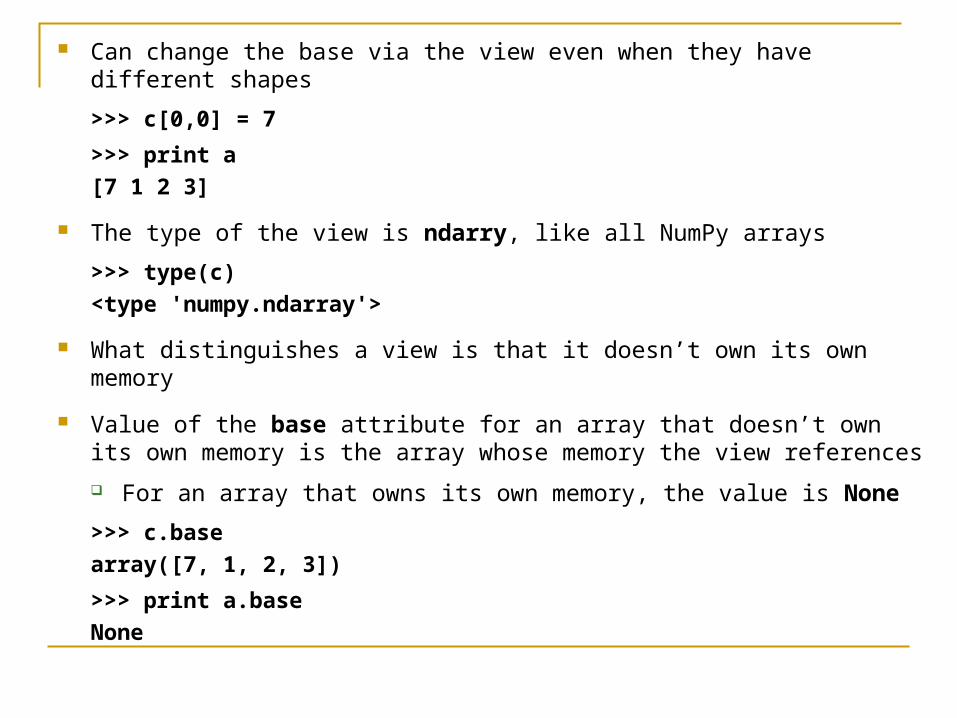
Can change the base via the view even when they have different shapes
>>> c[0,0] = 7
>>> print a
[7 1 2 3]
The type of the view is ndarry, like all NumPy arrays
>>> type(c)
<type 'numpy.ndarray'>
What distinguishes a view is that it doesn’t own its own memory
Value of the base attribute for an array that doesn’t own its own memory is the array whose memory the view references
For an array that owns its own memory, the value is None
>>> c.base
array([7, 1, 2, 3])
>>> print a.base
None
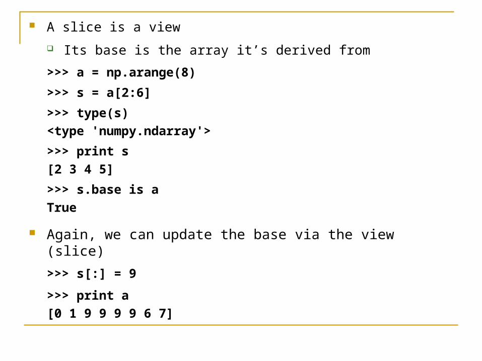
A slice is a view
Its base is the array it’s derived from
>>> a = np.arange(8)
>>> s = a[2:6]
>>> type(s)
<type 'numpy.ndarray'>
>>> print s
[2 3 4 5]
>>> s.base is a
True
Again, we can update the base via the view (slice)
>>> s[:] = 9
>>> print a
[0 1 9 9 9 9 6 7]
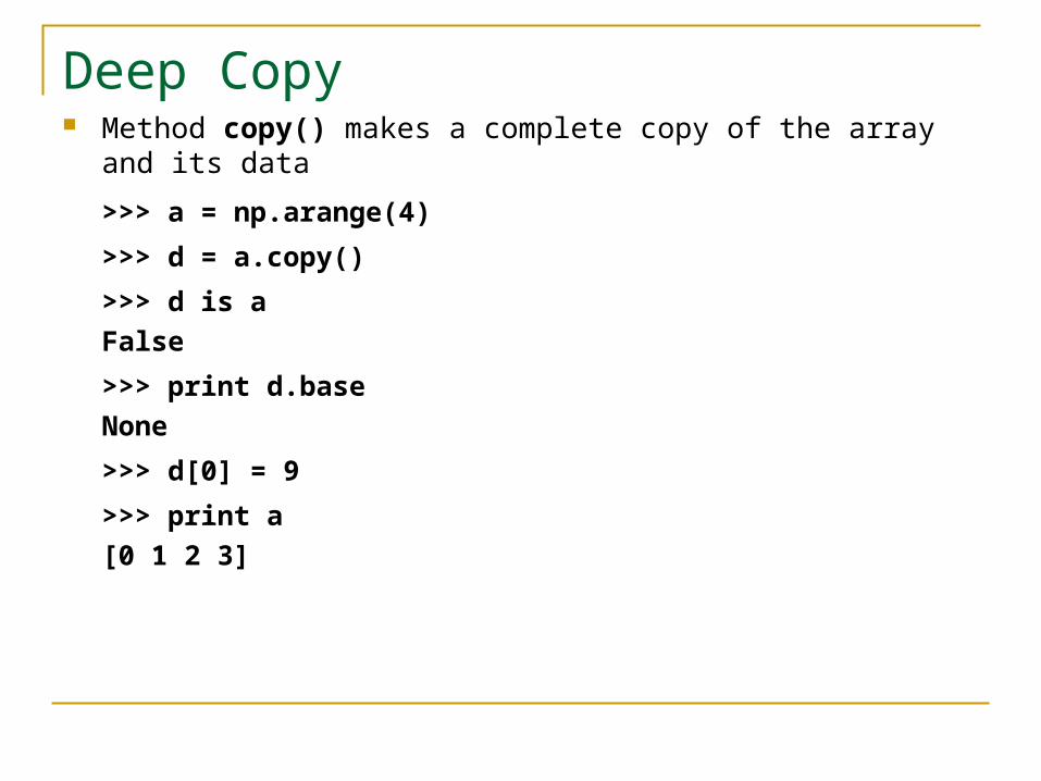
Deep Copy Method copy() makes a complete copy of the array and its data
>>> a = np.arange(4)
>>> d = a.copy()
>>> d is a
False
>>> print d.base
None
>>> d[0] = 9
>>> print a
[0 1 2 3]
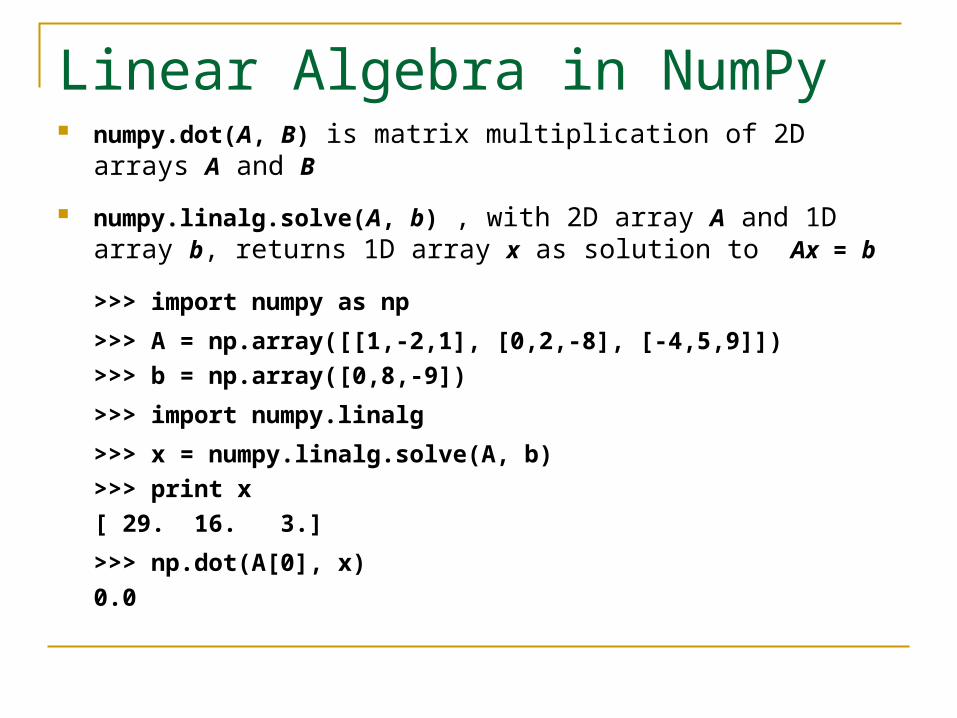
Linear Algebra in NumPy numpy.dot(A, B) is matrix multiplication of 2D arrays A and B
numpy.linalg.solve(A, b) , with 2D array A and 1D array b, returns 1D array x as solution to Ax = b
>>> import numpy as np
>>> A = np.array([[1,-2,1], [0,2,-8], [-4,5,9]])
>>> b = np.array([0,8,-9])
>>> import numpy.linalg
>>> x = numpy.linalg.solve(A, b)
>>> print x
[ 29. 16. 3.]
>>> np.dot(A[0], x)
0.0
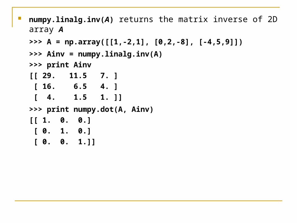
numpy.linalg.inv(A) returns the matrix inverse of 2D array A
>>> A = np.array([[1,-2,1], [0,2,-8], [-4,5,9]])
>>> Ainv = numpy.linalg.inv(A)
>>> print Ainv
[[ 29. 11.5 7. ]
[ 16. 6.5 4. ]
[ 4. 1.5 1. ]]
>>> print numpy.dot(A, Ainv)
[[ 1. 0. 0.]
[ 0. 1. 0.]
[ 0. 0. 1.]]
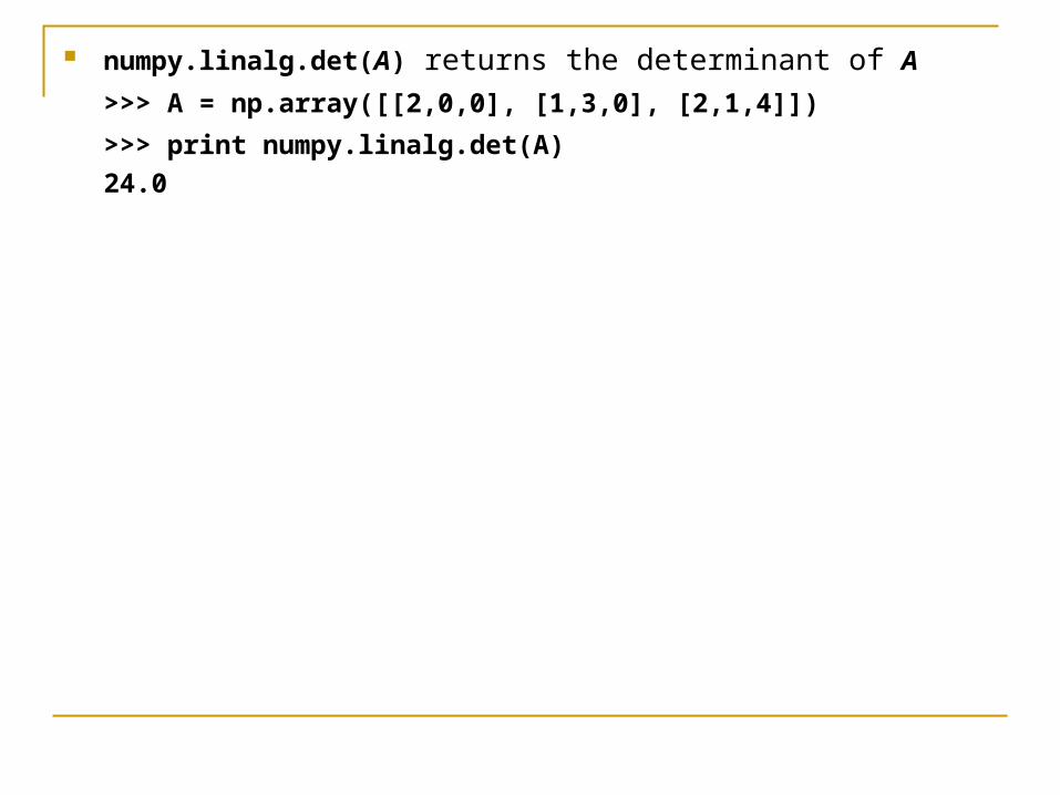
numpy.linalg.det(A) returns the determinant of A
>>> A = np.array([[2,0,0], [1,3,0], [2,1,4]])
>>> print numpy.linalg.det(A)
24.0
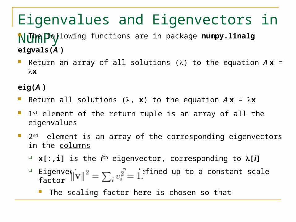
Eigenvalues and Eigenvectors in NumPy The following functions are in package numpy.linalg
eigvals(A )
Return an array of all solutions () to the equation A x = x
eig(A )
Return all solutions (, x) to the equation A x = x
1st element of the return tuple is an array of all the eigenvalues
2nd element is an array of the corresponding eigenvectors in the columns
x[:,i] is the ith eigenvector, corresponding to [i]
Eigenvectors are only defined up to a constant scale factor The scaling factor here is chosen so that
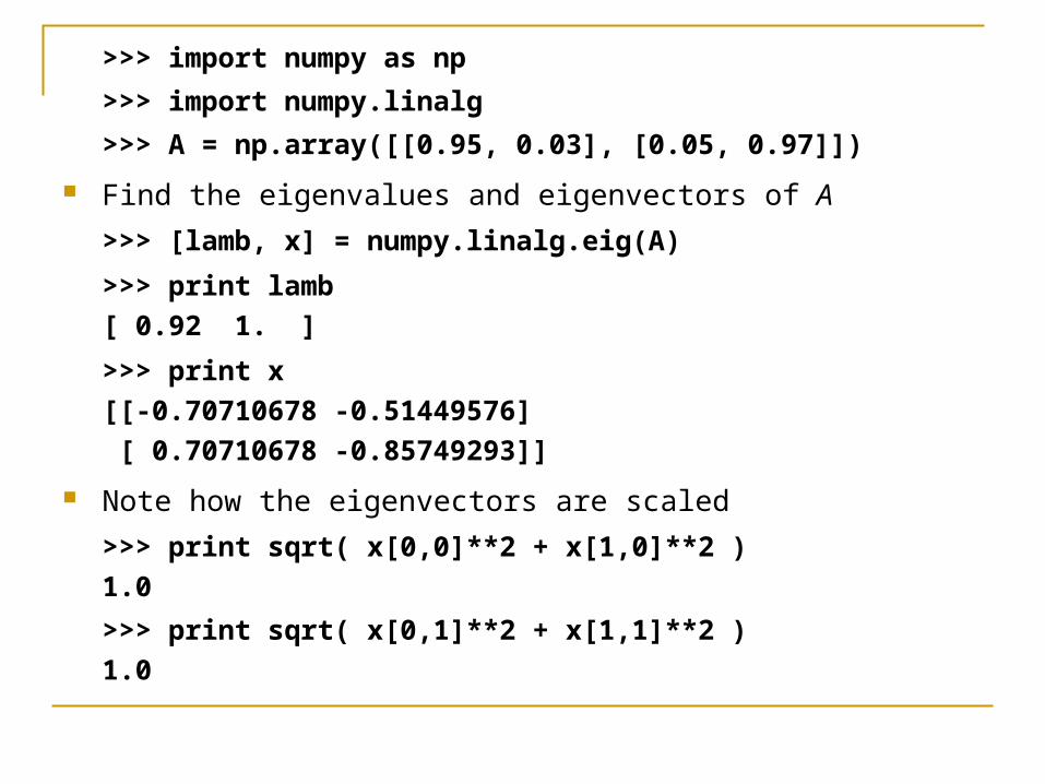
>>> import numpy as np
>>> import numpy.linalg
>>> A = np.array([[0.95, 0.03], [0.05, 0.97]])
Find the eigenvalues and eigenvectors of A
>>> [lamb, x] = numpy.linalg.eig(A)
>>> print lamb
[ 0.92 1. ]
>>> print x
[[-0.70710678 -0.51449576]
[ 0.70710678 -0.85749293]]
Note how the eigenvectors are scaled
>>> print sqrt( x[0,0]**2 + x[1,0]**2 )
1.0
>>> print sqrt( x[0,1]**2 + x[1,1]**2 )
1.0
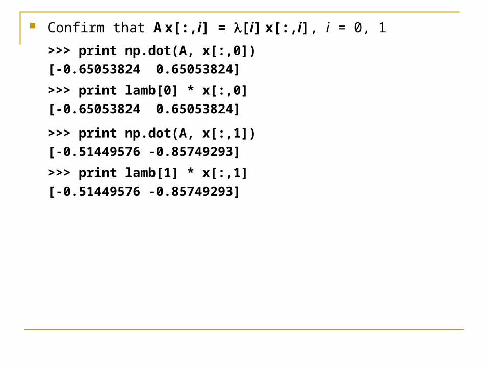
Confirm that A x[:,i] = [i] x[:,i], i = 0, 1
>>> print np.dot(A, x[:,0])
[-0.65053824 0.65053824]
>>> print lamb[0] * x[:,0]
[-0.65053824 0.65053824]
>>> print np.dot(A, x[:,1])
[-0.51449576 -0.85749293]
>>> print lamb[1] * x[:,1]
[-0.51449576 -0.85749293]
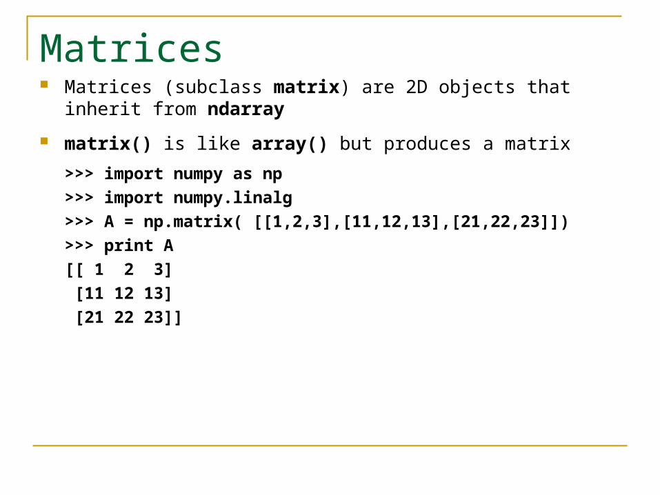
Matrices Matrices (subclass matrix) are 2D objects that inherit from
ndarray
matrix() is like array() but produces a matrix
>>> import numpy as np
>>> import numpy.linalg
>>> A = np.matrix( [[1,2,3],[11,12,13],[21,22,23]])
>>> print A
[[ 1 2 3]
[11 12 13]
[21 22 23]]
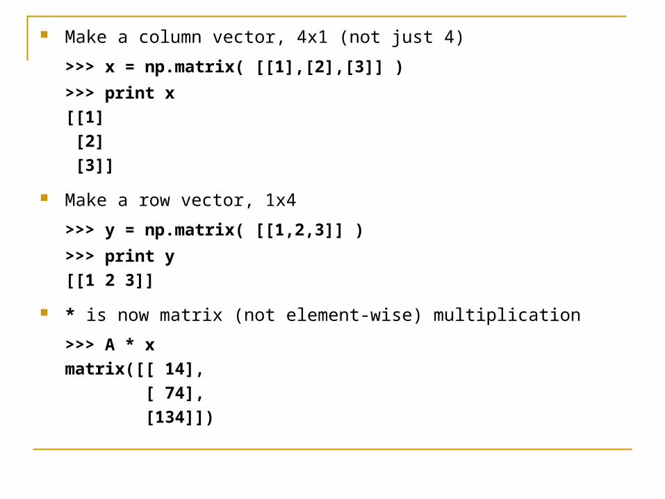
Make a column vector, 4x1 (not just 4)
>>> x = np.matrix( [[1],[2],[3]] )
>>> print x
[[1]
[2]
[3]]
Make a row vector, 1x4
>>> y = np.matrix( [[1,2,3]] )
>>> print y
[[1 2 3]]
* is now matrix (not element-wise) multiplication
>>> A * x
matrix([[ 14],
[ 74],
[134]])
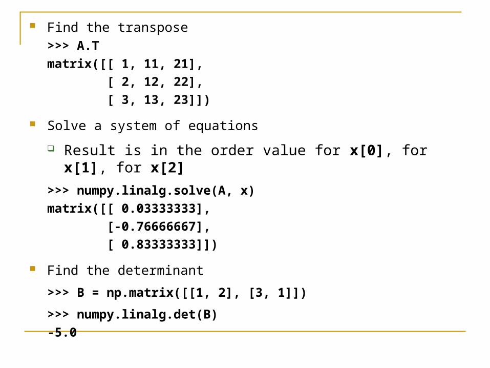
Find the transpose >>> A.T
matrix([[ 1, 11, 21],
[ 2, 12, 22],
[ 3, 13, 23]])
Solve a system of equations
Result is in the order value for x[0], for x[1], for x[2]
>>> numpy.linalg.solve(A, x)
matrix([[ 0.03333333],
[-0.76666667],
[ 0.83333333]])
Find the determinant
>>> B = np.matrix([[1, 2], [3, 1]])
>>> numpy.linalg.det(B)
-5.0
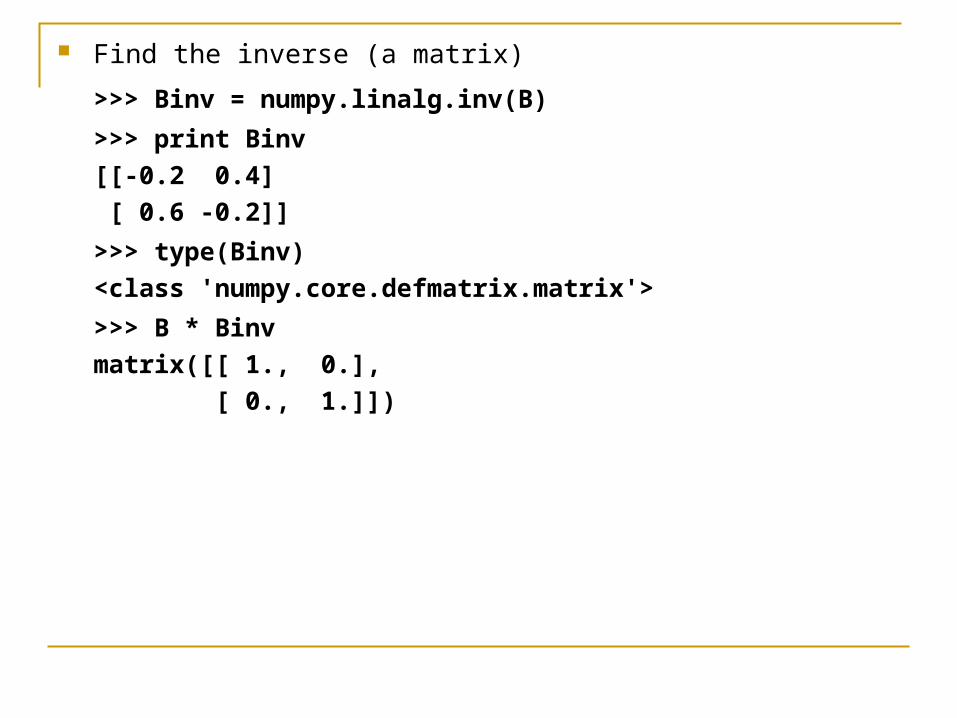
Find the inverse (a matrix)
>>> Binv = numpy.linalg.inv(B)
>>> print Binv
[[-0.2 0.4]
[ 0.6 -0.2]]
>>> type(Binv)
<class 'numpy.core.defmatrix.matrix'>
>>> B * Binv
matrix([[ 1., 0.],
[ 0., 1.]])
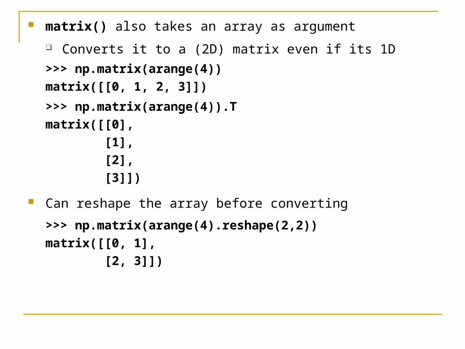
matrix() also takes an array as argument
Converts it to a (2D) matrix even if its 1D
>>> np.matrix(arange(4))
matrix([[0, 1, 2, 3]])
>>> np.matrix(arange(4)).T
matrix([[0],
[1],
[2],
[3]])
Can reshape the array before converting
>>> np.matrix(arange(4).reshape(2,2))
matrix([[0, 1],
[2, 3]])
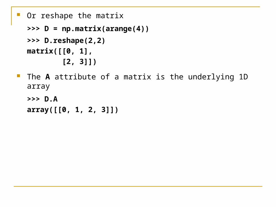
Or reshape the matrix
>>> D = np.matrix(arange(4))
>>> D.reshape(2,2)
matrix([[0, 1],
[2, 3]])
The A attribute of a matrix is the underlying 1D array
>>> D.A
array([[0, 1, 2, 3]])
Can index, slice, and iterate over matrices much as with arrays
The linear algebra package works with both arrays and matrices
It’s generally advisable to use arrays
But you can mix them
E.g., use arrays for the bulk of the code
Switch to matrices when doing lots of multiplication
Recommended