Slide 1
Satellite data assimilation of atmospheric composition
Richard Engelen
Contributions from: Angela Benedetti, Abhishek Chatterjee, Dick Dee,
Steve English, Johannes Flemming, Antje Inness, Johannes Kaiser,
Sebastien Massart, Tony McNally, and Paul Poli
NWP-SAF Training Course Slide 1
Slide 2
NWP-SAF Training Course Slide 2
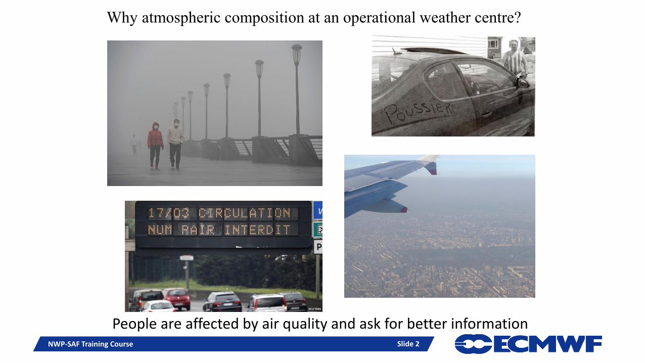
Why atmospheric composition at an operational weather centre?
People are affected by air quality and ask for better information
Slide 3
Why this lecture?
Basic data assimilation theory is the same for atmospheric composition, but…
Radiance assimilation is not always feasible (yet)
Atmospheric composition data assimilation is much more determined by things like emissions and chemistry than by the initial values
With many species not being observed, the problem is even more underdetermined than the standard NWP case
Atmospheric composition impacts the basic NWP problem as well
Slide 3NWP-SAF Training Course
Slide 4
dzdz
dzTBL
0
)())(,()(
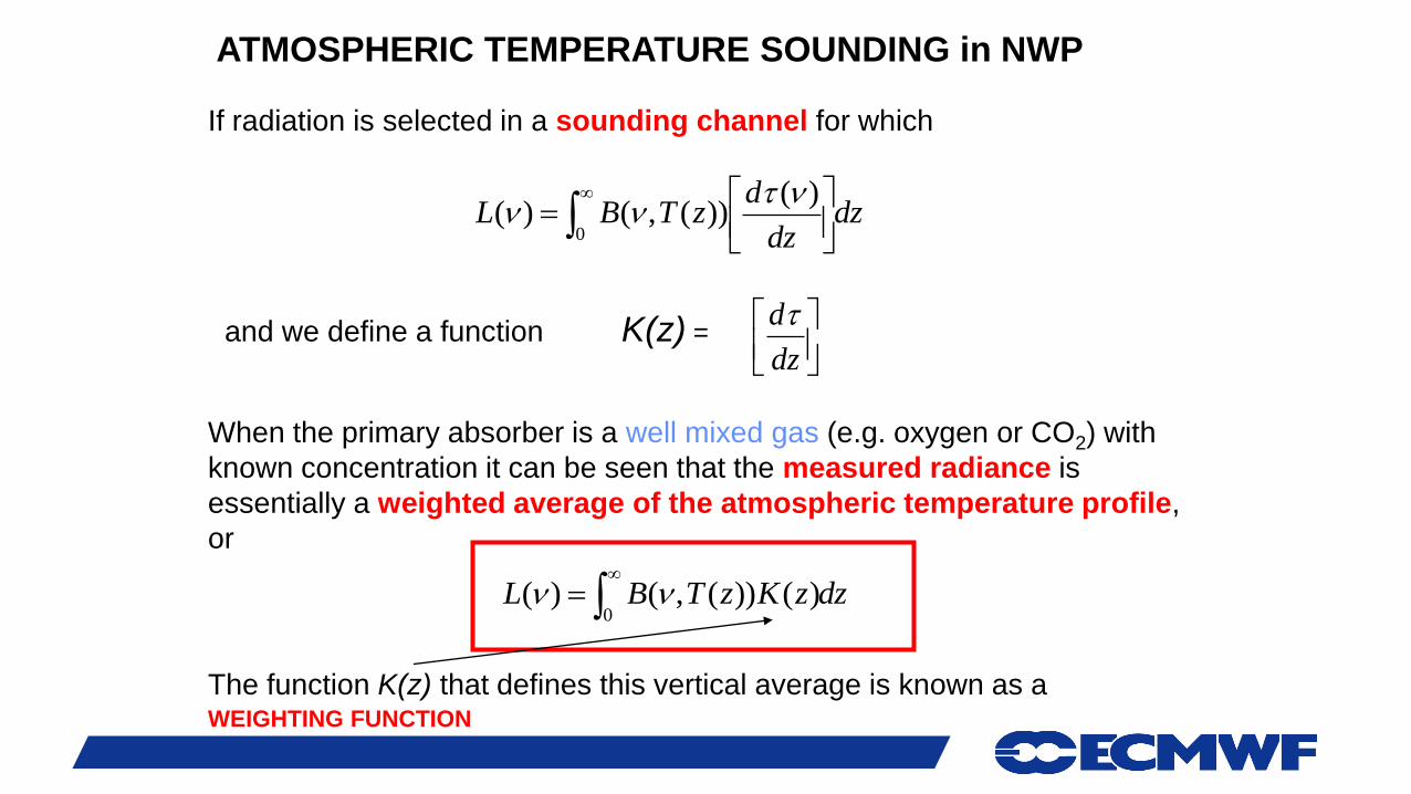
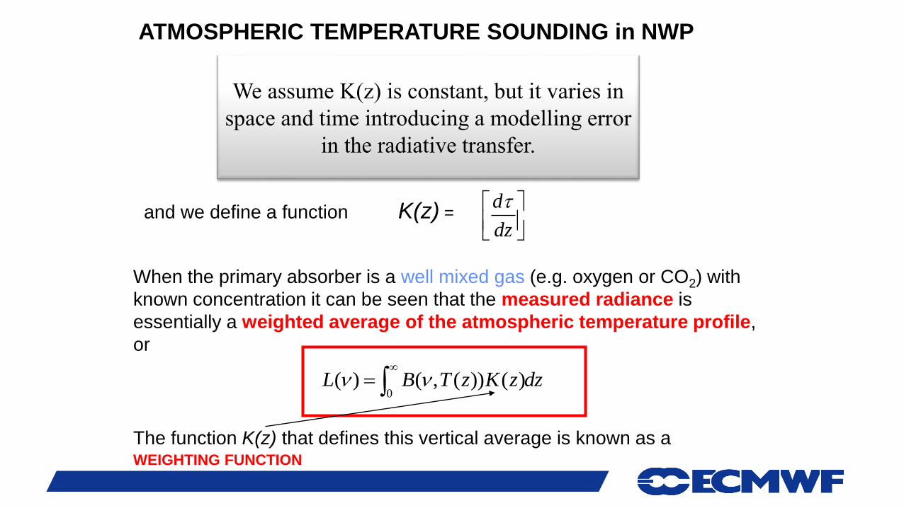
ATMOSPHERIC TEMPERATURE SOUNDING in NWP
If radiation is selected in a sounding channel for which
and we define a function K(z) =
dz
d
When the primary absorber is a well mixed gas (e.g. oxygen or CO2) with
known concentration it can be seen that the measured radiance is
essentially a weighted average of the atmospheric temperature profile,
or
dzzKzTBL
0
)())(,()(
The function K(z) that defines this vertical average is known as a WEIGHTING FUNCTION
Slide 5
NWP-SAF Training Course Slide 5
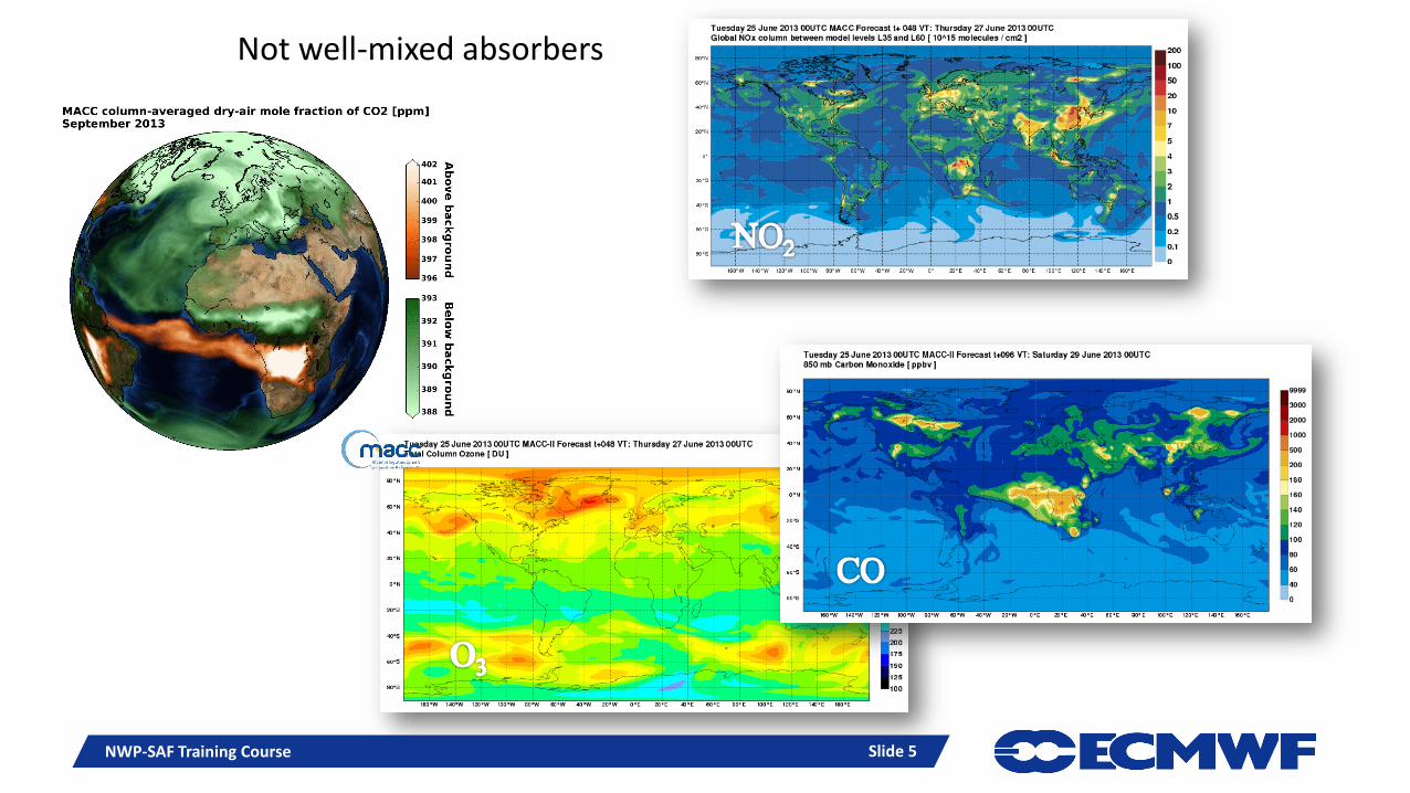
Not well-mixed absorbers
Slide 6
ATMOSPHERIC TEMPERATURE SOUNDING in NWP
and we define a function K(z) =
dz
d
When the primary absorber is a well mixed gas (e.g. oxygen or CO2) with
known concentration it can be seen that the measured radiance is
essentially a weighted average of the atmospheric temperature profile,
or
dzzKzTBL
0
)())(,()(
The function K(z) that defines this vertical average is known as a WEIGHTING FUNCTION
We assume K(z) is constant, but it varies in
space and time introducing a modelling error
in the radiative transfer.
Slide 7
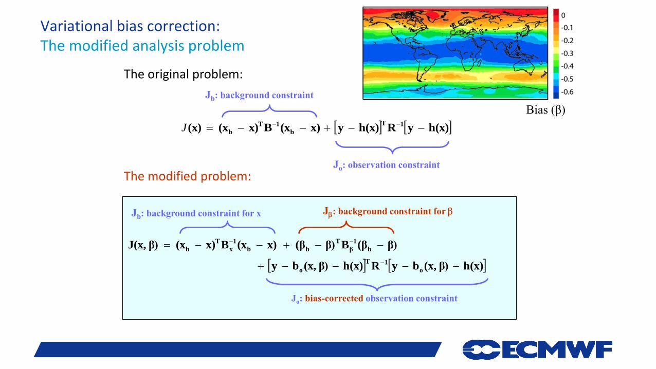
Variational bias correction: The modified analysis problem
Jb: background constraint
Jo: observation constraint
h(x)yRh(x)yx)(xBx)(x(x)1T
b
1T
b J
The original problem:
h(x)β)(x,byRh(x)β)(x,by
β)(βBβ)(βx)(xBx)(xβ)J(x,
o
1T
o
b
1
β
T
bb
1
x
T
b
Jb: background constraint for x J: background constraint for
Jo: bias-corrected observation constraint
The modified problem:
Bias (β)
Slide 8
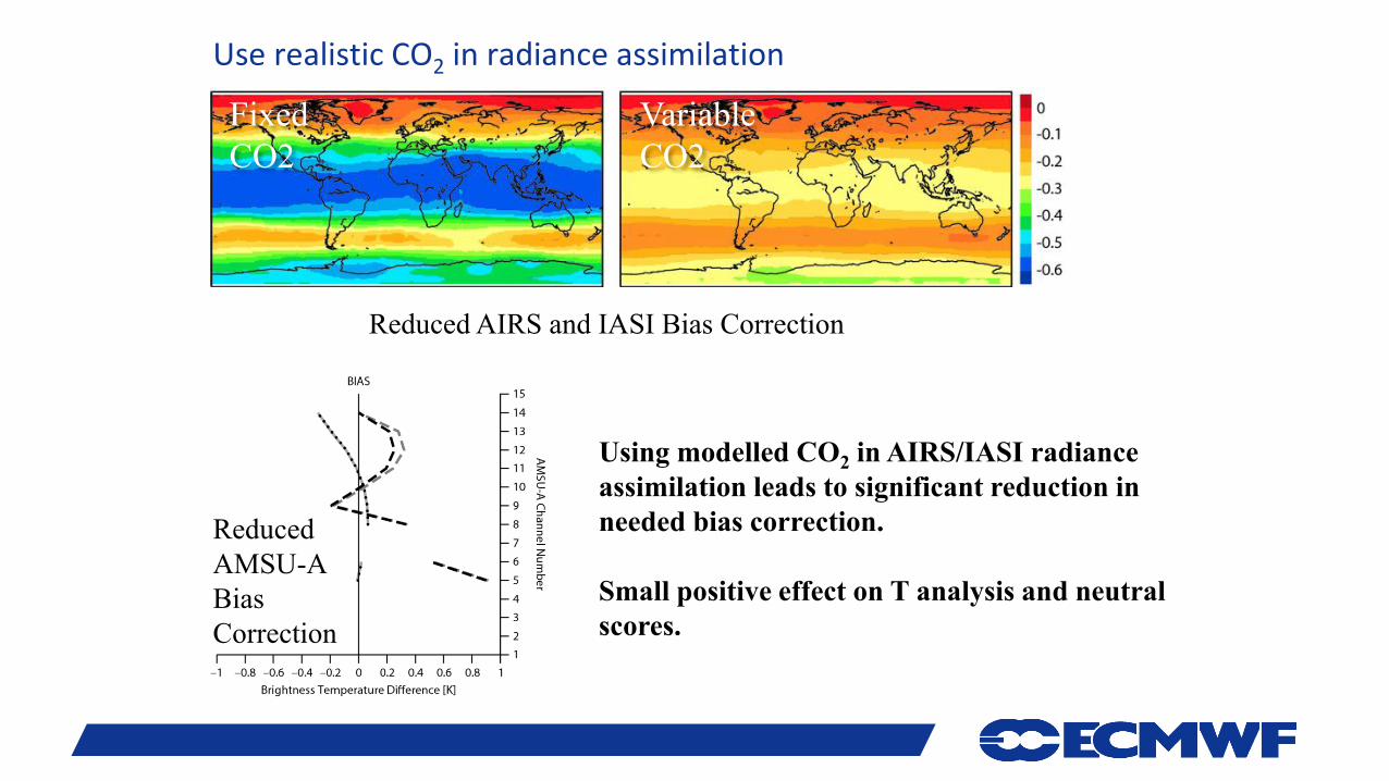
Use realistic CO2 in radiance assimilation
Using modelled CO2 in AIRS/IASI radiance
assimilation leads to significant reduction in
needed bias correction.
Small positive effect on T analysis and neutral
scores.
Reduced
AMSU-A
Bias
Correction
Reduced AIRS and IASI Bias Correction
Fixed
CO2
Variable
CO2
Slide 9
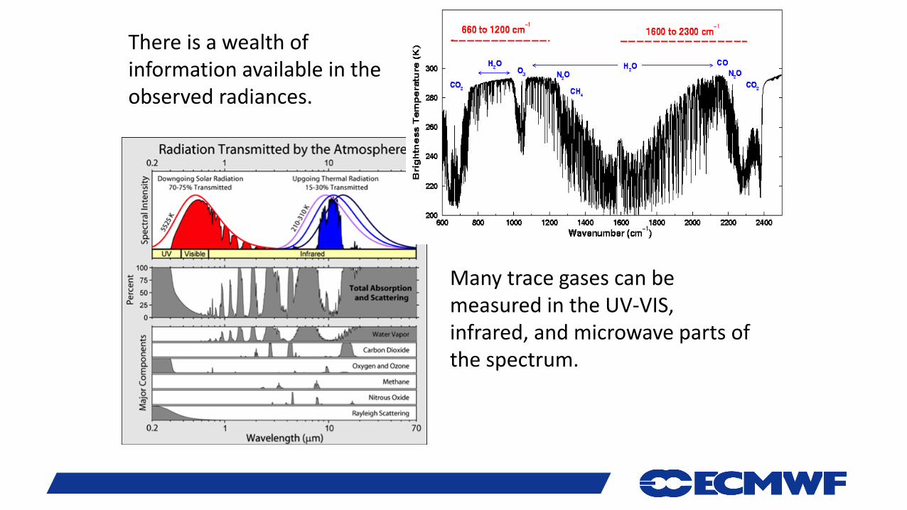
Many trace gases can be measured in the UV-VIS, infrared, and microwave parts of the spectrum.
There is a wealth of information available in the observed radiances.
Slide 10
NWP-SAF Training Course Slide 10
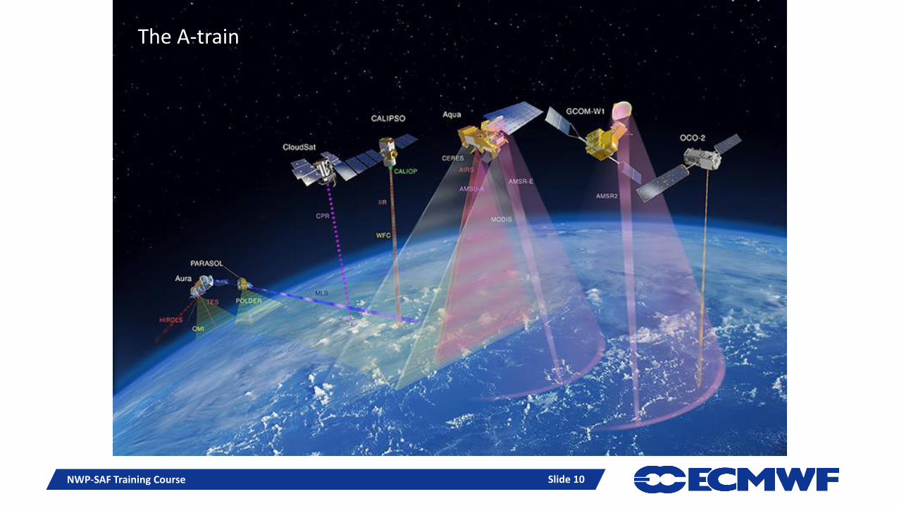
The A-train
Slide 11
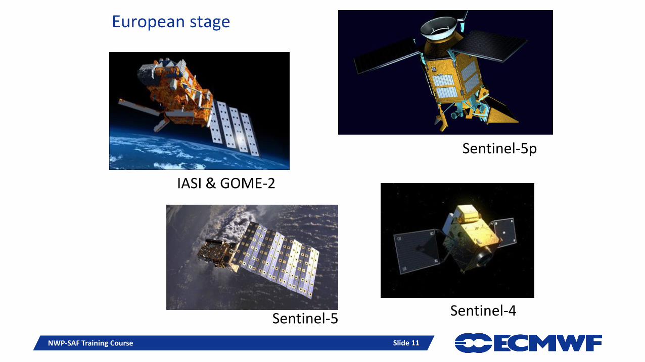
European stage
NWP-SAF Training Course Slide 11
Sentinel-5p
Sentinel-4Sentinel-5
IASI & GOME-2
Slide 12
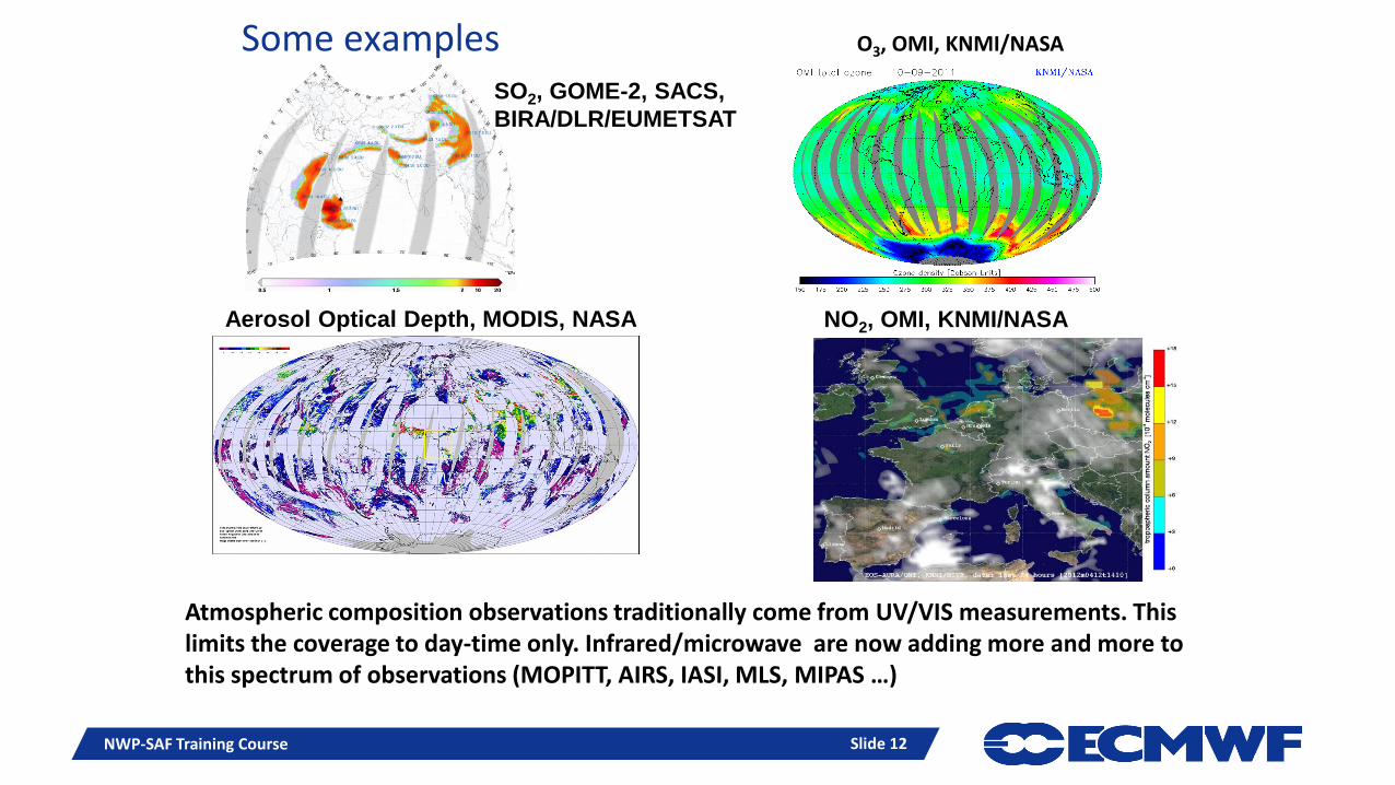
SO2, GOME-2, SACS,
BIRA/DLR/EUMETSAT
NO2, OMI, KNMI/NASAAerosol Optical Depth, MODIS, NASA
Some examples O3, OMI, KNMI/NASA
Atmospheric composition observations traditionally come from UV/VIS measurements. This limits the coverage to day-time only. Infrared/microwave are now adding more and more to this spectrum of observations (MOPITT, AIRS, IASI, MLS, MIPAS …)
NWP-SAF Training Course Slide 12
Slide 13
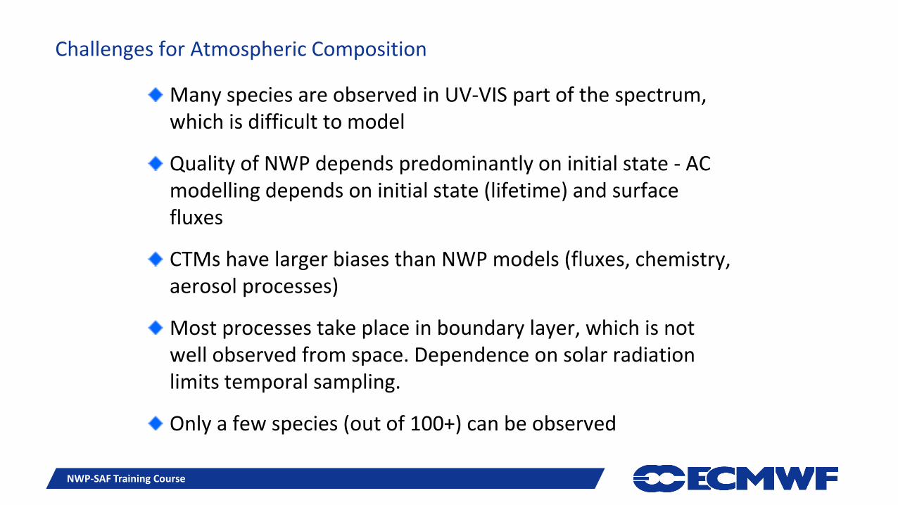
Challenges for Atmospheric Composition
Many species are observed in UV-VIS part of the spectrum, which is difficult to model
Quality of NWP depends predominantly on initial state - AC modelling depends on initial state (lifetime) and surface fluxes
CTMs have larger biases than NWP models (fluxes, chemistry, aerosol processes)
Most processes take place in boundary layer, which is not well observed from space. Dependence on solar radiation limits temporal sampling.
Only a few species (out of 100+) can be observed
NWP-SAF Training Course
Slide 14
RADIANCES VS. RETRIEVALS
NWP-SAF Training Course Slide 14
Slide 15
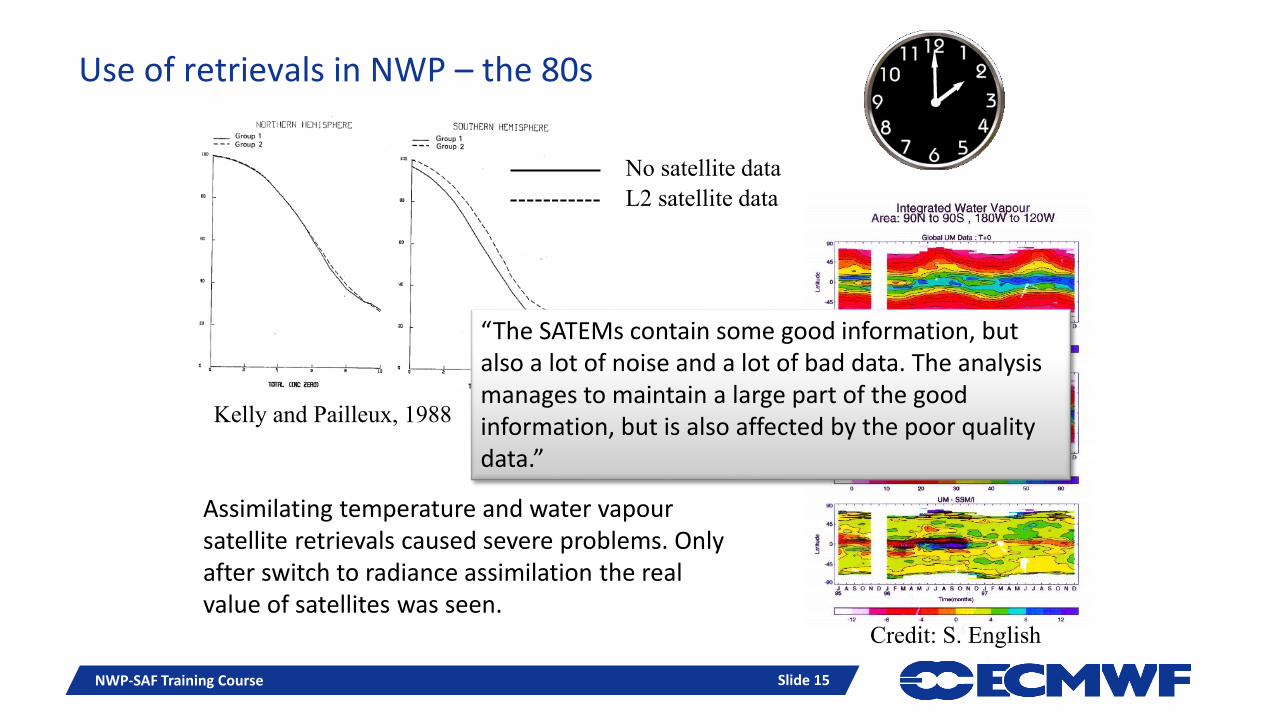
Use of retrievals in NWP – the 80s
NWP-SAF Training Course Slide 15
Kelly and Pailleux, 1988
Assimilating temperature and water vapour satellite retrievals caused severe problems. Only after switch to radiance assimilation the real value of satellites was seen.
“The SATEMs contain some good information, but also a lot of noise and a lot of bad data. The analysis manages to maintain a large part of the good information, but is also affected by the poor quality data.”
Credit: S. English
No satellite data
L2 satellite data
Slide 16
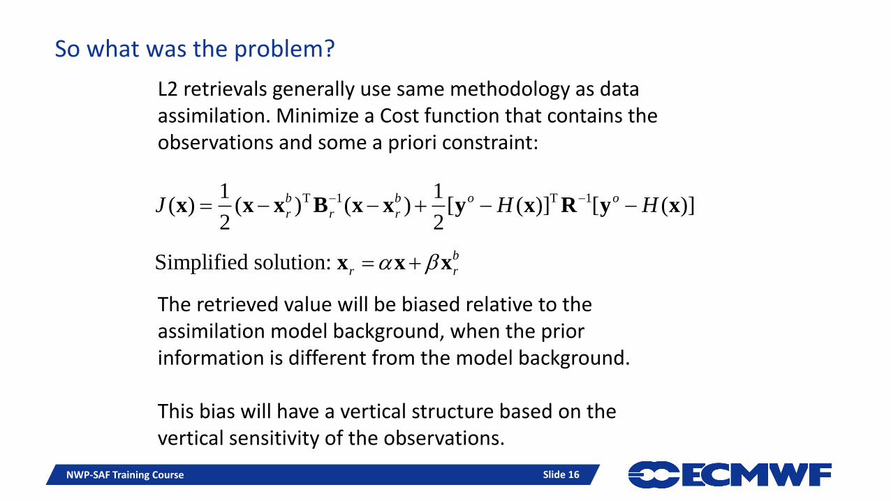
So what was the problem?
NWP-SAF Training Course Slide 16
T 1 T 11 1( ) ( ) ( ) [ ( )] [ ( )]
2 2
b b o o
r r rJ H H x x x B x x y x R y x
L2 retrievals generally use same methodology as data assimilation. Minimize a Cost function that contains the observations and some a priori constraint:
The retrieved value will be biased relative to the assimilation model background, when the prior information is different from the model background.
This bias will have a vertical structure based on the vertical sensitivity of the observations.
Simplified solution: b
r r x x x
Slide 17
1
1 1
1
T
r
T
r
S K R K B
A S K R K
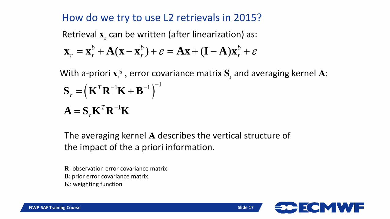
How do we try to use L2 retrievals in 2015?
Slide 17
( ) ( )b b b
r r r r x x A x x Ax I A x
The averaging kernel A describes the vertical structure of the impact of the a priori information.
R: observation error covariance matrixB: prior error covariance matrixK: weighting function
Retrieval xr can be written (after linearization) as:
With a-priori xrb , error covariance matrix Sr and averaging kernel A:
NWP-SAF Training Course
Slide 18
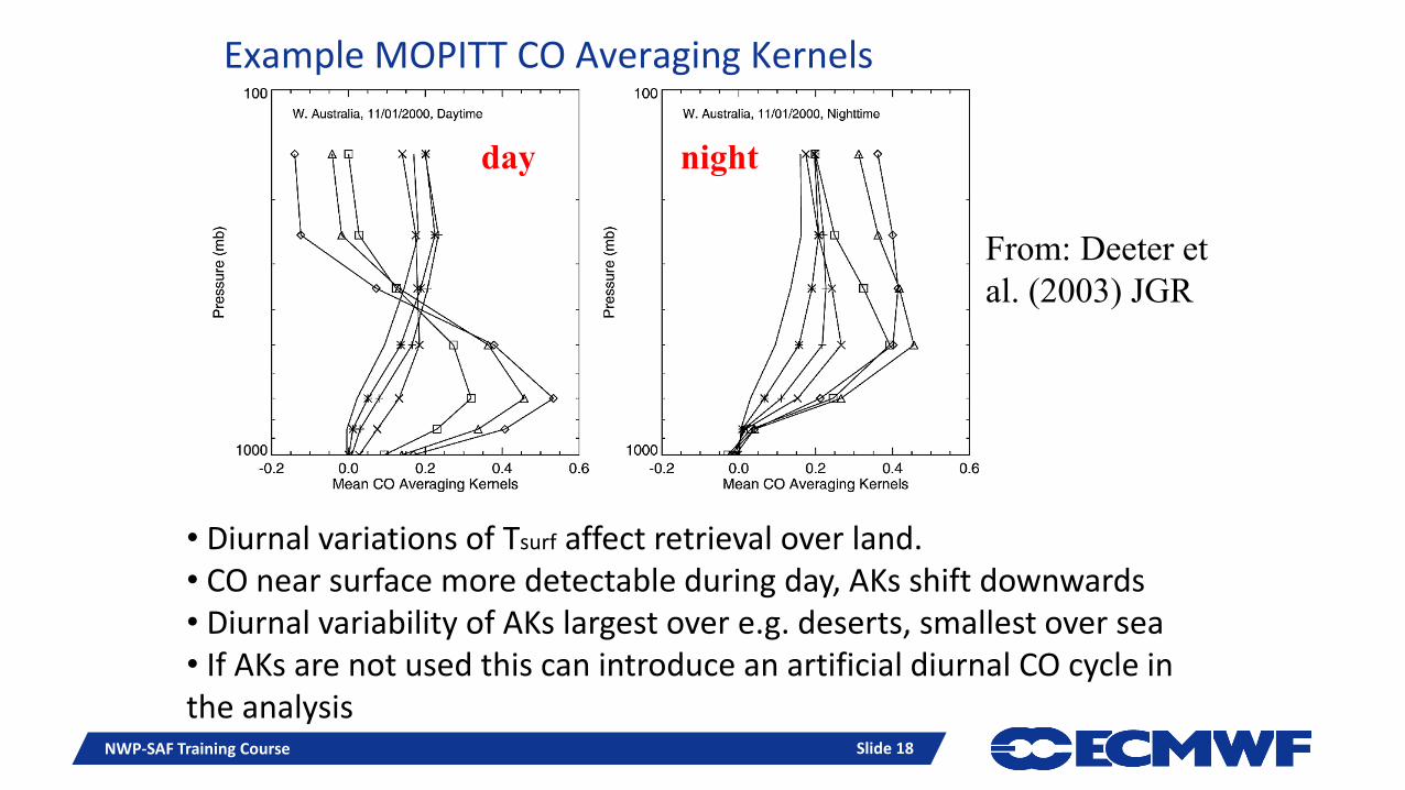
Example MOPITT CO Averaging Kernels
Slide 18
From: Deeter et
al. (2003) JGR
NWP-SAF Training Course
• Diurnal variations of Tsurf affect retrieval over land.• CO near surface more detectable during day, AKs shift downwards • Diurnal variability of AKs largest over e.g. deserts, smallest over sea• If AKs are not used this can introduce an artificial diurnal CO cycle in the analysis
day night
Slide 19
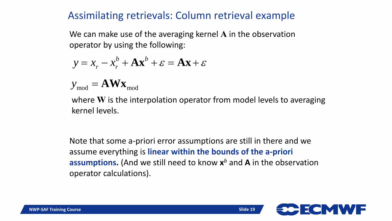
Assimilating retrievals: Column retrieval example
Slide 19
We can make use of the averaging kernel A in the observation operator by using the following:
Note that some a-priori error assumptions are still in there and we assume everything is linear within the bounds of the a-priori assumptions. (And we still need to know xb and A in the observation operator calculations).
NWP-SAF Training Course
b b
r ry x x Ax Ax
mod mody AWx
where W is the interpolation operator from model levels to averaging kernel levels.
Slide 20
Assimilating retrievals: summary
NWP-SAF Training Course Slide 20
• Retrieval teams can focus their expertise fully on specific observation
• Good communication between data providers and data assimilation users needed
• Good characterization of retrieval is crucial• Averaging kernels• A priori• Error estimates• Quality flags

Slide 21
INITIAL VS. BOUNDARY VALUES
NWP-SAF Training Course Slide 21
Slide 22
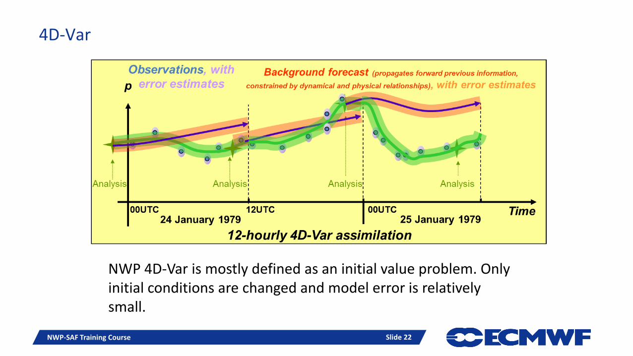
4D-Var
NWP-SAF Training Course Slide 22
NWP 4D-Var is mostly defined as an initial value problem. Only initial conditions are changed and model error is relatively small.
Slide 23
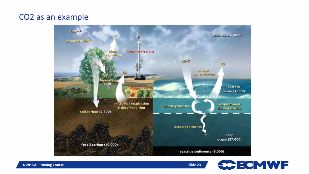
CO2 as an example
NWP-SAF Training Course Slide 23
Slide 24
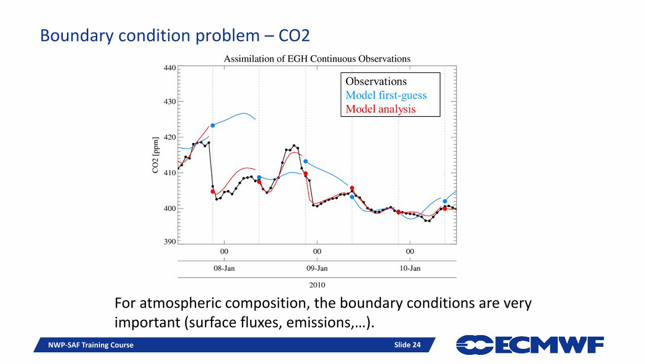
Boundary condition problem – CO2
NWP-SAF Training Course Slide 24
For atmospheric composition, the boundary conditions are very important (surface fluxes, emissions,…).
Slide 25
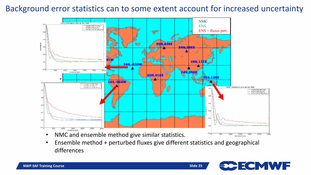
Background error statistics can to some extent account for increased uncertaintyNMC
ENS
ENS + fluxes pert.
• NMC and ensemble method give similar statistics.• Ensemble method + perturbed fluxes give different statistics and geographical
differences
NWP-SAF Training Course Slide 25
Slide 26
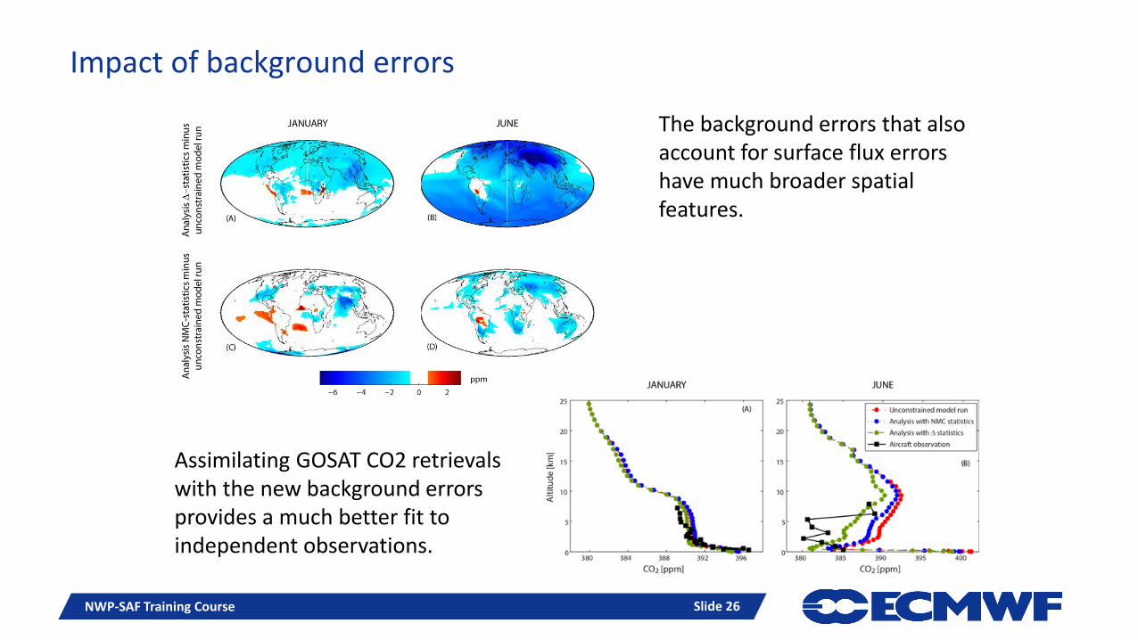
Impact of background errors
NWP-SAF Training Course Slide 26
The background errors that also account for surface flux errors have much broader spatial features.
Assimilating GOSAT CO2 retrievals with the new background errors provides a much better fit to independent observations.
Slide 27
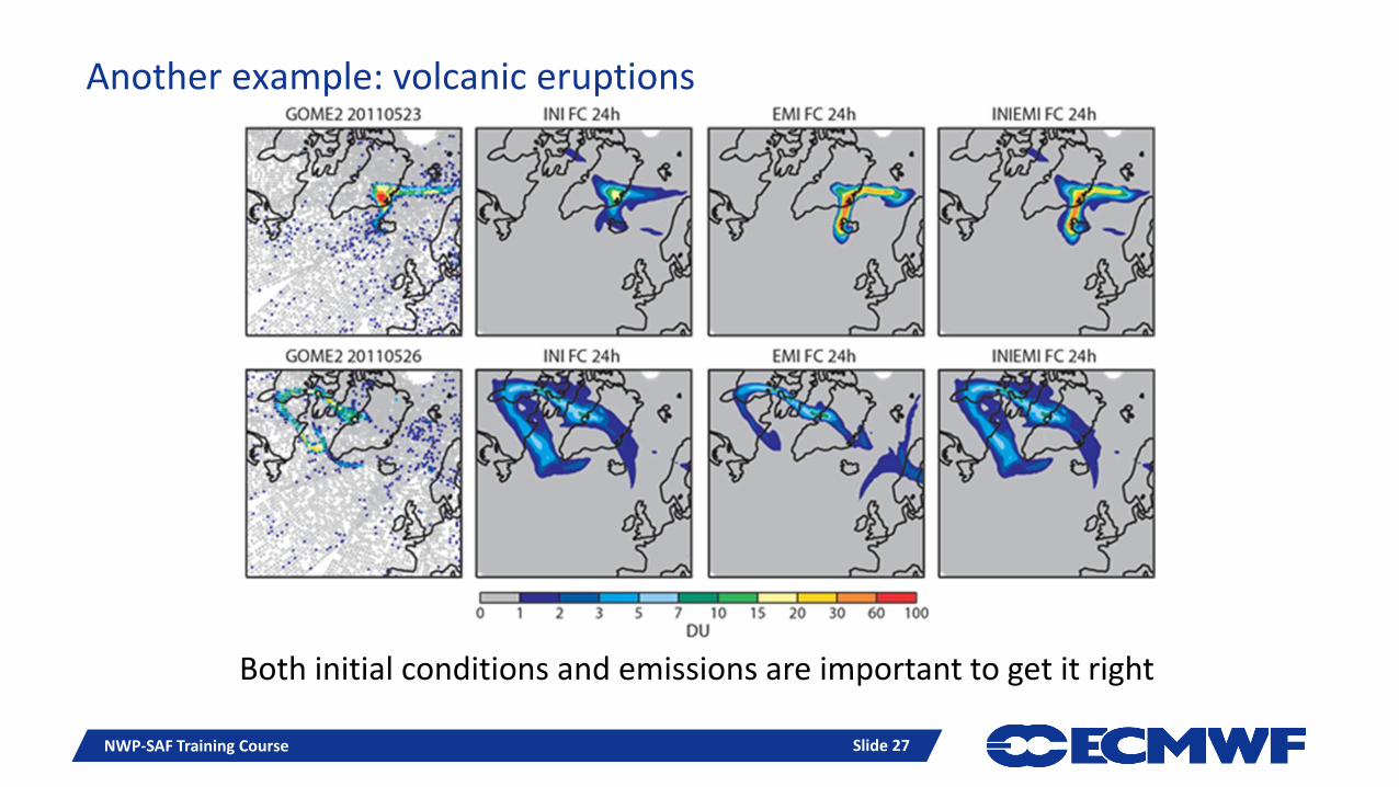
Another example: volcanic eruptions
NWP-SAF Training Course Slide 27
Both initial conditions and emissions are important to get it right
Slide 28
Current research developments
NWP-SAF Training Course Slide 28
• Use (data constrained) models for surface fluxes• Use of CTESSEL land carbon model in ECMWF/MACC
CO2 model
• Add flux increments to the assimilation control vector• Already tested in LETKF by Kang et al. with promising
results
• Use satellite observed flux estimates in DA system • Use of GFAS fire detection method at ECMWF
Slide 29
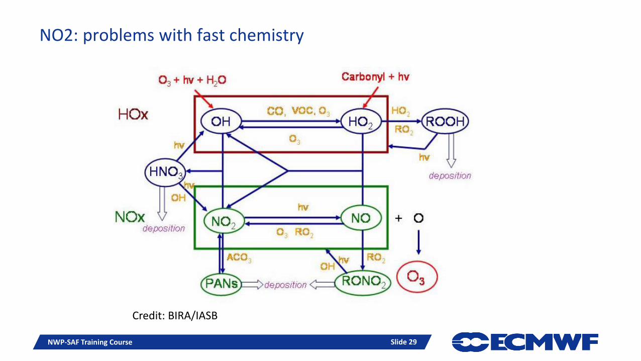
NO2: problems with fast chemistry
NWP-SAF Training Course Slide 29
Credit: BIRA/IASB
Slide 30
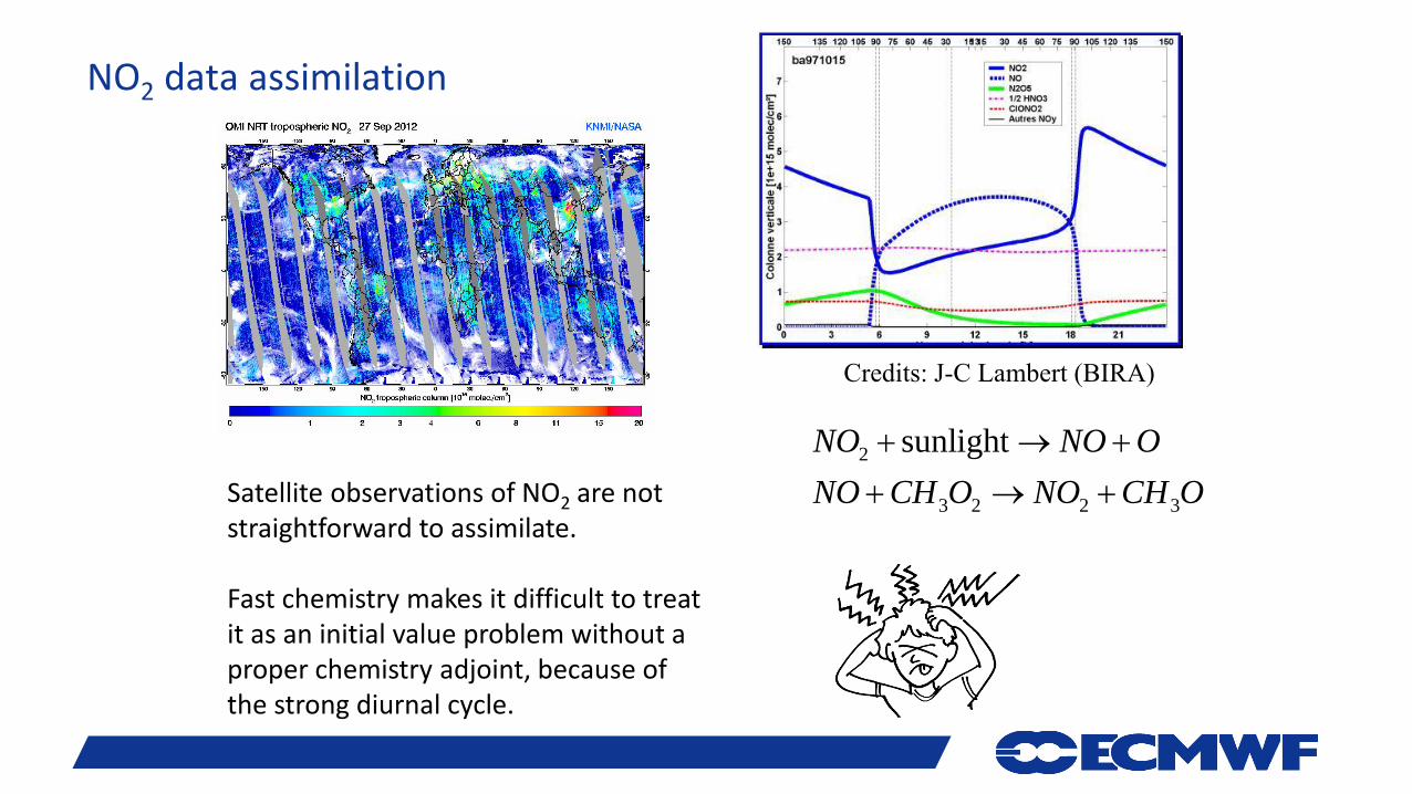
NO2 data assimilation
Satellite observations of NO2 are not straightforward to assimilate.
Fast chemistry makes it difficult to treat it as an initial value problem without a proper chemistry adjoint, because of the strong diurnal cycle.
Credits: J-C Lambert (BIRA)
2
3 2 2 3
sunlightNO NO O
NO CH O NO CH O
Slide 31
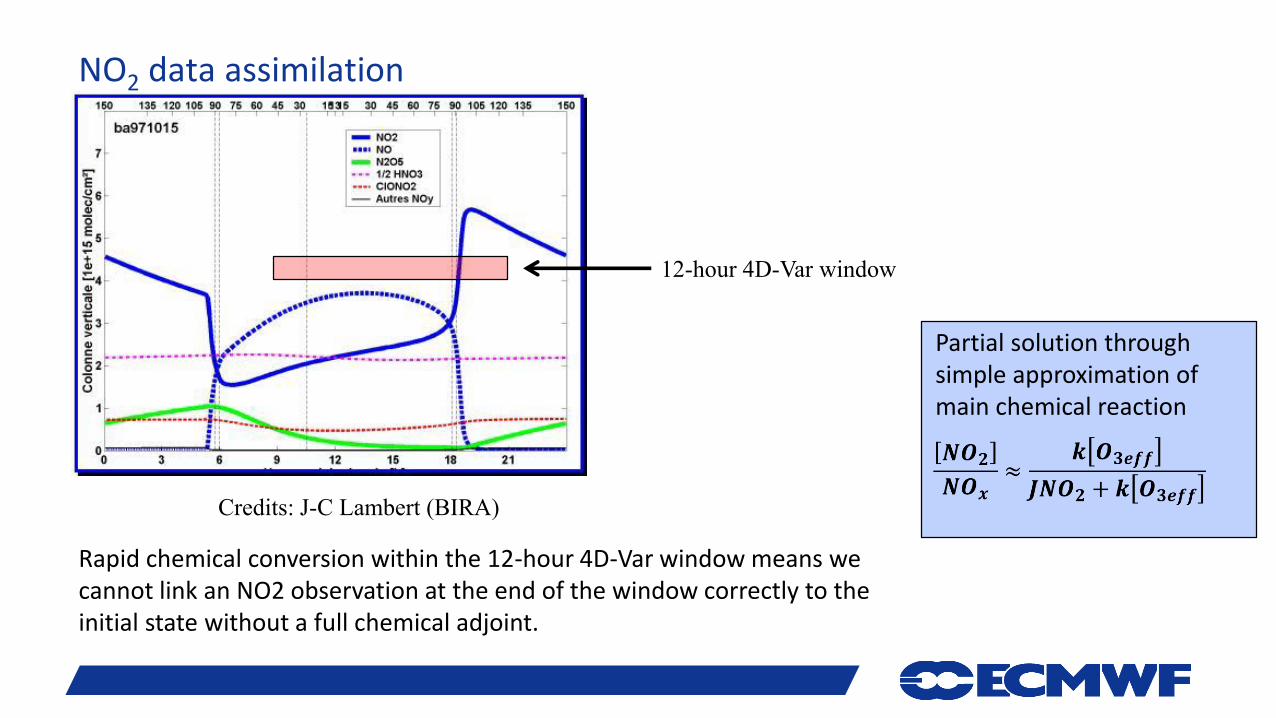
NO2 data assimilation
Credits: J-C Lambert (BIRA)
12-hour 4D-Var window
Rapid chemical conversion within the 12-hour 4D-Var window means we cannot link an NO2 observation at the end of the window correctly to the initial state without a full chemical adjoint.
Partial solution through simple approximation of main chemical reaction
Slide 32
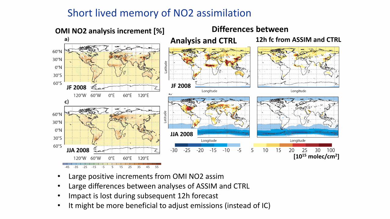
Short lived memory of NO2 assimilation
OMI NO2 analysis increment [%] Differences between
[1015 molec/cm2]
JF 2008
JJA 2008
JF 2008
JJA 2008
• Large positive increments from OMI NO2 assim• Large differences between analyses of ASSIM and CTRL• Impact is lost during subsequent 12h forecast• It might be more beneficial to adjust emissions (instead of IC)
12h fc from ASSIM and CTRLAnalysis and CTRL

Slide 33
SAMPLING ISSUES
NWP-SAF Training Course Slide 33
Slide 34
Issues with Observations
Little or no vertical information from satellite observations. Total or partial columns retrieved from radiation measurements. Weak or no signal from boundary layer.
Fixed overpass times and daylight conditions only (UV-VIS) -> no daily maximum/cycle
Global coverage in a few days (LEO); often limited to cloud free conditions; fixed overpass time.
Retrieval errors can be large; small scales not resolved
NWP-SAF Training Course Slide 34
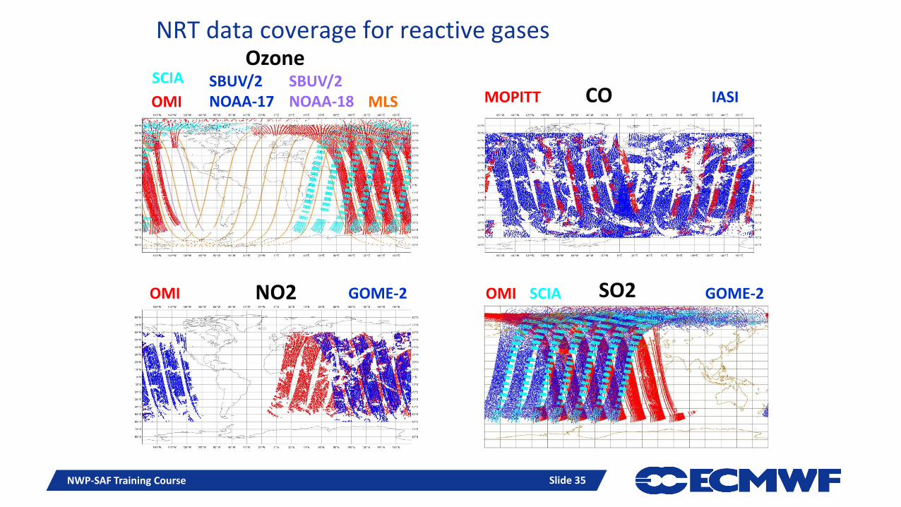
Slide 35
OMISBUV/2 NOAA-17
SBUV/2 NOAA-18 MLS
SCIAMOPITT IASI
GOME-2OMI
Ozone
CO
NO2 GOME-2OMI SO2SCIA
NRT data coverage for reactive gases
NWP-SAF Training Course Slide 35
Slide 36
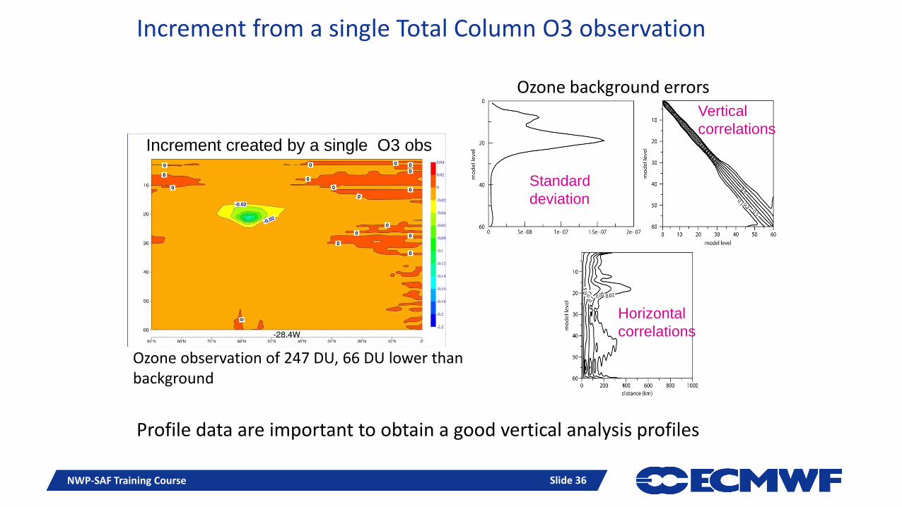
Increment created by a single O3 obs
Increment from a single Total Column O3 observation
Profile data are important to obtain a good vertical analysis profiles
Horizontal
correlations
Standard
deviation
Vertical
correlations
Ozone background errors
Ozone observation of 247 DU, 66 DU lower than background
NWP-SAF Training Course Slide 36
Slide 37
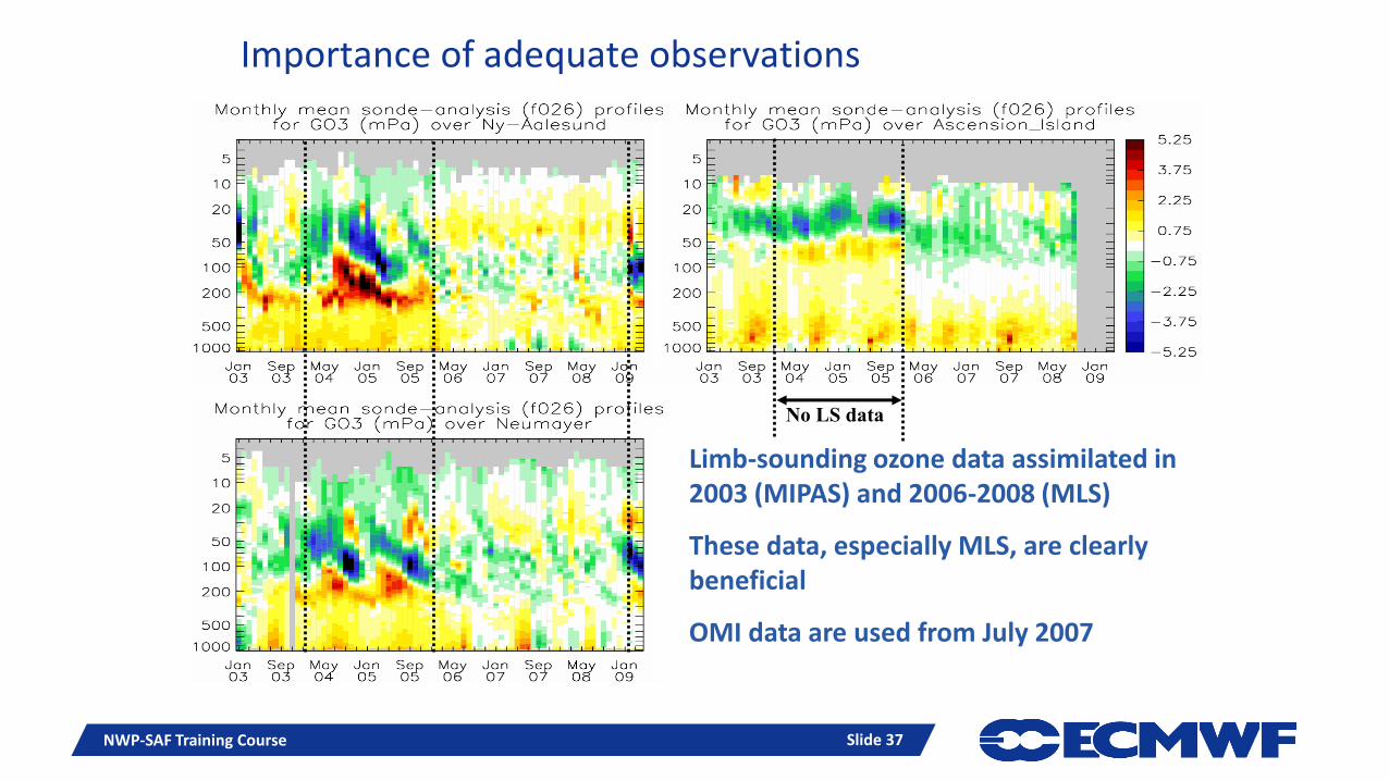
Limb-sounding ozone data assimilated in 2003 (MIPAS) and 2006-2008 (MLS)
These data, especially MLS, are clearly beneficial
OMI data are used from July 2007
No LS data
Importance of adequate observations
NWP-SAF Training Course Slide 37

Slide 38
ONLY A FEW SPECIES ARE OBSERVED
NWP-SAF Training Course Slide 38
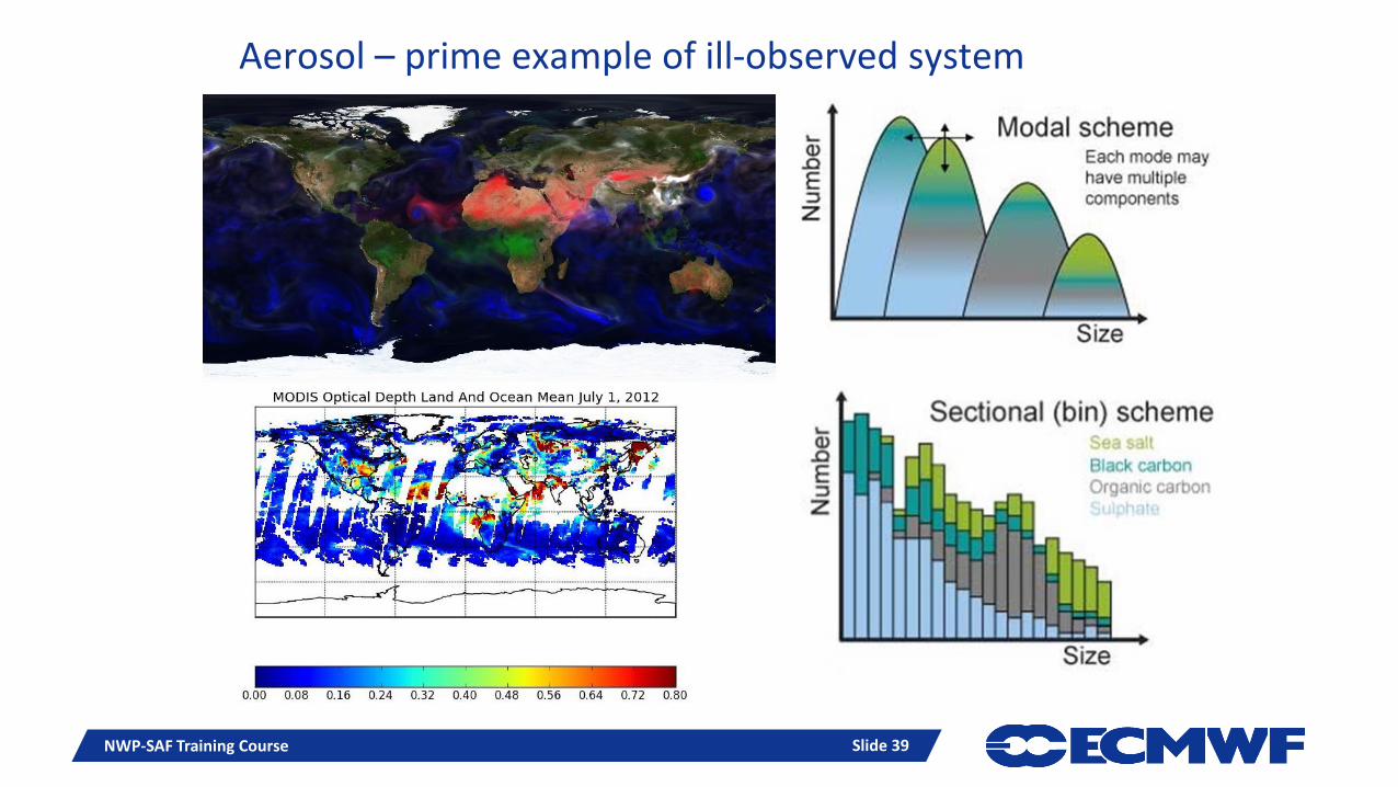
Slide 39
Aerosol – prime example of ill-observed system
NWP-SAF Training Course Slide 39
Slide 40
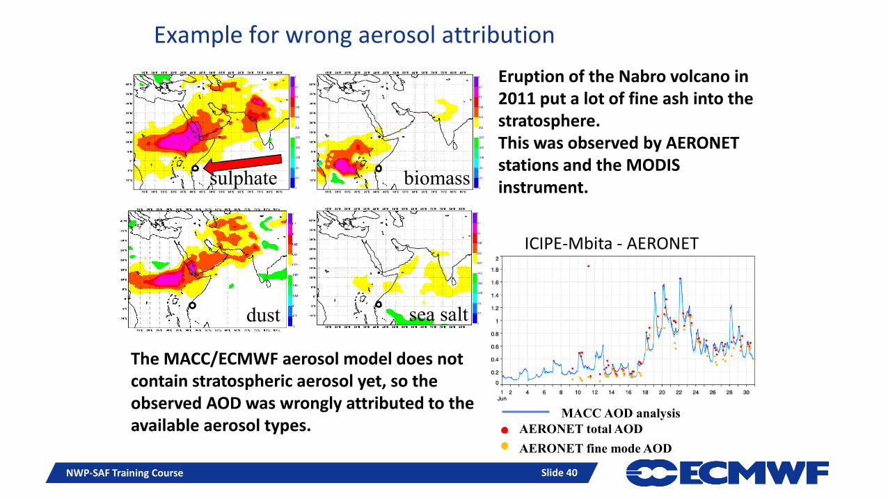
Example for wrong aerosol attribution
sulphate biomass
dust sea salt
Eruption of the Nabro volcano in 2011 put a lot of fine ash into the stratosphere.This was observed by AERONET stations and the MODIS instrument.
The MACC/ECMWF aerosol model does not contain stratospheric aerosol yet, so the observed AOD was wrongly attributed to the available aerosol types.
MACC AOD analysis
AERONET fine mode AOD
ICIPE-Mbita - AERONET
AERONET total AOD
NWP-SAF Training Course Slide 40
Slide 41
Constraining aerosol
NWP-SAF Training Course Slide 41
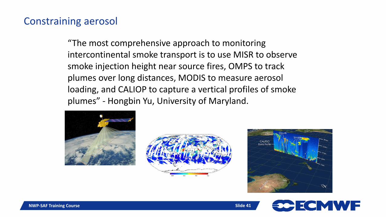
“The most comprehensive approach to monitoring intercontinental smoke transport is to use MISR to observe smoke injection height near source fires, OMPS to track plumes over long distances, MODIS to measure aerosol loading, and CALIOP to capture a vertical profiles of smoke plumes” - Hongbin Yu, University of Maryland.
Slide 42
Unconstrained chemistry
NWP-SAF Training Course Slide 42
Only a small subset of all chemical species is observed from satellites. Most commonly routinely observed are O3, NO2, SO2, CO, HCHO, but some other species are available as well.
Adjoint of chemistry code is not straightforward and not commonly used at the moment. This means that the chemical balance can be disturbed by only changing a few species of the total set in the chemistry scheme.
Slide 43
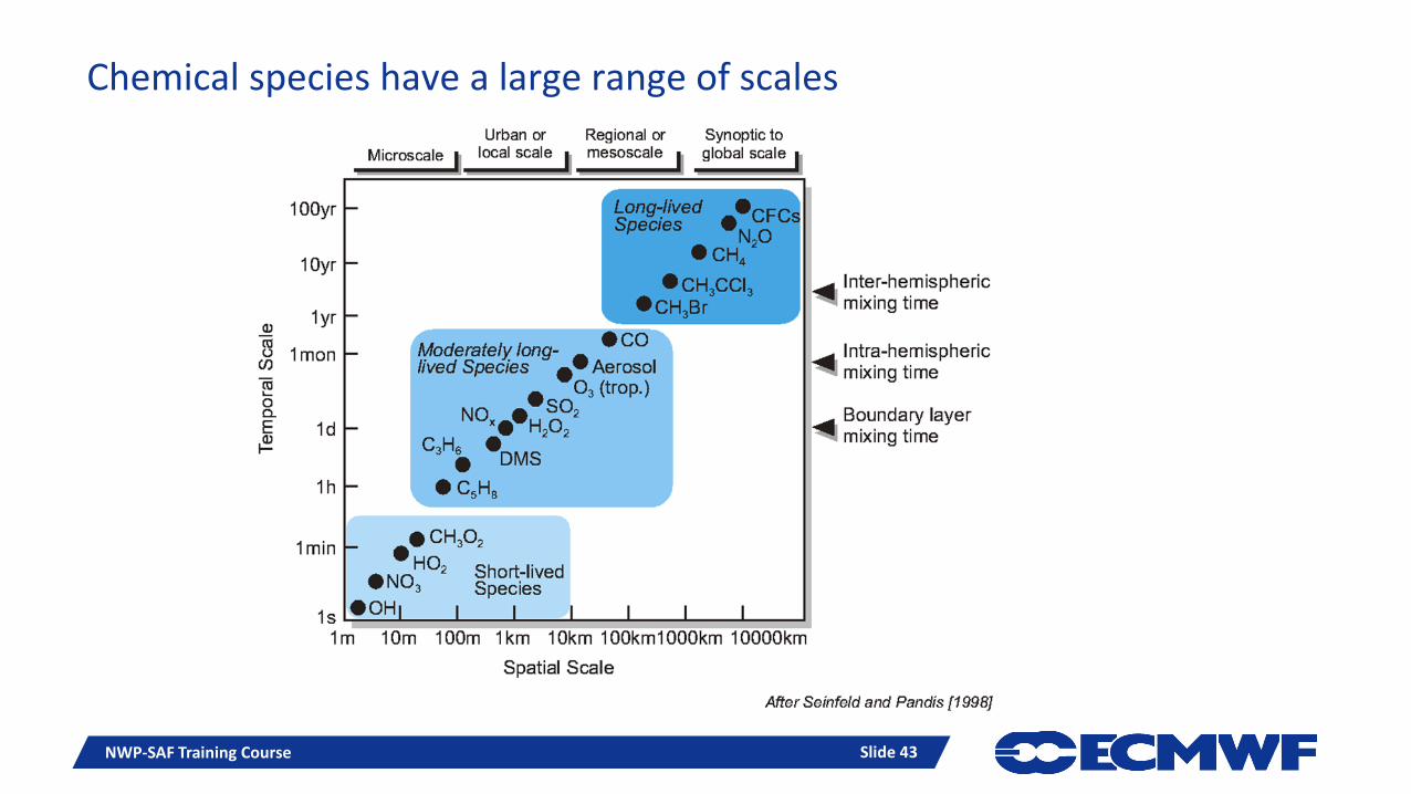
Chemical species have a large range of scales
NWP-SAF Training Course Slide 43
Slide 44
Sampling in summary
Poor sampling in space, time, and species creates problems
Large dependence on model (chemistry, fluxes, species)
Large dependence on correct background errors
Large variety of different satellite observations needed to better constrain the problem
Slide 44NWP-SAF Training Course
Slide 45
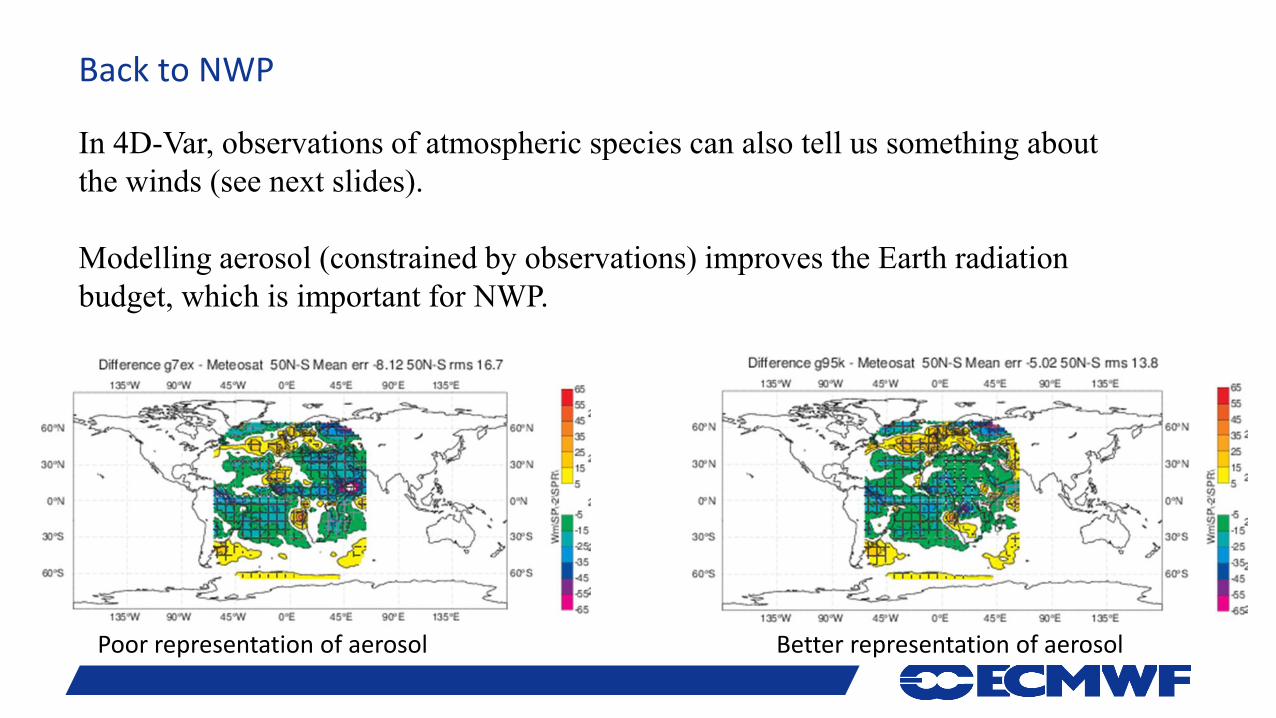
Back to NWP
In 4D-Var, observations of atmospheric species can also tell us something about
the winds (see next slides).
Modelling aerosol (constrained by observations) improves the Earth radiation
budget, which is important for NWP.
Poor representation of aerosol Better representation of aerosol
Slide 46
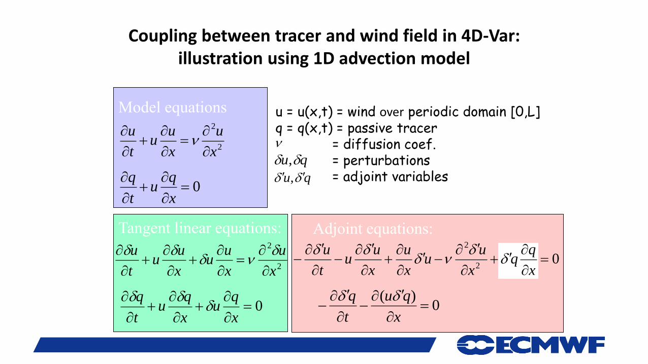
Coupling between tracer and wind field in 4D-Var:illustration using 1D advection model
2
2
x
u
x
uu
t
u
0
x
qu
t
q
2
2
x
u
x
uu
x
uu
t
u
0
x
qu
x
qu
t
q
0
)(
x
qu
t
q
Tangent linear equations: Adjoint equations:
Model equations u = u(x,t) = wind over periodic domain [0,L]q = q(x,t) = passive tracer
= diffusion coef.= perturbations= adjoint variablesqu ,
qu ,
02
2
x
x
uu
x
u
x
uu
t
u
Slide 47
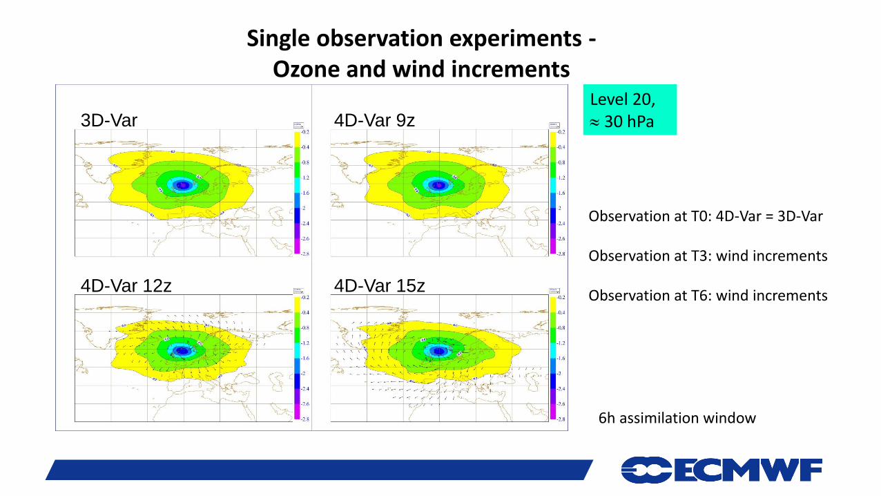
Single observation experiments -Ozone and wind increments
4D-Var 12z 4D-Var 15z
4D-Var 9z3D-Var Level 20, 30 hPa
6h assimilation window
Observation at T0: 4D-Var = 3D-Var
Observation at T3: wind increments
Observation at T6: wind increments
Slide 48
What we have seen today…
Basic theory is the same
For mostly pragmatic reasons we have wound the clock back a bit and make more use of L2 retrievals
Important to correctly use the L2 information (AK, errors, a priori)
Atmospheric composition is much more a boundary value problem than an initial condition problem
Many species and aerosol size distributions make the system very much under-sampled
Progress is made by addressing all areas – still a lot of work to do
Atmospheric composition has the potential to improve various aspects of NWP
Slide 48NWP-SAF Training Course
Recommended