Satellite-based estimation of roughness lengths and displacementheights for wind resource modellingRogier Floors1, Merete Badger1, Ib Troen1, Kenneth Grogan2, and Finn-Hendrik Permien3
1Technical University of Denmark, DTU Wind Energy, Risø Campus, Frederiksborgvej 399, 4000 Roskilde, Denmark2DHI GRAS A/S, Agern Alle 5, 2970 Hørsholm, Denmark3Siemens Gamesa Renewable Energy A/S, Borupvej 16, 7330 Brande, Denmark
Correspondence: Rogier Floors ([email protected])
Abstract. Wind turbines in northern Europe are frequently placed in forests, which sets new wind resource modelling require-
ments. Accurate mapping of the land surface can be challenging at forested sites due to sudden transitions between patches
with very different aerodynamic properties, e.g. tall trees, clearings, and lakes. Tree growth and deforestation can lead to tem-
poral changes of the forest. Global or pan-European land cover data sets fail to resolve these forest properties, aerial lidar
campaigns are costly and infrequent, and hand-digitization is labour-intensive and subjective. Here, we investigate the poten-5
tial of using satellite observations to characterise the land surface in connection with wind energy flow modelling using the
Wind Atlas Analysis and Application Program (WAsP). Collocated maps of the land cover, tree height, and Leaf Area Index
(LAI) have been generated based on observations from the Sentinel-1 and -2 missions combined with the Ice, Cloud, and
Land Elevation Satellite-2 (ICESat-2). Three different forest canopy models are applied to convert these maps to roughness
lengths and displacement heights. We introduce a modified model, which can process detailed land cover maps containing10
both roughness lengths and displacement heights. Extensive validation is carried out through cross-prediction analyses at ten
well-instrumented sites in various landscapes. We demonstrate that using the novel satellite-based input maps leads to lower
cross-prediction errors of the wind power density than land cover databases at a coarser spatial resolution. Differences in the
cross-predictions resulting from the three different canopy models are minor. The satellite-based maps show cross-prediction
errors close to those obtained from aerial lidar scans and hand-digitised maps. This demonstrates the value of using detailed15
satellite-based land cover maps for micro-scale flow modelling.
1 Introduction
Wind turbines on land represent a cost-competitive source of renewable energy (Global Wind Energy Council, 2019). More
than 95% of the global installed wind energy capacity of ≈ 651 GW in 2019 is installed on land (https://www.irena.org/wind).
In the northern Europe’s temperate climates, a vast amount of the land surface is covered by forest. The exploitation of wind20
power within such forests has become more widespread as the hub height of modern wind turbines has exceeded the forest
height (Enevoldsen, 2016).
Wind resource assessment is typically performed with linearized modelling in a wind farm siting tool (e.g. WAsP or Wind-
PRO), which contains several sub-models to predict the flow based on an input wind histogram (Troen and Petersen, 1989).
1
https://doi.org/10.5194/wes-2021-28Preprint. Discussion started: 6 April 2021c© Author(s) 2021. CC BY 4.0 License.

Based on Monin-Obukhov similarity theory (Eq. 1), the flow model can be used to predict the wind speed, U , for any height,25
z above the ground:
U =u∗κ
[lnz− dz0−Ψm
], (1)
where u∗ is the friction velocity, κ is the Von Kármán constant (= 0.4), z0 is the aerodynamic roughness length, and Ψm
represents the stability correction to the profile and depends on z/L, where L is the Monin-Obukhov length (Businger et al.,
1971). At forested sites, the zero-plane displacement height, d is traditionally used in addition to z0 to account for the canopy30
forcing the mean flow to be displaced upwards over forests (Thom, 1971). A dense forest appears more smooth (i.e. a lower
z0) and has a larger d than a sparse forest with clearings and a more in-homogeneous appearance of the same height (Shaw and
Pereira, 1982).
Values of z0 and d can be assessed through manual inspection of the forest at a given site combined with digital maps.
In practice, a background value for z0 and d is set, and adjustments are made for specific areas where the roughness and35
displacement height differ from the background values. Manual assessments are subjective and time-consuming, and they can
lead to a high level of uncertainty of the estimated wind resource (Kelly and Jørgensen, 2017).
Fully automated assessments of z0 and d can be achieved based on global or regional land cover data sets derived from satel-
lite observations. Each land cover class is assigned a value of z0 and d via a land cover table (Jancewicz and Szymanowski,
2017; Floors et al., 2018). State-of-the-art flow modelling tools offer embedded access to such land cover maps and to the40
associated roughness translation tables, which the user may modify. Due to the coarse spatial resolution of global land cover
data sets and the typical minimum-mapping-unit (MMU) of several hectares, the finer-scale variability within a forest, such as
smaller clearings, is not resolved. Further, the available land cover to roughness translation tables may not be fully represen-
tative for the site in question due to the data sets’ global nature. Commonly used tables show very low roughness lengths for
forest land cover classes (Floors et al., 2018; Enevoldsen, 2016).45
Floors et al. (2018) have demonstrated that tree heights and forest densities retrieved from aerial lidar scans can be used to
parameterize z0 and d over the forest. This approach is more physical than the ad-hoc assignment using land cover data sets. It
sets new requirements to the flow modelling tools used for wind energy siting because i) a different type of model is needed to
estimate z0 and d from the tree height and density, and ii) efficient data processing routines are necessary to handle the much
finer resolution of data layers from aerial lidar scans. Several countries in northern Europe have released national aerial lidar50
scans, and dedicated campaigns may be performed in connection with wind farm planning. A limitation of the aerial lidar scans
is each campaign’s high cost and the associated data processing. Therefore, the temporal frequency of such observations is low.
A wealth of new satellite observations with unprecedented spectral properties and spatial and temporal resolutions have
become available, e.g. through Copernicus (https://www.copernicus.eu). Forest monitoring is a key objective of several new
missions because information on deforestation and forest degradation is important in connection with climate change mitiga-55
tion. However, key metrics for wind-resource assessment such as forestry canopy height are still missing or only available at a
low spatial resolution but can be derived through post-processing of the data from available sensors. Here, we hypothesize that
2
https://doi.org/10.5194/wes-2021-28Preprint. Discussion started: 6 April 2021c© Author(s) 2021. CC BY 4.0 License.

these post-processed values of forest canopy height and density retrieved from satellites in a high spatial resolution, can also
be used to estimate wind resources in the same accuracy as aerial lidar scans but at a lower cost.
This paper aims to use tree heights and densities retrieved from satellite observations in connection with flow modelling60
for wind energy. We will map z0 and d from satellite-based forest parameters and use these maps in combination with wind
observations from meteorological masts to predict the wind resource for ten sites worldwide. Wind power densities calculated
using the novel satellite-based data layers will be compared to predictions based on global land cover maps, aerial lidar scans,
and manual digitization for the parameterization of z0 and d.
2 Background65
2.1 Forest parameters from satellites
The Ice, Cloud, and Land Elevation Satellite-2 (ICESat-2) carries the Advanced Topographic Laser Altimeter System (ATLAS),
used to observe the land surface height with great precision. Amongst many other parameters, the mission delivers global forest
canopy heights (Neuenschwander and Pitts, 2019), which are well correlated with canopy heights from aerial lidar scans (Li
et al., 2020) and field measurements (Huang et al., 2019). A mission with similar capabilities to ICESat-2 is the Global70
Ecosystem Dynamics Investigation (GEDI). However GEDI only collects data 52 degrees north and south of the equator,
and therefore does not offer global coverage. Although representing a major advancement in estimating 3D forest structure,
these current spaceborne laser observations are restricted to very narrow footprints, which are insufficient to map wall-to-
wall canopy heights over larger areas. Recent studies have shown that the laser-derived canopy heights can be extrapolated
through different combinations with other satellite observations and machine learning techniques (Csillik et al., 2020; Fagua75
et al., 2019). Typically, the canopy heights from laser measurements are extrapolated using textural information from active
microwave sensors (e.g. Sentinel-1 or ALOS PALSAR) and multispectral information from passive sensors (e.g. Landsat or
Sentinel-2). Li et al. (2020) has pointed out that backscattering coefficients from Sentinel-1 and the variables related to red-edge
bands from Sentinel-2 contribute positively to the prediction of forest canopy heights.
The Leaf Area Index (LAI) is a measure of the one-sided green leaf area per unit ground area in broadleaf canopies and80
as one-half the total needle surface area per unit ground area in coniferous canopies (Chen and Black, 1992). In connection
with flow modelling for wind energy, LAI can be used as a proxy for the forest density (Raupach, 1994). Several space-borne
sensors, operating in the visible and near-infrared range, monitor vegetation properties (including LAI) daily. For example, the
Terra and Aqua satellites each carry a Moderate Resolution Imaging Spectroradiomenter (MODIS). Four-day composites of
LAI are generated routinely from the two instruments in combination. This product has a relatively coarse resolution and a85
pixel size of 500 m. Guzinski and Nieto (2019) has developed a method for downscaling of LAI estimates.
3
https://doi.org/10.5194/wes-2021-28Preprint. Discussion started: 6 April 2021c© Author(s) 2021. CC BY 4.0 License.

2.2 Forest roughness models
Different models can be used to estimate z0 and d from forest canopy heights and densities. Here, we consider the Objective
Roughness Approach (ORA), the Raupach model, and the scalar distribution (SCADIS) model.
2.2.1 The objective roughness approach (ORA)90
The relation between h and z0 and d has been recognized and discussed by many authors (Thom, 1971; De Bruin and Moore,
1985). Because z0 is usually proportional to h, an easy way to obtain z0 and d is by relating them linearly to the canopy height,
z0 = c1h, (2)
and95
d= c2h. (3)
The constant values c1 = 0.1 and c2 = 2/3, were shown in Floors et al. (2018) to yield good results when used for wind energy
flow modelling at a forested site.
2.2.2 The Raupach model
Raupach (1992) developed a model to predict the bulk drag coefficient over a rough surface with a canopy height. The main100
model parameter resulting from his analysis is the frontal area index λ, which for isotropically oriented elements is given by,
λ= 0.5LAI. (4)
To a good approximation, the LAI can be substituted by the canopy area index, which includes the area covered by the canopy
objects that are not leaves (Raupach, 1994). For simplicity, we here refer to the more commonly used LAI throughout the
paper. Raupach (1994) discussed some simplifications to the original model and suggested105
d
h= 1− b, (5)
where
b= 1− exp(−a)a
(6)
and
a=√
2cd1λ. (7)110
cd1 was experimentally found to be equal to 7.5. Finally, the roughness length is estimated as,
z0h
= bexp( −κ
min(√CS +CRλ,cmax)
−Ψh
). (8)
Raupach (1994) suggested the constants to be CS = 0.003, CR = 0.3, cmax = 0.3 and Ψh = 0.193.
4
https://doi.org/10.5194/wes-2021-28Preprint. Discussion started: 6 April 2021c© Author(s) 2021. CC BY 4.0 License.
2.2.3 The SCADIS model
A criticism of the Raupach (1994) model is that some of the constants are highly dependent on the structure of the canopy and115
may not be universally applicable. To address this, one can use a one-dimensional version of a k-ω model, which depends on
the leaf-area density distribution within the canopy. Such an approach was suggested by Sogachev et al. (2002); Sogachev and
Panferov (2006). An additional advantage of this model is that it can estimate z0 and d in non-neutral atmospheric conditions.
The leaf or canopy area density (LAD) profile is frequently described (e.g. Meyers and Tha Paw U, 1986) by a beta proba-
bility density function,120
LAD = LAI
[(z/h
)α−1(1− z/h
)β−1], (9)
where α= 9 and β = 3. The chosen constants are representative of a temperate pine forest. Sogachev et al. (2017) validated
the SCADIS model for flow over a 3D area with forested terrain and found that simulations that explicitly resolve the drag of
the canopy and those that use an effective z0 compare well.
2.3 Model response to LAI125
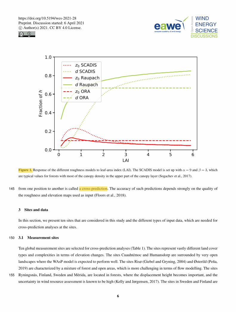
The behaviour of the three forest roughness models for a canopy height h of 10 m as a function of LAI is shown in Fig. 1. The
ORA model does not depend on leaf-area index and is therefore constant, i.e. d/h= 2/3 and z0/h= 0.1. The Raupach and
SCADIS models both show an increasing d as the LAI increases. z0 has the opposite behaviour and decreases to lower values
after an initial maximum of around LAI≈1.
The main differences between the SCADIS and Raupach models occur for a relatively low LAI ∼ 1; using the SCADIS130
model z0/h≈ 0.2 while using the Raupach model z0/h≈ 0.1. The same holds for d, where using the Raupach model yields a
d that is nearly twice that of the SCADIS model. For the more commonly occurring LAI> 3, the differences are minor. When
a different canopy profile is specified, i.e. using α= 5 and β = 3, there are larger differences between the two models.
2.4 Flow modelling and cross-prediction
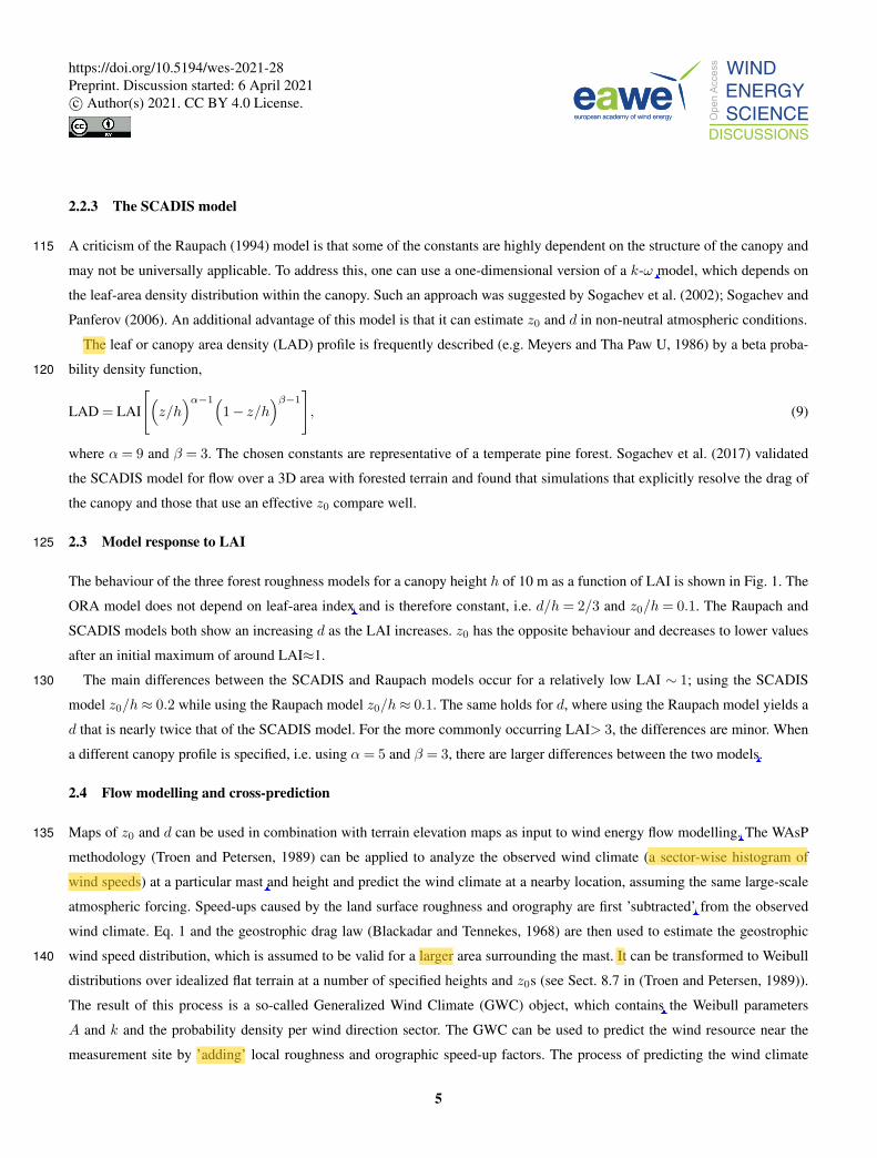
Maps of z0 and d can be used in combination with terrain elevation maps as input to wind energy flow modelling. The WAsP135
methodology (Troen and Petersen, 1989) can be applied to analyze the observed wind climate (a sector-wise histogram of
wind speeds) at a particular mast and height and predict the wind climate at a nearby location, assuming the same large-scale
atmospheric forcing. Speed-ups caused by the land surface roughness and orography are first ’subtracted’ from the observed
wind climate. Eq. 1 and the geostrophic drag law (Blackadar and Tennekes, 1968) are then used to estimate the geostrophic
wind speed distribution, which is assumed to be valid for a larger area surrounding the mast. It can be transformed to Weibull140
distributions over idealized flat terrain at a number of specified heights and z0s (see Sect. 8.7 in (Troen and Petersen, 1989)).
The result of this process is a so-called Generalized Wind Climate (GWC) object, which contains the Weibull parameters
A and k and the probability density per wind direction sector. The GWC can be used to predict the wind resource near the
measurement site by ’adding’ local roughness and orographic speed-up factors. The process of predicting the wind climate
5
https://doi.org/10.5194/wes-2021-28Preprint. Discussion started: 6 April 2021c© Author(s) 2021. CC BY 4.0 License.
0 1 2 3 4 5 6LAI
0.0
0.2
0.4
0.6
0.8
1.0
Frac
tion
of h
z0 SCADISd SCADISz0 Raupachd Raupachz0 ORAd ORA
Figure 1. Response of the different roughness models to leaf-area index (LAI). The SCADIS model is set up with α= 9 and β = 3, which
are typical values for forests with most of the canopy density in the upper part of the canopy layer (Sogachev et al., 2017).
from one position to another is called a cross-prediction. The accuracy of such predictions depends strongly on the quality of145
the roughness and elevation maps used as input (Floors et al., 2018).
3 Sites and data
In this section, we present ten sites that are considered in this study and the different types of input data, which are needed for
cross-prediction analyses at the sites.
3.1 Measurement sites150
Ten global measurement sites are selected for cross-prediction analyses (Table 1). The sites represent vastly different land cover
types and complexities in terms of elevation changes. The sites Cuauhtémoc and Humansdorp are surrounded by very open
landscapes where the WAsP model is expected to perform well. The sites Risø (Giebel and Gryning, 2004) and Østerild (Peña,
2019) are characterized by a mixture of forest and open areas, which is more challenging in terms of flow modelling. The sites
Ryningsnäs, Finland, Sweden and Mérida, are located in forests, where the displacement height becomes important, and the155
uncertainty in wind resource assessment is known to be high (Kelly and Jørgensen, 2017). The sites in Sweden and Finland are
6
https://doi.org/10.5194/wes-2021-28Preprint. Discussion started: 6 April 2021c© Author(s) 2021. CC BY 4.0 License.

from confidential projects, and the exact locations of these can therefore not be disclosed. Perdigao and Alaiz are complex sites
inmountainous terrain. The ruggedness index (RIX) is often used to characterize the flow modelling complexity. It indicates
the percentage of slopes higher than 30% in a 3.5 km circle around the site. For larger values of this index, WAsP has been
found to become inaccurate (Bowen and Mortensen, 1996). This is probably due to increased form drag on steep slopes, not160
accounted for in the surface roughness. In addition, nearby steep slopes are not well handled in the BZ terrain model in WAsP
(Troen and Hansen, 2015).
3.2 Standard land cover data sets
Four course-resolution land cover databases that are regularly applied for wind energy modelling are used in connection with
this analysis (see Table 3).165
The Global Land Cover Characterization (GLCC) dataset provides a coarse 1000 m resolution land cover data set. It is de-
rived from the Advanced Very High Resolution Radiometer (AVHRR) data collected between April 1992 and March 1993. The
AVHHR is a space-borne sensor mounted on a polar-orbiting satellite from the National Oceanic and Atmospheric Administra-
tion (NOAA). The MODIS (MCD12Q1 V6) product provides yearly global land cover between 2001 and 2018 and is derived
from six different classification schemes. It is made using supervised classifications of MODIS Terra and Aqua reflectance170
data. Prior knowledge and ancillary information is used to refine the classifications further. This product has a resolution of
≈ 500 m. The C3S Global Land Cover product provides global coverage at a resolution of 0.002778◦(≈ 300 m). It is consistent
with the global annual land cover series from 1992 to 2015 produced by the European Space Agency (ESA) Climate Change
Initiative (CCI). Version 2.1.1 created from data from 2018 is used here, which has 38 land cover classes. The most recent
version (2018) of the Corine Land Cover (CL2018) inventory is used to analyse sites in Europe. Its minimum mapping unit is175
25 ha, corresponding to a grid resolution of 100 m, and the product has 44 land cover classes.
The coarse-resolution land cover data sets come with standard roughness conversion tables (Table A1–A5, Thøgersen
(2021)). The z0 for forest classes tends to be too low for temperate forests (Floors et al., 2018). Recent studies of Dörenkämper
et al. (2020) and Badger et al. (2015) have highlighted this aspect and have suggested higher z0 for forested areas. To reflect
the uncertainty of z0 assignments, we include these in Table A3–A5. In connection with the C3S Global Land Cover product,180
the z0 classification is based on the data set of 2009 and some of the 23 land cover classes have been split into sub-classes since
then. Therefore, z0 of each subclass is assumed to be identical to z0 of the class it inherits from (see Table A3).
3.3 Novel Sentinel data sets
High-resolution satellite-based data packages have been developed for an area of 40× 40 km around each of the ten sites
described above. Each data package has a regular grid spacing of 20 m by 20 m and includes 1) land cover classification,185
2) LAI, and 3) forest canopy height. The primary data source used for the production of these layers is Copernicus satellite
imagery from the Sentinel-1 and Sentinel-2 missions. Sentinel-1 is a c-band (5.6 cm) Synthetic Aperture Radar sensor, while
Sentinel-2 is an optical sensor providing data in the visible, near-infrared, and shortwave infrared parts of the spectrum. The
land cover classification is based on five land cover classes most relevant for wind modelling (see Table A5). For each site,
7
https://doi.org/10.5194/wes-2021-28Preprint. Discussion started: 6 April 2021c© Author(s) 2021. CC BY 4.0 License.

Table 1. Sites and masts used for cross-prediction analyses. The characteristic land cover and terrain complexity (RIX) are indicated. The
EPSG code identifies the coordinate reference system, including the map projection, datum and zone number (see text) and the x, y and z
columns identify the positions in projected map coordinates.
Site Mast Land cover type RIX (%) EPSG code x (m) y (m) z (m)
Alaiz (ES) 1 Complex 9.5 32630 617609 4731301 20.0, 40.0, 60.0, 80.0
Alaiz (ES) 2 Complex 8.0 32630 617650 4732567 20.0, 40.0, 60.0, 80.0
Cuauhtémoc (MX) Open 0.0 32613 309873 3211836 20.0, 40.0, 60.0, 80.0
Finland (FI) 1 Forest 0.0 32635 60.0, 90.0, 116.5
Finland (FI) 2 Forest 0.0 32635 61.0, 91.0, 116.5
Finland (FI) 3 Forest 0.0 32635 61.0, 91.0, 116.5
Humansdorp (SA) Open 0.0 32735 270726 6222861 20.2, 37.3, 61.1, 62.0
Mérida (MX) Forest 0.0 32616 210700 2339899 20.0, 40.0, 60.0, 80.0
Perdigão (PT) 1 Complex 17.2 32629 607386 4396302 30.0, 60.0
Perdigão (PT) 2 Complex 15.5 32629 607695 4395878 28.0, 57.0, 100.0
Perdigão (PT) 3 Complex 15.6 32629 607874 4395628 30.0, 60.0
Perdigão (PT) 4 Complex 18.1 32629 607877 4396972 60.0
Perdigão (PT) 5 Complex 16.5 32629 607934 4396109 30.0, 60.0
Perdigão (PT) 6 Complex 16.6 32629 608239 4397251 30.0, 60.0
Perdigão (PT) 7 Complex 15.3 32629 608449 4396471 30.0, 60.0, 100.0
Perdigão (PT) 8 Complex 15.7 32629 608628 4396602 30.0, 60.0
Perdigão (PT) 9 Complex 15.5 32629 608827 4396741 30.0, 60.0, 100.0
Risø (DK) Mixed 0.2 32632 694096 6176367 44.2, 76.6, 94.0, 118.0, 125.2
Ryningsnäs (SE) Forest 0.0 32633 559487 6348565 40.0, 59.0, 80.0, 98.0, 120.0, 138.0
Sweden (SE) 1 Forest 0.1 32633 57.8, 80.7, 96.4, 100.7
Sweden (SE) 2 Forest 0.2 32633 31.5, 44.5, 57.0, 59.0
Sweden (SE) 3 Forest 0.3 32633 57.8, 80.9, 96.4, 100.8
Sweden (SE) 4 Forest 0.0 32633 57.7, 80.8, 96.4, 100.8
Sweden (SE) 5 Forest 0.1 32633 32.1, 44.0, 57.3, 59.0
Sweden (SE) 6 Forest 0.3 32633 57.6, 96.4, 100.8
Sweden (SE) 7 Forest 0.2 32633 57.8, 80.9, 96.4, 100.8
Østerild (DK) 1 Mixed 0.1 32632 492766 6327084 40.0, 70.0, 106.0, 140.0, 178.0
Østerild (DK) 2 Mixed 0.0 32632 492767 6322834 40.0, 70.0, 106.0, 140.0, 178.0
8
https://doi.org/10.5194/wes-2021-28Preprint. Discussion started: 6 April 2021c© Author(s) 2021. CC BY 4.0 License.
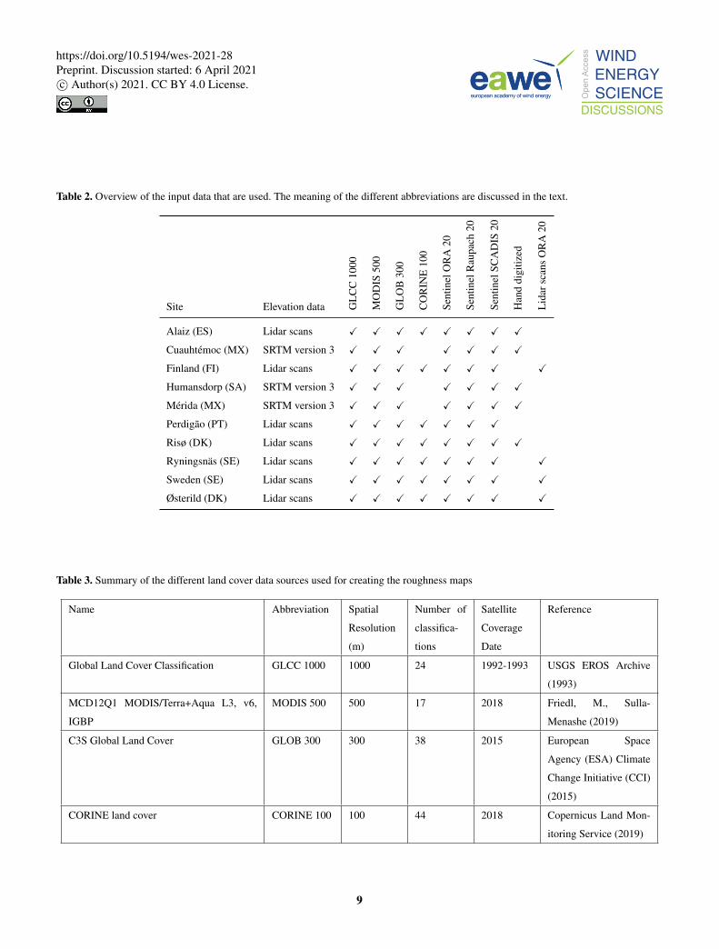
Table 2. Overview of the input data that are used. The meaning of the different abbreviations are discussed in the text.
Site Elevation data GL
CC
1000
MO
DIS
500
GL
OB
300
CO
RIN
E10
0
Sent
inel
OR
A20
Sent
inel
Rau
pach
20
Sent
inel
SCA
DIS
20
Han
ddi
gitiz
ed
Lid
arsc
ans
OR
A20
Alaiz (ES) Lidar scans X X X X X X X XCuauhtémoc (MX) SRTM version 3 X X X X X X XFinland (FI) Lidar scans X X X X X X X XHumansdorp (SA) SRTM version 3 X X X X X X XMérida (MX) SRTM version 3 X X X X X X XPerdigão (PT) Lidar scans X X X X X X XRisø (DK) Lidar scans X X X X X X X XRyningsnäs (SE) Lidar scans X X X X X X X XSweden (SE) Lidar scans X X X X X X X XØsterild (DK) Lidar scans X X X X X X X X
Table 3. Summary of the different land cover data sources used for creating the roughness maps
Name Abbreviation Spatial
Resolution
(m)
Number of
classifica-
tions
Satellite
Coverage
Date
Reference
Global Land Cover Classification GLCC 1000 1000 24 1992-1993 USGS EROS Archive
(1993)
MCD12Q1 MODIS/Terra+Aqua L3, v6,
IGBP
MODIS 500 500 17 2018 Friedl, M., Sulla-
Menashe (2019)
C3S Global Land Cover GLOB 300 300 38 2015 European Space
Agency (ESA) Climate
Change Initiative (CCI)
(2015)
CORINE land cover CORINE 100 100 44 2018 Copernicus Land Mon-
itoring Service (2019)
9
https://doi.org/10.5194/wes-2021-28Preprint. Discussion started: 6 April 2021c© Author(s) 2021. CC BY 4.0 License.

training data have been collected for all land cover classes and used as a dependent variable in a Random Forest machine190
learning model to predict land cover for each 20 x 20 m grid cell. Independent variables used for the land cover classification
model include observations from the Sentinel-1 and Sentinel-2 sensors. LAI has been estimated for all grid cells identified as
forest in the land cover classification through down-scaling of coarse resolution LAI from the MODIS sensor to the 20×20 m
grid of the Sentinel-2 observations (Guzinski and Nieto, 2019).
Forest canopy heights have been estimated for all grid cells identified as forest in the land cover classification. Canopy195
height estimates from the ICESat-2 sensor are used as a dependent variable to train a Support Vector Regression model to
predict forest canopy height for each 20 x 20 m grid cell. Observations from Sentinel-1 and Sentinel-2 are used as independent
variables in the regression model. ICESat-2 provides a globally available dataset from the US National Aeronautics and Space
Administration (NASA) that uses space-borne Lidar technology to estimate ground and vegetation heights. It does this with
six laser beams, scanning a swath of terrain 9 km wide, with each beam having a footprint of 17 m diameter. Because of the200
Sentinel sensors’ importance for obtaining the three layers described above, they are labelled ’Sentinel’ throughout the rest of
this paper.
3.4 Other land cover data sets
For an experienced wind resource engineer, the most accurate way to obtain a land cover dataset is by digitizing the land cover
areas with the biggest impact on the flow and assign a representative z0 to each area. ’Hand-digitized’ maps were made with205
this procedure at Alaiz, Cuauhtémoc, Humansdorp, Merida and Risø (see Table 2). Another approach to obtain an accurate
land cover map is by using lidar scans to estimate h and applying the ORA approach (see Sect. 2.2.1). The cloud point data are
described in the next section, and after obtaining h, the procedure described in Sect. 3.2.1 in Floors et al. (2018) was used to
estimate z0 and d at Ryningsnäs, Sweden and Østerild. These maps are denoted as ’Lidar scans ORA 20’ throughout the rest
of the paper (see Table 2).210
3.5 Elevation data
Elevation data from aerial lidar scans are available for seven of the ten sites analysed here (Table 2). The lidar scans can be
used to retrieve the terrain elevation and estimate the canopy height at forested sites (Popescu et al., 2003; Floors et al., 2018).
The Swedish sites are covered by a national laser campaign conducted in 2013 (Lantmäteriet, 2016). The retrieved elevation
data is available with a resolution of 0.5 first reflections m2m−2 and 20 m x 20 m grid spacing. Further details about the data set215
are given in (Floors et al., 2018). The Finland elevation model is a digital terrain model produced by the National Land Survey
of Finland (Maanmittauslaitos, MML) available at a 10 m x 10 m grid. At the Danish site Østerild, lidar scans are available
with a resolution of 0.5 first reflections m2m−2 whereas for Risø, elevation data are obtained from the 2.5 m contour lines from
"Danmarks Højdemodel" (Styrelsen for Dataforsyning og Effektivisering, 2016).
The two sites Perdigão and Alaiz are particularly complex with large elevation differences and steep slopes. It is well known220
that the BZ flow model fails in these conditions (Bowen and Mortensen, 1996; Troen and Hansen, 2015). Nonetheless, they
can be used to ensure that the developed model does not deteriorate the results for any sites. Aerial lidar scans have been
10
https://doi.org/10.5194/wes-2021-28Preprint. Discussion started: 6 April 2021c© Author(s) 2021. CC BY 4.0 License.

obtained over Perdigão in 2015 (Fernando et al., 2019) and over Alaiz in 2011–12 (Santos et al., 2020). Elevation data for the
two Mexican sites, Cuauhtémoc and Mérida, and the site in South Africa, Humansdorp, are obtained from the Shuttle Radar
Topography Mission (JPL, 2013) at 90 m resolution.225
3.6 Examples from Ryningsnäs
Fig. 2 illustrates the different z0 representations for a 6× 6 km area around the Ryningsäs mast. The GLCC database has the
coarsest resolution of 1000 m, and therefore, it fails to capture any detail near the mast (a). The whole area is represented
by land cover class 14, i.e. evergreen needle-leaf forest, which corresponds to z0 = 1.5 m (Table A1). Likewise, the MODIS
database at 500 m resolution does not capture any detail within the selected area (b); everything is represented as evergreen230
needle-leaf forest with z0 = 1.0 m (Table A2). Globcover, with a resolution of 300 m, represents most of the land cover around
the site as evergreen needle-leaf forest with z0 = 1.5 m (Table A1), and can just capture some of the lakes and open areas (c).
The Corine land cover database captures more details due to its higher resolution of 100 m (d). Most of the area around the
mast is classified as ’mixed forest’ with z0 = 1.1 m (Table A4). The lakes to the southeast of the masts and the open area to the
west of the masts are captured.235
The Sentinel ORA 20 map (e) shows the result of combining the land cover map with the tree height and LAI layers according
to the procedure presented in Sec. 3.3 and using the h to z0 and d conversion from ORA (Sec. 2.2.1). The Sentinel SCADIS
and Raupach maps look very similar to this and are therefore not shown. It can be seen that the map generally contains a wider
range of z0, ranging from 0.0002 m to over 3 m.
Finally, the z0 map obtained using the ORA approach with h obtained from lidar scans is shown in panel (f). Comparing the240
Sentinel-based tree heights (e) with tree heights derived from aerial lidar scans (f), spatially, the areas with lower and higher
h correspond very well. However, z0 derived from Sentinel is generally lower than from the lidar scans. Because in the ORA
approach, z0 is specified as a fraction of h, this indicates a negative bias in h from the Sentinel maps. To investigate this further,
Fig. 3 shows the distribution of h around the Ryningsnäs mast in the pixels that were classified as forest in the Sentinel maps.
The h distribution from Sentinel has a mode of h≈ 17 m and is much more narrow than that from the lidar scans. The lidar245
scan distribution has the mode at h≈ 20 m. Furthermore the h distribution from Sentinel does not have any h > 23 m, while the
lidar scans have h up to more than 33 m. This phenomenon was not only observed at Ryningsnäs, but also at the sites in Finland
(Culic, 2020). We hypothesize that performing a bias correction on h in the Sentinel maps will lead to better wind resource
predictions. We therefore perform a test where h is increased with 30%, which brings the Sentinel and lidar distributions closer
to each other.250
4 Methodology
The WAsP model is a microscale flow model that is frequently employed for wind resource assessments (Troen and Petersen,
1989). It contains submodels for orography, roughness changes, obstacles and stability effects. In the following, we explain
how the roughness and orographic submodels within WAsP are modified to better utilize the high spatial detail of z0 and d
11
https://doi.org/10.5194/wes-2021-28Preprint. Discussion started: 6 April 2021c© Author(s) 2021. CC BY 4.0 License.

Figure 2. Roughness lengths obtained from a 6×6 km square around the Rynignsnäs site (red point) from GLCC 1000 (a), MODIS 500 (b),
Globcover 300 (c), CORINE 100 (d), Sentinel ORA 20 (e) and Lidar scans ORA (f). The approach to obtain z0 from a land cover class is
described in the text. 12
https://doi.org/10.5194/wes-2021-28Preprint. Discussion started: 6 April 2021c© Author(s) 2021. CC BY 4.0 License.

Figure 3. Distribution of h after binning using a width of 0.5 from the aerial lidar scans and from Sentinel.
obtained from the Sentinel data set. We then describe the cross-prediction method that is applied to test the novel Sentinel data255
sets against more conventional input data for wind energy flow modelling. Ryningsnäs is used as an example throughout this
section to illustrate our approach.
4.1 Model setup
The WAsP model consists of a graphical user interface (GUI) and a core model that is written in the programming language
Fortran. In the following, we refer to the core model code that is directly accessed by using the Python programming language260
as interface. The routines are not yet available in the GUI version of WAsP but a version that has them integrated is scheduled
for release in mid-2021. One of the main advantages of the WAsP core model is its speed: to calculate the AEP of a wind farm
typically takes seconds. The newly implemented routines are parallelized using OpenMP in the Fortran language. Because in
the WAsP core each grid point is independently calculated, the problem is easily distributed across central processing units,
CPU’s. To give an impression of this, the grids presented in this section consisting of 22500 points (a 6x6 km area with a265
resolution of 40 m) using the highest resolution maps (and thus the slowest to process), can still be calculated in less than 30
minutes on 1 node with 36 processors of DTU’s supercomputer. The standard settings of the WAsP core model (corresponding
to WAsP GUI version 12.6) are used here unless otherwise specified. In the following, we describe the modifications to the
roughness and orographic submodules. The different parts of the model chain described in this section are shown in Fig. 4.
4.1.1 Forest sub-model270
The ORA and Raupach models are used to obtain z0 and d and were implemented as described in 2.2. The SCADIS model is
run without Coriolis force, because we want to obtain z0 and d for the logarithmic wind profile in the surface layer. The height
of the model domain is specified as 4h. The height of the first model level is specified to be z1 = 0.5z0b, where the background
roughness length z0b = 0.3 m. The SCADIS model is run from an initial logarithmic profile (z0 = z0b) with a wind speed of 10
13
https://doi.org/10.5194/wes-2021-28Preprint. Discussion started: 6 April 2021c© Author(s) 2021. CC BY 4.0 License.

Landcover raster map
Land cover table forforest class
Landcover vectormap
Spider gridanalysis
Raupach(h,LAI)ORA (h) SCADIS
(h,LAI)
Orographicmodel
Elevation vector map
Elevation zoominggrid d zooming grid
Roughnesschange model
z0 zooming grid
Reduced z0 rose
z0 reduction
Geostrophic draglaw
transformation
Sectorwise z0G
Sectorwise d
G
Orographicspeedups
Roughnessspeedups
d reduction
h raster map LAI raster map
Land cover table
h (+LAI) table
Figure 4. Process diagram of the sub-models in WAsP. The rounded rectangles denote data structures and the square boxes denote a method.
m s−1 at the domain top. The time step in the model is set to 300 s. The model integration is terminated when the wind speed at275
the canopy top changes less than 0.001 m s−1 . Finally, z0 and d are then found by fitting dUdz = u∗
κ(z−D) to U and u∗ obtained
in the range from 1.5h to 2.5h.
4.1.2 Roughness sub-model
Previous versions of WAsP use an algorithm, which finds all z0 crossings between the roughness lines defined in a map and
a number of rays extending from the point of interest. In this study we are not only interested in z0 of a land cover patch, but280
we also want to take into account the effect of a displacement height, d. This information has to be passed from the land cover
contour lines to the roughness model. The roughness submodel in WAsP uses vector lines as input and therefore, the satellite
based raster-maps of land cover are converted to a vector-map format.
14
https://doi.org/10.5194/wes-2021-28Preprint. Discussion started: 6 April 2021c© Author(s) 2021. CC BY 4.0 License.

Instead of each line in the map containing a left- and right z0, the new routines expect the input of ’identifier’ lines, i.e. each
line contains an identifier (ID), which represents a certain land cover left and right of the line. This ID is then represented in285
a land cover table, which prescribes the corresponding z0, d and a description of that land cover class (see e.g. Tables A4).
Keeping the land cover table separate from the map has several advantages, like the possibility to perform sensitivity studies
with respect to z0 and d, which has been difficult so far because one has to modify the contour map itself in an external program.
Using the approach above we can process the standard land cover maps (see Section 3.2). The Sentinel maps contain addi-
tional layers with h and LAI. h is discretized into bins of 5 m and the LAI into bins of 1. The result is a Sentinel land cover290
raster map which typically contains 10–40 different classes of forest types plus the classes specified in Table A5.
For the forest class the center of the h and LAI bins are used to estimate z0 and d according to the three roughness models
described in Section 2.2. Because the routines described in Sect 4.1.1 operate on a table and not on the contour lines in the map
itself, the conversion of h and LAI to z0 and d is fast (i.e. the speed of the computation scales with the number of entries in the
land cover table).295
A new routine, here referred to as a spider grid analysis, is developed to process land cover maps. It uses a polar zooming
grid, similarly to the orographic flow model (Troen, 1990). The distance to the first radial segment r0 in the zooming grid is
defined by the user (default r0 = 25 m) and each next segment has a grid spacing that is 5% larger than the previous one. The
number of azimuthal bins (i.e. wind direction sectors) can also be specified by the user and by default is set to 12, i.e. using a
sector width of 30◦. The first sector is always centered at the north.300
For each cell in the zooming grid, the fraction of the total area fi that each of a total of N land cover types in the land cover
table occupies is determined and the roughness length is calculated,
lnz0 =N∑
i=1
fi lnz0i (10)
The displacement height is taken into account similarly to z0 and is calculated for each cell in the zooming grid as
d=N∑
i=1
fidi. (11)305
The zooming-grid analysis of d and z0 from the Sentinel ORA 20 map over Ryningsnäs is shown in Fig. 5a and 5b, respec-
tively. For comparison with Fig. 2, we focus on a circle with a radius of 3 km. It can be seen that for the 0◦sector for an area
up to 2 km away from the mast d≈ 10 and z0 ≈ 2 m, while for the 150◦sector at around 2 km distance there is a lake that
causes lower z0. Another detail visible from close inspection of Fig. 5a, is the very low values of d and z0 in the 150◦sector at
distances less than 100 m away from the mast. This is because of a clearing in the forest in that direction, which has important310
implications for the flow modelling at Ryningsäs, as will be further discussed in Sect. 5.2. We note that Ryningsnäs was also
was extensively investigated by Bergström et al. (2013), who fitted a logarithmic wind profile to the measurements to obtain z0
and d. For the 150◦sector, d was close to zero due to the clearing, while z0 ≈ 2 m.
Fig. 5c shows a so-called reduced roughness rose, which shows the most significant z0 changes in all directions for the
same area as the zooming grid analysis. This roughness rose captures the main features of the area around the site, but it also315
15
https://doi.org/10.5194/wes-2021-28Preprint. Discussion started: 6 April 2021c© Author(s) 2021. CC BY 4.0 License.

a)0
30
60
90
120
150
180
210
240
270
300
330
0
1000
2000
3000
Wind direction (o)
Dis
tanc
e fr
om o
ri. (
m)
0.0
2.5
5.0
7.5
10.0
12.5
d (m)
b)0
30
60
90
120
150
180
210
240
270
300
330
0
1000
2000
3000
Wind direction (o)
Dis
tanc
e fr
om o
ri. (
m)
0.01
0.50
1.00
2.00
z0 (m)
c)0
30
60
90
120
150
180
210
240
270
300
330
0
1000
2000
3000
Wind direction (o)
Dis
tanc
e fr
om o
ri. (
m)
0.01
0.50
1.00
2.00
z0 (m)
Figure 5. Example of a zooming grid analysis of the displacement (a) the roughness length (b) at the Ryningsnäs site up to 3 km distance
and the corresponding reduced z0 rose (c) after finding the most significant z0 changes.
misses some features that perhaps would have been identified ’by eye’. The large amount of clearings and forest patches in all
directions clearly makes it challenging to find the most significant z0 changes.
Because the effect of a roughness change on the wind speed at a certain point is distance dependent, with nearby areas having
a higher impact, the z0 of each area is multiplied with an exponential weighting function as described in Floors et al. (2018).
From these weighted values z0w, the ones that explain most of the variance are stored for further processing (up to maximum of320
nmax). This is done for computational efficiency, so that equations that take into account the effect of internal boundary layers
can be used. These equations are given in Sect. 8.3 in (Troen and Petersen, 1989). The output of these equations are sector-wise
16
https://doi.org/10.5194/wes-2021-28Preprint. Discussion started: 6 April 2021c© Author(s) 2021. CC BY 4.0 License.

speed-up factors, which are used to ’clean’ the wind observations made at a certain point from microscale effects. Apart from
the speed-up factors, z0w is also used to compute a geostrophic (sometimes referred to as an effective or mesoscale) roughness
length z0G.325
Similarly to z0, also d has to be filtered to use it in Eq. 1 and the geostrophic drag law. Therefore, a triangular weighting
function is applied to the zooming d-grid. The average dG in each sector is found by taking the triangular weighted average
up to a distance xd = 10d0, with d0 defined as d at the first cell in the zooming grid at a distance x0 from the origin. The
triangular weight w is 1 at x0 and w = 0 when x > xd. Physically the reason for applying this filter is that it takes some time
for a new logarithmic profile to develop. Thus, taller trees will need longer upstream support to lead to an effective dG that is330
applied in Eq. 1. The sector-wise z0G and dG can finally be used in connection with Eq. 1 and the geostrophic drag law to find
a geostrophic wind climate from an input histogram. This procedure is unaltered from the description in Chapter 8.7 in Troen
and Petersen (1989) and is therefore not further described.
4.1.3 Orographic submodel
The submodule for orography computes speed-ups due to elevation, and WAsP uses the Bessel-expansion on a zooming grid335
(BZ) model (Troen, 1990). The input of the orographic model is a map with elevation lines, which are processed into a polar
zooming grid, with the highest resolution at the center point of the grid. The resolution of the zooming grid depends on the
radius R large enough that the entire map of height contours is contained inside the circle with radius R. Contour lines that are
more than 20 km away from the site are ignored.
Here we are interested in the effects of z0 on the flow modelling and therefore the highest quality terrain elevation map is340
chosen for each of the 10 sites (see Sect. 3.1). We then study the impact of varying the land cover maps only, while keeping
the elevation map constant.
The resulting zooming grid of d obtained by using Eq. 11 is added to the terrain elevation zooming grid. Using this grid,
the methodology described in Troen (1990) is used to calculate wind speed independent, sector-wise orographic speed-ups.
Similarly to the roughness speed-ups, these are used as local perturbations to the flow, which can be used to obtain a wind345
climate that is representative for a large area. In a forest, the introduction of a displacement height can still cause orographic
speed-ups to be different between the Sentinel maps, although the input elevation data are the same.
4.2 Cross-prediction analyses
To identify the best possible baseline for flow modelling using conventional land cover data bases (see Sec. 3.2) as input, we
first perform cross-predictions using the land cover databases in combination with default land cover tables, which come with350
each land cover data set. We then repeat the analyses using the revised tables suggested by Dörenkämper et al. (2020) and
Badger et al. (2015) (Appendix A). Next, the cross-predictions are performed using all other available data sets (see Table 2).
At some sites, there are multiple masts measuring at the same time (see Table 1) and the wind climate from one mast
is used to predict the wind resource at the neighbouring mast. At other sites, only one mast is available and only vertical
cross-predictions are possible, i.e. predictions of the wind distribution from one height to the next at the same mast. Only355
17
https://doi.org/10.5194/wes-2021-28Preprint. Discussion started: 6 April 2021c© Author(s) 2021. CC BY 4.0 License.

measurements between 20 and 200 m are used to avoid using data measured within the roughness sublayer, where the WAsP
model does not apply. In total, there are 1538 possible cross-predictions for evaluation of the different roughness maps.
Observed wind climates are generated for each height and mast from the 10–min. time series of wind speed U and wind
direction θ, which are discretizised into histograms using a bin width of 1 m s−1 and 30 ◦, respectively.
The power per unit area swept by wind turbine blades, P (also referred to as the power density), is given by360
P = 0.5ρU3, (12)
where ρ is the air density. In WAsP the wind distribution is described by sector-wise Weibull distributions and therefore we
can conveniently find P from the Weibull parameters A and k for Nd sectors as
P = ρ
Nd∑
i=1
φiA3iΓ(1 + 3/ki) (13)
where φ is the sector-frequency and ρ is calculated according to the methods described in Floors and Nielsen (2019). Through-365
out this paper we choose to evaluate relative errors of power density,
εP = 100(Pmod
Pobs− 1)
(14)
where P is obtained from the modelled (mod) or observed (obs) Weibull distributions. The statistics reported throughout the
rest of the paper are the bias, εP , and the root-mean-square error (RMSE),√ε2P , where the overbar denotes a mean. We also
include relative errors in wind speed U , which we obtain as described above but instead of Eq. 13, U is computed from the370
Weibull distributions as,
U =Nd∑
i=1
φiAiΓ(1 + 1/ki) (15)
As an example, we use the observed wind speed histogram at the Ryningsnäs mast at 80 m and predict the wind resource at
80 m in the same 6x6 km area as in the previous section, using a raster with a resolution of 40 m.
In Fig. 6a, the elevation is shown; the elevation changes are modest, but there is a hill to the west. In Fig. 6b, the displacement375
height in each point is shown. For clarity, we only focus on d for the most frequently observed westerly sector. In the center of
the map the clearing southeast of the mast position is visible, resulting in lower displacement heights. In addition, displacement
heights of more than 10 m are visible further from the mast to the east and southeast.
The result of combined elevation, displacement and roughness description on the emergent power density in the area is
shown in Fig. 6c. The emergent power density is calculated from the frequency weighted sector-wise A and k parameters in380
each point (Eq. 13). The higher power density due to the flow speed-ups over the hill in the west are clearly visible. Because the
changes in power density due to the introduction of a displacement height are difficult to discern, Fig 6d shows the difference
in percent between P with and without using a displacement height. Using d causes a decrease in power density between 0 and
12%. The area with highest reduction in power density in the center indeed corresponds closely to the area with the highest
displacement heights in Fig 6b.385
18
https://doi.org/10.5194/wes-2021-28Preprint. Discussion started: 6 April 2021c© Author(s) 2021. CC BY 4.0 License.

Figure 6. Map with the terrain elevation (a), the displacement height (b), the power density (c) and the relative difference in power density
compared to a terrain map where d= 0 (d) at Ryningsnäs for westerly winds.
19
https://doi.org/10.5194/wes-2021-28Preprint. Discussion started: 6 April 2021c© Author(s) 2021. CC BY 4.0 License.

5 Results
In the following, we show results of the cross-predictions. We first examine the results per site and then we aggregate results
for all the 10 sites investigated. Because the WAsP model is known to perform poorly in complex terrain with steep slopes,
we exclude sites with a RIX-number higher than 1% in the aggregation (see Table 1). Applying this filter leaves 1082 cross-
prediction for the GLCC 1000 and GLOB 300 databases (global coverage) and 1034 for the CORINE 100 (only Europe)390
database.
5.1 Cross-predictions at wind energy sites
The RMS of εP per site is shown in Fig. 7. The complexity of the Perdigão and Alaiz sites clearly leads to very large errors,
which highlights that higher fidelity flow models that can deal with flow separation should be used at these sites and they will
not be included for further analysis. Other sites where we find rather large errors include Finland and Ryningsnäs. Both are395
forested sites with complex vegetation patterns. This indicates a need for better flow modelling at such in-homogeneous sites.
Humansdorp and Cuauhtémoc, in contrast, are characterized by a relatively simple terrain, which results in a low RMS of εP .
The cross-predictions performed using the novel Sentinel maps as input mostly lead to lower RMS of εP than those using the
standard land cover databases. The three forest roughness models lead to very similar results at all 10 sites.
If we consider only the cross-predictions for sites where aerial lidar scans are available (i.e. Ryningsnäs, Sweden, Finland,400
and Østerild), we see that the RMSE of εP ≈ 10.3% for the aerial lidar scans (Lidar scans ORA 20) and 11.4% for the Sentinel
ORA 20 maps, respectively. At Ryningsnäs, Finland, and Østerild the aerial lidar scans yield lower RMS of εP than the Sentinel
maps, whereas at the Swedish site results are more comparable. This will be further discussed in Sec. 5.2. When we consider
the sites with hand-digitized maps only (i.e. Humansdorp, Alaiz, Merida, Cuauhtémoc, Risø), the RMS of εP is 23.8% for the
hand-digitized map, 27.1% for the Sentinel ORA 20 map and 31.9% for the GLOB 300 map. Thus, improvements in RMS of405
εP when using Sentinel maps compared to hand-digitized maps cannot not be shown.
5.2 Effect of tree height on cross-predictions
The replacement of h with 1.3h in the ORA 20 roughness model leads to a slightly lower RMS of εP for most of the sites
(Fig. 8). This is due to the higher z0 and d that directly results from the higher h. However, the Ryningsnäs site shows a RMS
of εP that is twice as low compared to simulations using h from the original Sentinel maps. This large improvement in RMSE410
is due to the location of the Ryningsnäs mast very close to the forest edge. For the westerly sector, d is nearly doubled, which
has large implications for the predicted power density (see Fig. 6). This indicates that for masts located very close to forest
edges, sensitivity studies are still required and the Sentinel maps should be carefully validated against measured tree heights.
Multiplying h with 1.3 decreased the RMS of εP of simulations with the Sentinel Raupach and SCADIS maps similarly to the
Sentinel ORA maps and these are therefore not shown.415
20
https://doi.org/10.5194/wes-2021-28Preprint. Discussion started: 6 April 2021c© Author(s) 2021. CC BY 4.0 License.

Figure 7. RMS of εP at all different sites, including those in highly complex terrain.
5.3 Aggregated results of cross-predictions
We can now aggregate results from the cross-predictions for the eight sites with low complexity (RIX<1%) to obtain the
average performance of each set of input data in connection with flow modelling in WAsP.
The RMSE in power density for the cross-predictions using standard land cover databases with original and revised rough-
ness translation tables is shown in Fig. 3. The GLCC 1000 generally leads to the highest errors, both when the original and420
revised land cover tables are used. The lowest RMSE of all is achieved with the GLOB 300 maps in combination with the
revised land cover table. The RMSE is reduced for all land cover databases when the revised land cover tables are used instead
of the original ones.
We can now compare results generated with the standard land cover databases with results generated with the novel Sentinel
data layers as input. Fig 10 shows the prediction errors when the WAsP model is run with six different inputs: the three global425
standard land cover data bases with revised roughness translation tables plus three types of Sentinel maps based on the three
different forest roughness models described in Section 2.2. The CORINE 100 database is not available at all sites and is
therefore not shown. Similar result were obtained when selecting only European sites (not shown).
21
https://doi.org/10.5194/wes-2021-28Preprint. Discussion started: 6 April 2021c© Author(s) 2021. CC BY 4.0 License.

Figure 8. RMS εP at simple sites for the model runs with Sentinel ORA 20 maps (Original) and those where the tree height was increased
with 30% .
All maps that share a more advanced forest model, yield lower RMSE (RMS of εP ≈ 11.7) than the standard land cover
databases. Table 4 shows that also the mean bias is lower in the Sentinel maps than in the standard land cover databases.430
Similarly, the errors in wind speed εU are also smaller for the Sentinel maps model runs. The mean bias in εU becomes slightly
negative, but is generally close to zero for all WAsP model runs.
When running WAsP it is often more instructive to evaluate horizontal cross-predictions, because the roughness rose will then
be different for two points. To investigate this, the data was additionally filtered to include only horizontal cross-predictions.
However, this did not change the large differences in εP and εU between the model simulations based on land cover databases435
and Sentinel maps. Also the effect of measuring height was investigated by only including cross-predictions between 50 and
200 m, but also this did not change the general picture that emerges from Table 4.
6 Discussion
For the first time, forest parameters retrieved from the Sentinel and ICESat-2 satellites have been used for wind energy flow
modelling. Our examples demonstrate that the variability of the land cover within forests (e.g. vegetation with different height440
and density, clearings, lakes) is resolved far better by these novel products than standard land cover products with pan-European
or global coverage. The high level of spatial detail in these satellite-based data layers is almost comparable to products derived
22
https://doi.org/10.5194/wes-2021-28Preprint. Discussion started: 6 April 2021c© Author(s) 2021. CC BY 4.0 License.

Figure 9. RMS error in power density (εP , in %) at the low (< 1%) RIX sites using the original and revised land cover databases (see text
and Tables A4 and A3 in the Appendix). MODIS 500 and GLCC 1000 have only one recommended z0 table and are therefore not shown.
Table 4. Errors when modelling at all sites with low complexity (RIX< 1%)
Roughness map RMS εP (%) Mean bias εP (%) RMS εU (%) Mean bias εU (%)
GLCC 1000 19.1 2.5 6.5 0.3
MODIS 500 19.8 2.7 6.6 0.3
GLOB 300 14.5 1.9 5.1 0.1
Sentinel ORA 20 11.6 0.6 4.6 -0.2
Sentinel Raupach 20 11.7 0.1 4.7 -0.4
Sentinel SCADIS 20 11.7 0.6 4.6 -0.2
23
https://doi.org/10.5194/wes-2021-28Preprint. Discussion started: 6 April 2021c© Author(s) 2021. CC BY 4.0 License.

Figure 10. RMS of εP at all sites with low complexity (RIX< 1%).
from aerial lidar scans. This is promising in connection with wind energy flow modelling because the satellite-based data layers
can be produced for any site in the world and updated frequently. The cost of having the satellite-based forest data layers is far
lower than the price of dedicated airborne lidar campaigns thanks to the open access to satellite data archives by Copernicus445
and NASA.
The observed bias in h in the ICESat-2/Sentinel product compared to the lidar scans at Ryningsnäs may partly be due to
the different sensing and retrieval methods applied and partly due to temporal differences of the two tree height products. For
example, the standard canopy height product from ICESat-2 (ATL08) records heights over a 17× 100 m along-track transect,
giving a mismatch with resolution of the lidar scans. Additionally, the tree-growth in temperate forests can be up to a few450
m per year. Therefore, it is important to use the most updated h parameterization for the modelling of wind resources. Our
cross-prediction analyses reveal that adding 30% to tree heights retrieved from Sentinel can improve the accuracy of wind
power predictions. Further research is needed to fully understand and improve the absolute accuracy of tree heights retrieved
from satellite observations. Likewise, the absolute accuracy of forest densities expressed through the LAI should be thoroughly
tested in future work.455
Our analyses show minor differences in RMSE when cross-predictions are performed using Sentinel vs aerial lidar scans
to estimate d and z0. These findings are promising in the light of the lower cost and the global coverage of the satellite-based
data layers. Cross-predictions performed with a manual assessment of z0 lead to a lower RMSE at 2 of the 5 sites in our cross-
24
https://doi.org/10.5194/wes-2021-28Preprint. Discussion started: 6 April 2021c© Author(s) 2021. CC BY 4.0 License.

predictions than any of the automatic assessments based of satellite observations or aerial lidar scans. However, automated
procedures can speed up wind resource assessments and remove the subjective judgement of a siting engineer.460
Our results based on standard land cover databases improve when the land cover to roughness translation tables are modified
specifically for land cover classes related to forests. For wind energy projects within forests, it is, therefore, advisable to use
the newly recommended translation tables A3 and A4 shown in Appendix A rather than the translation tables readily available
through software tools for flow modelling.
Although the differences between the three forest models are small in this study, we find that the Raupach and Scadis model465
perform slightly better than the ORA model when a higher h is used. This indicates that some improvements can be made by
including LAI. The LAI obtained from the Sentinel maps is based on very coarse resolution input data. Therefore, the SCADIS
forest model is likely too advanced for the data used in this study due to the large uncertainty in the input data and the absence
of any information about the canopy density profile. More detailed studies at a higher number of sites, preferably with observed
h and LAD profiles, are needed to validate this result further.470
Using a higher z0 than derived from the maps presented in this paper generally gives better results for the forested sites.
This is thought to be related to roughness length aggregation, i.e. finding z0 for a larger area that correctly prescribes the
momentum flux in surface-layer similarity in connection with Eq. 1. The simple logarithmic averaging applied in Eq. 10
is known to be flawed in heterogeneous conditions. For example, Taylor (1987) suggested accounting for sub-grid variance
of z0 when calculating an effective roughness length. Vihma and Savijärvi (1991) compared model approaches for several475
landscape configurations in Finland and found that z0eff was always higher than a simple logarithmic average. This was also
confirmed by Hasager and Jensen (1999), who found that the difference between the logarithmic average and z0eff was higher
for landscapes with small patches and with a half-to-half mix of rough and smooth patches. For small patches, one can argue
that the form drag of the forest will always lead to a much higher z0eff than implied through logarithmic averaging. However,
an analysis of the effect of z0 aggregation was not attempted in this study, but it’s impacts are likely large for heterogeneous480
sites like Østerild, Finland and Ryningsnäs. Bottema et al. (1998) reviewed a range of z0 aggregation methods, which could be
investigated in future work.
In this study, cross-prediction is used without any manual interference. For an actual wind energy project, much smaller
errors would be achieved using the WAsP model because the site engineer usually has access to measurements at several
heights, which can be used to fit the model nearly perfectly to the measurements. However, it is still important to create a485
z0 map that is as accurate as possible because also stability can cause notable variations in the wind profile. The effect of
atmospheric stability is beyond the scope of this study, and the default settings in WAsP are used, but it is acknowledged that
there can be deviations at some sites.
We note that wind engineers should be careful when using databases such as SRTM in combination with a displacement
length. Because the SRTM product shows the height of the surface, it includes the tree height. If this is not taken into account,490
the turbine or mast might be placed at too high elevation, and there is a risk of double-counting of the effects of the forest.
25
https://doi.org/10.5194/wes-2021-28Preprint. Discussion started: 6 April 2021c© Author(s) 2021. CC BY 4.0 License.

7 Conclusions
We have tested a novel satellite-based product for land surface parameterization in forested areas and quantified the effect of
using this product for wind resource modelling. The novel satellite-based product is based on observations from Sentinel-1, -2
and ICESat-2 and it contains collocated layers of land cover, tree heights and LAI at a 20-m spatial resolution. These maps are495
converted to maps of roughness lengths and displacement heights using three different forest modules of varying complexity.
The simplest way to convert the tree height to z0 and d is by multiplying with a constant (e.g. 1/10). Secondly, a physically
more advanced approach, which also considers the effect of LAI, is implemented. The third module is a 1D version of the
SCADIS model and it takes the effects of varying LAI and canopy density profiles into account. All three forest modules are
used in the WAsP model, which is frequently used for prediction the wind resources from wind measurements.500
We find that the high complexity of forested landscapes is poorly resolved by global and pan-European land cover databases
such as GLCC, MODIS, CORINE and Globcover. The novel satellite-based product leads to more detailed maps of z0 and d,
which are spatially comparable to aerial lidar scans or hand-digitized maps. The z0 retrieved from satellites has a negative bias
compared to the aerial lidar scans and further research is needed to refine the product.
Cross-predictions have been performed at 10 sites with tall masts to evaluate the effect of using different input data sets in505
connection with flow modeling in WAsP. The novel maps from Sentinel lead to a reduction of the RMS of relative errors in
power density at most sites and on average by ≈ 3% points compared to the best performing roughness map obtained from a
coarse-resolution land cover database. This is even after the roughness lengths for specific land cover categories in the coarse-
resolution products are improved. Differences between the three forest modules are minor, showing that the sensitivity of the
WAsP model to different approaches to obtain z0 and d is low.510
The RMS of relative errors in power density found for the Sentinel maps (11.4%) are comparable to those obtained from
aerial lidar scans (10.3%). This finding is very promising because the novel satellite-based maps of z0 and d can be generated
at a lower cost and a higher temporal resolution than aerial lidar campaigns. Processing of the satellite-based maps is fully
automated. For sites that show a potential for wind power projects, the new routines and products could replace current practices
of land cover analysis, which is time-consuming and plagued by subjective assessments.515
Appendix A
The land cover tables for the land cover databases that were investigated in this paper are supplied in Tables A1-A5. The
references to the land cover databases can be found in Sec. 3.2.
Code and data availability. The numerical results are generated with proprietary software.
26
https://doi.org/10.5194/wes-2021-28Preprint. Discussion started: 6 April 2021c© Author(s) 2021. CC BY 4.0 License.
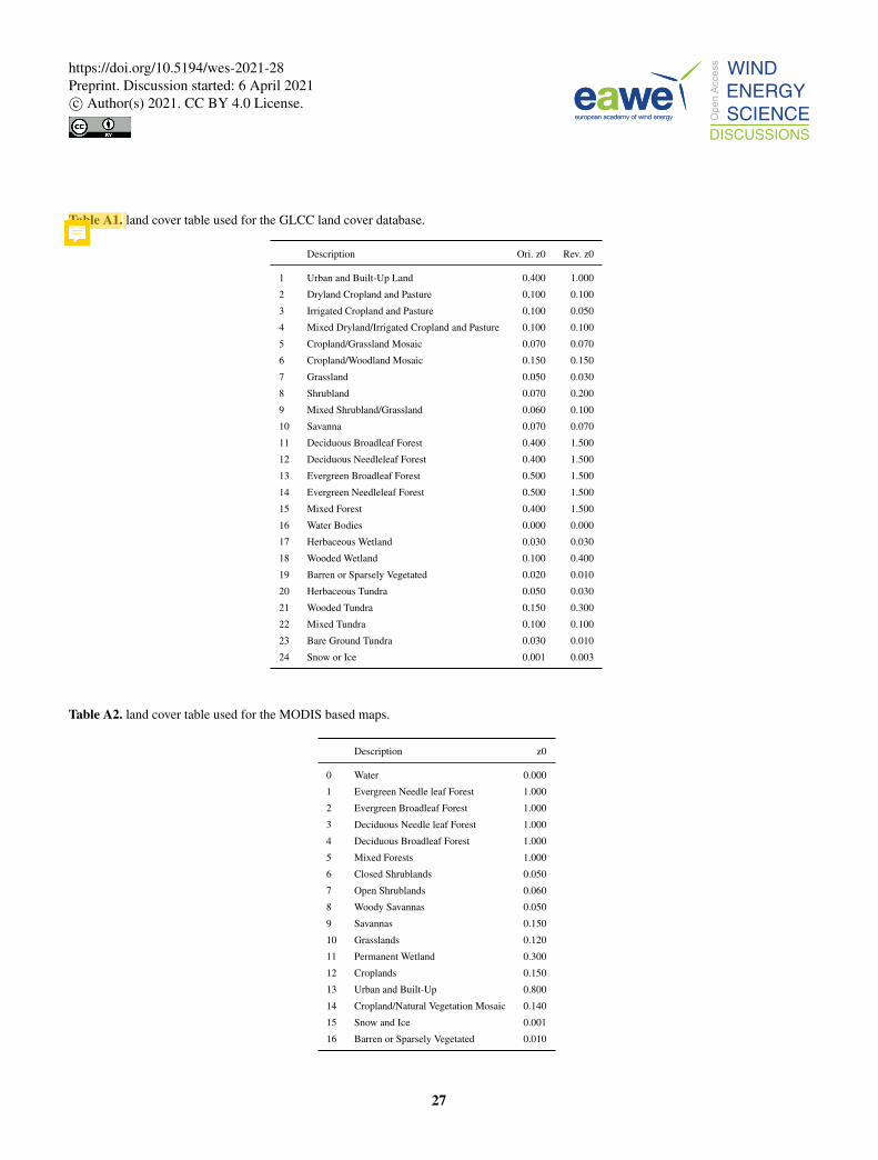
Table A1. land cover table used for the GLCC land cover database.
Description Ori. z0 Rev. z0
1 Urban and Built-Up Land 0.400 1.000
2 Dryland Cropland and Pasture 0.100 0.100
3 Irrigated Cropland and Pasture 0.100 0.050
4 Mixed Dryland/Irrigated Cropland and Pasture 0.100 0.100
5 Cropland/Grassland Mosaic 0.070 0.070
6 Cropland/Woodland Mosaic 0.150 0.150
7 Grassland 0.050 0.030
8 Shrubland 0.070 0.200
9 Mixed Shrubland/Grassland 0.060 0.100
10 Savanna 0.070 0.070
11 Deciduous Broadleaf Forest 0.400 1.500
12 Deciduous Needleleaf Forest 0.400 1.500
13 Evergreen Broadleaf Forest 0.500 1.500
14 Evergreen Needleleaf Forest 0.500 1.500
15 Mixed Forest 0.400 1.500
16 Water Bodies 0.000 0.000
17 Herbaceous Wetland 0.030 0.030
18 Wooded Wetland 0.100 0.400
19 Barren or Sparsely Vegetated 0.020 0.010
20 Herbaceous Tundra 0.050 0.030
21 Wooded Tundra 0.150 0.300
22 Mixed Tundra 0.100 0.100
23 Bare Ground Tundra 0.030 0.010
24 Snow or Ice 0.001 0.003
Table A2. land cover table used for the MODIS based maps.
Description z0
0 Water 0.000
1 Evergreen Needle leaf Forest 1.000
2 Evergreen Broadleaf Forest 1.000
3 Deciduous Needle leaf Forest 1.000
4 Deciduous Broadleaf Forest 1.000
5 Mixed Forests 1.000
6 Closed Shrublands 0.050
7 Open Shrublands 0.060
8 Woody Savannas 0.050
9 Savannas 0.150
10 Grasslands 0.120
11 Permanent Wetland 0.300
12 Croplands 0.150
13 Urban and Built-Up 0.800
14 Cropland/Natural Vegetation Mosaic 0.140
15 Snow and Ice 0.001
16 Barren or Sparsely Vegetated 0.010
27
https://doi.org/10.5194/wes-2021-28Preprint. Discussion started: 6 April 2021c© Author(s) 2021. CC BY 4.0 License.

Table A3. land cover table used for the Globcover/ESA-CCI land cover database.
Description Ori. z0 Rev. z0
0 No data 0.000 0.000
10 Cropland, rainfed 0.100 0.100
11 Cropland rainfed, Herbaceous cover 0.100 0.100
12 Cropland rainfed, Tree or shrub cover 0.200 0.200
20 Cropland, irrigated or post-flooding 0.070 0.050
30 Mosaic cropland (>50%) / natural vegetation (t... 0.070 0.200
40 Mosaic natural vegetation (tree, shrub, herbac... 0.500 0.300
50 Tree cover, broadleaved, evergreen, closed to ... 0.400 1.500
60 Tree cover, broadleaved, deciduous, closed to ... 0.400 1.000
61 Tree cover, broadleaved, deciduous, closed (>40%) 0.400 1.000
62 Tree cover, broadleaved, deciduous, open (15-40%) 0.400 0.800
70 Tree cover, needleleaved, evergreen, closed to... 0.500 1.500
71 Tree cover, needleleaved, evergreen, closed (>... 0.500 1.500
72 Tree cover, needleleaved, evergreen, open (15-... 0.500 1.500
80 Tree cover, needleleaved, deciduous, closed to... 0.500 1.200
81 Tree cover, needleleaved, deciduous, closed (>... 0.500 1.200
82 Tree cover, needleleaved, deciduous, open (15-... 0.500 1.200
90 Tree cover, mixed leaf type (broadleaved and n... 0.400 1.500
100 Mosaic tree and shrub (>50%) / herbaceous cove... 0.400 0.200
110 Mosaic herbaceous cover (>50%) / tree and shru... 0.070 0.100
120 Shrubland 0.070 0.100
121 Shrubland evergreen 0.070 0.200
122 Shrubland deciduous 0.070 0.200
130 Grassland 0.070 0.030
140 Lichens and mosses 0.050 0.010
150 Sparse vegetation (tree, shrub, herbaceous cov... 0.070 0.050
151 Sparse tree (<15%) 0.070 0.050
152 Sparse shrub (<15%) 0.070 0.050
153 Sparse herbaceous cover (<15%) 0.070 0.050
160 Tree cover, flooded, fresh or brakish water 0.100 0.800
170 Tree cover, flooded, saline water 0.100 0.600
180 Shrub or herbaceous cover, flooded, fresh/sali... 0.400 0.100
190 Urban areas 0.400 1.000
200 Bare areas 0.020 0.005
201 Consolidated bare areas 0.020 0.005
202 Unconsolidated bare areas 0.020 0.005
210 Water bodies 0.000 0.000
220 Permanent snow and ice 0.001 0.003
28
https://doi.org/10.5194/wes-2021-28Preprint. Discussion started: 6 April 2021c© Author(s) 2021. CC BY 4.0 License.
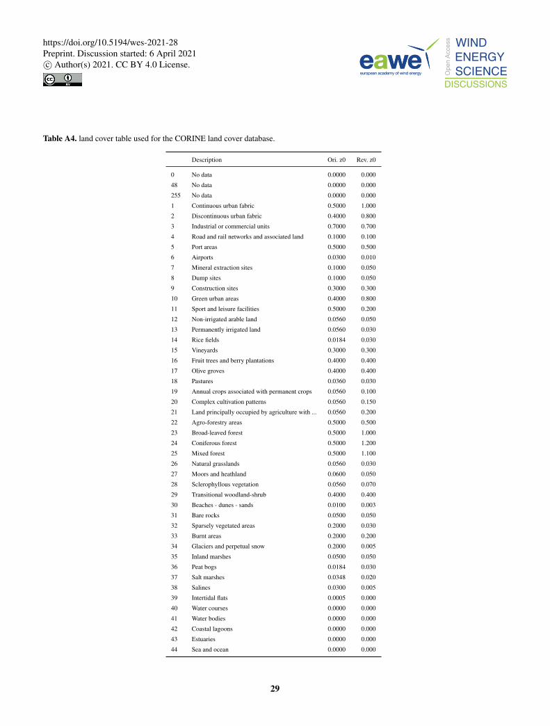
Table A4. land cover table used for the CORINE land cover database.
Description Ori. z0 Rev. z0
0 No data 0.0000 0.000
48 No data 0.0000 0.000
255 No data 0.0000 0.000
1 Continuous urban fabric 0.5000 1.000
2 Discontinuous urban fabric 0.4000 0.800
3 Industrial or commercial units 0.7000 0.700
4 Road and rail networks and associated land 0.1000 0.100
5 Port areas 0.5000 0.500
6 Airports 0.0300 0.010
7 Mineral extraction sites 0.1000 0.050
8 Dump sites 0.1000 0.050
9 Construction sites 0.3000 0.300
10 Green urban areas 0.4000 0.800
11 Sport and leisure facilities 0.5000 0.200
12 Non-irrigated arable land 0.0560 0.050
13 Permanently irrigated land 0.0560 0.030
14 Rice fields 0.0184 0.030
15 Vineyards 0.3000 0.300
16 Fruit trees and berry plantations 0.4000 0.400
17 Olive groves 0.4000 0.400
18 Pastures 0.0360 0.030
19 Annual crops associated with permanent crops 0.0560 0.100
20 Complex cultivation patterns 0.0560 0.150
21 Land principally occupied by agriculture with ... 0.0560 0.200
22 Agro-forestry areas 0.5000 0.500
23 Broad-leaved forest 0.5000 1.000
24 Coniferous forest 0.5000 1.200
25 Mixed forest 0.5000 1.100
26 Natural grasslands 0.0560 0.030
27 Moors and heathland 0.0600 0.050
28 Sclerophyllous vegetation 0.0560 0.070
29 Transitional woodland-shrub 0.4000 0.400
30 Beaches - dunes - sands 0.0100 0.003
31 Bare rocks 0.0500 0.050
32 Sparsely vegetated areas 0.2000 0.030
33 Burnt areas 0.2000 0.200
34 Glaciers and perpetual snow 0.2000 0.005
35 Inland marshes 0.0500 0.050
36 Peat bogs 0.0184 0.030
37 Salt marshes 0.0348 0.020
38 Salines 0.0300 0.005
39 Intertidal flats 0.0005 0.000
40 Water courses 0.0000 0.000
41 Water bodies 0.0000 0.000
42 Coastal lagoons 0.0000 0.000
43 Estuaries 0.0000 0.000
44 Sea and ocean 0.0000 0.000
29
https://doi.org/10.5194/wes-2021-28Preprint. Discussion started: 6 April 2021c© Author(s) 2021. CC BY 4.0 License.

Table A5. land cover table used for the Sentinel based maps.
Description z0
0 Non-forest (cropland, grassland, other) 0.03
1 Forest ORA, Raupach or SCADIS model
2 Water bodies 0.00
3 Urban/Built up 1.00
4 Open forest 0.40
Author contributions. RF generated the results, contributed to the WAsP model code and drafted the manuscript. MB coordinated the work520
and revised the manuscript. IT developed most of the methods and code in the WAsP model and contributed to the preparation of the
manuscript. KG created the Sentinel data layers and wrote a section of the manuscript. FP helped with data-processing and preparation of
the manuscript.
Competing interests. The high-resolution forest data layers generated from Sentinel are sold by DHI GRAS A/S, where KG is employed.
The WAsP software is maintained and sold by DTU Wind Energy, where RF and MB are employed.525
Data availability. Sample data packages containing the Sentinel forest data layers for selected sites are available at https://help.emd.dk/
mediawiki/index.php?title=Innowind_Premium_Data_Layers. The wind measurements from the mast in South Africa (WM08) are available
at http://wasadata.csir.co.za/wasa1/WASAData. Data from the two Mexican masts (M02 and M03) is available at https://aems.ineel.mx/
aemdata/MemberPages/Download.aspx?lang=EN.
Acknowledgements. This work has received funding from the H2020 e-shape project (grant agreement 820852), from Innovation Fund530
Denmark through the InnoWind project (6172-00004B), and from the Ministry of Foreign Affairs of Denmark administered by Danida
Fellowship Centre through the ‘multi-scale and model-chain evaluation of wind atlases’ (MEWA) project (17-M01-DTU). We acknowledge
the providers of global and pan-European land cover data sets: US Geological Survey for GLCC and MODIS, ESA Climate Change Initiative
and in particular its Land Cover project as the source of the CCI-LC database, and ESA Land Monitoring Service for CORINE. ESA and
the European Commission are acknowledged for Copernicus Sentinel data. NASA are acknowledged for ICESat-2 data, and in particular for535
regular consultation through the Early Adopter Program. The Ingeborg and Leo Dannin Prize for Scientific Research (2013) is acknowledged
for the aerial lidar campaign over Perdigão. Ebba Dellwik from DTU is thanked for preparation of aerial lidar data and Andreas Bechmann
for his review of the paper. We acknowledge the Wind Atlas for South Africa project for the wind observations near Humansdorp (CSIR,
2020) and the Mexican Wind Atlas project for observations at the Mexican sites (INEEL, 2020). Technicians of DTU are acknowledged for
the maintenance of the Risø and Østerild masts.540
30
https://doi.org/10.5194/wes-2021-28Preprint. Discussion started: 6 April 2021c© Author(s) 2021. CC BY 4.0 License.

References
Badger, J., Hahmann, A., Larsen, X. G., Badger, M., Kelly, M., Davis, N., Olsen, B. T., and Mortensen, N. G.: The Global Wind
Atlas, Tech. rep., DTU Wind Energy, Roskilde, Denmark, https://www.energiteknologi.dk/sites/energiteknologi.dk/files/slutrapporter/
gwa{_}64011-0347{_}finalreport.pdf, 2015.
Bergström, H. ., Alfredsson, H. ., Arnqvist, J. ., Carlén, I. ., Dellwik, E. ., Fransson, J. ., Ganander, H. ., Mohr, M. ., Segalini, A. ., Söderberg,545
S., Bergström, H., Alfredsson, H., Carlén, J., Dellwik, I., Ganander, J., and Mohr, H.: Wind power in forests: Winds and effects on loads,
Tech. rep., Uppsala University, Stockholm, https://orbit.dtu.dk/en/publications/wind-power-in-forests-winds-and-effects-on-loads, 2013.
Blackadar, A. K. and Tennekes, H.: Asymptotic Similarity in Neutral Barotropic Planetary Boundary Layers, Journal of the
Atmospheric Sciences, 25, 1015–1020, https://doi.org/10.1175/1520-0469(1968)025<1015:ASINBP>2.0.CO;2, http://journals.
ametsoc.org/doi/abs/10.1175/1520-0469(1968)025{%}3C1015:ASINBP{%}3E2.0.CO;2http://journals.ametsoc.org/doi/abs/10.1175/550
1520-0469{%}281968{%}29025{%}3C1015{%}3AASINBP{%}3E2.0.CO{%}3B2, 1968.
Bottema, M., Klaasen, W., and Hopwood, W.: Landscape Roughness Parameters for Sherwood Forest – Validation of Aggregation
Models, Boundary-Layer Meteorol., 89, 317–347, https://doi.org/10.1023/A:1001795509379, https://link.springer.com/article/10.1023/A:
1001795509379, 1998.
Bowen, A. J. and Mortensen, N. G.: Exploring the limits of WAsP the wind atlas analysis and application program, in: Eur. Union Wind555
energy Conf. Proc., edited by A. Zervos, H. Ehmann, P. H., pp. 584–587, H.S. Stephens and Associates, Bedford, https://orbit.dtu.dk/en/
publications/exploring-the-limits-of-wasp-the-wind-atlas-analysis-and-applicat, 1996.
Businger, J. A., Wyngaard, J. C., Izumi, Y., and Bradley, E. F.: Flux-Profile Relationships in the Atmospheric Surface
Layer, J. Atmos. Sci., 28, 181–189, https://doi.org/10.1175/1520-0469(1971)028<0181:FPRITA>2.0.CO;2, http://journals.
ametsoc.org/doi/abs/10.1175/1520-0469(1971)028{%}3C0181:FPRITA{%}3E2.0.CO;2http://journals.ametsoc.org/doi/abs/10.1175/560
1520-0469{%}281971{%}29028{%}3C0181{%}3AFPRITA{%}3E2.0.CO{%}3B2, 1971.
Chen, J. and Black, T.: Defining Leaf-Area Index for non-flat leaves, Plant Cell and Environment, 15, 421–429,
https://doi.org/10.1111/j.1365-3040.1992.tb00992.x, 1992.
Copernicus Land Monitoring Service: CORINE Land Cover 2018, https://land.copernicus.eu/pan-european/corine-land-cover/clc2018,
2019.565
Csillik, O., Kumar, P., and Asner, G. P.: Challenges in estimating tropical forest canopy height from planet dove imagery, Remote Sensing,
12, https://doi.org/10.3390/rs12071160, 2020.
CSIR: WASA measurements, http://wasa.csir.co.za/web/ProjectListText.aspx?{&}Rnd=970089, 2020.
Culic, P.: Enhancing the objective roughness assessment approach with Leaf-Area-Index data for wind turbine siting, Msc thesis, Technical
University of Denmark, 2020.570
De Bruin, H. A. and Moore, C. J.: Zero-plane displacement and roughness length for tall vegetation, derived from a simple mass conserva-
tion hypothesis, Boundary-Layer Meteorology, 31, 39–49, https://doi.org/10.1007/BF00120033, https://link.springer.com/article/10.1007/
BF00120033, 1985.
Dörenkämper, M., Olsen, B. T., Witha, B., Hahmann, A. N., Davis, N. N., Barcons, J., Ezber, Y., García-Bustamante, E., González-Rouco,
J. F., Navarro, J., Sastre-Marugán, M., Sıle, T., Trei, W., Žagar, M., Badger, J., Gottschall, J., Sanz Rodrigo, J., and Mann, J.: The Making575
of the New European Wind Atlas – Part 2: Production and evaluation, Geosci. Model Dev., 13, 5079–5102, https://doi.org/10.5194/gmd-
13-5079-2020, https://gmd.copernicus.org/articles/13/5079/2020/, 2020.
31
https://doi.org/10.5194/wes-2021-28Preprint. Discussion started: 6 April 2021c© Author(s) 2021. CC BY 4.0 License.

Enevoldsen, P.: Onshore wind energy in Northern European forests: Reviewing the risks, https://doi.org/10.1016/j.rser.2016.02.027, 2016.
European Space Agency (ESA) Climate Change Initiative (CCI): Land cover classification gridded maps from 1992 to present derived from
satellite observations, v2.0.7, https://cds.climate.copernicus.eu/cdsapp{#}!/dataset/satellite-land-cover?tab=overview, 2015.580
Fagua, J. C., Jantz, P., Rodriguez-Buritica, S., Duncanson, L., and Goetz, S. J.: Integrating LiDAR, multispectral and SAR data to estimate
and map canopy height in tropical forests, Remote Sensing, 11, https://doi.org/10.3390/rs11222697, 2019.
Fernando, H., Mann, J., Palma, J., Lundquist, J., Barthelmie, R. J., BeloPereira, M., Brown, W., Chow, F., Gerz, T., Hocut, C., Klein, P., Leo,
L., Matos, J., Oncley, S., Pryor, S., Bariteau, L., Bell, T., Bodini, N., Carney, M., Courtney, M., Creegan, E., Dimitrova, R., Gomes, S.,
Hagen, M., Hyde, J., Kigle, S., Krishnamurthy, R., Lopes, J., Mazzaro, L., Neher, J., Menke, R., Murphy, P., Oswald, L., Otarola-Bustos,585
S., Pattantyus, A., Rodrigues, C. V., Schady, A., Sirin, N., Spuler, S., Svensson, E., Tomaszewski, J., Turner, D., van Veen, L., Vasiljevic,
N., Vassallo, D., Voss, S., Wildmann, N., and Wang, Y.: The Perdigão: Peering into Microscale Details of Mountain Winds, Bulletin of
the American Meteorological Society, 100, 799–820, https://doi.org/10.1175/BAMS-D-17-0227.1, 2019.
Floors, R. and Nielsen, M.: Estimating Air Density Using Observations and Re-Analysis Outputs for Wind Energy Purposes, Energies, 12,
2038, https://doi.org/10.3390/en12112038, https://www.mdpi.com/1996-1073/12/11/2038, 2019.590
Floors, R., Enevoldsen, P., Davis, N., Arnqvist, J., and Dellwik, E.: From lidar scans to roughness maps for wind resource modelling
in forested areas, Wind Energy Sci., 3, 353–370, https://doi.org/10.5194/wes-3-353-2018, https://www.wind-energ-sci.net/3/353/2018/,
2018.
Friedl, M., Sulla-Menashe, D.: MCD12Q1 MODIS/Terra+Aqua Land Cover Type Yearly L3 Global 500m SIN Grid V006,
https://doi.org/10.5067/MODIS/MCD12Q1.006, 2019.595
Giebel, G. and Gryning, S.-E.: Shear and stability in high met masts , and how WAsP treats it,
https://www.semanticscholar.org/paper/Shear-and-stability-in-high-met-masts-{%}2C-and-how-it-Giebel-Gryning/
4624ab387a8135a4437aae4dd1df1276b3b4f302{#}citing-papers, 2004.
Global Wind Energy Council: Global Wind Energy Report: Annual Market Update 2019, www.gwec.net, 2019.
Guzinski, R. and Nieto, H.: Evaluating the feasibility of using Sentinel-2 and Sentinel-3 satellites for high-resolution evapotranspiration600
estimations, Remote Sens. Environ., 221, 157–172, https://doi.org/10.1016/j.rse.2018.11.019, 2019.
Hasager, C. B. and Jensen, N. O.: Surface-flux aggregation in heterogeneous terrain, Q. J. R. Meteorol. Soc., 125, 2075–2102,
https://doi.org/10.1002/qj.49712555808, http://doi.wiley.com/10.1002/qj.49712555808, 1999.
Huang, H., Liu, C., and Wang, X.: Constructing a finer-resolution Forest Height in China Using ICESat/GLAS, Landsat and ALOS PALSAR
data and height patterns of natural forests and plantations, Remote Sensing, 11, https://doi.org/10.3390/rs11151740, 2019.605
INEEL: Mexico measurements, http://aems.ineel.mx/, 2020.
Jancewicz, K. and Szymanowski, M.: The Relevance of Surface Roughness Data Qualities in Diagnostic Modeling of Wind Velocity in Com-
plex Terrain: A Case Study from the Snieznik Massif (SW Poland), Pure Appl. Geophys., 174, 569–594, https://doi.org/10.1007/s00024-
016-1297-9, 2017.
JPL, N.: NASA Shuttle Radar Topography Mission Global 3 arc second, https://doi.org/https://doi.org/10.5067/MEaSUREs/SRTM/SRTMGL3N.003,610
https://doi.org/10.5067/MEaSUREs/SRTM/SRTMGL3N.003, 2013.
Kelly, M. and Jørgensen, H. E.: Statistical characterization of roughness uncertainty and impact on wind resource estimation, Wind Energy
Sci., 2, 189–209, https://doi.org/10.5194/wes-2-189-2017, https://www.wind-energ-sci.net/2/189/2017/, 2017.
32
https://doi.org/10.5194/wes-2021-28Preprint. Discussion started: 6 April 2021c© Author(s) 2021. CC BY 4.0 License.

Li, W., Niu, Z., Shang, R., Qin, Y., Wang, L., and Chen, H.: High-resolution mapping of forest canopy height using machine learning
by coupling ICESat-2 LiDAR with Sentinel-1, Sentinel-2 and Landsat-8 data, International Journal of Applied Earth Observation and615
Geoinformation, 92, 102 163, https://doi.org/10.1016/j.jag.2020.102163, 2020.
Meyers, T. and Tha Paw U, K.: Testing of a higher-order closure model for modeling airflow within and above plant canopies, Boundary-
Layer Meteorol., 37, 297–311, https://doi.org/10.1007/BF00122991, http://link.springer.com/10.1007/BF00122991, 1986.
Neuenschwander, A. and Pitts, K.: The ATL08 land and vegetation product for the ICESat-2 Mission, Remote Sensing of Environment, 221,
247–259, https://doi.org/10.1016/j.rse.2018.11.005, 2019.620
Peña, A.: Østerild: A natural laboratory for atmospheric turbulence, J. Renew. Sustain. Energy, 11, 063 302,
https://doi.org/10.1063/1.5121486, http://aip.scitation.org/doi/10.1063/1.5121486, 2019.
Popescu, S. C., Wynne, R. H., and Nelson, R. F.: Estimating plot-level tree heights with lidar: Local filtering with a canopy-height based
variable window size, Computers and Electronics in Agriculture, 37, 71–95, https://doi.org/10.1016/S0168-1699(02)00121-7, 2003.
Raupach, M. R.: Drag and drag partition on rough surfaces, Boundary-Layer Meteorol., 60, 375–395, https://doi.org/10.1007/BF00155203,625
https://link.springer.com/article/10.1007/BF00155203, 1992.
Raupach, M. R.: Simplified expressions for vegetation roughness length and zero-plane displacement as functions of canopy height and area
index, Boundary-Layer Meteorol., 71, 211–216, https://doi.org/10.1007/BF00709229, 1994.
Santos, P., Mann, J., Vasiljevic, N., Cantero, E., Rodrigo, J. S., Borbón, F., Martínez-villagrasa, D., Martí, B., and Cuxart, J.: The Alaiz Ex-
periment : untangling multi-scale stratified flows over complex terrain, Wind Energy Sci. Discuss., pp. 1–24, https://doi.org/10.5194/wes-630
2020-89, 2020.
Shaw, R. H. and Pereira, A. R.: Aerodynamic roughness of a plant canopy: A numerical experiment, Agric. Meteorol., 26, 51–65,
https://doi.org/10.1016/0002-1571(82)90057-7, 1982.
Sogachev, A. and Panferov, O.: Modification of two-equation models to account for plant drag, Boundary-Layer Meteorol., 121, 229–266,
https://doi.org/10.1007/s10546-006-9073-5, 2006.635
Sogachev, A., Menzhulin, G. V., Heimann, M., and Lloyd, J.: A simple three-dimensional canopy – planetary boundary layer simulation
model for scalar concentrations and fluxes, Tellus B Chem. Phys. Meteorol., 54, 784–819, https://doi.org/10.3402/tellusb.v54i5.16729,
2002.
Sogachev, A., Cavar, D., Kelly, M. C., and Bechmann, A.: Effective roughness and displacement height over forested areas, via reduced-
dimension CFD, Tech. rep., DTU, Roskilde, Denmark, 2017.640
Styrelsen for Dataforsyning og Effektivisering: Danmarks Højdemodel , DHM / Terræn, Tech. Rep. August, Styrelsen for Dataforsyning og
Effektivisering, https://download.kortforsyningen.dk/content/dhmh{\T1\o}jdekurver, 2016.
Taylor, P. A.: Comments and further analysis on effective roughness lengths for use in numerical three-dimensional models, Boundary-Layer
Meteorol., 39, 403–418, https://doi.org/10.1007/BF00125144, http://link.springer.com/10.1007/BF00125144, 1987.
Thøgersen, M.: EMD Wiki, https://help.emd.dk/mediawiki/index.php?title=Category{%}3ADigital{_}Roughness{_}Data, 2021.645
Thom, A. S.: Momentum absorption by vegetation, Quarterly Journal of the Royal Meteorological Society, 97, 414–428,
https://doi.org/10.1002/qj.49709741404, http://doi.wiley.com/10.1002/qj.49709741404, 1971.
Troen, I.: A high resolution spectral model for flow in complex terrain, pp. 417–420, American Meteorological Society, Boston, MA, 1990.
Troen, I. and Hansen, B. O.: Wind resource estimation in complex terrain: Prediction skill of linear and nonlinear micro-scale models, in:
AWEA Wind. Conf. Exhib., p. 7, Roskilde, Denmark, 2015.650
Troen, I. and Petersen, E. L.: European Wind Atlas, Risø National Laboratory, Roskilde, Denmark, 1989.
33
https://doi.org/10.5194/wes-2021-28Preprint. Discussion started: 6 April 2021c© Author(s) 2021. CC BY 4.0 License.

USGS EROS Archive: Land Cover Products - Global Land Cover Characterization (GLCC), https://doi.org/10.5066/F7GB230D, 1993.
Vihma, T. and Savijärvi, H.: On the effective roughness length for heterogeneous terrain, Q. J. R. Meteorol. Soc., 117, 399–407,
https://doi.org/10.1002/qj.49711749808, http://doi.wiley.com/10.1002/qj.49711749808, 1991.
34
https://doi.org/10.5194/wes-2021-28Preprint. Discussion started: 6 April 2021c© Author(s) 2021. CC BY 4.0 License.
Recommended