Sakurai's Object
A rapidly evolving star
A thesis
submitt~d in partial fulfilment
of the requirements for the Degree
of
Masters of Science in Astronomy
in the
University of Canterbury
by
Sarah M Wheaton rP
University of Canterbury
1998
To Mum and Dad,
for their support and encouragement
over the last twenty-five years.

ESOLa' SUla Observat,ory
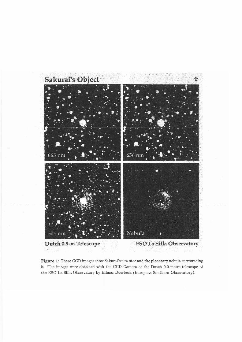
Figure 1: These CCD images show Sakurai's new star and the planetary nebula surrounding
it. The images were obtained with the CCD Camera at the Dutch 0.9-metre telescope at
the ESO La Silla Observatory by Hilmar Duerbeck (European Southern Observatory).
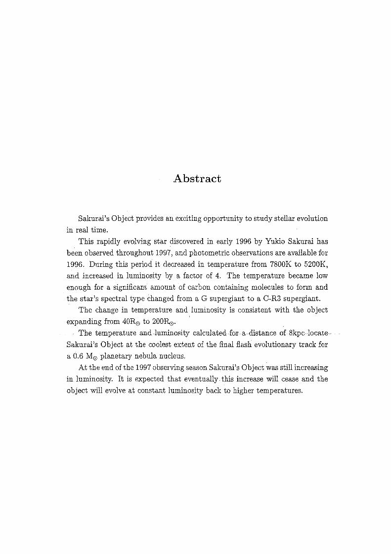
Abstract
Sakurai's Object provides an exciting opportunity to study stellar evolution
in real time.
This rapidly evolving star discovered in early 1996 by Yukio Sakurai has
been observed throughout 1997, and photometric observations are available for
1996. During this period it decreased in temperature from 7800K to 5200K,
and increased in luminosity by a factor of 4. The temperature became low
enough for a significant amount of carbon containing molecules to form and
the star's spectral type changed from a G supergiant to a C-R3 supergiant.
The change in temperature and luminosity is consistent with the object
expanding from 40R0 to 200R0 .
--- - The temperatme and-luminosity calculated -for-a-distan£e of 8kpc~locate
Sakurai's Object at the coolest extent of the final flash evolutionary track for
a 0.6 M0 planetary nebula nucleus.
At the end of the 1997 observing season Sakurai's Object was still increasing
in luminosity. It is expected that eventually. this increase will cease and the
object will evolve at constant luminosity back to higher temperatures.

vii
Contents
Figures xii
Tables Xlll
1 Introduction 2
1.1 What is Sakurai's Object 2
1.1.1 The photometric prehistory of Sakurai's Object 2
1. 2 The final flash scenario
1.3 Previously observed final flash objects
1.4 Planetary Nebulae
1.5 Observing Sakurai's Object
2 Observations
2.1 Photometry
2.2 Spectroscopy
2.3 Colours from low resolution spectra
3 Reduction and analysis techniques
3.1 The reduction of MRS spectra of Sakurai's Object
3.2 Continuum fitting
_3.3_ Line fitting andTadiaLv.elocities
3.4 Period analysis
2
3
5
6
8
8
13
15
18
18
18
2L 24
4 The physical characteristics of Sakurai's Object 25
4.1 Spectral classification 25
4.2 Determination of bolometric magnitudes 27
4.3 The distance to Sakurai's Object and the size of its planetary
nebula. 31
4.4 The temperature of Sakurai's Object
4.5 The radius of Sakurai's Object
4.6 Results
4. 7 Short term variability
4.8 Interpreting the observations as a final flash object
5 Sakurai's Object in context
5.1 A comparison with other final flash objects
5.1.1 The rise ...
33
33
34
35
37
40
40
40
viii

Contents
5.1.2 ... and fall of Sakurai's Object
5.1.3 The surrounding nebulosity
5.1.4 The origin of the R Coronae Borealis stars
5.2 Future observations
5.2.1 Dust
5.3 Summary : Sakurai's Object in 1996 and 1997
5.4 Postscript
6 Acknowledgements
References
A Reduction procedure
A.1 Image preparation
A.2 The dispersion solution
A.3 Scrunching
A.4 Sky subtraction
ix
40
41 41 41 42
42
43
45
46
48
48 49 50
50

Contents X
Figures
1. Pictures of Sakurai's Object from ESO La Silla. v
1.1 The evolutionary track of a final flash star 3
1.2 The light curve of FG Sagittae 4
1.3 The light curve of V854 Cen, an RCB star. 5
1.4 Infrared photometry of V605 Aquilae 6
2.1 A chart of Sakurai's Object, comparison and check stars. 9
2.2 Multicolour photometry of Sakurai's Object during 1997. 10
2.3 All the photometry available for 1996 and 1997. 11
2.4 All of the V photometry available for 1996 and 1997. 11
2.5 An example of a partially reduced MRS spectrum 14
2.6 A 150 1/mm MRS spectrum, with Cousins V and R filter func-
tions. 15
2.7 A calibration curve using stars of known (V-R) 16
3.1 A 150 1 mm-1 spectrum, with a continuum 19
3.2 The continuum fitting process. 20
3.3 Time sequences of the Na D and the Ha lines from MRS spectra. 22
3.4 A good fit to the Na D lines. 23
3.5 Duerbeck et al photometric data 24
4.1 A spectrum of Sakurai's Object compared with that of the
carbon star HD223392. 26
4.2 The spectrum of V605 Aquilae obtained by Lundmark in 1921. 27
4.3 The results of two different bolometric corrections. 29
4.4 The two possible positions of Sakurai's Object in the Galaxy. 32
4.5 The radius of Sakurai's Object as a function of time 34
4.6 Synthetic curves fitted to the short term variations of Sakurai's
Object. 37
4.7 The evolutionary track for a 0.6M0 final helium flash star. 38
4.8 The physical parameters of Sakurai's Object superimposed on
the evolutionary track for a 0.6M0 star. 38
5.1 The 1998 decline of Sakurai's Object. 44
A.1 A raw spectrum. 48
xi

Figures xii
A.2 The deviations from a linear fit in a dispersion solution. 49 A.3 A scrunched arc spectrum. 50
Tables xiii
Tables
2.1 The coordinates of Sakurai's Object, the comparison and two
check stars. 8
2.2 Photometric observations of Sakurai's Object made during 1997
at MJUO. 12
2.3 Medium Resolution Spectroscope approximate resolutions with
different filters and gratings. 13
2.4 Spectroscopic observations of Sakurai's Object 14
3.1 Measurements of the radial velocity of Sakurai's Object from
MRS spectra. 23
4.1 Absolute bolometric magnitudes calculated from the photo-
metric data using the normal supergiant and the carbon star
bolometric corrections, both for a distance of 8kpc. 30 4.2 The physical parameters of Sakurai's Object during 1996 and
1997. The first eight points are those used by Duerbeck et al
the rest are from the MJUO photometry 36
2
Chapter 1
Introduction
1.1 What is Sakurai's Object
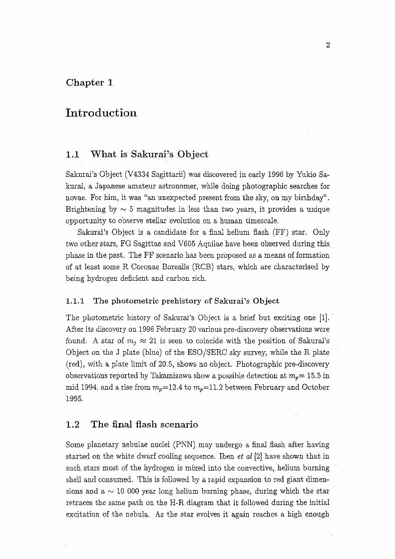
Sakurai's Object (V4334 Sagittarii) was discovered in early 1996 by Yukio Sa
kurai, a Japanese amateur astronomer, while doing photographic searches for
novae. For him, it was "an unexpected present from the sky, on my birthday" . Brightening by f'.J. 5 magnitudes in less than two years, it provides a unique opportunity to observe stellar evolution on a human timescale.
Sakurai's Object is a candidate for a final helium flash (FF) star. Only two other stars, FG Sagittae and V605 Aquilae have been observed during this phase in the past. The FF scenario has been proposed as a means of formation
of at least some R Coronae Borealis (RCB) stars, which are characterised by being hydrogen deficient and carbon rich.
1.1.1 The photometric prehistory of Sakurai's Object
The photometric history of Sakurai's Object is a brief but exciting one (1]. After its discovery on 1996 February 20 various pre-discovery observations were
found. A star of mj ~ 21 is seen to coincide with the position of Sakurai's
Object on the J plate (blue) of the ESO/SERC sky survey, while the R plate (red), with a plate limit of 20.5, shows no object. Photographic pre-discovery
observations reported by Takamizawa show a possible detection at mp= 15.5 in
mid 1994, and a rise from mp=12.4 to mp=11.2 between February and October '1995.
1. 2 The final flash scenario
Some planetary nebulae nuclei (PNN) may undergo a final flash after having
started on the white dwarf cooling sequence. Iben et al [2] have shown that in
such stars most of the hydrogen is mixed into the convective, helium burning shell and consumed. This is followed by a rapid expansion to red giant dimen
sions and a rv 10 000 year long helium burning phase, during which the star
retraces the same path on the H-R diagram that it followed during the initial excitation of the nebula. As the star evolves it again reaches a high enough
1.3. Previously observed final flash objects 3
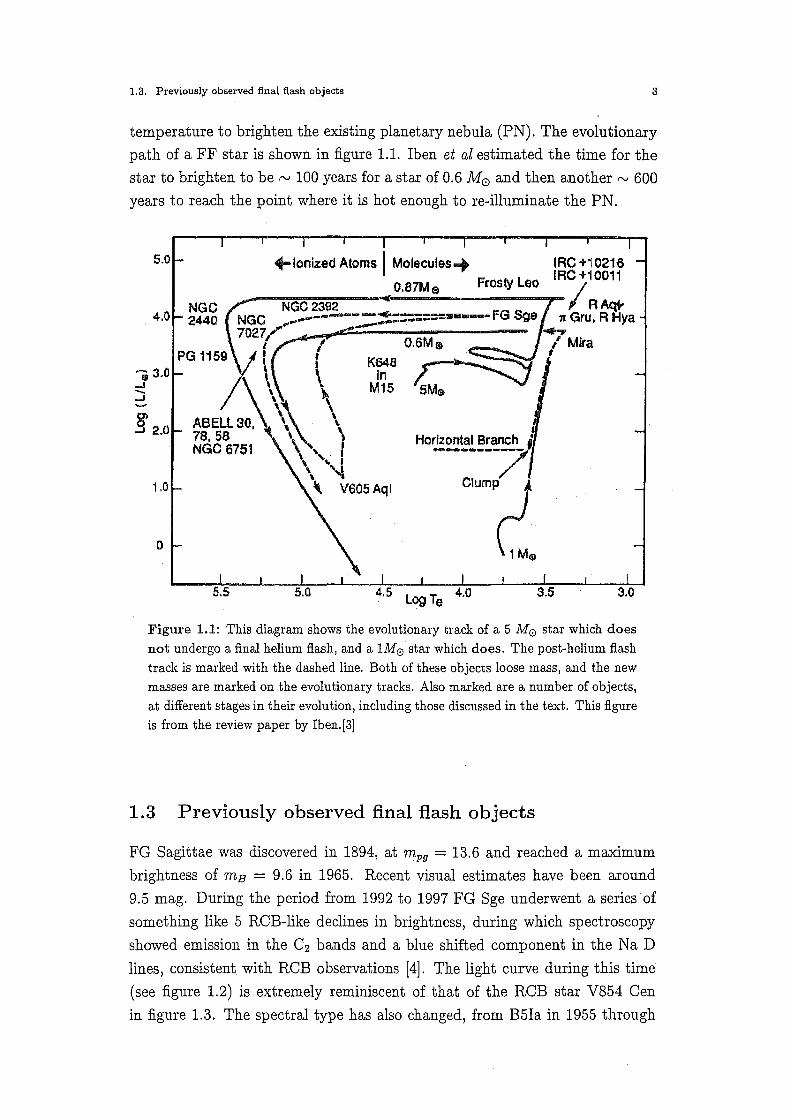
temperature to brighten the existing planetary nebula (PN). The evolutionary
path of a FF star is shown in figure 1.1. Iben et al estimated the time for the
star to brighten to be rv 100 years for a star of 0.6 M 0 and then another,....., 600
years to reach the point where it is hot enough to re-illuminate the PN.
1,0
0
Horizontal Branch ; -·-... ·---7 Clump~
1 M(j)
Figure 1.1: This diagram shows the evolutionary track of a 5 M 0 star which does
not undergo a final helium flash, and a 1M0 star which does. The post-helium flash
track is marked with the dashed line. Both of these objects loose mass, and the new masses are marked on the evolutionary tracks. Also marked are a number of objects, at different stages in their evolution, including those discussed in the text. This figure is from the review paper by Iben.[3]
1.3 Previously observed final flash objects
FG Sagittae was discovered in 1894, at mpg = 13.6 and reached a maximum
brightness of mB = 9.6 in 1965. Recent visual estimates have been around
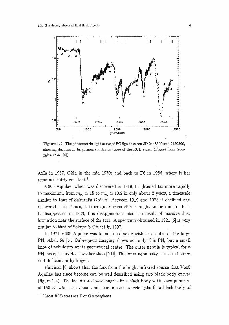
9.5 mag. During the period from 1992 to 1997 FG Sge underwent a series of
something like 5 RCB-like declines in brightness, during which spectroscopy
showed emission in the C2 bands and a blue shifted component in the Na D
lines, consistent with RCB observations [4]. The light curve during this time
(see figure 1.2) is extremely reminiscent of that of the RCB star V854 Cen
in figure 1.3. The spectral type has also changed, from B5Ia in 1955 through
1.3. Previously observed final flash objects
<> ':. . ~
I I 1 6
19915 1993.5 199-IS 1WS.S l99o.s
500 1000 1500 2000 2500
JD-2448000
Figure 1.2: The photometric light curve ofFG Sge between JD 2448500 and 2450500,
showing declines in brightness similar to those of the RCB stars. (Figure from Gon
zalez et al. [4])
4
A5Ia in 1967, G2Ia in the mid 1970s and back to F6 in 1986, where it has
remained fairly constant.1
V605 Aquilae, which was discovered in 1919, brightened far more rapidly
to maximum, from mp9 c::: 15 to mp9 c::: 10.2 in only about 2 years, a timescale
similar to that of Sakurai's Object. Between 1919 and 1923 it declined and
recovered three times, this irregular variability thought to be due to dust.
It disappeared in 1923, this disappearance also the result of massive dust
formation near the surface of the star. A spectrum obtained in 1921 [5] is very
similar to that of Sakurai's Object in 1997.
In 1971 V605 Aquilae was found to coincide with the centre of the large
PN, Abell 58 [5]. Subsequent imaging shows not only this PN, but a small
knot of nebulosity at its geometrical centre. The outer nebula is typical for a
PN, except that Ha is weaker than [NII]. The inner nebulosity is rich in helium
and deficient in hydrogen.
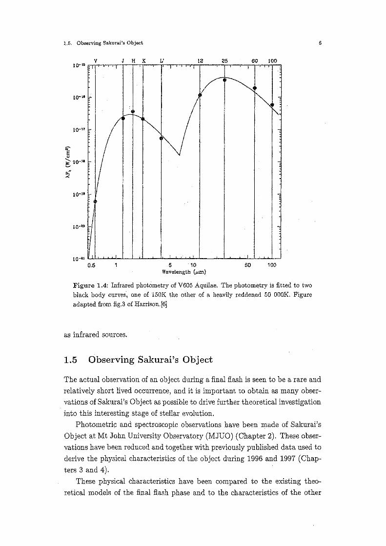
Harrison [6] shows that the flux from the bright infrared source that V605
Aquilae has since become can be well described using two black body curves
(figure 1.4). The far infrared wavelengths fit a black body with a temperature
of 150 K, while the visual and near infrared wavelengths fit a black body of
1 Most RCB stars are F or G supergiants
1.4. Planetary Nebulae 5
5.0
7.5 r-
:> 10.0 r-
12.5 r-
15.0 r-
r- 1.5
r- 1.0
r- 0.5
1
7000 8000 9000
JD (244 0000 + )
10000 0.0
11000
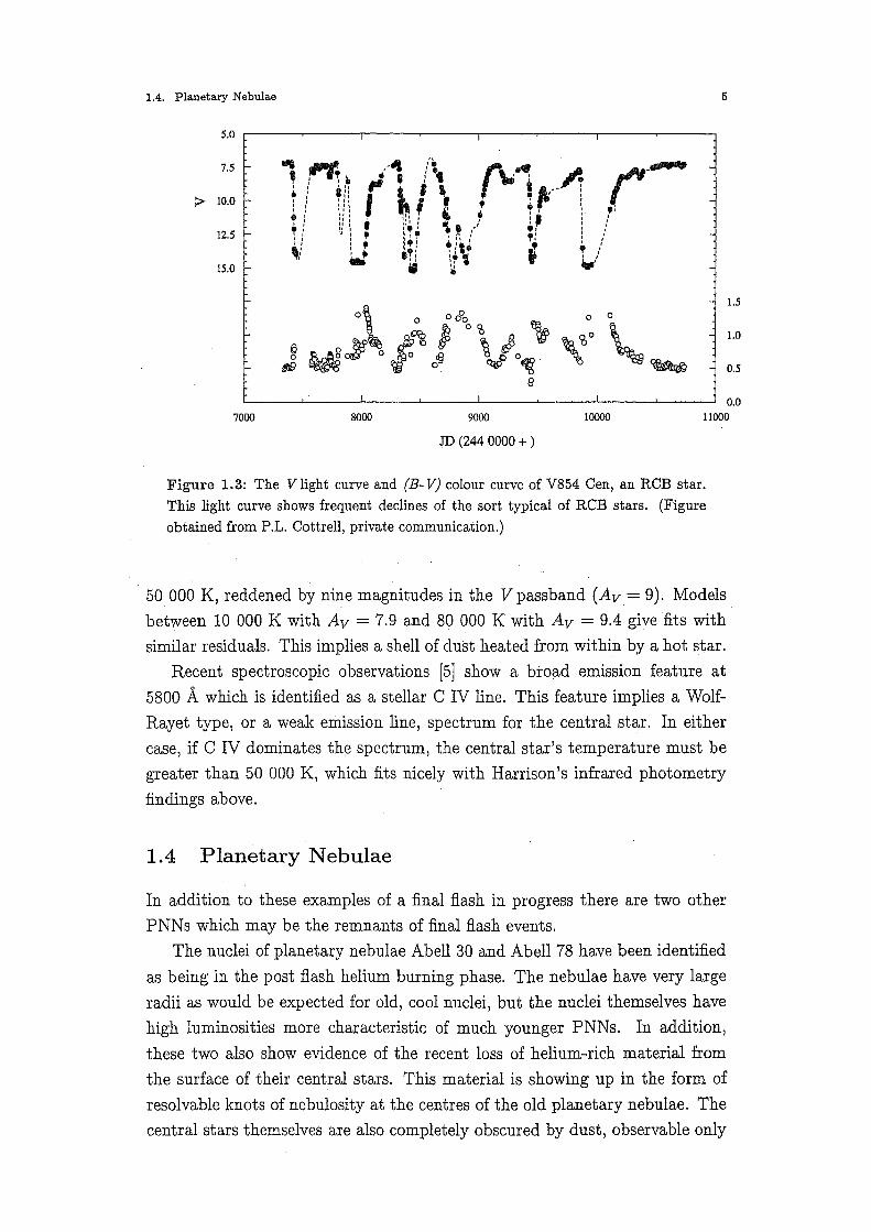
Figure 1.3: The V light curve and (B- V) colour curve of V854 Cen, an RCB star. This light curve shows frequent declines of the sort typical of RCB stars. (Figure
obtained from P.L. Cottrell, private communication.)
50 000 K, reddened by nine magnitudes in the V passband (Av = 9). Models
between 10 000 K with Av = 7.9 and 80 000 K with Av = 9.4 give fits with
similar residuals. This implies a shell of dust heated from within by a hot star.
Recent spectroscopic observations [5] show a broad emission feature at
5800 A which is identified as a stellar C IV line. This feature implies a Wolf
Rayet type, or a weak emission line, spectrum for the central star. In either
case, if C IV dominates the spectrum, the central star's temperature must be
greater than 50 000 K, which fits nicely with Harrison's infrared photometry
findings above.
1.4 Planetary Nebulae
In addition to these examples of a final flash in progress there are two other
PNNs which may be the remnants of final flash events.
The nuclei of planetary nebulae Abell 30 and Abell 78 have been identified
as being in the post flash helium burning phase. The nebulae have very large
radii as would be expected for old, cool nuclei, but the nuclei themselves have
high luminosities more characteristic of much younger PNNs. In addition,
these two also show evidence of the recent loss of helium-rich material from
the surface of their central stars. This material is showing up in the form of
resolvable knots of nebulosity at the centres of the old planetary nebulae. The
central stars themselves are also completely obscured by dust, observable only
1.5. Observing Sakurai's Object
v J H K L' 12 25 60 100 l I I I I
/~ ,_~
~ 10•11 f -;
......-- .......... "..:
~ 1::- -:
1::- -:
1::- "':
-:
1Q-21 I I I I . I
0.5 1 5 '10 50 100 Wavelength (~J.U~)
Figure 1.4: Infrared photometry of V605 Aquilae. The photometry is fitted to two black body curves, one of 150K the other of a heavily reddened 50 OOOK. Figure adapted from fig.3 of Harrison.[6]
as infrared sources.
1.5 Observing Sakurai's Object
6
The actual observation of an object during a final flash is seen to be a rare and
relatively short lived occurrence, and it is important to obtain as many observations of Sakurai's Object as possible to drive further theoretical investigation
into this interesting stage of stellar evolution.
Photometric and spectroscopic observations have been made of Sakurai's
Object at Mt John University Observatory (MJUO) (Chapter 2). These obser
vations have been reduced and together with previously published data used to
derive the physical characteristics of the object during 1996 and 1997 (Chap
ters 3 and 4).
These physical characteristics have been compared to the existing theo
retical models of the final flash phase and to the characteristics of the other
1.5. Observing Sakurai's Object 7
possible final flash stars (Chapters 4 and 5).
8
Chapter 2
0 bservations
2.1 Photometry
Photometry of Sakurai's Object commenced at MJUO in 1997 March. Obser
vations were made using the VERI filters similar to those described by Bessell
[7] with an EMI 9202B photomultiplier tube and the 0.6m Optical Crafts
man telescope. Observations in the U passband were initially attempted, but
abandoned after the object proved to be too faint in that passband for it to
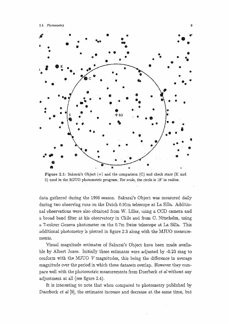
be worthwhile. The observations were made differentially with respect to a nearby comparison star. The position of the comparison star used, along with
the two check stars are shown in figure 2.1 and tabulated in table 2.1.
The· differential magnitudes of the variable and two check stars were then
transformed to the standard system using coefficients determined from obser
vations of E-Region standards [8]. This reduction to standard magnitudes was
done at MJUO using software written by Alan Gilmore.
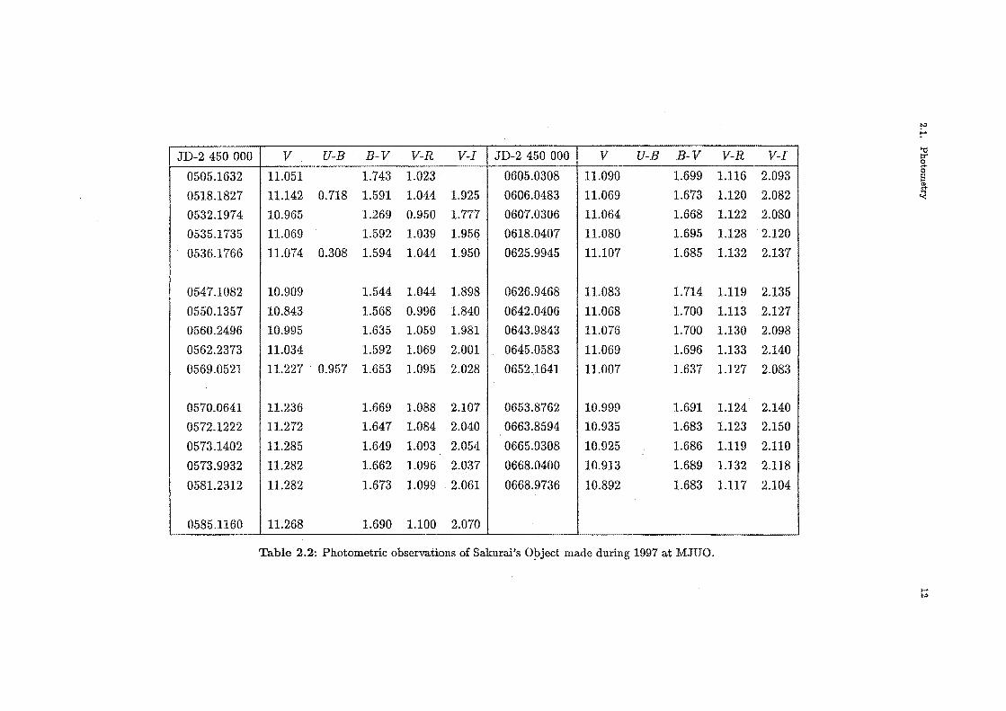
Each observation was taken twice and the mean of the observations is
used. Check star observations are used to determine the consistency of the
observations from night to night. The standard deviation of the V observations
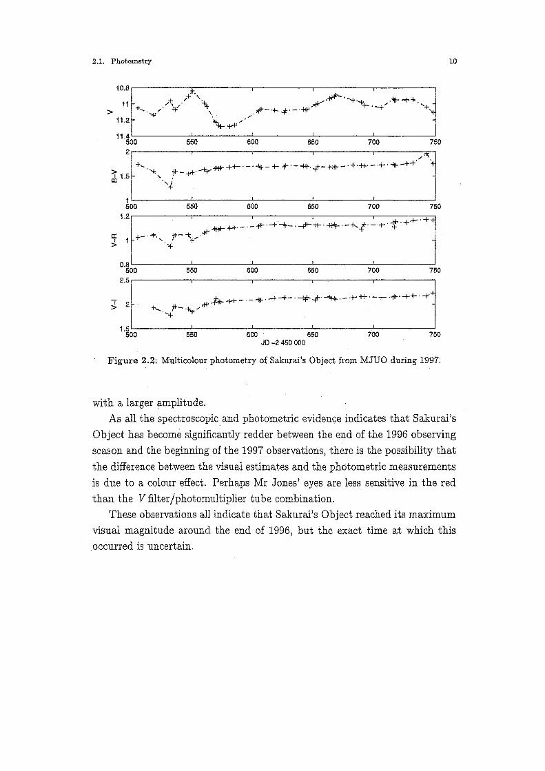
is 0.04mag, while that of the B- V, V-R, and V-I colours are all 0.03mag. The
observations are tabulated in table 2.2 and are plotted in figure 2.2. The point
at JD 2 450 532 is brighter and has lower colours than the points immediately
surrounding it. The observation report indicates a full moon on the night in
question, but no other reason to exclude this point, although it is possible that
the wrong star was observed.
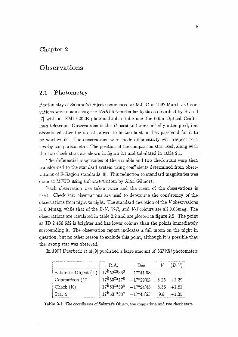
In 1997 Duerbeck et al [9] published a large amount of UBVRi photometric
R.A. Dec v (B- V)
Sakurai's Object ( +) 17h52m338 -17° 41'0811
Comparison (C) 17h53m178 -17°29'0211 8.25 +1.29
Check (K) 17h53m59s -17°24'4511 8.36 +1.81
Star 5 17h53m38s -17° 4315311 9.8 +1.35
Table 2.1: The coordinates of SakuraPs Object, the comparison and two check stars.
2.1. Photometry 9 , • • • • . ...
• • • • • • • •• .. • Ill • • • • • • • • • • .• • • • • .. • •• • • ' • K • • • • I • • • • • •• •
" • • .. • . • • • • • • • • • • • • • • • • • • • •• • . - • • • • • • • • • • • • • • • • • • • •• +so • • • • • • • • • • ' • • • • • • • • • • • • • •
• I
•• • • • • • • • • • • .. ,. • • • • • • • •
Figure 2.1: Sakurai's Object(+) and the comparison (C) and check stars (K and 5) used in the MJUO photometric program. For scale, the circle is 18' in radius.
data gathered during the 1996 season. Sakurai's Object was measured daily
during two observing runs on the Dutch 0.91m telescope at La Silla. Additio
nal observations were also obtained from W. Liller, using a CCD camera and a broad band filter at his observatory in Chile and from C. Nitschelm, using
a 7-colour Geneva photometer on the 0.7m Swiss telescope at La Silla. This additional photometry is plotted in figure 2.3 along with the MJUO measurements.
Visual magnitude estimates of Sakurai's Object have been made availa
ble by Albert Jones. Initially these estimates were adjusted by -0.23 mag to conform with the MJUO V magnitudes, this being the difference in average
magnitude over the period in which these datasets overlap. However they com
pare well with the photometric measurements from Duerbeck et al without any adjustment at all (see figure 2.4).
It is interesting to note that when compared to photometry published by
Duerbeck et al [9], the estimates increase and decrease at the same time, but
2.1. Photometry 10
> 11.2
550 600 650 700 750
> cb 1.5
1~--------~--------~--------~--------~--------~ 500 550 600 650 700 750
1.2 .---------r---------.----. -----...... ..-----.---#--· +-rl-,..--' +'·-:1-j. #- ++·-.--Ill-.-+,._. -t'' *'". -li'4-. -+....t·- ·+-' + .
a:: +-·+._ t-·'\ ·"*' >I 1 ' +_..
':f
0.8 '------"'-------.J....:..-----...__ ____ _,__ ______ _, 500 550 600 650 700 750
~ 2-:r. +- f ~,* ~#- ~~ ~+~~-~ - +* ~~ ~ +Hj 1.5~------~-------~-------~-----~---~
500 550 600 650 700 750 JD -2 450 000
Figure 2.2: Multicolour photometry of Sakurai's Object from MJUO during 1997.
with a larger amplitude. As all the spectroscopic and photometric evidence indicates that Sakurai's
Object has become significantly redder between the end of the 1996 observing
season and the beginning of the 1997 observations, there is the possibility that
the difference between the visual estimates and the photometric measurements
is due to a colour effect. Perhaps Mr Jones' eyes are less sensitive in the red
than the V filter/photomultiplier tube combination. These observations all indicate that Sakurai's Object reached its maximum
visual magnitude around the end of 1996, but the exact time at which this ,occurred is uncertain.
2.1. Photometry
8.5
9
9.5 0
~0 10 "" 00 0
10.5 811'0 =l 11
~ 11.5
12 dt>~o 0
12.5 0
13
13.5 100 200 300 400 500 600 700 800
JD-2450 000
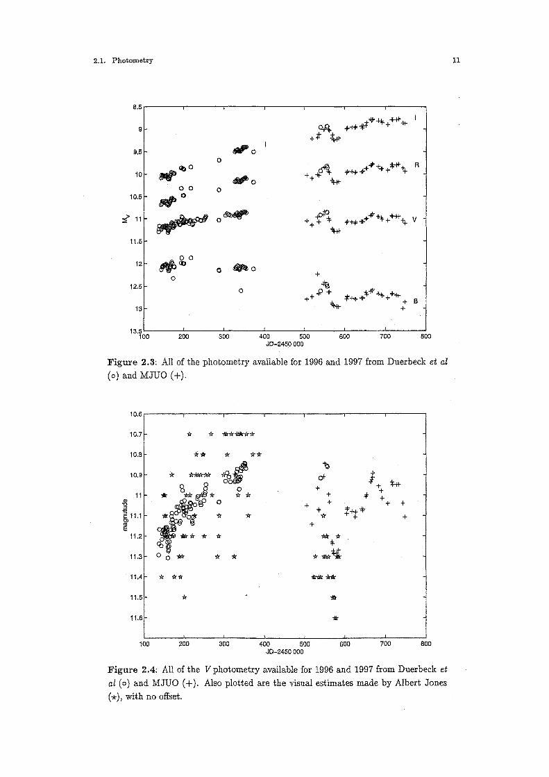
Figure 2.3: All of the photometry available for 1996 and 1997 from Duerbeck et al
(o) and MJUO (+).
10.6r-----.-----r-----.----.,.------,.----,------,
10.7 "* 10.8 ** "* "*"* "b
ol" J + ** + + *
+ +
+ + + + • t++ -JF * + +
10.9
11
+ 11.2 *k'k
* 11.3 *~*t 11.4 "* "** 'flrlk **
11.5 * * 11.6 *
100 200 300 400 500 600 700 800 JD-2450000
Figure 2.4: All ofthe Vphotometry available for 1996 and 1997 from Duerbeck et al ( o) and MJUO ( +). Also plotted are the visual estimates made by Albert Jones (*), with no offset.
11
JD-2 450 000 v U-B B-V V-R V-I JD-2 450 000 v U-B B-V 0505.1632 11.051 1.743 1.023 0605.0308 11.090 1.699
0518.1827 11.142 0.718 1.591 1.044 1.925 0606.0483 11.069 1.673
0532.1974 10.965 1.269 0.950 1.777 0607.0306 11.064 1.668
0535.1735 11.069 1.592 1.039 1.956 0618.0407 11.080 1.695
0536.1766 11.074 0.308 1.594 1.044 1.950 0625.9945 11.107 1.685
0547.1082 10.909 1.544 1.044 1.898 0626.9468 11.083 1.714
0550.1357 10.843 1.568 0.996 1.840 0642.0406 11.068 1.700
0560.2496 10.995 1.635 1.059 1.981 0643.9843 11.076 1.700
0562.2373 11.034 1.592 1.069 2.001 0645.0583 11.069 1.696
0569.0521 11.227 0.957 1.653 1.095 2.028 0652..1641 11.007 1.637
0570.0641 11.236 1.669 1.088 2.107 0653.8762 10.999 1.691
0572.1222 11.272 1.647 1.084 2.040 0663.8594 10.935 1.683
0573.1402 11.285 1.649 1.093 2.054 0665.9308 10.925 1.686
0573.9932 11.282 1.662 1.096 2.037 0668.0400 10.913 1.689
0581.2312 11.282 1.673 1.099 2.061 0668.9736 10.892 1.683
0585.1160 11.268 1.690 1.100 2.070
Table 2.2: Photometric observations of Saknrai's O?ject made during 1997 at MJUO.
V-R 1.116
1.120
1.122
1.128
1.132
1.119
1.113
1.130
1.133
1.127
1.124
1.123
1.119
1.132
1.117
V-I 2.093
2.082
2.080
2.120
2.137
2.135
2.127
2.098
2.140
2.083
2.140
2.150
2.110
2.118
2.104
!"' ~
'"d [
!
...... ..,
2.2. Spectroscopy 13
2.2 Spectroscopy
The spectroscopic observations were made with the Medium Resolution Spec
trograph (MRS) on the 1m telescope at MJUO. The spectrograph was used
with three different gratings and two filters. All of the spectra have been
obtained using a slit of 150,um by 30 mm, which corresponds to 2.3 x 460
arc seconds on the sky. This long slit option allows sky subtraction to be
performed during the reduction procedure.
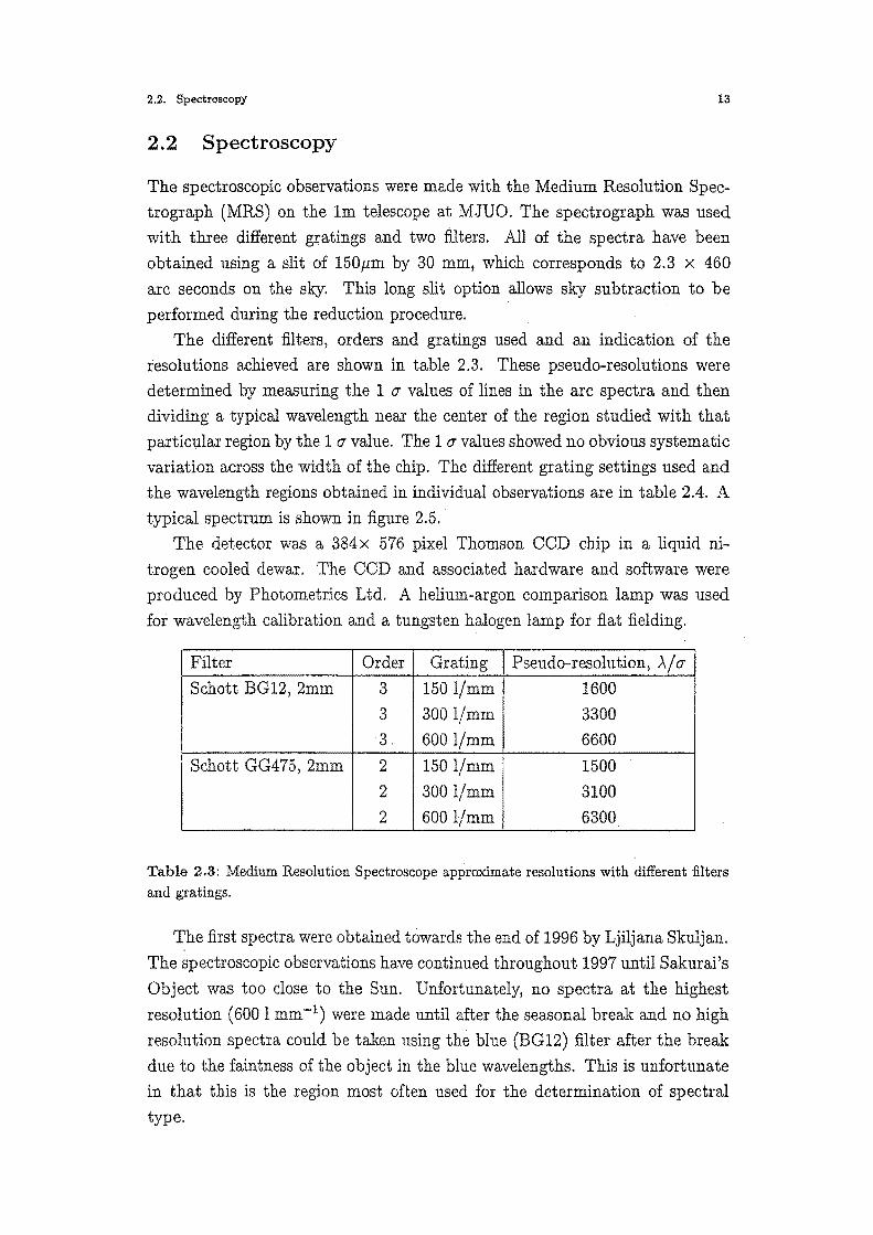
The different filters, orders and gratings used and an indication of the
resolutions achieved are shown in table 2.3. These pseudo-resolutions were determined by measuring the 1 u values of lines in the arc spectra and then
dividing a typical wavelength near the center of the region studied with that particular region by the 1 u value. The 1 u values showed no obvious systematic
variation across the width of the chip. The different grating settings used and
the wavelength regions obtained in individual observations are in table 2.4. A
typical spectrum is shown in figure 2.5.
The detector was a 384x 576 pixel Thomson CCD chip in a liquid ni
trogen cooled dewar. The CCD and associated hardware and software were
produced by Photometries Ltd. A helium-argon comparison lamp was used
for wavelength calibration and a tungsten halogen lamp for flat fielding.
Filter Order Grating Pseudo-resolution, A/ u
Schott BG12, 2mm 3 150 1/mm 1600
3 300 1/mm 3300
3 600 1/mm 6600
Schott GG475, 2mm 2 150 1/mm 1500
2 300 1/mm 3100 2 600 ljmm 6300
Table 2.3: Medium Resolution Spectroscope approximate resolutions with different filters and gratings.
The first spectra were obtained towards the end of 1996 by Ljiljana Skuljan.
The spectroscopic observations have continued throughout 1997 until Sakurai's
Object was too close to the Sun. Unfortunately, no spectra at the highest
resolution (600 1 mm-1) were made until after the seasonal break and no high
resolution spectra could be taken using the blue (BG12) filter after the break
due to the faintness of the object in the blue wavelengths. This is unfortunate in that this is the region most often used for the determination of spectral
type.
2.2. Spectroscopy
de.te JD-2 450 000 .\ from to noise grating filter tilt connnenta 27/9/96 353.5 5600 6800 4% 300 GG475 255 27/9/96 353.5 3800 4500 28% 300 BG12 255 Tao few counts 28/9/96 354.5 5000 7300 2% 150 GG475 35 30/9/96 356.5 3700 4500 10% 300 BG12 255 30/9/96 356.5 5700 6800 4% 300 GG475 255 9/10/96 365.5 5700 6800 4% 300 GG475 255
Se08ona.l Break
10/3/97 517.5 5700 6800 4% 300 GG475 255 12/3/97 519.5 5000 7300 2% 150 GG475 35 14/3/97 521.5 5700 6300 8% 600 GG475 660 This is the first of the hig-
hest resolution spectra.. 6/4/97 544.5 5610 6300 4% 300 GG475 210
8/4/97 546.5 5700 6300 8% 600 GG475 660 1/5/97 569.5 4600 5250 2.5% 600 GG475 580 2/5/97 570.5 6200 6800 3% 600 GG475 740
2/5/97 570.5 1100 7700 4% 600 GG475 870 3/5/97 571.5 5200 5800 5% 600 GG475 580 3/5/97 571.5 5700 6300 8% 600 GG475 660 3/5/97 571.5 6200 6800 4% 600 GG475 740 4/5/97 572.5 7100 7700 4% 600 GG475 870 4/5/97 572.5 3500 4800 6% 150 BG12 35 No counts below 3900 A 4/5/97 572.5 5000 7300 2% 150 GG475 35 6/6/97 605.5 5700 6300 4% 600 GG475 660 3/8/97 663.5 5000 7300 2% 150 GG475 35 3/8/97 663.5 3500 4800 16% 150 BG12 35 3/8/97 663.5 5610 6300 4% 300 GG475 210 3/8/97 663.5 5700 6800 2% 300 GG475 255
13/9/97 700.5 5000 7300 2% 150 GG475 35 OK 13/9/97 700.5 5100 6150 5% 300 GG475 210 Problems with 13/9/97 700.5 5700 6800 4% 300 GG475 255 bright moon
13/9/97 700.5 6400 7400 4% 300 00475 300 n.nd clouds 14/9/97 701.5 5700 6300 ? 600 GG475 660 Moon, no c:::loud.s
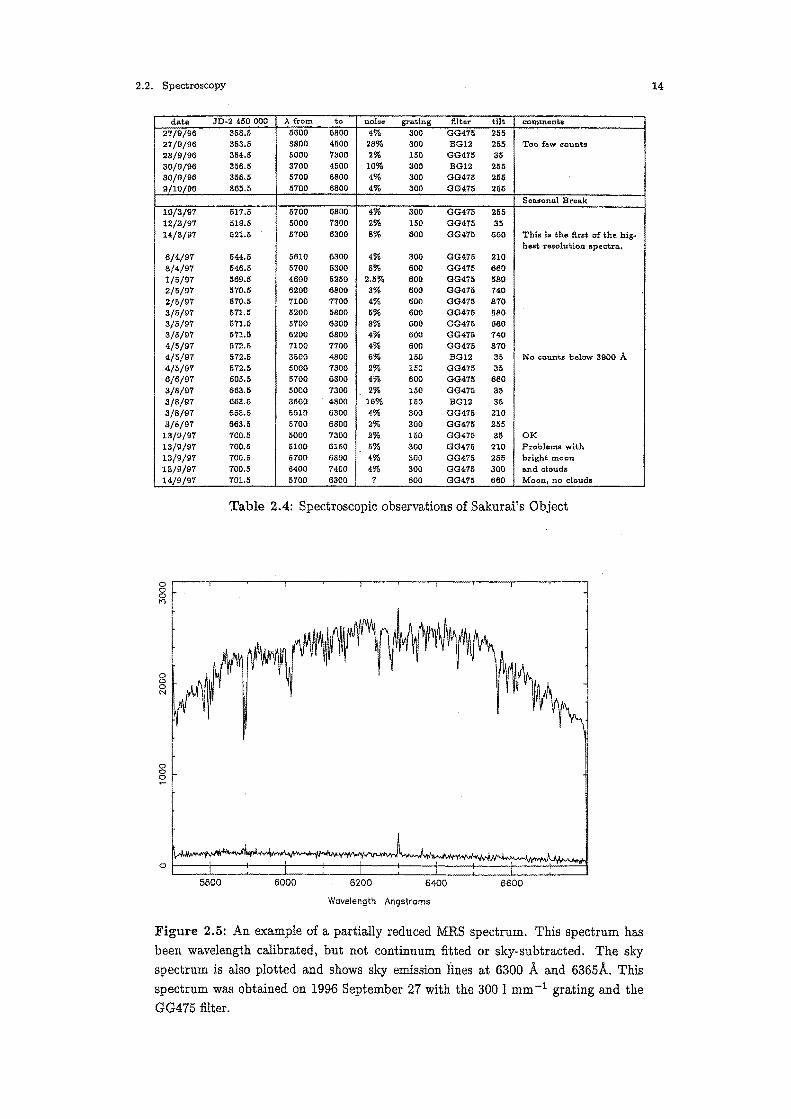
Table 2.4: Spectroscopic observations of Sakurai's Object
0 r-----.-----~---.----~-----.----~-----r-----.-----.-----.----, 0 0 t"l
8 0 N
8 0
Wavelength Angstroms
Figure 2.5: An example of a partially reduced MRS spectrum. This spectrum has
been wavelength calibrated, but not continuum fitted or sky~subtracted. The sky
spectrum is also plotted and shows sky emission lines at 6300 A and 6365A. This
spectrum was obtained on 1996 September 27 with the 300 I mm-1 grating and the
GG475 filter.
14
2.3. Colours from low resolution spectra. 15
The spectra obtained throughout the 1997 observing season have not shown
any significant changes since the molecular bands appeared during the 1996/97
seasonal break. For a comparison to figure 2.5 see figure 3.1, a 1997 spectrum.
2.3 Colours from low resolution spectra
Spectroscopic observations were obtained late in 1996, but photometric moni
toring at MJUO did not start until the 1997 season. Before the publication of
Duerbeck et al's [9] photometric data for 1996 there was no colour information
available, although visual brightness estimates were available. Information
about the colour of the object was needed in order to estimate its temperature. This section describes how a reasonable {V-R) colour estimate was found
from low resolution spectra.
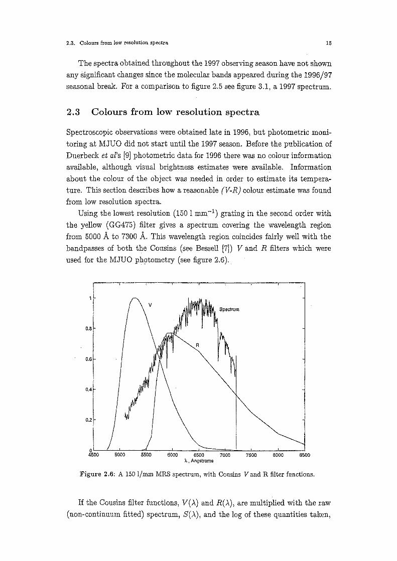
Using the lowest resolution (150 l mm-1 ) grating in the second order with
the yellow (GG475) filter gives a spectrum covering the wavelength region
from 5000 A to 7300 A. This wavelength region coincides fairly well with the
bandpasses of both the Cousins (see Bessell [7}) V and R filters which were
used for the MJUO ph9tometry (see figure 2.6).
0.8
0.6
0.4
0.2
0~-L~-----d----~----~~~==~---L-----L----~ 4500 5000 5500 6000 6500 7000 7500 8000 8500
A. , Angstroms
Figure 2.6: A 150 1/mm MRS spectrum, with Cousins V and R filter functions.
If the Cousins filter functions, V(.A) and R(.A), are multiplied with the raw
(non-continuum fitted) spectrum, S(.A), and the log of these quantities taken,
2.3. Colours from low resolution spectra. 16
then values fv and fR are obtained which are proportional to the photometric measurements of V and R, with a factor due to the instrumental response of
the spectrograph.
The values fv = f>. S(.\)V(.\) and fR = f>. S(.\)R(.\) were calculated for some RCB stars and 1997 observations of Sakurai's Object for which quasi
simultaneous V and R photometry and MRS spectroscopy were available. A simple rectangular numerical integration over a large number of points was
used. Since the spectra were not taken under photometric conditions these two
numbers fv and !Rare fairly meaningless by themselves. However the quantity
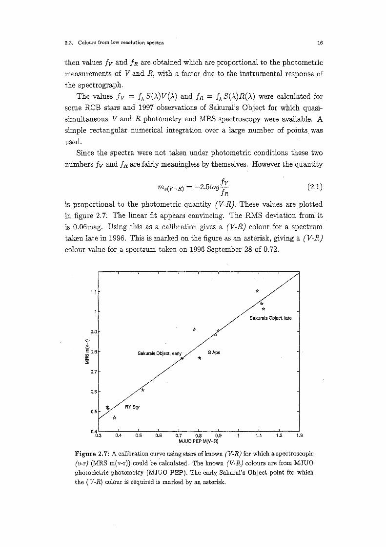
fv ms(V-R) = -2.5log fR (2.1)
is proportional to the photometric quantity (V-R). These values are plotted
in figure 2. 7. The linear fit appears convincing. The RMS deviation from it ~
is 0.06mag. Using this as a calibration gives a (V-R) colour for a spectrum
taken late in 1996. This is marked on the figure as an asterisk, giving a (V-R)
colour value for a spectrum taken on 1996 September 28 of 0.72.
1.1
0,9
I *
* * Sakurais Object, late
E 0.8 SAps ~ ~
0.7
0.6 * RYSgr
0.5
* 0.4 '------'------'----'----'-----l.--..l..----1--.....--'L..----'----'
0.3 0.4 0.5 0.6 0.7 0.8 0.9 1.1 1.2 1.3 MJUO PEP M(V-R)
Figure 2. 7: A calibration curve using stars of known (V-R) for which a spectroscopic (v-r} (MRS m(v-r)) could be calculated. The known (V-R) colours are from MJUO photoeletric photometry (MJUO PEP). The early Sakurai's Object point for which the ( V-R) colour is required is marked by an asterisk.
2.3. Colours from low resolution spectra 17
This procedure has since become redundant with the publication of 1996
photometry by Duerbeck et al. The new photometry does however provide
confirmation that the technique is a viable one, as for their last points in 1996,
covering the September period the mean (V-R) is 0.75.

18
Chapter 3
Reduction and analysis techniques
3.1 The reduction of MRS spectra of Sakurai's Object
These spectra were reduced using the Figaro package. The reduction procedure
follows more or less the procedure devised for the reduction of echelle spectra
[10]. Some aspects of the reduction procedure more specific to the spectra
of late-type carbon stars are discussed here. A more detailed outline of the
general procedure used is in appendix A.
3.2 Continuum fitting
Sakurai's Object is a late-type star with so many absorption lines present that
the position of the continuum is difficult to determine. In addition to this,
in the period since observations were started at Mt John, molecular bands
of various carbon compounds have developed, further distorting the flux dis
tribution of this star. This all makes it very difficult to identify any sort of
continuum at all. The continuum would be expected to approximate a black
body curve dependent on the temperature of the star, with the instrumental
profile due to filters, the detector response and the off-blaze-angle response of
the grating superimposed. The continuum also falls away at both ends due to
instrumental effects such as vignetting within the spectrograph. As the spec
trum shows no obvious emission features, there would be no points significantly
above the continuum.
An approximation has been made based upon the shape of the flat field
lamp spectra (somewhat cooler than Sakurai's Object) and the velocity stan
dard spectra (somewhat hotter than Sakurai's Object and with fewer lines).
Lower resolution spectra can also provide some helpful information, as they
cover a sufficiently broad region of the spectrum to extend beyond the mole
cular bands. The Figaro subroutine CFIT allows the user to place points on
the spectrum through which a spline is fitted.
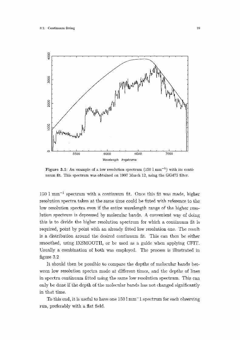
To achieve consistency the 150 1 mm-1 spectra were fitted first, on the
assumption that the localised depressions due to bands would have a smal
ler effect on the overall shape of the spectrum. Figure 3.1 shows one such
3.2. Continuum fitting
0
8 r-~~~~--~~~~----~~~~~--~~~--~,-~~--"<t'
0 0 0 I')
0 0 0 N
0 0 0 ~
5500 6000 6500 7000
Wavelength Angstroms
Figure 3.1: An example of a low resolution spectrum (150 l mm-1 ) with its conti
nuum fit. This spectrum was obtained on 1997 March 12, using the GG475 filter.
19
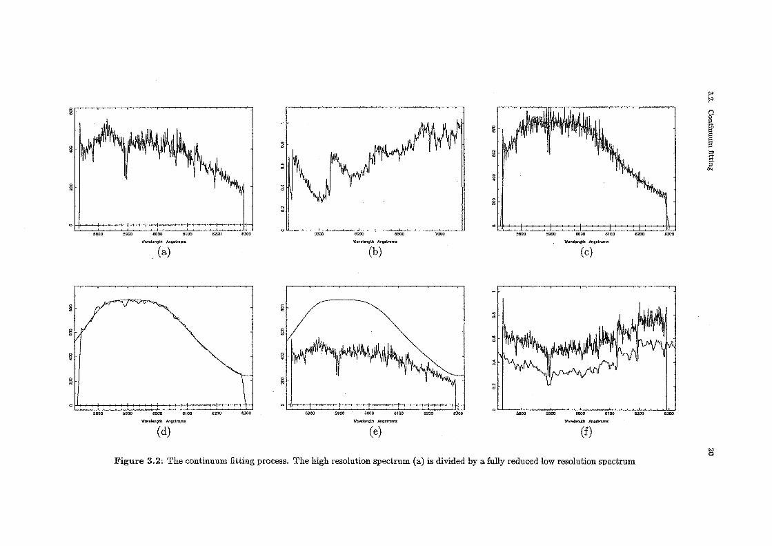
150 1 mm - 1 spectrum with a continuum fit. Once this fit was made, higher
resolution spectra taken at the same time could be fitted with reference to the
low resolution spectra even if the entire wavelength range of the higher reso
lution spectrum is depressed by molecular bands. A convenient way of doing
this is to divide the higher resolution spectrum for which a continuum fit is
required, point by point with an already fitted low resolution one. The result
is a distribution around the desired continuum fit. This can then be either
smoothed, using IXSMOOTH, or be used as a guide when applying CFIT.
Usually a combination of both was employed. The process is illustrated in
figure 3.2
It should then be possible to compare the depths of molecular bands bet
ween low resolution spectra made at different times, and the depths of lines
in spectra continuum fitted using the same low resolution spectrum. This can
only be done if the depth of the molecular bands has not changed significantly
in that time.
To this end, it is useful to have one 150 l mm-1 spectrum for each observing
run, preferably with a flat field.
g
~
~ ~ d
d
~ ~ d
~ :;!
5a00 5900 6000 5100 6200 6JOO 5500 6000 6500 1000 5800 5900 5000 6100 6200
Wcvetengtk Mg::~trotns Wavelength Anp;troins WovdMgth Ang•lrctm~
(a) (b) (c)
g :;!
g d
~ ~ ~
d
~ ~ :;!
5800 5900 6000 5100 6200 6JOO 5600 5900 6000 5100 6200 6300 5800 5900 6000 5100 5200
Wove1ength An{Pltums Wova:lemgth AAgstnlms ~An~tr-omw
(d) (e)
Figure 3.2: The continuum fitting process. The high resolution spectrum (a) is divided by a fully reduced low resolution spectrum
6JOO
6300
t» ~
Q
~ ~ l;l? .,.. s·
(Jq
tv 0
3.3. Line fitting and radial velocities 21
Another way to cope with this problem will be to take spectra of metal deficient stars of similar spectral types, which will hopefully give an almost line-free continuum.
3. 3 Line fitting and radial velocities
Spectra obtained using the MRS are obviously not ideal for the determination
of very precise radial velocities but reasonable estimates can be obtained from
the highest resolution spectra. The Ha and N a D lines have been used in this analysis because they are easily identified in the crowded spectra of Sakurai's Object.
The positions of the Ha and Na D lines were determined by fitting Gaussian profiles to them using the package GAUSS in Figaro. This package allows the
user to fit multiple Gaussian profiles to subsets of spectra. The user first defines
a continuum or, in the case of Sakurai's Object, a pseudo-continuum by fitting a low order polynomial to selected parts of the spectrum. Then Gaussians are
approximately placed on the line or blend to be fitted. The program optimises the fit and returns the central wavelength, width and height of the optimised
Gaussian profiles. GAUSS fits to lines in the helium argon comparison lamp spectra show
a maximum uncertainty of about 0.2 A at the highest resolution, which is equivalent to a Doppler shift of± 10 km/s at the position of the Na D lines.
Repeated fits with slightly varied initial conditions ( eg, continuum position)
show an additional uncertainty of~ 0.1 A in using GAUSS to measure the position of a spectral line.
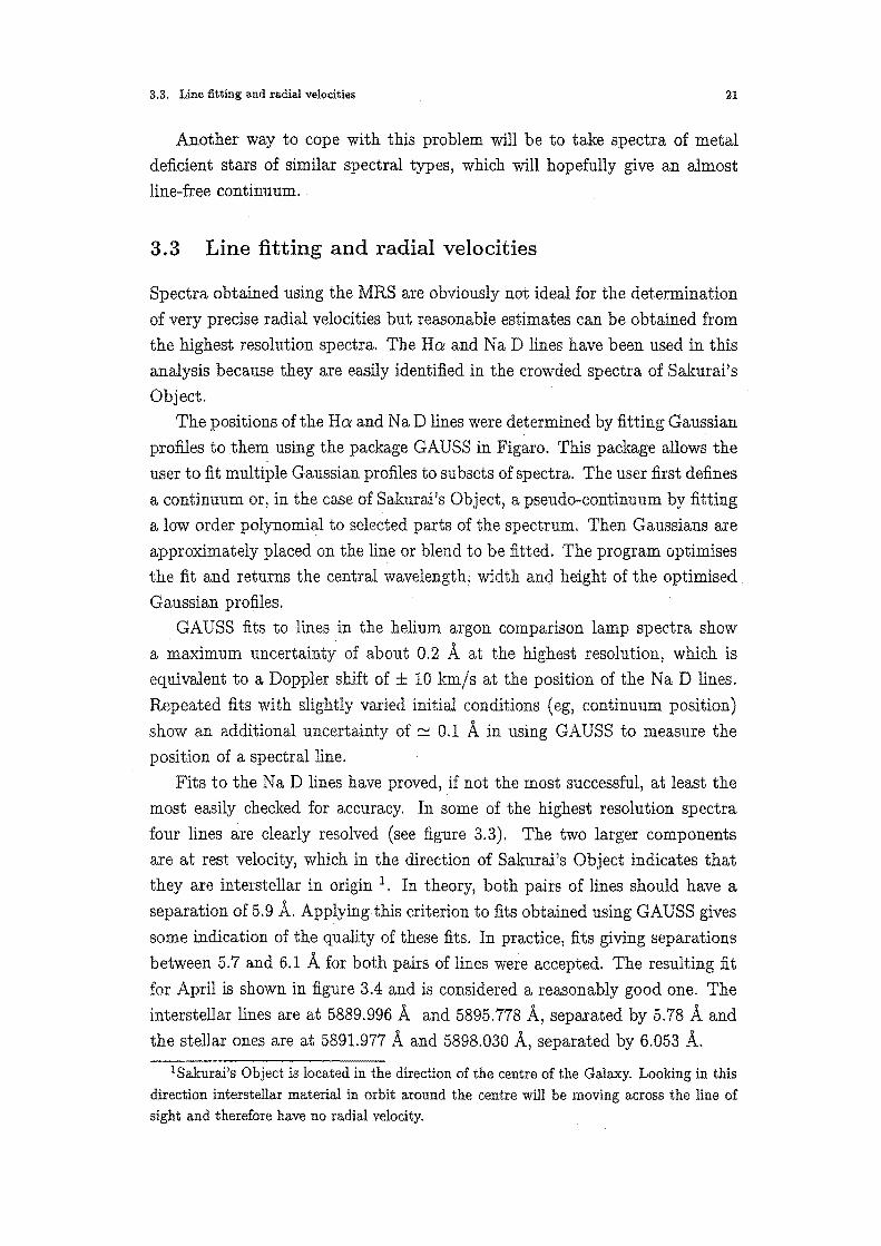
Fits to the N a D lines have proved, if not the most successful, at least the most easily checked for accuracy. In some of the highest resolution spectra
four lines are clearly resolved (see figure 3.3). The two larger components are at rest velocity, which in the direction of Sakurai's Object indicates that
they are interstellar in origin 1. In theory, both pairs of lines should have a
separation of 5.9 A. Applying this criterion to fits obtained using GAUSS gives
some indication of the quality of these fits. In practice, fits giving separations between 5.7 and 6.1 A for both pairs of lines were accepted. The resulting fit
for April is shown in figure 3.4 and is considered a reasonably good one. The
interstellar lines are at 5889.996 A and 5895.778 A, separated by 5.78 A and the stellar ones are at 5891.977 A and 5898.030 A, separated by 6.053 A.
1Sakurai's Object is located in the direction of the centre of the Galaxy. Looking in this direction interstellar material in orbit around the centre will be moving across the line of sight and therefore have no radial velocity.
3.3. Line fitting and radial velocities
NaO Ha
~8.'::-:70~'---':::58'::-:ao~--':':'589:-:'0 ~~5:-:~:9ooc:'-'-""""-':5::"91-::-0 ~""'::'5920 ~5~40~'---':::65~50~~656:-:'0~~.~57:-:'0~~6~58~0~~6590
Wavelength Angstroms Wavelength Angstroms ·
Figure 3.3: Time sequences of the Na D lines Ha lines from MRS spectra. In all of
these spectra the local continuum has been normalised to 1 in arbitrary flux units.
They have then been offset in steps of 0.2. The Ha lines have been plotted on a
larger scale. Thin lines indicate a 300 l mm-1 spectrum while thick ones indicate a 600 1 mm-1 spectrum. Differences in the appearance of the later 600 l mm-1 spectra
compared to the earliest ones are due to a poorly focussed spectrograph.
22
The best fits to the Na D and Ha lines show radial velocities of between
86 and 125 km s-1 (table 3.1). Within the estimated uncertainties this is in
agreement with the radial velocities of 115 km s-1 [1] and 125 km s-1 [9] ob
tained by other researchers. These velocities appear to have increased slightly
over the period during which these measurements were made. Unfortunately
Sakurai's Object is too dim for higher resolution spectroscopy at MJUO using
the echelle spectrograph.

3. 3. Line fitting and radial velocities
date grating line meas. A shift velocity lmm-1 A A km s-1
1996 Sept 27 300 Ha 6564.746 1.896 86±15
1996 Oct 09 300 Ha 6564.879 2.029 93 ± 15
1997 March 10 300 Ha 6565.368 2.518 115 ± 30
1997 March 14 600 Na D1 5898.003 2.063 104 15
NaD2 5892.147 2.174 110 15
1997 April 08 600 NaD1 5898.030 2.090 106 ± 15
NaD2 5891.977 2.004 102 ± 15
1997 May 02 600 Ha 6565.192 2.342 107 ± 15
1997 May 03 600 NaD1 5898.307 2.387 120 15
NaD2 5892.226 2.253 114± 15
1997 Aug 03 300 Ha 6565.375 2.529 116 ± 30
1997 Sept 14 600 NaD1 5892.324 2.351 120 ± 20
NaD2 5898.402 2.462 125 ± 20
Table 3.1: Measurements of the radial velocity of Sakurai's Object from MRS spectra.
"'~ -co :::1
.0 (.)
tO 0
NaD
* ' * *.
*·
*
* *
23
5880 5900 5910 5920
Wavelength Angstroms
Figure 3.4: A moderately good fit to the Na D lines in a high resolution MRS
spectrum. Four Gaussian curves have been used to model these lines from 1997 April.
3.4. Period analysis 24
3.4 Period analysis
Both the MJUO data and the photometric data published by Duerbeck et al fot
1997 have been analysed for periodicities of less than 100 days. This analysis
was done using the Fourier transform code T7, which uses a Lomb-Scargle
algorithm. This algorithm is widely used in astronomical work as it deals with
data on a point by point basis, and so does not require that the data be evenly
spaced in time as Fast Fourier transform algorithms do. The original code for
T7 was published by Press and Teukolsky [11] and has since been developed in
the Astronomy Research Group at the University of Canterbury by a number
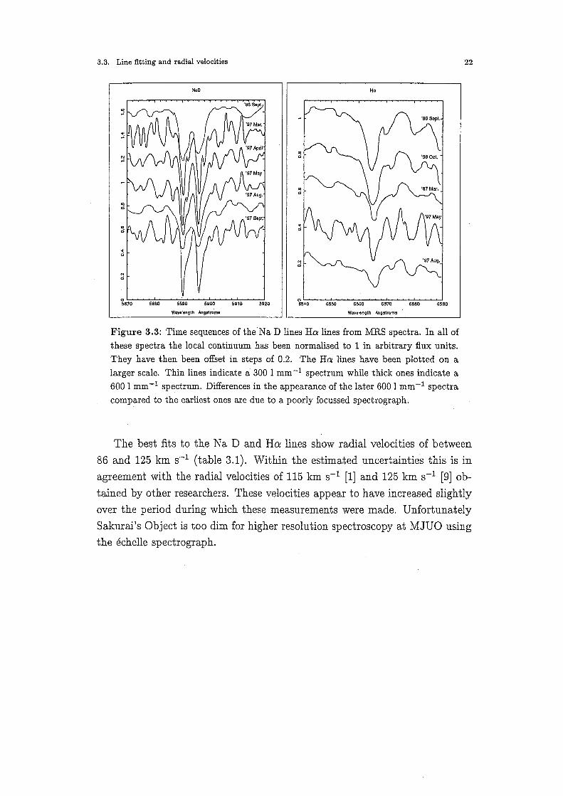
of researchers. Before the data from Duerbeck et al could be analysed in this way it was
necessary to remove the increasing trend of the data as the star became brigh
ter. This was done by subtracting a linear fit from the data. The unsmoothed
data, and the fit used, are plotted in the top panel of figure 3.5 and the smoo
thed data that was finally used is in the bottom panel. It was not necessary
to smooth the MJUO data in a similar fashion because there was no trend in
that data set. The results from this period analysis are presented in chapter 4.
10.8
11 >
E . 11.1
11.3
150 200 250 300 350
-0.2.----.-----.-----.------.------,--.,
-0.1
r? o
0.1
+ +
+ ++ * + + + +_,_++.t+~ .J.. t r~ +,. + t-t ++ +-;' 'ft. +.,.
+ + =:trJ- + \ # + + +f + -t{
+ 1 +
+ + +
+
0.2l---'------'------J__----J__----..I.--J 150 200 250
JD-2 450 000 300 350
Figure 3.5: Photometric data from Duerbeck et al [9]. Top: before smoothing showing the linear fit to the data, Bottom: after smoothing.
Chapter 4
The physical characteristics of
Sakurai's Object
4.1 Spectral classification
25
The spectral classification of a star is usually defined using the blue end of
the visible spectrum between about 3700 A and 5000 A. This is due to the
historical reason that the standard photographic plates used for spectroscopy
were insensitive in the red. Ratios of line strengths are used to define where the
star falls in a temperature/luminosity sequence. Late-type carbon stars have
had to be classified according to different criteria than the far more common
late-type oxygen-rich stars (K and M type). This is mainly due to the presence
of the strong bands of carbon compounds, especially in the blue/violet part of
the spectrum.
The process of spectral classification is considered to be a preliminary phase
in the modelling of the physical processes involved, and is done in such a way
as to hopefully avoid any preconceptions about the physical characteristics
(eg. temperature) of the stars involved. Keenan [12] has made a revision to the MK syste-m of sp-ectral Classifications, whicli has three-s-equences-of carbon
stars, corresponding to three populations, the C-R, C-N and C-H types. These
populations have different characteristics such as temperature, velocity and
space distribution, and composition. The Rand N subtypes were once thought
to be of different temperatures but it has since been discovered that the lack
of light at the blue end of the spectrum inN type carbon stars is due more to
composition than to temperature. C-H stars have strong CH bands present in
their spectra. (For further information about the spectral classification of C
stars, see Keenan [12].) A spectral atlas of C stars has also been compiled by
Barnbaum et al [13] using these new criteria and the spectra presented in this
atlas are available in digital form from the Astronomy Data Center (ADC)1 .
The classification sequence is based on C stars, with normal H abundances,
whereas Sakurai's Object has been found to be hydrogen deficient [14].
MRS spectra are extremely well suited to spectral classification as they
1 http://adc.gsfc.nasa.gov /
4.1. Spectral classification 26
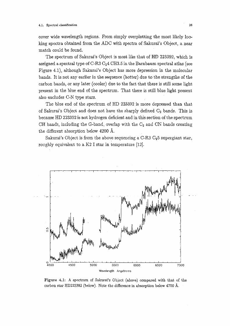
cover wide wavelength regions. From simply overplotting the most likely loaIcing spectra obtained from the ADO with spectra of Sakurai's Object, a near
match could be found. The spectrum of Sakurai's Object is most like that of HD 223392, which is
assigned a spectral type of O-R3 0 24 CH3.5 in the Barnbaum spectral atlas (see
Figure 4.1), although Sakurai's Object has more depression in the molecular
bands. It is not any earlier in the sequence (hotter) due to the strengths of the
carbon bands, or any later (cooler) due to the fact that there is still some light
present in the blue end of the spectrum. That there is still blue light present
also excludes C-N type stars.
The blue end of the spectrum of HD 223392 is more depressed than that
of Sakurai's Object and does not have the sharply defined 0 2 bands. This is
because HD 223392 is not hydrogen deficient and in this section of the spectrum
CH bands, including the G-band, overlap with the 0 2 and ON bands creating
the different absorption below 4200 A. Sakurai's Object is from the above sequencing a C-R3 C25 supergiant star,
roughly equivalent to a K2 I star in temperature (12}.
Wavelength Angstroms
Figure 4.1: A spectrum of Sakurai's Object (above) compared with that of the carbon star HD223392 (below). Note the difference in absorption below 4700 A.
4.2. Determination of bolometric magnitudes 27
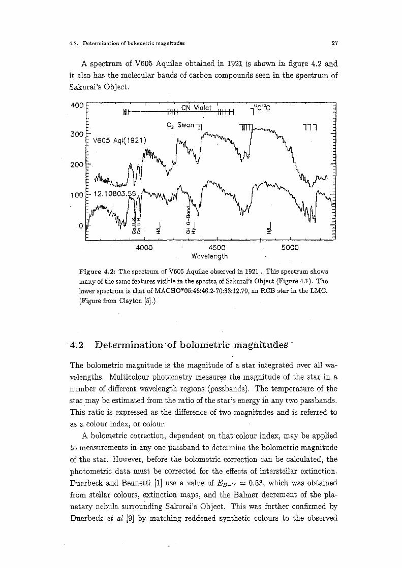
A spectrum of V605 Aquilae obtained in 1921 is shown in figure 4.2 and it also has the molecular bands of carbon compounds seen in the spectrum of Sakurai's Object.
400 Ill I Hill! CN Violet IIIII I
300
200
100
4000 4500 5000 Wavelength
Figure 4.2: The spectrum of V605 Aquilae observed in 1921 . This spectrum shows
many of the same features visible in the spectra of Sakurai's Object (Figure 4.1). The lower spectrum is that ofMACH0*05:46:46.2-70:38:12.79, an RCB star in the LMC.
(Figure from Clayton [5].) ·
· 4~2 Determination ·of bolometric magnituaes ~
The bolometric magnitude is the magnitude of a star integrated over all wavelengths. Multicolour photometry measures the magnitude of the star in a number of different wavelength regions (passbands). The temperature of the star may be estimated from the ratio of the star's energy in any two pass bands.
This ratio is expressed as the difference of two magnitudes and is referred to as a colour index, or colour.
A bolometric correction, dependent on that colour index, may be applied
to measurements in any one passband to determine the bolometric magnitude
of the star. However, before the bolometric correction can be calculated, the photometric data must be corrected for the effects of interstellar extinction.
Duerbeck and Bennetti [1] use a value of Es-v = 0.53, which was obtained from stellar colours, extinction maps, and the Balmer decrement of the planetary nebula surrounding Sakurai's Object. This was further confirmed by
Duerbeck et al [9] by matching reddened synthetic colours to the observed
4.2. Determination of bolometric magnitudes 28
photometry. Kimeswenger and Kerber [15] use EB-V = 0.54, but give no explanation of how that value was obtained.
Given EB-V it is possible to calculate extinctions for the other passbands,
for instance the extinction in the Cousins V passband is given by Av =
RvEB-V· The only problem is to obtain a suitable constant,(Rv), which is dependent on the passband itself and the nature of the interstellar absorbing
matter. Two ways of finding the bolometric correction have been used, one which
uses the ( B- V) colour index to give a correction based on the colours of normal
(not hydrogen deficient) stars, and another which uses the (R-I) colour index
to give a correction based on carbon stars in the Large Magellanic Cloud.
This means that corrections for the V, R and I pass bands were required.
Both Astrophysical Quantities [16] and Landolt and Bornstein[17] have similar
tables of wavelength versus extinction. The most widely accepted value for Rv
is 3.10 0.15 .
The response of the system used at MJUO is not entirely standard, espe
cially in the Rand I pass bands as a 820 photomultiplier tube is used instead
of the gallium arsenide tube prescribed in the Cousins UBVRI filter system
(see Bessell [7]). The photomultiplier tube used has a wavelength cutoff in
the I filter which effectively moves the peak of that filter function toward the
blue. The peaks of the filter functions for the R and I filters at MJUO are
R = 0.575,u and I = 0.750,u. Using these wavelengths to find the extinc
tions from the tabulated values in Astrophysical Quantities, ¥ = 0.93 and . v * =0.68. - Most of tlie variables used in this- analysis are not -well aenned. The peak
of the :flux through any filter is dependent on the colour of the star, and will
therefore probably have a different wavelength to the one tabulated.
First, using the (B- V) data and the bolometric corrections given for nor
mal supergiant stars in Astrophysical Quantities, Mbol was calculated for each individual data point and for the average data points used by Duerbeck et ar:.
The bolometric correction was chosen by spline interpolation of the values
given in Astrophysical Quantities [16], according to the (B- V) colour of the
star. It should be remembered that these figures are for late type normal stars,
presumably with oxide bands rather than carbon bands.
The second technique is a bolometric correction based on results from Costa
& Frogel [18], a study of 888 carbon stars in the LMC. This paper presents
RI and JKH photometry, and gives the following formula utilising (R-1) to
2In their analysis, Duerbeck et al used the average of measurements taken over a period of time, in order to negate the effect of any pulsations.
4.2. Determination of bolometric magnitudes 29
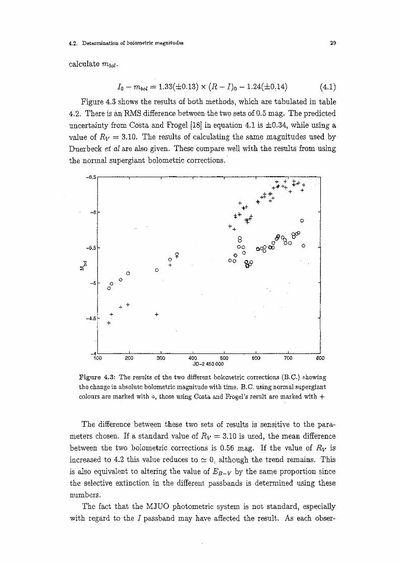
calculate mbol·
Io- mbol = 1.33(±0.13) X (R- I)o- 1.24(±0.14) (4.1)
Figure 4.3 shows the results of both methods, which are tabulated in table 4.2. There is an RMS difference between the two sets of 0.5 mag. The predicted
uncertainty from Costa and Frogel [18} in equation 4 .. 1 is ±0.34, while using a
value of Rv = 3.10. The results of calculating the same magnitudes used by Duerbeck et al are also given. These compare well with the results from using the normal supergiant bolometric corrections.·
-6.5.------r---....-------,;-------r---.----~----,
-6
-5.5
0 .0
:::E
-5 0
0 0
+
-4.5 +
+
0
+
0
+
0 ~ +
8 oo
0 0
oo ~
0
-4~--~---~--~~--~----~--~----~ 100 200 300 400 500 600 700 800
JD-2450000
Figure 4.3: The results of the two different bolometric corrections (B.C.) showing the change in absolute bolometric magnitude with time. B.C. using normal supergiant colours are marked with o, those using Costa and Frogel's result are marked with+
The difference between these two sets of results is sensitive to the para
meters chosen. If a standard value of Rv = 3.10 is used, the mean difference
between the two bolometric corrections is 0.56 mag. If the value of Rv is increased to 4.2 this value reduces to !::::! 0, although the trend remains. This
is also equivalent to altering the value of EB-V by the sam,e proportion since the selective extinction in the different passbands is determined using these
numbers. The fact that the MJUO photometric system is not standard, especially
with regard to the I passband may have affected the result. As each obser-
4.2. Determination of bolometric magnitudes 30
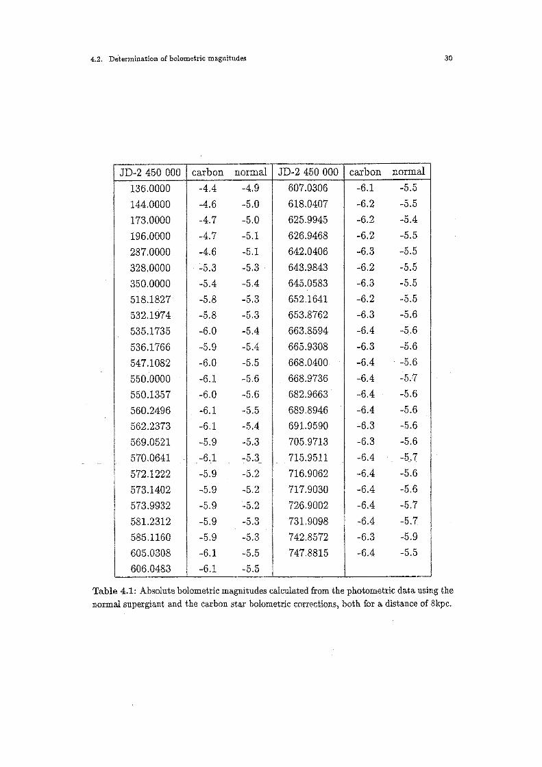
JD-2 450 000 carbon normal JD-2 450 000 carbon normal
136.0000 -4.4 -4.9 607.0306 -6.1 -5.5
144.0000 -4.6 -5.0 618.0407 -6.2 -5.5
173.0000 -4.7 -5.0 625.9945 -6.2 -5.4
196.0000 -4.7 -5.1 626.9468 -6.2 -5.5
287.0000 -4.6 -5.1 642.0406 -6.3 -5.5
328.0000 :.5.3 -5.3 643.9843 -6.2 -5.5
350.0000 -5.4 -5.4 645.0583 -6.3 -5.5
518.1827 -5.8 -5.3 652.1641 -6.2 -5.5
532.1974 -5.8 -5.3 653.8762 -6.3 -5.6
535.1735 -6.0 -5.4 663.8594 -6.4 -5.6
536.1766 -5.9 -5.4 665.9308 -6.3 -5.6
547.1082 -6.0 -5.5 668.0400 -6.4 -5.6
550.0000 -6.1 -5.6 668.9736 -6.4 -5.7
550.1357 -6.0 -5.6 682.9663 -6.4 -5.6
560.2496 -6.1 -5.5 689.8946 -6.4 -5.6
562.2373 -6.1 -5.4 691.9590 -6.3 -5.6
569.0521 -5.9 -5.3 705.9713 -6.3 -5.6
570.0641 -6.1 -5.3 715.9511 -6.4_ -5.7
572.1222 -5.9 -5.2 716.9062 -6.4 -5.6
573.1402 -5.9 -5.2 717.9030 -6.4 -5.6
573.9932 -5.9 -5.2 726.9002 -6.4 -5.7
581.2312 -5.9 -5.3 731.9098 -6.4 -5.7
585.1160 -5.9 -5.3 742.8572 -6.3 -5.9
605.0308 -6.1 -5.5 747.8815 -6.4 -5.5
606.0483 -6.1 -5.5
Table 4.1: Absolute bolometric magnitudes calculated from the photometric data using the normal supergiant and the carbon star bolometric corrections, both for a distance of 8kpc.
4.3. The distance to Sakurai's Object and the size of its planetary nebula. 31
vation is determined differentially with respect to standard stars, this will be
a problem if the energy distributions are different between the standard and
the observed stars. This is almost certainly the case. The magnitude of the
problem is difficult to estimate, given the unusual colour of Sakurai's Object
and the fact that no other differential I magnitudes have been published.
Duerbeck et al used the Bessell UBVR and Gunn i which means that their
i photometry data is incompatible with the bolometric correction from Costa
and Frogel. As these data were acquired in 1996.while the star was relatively hot and before it developed the molecular bands in its spectrum, the bolome
tric correction for normal supergiant stars is probably the best approximation
available.
In section 4.8 where these results have been compared to the available
models, the data from Duerbeck et al [9] have been corrected using the normal
supergiant bolometric correction, while for the MJUO photometry form 1997
after the molecular bands formed the bolometric corrections for C stars from
Costa and Frogel [18] have been used.
4.3 The distance to Sakurai's Object and the size of its planetary nebula.
There have been three estimates of the distance to Sakurai's Object. The first
was made by Duerbeck and Bennetti [1]. A statistical distance of 5.5 kpc was
found from the H (J :flux of the surrounding planetary nebula.
Duerbeck et al [9] make a second distance estimate based on the observed
line of sight velocity of Salmrai's Object (100km , which along with its
galactic co-ordinates, places it near the centre of the Galaxy, based on the work
of Pottasch [19] on the distribution of planetary nebulae . The galactic centre
is assumed to be 8 kpc away and the same distance is assumed for Sakurai's Object.
The third distance estimate, presented by Kimeswenger and Kerber [15]
is 1.1 kpc. This method uses the amount of interstellar reddening, and is
calibrated by making estimates of the absolute magnitude, the distance to and
the amount of reddening towards the stars in the direction of Sakurai's Object.
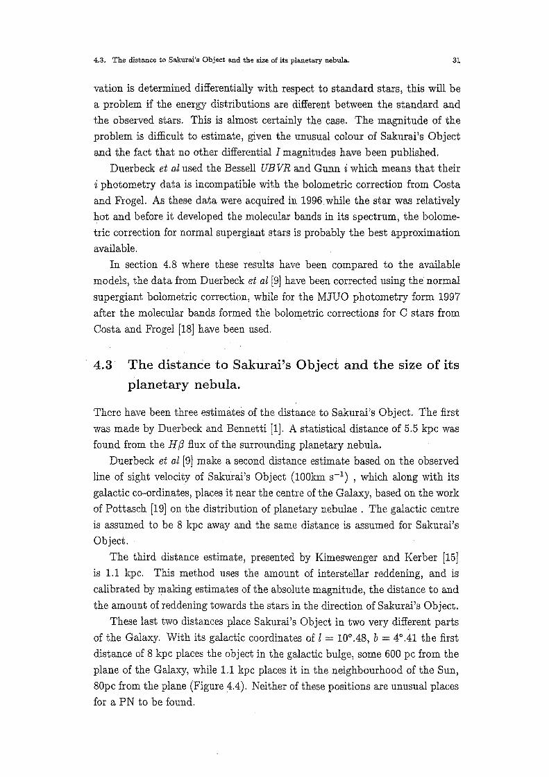
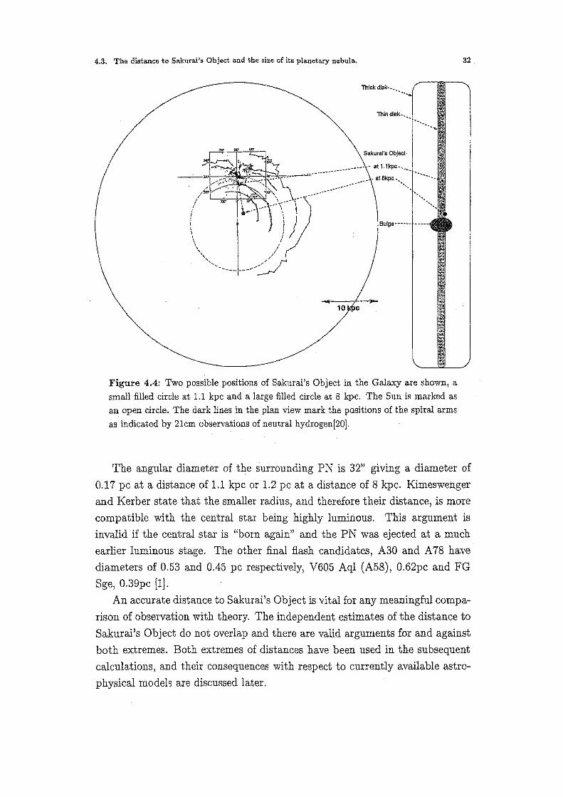
These last two distances place Sakurai's Object in two very different parts
of the Galaxy. With its galactic coordinates of l = 10°.48, b = 4°.41 the first
distance of 8 kpc places the object in the galactic bulge, some 600 pc from the
plane of the Galaxy, while 1.1 kpc places it in the neighbourhood of the Sun,
80pc from the plane (Figure 4.4). Neither of these positions are unusual places
for a PN to be found.
4.3. The distance to Sakurai's Object and the size of its planetary nebula.
~;--*-'w=~
Thick disk·
Thin
.................. • at 1.1kp<:· ••••
·~=----=_ .... -················· . at Skpo
Figure 4.4: Two possible positions of Sakurai's Ob)ect in the Galaxy are shown, a small filled circle at 1.1 kpc and a large filled circle at 8 kpc. The Sun is marked as an open circle. The dark lines in the plan view mark the positions of the spiral arms as indicated by 21cm observations of neutral hydrogen[20].
32
The angular diameter of the surrounding PN is 32" giving a diameter of
0.17 pc at a distance of 1.1 kpc or 1.2 pc at a distance of 8 kpc. Kimeswenger
and Kerber state that the smaller radius, and therefore their distance, is more
compatible with the central star being highly luminous. This argument is
invalid if the central star is "born again" and the PN was ejected at a much
earlier luminous stage. The other final flash candidates, A30 and A 78 have
diameters of 0.53 and 0.45 pc respectively, V605 Aql (A58), 0.62pc and FG
Sge, 0.39pc [lJ.
An accurate distance to Sakurai's Object is vital for any meaningful compa
rison of observation with theory. The independent estimates of the distance to
Sakurai's Object do not overlap and there are valid arguments for and against
both extremes. Both extremes of distances have been used in the subsequent
calculations, and their consequences with respect to currently available astro
physical models are discussed later.
4.4. The temperature of Sakurai's Object 33
4.4 The temperature of Sakurai's Object
Sakurai's Object is in the process of expanding and cooling. Duerbeck et al have derived temperatures by comparing the ( B- V) colour observed throughout
1996 to synthetic colours from model atmospheres of hydrogen-deficient carbon stars computed by Asplund et al [14].
For their photometric observations in early 1997 Duerbeck et al [9] give a
temperature of 6000 K. Their (B- V) values for early 1997 agree moderately
well with the values from MJUO, bearing in mind that each of their points
are the mean of a small number of observations. Unfortunately the three
measurements taken in 1997 are clustered around a localised maximum in the
light curve and are therefore not entirely representative of the time period (see
figure 2.4).
Using Asplund et al's synthetic colours for C star model atmospheres these
values indicate that Sakurai's Object has cooled from 6000 K to somewhere
around about 5000 K. Asplund's models only go down to 5000 K but he notes
in the text that the predictions tend to be 500 K hotter than the spectroscopic
evidence from real RCB stars would suggest. This is attributed to the models having too high a metallicity.
Using Duerbeck et al's colours and Asplund et al's model colour/temperature
estimates for the RCB stars, the temperatures found are about 100 degrees
higher than those reported by Duerbeck.
In a private communication Asplund has expressed some misgivings about
using his colours in this way, as the composition of Sakurai's Object differs
·from that used in the models. The models have a C/He ratio of 1% whereas
Sakurai's Object has a C/He of approximately 10%. This means that for a
given temperature, Asplund's models will be redder than SakuraPs Object, so
temperatures estimated from those models will tend to be too high. The model
temperatures, less 500 K, have been used as an upper limit for the temperature
of Sakurai's Object. New estimates will have to be made as better models become available.
4.5 The radius of Sakurai's Object
The radius of the star can be calculated using the following relationship.
(4.2)
or
4.6. Results 34
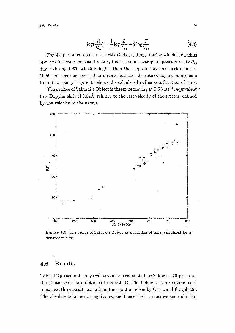
R 1 L T log(-)= -log-- 2log-~ 2 L0 T0
(4.3)
For the period covered by the MJUO observations, during which the radius appears to have increased linearly, this yields an average expansion of 0.3R0
day-1 during 1997, which is higher than that reported by Duerbeck et al for
1996, but consistent with their observation that the rate of expansion appears
to be increasing. Figure 4.5 shows the calculated radius as a function of time. The surface of Sakurai's Object is therefore moving at 2.6 kms-1, equivalent
to a Doppler shift of 0.04A relative to the rest velocity of the system, defined
by the velocity of the nebula.
~Or------.------,-~---.------,------,------.------,
+
200
150
100 +
+ +
50 + + +
0~----~------~----~------L-----~------L-----~ 100 200 300 400 500 600 700 800
JD-2 450 000
Figure 4.5: The radius of Sakurai's Object as a function of time, calculated for a distance of 8kpc.
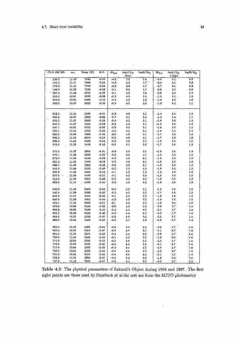
4.6 Results
Table 4.2 presents the physical parameters calculated for Sakurai's Object from
the photometric data obtained from MJUO. The bolometric corrections used
to correct these results come from the equation given by Costa and Frogel [18].
The absolute bolometric magnitudes, and hence the luminosities and radii that
4.7. Short term variability 35
have been calculated from them, using both 8kpc and 1.1kpc as the distance measurement.
Also included at the top of the table are the eight data points used by
Duerbeck et al [9] in their photometric analysis of Sakurai's Object. Each of
these eight points is the average of a number of observations over a short period
of time. For these points the bolometric correction for normal supergiant stars has been tabulated and the subsequent properties derived from that.
These results show a decrease in temperature and an increase in luminosity
and radius during 1996 and 1997. The luminosity has continued to increase
although the V magnitude peaked at some time during the seasonal break. The significance of these results with respect to the models of final flash objects is
discussed in section 4.8
4. 7 Short term variability
In addition to the overall increase in luminosity observed in Sakurai's Object,
there are variations in brightness on timescales shorter than 100 days. Photometry- from JD 2 450 136 to JD 2 450 556 has been published by
Duerbecket al [9]. Photometry also has been obtained at MJUO from JD 2 450 505 to JD 2 450 747. Both data sets are shown in figure 2.4 ..
Duerbeck et al find evidence for periodicities of 63, 25, 14 and 8 days
through Fourier analysis. By a different method applied to the residuals from
the 63-day curve, they find periods of 22.0, 13.8 and 7.7 days.
Multiple attempts at fitting the same data sets used by Duerbeck et al,
using the Lomb-Scargle Fourier analysis program T7 (see section 3.4) indicate
a period of between 58 and 72 days, and others of about 21, 13 and 7 days.
In the MJUO data set, a period of 60 days and an amplitude of 0.1 mag
was found using this Fourier Transform technique. No other periods could be
reliably identified. This may be because the data sampling is sparse or possibly
because, as the star becomes cooler, some modes are no longer unstable to pulsation. This is illustrated in figures 7 and 8 of Duerbeck et al [9]. The most
obvious thing about the light curve of SakuraPs Object during 1997 is that it varies over a much larger range, rv 0.5 magnitudes, compared to t'V 0.1 in 1996.
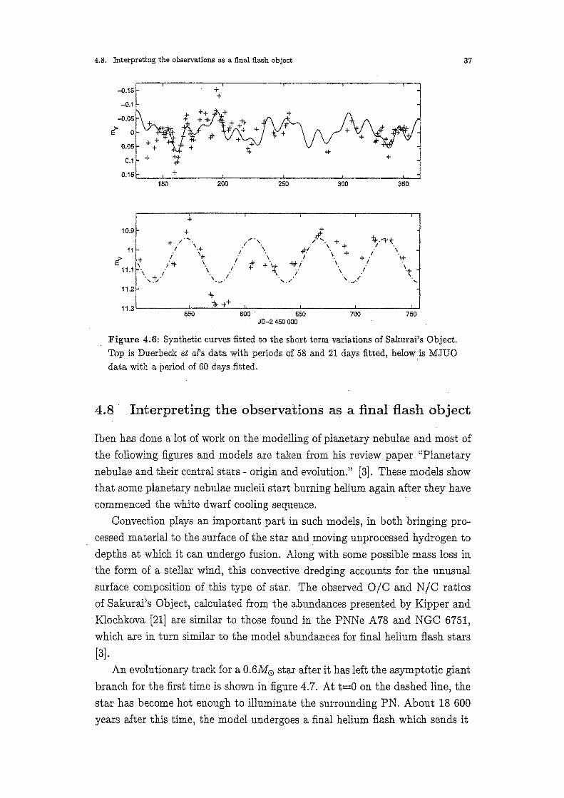
Figure 4.6 shows the data from Duerbeck et al with a synthetic curve
compounded from periods of 58 and 21 days. These data have had an overall
increasing trend removed (see section 3.4). The MJUO data, is shown in the
lower panel with a synthetic curve of 60 days.
4. 7. Short term variability 36
JD-2 450 000 mv Temp (K) B.C. Mbol logL/L0 logR./11.0 Mbol logL/L(iJ logR./11.0 8kpc l.lkpc
136.0 11.29 7550 -0.05 -4.9 3.8 1.6 -0.6 2.1 0.8 144.0 11.21 7400 -0.04 -4.9 3.8 1.7 -0.6 2.1 0.8 173.0 11.15 7350 -0.04 -5.0 3.9 L1 -0.7 2.1 0.8 196.0 11.05 7250 -0.03 -5.1 3.9 1.7 -0.8 2.2 0.9 287.0 11.03 6700 -0.05 -5.1 3.9 1.8 -0.8 2.2 0.9 328.0 10.91 6500 -0.08 -5.3 4.0 1.8 -1.0 2.2 1.0 350.0 10.85 6400 -0.10 -5.4 4.0 1.9 -1.0 2.3 1.0 550.0 10.87 5500 -0.30 -5.3 4.0 2.0 -1.0 2.2 1.1
518.2 11.14 5650 -0.61 -5.8 4.2 2.1 -1.4 2.4 1.2 532.2 10.97 6350 -0.68 -5.7 4.1 2.0 -1.4 2.4 1.1 535.2 11.07 5650 •0.56 -5.9 4.2 2.1 -1.6 2.5 1.2 536.2 11.07 5600 -0.58 -5.9 4.2 2.1 -1.6 2.5 1.2 547.1 10.91 5750 -0.65 -5.9 4.2 2.1 -1.6 2.5 1.2 550.1 10.84 5700 -0.66 -5.9 4.2 2.1 -1.6 2.5 1.2 560.2 10.99 5500 -0.56 -6.0 4.3 2.1 -1.7 2.5 1.3 562.2 11.03 5650 -0.54 -6.0 4.3 2.1 -1.7 2.5 1.3 569.0 11.22 5450 -0.54 -5.8 4.2 2.1 -1.5 2.5 1.2 570.0 11.23 5450 -0.43 -6.0 4.3 2.2 -1.7 2.5 1.3
572.1 11.27. 5500 -0.51 -5.8 4.2 2.1 -1.5 2.5 1.2 573.1 11.28 5500 -0.50 -5.8 4.2 2.1 -1.5 2.5 1.2 573.9 11.28 5450 -0.53 -5.8 4.2 2.1 -1.5 2.5 1.2 581.2 11.28 5400 -0.50 -5.9 4.2 2.1 -1.5 2.5 1.3 585.1 11.26 5350 -0.49 -5.9 4.2 2.1 -1.6 2.5 1.3 605.0 11.09 5350 -0.48 -6.1 4.3 2.2 -1.8 2.6 1.3 606.0 11.06 5400 -0.50 -6.1 4.3 2.2 -1.8 2.6 1.3 607.0 11.06 5450 -0.51 -6.1 4.3 2.2 -1.8 2.6 1.3 6],8.0 _ll.(l8 5350 -0.46 -6.2 4.3 2.2 -1.8 2.6 1.3 625.9 11.10 5400 -0.44 -6.2 4.3 2.2 -1.9 2.6 1.3
626.9 11.08 5300 -0.43 -6.2 4.3 2.2 -1.9 2.6 1.3 642.0 11.06 5350 -0.43 -6.2 4.3 2.2 -1.9 2.6 1.3 643.9 11.07 5350 -0.49 -6.1 4.3 2.2 -1.8 2.6 1.3 645.0 11.06 5350 -0.44 -6.2 4.3 2.2 -1.9 2.6 1.3 652.1 11.00 5500 -0.51 -6.1 4.3 2.2 -1.8 2.6 1.3 653.8 10.99 5350 -0.43 -6.3 4.4 2.2 -2.0 2.7 1.4 663.8 10.93 5400 -0.42 -6.4 4.4 2.2 -2.1 2.7 1.4 665.9 10.92 5400 -1>.46 -6.3 4.4 2.2 -2.0 2.7 1.4 668.0 10.91 5350 -0.47 -6.3 4.4 2.2 -2.0 2.7 1.4 668.9 10.89 5400 -0.47 -6.3 4.4 2.2 -2.0 2.7 1.4
682.9 10.95 5300 -0.44 -6.3 4.4 2.2 -2.0 2.7 1.4 689.8 10.97 5300 -0.37 -6.4 4.4 2.2 -2.1 2.7 1.4 691.9 11.01 5350 -0.42 -6.3 4.4 2.2 -2.0 2.7 1.4 705.9 11.04 5300 -0.44 -6.2 4.4 2.2 -1.9 2.6 1.4 715.9 10.98 5250 -0.45 -6.3 4.4 2.2 -2.0 2.1 1.4 116.9 10.95 5300 c0.40 -6.4 4.4 2.2 -2.1 2.7 1.4 717.9 10.94 5300 -0.45 -6.3 4.4 2.2 -2.0 2.7 1.4 726.9 10.94 5200 -0.44 -6.3 4.4 2.3 -2.0 2.7 1.4 731.9 10.94 5150 -0.44 -6.4 4.4 2.3 -2.1 2.7 1.4 742.8 11.04 4600 -0.45 -6.3 4.4 2.3 -1.9 2.6 1.5 747.8 11.10 5200 -0.37 -6.3 4.4 2.3 -2.0 2.7 1.4
Table 4.2: The physical parameters of Sakurai's Object during 1996 and 1997. The first eight points are those used by Duerbeck et al the rest are from the MJUO photometry
4.8. Interpreting the observations as a. fina.l fiash object
-0.15
-0.1
+ 10.9 + .,
+ / . 11 I '-+
> + I ':r E \ i+ \
11.1 \ . + .' ,,.,
11.2
11.3 550
+ +
' ·-"*f.
I
'4- ++
+ ,#:., + . \ +
.p;l \ + I
ill-."'f'-t I .
/ \ +/ "'!" -!;!-/ \ / 't
·' ...... ·' · ....
600 650 700 750 JD-2 450 000
Figure 4.6: Synthetic curves fitted to the short term variations of Sakurai's Object. Top is Duerbeck et afs data with periods of 58 and 21 days fitted, belowis MJUO data with a period of 60 days fitted.
37
4.8 · Interpreting the observations as a final flash object
Iben has done a lot of work on the modelling of planetary nebulae and most of
the following figures and models are taken from his review paper "Planetary
nebulae and their central stars- origin and evolution." [3]. These models show that some planetary nebulae nucleii start burning helium again after they have
commenced the white dwarf cooling sequence.
Convection plays an important part in such models, in both bringing pro
cessed material to the surface of the star and moving unprocessed hydrogen to
depths at which it can undergo fusion. Along with some possible mass loss in
the form of a stellar wind, this convective dredging accounts for the unusual
surface composition of this type of star. The observed 0/C and N/C ratios
of Sakurai's Object, calculated from the abundances presented by Kipper and
Klochkova [21] are similar to those found in the PNNe A 78 and NGC 6751,
which are in turn similar to the model abundances for final helium flash stars
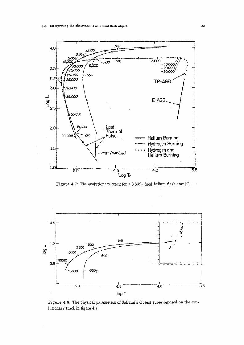
[3]. An evolutionary track for a 0.6M0 star after it has left the asymptotic giant
branch for the first time is shown in figure 4.7. At t=O on the dashed line, the
star has become hot enough to illuminate the surrounding PN. About 18 600
years after this time, the model undergoes a final helium flash which sends it
4.8. Interpreting the observations as a. final flash object
1=0
Last Thermal Pulse
E-AGB
Helium Burning Hydrogen Burning
• • • • Hydrogen and Helium Burning
l.OL-----=5=-'=.o=---.;._ ___ 4:~-:.5=-------.:4:~-::.oo-----~3.5
LogTe
Figure 4.7: The evolutionary track for a0.6M0 final helium flash star [2] .
5.0 4.5
logT
..
"
4.0
. . l
1\ ·t ... ;t
' .
Figure 4.8: The physical parameters of Sakurai's Object superimposed on the evolutionary track in figure 4. 7.
38
3.5
4.8. Interpreting the observations a.s a final flash object 39
back to a position of high luminosity and low temperature. It is believed to be during this rise back to the red giant phase that Sakurai's Object has been
discovered and observed.
The physical characteristics derived from the photometric observations of
Sakurai's Object, with an assumed distance of 8kpc, have been placed on
an enlarged portion of this diagram in figure 4.8. Bearing in mind that the
temperatures derived from Asplund's models are an upper limit, Sakurai's
Object is seen to be cooler and slightly more luminous than this particular
model predicts.
Especially interesting to note is the steep slope around the turnaround
point of the evolutionary track. This is not seen in the model, which may not
have been calculated on a fine enough time scale to predict such an event. This
can also be seen as evidence for the larger distance being more likely, as the
luminosities calculated for the shorter distance. ( ~ ~ 2.5) are too low to fit
any of Iben's models.
40
Chapter 5
Sakurai's Object in context
5.1 A comparison with other final flash objects
Sakurai's Object can now be placed in context with other suspected. final flash
· objects. These other objects may provide some idea as to what to expect in
the future.
5.1.1 The rise ...
Sakurai's Object has continued to increase in brightness since its discovery in early 1996. It has brightened by some 5 magnitudes in Vsince its discovery.
Of the other two possible final flash objects, this time scale is most similar to
V605 Aquilae, which increased by 5 magnitudes over a period of about two
years. By comparison, the other final flash object, FG Sagittae brightened by
I"J 4 magnitudes over a period of seventy years.
5.1.2 ... and fall of Sakurai's Object
As the luminosity of this object continued to increase until the end of the 1997
observing season this subsection may be a little premature. However, in 100%
of the cases so far, the carbon rich, hydrogen deficient final flash object has
produced an obscuring cloud of carbon dust at some stage in its evolution.
V605 Aquilae disappeared from sight some 7 years after its outburst in 1917 due to the formation of a thick cloud of dust. It still remains obscured. FG
Sagittae has recently started to show ROB-like declines.
Sakurai's Object may have already started to produce small amounts of dust, causing the short term fluctuations in brightness during 1997. No infra
red excess indicative of dust was observed by IRAS in 1983 (1}. It would be interesting to see if there was any infrared excess associated with the object
now. The models predict that a final flash object will increase in temperature at
near constant luminosity, over a timescale of"' 200 years.
5.2. Future observations 41
5.1.3 The surrounding nebulosity
The planetary nebulae surrounding final flash objects are large, with diameters
of about half a parsec. The nebula around Sakurai's Object, if a distance of
8kpc is assumed, has a diameter of 1.2pc, which is twice the size of A58,
the nebula around V605 Aquilae. This could indicate that 8kpc is too large a
distance. On the other hand, the alternate distance of 1.1kpc gives, along with
a much lower luminosity, a PN diameter of 0.17pc less than half the diameter
of the PN around FG Sagittae, which would seem to be too small.
Of the four final fl.ash objects, three of them (A30, A78 and V605 Aquilae) have knots of hydrogen deficient nebulosity associated with them. Evidence
of such a knot forming around Sakurai's Object should be looked for over the
next few decades.
5.1.4 The origin of the R Coronae Borealis stars
The final flash scenario is one of the possibilities suggested for the origin of the
dust producing RCB stars. Of the five (including Sakurai's Object) possible
FF candidates discussed four have definitely produced dust. Two (FG Sge and . V605 Aql) have undergone RCB like decline/recovery phases, although V605 ·
Aql has since disappeared inside a dust cloud. FG Sge has a similar spectral
type to other RCB stars. It appears that final flash objects may produce RCB
stars, but are more likely to vanish from sight completely in a cloud of dust.
Which path Sakurai's Object takes remains to be seen.
5.2 Future observations
Sakurai's Object appears to be evolving on a timescale similar to that of V605
Aquilae, which since its brightening in 1917 has developed molecular bands,
ejected a highly opaque dust cloud and more recently evolved toward hotter
temperatures ("'50 000 K). From this comparison it can be expected that Sakurai's Object has not yet finished its current stage of rapid morphological
change. Ongoing frequent photometric monitoring of Sakurai's Object should
therefore be maintained, for three reasons.
The short term variability of Sakurai's Object is not yet well defined and
may be evolving as the radius and temperature continue to change. If the
variability is the result of pulsations then this star might provide an instruc
tive example of variability at constant mass, but differing luminosities and
temperatures.
Dust production similar to that of the RCB stars may happen, or indeed
may have already happened in a small way. Both previous final flash objects,
5.3. Summary: Sakurai's Object in 1996 and 1997 42
V605 Aql and FG Sge have produced dust. V605 Aql disappeared from sight in 1923 after two RCB-like declines and has remained shrouded in dust ever
since. FG Sge, in line with its slower evolution, has only recently (1992) started
showing these RCB declines.
When observations ended in 1997 Sakurai's Object was still becoming coo
ler and brighter. According to the available models, this behaviour will stop and the star will become hotter again, while maintaining a constant lumino
sity. Determining the rate at which these changes take place can provide some observational constraints on the models and if Sakurai's Object continues to
evolve on a similar timescale to V605 Aql these changes can be expected to
happen in tens of years rather than tens of thousands of years.
It could also be useful to continue obtaining medium resolution spectra, when practical, perhaps as part of an RCB monitoring program, and also to
be able to obtain spectra at short notice if any profound photometric changes
are observed.
5.2.1 Dust
Early in 1997 the MJUO photometry shows a relatively large decline in brightness of f'..J 0.5 mag. This is much larger than the corresponding variations in
Duerbeck's data. Whether this variation is due to some internal change in the
pulsational characteristics of the star or the production of dust near the surface is undecided. There may be some possibility of investigating this problem
further through the use of two colour or colour-magnitude plots, but this is
further complicated by the fact that the star is intrinsically changing in co
lour. Some estimate of reddening, based on the star only and not that the
surrounding nebula and independent of the colour and composition of the star
is required. Infrared observation might also show evidence of dust.
5.3 Summary : Sakurai's Object in 1996 and 1997
Sakurai's Object has been observed throughout 1997, and similar observations
are available for 1996. During this time it decreased in temperature from
7800K to 5200K, and increased in luminosity by a factor of 4. The temperature
became low enough for a significant amount of carbon containing molecules
(C2 and CN) to form. The star's spectral type changed from a G supergiant
to a C-R3 supergiant.
If a distance of 8kpc is assumed, its luminosity has increased from logLL = 0
3.8 to 4.4. If the alternate distance of 1.1 kpc is used, then the luminosity has
changed from logLL = 2.1 to 2.7. The temperature and luminosity calculated 0

5.4. Postscript 43
for a distance of 8kpc locate Sakurai's Object at the coolest extent of the final flash evolutionary track for a 0.6 M0 planetary nebula nucleus [3). This is
evidence for this object being located closer to 8kpc than 1.1 kpc. However, the relationship between the temperature and luminosity of the object increases rather more steeply than Iben's model would predict.
The change in temperature and luminosity is consistent with the object expanding from 40R0 to 200R0 . The rate of the expansion appears to have
increased over this time, from "" 0.1R0 day-1 to "" 0.3R0 day-1.
At the end ofthe 1997 observing season Sakurai's Object was still increasing
in luminosity. It is expected that eventually this increase will cease and the object will evolve at constant luminosity back to higher temperatures.
5.4 Postscript
Sakurai's Object is fading as predicted. This IAU circular dated 1998 Febr.uary 19 has recently been received by e-mail from Asplund announcing the first
visual decline of Sakurai's Object.
1998 February 19 (6824)
Central Bureau for Astronomical Telegrams INTERNATIONAL ASTRONOMICAL UNION
Daniel W. E. Gree
Circular No. 6825
Mailstop 18, Smith~onian Astrophysical Observatory, Cambridge, MA 02138, U.S.A. [email protected] or FAX 617-495-7231 (subscriptions) [email protected] or [email protected] (science)
URL http://cfa-www.harvard.edu/iau/cbat.html Phone 617-495-7244/7440/7444 (for emergency use only)
V4334 SAGITTARII
W. Liller, Institute Isaac Newton, Vina del Mar, Chile; M.
Janson, Groningen University; H. W. Duerbeck, Muenster University; and A. van Genderen, Leiden University, report that this object (cj
IAUC 6718) has faded by almost 2 mag since last November, indicatii that the predicted dust formation (Duerbeck et al. 1997, A.J. 114, 1657) from the presumed final helium flash has begun. During 1997
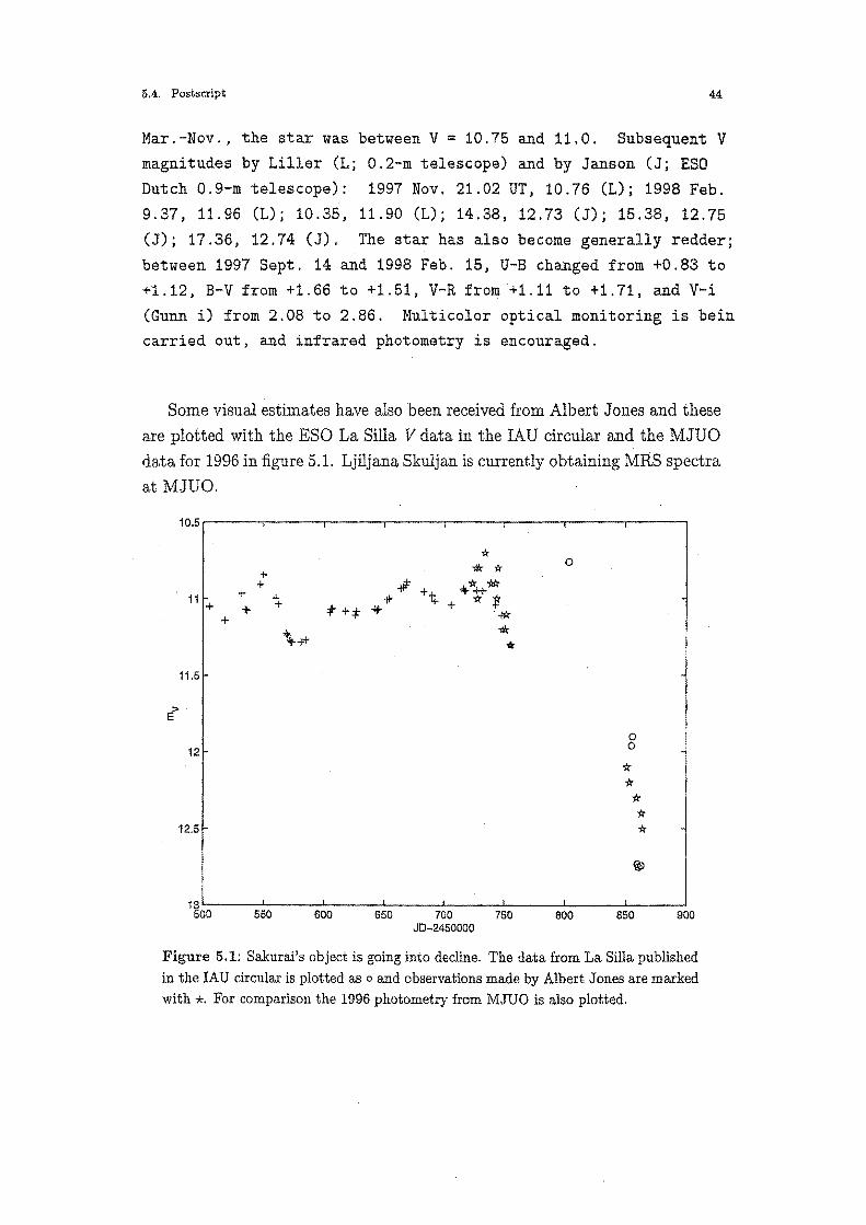
5.4. Postscript 44
Mar.-Nov., the star was between V = 10.75 and 11.0. Subsequent V magnitudes by Liller (L; 0.2-m telescope) and by Janson (J; ESO
Dutch 0.9-m telescope): 1997 Nov. 21.02 UT, 10.76 (L); 1998 Feb.
9.37, 11.96 (L); 10.35, 11.90 (L); 14.38, 12.73 (J); 15.38, 12.75
(J); 17.36, 12.74 (J). The star has also become generally redder; between 1997 Sept. 14 and 1998 Feb. 15, U-B changed from +0.83 to +1.12, B-V from +1.66 to +1.51, V-R from +1.11 to +1.71, and V-i
(Gunn i) from 2.08 to 2.86. Multicolor optical monitoring is bein carried out, and infrared photometry is encouraged.
Some visual estimates have also been received from Albert Jones and these
are plotted with the ESO La Silla V data in the IAU circular and the MJUO
data for 1996 in figure 5.1. Ljiljana Skuljan is currently obtaining MRS spectra
at MJUO.
10.5 r---.,----..,-----.---.----,----.,---,------,
11 +
11.5
12
12.5
+
+ +
+ +
* 1k *
J: ~* '#< -1+' +it- + r- $'
t +;f .;;. '*
0
0 0
* * * * *
13~--~--~---~---L--~--~~---~-~ 500 550 600 650 700 750 800 850 900
JD-2450000
Figure 5.1: Sakurai's object is going into decline. The data from La Silla published in the IAU circular is plotted as o and observations made by Albert Jones are marked with *· For comparison the 1996 photometry from MJUO is also plotted.

45
Chapter 6
Acknowledgements
I would like to thank Peter Cottrell for offering me this project and for his
advice and cheerful encouragement throughout the year. I would also like to thank Florian Kerber for bringing this once in a lifetime object to our attention.
This project would not have happened without the help of the technical staff at MJUO, especially Alan Gilmore and Pam Kilmartin who obtained the
photometric data used in this study. I would also like to thank Alan and Pam
for some excellent dinners and company while I was observing at Mount John.
I would also like to thank the other members of the astronomy group for their freely given support and advice, especially Ljiljana Skuljan who taught
me how to use the MRS and also obtained some observations of Sakurai's
Object while on her observing runs. Other people who provided valuable information were Albert Jones with
his visual estimates of the magnitude of Sakurai's Object and Martin Asplund with his colours from model C stars.
This piece of res·earch has also made use of the Simbad database, operated at
CDS Strasbourg, France, and the Astronomical Data center and Astrophysics
Data System abstract service, both provided by NASA. All of these databases were accessed via the World Wide Web.
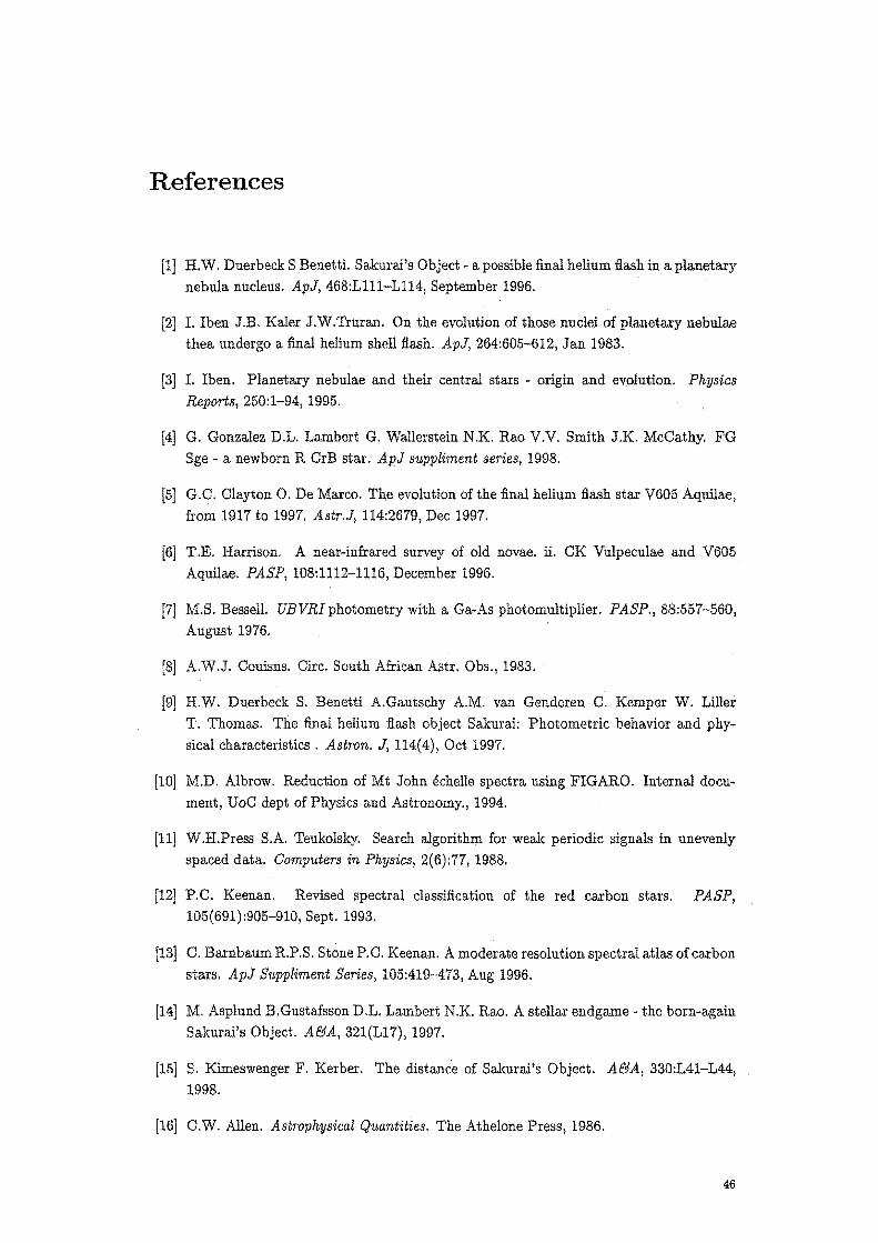
References
(1] H.W. Duerbeck S Benetti. Sakurai's Object~ a possible final helium flash in a planetary nebula nucleus. ApJ, 468:L111-Ll14, September 1996.
(2] L Iben J.B. Kaler J.W.Truran. On the evolution of those nuclei of planetary nebulae thea undergo a final helium shell flash. ApJ, 264:605-612, Jan 1983.
[3] I. Iben. Planetary nebulae and their central stars - origin and evolution. Physics
Reports, 250:1-94, 1995.
[4] G. Gonzalez D.L. Lambert G. Wallerstein N.K. Rao V.V. Smith J.K. McCathy. FG Sge ~ a newborn R CrB star. ApJ suppliment series, 1998.
[5] G.C. Clayton 0. De Marco. The evolution of the :final helium flash star V605 Aquilae, from 1917 to 1997. Astr.J, 114:2679, Dec 1997.
[6] T.E. Harrison. A near~infrared survey of old novae. ii. CK Vulpeculae and V605 Aquilae. PASP, 108:1112-1116, December 1996.
(7] M.S. Bessell. UBVRiphotometry with a Ga-As photomultiplier. PASP., 88:557-560, August 1976.
[8] A.W.J. Couisns. Circ. South African Astr. Obs., 1983.
[9] H.W. Duerbeck S. Benetti A.Gautschy A.M. van Genderen C. Kemper W. Liller T. Thomas. The final helium flash object Sakurai: Photometric behavior and phy~ sical characteristics. Astron. J, 114(4), Oct 1997.
(10] M.D. Albrow. Reduction of Mt John echelle spectra using FIGARO. Internal document, UoC dept of Physics and Astronomy., 1994.
[11] W.H.Press S.A. Teukolsky. Search algorithm for weak periodic signals in unevenly spaced data. Computers in Physics, 2(6):77, 1988.
[12) P.C. Keenan. Revised spectral classification of the red carbon stars. PASP, 105(691):905-910, Sept. 1993.
[13] C. Barnbaum R.P.S. Stone P.C. Keenan. A moderate resolution spectral atlas of carbon stars. ApJ Suppliment Series, 105:419-473, Aug 1996.
[14] M. Asplund B.Gustafsson D.L. Lambert N.K. Rao. A stellar endgame~ the born-again Sakurai's Object. A&A, 32l(L17), 1997.
[15] S. Kimeswenger F. Kerber. The distanc'e of Sakurai's Object. A&A, 330:L41-L44, 1998.
[16] C.W. Allen. Astrophysical Quantities. The Athelone Press, 1986.
46
References 47
[17] Landolt-Bornstein. New Series.
[18] E Costa J.A. Frogel. Carbon stars in the Large Magellanic cloud: Luminosities, colours
and implications for the history of star formation. Astron. J, 112(6), Dec 1996.
[19} S.R. Pottasch. Planetary Nebulae. Reidel, Dordrecht, 1984.
[20} M. Zeilek E.v.P. Smith. Introductory astronomy and astrophysics. Saunders College
Publishing, second edition, 1987.
[21] T. Kipper V.G. Klochkova. The chemical composition of Sakurai's Object. A&A,
324:L65-L68, 1997.
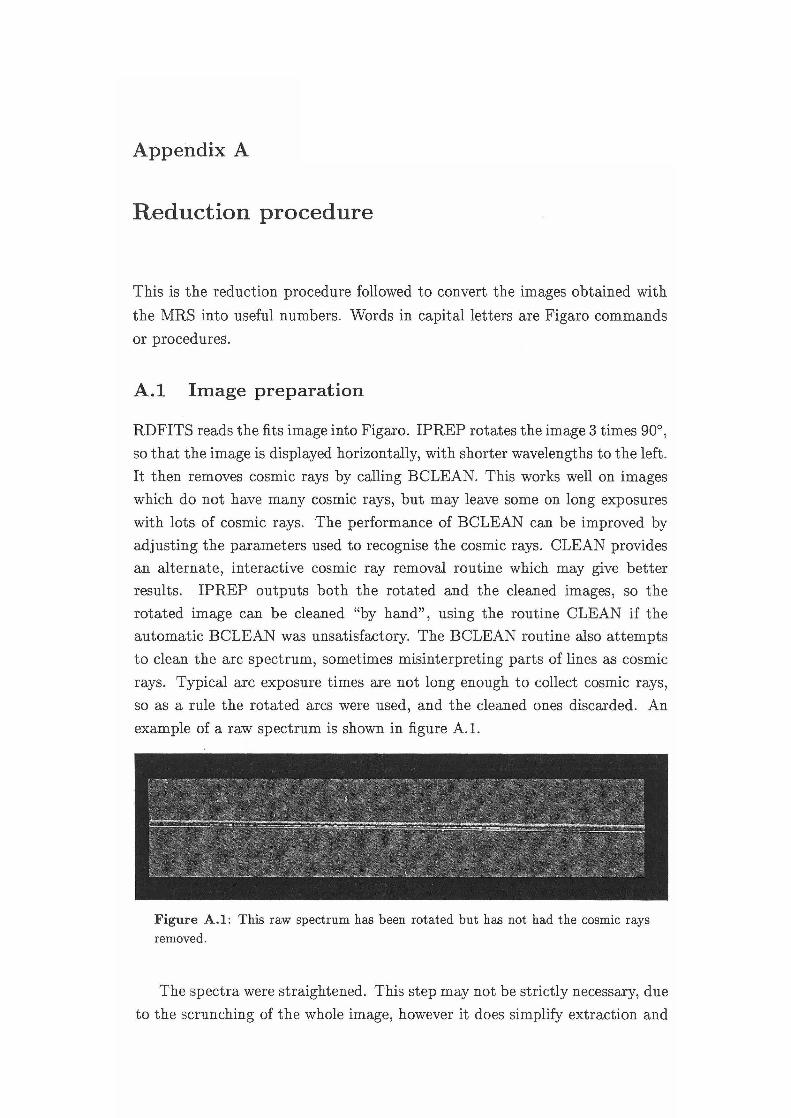
Appendix A
Reduction procedure
This is the reduction procedure followed to convert the images obtained with
the MRS into useful numbers. Words in capital letters are Figaro commands
or procedures.
A.l Image preparation
RDFITS reads the fits image into Figaro. IPREP rotates the image 3 times 90° ,
so that the image is displayed horizontally, with shorter wavelengths to the left.
It then removes cosmic rays by calling BCLEAN. This works well on images
which do not have many cosmic rays, but may leave some on long exposures
with lots of cosmic rays. The performance of BCLEAN can be improved by
adjusting the parameters used to recognise the cosmic rays. CLEAN provides
an alternate, interactive cosmic ray removal routine which may give better
results. IPREP outputs both the rotated and the cleaned images, so the
rotated image can be cleaned "by hand", using the routine CLEAN if the
automatic BCLEAN was unsatisfactory. The BCLEAN routine also attempts
to clean the arc spectrum, sometimes misinterpreting parts of lines as cosmic
rays . Typical arc exposure times are not long enough to collect cosmic rays,
so as a rule the rotated arcs were used, and the cleaned ones discarded. An
example of a raw spectrum is shown in figure A.l.
Figure A.l: This raw spectrum has been rotated but has not had the cosmic rays removed .
The spectra were straightened. This step may not be strictly necessary, due
to the scrunching of the whole image, however it does simplify extraction and
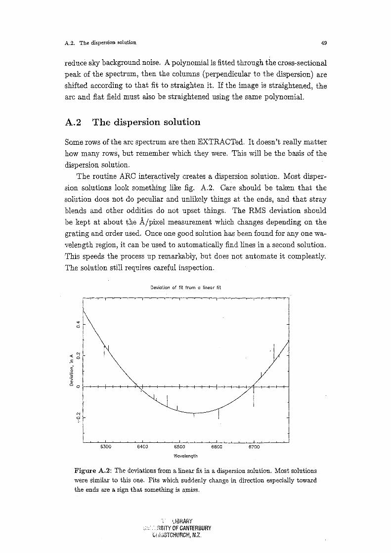
A.2. The dispersion solution 49
reduce sky background noise. A polynomial is fitted through the cross-sectional peak of the spectrum, then the columns (perpendicular to the dispersion) are shifted according to that fit to straighten it. If the image is straightened, the arc and :fiat :field must also be straightened using the same polynomiaL
A.2 The dispersion solution
Some rows of the arc spectrum are then EXTRACTed. It doesn't really matter how many rows, but remember which they were. This will be the basis of the
dispersion solution.
The routine ARC inte~actively creates a dispersion solution. Most dispersion solutions look something like fig. A.2. Care should be taken that the solution does not do peculiar and unlikely things at the ends, and that stray
blends and other oddities do not upset things. The RMS deviation should
be kept at about the A/pixel measurement which changes depending on the grating and order used. Once one good solution has been found for any one wavelength region, it can be used to automatically find lines in a second solution. This speeds the process up remarkably, but does not automate it compleatly.
The solution still requires careful inspection.
N d I
6300 6400
Deviation of fit from a linear fit
6500 6600 6700
Wavelength
Figure A.2: The deviations from a linear fit in a dispersion solution. Most solutions were similar to this one. Fits which suddenly change in direction especially toward the ends are a sign that something is amiss.
i.I8RARY ,:::· ·~.HSITY OF CANTERBURY
Gi :iiiSTCHURCH, N.Z.

A.3. Scrunching 50
A.3 Scrunching
Scrunching is the term applied to using the dispersion solution to assign wa
velength values to the image of the stellar spectrum.
IARC extends the dispersion solution over the entire arc image, assigning
each pixel in the arc spectrum a wavelength value, taking into account shifts
between rows. This is then used to assign wavelength values to the indivi
dual pixels in the image with !SCRUNCH. This step can obviate the need for
straightening the image, since each pixel is assigned a wavelength rather than
each column. If the unstraightened spectrum is prepared like this and then
all the rows containing stellar spectrum extracted, more sky is included than
is strictly necessary. The arc spectrum should be !SCRUNCHed, and then
inspected for any discontinuities on lines or other odd-looking bits. These can
usually be dealt with by varying the prompted parameters when using IARC.
Problems well away from the central few rows can be tolerated, as that part
of the image is not going to be used, but these regions should be noted and
avoided when choosing regions of the image for sky subtraction (see figure A.3.
Figure A.3: This scrunched arc spectrum is an indication of an acceptable IARC.
The slight deviations at the ends of the more intense lines are all right because they
are well away from the part of the spectrum that will be extracted.
A.4 Sky subtraction
The part of the !SCRUNCHed image with the spectrum in it is extracted,
usually about 10 rows. Sky subtraction can be done now if necessary. For
sky subtraction 10 rows are extracred from the !SCRUNCHed image, away
from the stellar spectrum and from any parts which exhibited problems after
!SCRUNCHing the arc. If there is serious noise or cosmic rays in this image,
repeat 3 times, and use the MEDIAN command, which takes the point by
point median of three files. This can also deal with cosmic rays which have
not been removed previously. This 1D sky spectrum is subtracted from the
1D stellar spectrum.

A.4. Sky subtraction 51
The result of these procedures is a one-dimensional wavelength calibrated spectrum, with sky lines subtracted. The fitting of a continuum to this spectrum is complicated by the type of star that has been observed, and is discussed in Chapter 3.
Recommended