0
R/V Mirai Cruise Report
MR15-05
WOCE-revisit in the eastern Indian Ocean
23rd December 2015 – 25th January 2016
Japan Agency for Marine-Earth Science and Technology
(JAMSTEC)

Cruise Report ERRATA of the Nutrients part
page Error Correction
97 potassium nitrate
CAS No. 7757-91-1
potassium nitrate
CAS No. 7757-79-1
94 1N H2SO4 1M H2SO4

Content
I. Introduction
II. Observation
1. Cruise Information 2. Underway Measurements
2.1 Navigation
2.2 Swath Bathymetry
2.3 Surface Meteorological Observation
2.4 Thermo-Salinograph and Related Measurements
2.5 Surface pCO2
2.6 Ceilometer
2.7 Surface CO2 fluxes
2.8 Radars and Disdrometers
2.9 Aerosol optical characteristics measured by Ship-borne Sky radiometer
2.10 Aerosol and gases
2.11 Sea surface gravity
2.12 Sea Surface Magnetic Field
2.13 Satellite image acquisition
3. Station Observation 3.1 CTDO2 Measurements
3.2 Bottle Salinity
3.3 Density
3.4 Oxygen
3.5 Nutrients
3.6 Chlorofluorocarbons and Sulfur hexafluoride
3.7 Carbon items
3.8 Calcium and Total alkalinity 2
3.9 Dissolved organic carbon and total dissolved nitrogen
3.10 Chlorophyll a
3.11 Absorption coefficients of particulate matter and colored dissolved organic matter (CDOM)
3.12 Bio-sampling
3.13 Carbon isotopes

--
2
3.14 Radioactive Cesium
3.15 Stable Isotopes of Water
3.16 Primary productivity
3.17 Lowered Acoustic Doppler Current Profiler
3.18 XCTD
3.19 Micro Rider
4. Floats, Drifters and Moorings 4.1 Argo floats
III. Notice on Using

--
3
I. Introduction
Indonesian Throughflow is a surface component of the global ocean circulation, which transports fresh Pacific
upper water masses into the north Indian Ocean with strong modification from the air-sea interaction and tidal
mixing. Paucity of observation data in this part of the world ocean has always been a restriction in understanding
global climate change and air-sea coupling — a problem shared amongst emerging international programmes such
as Eastern Indian Ocean Upwelling Research Initiative. The main purpose of this cruise is to measure the
distribution of water properties (temperature, salinity, dissolved oxygen, carbon, nutrients, etc.) in this important
ocean. This is a contribution to International Indian Ocean Expedition 2 and conducted under the Global Ocean
Ship-based Hydrographic Investigation Programme (GO-SHIP http://www.go-ship.org).
II. Observation

--
4
1. Cruise Information
Katsuro Katsumata (JAMSTEC)
Akihiko Murata (JAMSTEC)
1.1. Basic Information
Title of the cruise Research cruise on ocean decadal variability -- Indian Ocean GO-SHIP (Global Ocean
Ship-based Hydrographic Investigation Program)
Cruise track: See Fig. 1.1.1
Research area The northeastern Indian Ocean and the western Pacific Ocean
Cruise code: MR15-05
Expocode Leg 1: 49NZ20151223
Leg 2: 49NZ20160113
GHPO section designation: I10
Ship name: R/V Mirai
Ports of call: Leg 1, Jakarta, Indonesia – Bali, Indonesia
Leg 2, Bali, Indonesia – Yokohama, Japan
Cruise date: Leg 1, 23 December 2015 – 11 January 2016
Leg 2, 13 January 2016 – 25 January 2016
Chief scientists: Leg 1, Katsuro Katsumata ([email protected])
Leg 2, Akihiko Murata ([email protected])
Ocean Climate Change Research Program
Research and Development Centre for Global Change (RIGC)
Japan Agency for Marine-Earth Science and Technology (JAMSTEC)
2-15 Natsushima, Yokosuka, Kanagawa, Japan 237-0061
Fax: +81-46-867-9835

--
5
Piggyback projects
(1) Aerosol optical characteristics measured by ship-borne Sky radiometer (Toyama University)
(2) Geochemical and microbiological investigation from sea surface to sea bottom at tropical eutrophic ocean
(JAMSTEC, University of Tokyo, Tokyo University of Agriculture and Technology, Rakuno Gakuen University,
etc.)
(3) Advanced measurements of aerosols in the marine atmosphere: Toward elucidation of interactions with climate
and ecosystem (JAMSTEC)
(4) Global distribution of drop size distribution of precipitating particles over pure-oceanic background
(JAMSTEC)
(5) Shipboard CO2 observations over the tropical Indo-Pacific Ocean for a simple estimation of the carbon flux
between the ocean and the atmosphere from GOSAT data (JAXA)
Principal investigators of the piggyback projects: Kazuma Aoki (University of Toyama)
Takuro Nunoura (JAMSTEC)
Yugo Kanaya (JAMSTEC)
Masaki Katsumata (JAMSTEC)
Kei Shiomi (JAXA)
Number of Stations: Leg 1, 53 stations
Leg 2, none
Floats and drifters deployed: 16 Argo floats (Leg 1), 1 Argo float (Leg 2)
Mooring recovery : none

--
6
Fig. 1.1.1 MR15-05 cruise. Blue circles show the deployment position of Argo floats. Red dots show CTD/bottle
sampling stations.

--
7
Fig. 1.1.2 Water sampling positions.
1.2. Cruise Participants
List of Participants for leg 1
Katsuro Katsumata Chief scientist RCGC/JAMSTEC
Yuichiro Kumamoto DO/Sampling chief RCGC/JAMSTEC
Hiroshi Uchida Thermosalinograph/Salinity RCGC/JAMSTEC
Ken’ichi Sasaki CFCs MIO/JAMSTEC
Kosei Sasaoka Chlorophyll RCGC/JAMSTEC
Etsuro Ono Calcium/total alkalinity RCGC/JAMSTEC
Kazuhiko Matsumoto Primary productivity DEGCR/JAMSTEC
Taichi Yokokawa Biological sampling RDCMB/JAMSTEC
Chisato Yoshikawa Biological sampling DB/JAMSTEC
Shotoku Kotajima Biological sampling TUAC
Kanta Chida Biological sampling Rakuno Gakuen University

--
8
Harun Idham Akbar Water sampling BPPT
Gentio Harusono Security Officer Indonesian Navy
Hiroshi Matsumaga Chief technician/Sampling chief MWJ
Shinsuke Toyoda CTD MWJ
Hiroki Ushiromura Salinity MWJ
Syungo Oshitani CTD MWJ
Sonoka Wakatsuki Salinity MWJ
Keisuke Takeda CTD MWJ
Minoru Kamata Nutrients MWJ
Tomonori Watai pH/total alkalinity MWJ
Makoto Takada DIC MWJ
Elena Hayashi Nutrients MWJ
Atsushi Ono DIC MWJ
Tomomi Sone Nutrients MWJ
Katsunori Sagishima CFCs MWJ
Hironori Sato CFCs MWJ
Misato Kuwahara DO MWJ
Masahiro Orui DO MWJ
Keitaro Matsumoto DO MWJ
Hiroshi Hoshino CFCs MWJ
Haruka Tamada DO MWJ
Hiroyuki Hayashi CTD MWJ
Kanako Yoshida pH/total alkalinity MWJ
Kohei Miura Nutrients MWJ
Seika Katayama Water sampling MWJ
Naoya Yokoi Water sampling MWJ
Kohei Kumagai Water sampling MWJ
Naoya Kudo Water sampling MWJ
Eri Yoshizawa Water sampling MWJ
Kei Takamiya Water sampling MWJ
Wataru Tokunaga Chief technician/meterology/geophysics/XCTD GODI
Yutaro Murakami Meteorlology/geophysics/XCTD GODI
Tetsuya Kai Meteorology/geophysics/XCTD GODI
--
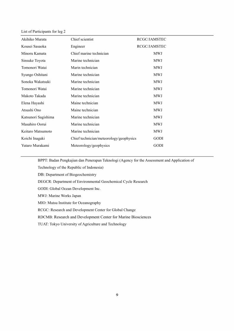
9
List of Participants for leg 2
Akihiko Murata Chief scientist RCGC/JAMSTEC
Kousei Sasaoka Engineer RCGC/JAMSTEC
Minoru Kamata Chief marine technician MWJ
Sinsuke Toyota Marine technician MWJ
Tomonori Watai Marin technician MWJ
Syungo Oshitani Marine technician MWJ
Sonoka Wakatsuki Marine technician MWJ
Tomonori Watai Marine technician MWJ
Makoto Takada Marine technician MWJ
Elena Hayashi Maine technician MWJ
Atsushi Ono Maine technician MWJ
Katsunori Sagishima Marine technician MWJ
Masahiro Oorui Marine technician MWJ
Keitaro Matsumoto Marine technician MWJ
Koichi Inagaki Chief technician/meteorology/geophysics GODI
Yutaro Murakami Meteorology/geophysics GODI
BPPT: Badan Pengkajian dan Penerapan Teknologi (Agency for the Assessment and Application of
Technology of the Republic of Indonesia)
DB: Department of Biogeochemistry
DEGCR: Department of Environmental Geochemical Cycle Research
GODI: Global Ocean Development Inc.
MWJ: Marine Works Japan
MIO: Mutsu Institute for Oceanography
RCGC: Research and Development Center for Global Change
RDCMB: Research and Development Center for Marine Biosciences
TUAT: Tokyo University of Agriculture and Technology

2. Underway Measurements 2.1 Navigation (1) Personnel
Katsuro Katsumata JAMSTEC: Principal investigator - leg1 - Akihiko Murata JAMSTEC: Principal investigator - leg2 - Wataru Tokunaga Global Ocean Development Inc., (GODI) - leg1 - Tetsuya Kai GODI - leg1 - Koichi Inagaki GODI - leg2 - Yutaro Murakami GODI - leg1, leg2 - Ryo Kimura MIRAI crew - leg1 - Masanori Murakami MIRAI crew - leg2 -
(2) System description
Ship’s position and velocity were provided by Navigation System on R/V MIRAI. This system integrates GNSS position, Doppler sonar log speed, Gyro compass heading and other basic data for navigation. This system also distributed ship’s standard time synchronized to GPS time server via Network Time Protocol. These data were logged on the network server as “SOJ” data every 5 seconds. Sensors for navigation data are listed below;
i) GNSS system:
R/V MIRAI has four GNSS systems, all GNSS positions were offset to radar-mast position, datum point. Anytime changeable manually switched as to GNSS receiving state. a) StarPack-D (version 1), Differential GNSS system.
Antenna: Located on compass deck, starboard. b) StarPack-D (version 1), Differential GNSS system.
Antenna: Located on compass deck, portside. c) Standalone GPS system.
Receiver: Trimble SPS751 Antenna: Located on navigation deck, starboard.
d) Standalone GPS system. Receiver: Trimble SPS751 Antenna: Located on navigation deck, portside.
ii) Doppler sonar log: FURUNO DS-30, which use three acoustic beam for current measurement under the hull.
iii) Gyro compass: TOKYO KEIKI TG-6000, sperry type mechanical gyrocompass.
iv) GPS time server: SEIKO TS-2540 Time Server, synchronizing to GPS satellites every 1 second.
(3) Cruise period (Times in UTC)
Leg1: 03:10, 23 Dec. 2015 to 00:50, 11 Jan. 2016 Leg2: 01:00, 13 Jan. 2016 to 23:50, 24 Jan. 2016

--
11
Fig.2.1-1 Cruise track of MR15-05Leg1, Leg2

--
12
2.2 Swath Bathymetry (1) Personnel
Katsuro Katsumata JAMSTEC: Principal investigator - leg1 - Akihiko Murata JAMSTEC: Principal investigator - leg2 - Wataru Tokunaga Global Ocean Development Inc., (GODI) - leg1 - Tetsuya Kai GODI - leg1 - Koichi Inagaki GODI - leg2 - Yutaro Murakami GODI - leg1, leg2 - Ryo Kimura MIRAI crew - leg1 - Masanori Murakami MIRAI crew - leg2 -
(2) Introduction
R/V MIRAI is equipped with a Multi narrow Beam Echo Sounding system (MBES), SEABEAM 3012 (L3 Communications, ELAC Nautik). The objective of MBES is collecting continuous bathymetric data along ship’s track to make a contribution to geological and geophysical investigations and global datasets.
(3) Data Acquisition
The “SEABEAM 3012” on R/V MIRAI was used for bathymetry mapping during this cruise. To get accurate sound velocity of water column for ray-path correction of acoustic multibeam, we used
Surface Sound Velocimeter (SSV) data to get the sea surface sound velocity (at 6.62m), and the deeper depth sound velocity profiles were calculated by temperature and salinity profiles from CTD and XCTD data by the equation in Del Grosso (1974) during this cruise.
Table 2.2-1 shows system configuration and performance of SEABEAM 3012.
Table 2.2-1 SEABEAM 3012 system configuration and performance ---------------------------------------------------------------------------------------------------------------------- Frequency: 12 kHz Transmit beam width: 2.0 degree Transmit power: 4 kW Transmit pulse length: 2 to 20 msec. Receive beam width: 1.6 degree Depth range: 50 to 11,000 m Number of beams: 301 beams Beam spacing: Equi-angle Swath width: 60 to 150 degrees Depth accuracy: < 1 % of water depth (average across the swath)
(4) Data processing
i) Sound velocity correction Each bathymetry data were corrected with sound velocity profiles calculated from the nearest CTD or
XCTD data in the distance. The equation of Del Grosso (1974) was used for calculating sound velocity. The data correction were carried out using the HIPS software version 8.1.8 (CARIS, Canada)
ii) Editing and Gridding Editing for the bathymetry data were carried out using the HIPS. Firstly, the bathymetry data during
ship’s turning was basically deleted, and spike noise of each swath data was removed. Then the bathymetry data were checked by “BASE surface (resolution: 50 m averaged grid)”.
Finally, all accepted data were exported as XYZ ASCII data (longitude [degree], latitude [degree], depth [m]), and converted to 150 m grid data using “nearneighbor” utility of GMT (Generic Mapping Tool) software.

--
13
Table 2.2-2 Parameters for gridding on “nearneighbor” in GMT ----------------------------------------------------------------------------------------------------------------- Gridding mesh size: 150 m Search radius size: 150 m Minimum number of neighbors for grid: 1 ---------------------------------------------------------------------------------------------------------------
(5) Data Archives
Bathymetric data obtained during this cruise will be submitted to the Data Management Group (DMG) of JAMSTEC, and will be archived there.
(6) Remarks (Times in UTC)
i) The following periods, the observation were carried out. Leg1: 19:35, 23 Dec. 2015 to 09:40, 24 Dec. 2015 11:20, 24 Dec. 2015 to 22:05, 10 Jan. 2016 Leg2: 14:35, 17 Jan. 2016 to 06:26, 23 Jan. 2016

--
14
2.3 Surface Meteorological Observations (1) Personnel
Katsuro Katsumata JAMSTEC: Principal investigator - leg1 - Akihiko Murata JAMSTEC: Principal investigator - leg2 - Wataru Tokunaga Global Ocean Development Inc., (GODI) - leg1 - Tetsuya Kai GODI - leg1 - Koichi Inagaki GODI - leg2 - Yutaro Murakami GODI - leg1, leg2 - Ryo Kimura MIRAI crew - leg1 - Masanori Murakami MIRAI crew - leg2 -
(2) Objectives
Surface meteorological parameters are observed as a basic dataset of the meteorology. These parameters provide the temporal variation of the meteorological condition surrounding the ship.
(3) Methods
Surface meteorological parameters were observed during this cruise, except for the Republic of Indonesia territorial waters and Republic of Philippine EEZ. In this cruise, we used two systems for the observation.
i) MIRAI Surface Meteorological observation (SMet) system
Instruments of SMet system are listed in Table 2.3-1 and measured parameters are listed in Table 2.3-2. Data were collected and processed by KOAC-7800 weather data processor made by Koshin-Denki, Japan. The data set consists of 6-second averaged data.
ii) Shipboard Oceanographic and Atmospheric Radiation (SOAR) measurement system
SOAR system designed by BNL (Brookhaven National Laboratory, USA) consists of major five parts.
a) Portable Radiation Package (PRP) designed by BNL – short and long wave downward radiation. b) Analog meteorological data sampling with CR1000 logger manufactured by Campbell Inc. Canada –
wind, pressure, and rainfall (by a capacitive rain gauge) measurement. c) Digital meteorological data sampling from individual sensors - air temperature, relative humidity and
rainfall (by ORG (optical rain gauge)) measurement. d) Photosynthetically Available Radiation (PAR) and UV (Ultraviolet Irradiance) sensor manufactured by
Biospherical Instruments Inc. (USA) - PAR measurement. e) Scientific Computer System (SCS) developed by NOAA (National Oceanic and Atmospheric
Administration, USA) – centralized data acquisition and logging of all data sets.
SCS recorded PRP, CR1000 data, air temperature and relative humidity data, ORG data. SCS composed Event data (JamMet) from these data and ship’s navigation data every 6 seconds. Instruments and their locations are listed in Table 2.3-3 and measured parameters are listed in Table 2.3-4.
For the quality control as post processing, we checked the following sensors, before and after the cruise. i. Young rain gauge (SMet and SOAR)
Inspect of the linearity of output value from the rain gauge sensor to change input value by adding fixed quantity of test water.
ii. Barometer (SMet and SOAR) Comparison with the portable barometer value, PTB220, VAISALA
iii. Thermometer (air temperature and relative humidity) (SMet and SOAR ) Comparison with the portable thermometer value, HM70, VAISALA

--
15
(4) Preliminary results Fig. 2.3-1 shows the time series of the following parameters; Wind (SOAR) Air temperature (SMet) Relative humidity (SMet) Precipitation (SOAR, rain gauge) Short/long wave radiation (SMet and SOAR) SMet: 18:51, 23 Dec. 2015 to 00:49, 28 Dec. 2015 SOAR: 00:50, 28 Dec. 2015 to end of cruise Pressure (SMet) Sea surface temperature (SMet) Significant wave height (SMet)
(5) Data archives
These meteorological data will be submitted to the Data Management Group (DMG) of JAMSTEC just after the cruise.
(6) Remarks (Times in UTC)
i) The following periods, the observation were carried out. Leg1: 18:51, 23 Dec. 2015 to 22:40, 10 Jan. 2016 Leg2: 13:35, 17 Jan. 2016 to 00:00, 25 Jan. 2016
ii) The following periods, sea surface temperature of SMet data were available.
Leg1: 18:51, 23 Dec. 2015 to 22:03, 10 Jan. 2016 Leg2: 13:35, 17 Jan. 2016 to 06:30, 23 Jan. 2016
iii) The following periods, PRP data were invalid due to system trouble.
18:51, 23 Dec. 2015 to 00:49, 28 Dec. 2015 16:42, 21 Jan. 2016 to 20:54, 21 Jan. 2016
iv) The following periods, PRP data acquisition were suspended due to maintenance.
07:27, 24 Jan. 2016 to 07:30, 24 Jan. 2016
v) The following time, increasing of SMet capacitive rain gauge data were invalid due to transmitting for MF/HF or VHF radio. 06:37, 06 Jan. 2016 23:57, 20 Jan. 2016 01:01, 21 Jan. 2016 20:31, 24 Jan. 2016 22:07, 24 Jan. 2016
--
16
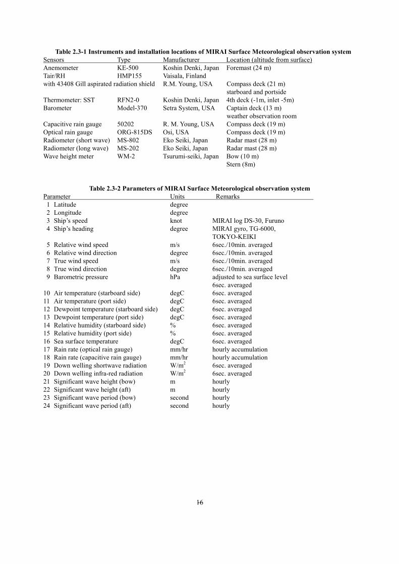
Table 2.3-1 Instruments and installation locations of MIRAI Surface Meteorological observation system Sensors Type Manufacturer Location (altitude from surface) Anemometer KE-500 Koshin Denki, Japan Foremast (24 m) Tair/RH HMP155 Vaisala, Finland with 43408 Gill aspirated radiation shield R.M. Young, USA Compass deck (21 m) starboard and portside Thermometer: SST RFN2-0 Koshin Denki, Japan 4th deck (-1m, inlet -5m) Barometer Model-370 Setra System, USA Captain deck (13 m) weather observation room Capacitive rain gauge 50202 R. M. Young, USA Compass deck (19 m) Optical rain gauge ORG-815DS Osi, USA Compass deck (19 m) Radiometer (short wave) MS-802 Eko Seiki, Japan Radar mast (28 m) Radiometer (long wave) MS-202 Eko Seiki, Japan Radar mast (28 m) Wave height meter WM-2 Tsurumi-seiki, Japan Bow (10 m) Stern (8m)
Table 2.3-2 Parameters of MIRAI Surface Meteorological observation system Parameter Units Remarks 1 Latitude degree 2 Longitude degree 3 Ship’s speed knot MIRAI log DS-30, Furuno 4 Ship’s heading degree MIRAI gyro, TG-6000, TOKYO-KEIKI 5 Relative wind speed m/s 6sec./10min. averaged 6 Relative wind direction degree 6sec./10min. averaged 7 True wind speed m/s 6sec./10min. averaged 8 True wind direction degree 6sec./10min. averaged 9 Barometric pressure hPa adjusted to sea surface level
6sec. averaged 10 Air temperature (starboard side) degC 6sec. averaged 11 Air temperature (port side) degC 6sec. averaged 12 Dewpoint temperature (starboard side) degC 6sec. averaged 13 Dewpoint temperature (port side) degC 6sec. averaged 14 Relative humidity (starboard side) % 6sec. averaged 15 Relative humidity (port side) % 6sec. averaged 16 Sea surface temperature degC 6sec. averaged 17 Rain rate (optical rain gauge) mm/hr hourly accumulation 18 Rain rate (capacitive rain gauge) mm/hr hourly accumulation 19 Down welling shortwave radiation W/m2 6sec. averaged 20 Down welling infra-red radiation W/m2 6sec. averaged 21 Significant wave height (bow) m hourly 22 Significant wave height (aft) m hourly 23 Significant wave period (bow) second hourly 24 Significant wave period (aft) second hourly

--
17
Table 2.3-3 Instruments and installation locations of SOAR system Sensors (Meteorological) Type Manufacturer Location (altitude from surface) Anemometer 05106 R.M. Young, USA Foremast (25 m) Barometer PTB210 Vaisala, Finland with 61002 Gill pressure port R.M. Young, USA Foremast (23 m) Capacitive rain gauge 50202 R.M. Young, USA Foremast (24 m) Tair/RH HMP155 Vaisala, Finland with 43408 Gill aspirated radiation shield R.M. Young, USA Foremast (23 m) Optical rain gauge ORG-815DR Osi, USA Foremast (24 m) Sensors (PRP) Type Manufacturer Location (altitude from surface) Radiometer (short wave) PSP Epply Labs, USA Foremast (25 m) Radiometer (long wave) PIR Epply Labs, USA Foremast (25 m) Fast rotating shadowband radiometer Yankee, USA Foremast (25 m) Sensor (PAR) Type Manufacturer Location (altitude from surface) PAR sensor PUV-510 Biospherical Instru ments Inc., USA Navigation deck (18m)
Table 2.3-4 Parameters of SOAR system (JamMet) Parameter Units Remarks 1 Latitude degree 2 Longitude degree 3 SOG knot 4 COG degree 5 Relative wind speed m/s 6 Relative wind direction degree 7 Barometric pressure hPa 8 Air temperature degC 9 Relative humidity %
10 Rain rate (optical rain gauge) mm/hr 11 Precipitation (capacitive rain gauge) mm reset at 50 mm 12 Down welling shortwave radiation W/m2 13 Down welling infra-red radiation W/m2 14 Defuse irradiance W/m2 15 PAR microE/cm2/sec 16 UV305nm microW/ cm2/nm 17 UV320nm microW/ cm2/nm 18 UV340nm microW/ cm2/nm 19 UV380nm microW/ cm2/nm

--
18
Fig. 2.3-1 Time series of surface meteorological parameters during this cruise (Leg1).

--
19
Fig. 2.3-1 Continued (Leg1).

--
20
Fig. 2.3-1 Continued (Leg2).

--
21
2.4 Thermo-Salinograph and Related Measurements February 22, 2016
(1) Personnel
Hiroshi Uchida (JAMSTEC)
Kosei Sasaoka (JAMSTEC)
Masahiro Orui (MWJ)
Misato Kuwahara (MWJ)
Keitaro Matsumoto (MWJ)
Haruka Tamada (MWJ)
(2) Objectives
The objective is to collect sea surface salinity, temperature, dissolved oxygen, fluorescence, turbidity, and nitrate
data continuously along the cruise track.
(3) Materials and methods The Continuous Sea Surface Water Monitoring System (Marine Works Japan Co, Ltd.) has seven sensors and
automatically measures salinity, temperature, dissolved oxygen, fluorescence, and turbidity in sea surface water every one minute. This system is located in the sea surface monitoring laboratory and bottom of the ship and connected to shipboard LAN system. Measured data along with time and location of the ship were displayed on a monitor and stored in a desktop computer. The sea surface water was continuously pumped up to the laboratory from about 5 m water depth and flowed into the system through a vinyl-chloride pipe. One thermometer is located just before the sea water pump at bottom of the ship. The flow rate of the surface seawater was controlled to be about 1.2 L/min. Periods of measurement, maintenance and problems are listed in Table 2.4.1.
A chemical-free nitrate sensor was also used with the Continuous Sea Surface Water Monitoring System. The nitrate sensor was attached using a flow cell next to the thermo-salinograph.
Software and sensors used in this system are listed below.
i. Software
Seamoni-kun Ver.1.50
ii. Sensors
Temperature and conductivity sensor
Model: SBE 45, Sea-Bird Electronics, Inc.
Serial number: 4552788-0264
Pre-cruise calibration: 30 August 2014, Sea-Bird Electronics, Inc.
Bottom of ship thermometer
Model: SBE 38, Sea-Bird Electronics, Inc.
Serial number: 3852788-0457
Pre-cruise calibration: 31 October 2014, Sea-Bird Electronics, Inc.

--
22
Dissolved oxygen sensor
Model: RINKO-II, JFE Adantech Co. Ltd.
Serial number: 0013
Pre-cruise calibration: 10 May 2015, JAMSTEC
Model: OPTODE 3835, Aanderaa Data Instruments, AS.
Serial number: 1519
Pre-cruise calibration: 13 May 2015, JAMSTEC
Fluorometer and turbidity sensor
Model: C3, Turner Designs, Inc. Serial number: 2300384
Nitrate sensor
Model: Deep SUNA, Satlantic, LP. Serial number: 0385
Table 2.4.1. Events of the Continuous Sea Surface Water Monitoring System operation. System Date
[UTC]
System Time
[UTC]
Event
2015/12/23 19:00 Logging for leg 1 start
2015/12/24 05:23–06:07 Flow rate for a line of RINKO and
Optode would be small, though both
data seem to be normal.
2015/12/29 10:11 Logging stop for C3/filter cleaning
2015/12/29 11:23 Logging restart
2016/01/05 11:27 Logging stop for C3/filter cleaning
2016/01/05 13:05 Logging restart
2016/01/05 13:05–13:25 Optode was unstable.
2016/01/11 22:00 Logging for leg 1 end
2016/01/17 13:35 Logging for leg 2 start
2016/01/23 06:23 Logging for leg 2 end
(4) Pre-cruise calibration
Pre-cruise sensor calibrations for the SBE 45 and SBE 38 were performed at Sea-Bird Electronics, Inc.
Pre-cruise sensor calibrations for the oxygen sensors were performed at JAMSTEC. The oxygen sensors were
immersed in fresh water in a 1-L semi-closed glass vessel, which was immersed in a temperature-controlled water bath.
Temperature of the water bath was set to 1, 10, 20 and 29ºC. Temperature of the fresh water in the vessel was measured

--
23
by a thermistor thermometer (expanded uncertainty of smaller than 0.01ºC, ARO-PR, JFE Advantech, Co., Ltd.). At each
temperature, the fresh water in the vessel was bubbled with standard gases (4, 10, 17 and 25% oxygen consisted of the
oxygen-nitrogen mixture, whose relative expanded uncertainty is 0.5%) for more than 30 minutes to insure saturation.
Absolute pressure of the vessel headspace was measured by a reference quartz crystal barometer (expanded uncertainty
of 0.01% of reading) and ranged from about 1040 to 1070 hPa. The data were averaged over 5 minutes at each calibration
point (a matrix of 24 points). As a reference, oxygen concentration of the fresh water in the calibration vessel was
calculated from the oxygen concentration of the gases, temperature and absolute pressure at the water depth (about 8 cm)
of the sensor’s sensing foil as follows:
O2 (µmol/L) = {1000 × c(T) × (Ap – pH2O)} / {0.20946 × 22.3916 × (1013.25 – pH2O)}
where c(T) is the oxygen solubility, Ap is absolute pressure [in hPa], and pH2O is the water vapor pressure [in hPa].
The RINKO was calibrated by the modified Stern-Volmer equation slightly modified from a method by Uchida et al.
(2010):
O2 (µmol/L) = [(V0 / V)E – 1] / Ksv
where V is raw phase difference, V0 is raw phase difference in the absence of oxygen, Ksv is Stern-Volmer constant. The
coefficient E corrects nonlinearity of the Stern-Volmer equation. The V0 and the Ksv are assumed to be functions of
temperature as follows.
Ksv = C0 + C1 × T + C2 × T2
V0 = 1 + C3 × T
V = C4 + C5 × Vb
where T is CTD temperature (°C) and Vb is raw output. The oxygen concentration is calculated using accurate
temperature data from the SBE 45 instead of temperature data from the RINKO. The calibration coefficients were as
follows:
C0 = 5.048509438066593e-03
C1 = 2.212851808960770e-04
C2 = 3.735982971782336e-06
C3 = -7.847113805097885e-04
C4 = 3.011495646664952e-02
C5 = 0.1926948014214438
E = 1.5
(5) Data processing and post-cruise calibration
Data from the Continuous Sea Surface Water Monitoring System were obtained at 1 minute intervals. Data from the
nitrate sensor were obtained at 2 minute intervals and linearly interpolated at 1 minute intervals.
These data were processed as follows. Spikes in the temperature and salinity data were removed using a median
filter with a window of 3 scans (3 minutes) when difference between the original data and the median filtered data was
larger than 0.1ºC for temperature and 0.5 for salinity. Data gaps were linearly interpolated when the gap was ≤ 13
minutes. Fluoromete and turbidity data were low-pass filtered using a median filter with a window of 3 scans (3 minutes)

--
24
to remove spikes. Raw data from the RINKO oxygen sensor, fluorometer, turbidity and nitrate data were low-pass
filtered using a Hamming filter with a window of 15 scans (15 minutes).
A slope correction was applied to the nitrate sensor before post-cruise calibration. RMNS (Reference Material for
Nutrients in Seawater, Kanso Technos Co., Ltd., Osaka, Japan) lot BU and CA were measured by the nitrate sensor
during the cruise (Fig. 2.4.1 and Table 2.4.2) and a slope (a1) for the correction was estimated to be 0.897966 on average
from the following equation:
NRA [µmol/kg] = a0 + a1 NRAorg
where NRA is corrected nitrate concentration, NRAorg is raw data, and a0 is the offset at the time of RMNS measurement.
Salinity (S [PSU]), dissolved oxygen (O [µmol/kg]), fluorescence (Fl [RFU]), and nitrate (NRA [µmol/kg]) data
were corrected using the water sampled data. Details of the measurement methods are described in Sections 3.2, 3.4, 3.5,
and 3.10 for salinity, dissolved oxygen, nitrate and chlorophyll-a, respectively. Corrected salinity (Scor), dissolved oxygen
(Ocor), estimated chlorophyll a (Chl-a), and nitrate (NRAcor) were calculated from following equations
Scor [PSU] = c0 + c1 S + c2 t
Ocor [µmol/kg] = c0 + c1 O + c2 T + c3 t
Chl-a [µg/L] = c0 + c1 Fl
NRAcor [µmol/kg] = a1 NRAorg + c0 + c1 t
where S is practical salinity, t is days from a reference time (2015/12/23 19:00 [UTC]), T is temperature in ºC. The best
fit sets of calibration coefficients (c0~c3) were determined by a least square technique to minimize the deviation from the
water sampled data. The calibration coefficients were listed in Table 2.4.2. Comparisons between the Continuous Sea
Surface Water Monitoring System data and water sampled data are shown in Figs. 2.4.2, and 2.4.3.
For fluorometer data, water sampled data obtained at night [PAR (Photosynthetically Available Radiation) < 50
µE/(m2 sec)] were used for the calibration, since sensitivity of the fluorometer to chlorophyll a is different at nighttime
and daytime (Section 2.4 in Uchida et al., 2015). Sensitivity of the fluorometer to chlorophyll a may also have regional
differences. Therefore, slope (c1) of the calibration coefficients will be changed between legs 1 and 2.
Post-cruise calibration of the nitrate sensor will be carried out after quality control of the water sampled nitrate data
is finished.
(6) References
Uchida, H., G. C. Johnson, and K. E. McTaggart (2010): CTD oxygen sensor calibration procedures, The GO-SHIP
Repeat Hydrography Manual: A collection of expert reports and guidelines, IOCCP Rep., No. 14, ICPO Pub. Ser. No.
134.
Uchida, H., K. Katsumata, and T. Doi (2015): WHP P14S, S04I Revisit Data Book, JASTEC, Yokosuka, 187 pp.
Table 2.4.2. Nitrate concentration measured by the nitrate sensor for RMNS lot BU (3.888±0.063 [k=2] µmol/kg) and lot
CA (19.66±0.15 [k = 2] µmol/kg). Offset (a0) of the correction equation (see text for detail) at the time of
measurement was also shown.

--
25
-------------------------------------------------------------------------------------------------------------------------------
Date RMNS lot BU RMNS lot CA a0
-------------------------------------------------------------------------------------------------------------------------------
2016/01/05 11:40-11:47 –17.71±0.58 –0.20±0.88 19.815
2016/01/05 12:02-12:09 8.70±0.16 26.46±0.17 –4.012
2016/01/10 00:06-00:11 –11.08±0.38 6.11±0.29 14.005
2016/01/17 05:51-05:58 9.65±0.18 27.84±0.20 –5.058
2016/01/23 06:54-07:01 –17.82±0.64 –0.61±0.45 20.049
-------------------------------------------------------------------------------------------------------------------------------

--
26
Table 2.4.3. Calibration coefficients for the salinity, dissolved oxygen, chlorophyll a, and nitrate.
-------------------------------------------------------------------------------------------------------------------------------
c0 c1 c2 c3
-------------------------------------------------------------------------------------------------------------------------------
Salinity
9.031385e-02 0.9976929 1.379279e-04
Dissolved oxygen
9.417670 0.9360383 0.0 -8.925093e-03
Chlorophyll a
Nitrate
-------------------------------------------------------------------------------------------------------------------------------
Figure 2.4.1. Results of RMNS measurements by the nitrate sensor. Differences between measured value and certified

--
27
value are shown. Error bar shows the standard deviation of the measurements.
Figure 2.4.2. Comparison between TSG salinity (red: before correction, green: after correction) and sampled salinity.

--
28
Figure 2.4.3. Comparison between TSG oxygen (red: before correction, green: after correction) and sampled oxygen.

--
29
2.5. Surface pCO2 (1) Personnel
Akihiko Murata (JAMSTEC)
Atsushi Ono (NIO)
Makoto Takada (MWJ)
Tomonori Watai (MWJ)
(2) Objective
Concentrations of CO2 in the atmosphere are now increasing at a rate of about 2.0 ppmv y–1 owing to human
activities such as burning of fossil fuels, deforestation, and cement production. It is an urgent task to estimate as
accurately as possible the absorption capacity of the oceans against the increased atmospheric CO2, and to clarify the
mechanism of the CO2 absorption, because the magnitude of the anticipated global warming depends on the levels of
CO2 in the atmosphere, and because the ocean currently absorbs 1/3 of the 6 Gt of carbon emitted into the atmosphere
each year by human activities.
In this cruise, we were aimed at quantifying how much anthropogenic CO2 absorbed in the surface ocean in the
eastern part of the Indian Ocean and in the western North Pacific. For the purpose, we measured pCO2 (partial pressure
of CO2) in the atmosphere and surface seawater along the observation line.
(3) Apparatus
Concentrations of CO2 in the atmosphere and the sea surface were measured continuously during the cruise
using an automated system with a non-dispersive infrared (NDIR) analyzer (Li-COR LI-7000). The automated system
(Nippon ANS) was operated by about one and a half hour cycle. In one cycle, standard gasses, marine air and an air in a
headspace of an equilibrator were analyzed subsequently. The nominal concentrations of the standard gas were 270, 330,
359 and 419 ppmv. The standard gases will be calibrated after the cruise.
The marine air taken from the bow was introduced into the NDIR by passing through a mass flow controller,
which controlled the air flow rate at about 0.6 – 0.8 L/min, a cooling unit, a perma-pure dryer (GL Sciences Inc.) and a
desiccant holder containing Mg(ClO4)2.
A fixed volume of the marine air taken from the bow was equilibrated with a stream of seawater that flowed at
a rate of 4.0 – 5.0 L/min in the equilibrator. The air in the equilibrator was circulated with a pump at 0.7-0.8L/min in a
closed loop passing through two cooling units, a perma-pure dryer (GL Science Inc.) and a desiccant holder containing
Mg(ClO4)2.
(4) Results
Concentrations of CO2 (xCO2) of marine air and surface seawater are shown in Fig. 2.5.1, together with SST.

--
30
Fig. 2.5.1. Preliminary results of concentrations of CO2 (xCO2) in atmosphere (upper panel) and surface seawater
(lower panel) observed during MR15-05.

--
31
2.6 Ceilometer observation (1) Personnel
Katsuro Katsumata JAMSTEC: Principal investigator - leg1 - Akihiko Murata JAMSTEC: Principal investigator - leg2 - Wataru Tokunaga Global Ocean Development Inc., (GODI) - leg1 - Tetsuya Kai GODI - leg1 - Koichi Inagaki GODI - leg2 - Yutaro Murakami GODI - leg1, leg2 - Ryo Kimura MIRAI crew - leg1 - Masanori Murakami MIRAI crew - leg2 -
(2) Objectives
The information of cloud base height and the liquid water amount around cloud base is important to understand the process on formation of the cloud. As one of the methods to measure them, the ceilometer observation was carried out.
(3) Parameters
1. Cloud base height [m]. 2. Backscatter profile, sensitivity and range normalized at 10 m resolution. 3. Estimated cloud amount [oktas] and height [m]; Sky Condition Algorithm.
(4) Methods
We measured cloud base height and backscatter profile using ceilometer (CL51, VAISALA, Finland). Major parameters for the measurement configuration are shown in Table 2.6-1;
Table 2.6-1 Major parameters
---------------------------------------------------------------------------------------------------------------------- Laser source: Indium Gallium Arsenide (InGaAs) Diode Transmitting center wavelength: 910±10 nm at 25 degC Transmitting average power: 19.5 mW Repetition rate: 6.5 kHz Detector: Silicon avalanche photodiode (APD) Responsibility at 905 nm: 65 A/W Cloud detection range: 0 ~ 13 km Measurement range: 0 ~ 15 km Resolution: 10 meter in full range Sampling rate: 36 sec Sky Condition: Cloudiness in octas (0 ~ 9) (0: Sky Clear, 1: Few, 3: Scattered, 5-7: Broken, 8: Overcast, and 9: Vertical
Visibility) -----------------------------------------------------------------------------------------------------------------------
On the archive dataset, cloud base height and backscatter profile are recorded with the resolution of 10 m (33 ft).
(5) Preliminary results
Fig.2.6-1 shows the time series of 1st, 2nd and 3rd lowest cloud base height during the cruise. (6) Data archives
The raw data obtained during this cruise will be submitted to the Data Management Group (DMG) of JAMSTEC.

--
32
(7) Remarks (Times in UTC)
i) The following periods, the observation were carried out. Leg1: 18:51, 23 Dec. 2015 to 22:40, 10 Jan. 2016 Leg2: 13:35, 17 Jan. 2016 to 23:50, 24 Jan. 2016
ii) The following time, the window was cleaned.
01:27, 27 Dec. 2015 01:10, 03 Jan. 2016 01:30, 21 Jan. 2016

--
33
Fig. 2.6-1 1st, 2nd and 3rd lowest cloud base height during this cruise (Leg1).
Fig. 2.6-1 Continued (Leg2).

--
34
2.7 Surface CO2 fluxes Kei Shiomi (JAXA) Shuji KAWAKAMI (JAXA) Masakatsu NAKAJIMA (JAXA) Yoshiyuki NAKANO (JAMSTEC) (1) Objective Greenhouse gases Observing SATellite (GOSAT) was launched on 23 January 2009 in order to observe the global distributions of atmospheric greenhouse gas concentrations: column-averaged dry-air mole fractions of carbon dioxide (CO2) and methane (CH4). A network of ground-based high-resolution Fourier transform spectrometers provides essential validation data for GOSAT. Vertical CO2 profiles obtained during ascents and descents of commercial airliners equipped with the in-situ CO2 measuring instrument are also used for the GOSAT validation. Because such validation data are obtained mainly over land, there are very few data available for the validation of the over-sea GOSAT products. The objectives of our research are to acquire the validation data over the Indian Ocean and the tropical Pacific Ocean using an automated compact instrument, to compare the acquired data with the over-sea GOSAT products, and to develop a simple estimation of the carbon flux between the ocean and the atmosphere from GOSAT data. (2) Description of instruments deployed The column-averaged dry-air mole fractions of CO2 and CH4 can be estimated from absorption by atmospheric CO2 and CH4 that is observed in a solar spectrum. An optical spectrum analyzer (OSA, Yokogawa M&I co., AQ6370) was used for measuring the solar absorption spectra in the near-infrared spectral region. A solar tracker (PREDE co., ltd.) and a small telescope (Figure 1) collected the sunlight into the optical fiber that was connected to the OSA. The solar tracker searches the sun every one minute until the sunlight with a defined intensity. The measurements of the solar spectra were performed during solar zenith angles less than 80°. (3) Analysis method
The CO2 absorption spectrum at the 1.6 µm band measured with the OSA is shown in Figure 2. The absorption spectrum can be simulated based on radiative transfer theory using assumed atmospheric profiles of pressure, temperature, and trace gas concentrations. The column abundance of CO2 (CH4) was retrieved by adjusting the assumed CO2 (CH4) profile to minimize the differences between the measured and simulated spectra.
Figure 1. Solar tracker and telescope. The sunlight
collected into optical fiber was introduced into the
OSA that was installed in an observation room in
the MIRAI.

--
35
Figure 3 shows an example of spectral fit performed for the spectral region with the CO2 absorption lines. The column-averaged dry-air mole fraction of CO2 (CH4) was obtained by taking the ratio of the CO2 (CH4) column to the dry-air column.
Figure 2. 1.6 µm CO2 absorption spectrum measured with the OSA.
Figure 3. Spectral fit performed for the 6297–6382 cm−1 region using an OSA spectrum. Open
diamonds denote the measured spectrum, and the solid line denotes the spectrum calculated
from the retrieval result. The residual between the measured and calculated spectra is also
shown.

--
36
(4) Preliminary results The observations were made from December 24, 2015 to January 24, 2016 continuously in daytime (Table 1
and Figure 2).
DateStart
Time(JST)End
Time(JST)2015/12/24 09:14 19:342015/12/25 08:14 19:362015/12/26 08:14 19:442015/12/27 08:09 18:432015/12/28 07:44 19:312015/12/29 07:39 19:372015/12/30 07:55 19:492015/12/31 07:47 19:292016/01/01 07:50 19:452016/01/02 07:53 19:382016/01/03 07:56 18:112016/01/04 07:58 16:372016/01/05 08:00 19:032016/01/06 08:05 18:542016/01/07 08:04 19:152016/01/08 08:06 19:062016/01/09 08:08 19:102016/01/18 07:32 17:152016/01/19 07:38 13:162016/01/20 07:38 16:382016/01/21 07:38 16:382016/01/24 09:15 16:10
CO2 observations
Table 1. Period of CO2 observations Figure 2. Locations of CO2 observations
(5) Data archive The column-averaged dry-air mole fractions of CO2 and CH4 retrieved from the OSA spectra will be
submitted to JAMSTEC Data Management Group (DMG).

2.8. Radars and Disdrometers
(1) Personnel
Masaki Katsumata (JAMSTEC)
Yuki Kaneko (JAXA)
Kazuhide Yamamoto (JAXA) (not on board)
(2) Objectives
Accurate measurement of the precipitating particle on its amount, phase and their spatiotemporal distributions is crucial to understand the climate system, thru evaluating the latent heating of the atmosphere, radiative heating of the atmosphere and ocean, fresh water flux into the ocean, etc. To better measure and understand the global precipitation, we deployed various instruments to measure the various characteristics of the precipitation on R/V Mirai which deployed globally. The objective of this observation is (a) to reveal various characteristics of the rainfall, depends on the type, temporal stage, etc. of the precipitating clouds, (b) to retrieve the coefficient to convert radar reflectivity to the rainfall amount, and (c) to validate the algorithms and the product of the satellite-borne precipitation radars; TRMM/PR and GPM/DPR.
(3) Apparatus
(3-1) Disdrometers
Four different types of disdrometers are utilized to obtain better reasonable and accurate value on the moving vessel. Three of the disdrometers and one optical rain gauge are installed in one place, the starboard side on the roof of the anti-rolling system of R/V Mirai, as in Fig. 2.8-1. One of the disdrometers named “micro rain radar” is installed at the starboard side of the anti-rolling systems (see Fig. 2.8-2).
The details of the sensors are described below. All the sensors archive data every one minute.
Fig. 2.8-1: The three disdrometers (Parsivel, LPM and Joss-Waldvogel disdrometer) and an optical rain gauge, installed on the roof of the anti-rolling tank.
(3-1-1) Joss-Waldvogel type disdrometer The “Joss-Waldvogel-type” disdrometer system (RD-80, Disdromet Inc.) (hereafter JW) equipped a
microphone on the top of the sensor unit. When a raindrop hit the microphone, the magnitude of induced sound is

--
38
converted to the size of raindrops. The logging program “DISDRODATA” determines the size as one of the 20 categories as in Table 2.8-1, and accumulates the number of raindrops at each category. The rainfall amount could be also retrieved from the obtained drop size distribution. The number of raindrops in each category, and converted rainfall amount, are recorded every one minute.
(3-1-2) Laser Precipitation Monitor (LPM) optical disdrometer
The “Laser Precipitation Monitor (LPM)” (Adolf Thies GmbH & Co) is an optical disdrometer. The instrument consists of the transmitter unit which emit the infrared laser, and the receiver unit which detects the intensity of the laser come thru the certain path length in the air. When a precipitating particle fall thru the laser, the received intensity of the laser is reduced. The receiver unit detect the magnitude and the duration of the reduction and then convert them onto particle size and fall speed. The sampling volume, i.e. the size of the laser beam “sheet”, is 20 mm (W) x 228 mm (D) x 0.75 mm (H).
The number of particles are categorized by the detected size and fall speed and counted every minutes. The categories are shown in Table 2.8-2.
(3-1-3) “Parsivel” optical disdrometer
The “Parsivel” (OTT Hydromet GmbH) is another optical disdrometer. The principle is same as the LPM. The sampling volume, i.e. the size of the laser beam “sheet”, is 30 mm (W) x 180 mm (D). The categories are shown in Table 2.8-3.
(3-1-4) Optical rain gauge
The optical rain gauge, which detect scintillation of the laser by falling raindrops, is installed beside the above three disdrometers to measure the exact rainfall. The ORG-815DR (Optical Scientific Inc.) is utilized with the controlling and recording software (manufactured by Sankosha Co.).

--
39
Table 2.8-1: Category number and corresponding size of the raindrop for JW disdrometer. Category Corresponding size range [mm]
1 0.313 - 0.405 2 0.405 - 0.505 3 0.505 - 0.696 4 0.696 - 0.715 5 0.715 - 0.827 6 0.827 - 0.999 7 0.999 - 1.232 8 1.232 - 1.429 9 1.429 - 1.582
10 1.582 - 1.748 11 1.748 - 2.077 12 2.077 - 2.441 13 2.441 - 2.727 14 2.727 - 3.011 15 3.011 - 3.385 16 3.385 - 3.704 17 3.704 - 4.127 18 4.127 - 4.573 19 4.573 - 5.145 20 5.145 or larger

--
40
Table 2.8-2: Categories of the size and the fall speed for LPM. Particle Size Fall Speed
Class Diameter [mm]
Class width [mm]
Class Speed [m/s]
Class width [m/s]
1 ≥ 0.125 0.125 1 ≥ 0.000 0.200 2 ≥ 0.250 0.125 2 ≥ 0.200 0.200 3 ≥ 0.375 0.125 3 ≥ 0.400 0.200 4 ≥ 0.500 0.250 4 ≥ 0.600 0.200 5 ≥ 0.750 0.250 5 ≥ 0.800 0.200 6 ≥ 1.000 0.250 6 ≥ 1.000 0.400 7 ≥ 1.250 0.250 7 ≥ 1.400 0.400 8 ≥ 1.500 0.250 8 ≥ 1.800 0.400 9 ≥ 1.750 0.250 9 ≥ 2.200 0.400
10 ≥ 2.000 0.500 10 ≥ 2.600 0.400 11 ≥ 2.500 0.500 11 ≥ 3.000 0.800 12 ≥ 3.000 0.500 12 ≥ 3.400 0.800 13 ≥ 3.500 0.500 13 ≥ 4.200 0.800 14 ≥ 4.000 0.500 14 ≥ 5.000 0.800 15 ≥ 4.500 0.500 15 ≥ 5.800 0.800 16 ≥ 5.000 0.500 16 ≥ 6.600 0.800 17 ≥ 5.500 0.500 17 ≥ 7.400 0.800 18 ≥ 6.000 0.500 18 ≥ 8.200 0.800 19 ≥ 6.500 0.500 19 ≥ 9.000 1.000 20 ≥ 7.000 0.500 20 ≥ 10.000 10.000 21 ≥ 7.500 0.500 22 ≥ 8.000 unlimited

--
41
Table 2.8-3: Categories of the size and the fall speed for Parsivel. Particle Size Fall Speed
Class Average Diameter [mm]
Class spread [mm]
Class Average Speed [m/s]
Class Spread [m/s]
1 0.062 0.125 1 0.050 0.100 2 0.187 0.125 2 0.150 0.100 3 0.312 0.125 3 0.250 0.100 4 0.437 0.125 4 0.350 0.100 5 0.562 0.125 5 0.450 0.100 6 0.687 0.125 6 0.550 0.100 7 0.812 0.125 7 0.650 0.100 8 0.937 0.125 8 0.750 0.100 9 1.062 0.125 9 0.850 0.100
10 1.187 0.125 10 0.950 0.100 11 1.375 0.250 11 1.100 0.200 12 1.625 0.250 12 1.300 0.200 13 1.875 0.250 13 1.500 0.200 14 2.125 0.250 14 1.700 0.200 15 2.375 0.250 15 1.900 0.200 16 2.750 0.500 16 2.200 0.400 17 3.250 0.500 17 2.600 0.400 18 3.750 0.500 18 3.000 0.400 19 4.250 0.500 19 3.400 0.400 20 4.750 0.500 20 3.800 0.400 21 5.500 1.000 21 4.400 0.800 22 6.500 1.000 22 5.200 0.800 23 7.500 1.000 23 6.000 0.800 24 8.500 1.000 24 6.800 0.800 25 9.500 1.000 25 7.600 0.800 26 11.000 2.000 26 8.800 1.600 27 13.000 2.000 27 10.400 1.600 28 15.000 2.000 28 12.000 1.600 29 17.000 2.000 29 13.600 1.600 30 19.000 2.000 30 15.200 1.600 31 21.500 3.000 31 17.600 3.200 32 24.500 3.000 32 20.800 3.200

--
42
(3-2) Micro rain radar
The MRR-2 (METEK GmbH) was utilized. The specifications are in Table 2.8-4. The antenna unit was installed at the starboard side of the anti-rolling systems (see Fig. 2.8-2), and wired to the junction box and laptop PC inside the vessel.
The data was averaged and stored every one minute. The vertical profile of each parameter was obtained every 200 meters in range distance (i.e. height) up to 6200 meters, i.e. well beyond the melting layer. The drop size distribution is recorded, as well as radar reflectivity, path-integrated attenuation, rain rate, liquid water content and fall velocity.
Fig. 2.8-2: The micro rain radar, installed on the starboard side of the anti-rolling tank.
Table 2.8-4: Specifications of the MRR-2. Transmitter power 50 mW Operating mode FM-CW Frequency 24.230 GHz
(modulation 1.5 to 15 MHz) 3dB beam width 1.5 degrees Spurious emission < -80 dBm / MHz Antenna Diameter 600 mm Gain 40.1 dBi
(3-3) Ka-band radar
The Ka-band radar (Manufactured by Mitsubishi Electric Co.) was utilized. The specifications are in Table 2.8-5.
The antenna unit was installed at the stern (starboard side) of the vessel (see Fig. 2.8-x), and wired to the signal
processing unit inside the vessel (so-called “dry labo”). Antenna direction is fixed to zenith relative to the ship.
Table 2.8-5: Specifications of the Ka-band radar
Frequency 35.25 GHz (Ka-band)

--
43
Modulation Principle FMCW Minimum Detect Zm -20 dBZ at 10 km Minimum Range Resolution 12.5 m Minimum Time Resolution 10 sec Niquist Velocity ±10.6 m/s Observable range From 500 m to 30 km
(Depends on the observation mode) Antenna beam width 0.6 deg Antenna sidelobe < 25 dBZ Radar Variables Radar reflectivity and Doppler spectrum
Fig. 2.8-3: The Ka-band radar system. (left) Antenna part, at the right-side of the stern of the upper deck. (right) Signal processer part, in the “dry labo.”
(3-3) C-band radar
The C-band polarimetric weather radar in R/V Mirai was utilized. The basic specifications are in Table 2.4-4. The antenna is controlled to point the commanded ground-relative direction, by controlling the azimuth and elevation to cancel the ship attitude (roll, pitch and yaw) detected by the laser gyro. The Doppler velocity is also corrected by subtracting the ship movement in beam direction.
For the maintenance, internal signals of the radar are checked and calibrated at the beginning and the end of the cruise. Meanwhile, the following parameters are checked daily; (1) frequency, (2) mean output power, (3) pulse width, and (4) PRF (pulse repetition frequency).
During the cruise, parameters in Table 2.x-x were obtained. Scan strategies are shown in Table 2.x-x. The radar is operated to repeat the cycle every 6 minutes basically, while every 30 minutes to obtain surveillance PPI. A dual PRF mode is used for a volume scan. For vertical pointing scan and surveillance PPI scans, a single PRF mode is used.
Table 5.3-1 Scan settings of the C-band radar in the cruise. Surveillance
PPI Scan Volume Scan
Vertical Point Scan

--
44
Repeated Cycle (min.) 30 6 6 Times in One Cycle 1 1 3 Pulse Width (long / short, in microsec)
200 / 2 64 / 1 32 / 1 32 / 1
32 / 1
Scan Speed (deg/sec)
36 18 24 36 36
PRF(s) (Hz) 400
dual PRF (ray alternative) 2000
667 833 938 1250 1333 2000 Pulses / Ray 8 26 33 27 34 37 55 64 Ray Spacing (deg.) 0.7 0.7 0.7 1.0 1.0 Azimuth (deg) Full Circle Bin Spacing (m) 150 Max. Range (km) 300 150 100 60 60 Elevation Angle(s) (deg.)
0.5 0.5 1.0, 1.8, 2.6, 3.4, 4.2, 5.1, 6.2, 7.6, 9.7, 12.2,
15.2
18.7, 23.0, 27.9, 33.5,
40.0
90
(4) Results
The data were obtained continuously thru the cruise from Dec.23, 2015 to Jan.23, 2016, except the period when Mirai was in the area where the observation is not permitted. The further analyses will be done after the cruise.
(5) Data Archive
All data obtained during this cruise will be submitted to the JAMSTEC Data Management Group (DMG).

--
45
2.9. Aerosol optical characteristics measured by Ship-borne Sky radiometer (1) Personnel
Kazuma Aoki (University of Toyama) - Principal Investigator (not on board) Tadahiro Hayasaka (Tohoku University) - Co-Investigator (not onboard) (Sky radiometer operation was supported by Global Ocean Development Inc.) (2) Objectives
Objective of this observation is to study distribution and optical characteristics of marine aerosols by using a ship-borne sky radiometer (POM-01 MKII: PREDE Co. Ltd., Japan). Furthermore, collections of the data for calibration and validation to the remote sensing data were performed simultaneously.
(3) Methods and Instruments
The sky radiometer measures the direct solar irradiance and the solar aureole radiance distribution with seven interference filters (0.34, 0.4, 0.5, 0.675, 0.87, 0.94, and 1.02 µm). Analysis of these data was performed by SKYRAD.pack version 4.2 developed by Nakajima et al. 1996.
@ Measured parameters
- Aerosol optical thickness at five wavelengths (400, 500, 675, 870 and 1020 nm) - Ångström exponent - Single scattering albedo at five wavelengths - Size distribution of volume (0.01 µm – 20 µm)
# GPS provides the position with longitude and latitude and heading direction of the vessel, and azimuth and elevation angle of the sun. Horizon sensor provides rolling and pitching angles.
(4) Preliminary results
Only data collection were performed onboard. At the time of writing, the data obtained in this cruise are under post-cruise processing at University of Toyama.
(5) Data archives
Aerosol optical data are to be archived at University of Toyama (K.Aoki, SKYNET/SKY: http://skyrad.sci.u-toyama.ac.jp/) after the quality check and will be submitted to JAMSTEC.
--
46
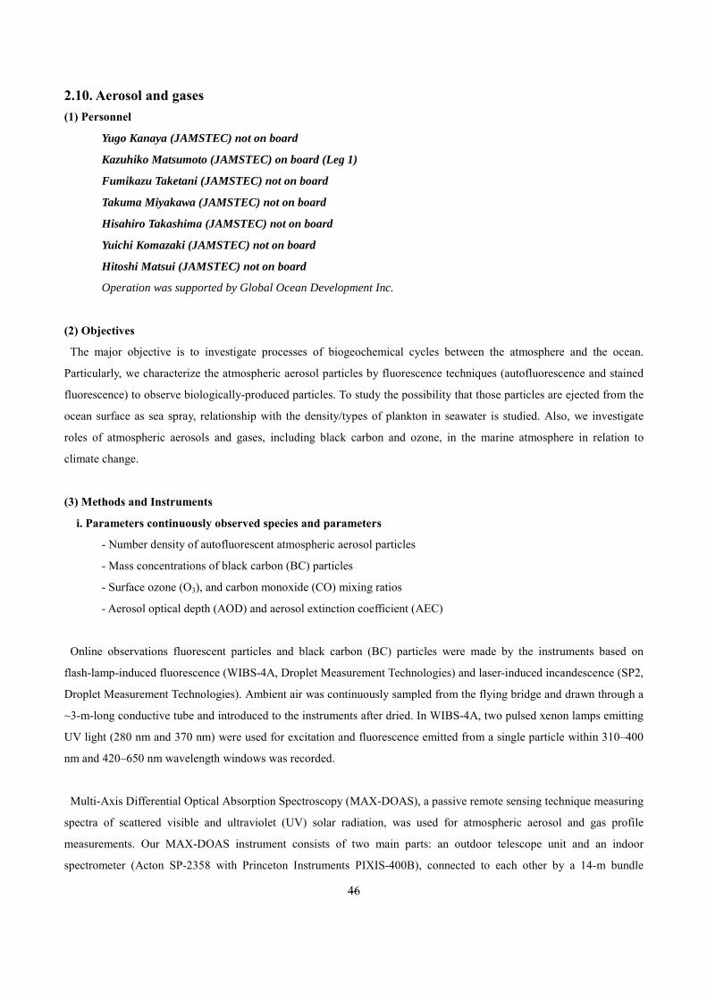
2.10. Aerosol and gases (1) Personnel
Yugo Kanaya (JAMSTEC) not on board
Kazuhiko Matsumoto (JAMSTEC) on board (Leg 1)
Fumikazu Taketani (JAMSTEC) not on board
Takuma Miyakawa (JAMSTEC) not on board
Hisahiro Takashima (JAMSTEC) not on board
Yuichi Komazaki (JAMSTEC) not on board
Hitoshi Matsui (JAMSTEC) not on board
Operation was supported by Global Ocean Development Inc.
(2) Objectives
The major objective is to investigate processes of biogeochemical cycles between the atmosphere and the ocean.
Particularly, we characterize the atmospheric aerosol particles by fluorescence techniques (autofluorescence and stained
fluorescence) to observe biologically-produced particles. To study the possibility that those particles are ejected from the
ocean surface as sea spray, relationship with the density/types of plankton in seawater is studied. Also, we investigate
roles of atmospheric aerosols and gases, including black carbon and ozone, in the marine atmosphere in relation to
climate change.
(3) Methods and Instruments
i. Parameters continuously observed species and parameters
- Number density of autofluorescent atmospheric aerosol particles
- Mass concentrations of black carbon (BC) particles
- Surface ozone (O3), and carbon monoxide (CO) mixing ratios
- Aerosol optical depth (AOD) and aerosol extinction coefficient (AEC)
Online observations fluorescent particles and black carbon (BC) particles were made by the instruments based on
flash-lamp-induced fluorescence (WIBS-4A, Droplet Measurement Technologies) and laser-induced incandescence (SP2,
Droplet Measurement Technologies). Ambient air was continuously sampled from the flying bridge and drawn through a
~3-m-long conductive tube and introduced to the instruments after dried. In WIBS-4A, two pulsed xenon lamps emitting
UV light (280 nm and 370 nm) were used for excitation and fluorescence emitted from a single particle within 310‒400
nm and 420‒650 nm wavelength windows was recorded.
Multi-Axis Differential Optical Absorption Spectroscopy (MAX-DOAS), a passive remote sensing technique measuring
spectra of scattered visible and ultraviolet (UV) solar radiation, was used for atmospheric aerosol and gas profile
measurements. Our MAX-DOAS instrument consists of two main parts: an outdoor telescope unit and an indoor
spectrometer (Acton SP-2358 with Princeton Instruments PIXIS-400B), connected to each other by a 14-m bundle

--
47
optical fiber cable. The line of sight was in the directions of the portside of the vessel and the multiple elevation angles,
1.5, 3, 5, 10, 20, 30, 90 degrees, were scanned repeatedly (every ~15-min) using a movable prism. For the selected
spectra recorded with elevation angles with good accuracy, DOAS spectral fitting was performed to quantify the slant
column density (SCD) of NO2 (and other gases) and O4 (O2-O2, collision complex of oxygen) for each elevation angle.
Then, the O4 SCDs were converted to the aerosol optical depth (AOD) and the vertical profile of aerosol extinction
coefficient (AEC) using an optimal estimation inversion method with a radiative transfer model. Using derived aerosol
information, retrievals of the tropospheric vertical column/profile of NO2 and other gases were made.
For ozone and CO measurements, ambient air was continuously sampled on the compass deck and drawn through
~20-m-long Teflon tubes connected to a gas filter correlation CO analyzer (Model 48C, Thermo Fisher Scientific) and a
UV photometric ozone analyzer (Model 49C, Thermo Fisher Scientific), located in the Research Information Center. The
data will be used for characterizing air mass origins.
ii. Sampling and offline analysis
During Leg 1, atmospheric aerosol particles and surface seawater samples were manually collected for the offline
measurements of stained fluorescence from particles. The collected timing and locations are listed in Table 2.10.1. The
stained fluorescence observations were made with Bioplorer KB-VKH01 (Koyo Sangyo Co.,Ltd ). Double staining with
DAPI and PI was utilized, for the detection of total and dead biological particles upon fluorescence signal from
individual particles induced by the UV and green light excitation. The atmospheric aerosol particles were directly
collected onto membrane filters to be used in the Bioplorer. The seawater samples were filtrated by the membrane filter
and then the filter was set in the Bioplorer for the stained fluorescence measurements. For reference, autofluorescence
was also analyzed by the Bioplorer before staining.
During Leg 1 and 2, ambient aerosol particles were collected along cruise track using a high-volume air sampler
(HV-525PM, SIBATA) located on the flying bridge operated at a flow rate of 500 L min-1. To avoid collecting particles
emitted from the funnel of the own vessel, the sampling period was controlled automatically by using a “wind-direction
selection system”. Coarse and fine particles separated at the diameter of 2.5 μm were collected. The filter samples
obtained during the cruise are subject to chemical analysis of aerosol composition, including water-soluble ions and trace
metals.
(4) Preliminary results
N/A (Data analysis is to be conducted.)
(5) Data archives
These data obtained in this cruise will be submitted to the Data Management Group of JAMSTEC, and will
be opened to the public via “Data Research System for Whole Cruise Information in JAMSTEC (DARWIN)” in
JAMSTEC web site.
http://www.godac.jamstec.go.jp/darwin/e

--
48
Table 2.10.1. Timing and locations of atmospheric aerosol and seawater samples for stained fluorescence analysis
No. Sample ID Type Collection timing (UTC) Latitude
(deg-min)
Longitude
(deg-min)
Depth (m)
1 MR15-05_001a aerosol Dec 26, 2015 6:50 UTC 17-11.7 S 109-22.09 E
2 MR15-05_002a aerosol Dec 29, 2015 7:10 UTC 24-22.56 S 110-35.73 E
3 MR15-05_003s seawater Dec 29, 2015 4:30 UTC 24-22.59 S 110-35.41 E 0
4 MR15-05_004a aerosol Dec 30, 2015 9:20 UTC 22-51.57 S 110-43.98 E
5 MR15-05_005s seawater Dec 29, 2015 23:31 UTC 23-23.8 S 110-40.52 E 0
6 MR15-05_006a aerosol Dec 31, 2015 7:20 UTC 20-57.96 S 110-53.24 E
7 MR15-05_007a aerosol Jan 3, 2016 8:05 UTC 15-36.15 S 111-20.07 E
8 MR15-05_008a aerosol Jan 5, 2016 5:15 UTC 13-10.18 S 111-32.49 E
9 MR15-05_009a aerosol Jan 7, 2016 4:40 UTC 10-42.94 S 111-45.81 E
10 MR15-05_010a aerosol Jan 7, 2016 23:40 UTC 10-2.79 S 111-49.87 E
11 MR15-05_011s seawater Jan 8, 2016 5:03 UTC 9-28.97 S 111-52.94 E 0
12 MR15-05_012a aerosol Jan 9, 2016 2:00 UTC 8-38.38 S 111-57.36 E
13 MR15-05_013a aerosol Jan 10, 2016 7:15 UTC 9-11.8 S 113-44.21 E

--
49
2.11 Sea Surface Gravity (1) Personnel
Katsuro Katsumata JAMSTEC: Principal investigator - leg1 - Akihiko Murata JAMSTEC: Principal investigator - leg2 - Wataru Tokunaga Global Ocean Development Inc., (GODI) - leg1 - Tetsuya Kai GODI - leg1 - Koichi Inagaki GODI - leg2 - Yutaro Murakami GODI - leg1, leg2 - Ryo Kimura MIRAI crew - leg1 - Masanori Murakami MIRAI crew - leg2 -
(2) Introduction
The local gravity is an important parameter in geophysics and geodesy. We collected gravity data at the sea surface.
(3) Parameters
Relative Gravity [CU: Counter Unit] [mGal] = (coef1: 0.9946) * [CU]
(4) Data Acquisition
We measured relative gravity using LaCoste and Romberg air-sea gravity meter S-116 (Micro-G LaCoste, LLC) during this cruise.
To convert the relative gravity to absolute gravity, we measured gravity, using portable gravity meter (CG-5, Scintrex), at Sekinehama and Yokohama as the reference points.
(5) Preliminary Results
Absolute gravity table is shown in Table 2.11-1.
Table 2.11-1. Absolute gravity table of the MR15-05 cruise
---------------------------------------------------------------------------------------------------------------------- Absolute Sea Ship Gravity at S-116 No. Date UTC Port Gravity Level Draft Sensor * Gravity mm/dd [mGal] [cm] [cm] [mGal] [mGal] ---------------------------------------------------------------------------------------------------------------------- #1 11/05 01:07 Sekinehama 980,371.87 251 607 980,372.81 12662.42 #2 01/25 06:38 Yokohama 979,741.75 196 625 979,742.56 12035.96 ---------------------------------------------------------------------------------------------------------------------- *: Gravity at Sensor = Absolute Gravity + Sea Level*0.3086/100 + (Draft-530)/100*0.2222
(6) Data Archive
Surface gravity data obtained during this cruise will be submitted to the Data Management Group (DMG) in JAMSTEC, and will be archived there.
(7) Remarks (Times in UTC)
i) The following periods, the observation was carried out. Leg1: 18:51, 23 Dec. 2015 to 22:40, 10 Jan. 2016 Leg2: 13:47, 17 Jan 2016 to 00:00, 25 Jan. 2016
ii) The following periods, depth data were available
--
50
Leg1: 19:35, 23 Dec. 2015 to 22:05, 10 Jan. 2016 Leg2: 13:47, 17 Jan 2016 to 06:26, 23 Jan. 2016

--
51
2.12 Sea Surface Magnetic Field (1) Personnel
Katsuro Katsumata JAMSTEC: Principal investigator - leg1 - Akihiko Murata JAMSTEC: Principal investigator - leg2 - Wataru Tokunaga Global Ocean Development Inc., (GODI) - leg1 - Tetsuya Kai GODI - leg1 - Koichi Inagaki GODI - leg2 - Yutaro Murakami GODI - leg1, leg2 - Ryo Kimura MIRAI crew - leg1 - Masanori Murakami MIRAI crew - leg2 -
(2) Introduction
Measurement of magnetic force on the sea is required for the geophysical investigations of marine magnetic anomaly caused by magnetization in upper crustal structure. We measured geomagnetic field using a three-component magnetometer during this cruise.
(3) Principle of ship-board geomagnetic vector measurement
The relation between a magnetic-field vector observed on-board, Hob, (in the ship's fixed coordinate system) and the geomagnetic field vector, F, (in the Earth's fixed coordinate system) is expressed as:
Hob = F + Hp (a) where , and are the matrices of rotation due to roll, pitch and heading of a ship, respectively. is a
3 x 3 matrix which represents magnetic susceptibility of the ship, and Hp is a magnetic field vector produced by a permanent magnetic moment of the ship's body. Rearrangement of Eq. (a) makes
Hob + Hbp = F (b) where = -1, and Hbp = - Hp. The magnetic field, F, can be obtained by measuring , , and
Hob, if and Hbp are known. Twelve constants in and Hbp can be determined by measuring variation of Hob with , and at a place where the geomagnetic field, F, is known.
(4) Instruments on R/V MIRAI
A shipboard three-component magnetometer system (Tierra Tecnica SFG1214) is equipped on-board R/V MIRAI. Three-axes flux-gate sensors with ring-cored coils are fixed on the fore mast. Outputs from the sensors are digitized by a 20-bit A/D converter (1 nT/LSB), and sampled at 8 times per second. Ship's heading, pitch, and roll are measured by the Inertial Navigation System (INS) for controlling attitude of a Doppler radar. Ship's position and speed data are taken from LAN every second.
(5) Data Archive
Sea surface magnetic data obtained during this cruise will be submitted to the Data Management Group (DMG) in JAMSTEC, and will be archived there.
(6) Remarks (Times in UTC)
i) The following periods, the observation were carried out. Leg1: 18:51, 23 Dec. 2015 to 22:40, 10 Jan. 2016 Leg2: 13:47, 17 Jan 2016 to 23:50, 24 Jan. 2016
ii) The following periods, we made a “figure-eight” turn (a pair of clockwise and anti-clockwise rotation) for
calibration of the ship’s magnetic effect. Leg1: 03:28 - 03:54, 28 Dec. 2015 around 24-44S, 122-36E 09:42 - 10:05, 01 Jan. 2016 around 18-32S, 110-05E 14:30 - 14:56, 04 Jan. 2016 around 14-08S, 111-28E 22:08 - 22:29, 09 Jan. 2016 around 09-10S, 113-45E
A R P YR P Y A
R R P YR A R R P Y
R RR P Y

--
52
Leg2: 01:15 - 01:41, 18 Jan. 2016 around 13-07N, 130-39E 01:29 - 01:53, 23 Jan. 2016 around 31-10N, 138-35E
iii) The following periods, depth data was available
Leg1: 19:35, 23 Dec. 2015 to 22:05, 10 Jan. 2016 Leg2: 13:47, 17 Jan 2016 to 06:26, 23 Jan. 2016

--
53
2.13. Satellite image acquisition (1) Personnel
Katsuro Katsumata JAMSTEC: Principal investigator - leg1 - Akihiko Murata JAMSTEC: Principal investigator - leg2 - Wataru Tokunaga Global Ocean Development Inc., (GODI) - leg1 - Tetsuya Kai GODI - leg1 - Koichi Inagaki GODI - leg2 - Yutaro Murakami GODI - leg1, leg2 - Ryo Kimura MIRAI crew - leg1 - Masanori Murakami MIRAI crew - leg2 -
(2) Objectives
The objectives are to collect cloud data in a high spatial resolution mode from the Advance Very High Resolution Radiometer (AVHRR) on the NOAA and MetOp polar orbiting satellites, and to verify the data from Doppler radar on board.
(3) Methods
We received the down link High Resolution Picture Transmission (HRPT) signal from satellites, which passed over the area around the R/V MIRAI. We processed the HRPT signal with the in-flight calibration and computed the brightness temperature. A cloud image map around the R/V MIRAI was made from the data for each pass of satellites.
We received and processed polar orbiting satellites data throughout this cruise. (4) Data archives
The raw data obtained during this cruise will be submitted to the Data Management Group (DMG) in JAMSTEC.
3. Station Observation 3.1 CTDO2 Measurements
February 17, 2016
(1) Personnel
Hiroshi Uchida (JAMSTEC)
Shinsuke Toyoda (MWJ)
Hiroyuki Hayashi (MWJ)
Shungo Oshitani (MWJ)
Keisuke Takeda (MWJ)
Michinari Sunamura (The University of Tokyo) (CDOM measurement)
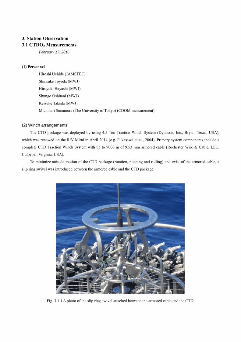
(2) Winch arrangements
The CTD package was deployed by using 4.5 Ton Traction Winch System (Dynacon, Inc., Bryan, Texas, USA),
which was renewed on the R/V Mirai in April 2014 (e.g. Fukasawa et al., 2004). Primary system components include a
complete CTD Traction Winch System with up to 9000 m of 9.53 mm armored cable (Rochester Wire & Cable, LLC,
Culpeper, Virginia, USA).
To minimize attitude motion of the CTD package (rotation, pitching and rolling) and twist of the armored cable, a
slip ring swivel was introduced between the armored cable and the CTD package.
Fig. 3.1.1 A photo of the slip ring swivel attached between the armored cable and the CTD.

--
55
(3) Overview of the equipment
The CTD system was SBE 911plus system (Sea-Bird Electronics, Inc., Bellevue, Washington, USA). The SBE
911plus system controls 36-position SBE 32 Carousel Water Sampler. The Carousel accepts 12-litre Niskin-X water
sample bottles (General Oceanics, Inc., Miami, Florida, USA). The SBE 9plus was mounted horizontally in a
36-position carousel frame. SBE’s temperature (SBE 3) and conductivity (SBE 4) sensor modules were used with
the SBE 9plus underwater unit. The pressure sensor is mounted in the main housing of the underwater unit and is
ported to outside through the oil-filled plastic capillary tube. A modular unit of underwater housing pump (SBE 5T)
flushes water through sensor tubing at a constant rate independent of the CTD’s motion, and pumping rate (3000
rpm) remain nearly constant over the entire input voltage range of 12-18 volts DC. Flow speed of pumped water in
standard TC duct is about 2.4 m/s. Two sets of temperature and conductivity modules were used. An SBE’s
dissolved oxygen sensor (SBE 43) was placed between the primary conductivity sensor and the pump module.
Auxiliary sensors, a Deep Ocean Standards Thermometer (SBE 35), an altimeter (PSA-916T; Teledyne Benthos,
Inc., North Falmous, Massachusetts, USA), an oxygen optodes (RINKO-III; JFE Advantech Co., Ltd, Kobe Hyogo,
Japan), a fluorometers (Seapoint sensors, Inc., Kingston, New Hampshire, USA), a transmissometer (C-Star
Transmissometer; WET Labs, Inc., Philomath, Oregon, USA), a Photosynthetically Active Radiation (PAR) sensor
(Satlantic, LP, Halifax, Nova Scotia, Canada), and a colored dissolved organic matter (ECO FL CDOM, WET Labs,
Inc., Philomath, Oregon, USA) were also used with the SBE 9plus underwater unit. To minimize rotation of the
CTD package, a heavy stainless frame (total weight of the CTD package without sea water in the bottles is about
1000 kg) was used with an aluminum plate (54 × 90 cm).
Summary of the system used in this cruise
36-position Carousel system
Deck unit:
SBE 11plus, S/N 11P54451-0872
Under water unit:
SBE 9plus, S/N 09P38273_74766 (pressure sensor S/N: 0786)
Temperature sensor:
SBE 3plus, S/N 03P4815 (primary)
SBE 3, S/N 031525 (secondary)
Conductivity sensor:
SBE 4, S/N 042435 (primary)
SBE 4, S/N 042854 (secondary)
Oxygen sensor:
SBE 43, S/N 430330
JFE Advantech RINKO-III, S/N 0024 (foil batch no. 144002A)
Pump:
SBE 5T, S/N 054595 (primary)

--
56
SBE 5T, S/N 054598 (secondary)
Altimeter:
PSA-916T, S/N 1157
Deep Ocean Standards Thermometer:
SBE 35, S/N 0022
Fluorometer:
Seapoint Sensors, Inc., S/N 3497 (measurement range: 0-10 µg/L)
Transmissometer:
C-Star, S/N CST-1363DR
PAR:
Satlantic LP, S/N 0049
CDOM:
ECO FL CDOM, S/N FLCDRTD-2014 (measurement range: 0-500 ppb)
Carousel Water Sampler:
SBE 32, S/N 0924
Water sample bottle:
12-litre Niskin-X model 1010X (no TEFLON coating)
(4) Pre-cruise calibration
i. Pressure
The Paroscientific series 4000 Digiquartz high pressure transducer (Model 415K: Paroscientific, Inc., Redmond,
Washington, USA) uses a quartz crystal resonator whose frequency of oscillation varies with pressure induced stress with
0.01 per million of resolution over the absolute pressure range of 0 to 15000 psia (0 to 10332 dbar). Also, a quartz crystal
temperature signal is used to compensate for a wide range of temperature changes at the time of an observation. The
pressure sensor has a nominal accuracy of 0.015 % FS (1.5 dbar), typical stability of 0.0015 % FS/month (0.15
dbar/month), and resolution of 0.001 % FS (0.1 dbar). Since the pressure sensor measures the absolute value, it
inherently includes atmospheric pressure (about 14.7 psi). SEASOFT subtracts 14.7 psi from computed pressure
automatically.
Pre-cruise sensor calibrations for linearization were performed at SBE, Inc. The time drift of the pressure sensor is
adjusted by periodic recertification corrections against a dead-weight piston gauge (Model 480DA, S/N 23906; Piston
unit, S/N 079K; Weight set, S/N 3070; Bundenberg Gauge Co. Ltd., Irlam, Manchester, UK). The corrections are
performed at JAMSTEC, Yokosuka, Kanagawa, Japan by Marine Works Japan Ltd. (MWJ), Yokohama, Kanagawa,
Japan, usually once in a year in order to monitor sensor time drift and linearity.
S/N 0786, 13 July 2015
slope = 0.99980434
offset = –0.13013

--
57
ii. Temperature (SBE 3)
The temperature sensing element is a glass-coated thermistor bead in a stainless steel tube, providing a pressure-free
measurement at depths up to 10500 (6800) m by titanium (aluminum) housing. The SBE 3 thermometer has a nominal
accuracy of 1 mK, typical stability of 0.2 mK/month, and resolution of 0.2 mK at 24 samples per second. The premium
temperature sensor, SBE 3plus, is a more rigorously tested and calibrated version of standard temperature sensor (SBE
3).
Pre-cruise sensor calibrations were performed at SBE, Inc.
S/N 03P4815, 16 April 2015
S/N 031525, 28 July 2015
Pressure sensitivities of SBE 3s were corrected according to a method by Uchida et al. (2007), for the following
sensors.
S/N 03P4815, –3.4597e–7 [°C/dbar]
iii. Conductivity (SBE 4)
The flow-through conductivity sensing element is a glass tube (cell) with three platinum electrodes to provide in-situ
measurements at depths up to 10500 (6800) m by titanium (aluminum) housing. The SBE 4 has a nominal accuracy of
0.0003 S/m, typical stability of 0.0003 S/m/month, and resolution of 0.00004 S/m at 24 samples per second. The
conductivity cells have been replaced to newer style cells for deep ocean measurements.
Pre-cruise sensor calibrations were performed at SBE, Inc.
S/N 042435, 1 May 2015
S/N 042854, 1 May 2014
The value of conductivity at salinity of 35, temperature of 15 °C (IPTS-68) and pressure of 0 dbar is 4.2914 S/m.
iv. Oxygen (SBE 43)
The SBE 43 oxygen sensor uses a Clark polarographic element to provide in-situ measurements at depths up to 7000
m. The range for dissolved oxygen is 120 % of surface saturation in all natural waters, nominal accuracy is 2 % of
saturation, and typical stability is 2 % per 1000 hours.
Pre-cruise sensor calibration was performed at SBE, Inc.
S/N 430330, 10 May 2015
v. Deep Ocean Standards Thermometer
Deep Ocean Standards Thermometer (SBE 35) is an accurate, ocean-range temperature sensor that can be
standardized against Triple Point of Water and Gallium Melt Point cells and is also capable of measuring temperature in
the ocean to depths of 6800 m. The SBE 35 was used to calibrate the SBE 3 temperature sensors in situ (Uchida et al.,
2007).
Pre-cruise sensor linearization was performed at SBE, Inc.
S/N 0022, 4 March 2009

--
58
Then the SBE 35 is certified by measurements in thermodynamic fixed-point cells of the TPW (0.01 °C) and
GaMP (29.7646 °C). The slow time drift of the SBE 35 is adjusted by periodic recertification corrections.
Pre-cruise sensor calibration was performed at SBE, Inc. Since 2014, fixed-point cells traceable to NIST
temperature standards is directly used in the manufacturer’s calibration of the SBE 35 (Uchida et al., 2015).
S/N 0022, 4 February 2015 (slope and offset correction)
Slope = 1.000007
Offset = 0.000246
The time required per sample = 1.1 × NCYCLES + 2.7 seconds. The 1.1 seconds is total time per an acquisition
cycle. NCYCLES is the number of acquisition cycles per sample and was set to 4. The 2.7 seconds is required for
converting the measured values to temperature and storing average in EEPROM.
vi. Altimeter
Benthos PSA-916T Sonar Altimeter (Teledyne Benthos, Inc.) determines the distance of the target from the unit by
generating a narrow beam acoustic pulse and measuring the travel time for the pulse to bounce back from the target
surface. It is rated for operation in water depths up to 10000 m. The PSA-916T uses the nominal speed of sound of 1500
m/s.
vii. Oxygen optode (RINKO)
RINKO (JFE Alec Co., Ltd.) is based on the ability of selected substances to act as dynamic fluorescence quenchers.
RINKO model III is designed to use with a CTD system which accept an auxiliary analog sensor, and is designed to
operate down to 7000 m.
Data from the RINKO can be corrected for the time-dependent, pressure-induced effect by means of the same
method as that developed for the SBE 43 (Edwards et al., 2010). The calibration coefficients, H1 (amplitude of hysteresis
correction), H2 (curvature function for hysteresis), and H3 (time constant for hysteresis) were determined empirically as
follows.
H1 = 0.0055 (for S/N 0024)
H2 = 5000 dbar
H3 = 2000 seconds
Outputs from RINKO are the raw phase shift data. The RINKO can be calibrated by the modified Stern-Volmer
equation slightly modified from a method by Uchida et al. (2010):
O2 (µmol/l) = [(V0 / V)E – 1] / Ksv
where V is voltage, V0 is voltage in the absence of oxygen, Ksv is Stern-Volmer constant. The coefficient E corrects
nonlinearity of the Stern-Volmer equation. The V0 and the Ksv are assumed to be functions of temperature as follows.
Ksv = C0 + C1 × T + C2 × T2
V0 = 1 + C3 × T
V = C4 + C5 × Vb
where T is CTD temperature (°C) and Vb is raw output (volts). V0 and V are normalized by the output in the absence of

--
59
oxygen at 0°C. The oxygen concentration is calculated using accurate temperature data from the CTD temperature sensor
instead of temperature data from the RINKO. The pressure-compensated oxygen concentration O2c can be calculated as
follows.
O2c = O2 (1 + Cpp / 1000)
where p is CTD pressure (dbar) and Cp is the compensation coefficient. Since the sensing foil of the optode is permeable
only to gas and not to water, the optode oxygen must be corrected for salinity. The salinity-compensated oxygen can be
calculated by multiplying the factor of the effect of salt on the oxygen solubility (Garcia and Gordon, 1992).
Pre-cruise sensor calibrations were performed at RCGC/JAMSTEC.
S/N 0024, 10 May 2015
viii. Fluorometer
The Seapoint Chlorophyll Fluorometer (Seapoint Sensors, Inc., Kingston, New Hampshire, USA) provides in-situ
measurements of chlorophyll-a at depths up to 6000 m. The instrument uses modulated blue LED lamps and a blue
excitation filter to excite chlorophyll-a. The fluorescent light emitted by the chlorophyll-a passes through a red emission
filter and is detected by a silicon photodiode. The low level signal is then processed using synchronous demodulation
circuitry, which generates an output voltage proportional to chlorophyll-a concentration.
ix. Transmissometer
The C-Star Transmissometer (WET Labs, Inc., Philomath, Oregon, USA) measures light transmittance at a single
wavelength (650 nm) over a know path (25 cm). In general, losses of light propagating through water can be attributed to
two primary causes: scattering and absorption. By projecting a collimated beam of light through the water and placing a
focused receiver at a known distance away, one can quantify these losses. The ratio of light gathered by the receiver to
the amount originating at the source is known as the beam transmittance. Suspended particles, phytoplankton, bacteria
and dissolved organic matter contribute to the losses sensed by the instrument. Thus, the instrument provides information
both for an indication of the total concentrations of matter in the water as well as for a value of the water clarity.
Light transmission Tr (in %) and beam attenuation coefficient cp are calculated from the sensor output (V in volt) as
follows.
Tr = (c0 + c1 V) × 100
cp = – (1 / 0.25) ln(Tr / 100)
The calibration coefficients were determined by using the data obtained in the R/V Mirai MR15-03 cruise.
x. PAR
Photosynthetically Active Radiation (PAR) sensors (Satlantic, LP, Halifax, Nova Scotia, Canada) provide highly
accurate measurements of PAR (400 – 700 nm) for a wide range of aquatic and terrestrial applications. The ideal spectral
response for a PAR sensor is one that gives equal emphasis to all photons between 400 – 700 nm. Satlantic PAR sensors
use a high quality filtered silicon photodiode to provide a near equal spectral response across the entire wavelength range
of the measurement.

--
60
Pre-cruise sensor calibration was performed at Satlantic, LP.
S/N 0049, 22 January 2009
xi. CDOM
The Environmental Characterization Optics (ECO) miniature fluorometer (WET Labs, Inc., Philomath, Oregon,
USA) allows the user to measure relative Colored Dissolved Organic Matter (CDOM) concentrations by directly
measuring the amount of fluorescence emission in a sample volume of water. The CDOM fluorometer uses an UV LED
to provide the excitation source. An interference filter is used to reject the small amount of out-of-band light emitted by
the LED. The light from the source enters the water volume at an angle of approximately 55-60 degrees with respect to
the end face of the unit. Fluoresced light is received by a detector positioned where the acceptance angle forms a
140-degree intersection with the source beam. An interference filter is used to discriminate against the scattered
excitation light.
CDOM (Quinine Dihydrate Equivalent) concentration expressed in ppb can be derived using the equation as
follows.
CDOM = Scale Factor * (Output – Dark Counts)
Pre-cruise sensor calibration was performed at WET Labs.
S/N FLCDRTD-2014, 1 September 2015
Dark Counts: 0.025 V
Scale Factor: 106 ppb/V
(5) Data collection and processing
i. Data collection
CTD system was powered on at least 20 minutes in advance of the data acquisition to stabilize the pressure sensor
and was powered off at least two minutes after the operation in order to acquire pressure data on the ship’s deck.
The package was lowered into the water from the starboard side and held 10 m beneath the surface in order to
activate the pump. After the pump was activated, the package was lifted to the surface and lowered at a rate of 1.0 m/s to
200 m (or 300 m when significant wave height was high) then the package was stopped to operate the heave compensator
of the crane. The package was lowered again at a rate of 1.2 m/s to the bottom. For the up cast, the package was lifted at
a rate of 1.1 m/s except for bottle firing stops. As a rule, the bottle was fired after waiting from the stop for 30 seconds
and the package was stayed at least 5 seconds for measurement of the SBE 35 at each bottle firing stops. For depths
where vertical gradient of water properties were expected to be large (from surface to thermocline), the bottle was
exceptionally fired after waiting from the stop for 60 seconds to enhance exchanging the water between inside and
outside of the bottle. At 200 m (or 300 m) from the surface, the package was stopped to stop the heave compensator of
the crane.
Water samples were collected using a 36-bottle SBE 32 Carousel Water Sampler with 12-litre Niskin-X bottles.
Before a cast taken water for CFCs, the bottle frame and Niskin-X bottles were wiped with acetone. At station 001_1,
012_1, 022_1, 022_2, 030_1 and 037_1, specially washed Niskin-X bottles were used for #2 and #3, since samples for

--
61
incubation were collected from the bottles.
Data acquisition software
SEASAVE-Win32, version 7.23.2
ii. Data collection problems
(a) Miss trip, miss fire, and remarkable leak
Niskin bottles did not trip correctly at the following stations.
Miss trip Miss fire Leak
none none 007_1 #14 stopcock: O-ring of the stopcock replaced
025_1 #30 stopcock: O-ring of the end closure replaced
033_3 #27 end closure: O-ring of the end closure replaced
(b) Failure of the slip ring swivel
The slip ring swivel failed by sea water immersion from the nipple joints at beginning of station 011_1.
Therefore, the slip ring swivel was detached from the CTD cast.
(d) Cable replacement
Cables for sensors were replaced after the following stations.
900_1: noise of the secondary temperature
010_2: noise of fluorometer
035_1: noise of transmissometer at station 034_1 and 035_1
(e) Noise in down cast data
Secondary conductivity data were noisy at station 043_1 from 698 dbar of down cast due to a jellyfish.
Transmissometer data were noisy at station 016_1 (from 1484 to 2556 dbar), 034_1 (from 539 to 544 dbar), and the
data were removed and linearly interpolated. CDOM data were flagged as 4 (bad measurement) for depths deeper
than about 4500 m due to noise and large shift of the data
iii. Data processing
SEASOFT consists of modular menu driven routines for acquisition, display, processing, and archiving of
oceanographic data acquired with SBE equipment. Raw data are acquired from instruments and are stored as unmodified
data. The conversion module DATCNV uses instrument configuration and calibration coefficients to create a converted
engineering unit data file that is operated on by all SEASOFT post processing modules. The following are the SEASOFT
and original software data processing module sequence and specifications used in the reduction of CTD data in this
cruise.
Data processing software
SBEDataProcessing-Win32, version 7.23.2

--
62
DATCNV converted the raw data to engineering unit data. DATCNV also extracted bottle information where scans
were marked with the bottle confirm bit during acquisition. The duration was set to 4.4 seconds, and the offset was set to
0.0 second. The hysteresis correction for the SBE 43 data (voltage) was applied for both profile and bottle information
data.
TCORP (original module, version 1.1) corrected the pressure sensitivity of the SBE 3 for both profile and bottle
information data.
RINKOCOR (original module, version 1.0) corrected the time-dependent, pressure-induced effect (hysteresis) of the
RINKO for both profile data.
RINKOCORROS (original module, version 1.0) corrected the time-dependent, pressure-induced effect (hysteresis)
of the RINKO for bottle information data by using the hysteresis-corrected profile data.
BOTTLESUM created a summary of the bottle data. The data were averaged over 4.4 seconds.
ALIGNCTD converted the time-sequence of sensor outputs into the pressure sequence to ensure that all calculations
were made using measurements from the same parcel of water. For a SBE 9plus CTD with the ducted temperature and
conductivity sensors and a 3000-rpm pump, the typical net advance of the conductivity relative to the temperature is
0.073 seconds. So, the SBE 11plus deck unit was set to advance the primary and the secondary conductivity for 1.73
scans (1.75/24 = 0.073 seconds). Oxygen data are also systematically delayed with respect to depth mainly because of the
long time constant of the oxygen sensor and of an additional delay from the transit time of water in the pumped plumbing
line. This delay was compensated by 5 seconds advancing the SBE 43 oxygen sensor output (voltage) relative to the
temperature data. Delay of the RINKO data was also compensated by 1 second advancing sensor output (voltage) relative
to the temperature data. Delay of the transmissometer data was also compensated by 2 seconds advancing sensor output
(voltage) relative to the temperature data.
WILDEDIT marked extreme outliers in the data files. The first pass of WILDEDIT obtained an accurate
estimate of the true standard deviation of the data. The data were read in blocks of 1000 scans. Data greater than 10
standard deviations were flagged. The second pass computed a standard deviation over the same 1000 scans
excluding the flagged values. Values greater than 20 standard deviations were marked bad. This process was
applied to pressure, temperature, conductivity, and SBE 43 output.
CELLTM used a recursive filter to remove conductivity cell thermal mass effects from the measured conductivity.
Typical values used were thermal anomaly amplitude alpha = 0.03 and the time constant 1/beta = 7.0.
FILTER performed a low pass filter on pressure with a time constant of 0.15 seconds. In order to produce zero phase
lag (no time shift) the filter runs forward first then backwards.
WFILTER performed as a median filter to remove spikes in fluorometer, transmissometer, and CDOM data. A
median value was determined by 49 scans of the window. For CDOM data, an additional box-car filter with a window of
361 scans was applied to remove noise.
SECTIONU (original module, version 1.1) selected a time span of data based on scan number in order to reduce a
file size. The minimum number was set to be the start time when the CTD package was beneath the sea-surface after
activation of the pump. The maximum number was set to be the end time when the depth of the package was 1 dbar
below the surface. The minimum and maximum numbers were automatically calculated in the module.

--
63
LOOPEDIT marked scans where the CTD was moving less than the minimum velocity of 0.0 m/s (traveling
backwards due to ship roll).
DESPIKE (original module, version 1.0) removed spikes of the data. A median and mean absolute deviation was
calculated in 1-dbar pressure bins for both down- and up-cast, excluding the flagged values. Values greater than 4 mean
absolute deviations from the median were marked bad for each bin. This process was performed 2 times for temperature,
conductivity, SBE 43, and RINKO output.
DERIVE was used to compute oxygen (SBE 43).
BINAVG averaged the data into 1-dbar pressure bins. The center value of the first bin was set equal to the bin size.
The bin minimum and maximum values are the center value plus and minus half the bin size. Scans with pressures
greater than the minimum and less than or equal to the maximum were averaged. Scans were interpolated so that a data
record exist every dbar.
BOTTOMCUT (original module, version 0.1) deleted the deepest pressure bin when the averaged scan number of
the deepest bin was smaller than the average scan number of the bin just above.
DERIVE was re-used to compute salinity, potential temperature, and density (σθ).
SPLIT was used to split data into the down cast and the up cast.
Remaining spikes in the CTD data were manually eliminated from the 1-dbar-averaged data. The data gaps resulting
from the elimination were linearly interpolated with a quality flag of 6.
(6) Post-cruise calibration
i. Pressure
The CTD pressure sensor offset in the period of the cruise was estimated from the pressure readings on the ship deck.
For best results the Paroscientific sensor was powered on for at least 20 minutes before the operation. In order to get the
calibration data for the pre- and post-cast pressure sensor drift, the CTD deck pressure was averaged over first and last
one minute, respectively. Then the atmospheric pressure deviation from a standard atmospheric pressure (14.7 psi) was
subtracted from the CTD deck pressure to check the pressure sensor time drift. The atmospheric pressure was measured
at the captain deck (20 m high from the base line) and sub-sampled one-minute interval as a meteorological data.
The pre- and the post-casts deck pressure data showed temperature dependency for the pressure sensor (Fig. 3.1.2).
To correct the temperature dependency, the manufacturer’s calibration coefficients were slightly modified on board as
follows:
T1 = 29.88499
T2 = –2.565740e–4
T3 = 4.799030e–6
Offset = 0.0
Time series of the CTD deck pressure is shown in Fig. 3.1.3. The CTD pressure sensor offset was estimated from the
deck pressure. Mean of the pre- and the post-casts data over the whole period gave an estimation of the pressure sensor
offset (–0.01 dbar) from the pre-cruise calibration. The post-cruise correction of the pressure data is not deemed
necessary for the pressure sensor.

--
64
Fig. 3.1.2 Pre- and post-casts CTD deck pressure. Atmospheric pressure deviation from a standard atmospheric pressure
was subtracted from the CTD deck pressure. Black dots show the original data and red dots show the data corrected
for the temperature dependency of the sensor.
Fig. 3.1.3 Time series of the CTD deck pressure. Atmospheric pressure deviation (magenta dots) from a standard
atmospheric pressure was subtracted from the CTD deck pressure. Blue and green dots indicate pre- and post-cast
deck pressures, respectively. Red dots indicate averages of the pre- and the post-cast deck pressures.

--
65
ii. Temperature
The CTD temperature sensors (SBE 3) were calibrated with the SBE 35 under the assumption that discrepancies
between SBE 3 and SBE 35 data were due to pressure sensitivity, the viscous heating effect, and time drift of the SBE 3,
according to a method by Uchida et al. (2007).
Post-cruise sensor calibration for the SBE 35 will be performed at SBE, Inc in 2016
The CTD temperature was preliminary calibrated as
Calibrated temperature = T – (c0 × P + c1 × t + c2 )
where T is CTD temperature in °C, P is pressure in dbar, t is time in days from pre-cruise calibration date of the CTD
temperature and c0, c1, and c2 are calibration coefficients. The coefficients were determined using the data for the depths
deeper than 1950 dbar. The coefficient c1 was set to zero for this cruise.
The primary temperature data were basically used for the post-cruise calibration. The secondary temperature sensor
was also calibrated and used instead of the primary temperature data when the data quality of the primary temperature
data was bad. The calibration coefficients are listed in Table 3.1.1. The results of the post-cruise calibration for the CTD
temperature are summarized in Table 3.1.2 and shown in Fig. 3.1.4.
Table 3.1.1 Calibration coefficients for the CTD temperature sensors.
==========================================================================
Serial number c0 (°C/dbar) c1 (°C/day) c2 (°C)
-----------------------------------------------------------------------------------------------------------------------------
3P4815 –4.79962e–8 0.0 –0.0007
-----------------------------------------------------------------------------------------------------------------------------
Table 3.1.2 Difference between the CTD temperature and the SBE 35 after the post-cruise calibration. Mean and standard
deviation (Sdev) are calculated for the data below and above 1950 dbar. Number of data used is also shown.
==========================================================================
Serial Pressure ≥ 1950 dbar Pressure < 1950 dbar
number ------------------------------------------ -----------------------------------------------
Number Mean Sdev Number Mean Sdev
(mK) (mK) (mK) (mK)
------------------------------------------------------------------------------------------------------------------------------
3P4815 467 0.0 0.2 854 –0.0 6.8
------------------------------------------------------------------------------------------------------------------------------

--
66
Fig. 3.1.4 Difference between the CTD temperature (primary) and the SBE 35. Blue and red dots indicate before and
after the post-cruise calibration using the SBE 35 data, respectively. Lower two panels show histogram of the
difference after the calibration.

--
67
iii. Salinity
The discrepancy between the CTD conductivity and the conductivity calculated from the bottle salinity data with the
CTD temperature and pressure data is considered to be a function of conductivity, pressure and time. The CTD
conductivity was calibrated as
Calibrated conductivity = c0 × C + c1 × P + c2 × C × P + c3 × C2 + c4 × t + c5
where C is CTD conductivity in S/m, P is pressure in dbar, t is time in days, and c0, c1, c2, c3, c4 and c5 are calibration
coefficients. The best fit sets of coefficients were determined by a least square technique to minimize the deviation from
the conductivity calculated from the bottle salinity data. The coefficient c4 was set to zero for this cruise.
The primary conductivity data created by the software module ROSSUM were used after the post-cruise
calibration for the temperature data. The calibration coefficients are listed in Table 3.1.3. The results of the
post-cruise calibration for the CTD salinity are summarized in Table 3.1.4 and shown in Fig. 3.1.5.
Table 3.1.3 Calibration coefficients for the CTD conductivity sensors.
==========================================================================
Serial c0 c1 c2 c3 c4
Number [S/(m dbar)] (1/dbar) [1/(S/m)] (S/m)
-----------------------------------------------------------------------------------------------------------------------------
042435 –1.51687e–4 1.09232e–7 –3.67361e–8 4.72348e–12 5.09192e–4
-----------------------------------------------------------------------------------------------------------------------------
Table 3.1.4 Difference between the CTD salinity and the bottle salinity after the post-cruise calibration. Mean and
standard deviation (Sdev) (in 10–3) are calculated for the data below and above 1950 dbar. Number of data used is
also shown.
==========================================================================
Serial Pressure ≥ 1950 dbar Pressure < 1950 dbar
number ------------------------------------------ -----------------------------------------------
Number Mean Sdev Number Mean Sdev
------------------------------------------------------------------------------------------------------------------------------
042435 493 –0.0 0.4 861 0.2 4.5
------------------------------------------------------------------------------------------------------------------------------

--
68
Fig. 3.1.5 Difference between the CTD salinity (primary) and the bottle salinity. Blue and red dots indicate before and
after the post-cruise calibration, respectively. Lower two panels show histogram of the difference after the
calibration.
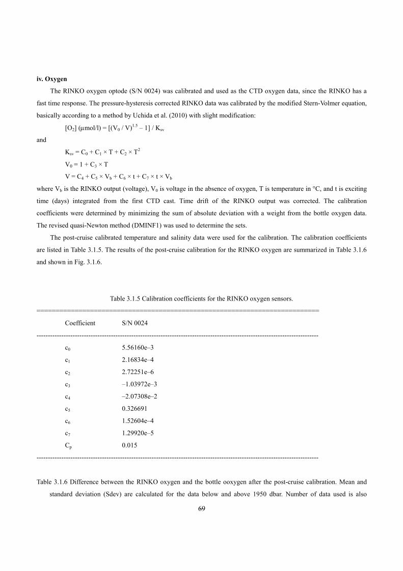
--
69
iv. Oxygen
The RINKO oxygen optode (S/N 0024) was calibrated and used as the CTD oxygen data, since the RINKO has a
fast time response. The pressure-hysteresis corrected RINKO data was calibrated by the modified Stern-Volmer equation,
basically according to a method by Uchida et al. (2010) with slight modification:
[O2] (µmol/l) = [(V0 / V)1.5 – 1] / Ksv
and
Ksv = C0 + C1 × T + C2 × T2
V0 = 1 + C3 × T
V = C4 + C5 × Vb + C6 × t + C7 × t × Vb
where Vb is the RINKO output (voltage), V0 is voltage in the absence of oxygen, T is temperature in °C, and t is exciting
time (days) integrated from the first CTD cast. Time drift of the RINKO output was corrected. The calibration
coefficients were determined by minimizing the sum of absolute deviation with a weight from the bottle oxygen data.
The revised quasi-Newton method (DMINF1) was used to determine the sets.
The post-cruise calibrated temperature and salinity data were used for the calibration. The calibration coefficients
are listed in Table 3.1.5. The results of the post-cruise calibration for the RINKO oxygen are summarized in Table 3.1.6
and shown in Fig. 3.1.6.
Table 3.1.5 Calibration coefficients for the RINKO oxygen sensors.
==========================================================================
Coefficient S/N 0024
-----------------------------------------------------------------------------------------------------------------------------
c0 5.56160e–3
c1 2.16834e–4
c2 2.72251e–6
c3 –1.03972e–3
c4 –2.07308e–2
c5 0.326691
c6 1.52604e–4
c7 1.29920e–5
Cp 0.015
-----------------------------------------------------------------------------------------------------------------------------
Table 3.1.6 Difference between the RINKO oxygen and the bottle ooxygen after the post-cruise calibration. Mean and
standard deviation (Sdev) are calculated for the data below and above 1950 dbar. Number of data used is also

--
70
shown.
==========================================================================
Serial Pressure ≥ 1950 dbar Pressure < 1950 dbar
number ------------------------------------------ -----------------------------------------------
Number Mean Sdev Number Mean Sdev
[µmol/kg] [µmol/kg]
------------------------------------------------------------------------------------------------------------------------------
0024 502 0.11 0.39 859 0.02 0.57
------------------------------------------------------------------------------------------------------------------------------

--
71
Fig. 3.1.6 Difference between the CTD oxygen and the bottle oxygen. Blue and red dots indicate before and after the
post-cruise calibration, respectively. Lower two panels show histogram of the difference after the calibration.
v. Fluorometer

--
72
The CTD fluorometer (FLUOR in µg/L) was calibrated by comparing with the bottle sampled chlorophyll-a as
FLUORc = c0 + c1 × FLUOR
where c0 and c1 are calibration coefficients. The CTD fluorometer data is slightly noisy so that the up cast profile data
which was averaged over one decibar agree with the bottle sampled data better than the discrete CTD fluorometer data
obtained at bottle-firing stop. Therefore, the CTD fluorometer data at water sampling depths extracted from the up cast
profile data were compared with the bottle sampled chlorophyll-a data. The bottle sampled data obtained at dark
condition [PAR (Photosynthetically Available Radiation) < 50 µE/(m2 sec)] were used for the calibration, since
sensitivity of the fluorometer to chlorophyll a is different at nighttime and daytime (Section 2.4 in Uchida et al., 2015)
(Fig. 3.1.7). The calibration coefficients are listed in Table 3.1.7. The results of the post-cruise calibration for the
fluorometer are summarized in Table 3.1.8 and shown in Fig. 3.1.8.
Fig. 3.1.7. Comparison of the CTD fluorometer and the bottle sampled chlorophyll-a. The regression lines are also
shown.
Table 3.1.7. Calibration coefficients for the CTD fluorometer.
==========================================================================
c0 c1 Note
-----------------------------------------------------------------------------------------------------------------------------
–2.35932e–3 0.689112
-----------------------------------------------------------------------------------------------------------------------------

--
73
Table 3.1.8. Difference between the CTD fluorometer and the bottle chlorophyll-a after the post-cruise calibration. Mean,
standard deviation (Sdev), and number of data used are shown. Data obtained at daytime are also used in this calculation.
==========================================================================
Number Mean Sdev
-----------------------------------------------------------------------------------------------------------------------------
156 –0.00 µg/L 0.07 µg/L
----------------------------------------------------------------------------------------------------------------------------
Fig. 3.1.8. Comparison of the CTD fluorometer and the bottle sampled chlorophyll-a. Blue and red dots indicate before
and after the post-cruise calibration, respectively. Lower panel shows histogram of the difference after the
calibration. Data obtained at daytime are also shown in this figure.

--
74
vi. Transmissometer
The transmissometer (Tr in %) is calibrated as
Tr = (V–Vd) / (Vr–Vd) × 100
wehre V is the measured signal (voltage), Vd is the dark offset for the instrument, and Vr is the signal for clear water. Vd
can be obtained by blocking the light path. Vd and Vair, which is the signal for air, were measured on deck before each
cast after wiping the optical windows with ethanol. Vd was constant (0.0012) during the cruise. Vr is estimated from the
measured maximum signal in the deep ocean at each cast. Since the transmissometer drifted in time (Fig. 3.1.9), Vr is
expressed as
Vr = c0 + c1×t + c2×t2
where t is working time (in days) of the transmissometer, and c0, c1, and c2 are calibration coefficients.
Maximum signal was extracted for each cast (Fig. 3.1.9). Data whose depth of the maximum signal was
shallower than 200 dbar were not used to estimate Vr (black dots in Fig. 3.1.9). Fits were made iteratively,
removing negatively deviated outliers (red dots in Fig. 3.1.9) greater than 2 standard deviations until no more
outliers remain. The calibration coefficients thus determined are listed in Table 3.1.9. The coefficient c2 was set to
zero for this cruise.
Fig. 3.1.9. Time series of an output signal (voltage) from transmissometer at deep ocean (Vdeep). The black solid line
indicates the modeled signal in the deep clear ocean. Black and red dots were not used to estimate the final calibration
coefficients (see text for detail).
Table 3.1.9 Calibration coefficients for the CTD transmissometer.

--
75
==========================================================================
Leg c0 c1 Vd
-----------------------------------------------------------------------------------------------------------------------------
1 4.61740 –2.94693e–3 0.0012
-----------------------------------------------------------------------------------------------------------------------------
vii. PAR
The PAR sensor was calibrated with an offset correction. The offset was estimated from the data measured in the
deep ocean during the cruise. The corrected data (PARc) is calculated from the raw data (PAR) as follows:
PARc [µE m–2 s–1] = PAR – 0.046.
vii. CDOM
The CDOM sensor wasn’t calibrated, since the reference data (see Section 3.9) was not adequate for the in-situ
calibration. The data were low-pass filtered by a running mean with a window of 15 seconds (about 13 m) in the data
processing mentioned above, since the data was noisy.
(7) References
Edwards, B., D. Murphy, C. Janzen and N. Larson (2010): Calibration, response, and hysteresis in deep-sea dissolved
oxygen measurements, J. Atmos. Oceanic Technol., 27, 920–931.
Fukasawa, M., T. Kawano and H. Uchida (2004): Blue Earth Global Expedition collects CTD data aboard Mirai,
BEAGLE 2003 conducted using a Dynacon CTD traction winch and motion-compensated crane, Sea Technology, 45,
14–18.
García, H. E. and L. I. Gordon (1992): Oxygen solubility in seawater: Better fitting equations. Limnol. Oceanogr., 37 (6),
1307–1312.
Uchida, H., G. C. Johnson, and K. E. McTaggart (2010): CTD oxygen sensor calibration procedures, The GO-SHIP
Repeat Hydrography Manual: A collection of expert reports and guidelines, IOCCP Rep., No. 14, ICPO Pub. Ser.
No. 134.
Uchida, H., K. Katsumata, and T. Doi (2015): WHP P14S, S04I Revisit Data Book, JASTEC, Yokosuka, 187 pp.
Uchida, H., T. Nakano, J. Tamba, J. V. Widiatmo, K. Yamazawa, S. Ozawa and T. Kawano (2015): Deep ocean
temperature measurement with an uncertainty of 0.7 mK, J. Atmos. Oceanic Technol., 32, 2199–2210.
Uchida, H., K. Ohyama, S. Ozawa, and M. Fukasawa (2007): In situ calibration of the Sea-Bird 9plus CTD thermometer,
J. Atmos. Oceanic Technol., 24, 1961–1967.
--
76
3.2 Bottle Salinity January 27, 2016
(1) Personnel
Hiroshi Uchida (JAMSTEC)
Sonoka Wakatsuki (MWJ)
Hiroki Ushiromura (MWJ)
(2) Objectives
Bottle salinities were measured to calibrate CTD salinity data.
(3) Instrument and Method
Salinity measurement was conducted basically based on a method by Kawano (2010).
i. Salinity Sample Collection
The bottles in which the salinity samples were collected and stored were 250 ml brown borosilicate glass bottles
with screw caps (PTFE packing). Each bottle was rinsed three times with sample water and was filled to the shoulder of
the bottle. The caps were also thoroughly rinsed. Salinity samples were stored more than 24 hours in the same laboratory
as the salinity measurement was made.
ii. Instruments and Methods
Salinity of water samples was measured with a salinometer (Autosal model 8400B; Guildline Instruments Ltd.,
Ontario, Canada; S/N 62556), which was modified by adding an peristaltic-type intake pump (Ocean Scientific
International Ltd., Hampshire, UK) and two platinum thermometers (Guildline Instruments Ltd., model 9450). One
thermometer monitored an ambient temperature and the other monitored a salinometer’s bath temperature. The resolution
of the thermometers was 0.001 °C. The measurement system was almost same as Aoyama et al. (2002). The salinometer
was operated in the air-conditioned laboratory of the ship at a bath temperature of 24 °C.
The ambient temperature varied from approximately 22.3 to 24.3 °C, while the bath temperature was stable and
varied within ±0.006 °C. A measure of a double conductivity ratio of a sample was taken as a median of 31 readings.
Data collection was started after 10 seconds and it took about 10 seconds to collect 31 readings by a personal computer.
Data were sampled for the sixth and seventh filling of the cell. In case where the difference between the double
conductivity ratio of this two fillings was smaller than 0.00002, the average value of the two double conductivity ratios
was used to calculate the bottle salinity with the algorithm for practical salinity scale, 1978 (UNESCO, 1981). When the
difference was greater than or equal to the 0.00003, we measured another additional filling of the cell. In case where the
double conductivity ratio of the additional filling did not satisfy the criteria above, we measured other additional fillings
of the cell within 10 fillings in total. In case where the number of fillings was 10 and those fillings did not satisfy the
criteria above, the median of the double conductivity ratios of five fillings were used to calculate the bottle salinity.

--
77
The measurement was conducted about from 2 to 19 hours per day and the cell was cleaned with soap (50 times
diluted solution of S-CLEAN WO-23 [Neutral], Sasaki Chemical Co. Ltd., Kyoto, Japan) after the measurement for each
day. A total of 1672 water samples were measured during the cruise.
(4) Results
i. Standard Seawater
Standardization control was set to 715. The value of STANDBY was 5216±0001 and that of ZERO was 0.00000
or ±0.00001. We used IAPSO Standard Seawater batch P157 whose conductivity ratio is 0.99985 (double conductivity
ratio is 1.99970) as the standard for salinity measurement. We measured 66 bottles of the Standard Seawater during the
cruise. History of double conductivity ratio measurement of the Standard Seawater is shown in Fig. 3.2.1.
Time drift of the salinometer was corrected by using the Standard Seawater measurements. Linear time drift of the
salinometer was estimated from the Standard Seawater measurement by using the least square method (thin black line in
Fig. 3.2.1). No remarkable time drift was estimated from the Standard Seawater measurement. The average of double
conductivity ratio was 1.99968 and the standard deviation was 0.00001, which is equivalent to 0.0002 in salinity.
Fig. 3.2.1. History of double conductivity ratio measurement of the Standard Seawater (P157). Horizontal and vertical
axes represents date and double conductivity ratio, respectively. Red dots indicate raw data and blue dots indicate
corrected data.
ii. Sub-Standard Seawater
We also used sub-standard seawater which was deep-sea water filtered by pore size of 0.45 µm and stored in a 20
liter cubitainer made of polyethylene and stirred for at least 24 hours before measuring. It was measured every 6-8
samples in order to check the possible sudden drift of the salinometer. During the whole measurements, there was no
detectable sudden drift of the salinometer.
iii. Replicate Samples

--
78
We took 257 pairs of replicate samples collected from the same Niskin bottle. Histogram of the absolute difference
between replicate samples is shown in Fig. 3.2.2. The root-mean-square for 256 pairs of replicate samples which are
acceptable-quality data was 0.0002.
Fig. 3.2.2. Histogram of the absolute difference between replicate samples. Horizontal axis is absolute difference in
salinity and vertical axis is frequency.
iv. Duplicate Samples
In this cruise, we took 36 samples collected from the different Niskin bottles at same depth (2000 dbar) of station
900, instead of taking duplicate samples. The average of salinity with the standard deviation was 34.7300 ± 0.0002.
(5) References
Aoyama, M., T. Joyce, T. Kawano and Y. Takatsuki (2002): Standard seawater comparison up to P129. Deep-Sea
Research, I, Vol. 49, 1103-1114.
Kawano (2010): Salinity. The GO-SHIP Repeat Hydrography Manual: A collection of Expert Reports and Guidelines,
IOCCP Report No. 14, ICPO Publication Series No. 134, Version 1.
UNESCO (1981): Tenth report of the Joint Panel on Oceanographic Tables and Standards. UNESCO Tech. Papers in
Mar. Sci., 36, 25 pp.
--
79
3.3 Density February 18, 2016
(1) Personnel
Hiroshi Uchida (JAMSTEC)
(2) Objectives
The objective of this study is to collect absolute salinity (also called “density salinity”) data, and to evaluate an
algorithm to estimate absolute salinity provided along with TEOS-10 (the International Thermodynamic Equation of
Seawater 2010) (IOC et al., 2010).
(3) Materials and methods Seawater densities were measured during the cruise with an oscillation-type density meter (DMA 5000M, serial no.
80570578, Anton-Paar GmbH, Graz, Austria) with a sample changer (Xsample 122, serial no. 80548492, Anton-Paar GmbH). The sample changer was used to load samples automatically from up to ninety-six 12-mL glass vials.
The water samples were collected in 100-mL aluminum bottles (Mini Bottle Can, Daiwa Can Company, Japan). The bottles were stored at room temperature (~23 ºC) upside down usually for 12 to 24 hours to make the temperature of the sample equal to the room temperature. The water sample was filled in a 12-mL glass vial and the glass vial was sealed with Parafilm M (Pechiney Plastic Packaging, Inc., Menasha, Wisconsin, USA) immediately after filling. Densities of the samples were measured at 20 ºC by the density meter two times for each bottle and averaged to estimate the density. When the difference between the two measurements was greater than 0.002, additional measurements were conducted until two samples satisfying the above criteria were obtained.
Time drift of the density meter was monitored by periodically measuring the density of ultra-pure water (Milli-Q water, Millipore, Billerica, Massachusetts, USA) prepared from Yokosuka (Japan) tap water in October 2012. The true density at 20 ºC of the Milli-Q water was estimated to be 998.2042 kg m–3 from the isotopic composition (δD = –8.76 ‰, δ18O = –56.86 ‰) and International Association for the Properties of Water and Steam (IAPWS)-95 standard. An offset correction was applied to the measured density by using the Milli-Q water measurements (ρMilli-Q) with a slight modification of the density dependency (Uchida et al., 2011). The offset (ρoffset) of the measured density (ρ) was reevaluated in November 2014 as follows:
ρoffset = (ρMilli-Q – 998.2042) – (ρ – 998.2042) × 0.000411 [kg m–3]. The offset correction was verified by measuring Reference Material for Density in Seawater (prototype Dn-RM1) developing with Marine Works Japan, Ltd., Kanagawa, Japan, and produced by Kanso Technos Co., Ltd., Osaka, Japan, along with the Milli-Q water.
Density salinity can be back calculated from measured density and temperature (20 ºC) with TEOS-10.
(4) Results
Results of density measurements of the Reference Material for Density in Seawater (Dn-RM1) were shown in Table
3.3.1.
A total of 32 pairs of replicate samples were measured. The root-mean square of the absolute difference of replicate
samples was 0.0009 g/kg.
The measured density salinity anomalies (δSA) are shown in Fig. 3.3.1. The measured δSA well agree with
calculated δSA from Pawlowicz et al. (2011) which exploits the correlation between δSA and nutrient concentrations and

--
80
carbonate system parameters based on mathematical investigation using a model relating composition, conductivity and
density of arbitrary seawaters.
(5) References
IOC, SCOR and IAPSO (2010): The international thermodynamic equation of seawater – 2010: Calculation and use of
thermodynamic properties. Intergovernmental Oceanographic Commission, Manuals and Guides No. 56, United
Nations Educational, Scientific and Cultural Organization (English), 196 pp.
Pawlowicz, R., D. G. Wright and F. J. Millero (2011): The effects of biogeochemical processes on ocean
conductivity/salinity/density relationships and the characterization of real seawater. Ocean Science, 7, 363–387.
Uchida, H., T. Kawano, M. Aoyama and A. Murata (2011): Absolute salinity measurements of standard seawaters for
conductivity and nutrients. La mer, 49, 237–244.
Table 3.3.1. Result of density measurements of the Reference Material for Density in Seawater (prototype Dn-RM1).
==========================================================================
Date Stations Mean density of Note
Dn-RM1 (kg/m3)
------------------------------------------------------------------------------------------------------------------------------
2015/12/29 1,2,3,4,6,10 1024.2631
2015/12/31 14 1024.2637
2016/01/01 18 1024.2628
2016/01/02 22 1024.2627
2016/01/03 26 1024.2631
2016/01/04 31 1024.2619
33 1024.2622
2016/01/06 37 1024.2638
2016/01/07 41 1024.2634
42 1024.2624
2016/01/08 43 1024.2597
45 1024.2601
2016/01/08 46,47 1024.2609
48,50 1024.2602
2016/01/09 51,52 1024.2640
Average: 1024.2623 ± 0.0014
------------------------------------------------------------------------------------------------------------------------------

--
81
Figure 3.3.1. Vertical distribution of density salinity anomaly measured by the density meter. Absolute Salinity anomaly
estimated from nutrients and carbonate parameters (Pawlowicz et al., 2011) are also shown for comparison.
--
82
3.4 Oxygen January 27, 2016
Yuichiro Kumamoto
Japan Agency for Marine-Earth Science and Technology
(1) Personnel
Yuichiro Kumamoto 1), Misato Kuwahara 2), Keitaro Matsumoto 2), Masahiro Orui 2), and Haruka Tamada 2)
1) Japan Agency for Marine-Earth Science and Technology
2) Marine Works Japan Co. Ltd
(2) Objectives
Dissolved oxygen is one of good tracers for the ocean circulation. Climate models predict a decline in oceanic
dissolved oxygen concentration and a consequent expansion of the oxygen minimum layers under global warming
conditions, which results mainly from decreased interior advection and ongoing oxygen consumption by remineralization.
The mechanism of the decrease, however, is still unknown. During MR15-05 cruise, we measured dissolved oxygen
concentration from surface to bottom layers at all the hydrocast stations in the eastern Indian Ocean. All the stations
reoccupied the WOCE Hydrographic Program I10 stations in 1995. Our purpose is to evaluate temporal change in
dissolved oxygen concentration in the North Pacific Ocean during the past decades.
(3) Reagents
Pickling Reagent I: Manganous chloride solution (3M)
Pickling Reagent II: Sodium hydroxide (8M) / sodium iodide solution (4M)
Sulfuric acid solution (5M)
Sodium thiosulfate (0.025M)
Potassium iodate (0.001667M): NMIJ CRM 3006-a No.028, Mass fraction: 99.973 ± 0.018 % (expanded uncertainty)
CSK standard of potassium iodate: Lot KPG6393, Wako Pure Chemical Industries Ltd., 0.0100N
(4) Instruments
Burette for sodium thiosulfate and potassium iodate;
APB-620 and APB-510 manufactured by Kyoto Electronic Co. Ltd. / 10 cm3 of titration vessel
Detector;
Automatic photometric titrator, DOT-01X manufactured by Kimoto Electronic Co. Ltd.
(5) Seawater sampling
Following procedure is based on a determination method in the WHP Operations Manual (Dickson, 1996). Seawater
samples were collected from 12-liters Niskin sampler bottles attached to the CTD-system. Seawater for bottle oxygen
measurement was transferred from the Niskin sampler bottle to a volume calibrated glass flask (ca. 100 cm3). Three times

--
83
volume of the flask of seawater was overflowed. Sample temperature was measured using a thermometer. Then two
reagent solutions (Reagent I, II) of 0.5 cm3 each were added immediately into the sample flask and the stopper was
inserted carefully into the flask. The sample flask was then shaken vigorously to mix the contents and to disperse the
precipitate finely throughout. After the precipitate has settled at least halfway down the flask, the flask was shaken again
to disperse the precipitate. The sample flasks containing pickled samples were stored in a laboratory until they were
titrated.
(6) Sample measurement
At least two hours after the re-shaking, the pickled samples were measured on board. A magnetic stirrer bar and 1 cm3
sulfuric acid solution were added into the sample flask and stirring began. Samples were titrated by sodium thiosulfate
solution whose molarity was determined by potassium iodate solution. Temperature of sodium thiosulfate during titration
was recorded by a thermometer. We measured dissolved oxygen concentration using two sets of the titration apparatus,
named DOT-6 and DOT-8. Dissolved oxygen concentration (µmol kg-1) was calculated by the sample temperature during
the sampling, CTD salinity, flask volume, and titrated volume of the sodium thiosulfate solution.
(7) Standardization
Concentration of sodium thiosulfate titrant (ca. 0.025M) was determined by potassium iodate solution. Pure potassium
iodate was dried in an oven at 130°C. 1.7835 g potassium iodate weighed out accurately was dissolved in deionized
water and diluted to final volume of 5 dm3 in a calibrated volumetric flask (0.001667M). 10 cm3 of the standard
potassium iodate solution was added to a flask using a volume-calibrated dispenser. Then 90 cm3 of deionized water, 1
cm3 of sulfuric acid solution, and 0.5 cm3 of pickling reagent solution II and I were added into the flask in order. Amount
of titrated volume of sodium thiosulfate (usually 5 times measurements average) gave the molarity of the sodium
thiosulfate titrant. Table 3.4.1 shows result of the standardization during this cruise. Coefficient of variation (C.V.) for the
standardizations was 0.016 ± 0.005 % (standard deviation, n = 16), c.a. 0.05 µmol kg-1.
(8) Determination of the blank
The oxygen in the pickling reagents I (0.5 cm3) and II (0.5 cm3) was assumed to be 3.8 × 10⁻⁸ mol (Murray et al.,
1968). The blank from the presence of redox species apart from oxygen in the reagents (the pickling reagents I, II, and
the sulfuric acid solution) was determined as follows. 1 and 2 cm3 of the standard potassium iodate solution were added
to two flasks respectively. Then 100 cm3 of deionized water, 1 cm3 of sulfuric acid solution, and 0.5 cm3 of pickling
reagent solution II and I each were added into the two flasks in order. The blank was determined by difference between
the two times of the first (1 cm3 of KIO3) titrated volume of the sodium thiosulfate and the second (2 cm3 of KIO3) one.
The results of 3 times blank determinations were averaged (Table 3.4.1). The averaged blank values for DOT-6 and
DOT-8 were 0.002 ± 0.002 (standard deviation, n=8) and 0.000 ± 0.002 (standard deviation, n=8) cm3, respectively.

--
84
Table 3.4.1 Results of the standardization (End point, E.P.) and the blank determinations (cm3).
(9) Replicate sample measurement
From a routine CTD cast at all the stations, a pair of replicate samples was collected at four layers of 50, 400, 1800,
and 3500 dbars. The total number of the replicate sample pairs in good measurement (flagged 2) was 170 (Fig. 3.4.1).
The standard deviation of the replicate measurement was 0.60 µmol kg-1 calculated by a procedure (SOP23) in DOE
(1994).
Figure 3.4.1 Oxygen difference between measurements of a replicate pair against oxygen concentration.
Date
(UTC) KIO3 No.
Na2S2O3
No.
DOT-6 DOT-8 Stations
E.P. blank E.P. blank
2015/12/27 K1504E02 T1505A 3.962 0.002 3.963 0.000 001-015
2015/12/30 K1504E03 T1505A 3.965 0.003 3.965 0.001 016-026
2016/01/03 K1504E04 T1505B 3.957 0.000 3.959 0.001 027-041
2016/01/06 K1504E05 T1505B 3.957 0.002 3.958 0.000 042-052
Duplicated
Niskin # Niskin Pres.(db)
Oxygen
(µmol kg-1)
1 X12J01 2000 139.67
2 X12J02 2000 139.74
3 X12J03 2001 139.73
4 X12104 2001 139.91
5 X12J05 2000 139.78
6 X12J06 2000 139.91

--
85
7 X12J07 2000 139.85
8 X12J08 2000 139.93
9 X12J09 2000 139.87
10 X12J10 2000 139.85
11 X12J11 2001 139.96
12 X12J12 2001 139.87
13 X12J13 2001 140.02
14 X12J14 2001 139.86
15 X12J15 2001 139.89
16 X12J16 2001 139.92
17 X12J17 2000 139.97
18 X12J18 1999 139.86
19 X12J19 2000 139.97
20 X12J20 1999 139.99
21 X12J21 2000 139.94
22 X12J22 2001 139.90
23 X12J23 2001 139.97
24 X12J24 2001 139.98
25 X12J25 2000 139.91
26 X12J26 2001 139.94
27 X12J27 2000 139.93
28 X12J28 2001 139.70
29 X12J29 2001 139.89
30 X12J30 2001 139.78
31 X12J31 2001 139.88
32 X12J32 2001 139.79
33 X12J33 2001 140.02
34 X12J34 2001 139.92
35 X12J35 2000 139.77
36 X12J36 2000 139.85
Table 3.4.2 Results
of duplicate sample
measurements.

--
86
(10) Duplicate sample measurement
At Station 900 (test), duplicate sampling were taken at 2000 dbar for all the Niskin bottles (36 bottles, Table 3.4.2). The
standard deviation of the duplicate measurements were calculated to be 0.09 µmol kg-1, which were nearly equivalent
with that of the replicate measurements (0.06 µmol kg-1, see section 9). (11) CSK standard measurements
The CSK standard is a commercial potassium iodate solution (0.0100 N) for analysis of dissolved oxygen. We titrated
the CSK standard solution (Lot KPG6393) against our KIO3 standard solution (Lot K1504E01) as samples before the
cruise on 25 Dec. 2016. Concentration of the CSK solution against that of our KIO3 solution was calculated to be
0.010006 ± 0.000002 N and 0.010006 ± 0.000002 N for DOT-6 and DOT-8, respectively.
(12) Quality control flag assignment
Quality flag values were assigned to oxygen measurements using the code defined in Table 0.2 of WHP Office Report
WHPO 91-1 Rev.2 section 4.5.2 (Joyce et al., 1994). Measurement flags of 2 (good), 3 (questionable), 4 (bad), and 5
(missing) have been assigned (Table 3.4.3). For the choice between 2, 3, or 4, we basically followed a flagging procedure
as listed below:
a. Bottle oxygen concentration at the sampling layer was plotted against sampling pressure. Any points not lying on a
generally smooth trend were noted.
b. Difference between bottle oxygen and CTD oxygen was then plotted against sampling pressure. If a datum deviated
from a group of plots, it was flagged 3.
c. Vertical sections against pressure and potential density were drawn. If a datum was anomalous on the section plots,
datum flag was degraded from 2 to 3, or from 3 to 4.
d. If there was problem in the measurement, the datum was flagged 4.
e. If the bottle flag was 4 (did not trip correctly), a datum was flagged 4 (bad). In case of the bottle flag 3 (leaking) or 5
(unknown problem), a datum was flagged based on steps a, b, c, and d.
Table 3.4.3 Summary of assigned quality control flags.
Flag Definition Number*
2 Good 1363
3 Questionable 0
4 Bad 0
5 Not report (missing) 0
Total 1363
*Replicate samples (n = 170) were not included.

--
87
References
Dickson, A. (1996) Determination of dissolved oxygen in sea water by Winkler titration, in WHPO Pub. 91-1 Rev. 1,
November 1994, Woods Hole, Mass., USA.
DOE (1994) Handbook of methods for the analysis of the various parameters of the carbon dioxide system in sea water;
version 2. A.G. Dickson and C. Goyet (eds), ORNL/CDIAC-74.
Joyce, T., and C. Corry, eds., C. Corry, A. Dessier, A. Dickson, T. Joyce, M. Kenny, R. Key, D. Legler, R. Millard, R.
Onken, P. Saunders, M. Stalcup (1994) Requirements for WOCE Hydrographic Programme Data Reporting, WHPO
Pub. 90-1 Rev. 2, May 1994 Woods Hole, Mass., USA.
Murray, C.N., J.P. Riley, and T.R.S. Wilson (1968) The solubility of oxygen in Winkler reagents used for determination
of dissolved oxygen, Deep-Sea Res., 15, 237-238


3.5 Nutrients
(1) Personnel
Michio AOYAMA( JAMSTEC/Fukushima Univ. , Principal Investigator)
LEG 1
Elena HAYASHI (Department of Marine & Earth Science, Marine Works Japan Ltd.)
Tomomi SONE (Department of Marine & Earth Science, Marine Works Japan Ltd.)
Kohei MIURA (Department of Marine& Earth Science, Marine Works Japan Ltd.)
Minoru KAMATA (Department of Marine & Earth Science, Marine Works Japan Ltd.)
LEG 2
Elena HAYASHI (Department of Marine & Earth Science, Marine Works Japan Ltd.)
Minoru KAMATA (Department of Marine & Earth Science, Marine Works Japan Ltd.)
(2) Objectives
The objectives of nutrients analyses during the R/V Mirai MR1505 cruise, GO-SHIP I10 repeat
cruise in 2015-2016, in the Eastern Indian Ocean are as follows;
- Describe the present status of nutrients concentration with excellent comparability.
- The determinants are nitrate, nitrite, silicate, phosphate and Ammonium.
- Study the temporal and spatial variation of nutrients concentration based on the previous high quality
experiments data of WOCE previous I10 cruises in 1995, GEOSECS, IGY and so on.
- Study of temporal and spatial variation of nitrate: phosphate ratio, so called Redfield ratio.
- Obtain more accurate estimation of total amount of nitrate, silicate and phosphate in the interested area.
- Provide more accurate nutrients data for physical oceanographers to use as tracers of water mass
movement.
(3) Summary of nutrients analysis
We made 50 QuAAtro 2-HR runs for the samples at 56 casts, 52 stations in MR1505. The total
amount of layers of the seawater sample reached up to 2484 for MR1505. We made duplicate
measurement at all layers at all stations.
(4) Instrument and Method
(4.1) Analytical detail using QuAAtro 2-HR systems (BL-Tech)
We applied two units of QuAAtro in this cruise. Unit 1 and Unit 2 were put for R/V Mirai equipment.
Configurations of all units are completely same for five parameters, Nitrate, Nitrite, Silicate, Phosphate,
and Ammonium.
Nitrate + nitrite and nitrite were analyzed according to the modification method of Grasshoff (1970).
The sample nitrate was reduced to nitrite in a cadmium tube inside of which was coated with metallic

90
copper. The sample streamed with its equivalent nitrite was treated with an acidic, sulfanilamide reagent
and the nitrite forms nitrous acid which reacted with the sulfanilamide to produce a diazonium ion.
N-1-Naphthylethylene-diamine added to the sample stream then coupled with the diazonium ion to
produce a red, azo dye. With reduction of the nitrate to nitrite, both nitrate and nitrite reacted and were
measured; without reduction, only nitrite reacted. Thus, for the nitrite analysis, no reduction was
performed and the alkaline buffer was not necessary. Nitrate was computed by difference.
The silicate method was analogous to that described for phosphate. The method used was essentially
that of Grasshoff et al. (1983), wherein silicomolybdic acid was first formed from the silicate in the
sample and added molybdic acid; then the silicomolybdic acid was reduced to silicomolybdous acid, or
"molybdenum blue" using ascorbic acid as the reductant. The analytical methods of the nutrients, nitrate,
nitrite, silicate and phosphate, during this cruise were same as the methods used in (Kawano et al. 2009).
The phosphate analysis was a modification of the procedure of Murphy and Riley (1962). Molybdic
acid was added to the seawater sample to form phosphomolybdic acid which was in turn reduced to
phosphomolybdous acid using L-ascorbic acid as the reductant.
The details of modification of analytical methods for four parameters, Nitrate, Nitrite, Silicate and
Phosphate, used in this cruise are also compatible with the methods described in nutrients section in
GO-SHIP repeat hydrography manual (Hydes et al., 2010), while an analytical method of ammonium is
compatible with Determination of ammonia in seawater using a vaporization membrane permeability
method (Kimura, 2000). The flow diagrams and reagents for each parameter are shown in Figures 3.5.1 to
3.5.5.
(4.2) Nitrate Reagents
Imidazole (buffer), 0.06 M (0.4 % w/v)
Dissolve 4 g imidazole, C3H4N2, in 1000 mL DIW, add 2 mL concentrated HCl. After mixing, 1 mL
TritonTM X-100 (50 % solution in ethanol) is added.
Sulfanilamide, 0.06 M (1 % w/v) in 1.2 M HCl
Dissolve 10 g sulfanilamide, 4-NH2C6H4SO3H, in 900 mL of DIW, add 100 ml concentrated HCl. After
mixing, 2 mL TritonTM X-100 (50 %f solution in ethanol) is added.
N-1-Napthylethylene-diamine dihydrochloride, 0.004 M (0.1 %f w/v)
Dissolve 1 g NEDA, C10H7NHCH2CH2NH2•2HCl, in 1000 mL of DIW and add 10 mL concentrated HCl.
After mixing, 1 mL TritonTM X-100 (50 %f solution in ethanol) is added.
Stored in a dark bottle.

91
(4.3) Nitrite Reagents
Sulfanilamide, 0.06 M (1% w/v) in 1.2 M HCl
Dissolve 10 g sulfanilamide, 4-NH2C6H4SO3H, in 900 mL of DIW, add 100 mL concentrated HCl. After
mixing, 2 mL TritonTM X-100 (50% solution in ethanol) is added.
N-1-Napthylethylene-diamine dihydrochloride, 0.004 M (0.1% w/v)
Dissolve 1 g NEDA, C10H7NHCH2CH2NH2•2HCl, in 1000 mL of DIW and add 10 mL concentrated HCl.
After mixing, 1 mL TritonTM X-100 (50% solution in ethanol) is added. This reagent was stored in a dark
bottle.
ORN/WHT NED (111)
Figure 3.5.1 NO3 + NO2 (1ch.) Flow diagram.
ORN/YEL sample or base sea water (79)
Cd coil
5T 5T 20T
YEL/YEL debubble (430 μL min.-1)
GRN/GRN Imidazole (635)
ORN/WHT Air (111)
ORN/WHT Air (111)
WHT/WHT sulfanilamide (258)
Waste
Waste
1.0 mm I.D. × 10.0 mm
LED 545 nm
1ch
NO3+ NO2

92
(4.4) Silicate Reagents
Molybdic acid, 0.06 M (2% w/v)
Dissolve 15 g disodium Molybdate(VI) dihydrate, Na2MoO4•2H2O, in 980 mL DIW, add 8 mL
concentrated H2SO4. After mixing, 20 mL sodium dodecyl sulphate (15% solution in water) is added.
Oxalic acid, 0.6 M (5% w/v)
Dissolve 50 g oxalic acid anhydrous, HOOC: COOH, in 950 mL of DIW.
Ascorbic acid, 0.01 M (3% w/v)
Dissolve 2.5g L(+)-ascorbic acid, C6H8O6, in 100 mL of DIW. This reagent was freshly prepared at every
day.
Figure 3.5.2 NO2 (2ch.) Flow diagram.
10T 20T
WHT/WHT debubble (258 μL min.-1)
RED/RED sulfanilamide (323)
ORN/WHT Air (111)
GRN/GRN sample or base sea water (635)
ORN/WHT Air (111)
RED/RED NED (323)
Waste
Waste
1.0 mm I.D. × 30.0 mm
LED 545 nm
2ch
NO2
10T 5T

93
(4.5) Phosphate Reagents
Stock molybdate solution, 0.03 M (0.8% w/v)
Dissolve 8 g disodium molybdate(VI) dihydrate, Na2MoO4•2H2O, and 0.17 g antimony potassium tartrate,
C8H4K2O12Sb2•3H2O, in 950 mL of DIW and added 50 ml concentrated H2SO4.
Mixed Reagent
Dissolve 1.2 g L(+)-ascorbic acid, C6H8O6, in 150 mL of stock molybdate solution. After mixing, 3 mL
sodium dodecyl sulphate (15% solution in water) was added. This reagent was freshly prepared before
every measurement.
1.0 mm I.D. × 10.0 mm
LED 630 nm
Figure 3.5.3 SiO2 (3ch.) Flow diagram.
20T 20T BLU/BLU molybdic acid (535)
ORN/WHT Air (111)
WHT/WHT sample or base sea water (258)
ORN/WHT Air (111)
WHT/WHT oxalic acid (258)
ORN/WHT ascorbic acid (111)
Waste
Waste
20T 5T
3ch
SiO2
10T 5T
WHT/WHT debubble (258 μL min.-1)

94
(4.6) Ammonium Reagents
EDTA
Dissolve 41 g EDTA (ethylenediaminetetraacetatic acid tetrasodium salt), C10H12N2O8Na4•4H2O, and 2 g
boric acid, H3BO3, in 200 mL of DIW. After mixing, 1 mL TritonTM X-100 (30% solution in DIW) is
added. This reagent is prepared at a week about.
NaOH
Dissolve 5 g sodium hydroxide, NaOH, and 16 g EDTA in 100 mL of DIW. This reagent is prepared at a
week about.
Stock Nitroprusside
Dissolve 0.25 g sodium pentacyanonitrosylferrate(II), Na2[Fe(CN)5NO], in 100 mL of DIW and add 0.2
mL 1N H2SO4. Stored in a dark bottle and prepared at a month about.
Nitroprusside solution
Mixed 4 mL stock nitroprusside and 5 mL 1N H2SO4 in 500 mL of DIW. After mixing, 2 mL TritonTM
X-100 (30% solution in DIW) is added. This reagent is stored in a dark bottle and prepared at every 2 or 3
days.
Figure 3.5.4 PO4 (4ch.) Flow diagram.
4ch.
PO4
20T 20T
WHT/WHT debubble (258 μL min.-1)
GRN/GRN sample or base sea water (635)
ORN/WHT Air (111)
WHT/WHT PO4 color reagent (258)
ORN/WHT Air (111)
Waste
Waste
1.0 mm I.D. × 10.0 mm
LED 880 nm
20T

95
Alkaline phenol
Dissolve 10 g phenol, C6H5OH, 5 g sodium hydroxide and citric acid, C6H8O7, in 200 mL DIW. Stored in
a dark bottle and prepared at a week about.
NaClO solution
Mix 3 mL sodium hypochlorite solution, NaClO, in 47 mL DIW. Stored in a dark bottle and fleshly
prepared before every measurement. This reagent is prepared 0.3% available chlorine.
(4.7) Sampling procedures
Sampling of nutrients followed that oxygen, salinity and trace gases. Samples were drawn into two
of virgin 10 mL polyacrylates vials without sample drawing tubes. These were rinsed three times before
filling and then vials were capped immediately after the drawing. The vials were put into water bath
adjusted to ambient temperature, 23 ± 2 deg. C, in about 30 minutes before use to stabilize the
temperature of samples in MR1505.
No transfer was made and the vials were set an auto sampler tray directly. Samples were analyzed
after collection basically within 24 hours in principal.
Figure 3.5.5 NH4 (5ch.) Flow diagram.
5ch.
NH4 10T
PTFE membrane filter (0.5 μm)
ORN/YEL Air (79 μL min.-1)
Waste
1.0 mm I.D. × 10.0 mm
630 nm LED
BLK/BLK EDTA (151)
ORN/YEL NaOH (79)
5T
Waste
Dialyzer
ORN/YEL Air (79)
BLK/BLK alkaline phenol (151)
5T 5T
ORN/YEL NaClO solution (79)
10T
Heating bath 45deg. C
YEL/YEL Air (430)
YEL/YEL sample or base sea water (430)
YEL/YEL nitroprusside solution (430)

96
(4.8) Data processing
Raw data from QuAAtro 2-HR was treated as follows:
- Checked baseline shift.
- Checked the shape of each peak and positions of peak values taken, and then changed the positions of
peak values taken if necessary.
- Carry-over correction and baseline drift correction were applied to peak heights of each samples
followed by sensitivity correction.
- Baseline correction and sensitivity correction were done basically using liner regression.
- Loaded pressure and salinity from CTD data to calculate density of seawater. In case of bucket sample,
we generally used bottle salinity from AUTOSAL, while in case of bio-cast we used surface CTD data.
- Calibration curves to get nutrients concentration were assumed second order equations.
(5) Nutrients standards
(5.1) Volumetric laboratory ware of in-house standards
All volumetric glass ware and polymethylpentene (PMP) ware were gravimetrically calibrated.
These volumetric flasks were gravimetrically calibrated at the temperature of using in the laboratory
within 0 to 4 K.
Volumetric flasks
Volumetric flasks of Class quality (Class A) are used because their nominal tolerances are 0.05 % or
less over the size ranges likely to be used in this work. Class A flasks are made of borosilicate glass, and
the standard solutions were transferred to plastic bottles as quickly as possible after they are made up to
volume and well mixed in order to prevent excessive dissolution of silicate from the glass. High quality
plastic (polymethylpentene, PMP, or polypropylene) volumetric flasks were gravimetrically calibrated
and used only within 0 to 4 K of the calibration temperature.
The computation of volume contained by glass flasks at various temperatures other than
the calibration temperatures were done by using the coefficient of linear expansion of
borosilicate crown glass.
Because of their larger temperature coefficients of cubical expansion and lack of tables constructed
for these materials, the plastic volumetric flasks were gravimetrically calibrated over the temperature
range of intended use and used at the temperature of calibration within 0 to 4 K. The weights obtained in
the calibration weightings were corrected for the density of water and air buoyancy.

97
Pipettes and pipettors
All pipettes have nominal calibration tolerances of 0.1 % or better. These were gravimetrically
calibrated in order to verify and improve upon this nominal tolerance.
(5.2) Reagents, general considerations
Specifications
For nitrate standard, “potassium nitrate 99.995 suprapur®” provided by Merck, Lot. B0771365211,
CAS No. 7757-91-1, was used.
For nitrite standard, nitrite ion standard solution of JCSS (NO2 1000mg/L) provided by Wako, Lot.
ECP4122, CAS No. 7632-00-0, was used. The nitrite concentration was assigned by ion chromatography
method using secondary standard solution of nitrite ion. ECP4122 was certified as 999mg L-1 (± 0.7 %
k=2).
For phosphate standard, “potassium dihydrogen phosphate anhydrous 99.995 suprapur®” provided
by Merck, Lot. B0691108204, CAS No.: 7778-77-0, was used.
For the silicate standard, we use “Silicon standard solution SiO2 in NaOH 0.5 mol/l CertiPUR®”
provided by Merck, CAS No. 1310-73-2, of which lot number is HC41358736 are used. The silicate
concentration is certified by NIST-SRM3150. HC41358736 was certified as 982 mg kg-1 with the
expanded uncertainty of ± 5 mg kg-1 (k=2). In the previous cruises, we assigned correction factor of
merck solutions are shown in table 3.5.1 to ensure internal comparability among WOCE/CLIVAR cruises,
we however used merck certified concentration to keep traceability to SI for silicate concentration
throughout MR1505 and in the future cruises.
For ammonium standard, we use certified reference material of “ammonium chloride” provided by
NMIJ, CAS No. 12125-02-9, of which lot number is NMIJ CRM 3011-a with the expanded uncertainty of
± 0.065 mass fraction % (k=2).
Table 3.5.1 A history of assigned factor of Merck solutions
Lot Factor Date Reference
Merck OC551722 1.001 2006/5/24
Merck HC623465 1.000
Merck HC751838 0.998 2007/4/13
Merck HC814662 0.999 2008/8/27
Merck HC074650 0.975 2010/11/5
Merck HC097572 0.976 2011/06/20 RM Lot. BA, AY, BD, BE, BF
Merck HC382250 0.973 2013/9/14 RM Lot. BS, BU, BT, BD

98
Treatment of silicate standard due to high alkalinity
Since the silicon standard solution Merck CertiPUR® is in NaOH 0.5 mol/l, we need to dilute and
neutralize to avoid make precipitation of MgOH2 etc. When we make B standard, silicon standard
solution is diluted by factor 12 with pure water and neutralized by HCl 1.0 mol L-1 to be about 7. After
that B standard solution is used to prepare C standards.
Ultra pure water
Ultra pure water (MilliQ water) freshly drawn was used for preparation of reagents, standard
solutions and for measurement of reagent and system blanks.
Low-Nutrient Seawater (LNSW)
Surface water having low nutrient concentration was taken and filtered using 0.20 µm pore size
capsule cartridge filter. This water was stored in 20 liter cubitainer with paper box. After stored for 5
month, a 1000 liter bag were filled with this LNSW filtering once more using 0.20 µm pore size capsule
cartridge filter and irradiating by ultraviolet light in August 2015. After circulation of filtering and
irradiating for 24 hours, LNSW was drawn into 20 liter cubitainer with paper box. The concentrations of
nutrients of this LNSW were measured carefully in September 2015.
Although LNSW was sterilized by filtration and UV irradiation, in-house standard solution prepared
with this LNSW showed that concentrations of nitrate, nitrite and phosphate decreased about 2 % after 2
days in November 2015. This should be caused by micro-organismal activity.
Therefore, LNSW was pasteurized at low temperature with 75 deg. C more than 12 hours to suspend
micro-organismal activity in December 2015 on board. The concentrations of nutrients of in-house
standard solution using pasteurized LNSW became not to decrease after 2 days of preparation as expected.
The concentrations of nutrients of pasteurized LNSW were measured again in December 2015.
(5.3) Concentrations of nutrient for A, B and C standards
Concentrations of nutrients for A, B, C and D standards are set as shown in Table 3.5.2. The C
standard is prepared according recipes as shown in Table 3.5.3. All volumetric laboratory tools were
calibrated prior the cruise as stated in chapter (5.1). Then the actual concentration of nutrients in each
fresh standard was calculated based on the ambient, solution temperature and determined factors of
volumetric laboratory wares.
The calibration curves for each run were obtained using 6 levels, C-1, C-2, C-3, C-4, C-5 and C-6.
C-1, C-2, C-3, C-4 and C-5 were the certified reference material of nutrients in seawater (hereafter CRM)
and C-6 was in-house standard.

99
Table 3.5.2 Nominal concentrations of nutrients for A, B and C standards.
A B D C-1 C-2 C-3 C-4 C-5 C-6 C-7 C-8
NO3(μM) 22500 900 900 BY BU CA BW BZ 54 - -
NO2(μM) 21700 26 865 BY BU CA BW BZ 1.0 - -
SiO2(μM) 35000 2760 BY BU CA BW BZ 172 - -
PO4(μM) 3000 60 BY BU CA BW BZ 3.7 - -
NH4(μM) 4000 200 - - - - - 6.0 2.0 0
Table 3.5.3 Working calibration standard recipes.
C std. B-1 std. B-2 std. B-3 std
C-6
C-7
C-8
30 mL
-
-
20 mL
-
-
15 mL
5 mL
0 mL
B-1 std.: Mixture of nitrate, silicate and phosphate
B-2 std.: Nitrite
B-3 std: Ammonium
(5.4) Renewal of in-house standard solutions.
In-house standard solutions as stated in paragraph (5.2) were renewed as shown in Table 3.5.4 (a) to
(c).
Table 3.5.4(a) Timing of renewal of in-house standards.
NO3, NO2, SiO2, PO4, NH4 Renewal
A-1 std. (NO3) maximum a month
A-2 std. (NO2) commercial prepared solution
A-3 std. (SiO2) commercial prepared solution
A-4 std. (PO4) maximum a month
A-5 std. (NH4) maximum a month
B-1 std. (mixture of A-1, A-3 and A-4 std.) maximum 8 days
B-2 std. (dilute D-2 std.) maximum 8 days
B-3 std. (dilute A-5 std.) maximum 8 days

100
Table 3.5.4(b) Timing of renewal of in-house standards.
Working standards Renewal C-6 std. (mixture of B-1, B-2 and B-3 std.)
C-7 std. (dilute B-3 std.) C-8 (LNSW)
every 24 hours
Table 3.5.4(c) Timing of renewal of in-house standards for reduction estimation.
Reduction estimation Renewal
D-1 std. (900 μM NO3) maximum 8 days
D-2 std. (870 μM NO2) maximum 8 days
36 μM NO3 when C Std. renewed
34 μM NO2 when C Std. renewed
(6) CRM
To get the more accurate and high quality nutrients data to achieve the objectives stated above, huge
numbers of the bottles of the reference material of nutrients in seawater were prepared and used during
the previous cruises (Aoyama et al., 2006, 2007, 2008, 2009, 2012, 2014). In the previous worldwide
expeditions, such as WOCE cruises, the higher reproducibility and precision of nutrients measurements
were required (Joyce and Corry, 1994). Since no standards were available for the measurement of
nutrients in seawater at that time, the requirements were described in term of reproducibility. The required
reproducibility was 1%, 1 to 2%, 1 to 3% for nitrate, phosphate and silicate, respectively. Although
nutrient data from the WOCE one-time survey was of unprecedented quality and coverage due to much
care in sampling and measurements, the differences of nutrients concentration at crossover points are still
found among the expeditions (Aoyama and Joyce, 1996, Mordy et al., 2000, Gouretski and Jancke, 2001).
For instance, the mean offset of nitrate concentration at deep waters was 0.5 µmol kg-1 for 345 crossovers
at world oceans, though the maximum was 1.7 µmol kg-1 (Gouretski and Jancke, 2001). At the 31
crossover points in the Pacific WHP one-time lines, the WOCE standard of reproducibility for nitrate of
1 % was fulfilled at about half of the crossover points and the maximum difference was 7 % at deeper
layers below 1.6 deg. C in potential temperature (Aoyama and Joyce, 1996).
During the period from 2003 to 2014, RMNS were used to keep comparability of nutrients
measurement among the 8 cruises of CLIVAR project (Sato et al., 2010), MR1005 cruise for Arctic
research (Aoyama et al., 2010) and MR1006 cruise for “Change in material cycles and ecosystem by the
climate change and its feedback” (Aoyama et al., 2011).

101
In this MR1505 cruises, we used 6 lots of CRM (Lot BY, BU, CA, BW, BV, BZ) to ensure
comparability and traceability to SI.
(6.1) CRMs for this cruise
5 lot of CRMs were used as calibration standards together with the C-6. Certified concentrations of
these lots as shown in table 3.5.4 were used. These bottles were stored at a room in the ship, REAGENT
STORE, where the temperature was maintained around 16 - 25 deg. C.
(6.2) Certified concentration for CRMs
The concentrations for CRM lots BY, BU, CA, BW, BZ, and BV are shown in Table 3.5.4.
Table 3.5.4 Certified concentration and uncertainty (k=2) of CRMs.
unit: μmol kg-1
Nitrate Phosphate Silicate Nitrite
BY 0.02 ± 0.02 0.039 ± 0.010 1.76 ± 0.06 0.02 ± 0.01
BU 3.94 ± 0.05 0.345 ± 0.009 20.92 ± 0.49 0.07 ± 0.01
CA 19.66 ± 0.15 1.407 ± 0.014 36.58 ± 0.22 0.06 ± 0.01
BW 24.59 ± 0.20 1.541 ± 0.014 60.01 ± 0.42 0.07 ± 0.01
BZ 43.35 ± 0.33 3.056 ± 0.033 161.0 ± 0.93 0.22 ± 0.01
BV 35.36 ± 0.35 2.498 ± 0.023 102.2 ± 1.10 0.05 ± 0.01
(7) Quality control
(7.1) Precision of nutrients analyses during this cruise
Precision of nutrients analyses during this cruise was evaluated based on the 7 to 11 measurements,
which are measured every 8 to 13 samples, during a run at the concentration of C-6 std. Summary of
precisions are shown as Table 3.5.5 and Figures 3.5.6 to 3.5.8, the precisions for each parameter are
generally good considering the analytical precisions during the R/V Mirai cruses conducted in 2009 -
2014. During this cruise, analytical precisions were 0.11% for nitrate, 0.11% for phosphate and 0.10% for
silicate in terms of median of precision, respectively.
Table 3.5.5 Summary of precision based on the replicate analyses for all unit.
Nitrate Nitrite Silicate Phosphate Ammonium
CV% CV% CV% CV % CV %
Median 0.11 0.17 0.10 0.11 0.36
Mean 0.11 0.18 0.10 0.11 0.39
Maximum 0.19 0.34 0.20 0.21 0.83
Minimum 0.03 0.07 0.03 0.04 0.12
N 49 49 49 49 11
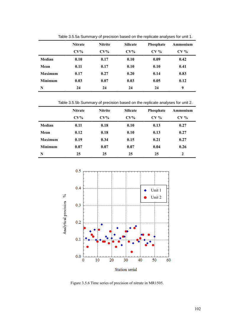
102
Table 3.5.5a Summary of precision based on the replicate analyses for unit 1.
Nitrate Nitrite Silicate Phosphate Ammonium
CV% CV% CV% CV % CV %
Median 0.10 0.17 0.10 0.09 0.42
Mean 0.11 0.17 0.10 0.10 0.41
Maximum 0.17 0.27 0.20 0.14 0.83
Minimum 0.03 0.07 0.03 0.05 0.12
N 24 24 24 24 9
Table 3.5.5b Summary of precision based on the replicate analyses for unit 2.
Nitrate Nitrite Silicate Phosphate Ammonium
CV% CV% CV% CV % CV %
Median 0.11 0.18 0.10 0.13 0.27
Mean 0.12 0.18 0.10 0.13 0.27
Maximum 0.19 0.34 0.15 0.21 0.27
Minimum 0.07 0.07 0.07 0.04 0.26
N 25 25 25 25 2
Figure 3.5.6 Time series of precision of nitrate in MR1505.
◆ Unit 1
● Unit 2

103
Figure 3.5.7 Time series of precision of phosphate in MR1505.
Figure 3.5.8 Time series of precision of silicate in MR1505.
◆ Unit 1
● Unit 2
◆ Unit 1
● Unit 2

104
(7.2) CRM lot. BV measurement during this cruise
CRM lot. BV was measured every run to monitor the comparability among runs. The results of lot.
BV during this cruise are shown as Figures 3.5.9 to 3.5.11. Error bars represent analytical precision in
figure 3.5.6 to 3.5.8.
Figure3.5.9 Time series of CRM-BV of nitrate in MR1505.
Figure 3.5.10 Time series of CRM-BV of phosphate in MR1505.

105
Figure 3.5.11 Time series of CRM-BV of silicate in MR1505.
(7.3) Carryover
We can also summarize the magnitudes of carryover throughout the cruise. These are small enough
within acceptable levels as shown in Table 3.5.8 and Figures 3.5.12 to 3.5.14. The carryover in nitrate and
silicate had a bias by equipments. It was 0.06% and 0.05%, mean value, at Unit 2. The other hand, it was
0.17% and 0.13 %, mean value, at Unit 1. We carried out the maintenance for Unit 1 by changing for new
glass coils and new transmission tube before the stn. 22. The bias was clearly solved by the maintenance.
Table 3.5.6 Summary of carry over throughout MR1505.
Nitrate Nitrite Silicate Phosphate Ammonium
CV% CV% CV% CV % CV %
Median 0.10 0.11 0.07 0.10 0.42
Mean 0.12 0.10 0.09 0.11 0.39
Maximum 0.28 0.40 0.23 0.17 0.67
Minimum 0.03 0.00 0.03 0.05 0.08
N 49 49 49 49 11

106
Figure 3.5.12 Time series of carryover of nitrate in MR1505.
Figure 3.5.13 Time series of carryover of phosphate in MR1505.
◆ Unit 1
● Unit 2
◆ Unit 1
● Unit 2 ◆ Unit 1
● Unit 2
◆ Unit 1
● Unit 2

107
Figure 3.5.14 Time series of carryover of silicate in MR1505.
(7.4) Estimation of uncertainty of phosphate, nitrate and silicate concentrations
Empirical equations, eq. (1), (2) and (3) to estimate uncertainty of measurement of phosphate, nitrate
and silicate are used based on measurements of 24 sets of CRMs during this cruise. Empirical equations,
eq. (4) and (5) to estimate uncertainty of measurement of nitrite and ammonium are used based on
duplicate measurements of the samples. These empirical equations and graphic presentation of equations
are as follows, respectively.
Phosphate Concentration Cp in μmol kg-1:
Uncertainty of measurement of phosphate (%) =
0.142 + 0.136 * (1 / Cp) +0.005 * (1 / Cp) * (1 / Cp) --- (1)
where Cp is phosphate concentration of sample.
Nitrate Concentration Cno3 in μmol kg-1:
Uncertainty of measurement of nitrate (%) =
0.08 + 1.49 * (1 / Cno3) + 0.02 * (1 / Cno3) *(1 / Cno3) --- (2)
where Cno3 is nitrate concentration of sample.
◆ Unit 1
● Unit 2 ◆ Unit 1
● Unit 2

108
Silicate Concentration Cs in μmol kg-1:
Uncertainty of measurement of silicate (%) =
0.11 + 0.96 * (1 / Cs) + 3.74 * (1 / Cs) * (1 / Cs) --- (3)
where Cs is silicate concentration of sample.
Nitrite Concentration Cno2 in μmol kg-1:
Uncertainty of measurement of nitrite (%) =
- 0.10 + 0.18 * (1 / Cno2) + 0.000022 * (1 / Cno2) * (1 / Cno2) --- (4)
where Ca is ammonium concentration of sample.
Ammonium Concentration Ca in μmol kg-1:
Uncertainty of measurement of ammonium (%) =
10.8 + 0.9 * (1 / Ca) + 0.003 * (1 / Ca) * (1 / Ca) --- (5)
where Ca is ammonium concentration of sample.
Figure 3.5.15 Estimation of uncertainty for phosphate in MR1505.

109
Figure 3.5.16 Estimation of uncertainty for nitrate in MR1505.
Figure 3.5.17 Estimation of uncertainty for silicate in MR1505.

110
Figure 3.5.18 Estimation of uncertainty for nitrite in MR1505.
Figure 3.5.19 Estimation of uncertainty for ammonium in MR1505.

111
(8) Problems / improvements occurred and solutions
(8.1) squashed air tube
We found that peak shape at 1ch became broad in the middle of run for stn. 50. And segment air into
inlet were too small. Then we found air tube to inlet was squashed by manifold cover. Because samples
concentration of broad peak shape were lower than same samples of normal peak shape, we analysed
again all samples of stn. 50. We accepted NO3 data of second run and others of first run for stn. 50.
(8.2) Phosphate channel
Phosphate channel we observe slightly higher concentration of 0.015 μmol kg-1 for lot BZ in
terms of average of 49 runs, and slightly lower concentration of 0.006 μmol kg-1 for lot BV in terms
of average of 50 runs respectively. Most likely reason of these differences we found state above is
optics/electronics malfunction of this channel of this analyzers.
(8.3) Improvement of reduction rate at nitrate measurement
Because of decrease of absorbance of maximum concentration of in-house standard solution, we
changed a kind of pumptube of sample line at 1ch from ORG/WHT to ORG/YEL. In using ORG/WHT
pumptube, absorbance of maximum concentration of In-house standard solution was nearly 0.2. after
changed, absorbance was 1.2. As flow rate of sample became more slowly, we achieved a good stable and
high reduction rate which was 99.7% (+ 0.4% - 0.7%) in terms of mean of 50 runs during this cruise.
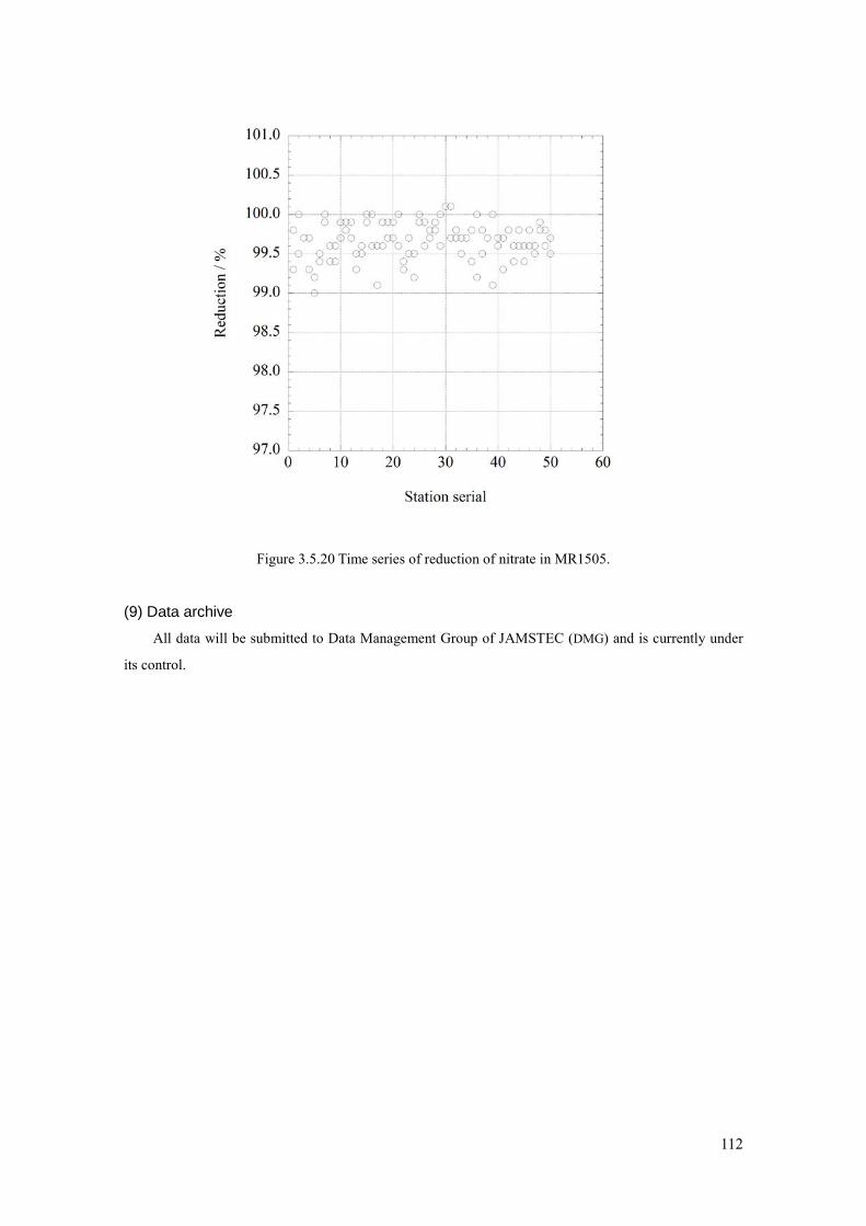
112
Figure 3.5.20 Time series of reduction of nitrate in MR1505.
(9) Data archive
All data will be submitted to Data Management Group of JAMSTEC (DMG) and is currently under
its control.

113
References Aminot, A. and Kerouel, R. 1991. Autoclaved seawater as a reference material for the determination of
nitrate and phosphate in seawater. Anal. Chim. Acta, 248: 277-283.
Aminot, A. and Kirkwood, D.S. 1995. Report on the results of the fifth ICES intercomparison exercise for
nutrients in sea water, ICES coop. Res. Rep. Ser., 213.
Aminot, A. and Kerouel, R. 1995. Reference material for nutrients in seawater: stability of nitrate, nitrite,
ammonia and phosphate in autoclaved samples. Mar. Chem., 49: 221-232.
Aoyama M., and Joyce T.M. 1996, WHP property comparisons from crossing lines in North Pacific. In
Abstracts, 1996 WOCE Pacific Workshop, Newport Beach, California.
Aoyama, M., 2006: 2003 Intercomparison Exercise for Reference Material for Nutrients in Seawater in a
Seawater Matrix, Technical Reports of the Meteorological Research Institute No.50, 91pp, Tsukuba,
Japan.
Aoyama, M., Susan B., Minhan, D., Hideshi, D., Louis, I. G., Kasai, H., Roger, K., Nurit, K., Doug, M.,
Murata, A., Nagai, N., Ogawa, H., Ota, H., Saito, H., Saito, K., Shimizu, T., Takano, H., Tsuda, A.,
Yokouchi, K., and Agnes, Y. 2007. Recent Comparability of Oceanographic Nutrients Data: Results of
a 2003 Intercomparison Exercise Using Reference Materials. Analytical Sciences, 23: 1151-1154.
Aoyama M., J. Barwell-Clarke, S. Becker, M. Blum, Braga E. S., S. C. Coverly,E. Czobik, I. Dahllof, M.
H. Dai, G. O. Donnell, C. Engelke, G. C. Gong, Gi-Hoon Hong, D. J. Hydes, M. M. Jin, H. Kasai, R.
Kerouel, Y. Kiyomono, M. Knockaert, N. Kress, K. A. Krogslund, M. Kumagai, S. Leterme, Yarong
Li, S. Masuda, T. Miyao, T. Moutin, A. Murata, N. Nagai, G.Nausch, M. K. Ngirchechol, A. Nybakk,
H. Ogawa, J. van Ooijen, H. Ota, J. M. Pan, C. Payne, O. Pierre-Duplessix, M. Pujo-Pay, T. Raabe, K.
Saito, K. Sato, C. Schmidt, M. Schuett, T. M. Shammon, J. Sun, T. Tanhua, L. White, E.M.S.
Woodward, P. Worsfold, P. Yeats, T. Yoshimura, A.Youenou, J. Z. Zhang, 2008: 2006 Intercomparison
Exercise for Reference Material for Nutrients in Seawater in a Seawater Matrix, Technical Reports of
the Meteorological Research Institute No. 58, 104pp.
Aoyama, M., Nishino, S., Nishijima, K., Matsushita, J., Takano, A., Sato, K., 2010a. Nutrients, In: R/V
Mirai Cruise Report MR10-05. JAMSTEC, Yokosuka, pp. 103-122.
Aoyama, M., Matsushita, J., Takano, A., 2010b. Nutrients, In: MR10-06 preliminary cruise report.
JAMSTEC, Yokosuka, pp. 69-83
Gouretski, V.V. and Jancke, K. 2001. Systematic errors as the cause for an apparent deep water property
variability: global analysis of the WOCE and historical hydrographic data・REVIEW ARTICLE,
Progress In Oceanography, 48: Issue 4, 337-402.
Grasshoff, K., Ehrhardt, M., Kremling K. et al. 1983. Methods of seawater anylysis. 2nd rev. Weinheim:
VerlagChemie, Germany, West.
Hydes, D.J., Aoyama, M., Aminot, A., Bakker, K., Becker, S., Coverly, S., Daniel, A., Dickson, A.G.,
Grosso, O., Kerouel, R., Ooijen, J. van, Sato, K., Tanhua, T., Woodward, E.M.S., Zhang, J.Z., 2010.
Determination of Dissolved Nutrients (N, P, Si) in Seawater with High Precision and

114
Inter-Comparability Using Gas-Segmented Continuous Flow Analysers, In: GO-SHIP Repeat
Hydrography Manual: A Collection of Expert Reports and Guidelines. IOCCP Report No. 14, ICPO
Publication Series No 134.
Joyce, T. and Corry, C. 1994. Requirements for WOCE hydrographic programmed data reporting. WHPO
Publication, 90-1, Revision 2, WOCE Report No. 67/91.
Kawano, T., Uchida, H. and Doi, T. WHP P01, P14 REVISIT DATA BOOK, (Ryoin Co., Ltd., Yokohama,
2009).
Kimura, 2000. Determination of ammonia in seawater using a vaporization membrane permeability
method. 7th auto analyzer Study Group, 39-41.
Kirkwood, D.S. 1992. Stability of solutions of nutrient salts during storage. Mar. Chem., 38 : 151-164.
Kirkwood, D.S. Aminot, A. and Perttila, M. 1991. Report on the results of the ICES fourth
intercomparison exercise for nutrients in sea water. ICES coop. Res. Rep. Ser., 174.
Mordy, C.W., Aoyama, M., Gordon, L.I., Johnson, G.C., Key, R.M., Ross, A.A., Jennings, J.C. and
Wilson. J. 2000. Deep water comparison studies of the Pacific WOCE nutrient data set. Eos
Trans-American Geophysical Union. 80 (supplement), OS43.
Murphy, J., and Riley, J.P. 1962. Analyticachim. Acta 27, 31-36.
Sato, K., Aoyama, M., Becker, S., 2010. CRM as Calibration Standard Solution to Keep Comparability
for Several Cruises in the World Ocean in 2000s. In: Aoyama, M., Dickson, A.G., Hydes, D.J., Murata,
A., Oh, J.R., Roose, P., Woodward, E.M.S., (Eds.), Comparability of nutrients in the world’s ocean.
Tsukuba, JAPAN: MOTHER TANK, pp 43-56.
Uchida, H. &Fukasawa, M. WHP P6, A10, I3/I4 REVISIT DATA BOOK Blue Earth Global Expedition
2003 1, 2, (Aiwa Printing Co., Ltd., Tokyo, 2005).

3.6 Chlorofluorocarbons and Sulfur hexafluoride
Ken’ichi Sasaki1), Hironori Sato2), Katsunori Sagishima2), and Hiroshi Hoshino2)
1) Mutsu Institute for Oceanography, Japan Agency for Marine Earth Science and Technology
2) Marine Works Japan Ltd.
3.6.1 Objectives
Chlorofluorocarbons (CFCs) and sulfur hexafluoride (SF6) are man-made stable gases. These
atmospheric gases can slightly dissolve in sea surface water by air-sea gas exchange and then are
spread into the ocean interior. So dissolved these gases could be used as chemical tracers for the ocean
circulation. We measured concentrations of three chemical species of CFCs, CFC-11 (CCl3F), CFC-12
(CCl2F2), and CFC-113 (C2Cl3F3), and SF6 in seawater on board, and made simultaneous analysis of
dissolved nitrous oxide (N2O) for a certain number of seawater samples on the trial base.
3.6.2 Apparatus
We use three measurement systems. One of them is CFCs analyzing system. Other two are
SF6/CFCs simultaneous analyzing system. Trial analysis of N2O was made on latter systems. Both
systems are based on purging and trapping gas chromatography.
Table 3-5-1 Instruments
SF6/CFCs (&N2O) simultaneous analyzing system
Gas Chromatograph: GC-14B (Shimadzu Ltd.) Detector 1: ECD-14 (Shimadzu Ltd.)
Detector 2: ECD-14 (Shimadzu Ltd.)
Analytical Column:
Pre-column 1: Silica Plot capillary column [i.d.: 0.53 mm, length: 6 m, film thickness: 6
µm]
Pre-column 2: Molesive 5A Plot capillary column [i.d.: 0.53 mm, length: 5 m, film
thickness: 15 µm]
Main column 1&2: Connected two capillary columns (Pola Bond-Q [i.d.: 0.53mm, length: 9
m, film thickness: 10µm] followed by Silica Plot [i.d.: 0.53mm, length:
18 m, film thickness: 6µm])
Purging & trapping: Developed in JAMSTEC. Cold trap columns are 30 cm length stainless
steel tubing packed the section of 5cm with 80/100 mesh Porapak Q and
followed by the section of 5cm of 100/120 mesh Carboxen 1000. Outer

116
diameters of the main and focus trap columns are 1/8” and 1/16”,
respectively.
CFCs analyzing system
Gas Chromatograph: GC-14B (Shimadzu Ltd.) Detector: ECD-14 (Shimadzu Ltd.)
Analytical Column:
Pre-column: Silica Plot capillary column [i.d.: 0.53mm, length: 6 m, film thickness:
6µm]
Main column: Connected two capillary columns (Pola Bond-Q [i.d.: 0.53mm, length: 9
m, film thickness: 10µm] followed by Silica Plot [i.d.: 0.53mm, length:
18 m, film thickness: 6µm])
Purging & trapping: Developed in JAMSTEC. Cold trap columns are 1/16” SUS tubing
packed the section of 5cm with 100/120 mesh Porapak T.
3.6.3 Procedures
3.6.3.1 Sampling
Seawater sub-samples were collected from 12 liter Niskin bottles to 450 ml of glass bottles
developed in JAMSTEC. The glass bottles were filled by CFC free gas (pure nitrogen gas) before
sampling. Two times of the bottle volume of seawater sample were overflowed. The seawater samples
were kept in water bath controlled at 7ºC. The samples were taken to determination as soon as possible
after sampling (usually within 12 hours).
In order to confirm CFC/SF6 concentrations of standard gases and their stabilities and also to check
saturation levels in sea surface water, mixing ratios in background air were periodically analyzed. Air
samples were continuously led into laboratory by air pump. The end of 10 mm OD Dekaron tubing was
put on a head of the compass deck and another end was connected onto the air pump in the laboratory.
The tubing was relayed by a T-type union which had a small stop cock. Air sample was collected from
the flowing air into a 200ml glass cylinder attached on the cock.
3.6.3.2 Analysis
SF6/CFCs (/N2O) simultaneous analyzing system
Constant volume of sample water (200 ml) is taken into a sample loop. The sample is send into
stripping chamber and dissolved SF6, CFCs and N2O are de-gassed by N2 gas purging for 8 minutes.
The gas sample is dried by magnesium perchlorate desiccant and concentrated on a main trap column
cooled down to -80 ºC. Stripping efficiencies are frequently confirmed by re-stripping of surface layer

117
samples and more than 99 % of dissolved SF6 and CFCs and ~95 % of N2O are extracted on the first
purge. Following purging & trapping, the main trap column is isolated and electrically heated to 170 ºC.
After 1 minute, the desorbed gases are sent onto focus trap cooled down to -80 ºC for 30 seconds.
Gaseous sample on the focus trap are desorbed by same manner of the main trap, and lead onto the
pre-column 1 (PC 1). Sample gases are roughly separated on the PC 1. Eluting SF6, CFCs and N2O onto
pre-column 2 (PC 2), PC1 is connected onto cleaning line and high boiling point compounds are
flushed by counter flow of pure nitrogen gas. SF6 and CFCs are rapidly eluted from PC 2 onto
main-column 1 (MC 1) and N2O is retained on PC 2. Then PC 2 is connected back-flush carrier gas line
and N2O is sent onto main-column 2 (MC 2). SF6 and CFCs are further separated on MC 1 and detected
by ECD 1. N2O sent onto MC 2 is detected by ECD 2.
CFCs analyzing system
Constant volume of sample water (50 ml) is taken into a sample loop. The sample is send into
stripping chamber and dissolved CFCs are de-gassed by N2 gas purging for 8 minutes. The gas sample
is dried by magnesium perchlorate desiccant and concentrated on a trap column cooled down to -50 ºC.
Stripping efficiencies are frequently confirmed by re-stripping of surface layer samples and more than
99.5 % of dissolved CFCs are extracted on the first purge. Following purging & trapping, the trap
column is isolated and electrically heated to 140 ºC. The desorbed gases are lead into the pre-column.
Sample gases are roughly separated in the pre-column. When CFC-113 eluted from pre-column onto
main column, the pre-column is connected onto another line and flushed by counter flow of pure
nitrogen gas. CFCs send on MC 1 are further separated and detected by ECD.
Nitrogen gases used in these systems was filtered by gas purifier column packed with Molecular
Sieve 13X (MS-13X).
Table 3-5-2 Analytical conditions
SF6/CFCs(/N2O) simultaneous analyses
Temperature
Analytical Column: 95 ºC
Detector (ECD): 300 ºC
Trap column: -80 ºC (at adsorbing) & 170 ºC (at desorbing)
Mass flow rate of nitrogen gas (99.99995%)
Carrier gas 1: 10 ml/min
Carrier gas 2: 10 ml/min
Detector make-up gas 1: 27 ml/min
Detector make-up gas 2: 27 ml/min

118
Back flush gas: 10 ml/min
Sample purge gas: 220 ml/min
CFCs analyses
Temperature
Analytical Column: 95 ºC
Detector (ECD): 240 ºC
Trap column: -50 ºC (at adsorbing) & 140 ºC (at desorbing)
Mass flow rate of nitrogen gas (99.99995%)
Carrier gas : 10 ml/min
Detector make-up gas : 27 ml/min
Back flush gas: 10 ml/min
Sample purge gas: 130 ml/min
Standard gas (Japan Fine Products co. Ltd.)
Cylinder No. Base gas CFC-11 CFC-12 CFC113 SF6 N2O remarks
ppt ppt ppt ppt ppm
CPB28497 N2 901 485 78.8 10.10 14.9 for SF6/CFC
CPB26840 N2 889 481 81.4 9.98 14.9 for SF6/CFC
CPB16993 N2 300 160 29.9 0.0 0.0 for CFC
CPB15651 N2 300 161 29.8 0.0 0.0 Reference
3.6.4 Performance
The analytical precisions are estimated from replicate sample analyses. The estimated preliminary
precisions were ± 0.005 pmol/kg (n = 143), ± 0.007 pmol/kg (n = 143), ± 0.003 pmol/kg (n = 121), and ±
0.021 fmol/kg (n = 96) for CFC-11, CFC-12, CFC-113, and SF6, respectively. Analyses of N2O had
serious problems probably caused by error of standard gas composition. Evaluating the standard gas
composition, we may report the N2O data later (but as bad data).
3.6.5 Data archive
All data will be submitted to Data Management Group of JAMSTEC (DMG) and under its control.

119
3.7. Carbon items (1) Personnel
Akihiko Murata (JAMSTEC)
Tomonori Watai (MWJ)
Makoto Takada (MWJ)
Atsushi Ono (MWJ)
Kanako Yoshida (MWJ)
(2) Objectives
Concentrations of CO2 in the atmosphere are now increasing at a rate of about 2.0 ppmv y–1
owing to human activities such as burning of fossil fuels, deforestation, and cement production. It is an
urgent task to estimate as accurately as possible the absorption capacity of the oceans against the
increased atmospheric CO2, and to clarify the mechanism of the CO2 absorption, because the magnitude
of the anticipated global warming depends on the levels of CO2 in the atmosphere, and because the ocean
currently absorbs 1/3 of the 6 Gt of carbon emitted into the atmosphere each year by human activities.
The eastern part of the Indian Ocean is one of the regions where uncertainty of uptake of
anthropogenic CO2 is large. In this cruise, therefore, we were aimed at quantifying how much
anthropogenic CO2 was absorbed in the ocean interior of the eastern part of the Indian Ocean. For the
purpose, we measured CO2-system parameters such as dissolved inorganic carbon (CT), total alkalinity
(AT) and pH along the WHP I10 in the region.
(3) Apparatus
i. CT
Measurement of CT was made with a total CO2 measuring system (called as System D, Nippon
ANS, Inc.). The system comprised of a seawater dispensing system, a CO2 extraction system and a
coulometer. In this cruise, we used a coulometer Model 3000, which was constructed by Nippon ANS.
The systems had a specification as follows:
The seawater dispensing system has an auto-sampler (6 ports), which
dispenses seawater from a 300 ml borosilicate glass bottle into a pipette of about 15
ml volume by PC control. The pipette is kept at 20 °C by a water jacket, in which
water from a water bath set at 20 °C is circulated. CO2 dissolved in a seawater
sample is extracted in a stripping chamber of the CO2 extraction system by adding
phosphoric acid (~ 10 % v/v) of about 2 ml. The stripping chamber is approx. 25 cm
long and has a fine frit at the bottom. The acid is added to the stripping chamber
from the bottom of the chamber by pressurizing an acid bottle for a given time to
push out the right amount of acid. The pressurizing is made with nitrogen gas
(99.9999 %). After the acid is transferred to the stripping chamber, a seawater

120
sample kept in a pipette is introduced to the stripping chamber by the same
method as in adding an acid. The seawater reacted with phosphoric acid is stripped
of CO2 by bubbling the nitrogen gas through a fine frit at the bottom of the
stripping chamber. The CO2 stripped in the chamber is carried by the nitrogen gas
(flow rates is 140 ml min-1) to the coulometer through a dehydrating module. The
module consists of two electric dehumidifiers (kept at ~4 °C) and a chemical
desiccant (Mg(ClO4)2). The measurement sequence such as system blank (phosphoric acid blank), 1.865 % CO2 gas in a
nitrogen base, sea water samples (6) is programmed to repeat. The measurement of 1.865 % CO2 gas is
made to monitor response of coulometer solutions purchased from UIC.
ii. AT
Measurement of AT was made based on spectrophotometry using a custom-made system (Nippon
ANS, Inc.). The system comprises of a water dispensing unit, a HCl titration unit (Hamilton No.2), and a
detection unit of a spectrophotometer (TM-UV/VIS C10082CAH, Hamamatsu Photonics, Japan) and an
optical source (Mikropack, Germany). The system was automatically controlled by a PC. The water
dispensing unit had a water-jacketed pipette and a water-jacketed glass titration cell.
A seawater of approx. 42 ml was transferred from a sample bottle (borosilicate glass bottle; 130
ml) into the water-jacketed (25 ºC) pipette by pressurizing the sample bottle (nitrogen gas), and was
introduced into the water-jacketed (25 ºC) glass titration cell. The introduced seawater was used to rinse
the titration cell. After dumping the seawater used for rinse, Milli-Q water was introduced into the
titration cell to rinse it. This is repeated twice. Next, a seawater of approx. 42 ml was weighted again by
the pipette, and was transferred into the titration cell. Then, for seawater blank, absorbances were
measured at three wavelengths (750, 616 and 444 nm). After the measurement, an acid titrant, which was
a mixture of approx. 0.05 M HCl in 0.65 M NaCl and bromocresol green (BCG), was added into the
titration cell. The volume of acid titrant solution was changed according to expected values of AT from
approx. 2.2 ml to 2.0 ml. The seawater and acid titrant were mixed for 5 minutes by a stirring tip and
bubbling by nitrogen gas in the titration cell. Then, absorbances at the three wavelengths were measured
again.
Calculation of AT was made by the following equation:
[ ] SAASATT V/)VMVH(A +−= + ,
where MA is the molarity of the acid titrant added to the seawater sample, [H+]T is the total excess
hydrogen ion concentration in the seawater, and VS, VA and VSA are the initial seawater volume, the added
acid titrant volume, and the combined seawater plus acid titrant volume, respectively. [H+]T is calculated

121
from the measured absorbances based on the following equation (Yao and Byrne, 1998):
),S001005.01log())R1299.03148.2/()00131.0Rlog(()S35(002578.02699.4]Hlog[pH TT
−−−−+−+=−= +
where S is the sample salinity, and R is the absorbance ratio calculated as:
)AA()AA(R 750444750616 −−= ,
where Ai is the absorbance at wavelength i nm.
The HCl in the acid titrant was standardized on land. The concentrations of BCG were
estimated to be approx. 2.0 × 10⁻⁶ M in the sample seawater, respectively.
iii. pH
Measurement of pH was made by a pH measuring system (Nippon ANS, Inc.). For the
detection of pH, spectrophotometry was adopted. The system comprises of a water dispensing unit and a
spectrophotometer (Bio 50 Scan, Varian). For an indicator, m-cresol purple (2 mM) was used.
Seawater is transferred from borosilicate glass bottle (300 ml) to a sample cell in the
spectrophotometer. The length and volume of the cell are 8 cm and 13 ml, respectively, and the sample
cell is kept at 25.00 ± 0.05 ºC in a thermostated compartment. First, absorbance of seawater only is
measured at three wavelengths (730, 578 and 434 nm). Then the indicator is injected and circulated for
about 4 minutes to mix the indicator and seawater sufficiently. After the pump is stopped, the absorbance
of seawater + indicator is measured at the same wavelengths. The pH is calculated based on the following
equation (Clayton and Byrne, 1993):
−
−+=
)A/A(1331.02220.200691.0A/AlogpKpH
21
212 ,
where A1 and A2 indicate absorbance at 578 and 434 nm, respectively, and pK2 is calculated as a function
of water temperature and salinity.
(4) Results
Cross sections of CT, pH, and AT along WOCE I10 line are illustrated in Figs. 3.7.1, 3.7.2 and

122
3.7.3, respectively.
Fig. 3.7.1. Distributions of CT along the I10 section.
Fig. 3.7.2. Distributions of AT along the I10 section.

123
Fig. 3.7.3. Distributions of pH along the I10 section.
References
Clayton T.D. and R.H. Byrne (1993) Spectrophotometric seawater pH measurements: total hydrogen ion
concentrtaion scale calibration of m-cresol purple and at-sea results. Deep-Sea Research 40,
2115-2129.

124
3.8 Calcium and Total alkalinity 2 Calcium
(1) Personnel
Etsuro Ono (JAMSTEC)
(2) Objectives
According to the recent IPCC report, concentrations of CO2 in the atmosphere have increased by 40%
since pre-industrial times, primarily from fossil fuel emissions and secondarily from net land use change.
The ocean has absorbed about 30% of the emitted anthropogenic carbon dioxide, causing ocean
acidification. Ocean acidification is characterized by an increase of H+ (i.e., a decrease of pH) and a
concurrent decrease of carbonate ion concentration (CO32–). The decrease of CO3
2– is unfavorable to
marine calcifying organisms, which utilize CO32-, together with Ca2+, to produce their calcium carbonate
(CaCO3) shells and skeletons. To evaluate dissolution and precipitation of calcium carbonate, we
measured directly the concentration of calcium in the sea water in the subtropical region of the eastern
part of the Indian Ocean.
(3) Apparatus
Measurement of calcium was made by a modified Dissolved Oxygen Titrator DOT-01 (Kimoto
Electronic Co. Ltd.). Bandpass filter was replaced to f0=620nm.
Added reagents are as follows.
NH3/NH4buffer: 0.4 mol/l NH4Cl/ 0.4 mol/l NH3 buffer
Masking agent: 0.05 mol/l 2,2’,2”-nitrotriethanol solution
Zincon solution:
0.004 mol/l Zincon, 0.0925g Zincon was dissolved 0.8 ml 1M NaOH and was diluted to 50 ml
Zn/EGTA solution: 0.004 mol/l ZnSO4/ 0.004 mol/l EGTA
EGTA titrant: 0.02 mol/l EGTA
The system comprises of a light source, photodiode detectors, auto-burette and control unit. Seawater of
accurate 10ml was transferred from a sample bottle (60ml HDPE bottle) into 100 ml tall beaker by
volumetric pipet. A magnetic stirrer bar was added into beaker. 1ml NH3/NH4buffer, 1ml masking agent,
1ml Zincon solution, 1ml Zn/EGTA solution and about 60ml H2O were added into the beaker. The
seawater samples were titrated by the EGTA titrant. The EGTA titrant was calibrated by 1000mg/l Ca
standard solution (produced by Wako Pure Chemical Industries, Ltd.).
(4) Performances
The system worked well no troubles. The repeatability was estimated to be 0.0088±0.0080 (n=17 pairs)
mmol kg-1.

125
Fig.3.8.1 Vertical profiles of calcium.

126
Total alkalinity 2 (1) Personnel
Etsuro Ono (JAMSTEC)
(2) Objectives
Same as in “Carbon Items”
(3)Apparatus
Measurement of AT was made based on potentiometry with Total Alkalinity Titrator ATT-05 (Kimoto
Electronic Co. Ltd.). The system comprises of an auto-burette, combination electrode (pHC2001-8
S/N:13242-F17, S/N:13282-F11, Radiometer analytical) and control unit.
The in-house acid solution (approx.0.1 M HCl in 0.6 M NaCl ) was prepared as a titrant in advance
of cruise.
(4)Analysis
All measurements were carried out with open cell method.
Open cell method
Seawater of accurate 50ml was transferred from a sample bottle (glass bottle) into 100 ml tall beaker
by volumetric pipet. A magnetic stirrer bar was added into beaker. The combination electrode and
temperature sensor were immersed in sample. The seawater samples were titrated by the acid titrant.
The acid titrant was calibrated by measuring Dickson’s CRM (Batch 149). First, the acid titrant was
added until pH of sample under 3.8 and stirred for 300 seconds. Second, the acid titrant was added
by 20 µl at intervals of 15 seconds until reaching pH of 2.8. Values of AT were computed with a
program incorporated in the equipment.
The electrode of S/N:13242-17, at first, was used at station 06, 12, 16 and 24. However,
S/N:13242-17 was replaced with S/N:13282-F11 after the measurements at station 24, because
S/N:13242-17 showed such slow a response that some measured values were not computed accurate.
The measurements worked well with S/N:13282-F11 at station 28, 33, 36, 45 and 51.

127
3.9. Dissolved organic carbon and total dissolved nitrogen (1) Personnel
Masahito Shigemitsu (JAMSTEC): Principal investigator
Chisato Yoshikawa (JAMSTEC)
Masahide Wakita (JAMSTEC)
Akihiko Murata (JAMSTEC)
(2) Objectives
Dissolved organic carbon (DOC) and total dissolved nitrogen (TDN) are considered to be important
reservoirs of carbon and nitrogen in the ocean. They can also be substrates for heterotrophic microbial
communities and TDN can serve as a source of nitrogen to autotrophs in nitrogen-deficient regions.
In this cruise, we aimed to gain insights into the amount of DOC and TDN transported via the
Indonesian throughflow from the Pacific to the Indian ocean, and interactions between dissolved organic
materials like DOC and TDN and heterotrophic micro-organisms in the Indian Ocean.
(3) Material and methods
Seawater samples were obtained from Niskin bottles on a CTD-rosette system. Each sample taken in
the upper 500 m was filtered using a pre-combusted (450℃ for 4 hours) Whatman 47-mm GF/F filter.
The filtration was carried out by connecting a spigot of the Niskin bottle through silicone tube to an
inline plastic filter holder. Filtrates were collected in acid-washed 60 mL High Density Polyethylene
(HDPE) bottles in duplicates or triplicates, and were immediately stored frozen until analysis. Other
samples taken below 500 m were unfiltered and stored in the same way.
In the analysis after the cruise, the frozen samples are thawed at room temperature, and acidified to
pH < 2 with hydrochloric acid followed by being bubbled to remove dissolved inorganic carbon from
the samples. Concentrations of DOC and TDN are, then, measured by using a total organic carbon
analyzer equipped with a chemiluminescence detector unit (Shimadzu, Japan).
(4) Data archives
The data of DOC and TDN obtained in this cruise will be submitted to the Data Management Group
of JAMSTEC, and will be open to the public via “Data Research System for Whole Cruise Information in
JAMSTEC (DARWIN)” in JAMSTEC web site.

128
3.10 Chlorophyll a (1) Personnel
Kosei Sasaoka (JAMSTEC)
Keitaro Matsumoto (MWJ)
Misato Kuwahara (MWJ)
Masahiro Orui (MWJ)
Haruka Tamada (MWJ)
(2) Objectives
Chlorophyll a is one of the most convenient indicators of phytoplankton stock, and has been used
extensively for the estimation of phytoplankton abundance in various aquatic environments. In this study,
we investigated horizontal and vertical distribution of phytoplankton along the I10 section in the Eastern
Indian Ocean. The chlorophyll a data is also utilized for calibration of fluorometers, which were installed
in the surface water monitoring and CTD profiler system.
(3) Instrument and Method
Seawater samples were collected in 250 ml brown Nalgene bottles without head-space. The whole
samples were gently filtrated by low vacuum pressure (< 0.02 MPa) through Whatman GF/F filter
(diameter = 25 mm) in the dark room. Whole volume of each sampling bottle was precisely measured in
advance. After filtration, phytoplankton pigments were immediately extracted in 7 ml of
N,N-dimethylformamide (DMF), and samples were stored at -20°C under the dark condition to extract
chlorophyll a more than 24 hours. Chlorophyll a concentrations were measured by the Turner fluorometer
(10-AU-005, TURNER DESIGNS), which was previously calibrated against a pure chlorophyll a
(Sigma-Aldrich Co., LLC) (Fig. 3.10-1). To estimate the chlorophyll a concentrations, we applied to the
fluorometric “Non-acidification method” (Welschmeyer, 1994).
(4) Results
Cross section of chlorophyll a concentrations along the I10 line during the cruise is shown in Fig.
3.10-2. To estimate the measurement precision, 48-pairs of replicate samples were obtained from
hydrographic casts. All pairs of the replicate samples were collected in 250 ml bottles. Standard deviation
calculated from 48-pairs of the replicate samples was 0.078 μg/L, although absolute difference values
between 45-pairs of the replicate samples were smaller than 0.01 μg/L.
(5) Reference
Welschmeyer, N. A. (1994): Fluorometric analysis of chlorophyll a in the presence of chlorophyll b and
pheopigments. Limnor. Oceanogr., 39, 1985-1992.

129
Figure 3.10-1 Relationships between pure chlorophyll a concentrations and fluorescence light
intensity.
Figure 3.10-2 Cross section of chlorophyll a concentrations along the I10-line obtained from
hydrographic casts.

130
3.11 Absorption coefficients of particulate matter and colored dissolved organic matter (CDOM) (1) Personnel
Kosei Sasaoka (JAMSTEC)
(2) Objectives Absorption coefficients of particulate matter (phytoplankton and non-phytoplankton particles, defined
as ‘detritus’) and colored dissolved organic matter (CDOM) play an important role in determining the optical properties of seawater. In particular, light absorption by phytoplankton is a fundamental process of photosynthesis, and their chlorophyll a (Chl-a) specific coefficient, a*ph, can be essential factors for bio-optical models to estimate primary productivities. Absorption coefficients of CDOM are also important parameters to validate and develop the bio-optical algorithms for ocean color sensors, because the absorbance spectrum of CDOM overlaps that of Chl-a. The global colored detrital and dissolved materials (CDOM) distribution appears regulated by a coupling of biological, photochemical, and physical oceanographic processes all acting on a local scale, and greater than 50% of blue light absorption is controlled by CDOM (Siegel et al., 2002). Additionally, some investigators have reported that CDOM emerges as a unique tracer for diagnosing changes in biogeochemistry and the overturning circulation, similar to dissolved oxygen (e.g., Nelson et al., 2010). The objectives of this study are to understand the North-South variability of light absorption by phytoplankton and CDOM along the I10 section in the Indian Ocean. (3) Methods
Seawater samples for absorption coefficient of total particulate matter (ap(λ)) were performed using Niskin bottles and a bucket above 100m depth along the I10 section (Fig. 3.11-1, Table 3.11-1). Samples were collected in 3000ml dark bottles and filtered (500 - 3000 ml) through 25-mm What-man GF/F glass-fiber filters under a gentle vacuum (< 0.013 MPa) on board in the dark room. After filtration, the optical density of total particulate matter on filter (ODfp(λ)) between 350 and 750 nm at a rate of 1.0 nm was immediately measured by an UV-VIS recording spectrophotometer (UV-2400, Shimadzu Co.), and absorption coefficient was determined from the OD according to the quantitative filter technique (QFT) (Mitchell, 1990). A blank filter with filtered seawater was used as reference. All spectra were normalized to 0.0 at 750nm to minimize difference between sample and reference filter. To determine the optical density of non-pigment detrital particles (ODfd(λ)), the filters were then soaked in methanol for a few hours and rinsed with filtered seawater to extract and remove the pigments (Kishino et al., 1985), and its absorption coefficient was measured again by UV-2400. These measured optical densities on filters (ODfp(λ) and ODfd(λ)) were converted to optical densities in suspensions (ODsp(λ) and ODsd(λ)) using the pathlength amplification factor of Cleveland and Weidemann (1993) as follows:
ODsp(λ) = 0.378 ODfp(λ) + 0.523 ODfp(λ)2 and
ODsd(λ) = 0.378 ODfd(λ) + 0.523 ODfd(λ)2. The absorption coefficient of total particles (ap(λ) (m-1)) and non-pigment detrital particles (ad(λ) (m-1)) are computed from the corrected optical densities (ODs(λ)):
131
ap(λ) = 2.303 × ODsp(λ) / L (L = V / S), and ad(λ) = 2.303 × ODsd(λ) / L (L = V / S),
Where S is the clearance area of the filter (m2) and V is the volume filtered (m3). Absorption coefficient of phytoplankton (aph(λ)) was obtained by subtracting ad(λ) from ap(λ) as follows:
aph(λ) = ap(λ) − ad(λ).
Finally, we calculated chl-a normalized specific absorption spectra (a*ph) to divide aph by chl-a concentrations obtained from same hydrographic casts.
Seawater samples for absorption coefficient of CDOM (ay(λ)) were collected in 250ml bottles using Niskin bottles and a bucket from surface to bottom (Fig. 3.11-1, Table 3.11-1). CDOM samples were filtered using 0.2 μm Nuclepore polycarbonate filters on board. Optical densities of the CDOM (ODy(λ)) in this filtered seawater were recorded against UV-2400 in the range from 300 to 800 nm using 10-cm pathlength glass cells. Milli-Q water was used as a base line. A blank (Milli-Q water versus Milli-Q water) was subtracted from each wavelength of the spectrum. The absorption coefficient of CDOM (ay(λ) (m-1)) was calculated from measured optical densities (ODy(λ)) as follows: ay(λ) = 2.303 × ODy(λ) / L (L is the cuvette path-length (m)).
(4) Preliminary results Some examples of chl-a normalized specific absorption spectra (a*ph) were shown in Fig.3.11-2. Cross
section of CDOM (as absorption coefficient at 325 nm, unit = m-1) along the I10 section were shown in Fig. 3.11-3. (5) References Cleveland, J.S. and Weidemann, A.D., 1993, Quantifying absorption by aquatic particles: a multiple
scattering correction for glass fiber filters, Limnology and Oceanography, 38, 1321-1327.
Kishino, M., Takahashi, M., Okami, N. and Ichimura, S., 1985, Estimation of the spectral absorption coefficients of phytoplankton in the sea, Bulletin of Marine Science, 37, 634-642.
Mitchell, B.G., 1990, Algorithms for determining the absorption coefficient of aquatic particulates using the quantitative filter technique (QFT), Ocean Optics X, SPIE 1302, 137-148.
Nelson, N. B., D. A. Siegel, C. A. Carlson, and C. M. Swan, 2010, Tracing global biogeochemical cycles and meridional overturning circulation using chromophoric dissolved organic matter, Geophys. Res. Lett., 37, L03610, doi:10.1029/2009GL042325.
Siegel, D.A., Maritorena, S., Nelson, N.B., Hansell, D.A., Lorenzi-Kayser, M., 2002, Global distribution and dynamics of colored dissolved and detrital organic materials. J. Geophys. Res., 107, C12, 3228, doi:10.1029/2001JC000965.

132
Fig. 3.11-1 Location of sampling stations for absorption coefficients of phytoplankton and CDOM
along the I10 section in the Indian Ocean during MR15-05.
Table 3.11-1 List of sampling stations for absorption coefficients of phytoplankton (Ap) and CDOM during MR15-05.

133
Fig.3.11-2 Examples of chlorophyll-specific phytoplankton absorption coefficient spectra (a*ph(λ))
at 400-750 nm, (a) Stn.01, (b) Stn.06, (c) Stn.28, (d) Stn.52. All spectra were normalized to 0.0 at
750nm.
Fig.3.11-3 Contours showing distribution of CDOM (as absorption coefficient at 325 nm, unit = m-1)
along the I10 section during MR15-05.
400 450 500 550 600 650 700 7500.00
0.02
0.04
0.06
0.08
0.10
0m 71m 50m 10m
Wavelength (nm)
(a) Stn.01Specific
abso
rption a
*
ph(λ
) (m
2 m
g-1)
400 450 500 550 600 650 700 7500.00
0.02
0.04
0.06
0.08
0.10
0.12
0m 100m 50m 10m
Wavelength (nm)
(c) Stn.28
Specific
abso
rption a
*
ph(λ
) (m
2 m
g-1)
[m-1]
400 450 500 550 600 650 700 7500.00
0.02
0.04
0.06
0.08
0.10
0.12
0m 100m 50m 10m
Wavelength (nm)
(b) Stn.06
Specific
abso
rption a
*
ph(λ
) (m
2 m
g-1)
400 450 500 550 600 650 700 7500.00
0.02
0.04
0.06
0.08
0.10
0.12
0m Chlmax(62m) 100m 50m 10m
Wavelength (nm)
(d) Stn.52
Specific
abso
rption a
*
ph(λ
) (m
2 m
g-1)

134
3.12 Bio-sampling 3.12.1 Vertical profiles of microbial abundance, activity and diversity in the eastern Indian Ocean
(1) Personnel
Taichi Yokokawa (JAMSTEC)
Michinari Sunamura (University of Tokyo)
Takuro Nunoura (JAMSTEC)
Hirai Miho (JAMSTEC)
Chisato Yoshikawa (JAMSTEC)
Kanta Chida (Rakuno Gakuen University)
(2) Introduction
Prokaryotes (Bacteria and Archaea) play a major role in marine biogeochemical fluxes.
Biogeochemical transformation rates and functional diversity of microbes are representative major topics
in marine microbial ecology. However, the link between prokaryotes properties and biogeochemistry in
the meso- and bathypelagic layers has not been explained systematically despite of the recent studies that
highlight the role of microbes in the cycling of organic matter. (Herndl and Reinthaler 2013; Yokokawa et
al. 2013). Moreover, microbial diversity and biogeography in bathypelagic and abyssal ocean and its
relationship with upper layers and deep-water circulation have also not been well studied (Nagata et al.
2010).
The objectives of this study, which analyze the water columns from sea surface to just above
the bottom of the eastern Indian Ocean, were 1) to determine the abundance of microbes; 2) to study the
heterotrophic production and chemo-autotrophic production of prokaryotes; 3) to assess the community
composition of prokaryotes; 4) to know microbial diversity through water columns along the latitudinal
transect.
(3) Methods
Microbial abundance
Samples for microbial abundances (prokaryotes, eukaryotes and viruses) were collected in
every routine cast and depth, and the three BIO casts. Samples were fixed with glutaraldehyde (final
concentration 1%) or mixed with Glycerol-EDTA, and frozen at -80°C. The abundance of microbes and
viruses will be measured by a flow cytometry in both University of Tokyo (Sunamura) and JAMSTEC
(Nunoura) after nucleic acid staining with SYBR-Green I.
Prokaryotic activity measurements 3H-leucine incorporation rate was determined as a proxy for heterotrophic or mixotrophic
prokaryotic production. Triplicate subsamples (1.5 mL) dispensed into screw-capped centrifuge tubes
amended with 10 nmol L-1 (final concentration) of [3H]-leucine (NET1166, PerkinElmer) and incubated at

135
in situ temperature (± 2°C) in the dark. One trichloroacetic acid (TCA) killed blank was prepared for each
sample. Incubation periods were 1 hour and 24 hours for the upper (0 – 250 m) and deeper (300 – bottom)
water layers, respectively. After the incubation, proteins were TCA (final conc. 5%) extracted twice by
centrifugation (15000 rpm, 10 min, Kubota 3615-sigma), followed by the extraction with ice-cold 80%
ethanol.
The relative contribution of Archaea and Bacteria to total prokaryotic leucine incorporation was
determined using antibiotics and an inhibitor; erythromycin (Sigma-Aldrich, final conc. 10 μg mL-1) for
bacteria, diphtheria toxin (Sigma-Aldrich, final conc. 10 μg mL-1) and N1-Guanyl-1,7-Diaminoheptane
(GC7, BIOSEARCH TECHNOLOGIES, final conc. 0.2 mM) for archaea, and (2-(4-carboxyphenyl)-4,
4,5,5-tetramethylimidazoline-1-oxyl-3-oxide) (carboxy- PTIO; Dojindo Molecular Technology, INC. final
conc. 100 μM) for inhibiting ammonia-oxidizing archaea (AOA).
In the laboratory the samples will be radioassayed with a liquid scintillation counter using
Ultima-GOLD (Packard) as scintillation cocktail. Quenching is corrected by external standard channel
ratio. The disintegrations per minute (DPM) of the TCA-killed blank is subtracted from the average DPM
of the samples, and the resulting DPM is converted into leucine incorporation rates.
DIC fixation was measured via the incorporation of 50 μCi of [14C]-bicarbonate (NEC086H,
PerkinElmer) in 20 ml seawater samples. Triplicate samples and formaldehyde-fixed blanks were
incubated in the dark at in situ temperature (± 4°C) for 72 h. Incubations were terminated by adding
formaldehyde (1% final concentration) to the samples.
The relative contribution of Archaea, Bacteria and AOA to total prokaryotic DIC fixation was
determined using erythromycin (Sigma-Aldrich, final conc. 10 μg mL-1), GC7 (BIOSEARCH
TECHNOLOGIES, final conc. 0.2 mM) and PTIO (Dojindo Molecular Technology, INC. final conc. 100
μM) as bacterial, archaeal and AOA inhibitors of protein synthesis, respectively, and compared with the
DIC fixation in the control sample.
In the laboratory, the samples will be filtered onto 0.2-µm polycarbonate filters. Subsequently,
the filters are fumed with concentrated HCl for 12 h. The samples will be radioassayed with a liquid
scintillation counter using Filter-count (PerkinElmer) as scintillation cocktail. Quenching is corrected by
external standard channel ratio. The disintegrations per minute (DPM) of the formaldehyde-killed blank is
subtracted from the average DPM of the samples, and the resulting DPM is converted into bicarbonate
incorporation rates.
Samples for leucin incorporation activity measurements were taken at stations 1, 6, 10, 14, 18,
22, 26, 31, 37 in the routine casts, and those for inorganic carbon fixation rates assessed at stations 10,
22, 37 in the routine casts.
Microbial diversity
Microbial cells in water samples were filtrated on cellulose acetate filter (0.2µm) and stored at
-80˚C. Environmental DNA or RNA will be extracted from the filtrated cells and used for 16S/18S rRNA
136
gene tag sequencing using MiSeq, quantitative PCR for genes for 16S rRNA, and/or metatranscriptomics.
Moreover, selected water samples were mixed with glycerol-EDTA and stored at -80˚C for single cell
genomic analyses. Samples for microbial diversity were taken at stations 1, 6, 10, 14, 18, 22, 26, 31, and
37 in the routine casts.
References
Herndl GJ, Reinthaler T (2013) Microbial control of the dark end of the biological pump. Nature
geoscience, 6:718-724
Yokokawa T, Yang Y, Motegi C, Nagata T (2013) Large-scale geographical variation in prokaryotic
abundance and production in meso- and bathypelagic zones of the central Pacific and Southern Ocean.
Limnology and Oceanography, 58:61-73
Nagata T, Tamburini C, Aristegui J, Baltar F, Bochdansky AB, Fonda-Umani S, Fukuda H, Gogou A,
Hansell DA, Hansman RL, Herndl GJ, Panagiotopulos C, Reinthaler T, Sohrin R, Verdugo P, Yamada
N, Yamashita Y, Yokokawa T, Bartlett DH (2010) Emerging concepts on microbial processes in the
bathypelagic ocean – ecology, biogeochemistry, and genomics. Deep-Sea Research II 57:1519-1536

137
3.12.2 Geochemistry and Microbiology: Nitrogen and carbon cycles in the eastern Indian Ocean
(1) Personnel
Akiko Makabe (JAMSTEC)
Chisato Yoshikawa (JAMSTEC)
Kanta Chida (Rakuno Gakuen University)
Keisuke Koba (Tokyo University of Agriculture and Technology)
Miho Hirai (JAMSTEC)
Osamu Yoshida (Rakuno Gakuen University)
Shotoku Kotajima (Tokyo University of Agriculture and Technology)
Taichi Yokokawa (JAMSTEC)
Takuro Nunoura (JAMSTEC)
(2) Introduction
Knowledge about oceanic nitrogen and carbon cycles has been dramatically changed in this
decade. In nitrogen cycle, major ammonia oxidizers were believed to be a few lineages of Proteobacteria,
but it has been revealed that archaeal ammonia oxidizers (AOA) shared more than 10% of microbial
population in dark ocean, and nitrous oxide production is necessary for the growth of AOA. In addition,
significant contribution of heterotrophic nitrogen fixation and anaerobic ammonia oxidizers are also been
found in the oceanic nitrogen cycle. On the other hand, in carbon cycle, microbial life in dark ocean
below mesopelagic water (corresponding to 200-1000 m depth range) is thought to be primarily supported
by sinking organic carbons from surface waters. However, it has been recently revealed that the deep-sea
biogeochemical cycles are more complex than previously expected, and the dark carbon fixation coupled
with nitrification and sulfur- and hydrogen-oxidations is also recognized as another significant organic
carbon source in dark ocean (Francis et al. 2007; Alonso-Sáez et al. 2010; Swan et al. 2011;
Anantharaman et al. 2013; Herndl and Reinthalar 2013).
Nitrogen cycle
The marine nitrogen cycle in surface waters is known to control biological activity in the
ocean, because inorganic forms of nitrogen such as nitrate are indispensable nutrients for phytoplankton.
Following the primary production, organic nitrogen compounds are metabolized into ammonium and low
molecular organic nitrogen compounds that are substrates for nitrification and/or nitrogen source of
microbes. Among the components of marine nitrogen cycle, Nitrous Oxide (N2O) is recognized as
significant anthropogenic greenhouse gas and a stratospheric ozone destroyer. The estimation of global
N2O flux from ocean to the atmosphere is 3.8 TgNyr-1 and the estimation varies greatly, from 1.8 to 5.8
TgNyr-1 (IPCC, 2013). This is because previous models had estimated N2O concentration from oxygen
concentration indirectly. In fact, marine N2O production processes are very complicated; hydroxylamine
oxidation during nitrification, nitrite reduction during nitrifier denitrification and nitrite reduction during

138
denitrification produce N2O and N2O deduction during denitrification consumes N2O (Dore et al. 1998;
Knowles et al. 1981; Rysgaard et al. 1993; Svensson 1998; Ueda et al. 1993). In addition, currently,
previously unknown systems in nitrification in AOA have been reported. One is the N2O production with
unknown pathway using NO as one of the substrate (Santoro et al. 2011; Stieglmeier et al. 2014), and the
other is ammonia oxidation via urea degradation in AOA has also been reported (Alonso-Sáez et al. 2012).
Therefore marine N2O production processes are poorly understood quantitatively. N2O isotopomers
(oxygen isotope ratio (δ18O), difference in abundance of 14N15N16O and 15N14N16O (SP), and average
nitrogen isotope ratio (δ15N)) are useful tracers to distinguish these processes and had revealed N2O
production processes in various ocean environments (e.g., Yoshida and Toyoda, 2000), but we need to
improve the model with novel findings in the marine nitrogen cycle.
To reduce the uncertainties in global N2O budget a marine N2O model constrained by isotope
dataset was developed and applied to the western North Pacific (Yoshikawa et al., in press). In this study
we conducted water sampling for isotope analysis of N2O and related substances (NO3-, phytoplankton
and Chlorophyll-a) and some key reaction rates (nitrification rates) at three MBC shallow stations (above
500 m). By using the results of isotope analysis we will apply the model to the Indian Ocean and estimate
the sea to air N2O flux there. Moreover, we examine both inorganic and organic carbon uptake activity
associated with AOA during and after the cruise, and identify genetic markers for each process of nitrogen
cycle by molecular biology techniques.
Methane in ocean
The atmospheric concentrations of the greenhouse gases methane (CH4) have increased since
1750 due to human activity. In 2011 the concentrations of CH4 was 1803 ppb exceeded the pre-industrial
levels by about 150% (IPCC 2013). In order to understand the current global CH4 cycle, it is necessary to
quantify its sources and sinks. At present, there remain large uncertainties in the estimated CH4 fluxes
from sources to sinks. The ocean’s source strength for atmospheric CH4 should be examined in more
detail, even though it might be a relatively minor source, previously reported to be 0.005 to 3% of the
total input to the atmosphere (Cicerone and Oremland 1988; Bange et al. 1994; Lelieveld et al. 1998).
To estimate an accurate amount of the CH4 exchange from the ocean to the atmosphere, it is
necessary to explore widely and vertically. Distribution of dissolved CH4 in surface waters from diverse
locations in the world ocean is often reported as a characteristic subsurface maximum representing a
supersaturation of several folds (Yoshida et al. 2004; 2011). Although the origin of the subsurface CH4
maximum is not clear, some suggestions include advection and/or diffusion from local anoxic
environment nearby sources in shelf sediments, and in situ production by methanogenic bacteria,
presumably in association with suspended particulate materials (Karl and Tilbrook 1994; Katz et al. 1999).
These bacteria are thought to probable live in the anaerobic microenvironments supplied by organic
particles or guts of zooplankton (Alldredge and Cohen 1987).
So, this study investigates in detail profile of CH4 concentration in the water column in the

139
Eastern Indian Ocean to clarify CH4 dynamics and estimate the flux of CH4 to the atmosphere.
(3) Materials and methods
Seawater samples are taken by CTD-CAROUSEL system attached Niskin samplers of 12 L at
15 layers above 500 m and surface layer taken by plastic bucket at hydrographic stations as shown in
Table 1.
Table 1. Parameters and hydrographic station names for this study.
Parameters Hydrographic stations
1. δ15N and δ18O of NO3- 1, 6, 10, 14, 18, 22, 26, 31, 37
2. δ15N of Chlorophyll a
3. δ15N of Phytoplankton
10, 22, 37
10, 22, 37
4. δ15N, SP and δ18O of dissolved N2O 1, 6, 10, 14, 18, 22, 26, 31, 37
5. Nitrification rate 1, 6, 10, 18, 22, 26, 31, 37
6. Dissolved CH4 and N2O concentration 1, 4, 6, 8, 10, 14, 18, 22, 26, 28, 31, 35, 37
7. F430 10, 22, 37
8. δ13C of CH4 1, 6, 10, 14, 18, 22, 26, 31, 37
Isotopic analyses for N2O, NO3-, chlorophyll a and phytoplankton, and concentration analyses for N2O
and CH4
Sample for N2O isotopomer analysis was transferred to two of 100 ml glass vials. After an
approximately two-fold volume overflow, 200μL of saturated HgCl2 solution were added. The vials were
sealed with butyl rubbers and aluminum caps and stored in dark at 4°C until analysis. The δ15N, δ18O and
SP values and concentrations of N2O in seawater will be determined by slightly modified version of
GC-IRMS (PreCon/HP6890 GC/ MAT 252) at TIT described in detail in Yamagishi et al. (2007).
Sample for nitrate isotope analysis was collected into a 50 ml syringe equipped with a DISMIC®
filter (pore size: 0.45 μm) and filtered immediately after sampling. These samples were removed nitrite
with sulfamic acid using the method of Granger and Sigman (2009) and preserved at -23°C until chemical
analysis. The δ15N and δ18O values of NO3- will be measured using the “bacterial” method of Sigman et
al., (2001) in which N2O converted from nitrate is analyzed using GasBench/ PreCon/IRMS.
Sample for chlorophyll isotope analysis was collected into a 20L light-blocking polypropylene
tanks. The samples were filtered under reduced pressure and collected on two-three pre-combusted
Whatman GF-75 filters. The filters were double up and wrapped in aluminum foil and stored at -23°C
until analysis. Chlorophyll pigments will be extracted and split into each pigments by HPLS. The δ15N
values of Chlorophyll pigments will be measured by using EA-IRMS at JAMSTEC.
Sample for phytoplankton isotope analysis was collected into a 20L light-blocking
polypropylene tanks. The samples were condensed using an ultrafiltration system and sorted for

140
phytoplankton samples using a cell sorter. The phytoplankton samples were filtered under reduced
pressure and collected on pre-combusted Whatman GF-75 filters. The filters were stored at -23°C until
analysis. The δ15N values of phytoplankton will be measured by using EA-IRMS at JAMSTEC.
Sample for N2O and CH4 concentration analyses were carefully subsampled into 30 mL glass
vials to avoid air contamination for analyses of N2O and CH4 concentration. The seawater samples were
poisoned by 20 μL (30 mL vials) of mercuric chloride solution (Tilbrook and Karl 1995; Watanabe et al.
1995), and were closed with rubber-aluminum and plastic caps. These were stored in a dark and cool
place until we got to land, where we conducted gas chromatographic analyses of N2O and CH4
concentration at the laboratory.
Nitrification activity measurements
Water samples for nitrification activity analysis were transferred into 100 mL glass vials
without headspace. Combination of 15N enriched substrates (ammonium, urea, and glutamine (amide
group)) and inhibitors (carboxy-PTIO, allylthiourea, and GC7) were added to each vial. The final
concentration of 15N enriched substrates was 50 nM. The glass vials were incubated in dark for 12 hours
or 3 days at in situ temperature. After incubation, the samples for nitrate analysis were filtered with a
DISMIC® filter (pore size: 0.45 μm) and frozen until analysis. The samples for N2O analysis were added
by 0.2 mL of saturated HgCl2 solution and stored at 4 ºC until analysis. The 15N enrichment of nitrates
will be measured by GC-IRMS after conversion to N2O using the “bacterial” method of Sigman et al.
(2001). The 15N enrichment of N2O will be measured by GC-IRMS described in detail in Yamagishi et al.
(2007).
Nitrous oxide and methane concentration measurements
The measurement system consists of a purge and trap unit, a desiccant unit, rotary valves, gas
chromatograph equipped with a electron capture detector for concentration of N2O and a flame ionization
detector for concentration of CH4, and data acquisition units. The entire volume of seawater in each glass
vial was processed all at once to avoid contamination and loss of N2O and CH4. Precision obtained from
replicate determinations of N2O and CH4 concentration was estimated to be better than 5% for the usual
concentration in seawater.
Isotopic analysis of methane
Water samples for δ13C-CH4 analysis were transferred to 100 mL glass vials from the Niskin
sampler without headspace. After the vials were sealed with butyl rubber and aluminum caps, 200 μL of
saturated HgCl2 solution was added. The water samples were stored until analysis on land. The δ13C value
of Methane will be measured using isotope ratio mass spectrometry using a method of Tsunogai et al.
(1998 and 2000).

141
Biomarker of methanogens
Water samples for F430 analysis (5 or 10 L) were filtered (0.01 MPa) with a Whatman GF-75
filter (47 mm in diameter). The filter samples were wrapped with aluminum foil and stored at −20°C prior
to analysis on land. Extraction and analysis of F430 will be conducted at JAMSTEC using a method of
Kaneko et al. (2014).
Prokaryotic uptakes of organic and inorganic carbon measurements
See “Prokaryotic activity measurements” in the chapter “Vertical profiles of aquatic microbial
abundance, activity and diversity in the eastern Indian Ocean”.
Genetic markers of geochemical processes
Microbial cells in water samples were filtrated on cellulose acetate filter (0.2µm) and stored at
-80˚C. Environmental DNA or RNA will be extracted from the filtrated cells and used for molecular
analyses (e.g. clone analysis and quantitative PCR) to investigate the microbial components related to
nitrification, nitrogen fixation and methanogenesis.
(4) Expected results
Nitrogen cycle and microbial carbon uptake associated with nitrogen cycle
In the surface layer, N2O concentration of water affects the sea-air flux directly (Dore et al.
1998). However the pathway of N2O production in surface layer is still unresolved. In the surface layer,
N2O is predominantly produced by nitrification, but also by nitrifer-denitrification and denitrification if
oxygen concentration is low in the water mass or particles (Maribeb and Laura, 2004). The observed
concentrations and isotopomer ratios of N2O together with those values of substrates for N2O (NO3-,
phytoplankton and Chlorophyll-a) will reveal the pathway of N2O production in the surface layer and will
improve the marine N2O isotopomer model. Moreover, the horizontal isotope dataset will help to apply
the model to the Indian Ocean.
Methane
Subsurface maximum concentrations of CH4 (>3 nmol kg-1) were expected to be observed in
the Indian Ocean. A commonly-encountered distribution in the upper ocean with a CH4 peak within the
pycnocline (e.g., Ward et al. 1987; Owens et al. 1991; Watanabe et al. 1995; Yoshida et al. 2011). Karl
and Tilbrook (1994) suggested the suboxic conditions would further aid the development of
microenvironments within particles in which CH4 could be produced. The organic particles are
accumulated in the pycnocline, and CH4 is produced in the micro reducing environment by methanogenic
bacteria. Moreover, in situ microbial CH4 production in the guts of zooplankton can be expected (e.g.,
Owens et al. 1991; de Angelis and Lee 1994; Oudot et al. 2002; Sasakawa et al. 2008). Watanabe et al.
142
(1995) pointed out that the diffusive flux of CH4 from subsurface maxima to air-sea interface is sufficient
to account for its emission flux to the atmosphere. In the mixed layer above its boundary, the CH4 is
formed and discharged to the atmosphere in part, in the below its boundary, CH4 diffused to the bottom
vertically. By using concentration and isotopic composition of CH4 and hydrographic parameters for
vertical water samples, it is possible to clarify its dynamics such as production and/or consumption in the
water column.
A depth profile of F430 concentration in water column will provide information about
quantitative distribution of methanogens. The δ13C value of methane reflects carbon source and
methaogenic pathway (Whiticar, 1999). If the profile correlate with other chemical profiles including
concentrations of methane, chlorophyll and dissolved oxygen, it can be a strong evidence of that
methanogens are source organisms for methane in the surface seawater. The δ13C value of methane will
support presence of methanogen and provide further constraints on methaongenic pathway, In addition
with the vertical distribution, a lateral distribution (east-west) of F430 and other chemicals will provide
insight into environmental factors controlling distribution of methanogens.
References
Alldredge AA, Cohen Y (1987) Can microscale chemical patches persist in the sea? Microelectrode study
of marine snow, fecal pellets. Science, 235:689-691
Alonso-Sáez L, Galand PE, Casamayor EO, Pedrós-Alió C, Bertilsson S (2010) High bicarbonate
assimilation in the dark by Arctic bacteria. ISME J, 174:1581–90
Anantharaman K, Breier JA, Sheik CS, Dick GJ (2013) Evidence for hydrogen oxidation and metabolic
plasticity in widespread deep-sea sulfur-oxidizing bacteria. Proceedings of the National Academy of
Sciences, 110:330–335
Bange, HW, Bartell UH, Rapsomanikis S, Andreae MO (1994) Methane in the Baltic and the North seas
and a reassessment of the marine emissions of methane. Global Biogeochemical Cycles, 8:465–480
Cicerone RJ, Oremland RS (1988) Biogeochemical aspects of atmospheric methane, Global
Biogeochemical Cycles, 2:299–327
Conrad R (2009) The global methane cycle: recent advances in understanding the microbial processes
involved. Environmental Microbiology Report, 1:285-292
de Angelis MA, Lee C (1994) Methane production during zooplankton grazing on marine phytoplankton.
Limnology and Oceanography, 39:1298-1308
Dore JE, Popp BN, Karl DM, Sansone FJ (1998) A large source of atmospheric nitrous oxide from
subtropical North Pacific surface water. Nature, 396:63-66
Francis CA, Beman JM, Kuypers MM (2007) New processes and players in the nitrogen cycle: the
microbial ecology of anaerobic and archaeal ammonia oxidation. ISME J 1: 19–27
German CR. et al. (2010) Diverse styles of submarine venting on the ultraslow spreading Mid-Cayman
143
Rise. Proceedings of the National Academy of Sciences, 107:14020–14025.
Granger J, Sigman DM (2009) Removal of nitrite with sulfamic acid for nitrate N and O isotope analysis
with the denitrifier method. Rapid Communications in Mass Spectrometry, 23:3753-3762
Grossart HP, Frindte K, Dziallas C, Eckert W, Tang WK (2011) Microbial methane production in
oxygenated water column of an oligotrophic lake. Proceedings of the National Academy of
Sciences, 108:19657-19661
Herndl GJ, Reinthaler T (2013) Microbial control of the dark end of the biological pump. Nature
Geoscience, 6:718–724
IPCC Working group I (2013): Climate change 2013: The physical science basis. IPCC The 5th
Assessment report, http://www.ipcc.ch/report/ar5/wg1/.
Kaneko M, Takano Y, Chikaraishi Y, Ogawa ON, Asakawa S, Watanabe T, Shima S, Krüger M,
Matsushita M, Kimura H, Ohkouchi N (2014). Quantitative Analysis of Coenzyme F430 in
Environmental Samples: A New Diagnostic Tool for Methanogenesis and Anaerobic Methane
Oxidation. Analytical Chemistry, 86:3633-3638
Karl DM, Tilbrook BD (1994) Production and transport of methane in oceanic particulate organic matter.
Nature, 368:732–734
Karl DM, Beversdorf L, Björkman KM, Church MJ, Martinez A, DeLong EF (2008). Aerobic production
of methane in the sea. Nature Geoscience, 1:473-478
Katz ME, Pak DK, Dickkens GR, Miller KG (1999) The source and fate of massive carbon input during
the latest Paleocene thermal maximum. Scince, 286:1531–1533
Kawagucci S, Yoshida YT, Noguchi T, Honda MC, Uchida H, Ishibashi H, Nakagawa F, Tsunogai U,
Okamura K, Takaki Y, Nunoura T, Miyazaki J, Lin W, Kitazato H, Takai K (2012) Disturbance of
deep-sea environments induced by the M9.0 Tohoku Earthquake. Scientific Reports, 2:270.
Knapp AN, Sigman DM, Lipschultz F (2005) N isotopic composition of dissolved organic nitrogen and
nitrate at the Bermuda Atlantic time-series study site. Global Biogeochemical Cycles, 19:GB1018
Knowles R, Lean DRS, Chan YK (1981) Nitrous oxide concentrations in lakes: variations with depth and
time. Limnology and Oceanography, 26:855-866
Koba K, Inagaki K, Sasaki Y, Takebayashi Y, Yoh M (2010) Nitrogen isotopic analysis of dissolved
inorganic and organic nitrogen in soil extracts. Earth, life, and isotopes, Kyoto University Press
Lelieveld J, Crutzen PJ, Dentener FJ (1998) Changing concentration, lifetime and climate forcing of
atmospheric methane. Tellus Series B, 50:128–150
Maribeb CG, Laura F (2004) N2O cycling at the core of the oxygen minimum zone off northern Chile.
Marine Ecology Progress Series, 280:1-11
McIlvin MR, Altabet MA (2005) Chemical conversion of nitrate and nitrite to nitrous oxide for nitrogen
and oxygen isotopic analysis in freshwater and seawater. Analytical Chemistry, 77:5589-5595
Revilla M, Alexander J, Glibert PM (2005) Urea analysis in coastal waters: comparison of enzymatic and
direct methods. Limnology and Oceanography Methods, 3:290-299
144
Oudot C, Jean-Baptiste P, Fourre E, Mormiche Guevel C, Ternon JF-, Corre PL (2002) Transatlantic
equatorial distribution of nitrous oxide and methane. Deep-Sea Research Part I, 49:1175–1193
Owens NJP, Law CS, Mantoura RFC, Burkill PH, Llewellyn CA(1991) Methane flux to the atmosphere
from the Arabian Sea. Nature, 354:293–296
Rysgaard S, Risgaard-Petersen N, Nielsen LP, Revsbech NP (1993) Nitrification and denitrification in
lake and estuarine sediments measured by the 15N dilution technique and isotope pairing. Applied
and Environmental Microbiology, 59:2093-2098
Sasakawa M, Tsunogai U, Kameyama S, Nakagawa F, Nojiri Y, Tsuda A (2008) Carbon isotopic
characterization for the origin of excess methane in subsurface seawater. Journal of Geophysical
Research, 113:C03012, doi: 10.1029/2007JC004217
Santoro AE, Buchwald C, McIlvin MR, Casciotti KL (2011) Isotopic signature of N2O produced by
marine ammonia-oxidizing Archaea. Science, 333:1282-1285
Scranton IM, Brewer GP (1977) Occurrence of Methane in near-Surface Waters of Western Subtropical
North-Atlantic. Deep-Sea Research, 24:127-138
Sigman DM, Casciotti KL, Andreani M, Barford C, Galanter M, Boehlke JK (2001) A bacterial method
for the nitrogen isotopic analysis of nitrate in seawater and freshwater. Analytical Chemistry,
73:4145-4153
Stieglmeier M, Mooshammer M, Kitzler B, Wanek W, Zechmeister-Boltenstern S, Richter A, Schleper C
(2014) Aerobic nitrous oxide production through N-nitrosating hybrid formation in
ammonia-oxidizing archaea. ISME J, 8:1135-1146
Swan BK, Martinez-Garcia M, Preston CM, Sczyrba A, Woyke T, Lamy, D, Reinthaler T, Poulton NJ,
Masland ED, Gomez ML, Sieracki ME, DeLong EF, Herndl GJ, Stepanauskas R (2011) Potential
for chemolithoautotrophy among ubiquitous bacteria lineages in the dark ocean. Science,
333:1296-1300
Svensson JM (1998) Emission of N2O, nitrification and denitrification in a eutrophic lake sediment
bioturbated by Chironomus plumosus. Aquatic Microbial Ecology, 14:289-299
Tilbrook BD, Karl DM (1995) Methane sources, distributions and sinks from California coastal waters to
the oligotrophic North Pacific gyre. Marine Chemistry, 49:51–64
Tsunogai U, Ishibashi J, Wakita H, Gamo T (1998) Methane-rich plumes in the Suruga Trough (Japan)
and their carbon isotopic characterization. Earth and Planetary Science Letters, 160:97-105
Tsunogai U, Yoshida N, Ishibashi J, Gamo T (2000) Carbon isotopic distribution of methane in deep-sea
hydrothermal plume, Myojin Knoll Caldera, Izu-Bonin arc: Implications for microbial methane
oxidation in the oceans and applications to heat flux estimation. Geochimca et Cosmochimca Acta,
64:2439-2452
Ueda S, Ogura N, Yoshinari T (1993) Accumulation of nitrous oxide in aerobic ground water. Water
Research, 27:1787-1792
Ward BB, Kilpatrick KA, Novelli PC, Scranton MI (1987) Methane oxidation and methane fluxes in the

145
ocean surface layer and deep anoxic waters. Nature, 327:226–229
Watanabe S, Higashitani N, Tsurushima N, Tsunogai S (1995) Methane in the western North Pacific.
Journal of Oceanography, 51:39–60
Whiticar MJ (1999) Carbon and hydrogen isotope systematics of bacterial formation and oxidation of
methane. Chemical Geology, 161:291-314
Yamagishi H, Westley MB, Popp BN, Toyoda S, Yoshida N, Watanabe S, Koba K, Yamanaka Y (2007)
Role of nitrification and denitrification on the nitrous oxide cycle in the eastern tropical North
Pacific and Gulf of California. J. Geophys. Res. Biogeosciences, doi:10.1029/2006JG000227
Yoshida N, Toyoda S (2000) Constraining the atmospheric N2O budget from intramolecular site
preference in N2O isotopomers. Nature, 405:330-334
Yoshida O, Inoue HY, Watanabe S, Noriki S, Wakatsuchi M (2004) Methane in the western part of the
Sea of Okhotsk in 1998-2000. Journal of Geophysical Research, doi:10.1029/2003JC001910
Yoshida O, Inoue HY, Watanabe S, Suzuki K, Noriki S (2011) Dissolved methane distribution in the
South Pacific and the Pacific Ocean in austral summer. Journal of Geophysical. Research,
doi:10.1029/2009JC006089
Yoshikawa C, Abe H, Aita MN, Breider F, Kuzunuki K, Ogawa NO, Suga H, Ohkouchi N, Danielache
SO, Wakita M, Honda MC, Toyoda S, Yoshida N (in prep.) Insights into the production processes of
nitrous oxide in the western north Pacific by using a marine ecosystem isotopomer model.

146
3.13 Carbon isotopes January 27, 2016
Yuichiro Kumamoto
Japan Agency for Marine-Earth Science and Technology (JAMSTEC)
(1) Personnel
Yuichiro Kumamoto
Japan Agency for Marine-Earth Science and Technology
(2) Objective
In order to investigate the water circulation and carbon cycle in the eastern Indian Ocean, seawaters for
measurements of carbon-14 (radiocarbon) and carbon-13 (stable carbon) of total dissolved inorganic
carbon (TDIC) were collected by the hydrocasts from surface to near bottom.
(3) Sample collection
The sampling stations and number of samples are summarized in Table 3.13.1. All samples for carbon
isotope ratios (total 129 samples) were collected at 4 stations using 12-liter Niskin-X bottles. The
seawater sample was siphoned into a 250 cm3 glass bottle with enough seawater to fill the glass bottle 2
times. Immediately after sampling, 10 cm3 of seawater was removed from the bottle and poisoned by 0.1
cm3 l of saturated HgCl2 solution. Then the bottle was sealed by a glass stopper with Apiezon grease M
and stored in a cool and dark space on board.
(4) Sample preparation and measurements
In our laboratory, dissolved inorganic carbon in the seawater samples will be stripped cryogenically
and split into three aliquots: radiocarbon measurement (about 200 µmol), carbon-13 measurement (about
100 µmol), and archive (about 200 µmol). The extracted CO2 gas for radiocarbon will be then converted
to graphite catalytically on iron powder with pure hydrogen gas. The carbon-13 of the extracted CO2 gas
will be measured using Finnigan MAT253 mass spectrometer. The carbon-14 in the graphite sample will
be measured by Accelerator Mass Spectrometry (AMS).

147
Table 3.13.1 Sampling stations and number of samples for carbon isotope ratios.
Station Lat. (S) Long. (E) Sampling
Date (UTC)
Number of
samples
Number of
replicate
samples
Max. Pressure
(dbar)
016 21-27.10 110-50.56 2015/12/31 33 2 5132
021 19-00.91 111-03.03 2016/01/01 27 2 3565
028 15-58.13 111-18.37 2016/01/02 33 2 5220
036 12-41.24 111-35.04 2016/01/05 28 2 3898
Total 121 8

148
3.14 Radioactive Cesium January 27, 2016
Yuichiro Kumamoto
Japan Agency for Marine-Earth Science and Technology (JAMSTEC)
(1) Personnel
Yuichiro Kumamoto
Japan Agency for Marine-Earth Science and Technology
(2) Objective
In order to investigate water circulation and ventilation process in the eastern Indian Ocean, during
MR15-05 cruise seawater samples were collected for measurements of radiocesium (Cs-134 and Cs-137),
which were mainly released from the global fallout in the 1950s and 1960s and the Fukushima Daiichi
nuclear power plant after its serious accident on the March 11 of 2011.
(3) Sample collection
The sampling stations and number of samples are summarized in Table 3.14.1. The total 126 of
seawater samples for radioactive cesium were collected at 3 stations. The seawaters were sampled
vertically using 12-liter Niskin-X bottles. Surface seawater were collected from pumping-up water from
the bottom of the ship. The seawater sample for radiocesium was collected into a 20-L plastic container
and after two time washing. Immediately after sampling, the seawater was acidified by adding of 40-cm3
of concentrated nitric acid (85%, Wako Pure Chemical Industries, Ltd., Lot SAL6324) on board.
(4) Sample preparation and measurements
In our laboratory on shore, radiocesium in the seawater samples will be concentrated using ammonium
phosphomolybdate (AMP) that forms insoluble compound with cesium. The radiocesium in AMP will be
measured using Ge γ-ray spectrometer.
Table 3.14.1 Sampling stations and number of samples for radiocesium
Station Lat. (S) Long. (E) Sampling Date
(UTC)
No. of
samples for
radiocesium
Max.
Pressure
(dbar)
028 15-58.20 111-18.25 2016/01/03 42 802
033 14-08.52 111-27.52 2016/01/04 42 773
037 12-11.71 111-37.40 2016/01/05 42 803
Total 126

149
3.15 Stable Isotopes of Water
January 27, 2016
(1) Personnel
Hiroshi Uchida (JAMSTEC)
Katsuro Katsumata (JAMSTEC)
(2) Objectives
The objective of this study is to collect stable isotopes of water to use as a tracer of ocean
circulation.
(3) Materials and methods
The hydrogen (H) and oxygen (O) isotopic ratio of seawater are defined as follows: δD [‰] = 1000 {(D/H)sample/(D/H)VSMOW – 1} δ18O [‰] = 1000 {(18O/16O)sample/(18O/16O)VSMOW – 1}
where D is deuterium and VSMOW is Vienna Standard Mean Ocean Water. The isotopic ratios of VSMOW water are defined as follows: (D/H)VSMOW = 155.76 ± 0.1 ppm (18O/16O)VSMOW = 2005.20 ± 0.43 ppm.
The isotopic ratios will be measured in a laboratory in the Japan Agency for Marine-Earth Science and Technology, Yokosuka, Japan, after the cruise with a Cavity Ring-Down Spectroscopy (CRDS, L112-i, Picarro Inc., Santa Clare, CA, USA).
The water samples were collected in 10-mL borosilicate glass bottles (Butyl rubber stopper with aluminum cap, Maruemu Co., Osaka, Japan). The collected samples were stored at room temperature. A total of 620 samples was collected including 37 pairs of replicate samples, except in the Exclusive Economic Zone (EEZ) of Indonesia.

150
3.16. Primary productivity (1) Personnel
Kazuhiko Matsumoto (JAMSTEC) on board (Leg 1)
Yugo Kanaya (JAMSTEC) not on board
Fumikazu Taketani (JAMSTEC) not on board
Takuma Miyakawa (JAMSTEC) not on board
Hisahiro Takashima (JAMSTEC) not on board
Yuichi Komazaki (JAMSTEC) not on board
Hitoshi Matsui (JAMSTEC) not on board
(2) Objectives
The major objective is to investigate processes of biogeochemical cycles between the atmosphere and
the ocean. We investigate the oceanic primary productivity to estimate the effect of atmospheric input of
nutrients into the ocean. Primary productivity is estimated based on the incorporation of 13C-labeled
inorganic carbon into phytoplankton biomass via the photosynthesis. Particularly, to characterize the
optimal productivity in response to light, we investigate the relationship between phytoplankton
photosynthetic rate (P) and scalar irradiance (E) with the experiments of P vs. E curve.
(3) Methods and Instruments
i. Sampling
Seawater samples were collected using Teflon-coated and acid-cleaned Niskin bottles, except for the
surface water, which was taken by a bucket. Samplings were conducted at three depths within the
euphotic depth, and at five locations (Stations: 001, 012, 022, 030, 037). Seawater samples were
transferred to acid-cleaned, transparent bottles (approx. 1 liter) before the incubation. When the sampling
had been conducted during night, seawater samples were stored temporarily at a temperature of that depth
in dark until the incubation experiments.
ii. Incubation
Just before the incubation, NaH13CO3 was added to each bottle at a final concentration of 0.2 mM,
sufficient to enrich the bicarbonate concentration by about 10%. Incubators were filled with water, and
water temperature was controlled appropriately by a circulating water cooler, respectively (Fig. 3.16).
Each incubator was illuminated at one end by a 500W halogen lamp, and bottles were arranged linearly
against the lamp and controlled light intensity by shielding with a neutral density filter on lamp side
(Table 3.16). Incubations for the P vs. E curve experiment were conducted around noon for 3-h.
In addition, another incubation experiments were conducted to the surface sample for 24-h from the
early morning to estimate the incorporation of carbon and nitrate in a day with adding NaH13CO3 and
K15NO3 in the on-deck bath with running surface seawater.

151
iii. Measurement
After the incubation, water samples were immediately filtered through a pre-combusted GF/F filter, then
the filters were kept in a deep-freezer (-80 ºC). Inorganic carbon in the filter will be removed by fuming
HCl before the analysis, and the 15N and 13C content of the particulate fraction will be measured with an
automatic nitrogen and carbon analyzer mass spectrometer (Sercon, Ltd.) at the laboratory based on the
method of Hama et al. (1983).
The analytical function and parameter values used to describe the relationship between the
photosynthetic rate (P) and scalar irradiance (E) are best determined using a least-squares procedure from
the following equation (Platt et al., 1980).
P = Pmax(1-e-αE/Pmax)e-bαE/Pmax
where, Pmax is the light-saturated photosynthetic rate, α is the initial slope of the P vs. E curve, b is a
dimensionless photoinhibition parameter.
Measurements with a high-performance liquid chromatography (Agilent Technologies Inc.) and a flow
cytometer (Sony Biotechnology Inc.) are scheduled to estimate phytoplankton composition and
abundance of the samples conducted the P vs. E curve experiments.
(4) Preliminary results
N/A (Data analysis is to be conducted.)
(5) Data archives
These data obtained in this cruise will be submitted to the Data Management Group of JAMSTEC, and
will be opened to the public via “Data Research System for Whole Cruise Information in JAMSTEC
(DARWIN)” in JAMSTEC web site.
http://www.godac.jamstec.go.jp/darwin/e
(6) References
Platt T, Gallegos CL, Harrison WG (1980) Photoinhibition of photosynthesis in natural assemblages of
marine phytoplankton. Journal of Marine Research 38: 687-701.
Hama T, Miyazaki T, Ogawa Y, Iwakuma T, Takahashi M, Otsuki A, Ichimura S (1983) Measurement of
photosynthetic production of a marine phytoplankton population using a stable 13C isotope. Marine
Biology 73: 31-36.

152
Fig. 3.16 Look down view of incubator for the P vs. E curve experiment
Table 3.16 Light intensity of each bottle in the incubators
A B C
Bottle No. Light intensity (µmol quanta m-2 sec-1)
1 2400 1600 2000
2 1500 1000 1350
3 820 530 720
4 440 280 360
5 210 150 190
6 105 80 96
7 54 40 47
8 25.5 20 23
9 0 0 0

153
3.17 Lowered Acoustic Doppler Current Profiler
(1) Personnel
Shinya Kouketsu (JAMSTEC) (principal investigator)
Hiroshi Uchida (JAMSTEC)
Katsurou Katsumata (JAMSTEC)
(2) Overview of the equipment
An acoustic Doppler current profiler (ADCP) was integrated with the CTD/RMS package. The
lowered ADCP (LADCP), Workhorse Monitor WHM300 (Teledyne RD Instruments, San Diego,
California, USA), which has 4 downward facing transducers with 20-degree beam angles, rated to 6000 m.
The LADCP makes direct current measurements at the depth of the CTD, thus providing a full profile of
velocity. The LADCP was powered during the CTD casts by a 48 volts battery pack. The LADCP unit
was set for recording internally prior to each cast. After each cast the internally stored observed data was
uploaded to the computer on-board. By combining the measured velocity of the sea water and bottom
with respect to the instrument, and shipboard navigation data during the CTD cast, the absolute velocity
profile can be obtained (e.g. Visbeck, 2002).
The instrument used in this cruise was as follows.
Teledyne RD Instruments, WHM300
S/N 20754(CPU firmware ver. 50.40)
(3) Data collection
In this cruise, data were collected with the following configuration.
Bin size: 4.0 m
Number of bins: 25
Pings per ensemble: 1
Ping interval: 1.0 sec
Reference
Visbeck, M. (2002): Deep velocity profiling using Lowered Acoustic Doppler Current Profilers: Bottom
track and inverse solutions. J. Atmos. Oceanic Technol., 19, 794-807.
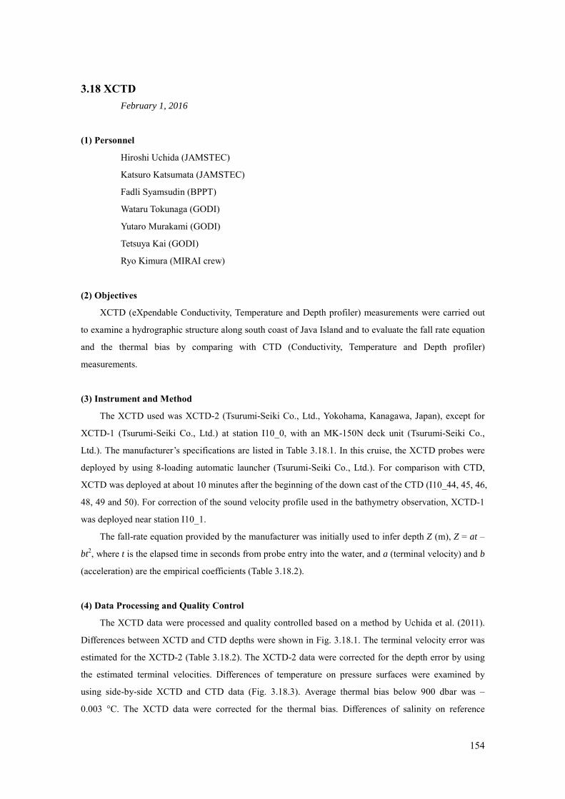
154
3.18 XCTD February 1, 2016
(1) Personnel
Hiroshi Uchida (JAMSTEC)
Katsuro Katsumata (JAMSTEC)
Fadli Syamsudin (BPPT)
Wataru Tokunaga (GODI)
Yutaro Murakami (GODI)
Tetsuya Kai (GODI)
Ryo Kimura (MIRAI crew)
(2) Objectives
XCTD (eXpendable Conductivity, Temperature and Depth profiler) measurements were carried out
to examine a hydrographic structure along south coast of Java Island and to evaluate the fall rate equation
and the thermal bias by comparing with CTD (Conductivity, Temperature and Depth profiler)
measurements.
(3) Instrument and Method
The XCTD used was XCTD-2 (Tsurumi-Seiki Co., Ltd., Yokohama, Kanagawa, Japan), except for
XCTD-1 (Tsurumi-Seiki Co., Ltd.) at station I10_0, with an MK-150N deck unit (Tsurumi-Seiki Co.,
Ltd.). The manufacturer’s specifications are listed in Table 3.18.1. In this cruise, the XCTD probes were
deployed by using 8-loading automatic launcher (Tsurumi-Seiki Co., Ltd.). For comparison with CTD,
XCTD was deployed at about 10 minutes after the beginning of the down cast of the CTD (I10_44, 45, 46,
48, 49 and 50). For correction of the sound velocity profile used in the bathymetry observation, XCTD-1
was deployed near station I10_1.
The fall-rate equation provided by the manufacturer was initially used to infer depth Z (m), Z = at –
bt2, where t is the elapsed time in seconds from probe entry into the water, and a (terminal velocity) and b
(acceleration) are the empirical coefficients (Table 3.18.2).
(4) Data Processing and Quality Control
The XCTD data were processed and quality controlled based on a method by Uchida et al. (2011).
Differences between XCTD and CTD depths were shown in Fig. 3.18.1. The terminal velocity error was
estimated for the XCTD-2 (Table 3.18.2). The XCTD-2 data were corrected for the depth error by using
the estimated terminal velocities. Differences of temperature on pressure surfaces were examined by
using side-by-side XCTD and CTD data (Fig. 3.18.3). Average thermal bias below 900 dbar was –
0.003 °C. The XCTD data were corrected for the thermal bias. Differences of salinity on reference

155
temperature surfaces were examined by using CTD data (Fig. 3.18.4). The XCTD data were corrected for
the estimated salinity bias.
(5) Results
Temperature-salinity plot using the quality controlled XCTD data is shown in Fig. 3.18.3. Potential
temperature cross section is shown in Fig. 3.18.4.
(6) References
Kizu, S., H. Onishi, T. Suga, K. Hanawa, T. Watanabe, and H. Iwamiya (2008): Evaluation of the fall
rates of the present and developmental XCTDs. Deep-Sea Res I, 55, 571–586.
Uchida, H., K. Shimada, and T. Kawano (2011): A method for data processing to obtain high-quality
XCTD data. J. Atmos. Oceanic Technol., 28, 816–826.
Uchida, H., A. Murata, and T. Doi (eds.) (2014): WHP P10 Revisit in 2011 Data Book, 179 pp.,
JAMSTEC.
Uchida, H., K. Katsumata, and T. Doi (eds.) (2015): WHP P14S/S04I Revisit in 2012/2013 Data Book,
187 pp., JAMSTEC.
Uchida, H and T. Doi (eds.) (2016): WHP P01 Revisit in 2014 Data Book (in prep.)
Table 3.18.1. Manufacturer’s specifications of XCTD-2.
-------------------------------------------------------------------------------------------------------------------------------
Parameter Range Accuracy
-------------------------------------------------------------------------------------------------------------------------------
Conductivity 0 ~ 60 mS cm–1 ±0.03 mS cm–1
Temperature –2 ~ 35 °C ±0.02 °C
Depth 0 ~ 1850 m 5 m or 2%, whichever is greater *
-------------------------------------------------------------------------------------------------------------------------------
* Depth error is shown in Kizu et al (2008).
Table 3.18.2. Manufacturer’s coefficients for the fall-rate equation.
-------------------------------------------------------------------------------------------------------------------------------
Model a (terminal velocity, m/s) b (acceleration, m/s2) e (terminal velocity
error, m/s)
-------------------------------------------------------------------------------------------------------------------------------
XCTD-4 3.43898 0.00031 –0.0198
-------------------------------------------------------------------------------------------------------------------------------
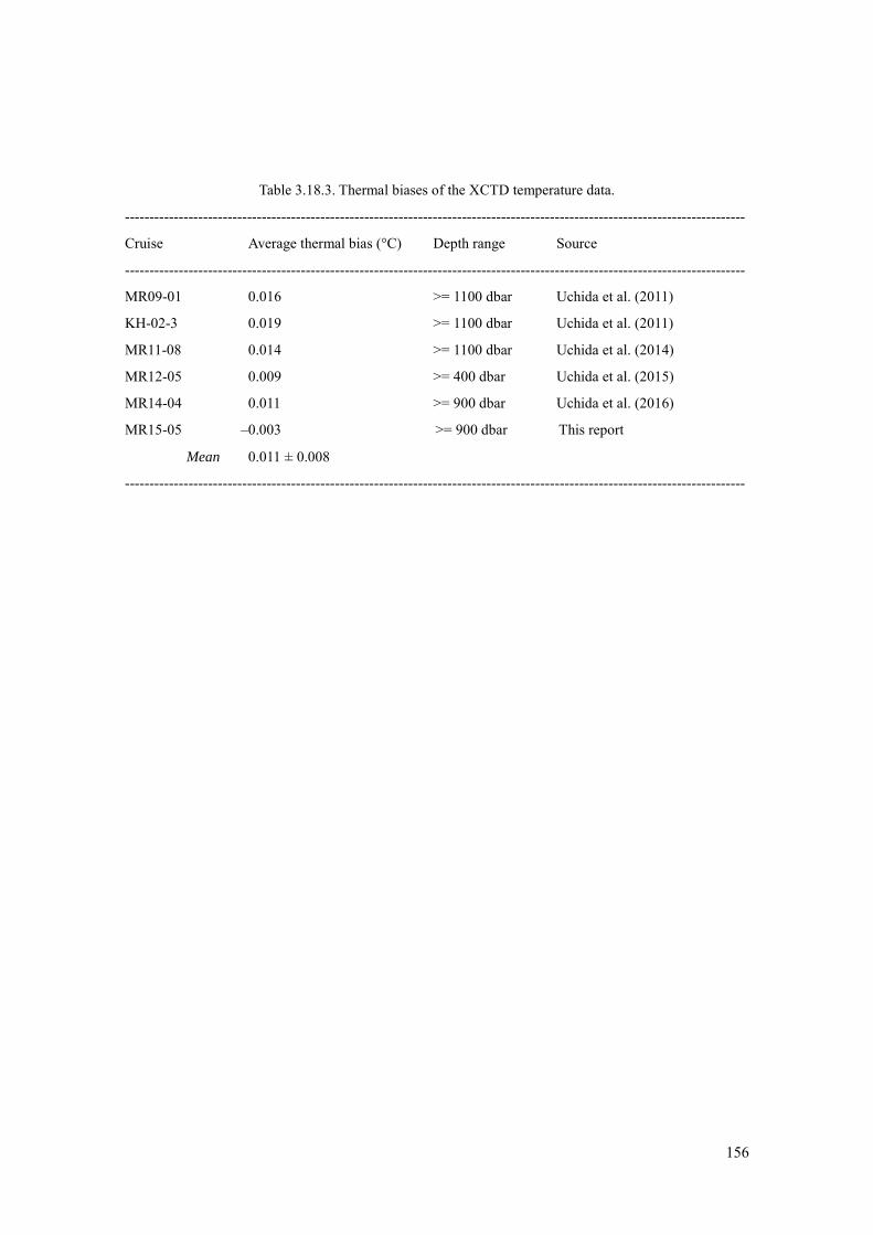
156
Table 3.18.3. Thermal biases of the XCTD temperature data.
-------------------------------------------------------------------------------------------------------------------------------
Cruise Average thermal bias (°C) Depth range Source
-------------------------------------------------------------------------------------------------------------------------------
MR09-01 0.016 >= 1100 dbar Uchida et al. (2011)
KH-02-3 0.019 >= 1100 dbar Uchida et al. (2011)
MR11-08 0.014 >= 1100 dbar Uchida et al. (2014)
MR12-05 0.009 >= 400 dbar Uchida et al. (2015)
MR14-04 0.011 >= 900 dbar Uchida et al. (2016)
MR15-05 –0.003 >= 900 dbar This report
Mean 0.011 ± 0.008
-------------------------------------------------------------------------------------------------------------------------------

157
Table 3.18.4. Salinity biases of the XCTD data.
-------------------------------------------------------------------------------------------------------------------------------
XCTD station Salinity bias Reference Reference Reference
temperature (°C) salinity CTD stations
-------------------------------------------------------------------------------------------------------------------------------
44 –0.008 3.0 34.7209 44,45,46,48,49,50
45 –0.003 3.0 34.7209 44,45,46,48,49,50
46 –0.022 3.0 34.7209 44,45,46,48,49,50
48 –0.016 3.0 34.7209 44,45,46,48,49,50
49 –0.015 3.0 34.7209 44,45,46,48,49,50
50 –0.010 3.0 34.7209 44,45,46,48,49,50
901 –0.035 6.0 34.6558 51
902 –0.034 4.2 34.6532 44,45,46,48,49,50
903 –0.023 4.2 34.6532 44,45,46,48,49,50
904 –0.040 3.0 34.7209 44,45,46,48,49,50
905 –0.034 3.0 34.7209 44,45,46,48,49,50
906 –0.035 3.0 34.7209 44,45,46,48,49,50
907 –0.033 3.0 34.7209 44,45,46,48,49,50
908 –0.030 3.0 34.7209 44,45,46,48,49,50
909 –0.042 3.0 34.7209 44,45,46,48,49,50
910 –0.022 3.0 34.7209 44,45,46,48,49,50
911 –0.022 3.0 34.7209 44,45,46,48,49,50
912 –0.037 3.0 34.7209 44,45,46,48,49,50
913 –0.035 4.2 34.6532 44,45,46,48,49,50
-------------------------------------------------------------------------------------------------------------------------------

158
Figure 3.18.1. Differences between XCTD and CTD depths for XCTD-2. Differences were estimated
with the same method as Uchida et al. (2011). Standard deviation of the estimates (horizontal bars) and
the manufacturer’s specification for XCTD depth error (dotted lines) are shown. The regression for the
data (solid line) is also shown.
Figure 3.18.2. Comparison between XCTD and CTD temperature profiles. (a) Mean temperature of CTD
profiles with standard deviation (shade) and (b) mean temperature difference with standard deviation

159
(shade) between the XCTD and CTD. Mean profiles were low-pass filtered by a running mean with a
window of 51 dbar.
Figure 3.18.3. Comparison of temperature-salinity profiles of CTD data (red lines) used for the XCTD
salinity bias estimation and salinity bias-corrected XCTD data (black lines).

160
Figure 3.18.4. Potential temperature (˚C) section along south coast of Java Island.

161
3.19 Micro Rider
- (1) Personnel
Shinya Kouketsu (JAMSTEC)
Hiroshi Uchida (JAMSTEC)
Katsurou Katsumata (JAMSTEC)
Ichiro Yasuda (AORI)
- (2) Objective
Microstructure observations to evaluate vertical mixing.
- (3) Instruments and method
Micro structure observations were carried out by micro-Rider 6000 (MR6000; Rockland
Scientific International Inc.), which is mounted CTD rosette and is powered from SBE 9plus.
We mounted two FP07 thermistors to obtain the high-frequency changes in temperature. We
sometimes replaced the probes during this cruise, as the probes didn’t work well. The
high-frequency pressure and acceleration profiles are also obtained by the sensors in MR6000.
The low-frequency profiles of temperature are archived in the MR6000 from the cables
connected with SBE-3 sensor on the CTD system. We download the profile data from the
MR6000 a cast. During this cruise, as we attached a bottom contact detector in some casts
(Stations 001, 002, and 013), the string and weight with the detector may affect the
microstructure measurements. After the cruise, we plan to examine the methods of the
correction and measurement quality evaluation with the comparison among the micro
temperature with CTD rosette, those with free fall instruments, and free fall micro shear
structure observations.
- (4) Micro-Temperature measurement history
– Station 001-030: T1111 and T1112
– Station 031-052: T1114 and T1115

4. Floats, Drifters, and Moorings 4.1 Argo floats (1) Personnel
Katsuro Katsumata (JAMSTEC)
Ann Thresher (CSIRO) not onboard
Mizue Hirano (JAMSTEC) not onboard
Shungo Oshitani (MWJ) Technical Staff
Shinsuke Toyoda (MWJ) Technical Staff (2) Objectives Now Argo floats are one of the core components of the Global Ocean Observing System http://www.ioc-goos.org/). The data from these floats are indispensable for both operational and scientific purposes. We contribute to the maintenance of this system by deploying new floats. (3) Deployments The floats usually drift at a depth of 1000 dbar (called the parking depth), diving to a depth of 2000 dbar and rising up to the sea surface by decreasing and increasing their volume and thus changing the buoyancy in ten-day cycles. During the ascent, they measure temperature, salinity, and pressure. They stay at the sea surface, transmitting the CTD data to the land and then return to the parking depth by decreasing volume. These floats measure temperature, salinity, and pressure. Detail of deployments is shown in Table 4.1.1. Table 4.1.1 Argo floats
Time Location CTD
station, if
avalable
Water Depth
(m)
Serial
Number
(Hull)
WMO ID
24 Dec 2015, 00:34 8-14.84S, 105-31.45E - 3410 7435 5905006
24 Dec 2015, 07:36 9-29.74S, 106-2.96E - 6258 7426 5905007
24 Dec 2015, 15:33 10-45.06S, 106-35.02E - 5855 6542 5905008
25 Dec 2015, 04:38 12-30.15S, 107-20.25E Station 900 4668 7041 5905009
25 Dec 2015, 14:13 14-15.04S, 108-5.04E - 5331 7042 5905010
31 Dec 2015, 15:18 20-28.37S, 110-55.37E Station 18 3673 7040 5905011
1 Jan 2016, 14:57 18-31.68S, 110-5.57E Station 22 4737 7039 5905012
2 Jan 2016, 21:36 16-19.92S, 111-16.59E Station 27 5186 7430 5905013
4 Jan 2016, 04:04 14-52.02S, 111-23.75E Station 31 5682 7431 5905014
4 Jan 2016, 19:25 14-8.15S, 111-35.04E Station 33 5650 7429 5905015
5 Jan 2016, 14:13 12-41.08S, 111-27.15E Station 36 3868 7428 5905016
7 Jan 2016, 01:56 10-57.86S, 111-44.82E Station 42 4606 7432 5905017
7 Jan 2016, 23:40 10-2.72S, 111-49.84E Station 46 2122 7427 5905018

163
8 Jan 2016, 12:00 9-14.05S, 111-54.13E Station 49 3045 7434 5905019
10 Jan 2016, 00:55 9-9.68S, 113-49.97E - 2232 7425 5905020
10 Jan 2016, 21:55 9-9.91S, 115-14.77E - 3095 7433 5905021
Leg 2
19 Jan 2016, 23:03 21-59.84N, 134-59.91E - 5462 OIN
11JAP-ARI-01
5901937
Sixteen floats (Teledyne Webb Research) deployed during Leg 1 were purchased by Marine and Atmospheric Research
CSIRO, transported by air from Australia to Japan, and loaded to R/V Mirai at Hachinohe on 6 Nov 2015. Before loading,
all floats went through pre-deployment tests. These floats were deployed from the stern of the vessel using the
harness-and-cardboard deployment system. After deployment, water pressure triggers internal electrical switch of the
floats. The trigger of the deployment system for two floats (S/N 7040 and 7429) failed so that these floats were deployed
using traditional snap-ring shackle. At CTD stations, floats were deployed just after the CTD/sampler system is recovered
on deck.
The float deployed during Leg 2 (Arvor –I, nke Instrumentation) was purchased by JAMSTEC. The float was activated
using magnetic switch and deployed from the stern using snap-ring shackle.
(4) Data archive
The real-time data are provided to meteorological organizations, research institutes, and universities via Global
Data Assembly Center (GDAC: http://www.usgodae.org/argo/argo.html, http://www.coriolis.eu.org/) and Global Telecommunication System (GTS), and utilized for analysis and forecasts of sea conditions.

164
III. Notice on Using This cruise report is a preliminary documentation as of the end of the cruise. This report may not be corrected even if changes on contents (i.e. taxonomic classifications) may be found after its
publication. This report may also be changed without notice. Data on the cruise report may be raw or unprocessed. If you are going to use or refer to the data written on this report, please ask the Chief Scientist for latest information.
Users of data or results on this cruise report are requested to submit their results to the Data Management Group of
JAMSTEC.

165
Recommended


![R/V MIRAI Cruise Report MR02-K06 Leg-1...R/V Mirai Cruise Report MR02-K06 Leg-1 [Contents] 1. Introduction 2. Cruise Summary 3. List of Instruments 4. Cruise Track and Log 5. List](https://img.pdfslide.us/doc/110x75/5e3c53335b0f2f1153740a02/rv-mirai-cruise-report-mr02-k06-leg-1-rv-mirai-cruise-report-mr02-k06-leg-1.jpg)