Rolling Shutter Camera Relative Pose: Generalized Epipolar Geometry

Yuchao Dai1, Hongdong Li1,2 and Laurent Kneip1,2

1 Research School of Engineering, Australian National University2ARC Centre of Excellence for Robotic Vision (ACRV)

Abstract

The vast majority of modern consumer-grade cameras

employ a rolling shutter mechanism. In dynamic geomet-

ric computer vision applications such as visual SLAM, the

so-called rolling shutter effect therefore needs to be prop-

erly taken into account. A dedicated relative pose solver

appears to be the first problem to solve, as it is of eminent

importance to bootstrap any derivation of multi-view ge-

ometry. However, despite its significance, it has received

inadequate attention to date.

This paper presents a detailed investigation of the ge-

ometry of the rolling shutter relative pose problem. We in-

troduce the rolling shutter essential matrix, and establish

its link to existing models such as the push-broom cameras,

summarized in a clean hierarchy of multi-perspective cam-

eras. The generalization of well-established concepts from

epipolar geometry is completed by a definition of the Samp-

son distance in the rolling shutter case. The work is con-

cluded with a careful investigation of the introduced epipo-

lar geometry for rolling shutter cameras on several dedi-

cated benchmarks.

1. Introduction

Rolling-Shutter (RS) CMOS cameras are getting more

and more popularly used in real-world computer vision ap-

plications due to their low cost and simplicity in design. To

use these cameras in 3D geometric computer vision tasks

(such as 3D reconstruction, object pose, visual SLAM), the

rolling shutter effect (e.g. wobbling) must be carefully ac-

counted for. Simply ignoring this effect and relying on a

global-shutter method may lead to erroneous, undesirable

and distorted results (e.g. [11, 13, 3]).

Recently, many 3D vision algorithms have been adapted

to the rolling shutter case (e.g. absolute Pose [15] [3] [22],

Bundle Adjustment [9], and stereo rectification [21]). Quite

surprisingly, no previous attempt has been reported on solv-

ing the relative pose problem with a RS camera.

The complexity of this problem stems from the fact that

an RS camera does not satisfy the pinhole projection model,

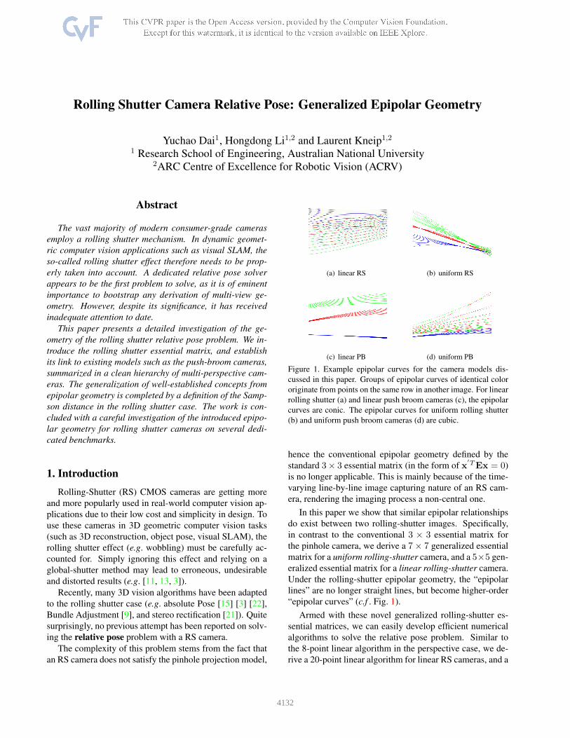
(a) linear RS (b) uniform RS

(c) linear PB (d) uniform PB

Figure 1. Example epipolar curves for the camera models dis-

cussed in this paper. Groups of epipolar curves of identical color

originate from points on the same row in another image. For linear

rolling shutter (a) and linear push broom cameras (c), the epipolar

curves are conic. The epipolar curves for uniform rolling shutter

(b) and uniform push broom cameras (d) are cubic.

hence the conventional epipolar geometry defined by the

standard 3× 3 essential matrix (in the form of x′TEx = 0)

is no longer applicable. This is mainly because of the time-

varying line-by-line image capturing nature of an RS cam-

era, rendering the imaging process a non-central one.

In this paper we show that similar epipolar relationships

do exist between two rolling-shutter images. Specifically,

in contrast to the conventional 3 × 3 essential matrix for

the pinhole camera, we derive a 7× 7 generalized essential

matrix for a uniform rolling-shutter camera, and a 5×5 gen-

eralized essential matrix for a linear rolling-shutter camera.

Under the rolling-shutter epipolar geometry, the “epipolar

lines” are no longer straight lines, but become higher-order

“epipolar curves” (c.f . Fig. 1).

Armed with these novel generalized rolling-shutter es-

sential matrices, we can easily develop efficient numerical

algorithms to solve the relative pose problem. Similar to

the 8-point linear algorithm in the perspective case, we de-

rive a 20-point linear algorithm for linear RS cameras, and a

4132

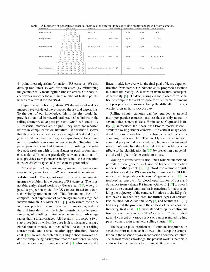
Table 1. A hierarchy of generalized essential matrices for different types of rolling-shutter and push-broom cameras.Camera Model Essential Matrix Monomials Degree-of-freedom Linear Algorithm Non-linear Algorithm Motion Parameters

Perspective camera

f11 f12 f13f21 f22 f23f31 f32 f33

(ui, vi, 1) 32 = 9 8-point 5-point R, t

Linear push broom

0 0 f13 f140 0 f23 f24f31 f32 f33 f34f41 f42 f43 f44

(uivi, ui, vi, 1) 12 = 42 − 22 11-point 11-point R, t,d1,d2

Linear rolling shutter

0 0 f13 f14 f150 0 f23 f24 f25f31 f32 f33 f34 f35f41 f42 f43 f44 f45f51 f52 f53 f54 f55

(u2

i , uivi, ui, vi, 1) 21 = 52 − 22 20-point 11-point R, t,d1,d2

Uniform push broom

0 0 f13 f14 f15 f160 0 f23 f24 f25 f26f31 f32 f33 f34 f35 f36f41 f42 f43 f44 f45 f46f51 f52 f53 f54 f55 f56f61 f62 f63 f64 f65 f66

(u2

i vi, u2

i , uivi, ui, vi, 1) 32 = 62 − 22 31-point 17-point R, t,w1,w2,d1,d2

Uniform rolling shutter

0 0 f13 f14 f15 f16 f170 0 f23 f24 f25 f26 f27f31 f32 f33 f34 f35 f36 f37f41 f42 f43 f44 f45 f46 f47f51 f52 f53 f54 f55 f56 f57f61 f62 f63 f64 f65 f66 f67f71 f72 f73 f74 f75 f76 f77

(u3

i , u2

i vi, u2

i , uivi, ui, vi, 1) 45 = 72 − 22 44-point 17-point R, t,w1,w2,d1,d2

44-point linear algorithm for uniform RS cameras. We also

develop non-linear solvers for both cases (by minimizing

the geometrically meaningful Sampson error). Our nonlin-

ear solvers work for the minimum number of feature points,

hence are relevant for RANSAC.

Experiments on both synthetic RS datasets and real RS

images have validated the proposed theory and algorithms.

To the best of our knowledge, this is the first work that

provides a unified framework and practical solutions to the

rolling shutter relative pose problem. Our 5 × 5 and 7 × 7RS essential matrices are original; they were not reported

before in computer vision literature. We further discover

that there also exist practically meaningful 4× 4 and 6× 6generalized essential matrices, corresponding to linear, and

uniform push-broom cameras, respectively. Together, this

paper provides a unified framework for solving the rela-

tive pose problem with rolling-shutter or push-broom cam-

eras under different yet practically relevant conditions. It

also provides new geometric insights into the connection

between different types of novel camera geometries.

Table-1 gives a brief summary of the new results discov-

ered in this paper. Details will be explained in Section-4.

Related work: The present work discusses a fundamental

geometric problem in the context of RS cameras. The most

notable, early related work is by Geyer et al. [16], who pro-

posed a projection model for RS cameras based on a con-

stant velocity motion model. This fundamental idea of a

compact, local expression of camera dynamics has regained

interest through Ait-Aider et al. [1], who solved the abso-

lute pose problem through iterative minimization, and for

the first time described the higher density of the temporal

sampling of a rolling shutter mechanism as an advantage

rather than a disadvantage. Albl et al.[3] proposed a two-

step procedure in which the pose is first initialized using a

global shutter model, and then refined based on a rolling

shutter model and a small-rotation approximation. Saurer

et al. [22] solved the problem in a single shot, however un-

der the simplifying assumption that the rotational velocity

of the camera is zero. Sunghoon et al. [11] also employed a

linear model, however with the final goal of dense depth es-

timation from stereo. Grundmann et al. proposed a method

to automatic rectify RS distortion from feature correspon-

dences only [5]. To date, a single-shot, closed-form solu-

tion to compute the relative pose for a RS camera remains

an open problem, thus underlining the difficulty of the ge-

ometry even in the first-order case.

Rolling shutter cameras can be regarded as general

multi-perspective cameras, and are thus closely related to

several other camera models. For instance, Gupta and Hart-

ley [6] introduced the linear push-broom model where—

similar to rolling shutter cameras—the vertical image coor-

dinate becomes correlated to the time at which the corre-

sponding row is sampled. This notably leads to a quadratic

essential polynomial and a related, higher-order essential

matrix. We establish the close link to this model and con-

tribute to the classification in [27] by presenting a novel hi-

erarchy of higher order essential matrices.

Moving towards iterative non-linear refinement methods

permits a more general inclusion of higher-order motion

models. Hedborg et al. [9, 10] introduced a bundle adjust-

ment framework for RS cameras by relying on the SLERP

model for interpolating rotations. Magarand et al. [15] in-

troduced an approach for global optimization of pose and

dynamics from a single RS image. Oth et al. [17] proposed

to use more general temporal basis functions for parameter-

izing the trajectory of the camera. Solutions to the RS prob-

lem have also been explored for further types of sensors.

For instance, Ait-Aider and Berry [2] and Saurer et al. [21]

had anaylzed the problem in the context of stereo cameras.

Recently, Kerl et al. [13] have started to apply continuous

time parametrizations to RGB-D cameras. Ponce studied

general concept of various types of cameras including line

pencil camera akin to general rolling shutter [20].

The relative pose problem is of eminent importance in

structure-from-motion, as it allows to bootstrap the compu-

tation in the absence of any information about the structure.

To the best of our knowledge, the present work is the first to

address it in the context of a rolling shutter camera.

4133

2. Rolling-Shutter Camera Models

A critical difference between a RS camera and a pin-

hole camera is that the former does no longer possess a

single center-of-projection in the general case. Instead, in

a rolling-shutter image, each of its scanlines generally has

a different effective projection center (temporal-dynamic)

as well as a different local frame and orientation.

In an attempt to present this matter from a mathemat-

ical perspective, let us start with re-examining the model

of a (global shutter) pinhole camera, which can be entirely

described by a central projection matrix: P = K[R, t].When an RS camera is in motion during image acquisition,

all its scanlines are sequentially exposed at different time

steps; hence each scanline possesses a different local frame.

Mathematically, we need to assign a unique projection ma-

trix to every scanline in an RS image Pui= K[Rui

, tui].

General Rolling Shutter Camera. It is common to as-

sume that the motion of a rolling-shutter camera during im-

age acquisition is smooth. Otherwise an arbitrarily non-

smoothly moving RS camera would create meaningless im-

ages suffering from arbitrary fragmentations.

Therefore, a smoothly moving RS camera is considered

as the most general form of rolling-shutter models. It is easy

to see that for a general RS image its scanlines’ local pose

matrices P0,P1,P2, · · · ,PN−1 will trace out a smooth

trajectory in the SE(3) space. B-splines have been used to

model this trajectory in the RS context [24, 18][13].

To ease the derivation, we assume the RS camera is in-

trinsically calibrated. However, note that many of the re-

sults presented in this paper remain extendable to the un-

calibrated case as well (by transitioning from the essential

matrix to the corresponding fundamental matrix). Also note

that the task of intrinsic calibration can be easily done, e.g.

by applying any standard camera calibration procedure to

still imagery taken by an RS camera.

Linear Rolling-Shutter Camera. The motion of the

camera is a pure translation by a constant linear velocity.

The orientations of local scanline frames are constant. In

this case, the projection centers of the scanlines lie on a

straight line in 3D space. Supposing that constant velocity

induces a translation shift of d per image row (expressed in

normalized coordinates), we can write down the ui-th pro-

jection matrix as

Pui= [R0, t0 + uid]. (1)

We use the top-most scanline’s local frame [R0, t0] as the

reference frame of the RS image.

Uniform Rolling-Shutter Camera. The uniform rolling-

shutter camera is another popular RS model, which is more

general than the linear RS model. The camera is performing

a uniform rotation at a constant angular velocity, in addition

to a uniform linear translation at constant linear velocity.

All the centers of projection form a helix spiral trajectory.

We use d ∈ R3 to denote the constant linear velocity and

w ∈ R3 for the constant angular velocity (expressing angu-

lar displacement per row). Let w be parametrized in the

angle-axis representation (i.e. w = ω[n]). The ui-th scan-

line’s local projection matrix is Pui= [Rui

, tui], where

Rui=(I+ sin(uiω)[n]× + (1− cos(uiω)) [n]

2×)R0,

tui=t0 + uid. (2)

One may further assume that the inter-scanline rotation dur-

ing image acquisition is very small. This is a reasonable as-

sumption, as the acquisition time for a single image is very

short, often in the order of 10s milliseconds, and the motion

of an RS camera is typically small. Under the small-rotation

approximation, we have

Rui=(I+ uiω[n]×)R0,

tui=t0 + uid. (3)

3. The Rolling Shutter Relative Pose Problem

The RS Relative Pose problem consists of finding the

relative camera displacement between two RS views, given

image feature correspondences.

It is well known that for the perspective case the epipo-

lar geometry plays a central role in relative pose estimation,

translated into a simple 3-by-3 matrix called the essential

(or fundamental) matrix. Specifically, given a set of corre-

spondences between two views, xi = [ui, vi, 1]T ↔ x

′

i =[u′

i, v′

i, 1]T , we have the standard essential matrix con-

straint: x′Ti Exi = 0. From a sufficient number of corre-

spondences one can solve for E. Decomposing E according

to E = [t]×R leads to the relative pose (i.e. R and t).

For a rolling-shutter camera, unfortunately, such a global

3-by-3 essential matrix does not exist. This is primarily be-

cause an RS camera is not a central projection camera; every

scanline has its own distinct local pose. As a result, every

pair of feature correspondences may give rise to a different

“essential matrix”. Formally, for xi ↔ x′

i, we have

x′Ti Eui,u

′

ixi = 0. (4)

Note that E is dependent of the scanlines ui and u′

i. In other

words, there does not exist a single global 3 × 3 essential

matrix for a pair of RS images.

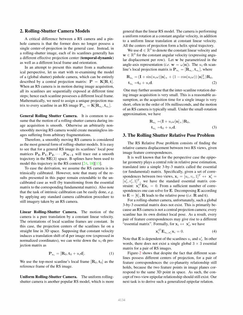
Figure-2 shows that despite the fact that different scan-

lines possess different centers of projection, for a pair of

feature correspondences the co-planarity relationship still

holds, because the two feature points in image planes cor-

respond to the same 3D point in space. As such, the con-

cept of two-view epipolar relationship should still exist. Our

next task is to derive such a generalized epipolar relation.

4134

Figure 2. This figure shows that different scanlines in a RS image

have different effective optical centers. For any pair of feature cor-

respondences (indicated by red ‘x’s in the picture), a co-planarity

relationship however still holds.

Given two scanlines ui, uj and the corresponding camera

poses Pui= [Rui

, tui] and Puj

= [Ruj, tuj

], we have

Euiuj= [tuj

−RujR

Tuitui

]×RujR

Tui. (5)

Rolling Shutter Relative Pose. Note, given a pair of fea-

ture correspondences xi ↔ x′

i, one can establish the fol-

lowing RS epipolar equation: x′Ti Euiu

′

ixi = 0. Given suffi-

cient pairs of correspondences; each pair contributes to one

equation over the unknown parameters; our goal is to solve

for the relative pose between the two RS images.

We set the first camera’s pose at [I,0], and the second

camera at [R, t]. We denote the two cameras’ inter-scanline

rotational (angular) velocities as w1, and w2, and their lin-

ear translation velocities as d1 and d2. Taking a uniform RS

camera as an example, the task of finding the relative pose is

to find the unknowns {R, t,w1,w2,d1,d2}. In total there

are 2 × 12 − 6 − 1 = 17 non-trivial variables (excluding

the gauge freedom of the first camera, and a global scale).

Collecting at least 17 equations in general configuration,

it is possible to solve this system of (generally nonlinear)

equations over the 17 unknown parameters. In this paper,

we will show how to derive linear N-point algorithms for

rolling shutter cameras, as an analogy to the linear 8-point

algorithm for the case of a pinhole camera.

4. Rolling-Shutter Essential Matrices

In this section, we will generalize the conventional 3× 3essential matrix for perspective cameras to 4×4, 5×5, 6×6,and 7 × 7 matrices for different types of Rolling-Shutter

(RS) and Push-Broom (PB) cameras. The reason for in-

cluding push-broom cameras will be made clear soon.

4.1. A 5× 5 essential matrix for linear RS cameras

For a linear rolling shutter camera, since the inter-

scanline motion is a pure translation, there are four parame-

ter vectors to be estimated, namely{R, t,d1,d2}. The total

degree of freedom of the unknowns is 3+3+3+3−1 = 11.

(the last ‘-1’ accounts for a global scale).

The epipolarity defined between the ui-th scanline of the

first RS frame and the u′

i-th scanline of the second RS frame

is represented as Euiu′

i= [tuiu

′

i]×Ruiu

′

i, where the trans-

lation tuiu′

i= t+ u′

id2 − uiRd1. This translates into

u′

i

v′i1

T

[t+ u′

id2 − uiRd1]×R

ui

vi1

= 0. (6)

Expanding this scanline epipolar equation, one can obtainthe following 5× 5 matrix form:

u′2

i

u′

iv′

i

u′

i

v′

i

1

T

0 0 f13 f14 f150 0 f23 f24 f25f31 f32 f33 f34 f35f41 f42 f43 f44 f45f51 f52 f53 f54 f55

u2

i

uiviui

vi1

= 0,

(7)

where the entries of the 5×5 matrix F = [fi,j ] are functions

of the 11 unknown parameters {R, t,d1,d2}. In total, there

are 21 homogeneous variables, thus a linear 20-point solver

must exist to solve for this hyperbolic essential matrix.

By redefining d1 ← Rd1, we easily obtain

Euiu′

i= ([t]× + u′

i[d2]× − ui[d1]×)R. (8)

Denoting E0 = [t]×R, E1 = [d1]×R and E2 = [d2]×R,

we have:

[u′

i, v′

i, 1](E0 + u′

iE2 − uiE1)[ui, vi, 1]T = 0. (9)

The 5× 5 matrix F is defined in the following way

F =

0 0 E1,11 E1,21 E1,31

0 0 E1,12 E1,22 E1,32

E2,11 E2,21 a b c

E2,12 E2,22 E0,12 + E2,32 E0,22 E0,32

E2,13 E2,23 E0,13 + E2,33 E0,23 E0,33

, (10)

where a = E0,11 + E1,13 + E2,31, b = E0,21 + E1,23, c =E0,31 + E1,33.Hyperbolic epipolar curves. Note that the “epipolar lines”

for a linear RS camera are hyperbolic curves. It is easy to

verify that the generalized essential matrix for linear rolling

shutter camera is full rank and the epipole lies in infinity.

Difference with axial camera The linear rolling shutter

camera give rise to an axis where every back-projection ray

intersects. However, the temporal-dynamic nature of lin-

ear rolling shutter camera distinguishes itself from the axial

camera [26], where the internal displacement (linear veloc-

ity) is unknown and to estimate. Even though our linear RS

essential matrix shares the same size as axial camera essen-

tial matrix [25], the detailed structure is different.

4.2. A 7×7 essential matrix for uniform RS cameras

Consider a uniform RS camera undergoing a rotation at

constant angular velocity w and a translation at constant

linear velocity d. We assume the angular velocity is very

4135

small. By using the small-rotation approximation,we have

the ui-th scanline’s local pose as

Pui= [(I+ ui[w]×)R0, t0 + uid]. (11)

Given a pair of two corresponding uniform RS cameraframes, we then have

[u′

i, v′

i , 1][t+u′

id2−uiRuiu′

i

d1]×Ruiu′

i

[ui, vi, 1]T = 0, (12)

Expanding this equation with the aid of the small rotation

approximation results in

Rui,u′

i= (I+ u′

i[w2]×)R0(I− ui[w1]×), (13)

and we finally obtain:[

u′3

i , u′2

i v′i, u′2

i , u′

iv′

i, u′

i, v′

i, 1]

F[

u3

i , u2

i vi, u2

i , uivi, ui, vi, 1]T

= 0,

(14)

where

F =

0 0 f13 f14 f15 f16 f170 0 f23 f24 f25 f26 f27f31 f32 f33 f34 f35 f36 f37f41 f42 f43 f44 f45 f46 f47f51 f52 f53 f54 f55 f56 f57f61 f62 f63 f64 f65 f66 f67f71 f72 f73 f74 f75 f76 f77

.

This gives a 7 × 7 RS essential matrix F, whose

elements are functions of the 18 unknowns (i.e.

{R, t,w1,w2,d1,d2}). Also note the induced epipolar

curves are cubic. In total there are 45 homogeneous vari-

ables, thus a 44-point linear algorithm exists to solve for

this hyperbolic essential matrix. The generalized essential

matrix for uniform rolling shutter camera is full rank and

the epipole lies in infinity.

If w1 = w2 = 0, the equation will reduce to Eq.-(9).

This exactly reduces to the linear rolling shutter case.

4.3. A 4× 4 essential matrix for linear PB cameras

Researchers have previously noticed the similarity be-

tween a spacetime sweeping camera (such as RS) and a

push-broom camera [16, 23]. Here, we further illustrate this

similarity, via our high-order essential matrix.

Specifically, the above 5× 5 and 7× 7 RS essential ma-

trices have inspired us to explore further. Do 4× 4 or 6× 6generalized essential matrices also exist? Following a sim-

ilar approach, we quickly find out that: these two general-

ized essential matrices do exist and they each corresponds

to a special type of push-broom camera.For linear push-broom (PB) cameras (as defined in [6]),

there exists a 4× 4 essential matrix:

F =

0 0 f13 f140 0 f23 f24f31 f32 f33 f34f41 f42 f43 f44

. (15)

The resulting linear push-broom epipolar equation reads as

(u′

1v′

1, u′

1, v′

1, 1)F(u1v1, u1, v1, 1)T = 0. (16)

We must point out that this 4 × 4 linear PB essential ma-

trix result is not new; paper [6] already reported it though

via a different approach. This however precisely confirms

that our method provides a unified framework for handling

different types of novel, higher-order epipolar geometries,

including a PB camera.

Difference with X-slit camera The linear PB camera

give rise to two oblique slits setting, where one slit is the

line of center of projection and the other slit corresponds

to the viewing direction. However, the slit corresponds to

the moving camera projection center is unknown and to es-

timate. Although the linear PB essential matrix shares the

same size as the X-Slit camera essential matrix [25], the

detailed structure is different.

4.4. A 6×6 essential matrix for uniform PB cameras

Similarly, for the uniform PB camera where the viewplane of the camera is undergoing a uniform rotation be-sides its linear sweeping, we can easily derive a 6 × 6 uni-form PB essential matrix as:

u′2

i v′

i

u′2

i

u′

iv′

i

u′

i

v′

i

1

T

0 0 f13 f14 f15 f160 0 f23 f24 f25 f26f31 f32 f33 f34 f35 f36f41 f42 f43 f44 f45 f46f51 f52 f53 f54 f55 f56f61 f62 f63 f64 f65 f66

u2

i viu2

i

uiviui

vi1

= 0.

(17)

There are 32 variables in this PB essential matrix (6 × 6minus the top-left 2× 2 corner), suggesting that a 31-point

linear algorithm can be used to estimate F. Note also that

the resulting (generalized) epipolar curves are cubic.

RS camera VS PB camera: Both RS camera and PB

camera have a scanline dependent pose, i.e., temporal-

dynamic center of projection. For PB cameras, the scan-

line direction is fixed relative to the local coordinate while

the scanline direction changes relative to the local coordi-

nate for RS cameras. This creates the main difference be-

tween PB cameras and RS cameras and the extras freedom

explains the increased order of polynomials in expressing

the generalized epipolar geometry (4 VS 6 and 5 VS 7).

5. Linear N-point algorithms for RS cameras

Summary of the Above Results. The above results are

summarized in Table-1. We also include the number of

points needed to solve linearly for the respective general-

ized essential matrices. Next, let us use as an example the

linear RS camera to derive a linear 20-point algorithm for

solving the uniform RS essential matrix. The linear solu-

tions for other types of cameras in the table can be similarly

derived, hence are omitted here. Interested readers will find

more information in our supplementary material.

4136

5.1. A linear 20­point algorithm for RS cameras

For solving the linear RS relative pose problem, we first

solve for the 5 × 5 RS essential matrix F ∈ R5×5. Then

from its 21 non-zero elements, we recover the three atomic

essential matrices E0,E1 and E2. Finally, the relative pose

(R, t) and velocities d1,d2 can be simply extracted by de-

composing E0,E1 and E2.

5.1.1 Solving the 5× 5 linear RS essential matrix

The linear RS essential matrix F contains only 21 non-

trivial homogeneous variables, hence its degree of freedom

is 20. Collecting 20 correspondences, one can solve for the

5× 5 matrix F linearly by SVD.

5.1.2 Recovering atomic essential matrices

Once the 5 × 5 matrix F is found, our next goal is to re-

cover the individual atomic essential matrices E0,E1 and

E2. Eq.-(10) provides 21 linear equations on the three es-

sential matrices. As the three essential matrices consist

of 27 elements, we need six extra constraints to solve for

E0,E1 and E2. To this end, we resort to the inherent con-

straints on standard 3×3 essential matrices, e.g. det(E) = 0and 2EE

TE−Tr(EE

T )E = 0, since E0,E1 and E2 are

standard 3× 3 essential matrices.

A quadratic solution. Examining the relationship be-

tween the linear RS essential matrix and the atomic essential

matrices, we find that the right bottom 2 × 2 corner of E0

matrix can be directly read out; the first and second columns

of E1 can also be read out; the first and second rows of E2

are also available from the RS essential matrix F.

Taking E1 as an example, we now illustrate how to

complete its missing column from two recovered columns.

Once we have solved F, we can directly read out the

first two columns of E1, i.e. E1 =

E11

1E12

1∗

E21

1E22

1∗

E31

1E32

1∗

.

In order to recover the last missing column, we use

both of its rank-2 constraint and cubic constraints. First,

by using the rank-2 constraint we express the third col-

umn as a linear combination of the first two columns,

i.e.

[E13

E23

E33

]= λ1

[E11

E21

E31

]+ λ2

[E12

E22

E32

]. The remaining

nonlinear constraints on a 3 × 3 essential matrix pro-

vide 9 equations over λ1 and λ2, among which we need

to choose two in order to solve for λ1 and λ2. For

simplicity, we only choose two quadratic ones, namely{

a11λ2

1+ a12λ1λ2 + a13λ

2

2+ a14 = 0

a21λ2

1+ a22λ1λ2 + a23λ

2

2+ a24 = 0

. These quadratic

equations can be solved efficiently by using any off-the-

shelf solver. Following a similar procedure, we can also

solve for E2, and subsequently solve for E0.

5.1.3 Recovering relative pose and velocities

Given the three essential matrices E0 = [t]×R, E1 =[d1]×R, and E2 = [d2]×R, we decompose them into rela-

tive transformations (R, t) and velocities d1,d2 [8].

Other linear N-point algorithms can be similarly derived.

In solving the linear RS essential matrix F, we apply nor-

malization to the image coordinates and the lifted coordi-

nates (u2i , uivi, ui, vi, 1) in the way as in [7].

6. Nonlinear Solvers w/ Sampson Error

Based on the above generalized essential matrices,

we can now also devise nonlinear solvers. Instead of

minimizing an algebraic error, we minimize the ge-

ometrically more meaningful (generalized) Sampson

error metric. For example, in the case of a uniform

RS camera, the Sampson error is the first-order ap-

proximation of the distance between a (generalized)

feature vector xi = [u3i , u

2i vi, u

2i , uivi, ui, vi, 1]

T

and its corresponding RS epipolar curve, i.e.,

eSampson =∑n

i=1(x

′Ti Fxi)

2

∑7

j=1((Fxi)2j+(FTx

′

i)2j).

We envisage three scenarios where such nonlinearsolvers can prove useful:

a) Use it as a ‘gold-standard’ nonlinear refinement procedure.

b) Use it as a general solver which directly searches the variables.

c) Use it as a minimal-case solver together with RANSAC.

The last case is particularly relevant as RANSAC favors

smaller sample sizes. For example, for the case of uniform

RS camera our linear algorithm asks for 44 points; in con-

trast, a minimal-case solver only requires 17 points, as there

are in total 18 degrees of freedom in [R, t,w1,w2,d1,d2].To solve the above Sampson error minimization prob-

lem, we parametrize the rotation with its angle-axis repre-

sentation, then we use the standard unconstrained optimiza-

tion solver ‘fminunc’ in Matlab.

7. Experimental evaluation

We evaluated the linear and uniform RS rela-

tive pose methods on both synthetic and real image

datasets. When ground-truth data is available, error met-

rics for rotation and translation estimates are defined

as eR = acos((trace(R̂RTGT ) − 1)/2), and eT =

acos(t̂T tGT /(‖t̂‖‖tGT ‖)).

7.1. Simulation Experiments

Generating geometrically consistent simulation mea-

surements for a dynamic RS camera is a challenge in itself.

First, a relative pose (R, t) is randomly defined between the

image pair. The focal length is set to 640 while the image

resolution is defined to be 640 × 480. Second, given trans-

lation velocities d1 and d2, and angular velocities w1,w2,

4137

the camera pose for each row can be determined. The cor-

respondences are then simulated such that they are not too

far from what a real world image feature tracker would re-

turn. Each generation is finalized by a cheirality check to

guarantee the corresponding 3D point lies in front of both

cameras. All experiments are repeated 200 times to obtain

statistically relevant conclusions.

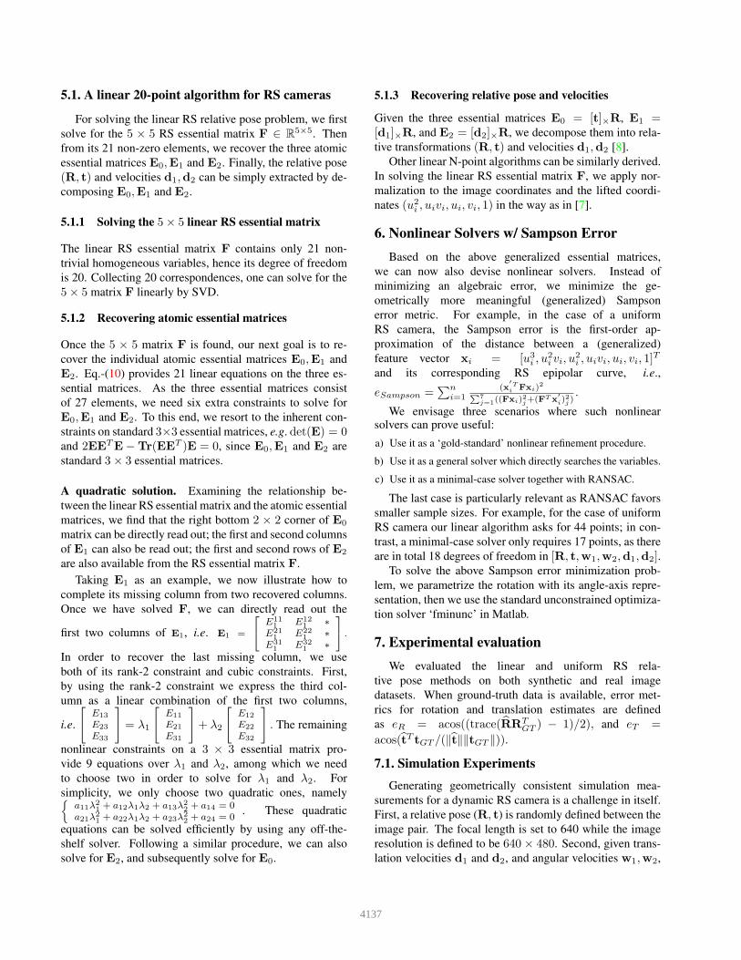
Evaluation of the linear methods. Here we first test our

20-point algorithm for linear RS relative pose. We use the

angle between vectorized ground truth and estimated essen-

tial matrices as a performance indicator. Fig. 3 illustrates

the essential matrix estimation error with respect to increas-

ing noise. The figure is using a double logarithmic scale.

For the 44-point algorithm, a similar curve could also be

obtained. We observe that the linear methods are very sensi-

tive to noise. To deal with real world noise, in the following

experiments, we used the nonlinear optimization method.

Figure 3. Evaluation on increasing Gaussian noise for linear 20-

point algorithm. Noise is added to the normalized coordinates.

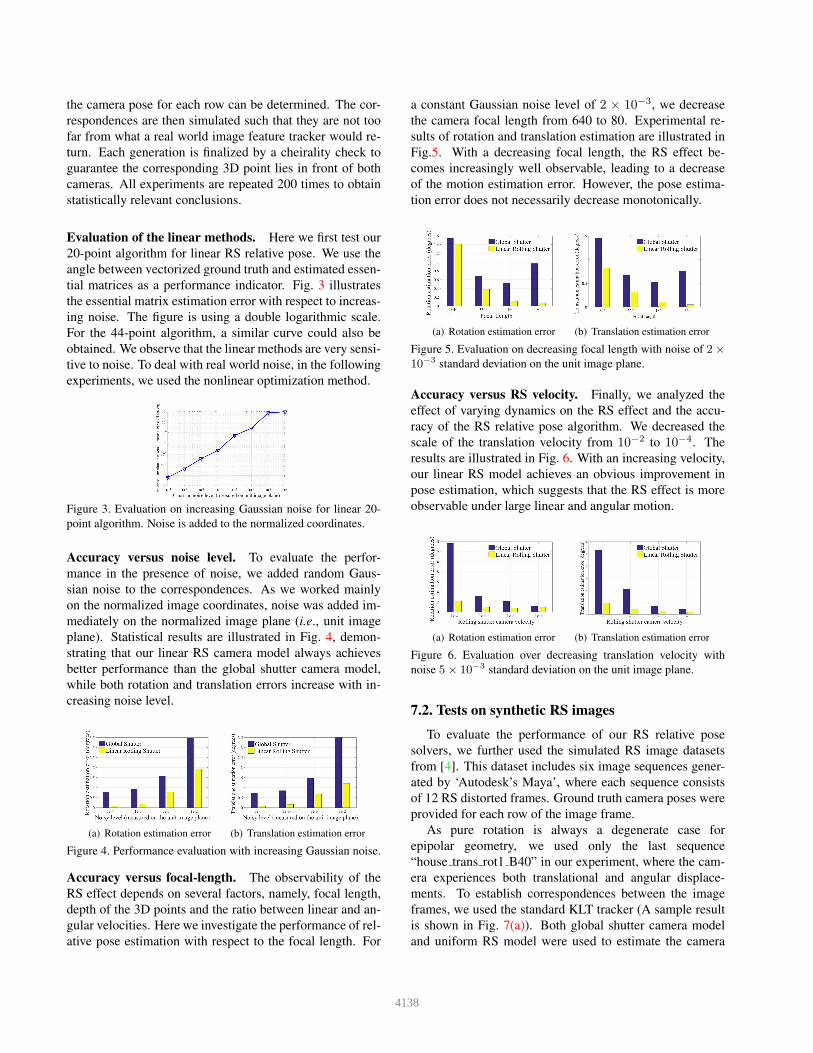
Accuracy versus noise level. To evaluate the perfor-

mance in the presence of noise, we added random Gaus-

sian noise to the correspondences. As we worked mainly

on the normalized image coordinates, noise was added im-

mediately on the normalized image plane (i.e., unit image

plane). Statistical results are illustrated in Fig. 4, demon-

strating that our linear RS camera model always achieves

better performance than the global shutter camera model,

while both rotation and translation errors increase with in-

creasing noise level.

(a) Rotation estimation error (b) Translation estimation error

Figure 4. Performance evaluation with increasing Gaussian noise.

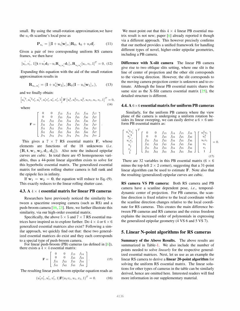
Accuracy versus focal-length. The observability of the

RS effect depends on several factors, namely, focal length,

depth of the 3D points and the ratio between linear and an-

gular velocities. Here we investigate the performance of rel-

ative pose estimation with respect to the focal length. For

a constant Gaussian noise level of 2 × 10−3, we decrease

the camera focal length from 640 to 80. Experimental re-

sults of rotation and translation estimation are illustrated in

Fig.5. With a decreasing focal length, the RS effect be-

comes increasingly well observable, leading to a decrease

of the motion estimation error. However, the pose estima-

tion error does not necessarily decrease monotonically.

(a) Rotation estimation error (b) Translation estimation error

Figure 5. Evaluation on decreasing focal length with noise of 2×

10−3 standard deviation on the unit image plane.

Accuracy versus RS velocity. Finally, we analyzed the

effect of varying dynamics on the RS effect and the accu-

racy of the RS relative pose algorithm. We decreased the

scale of the translation velocity from 10−2 to 10−4. The

results are illustrated in Fig. 6. With an increasing velocity,

our linear RS model achieves an obvious improvement in

pose estimation, which suggests that the RS effect is more

observable under large linear and angular motion.

(a) Rotation estimation error (b) Translation estimation error

Figure 6. Evaluation over decreasing translation velocity with

noise 5× 10−3 standard deviation on the unit image plane.

7.2. Tests on synthetic RS images

To evaluate the performance of our RS relative pose

solvers, we further used the simulated RS image datasets

from [4]. This dataset includes six image sequences gener-

ated by ‘Autodesk’s Maya’, where each sequence consists

of 12 RS distorted frames. Ground truth camera poses were

provided for each row of the image frame.

As pure rotation is always a degenerate case for

epipolar geometry, we used only the last sequence

“house trans rot1 B40” in our experiment, where the cam-

era experiences both translational and angular displace-

ments. To establish correspondences between the image

frames, we used the standard KLT tracker (A sample result

is shown in Fig. 7(a)). Both global shutter camera model

and uniform RS model were used to estimate the camera

4138

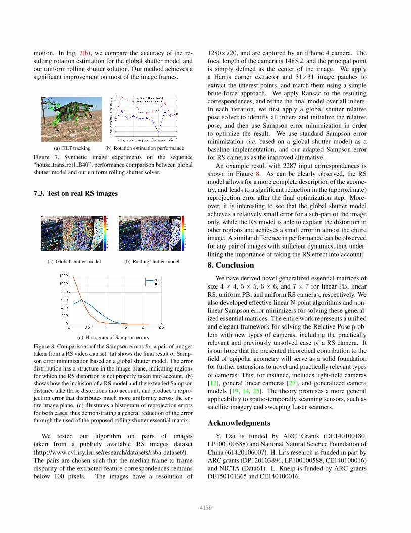
motion. In Fig. 7(b), we compare the accuracy of the re-

sulting rotation estimation for the global shutter model and

our uniform rolling shutter solution. Our method achieves a

significant improvement on most of the image frames.

(a) KLT tracking (b) Rotation estimation performance

Figure 7. Synthetic image experiments on the sequence

“house trans rot1 B40”, performance comparison between global

shutter model and our uniform rolling shutter solver.

7.3. Test on real RS images

(a) Global shutter model (b) Rolling shutter model

(c) Histogram of Sampson errors

Figure 8. Comparisons of the Sampson errors for a pair of images

taken from a RS video dataset. (a) shows the final result of Samp-

son error minimization based on a global shutter model. The error

distribution has a structure in the image plane, indicating regions

for which the RS distortion is not properly taken into account. (b)

shows how the inclusion of a RS model and the extended Sampson

distance take those distortions into account, and produce a repro-

jection error that distributes much more uniformly across the en-

tire image plane. (c) illustrates a histogram of reprojection errors

for both cases, thus demonstrating a general reduction of the error

through the used of the proposed rolling shutter essential matrix.

We tested our algorithm on pairs of images

taken from a publicly available RS images dataset

(http://www.cvl.isy.liu.se/research/datasets/rsba-dataset/).

The pairs are chosen such that the median frame-to-frame

disparity of the extracted feature correspondences remains

below 100 pixels. The images have a resolution of

1280×720, and are captured by an iPhone 4 camera. The

focal length of the camera is 1485.2, and the principal point

is simply defined as the center of the image. We apply

a Harris corner extractor and 31×31 image patches to

extract the interest points, and match them using a simple

brute-force approach. We apply Ransac to the resulting

correspondences, and refine the final model over all inliers.

In each iteration, we first apply a global shutter relative

pose solver to identify all inliers and initialize the relative

pose, and then use Sampson error minimization in order

to optimize the result. We use standard Sampson error

minimization (i.e. based on a global shutter model) as a

baseline implementation, and our adapted Sampson error

for RS cameras as the improved alternative.

An example result with 2287 input correspondences is

shown in Figure 8. As can be clearly observed, the RS

model allows for a more complete description of the geome-

try, and leads to a significant reduction in the (approximate)

reprojection error after the final optimization step. More-

over, it is interesting to see that the global shutter model

achieves a relatively small error for a sub-part of the image

only, while the RS model is able to explain the distortion in

other regions and achieves a small error in almost the entire

image. A similar difference in performance can be observed

for any pair of images with sufficient dynamics, thus under-

lining the importance of taking the RS effect into account.

8. Conclusion

We have derived novel generalized essential matrices of

size 4 × 4, 5 × 5, 6 × 6, and 7 × 7 for linear PB, linear

RS, uniform PB, and uniform RS cameras, respectively. We

also developed effective linear N-point algorithms and non-

linear Sampson error minimizers for solving these general-

ized essential matrices. The entire work represents a unified

and elegant framework for solving the Relative Pose prob-

lem with new types of cameras, including the practically

relevant and previously unsolved case of a RS camera. It

is our hope that the presented theoretical contribution to the

field of epipolar geometry will serve as a solid foundation

for further extensions to novel and practically relevant types

of cameras. This, for instance, includes light-field cameras

[12], general linear cameras [27], and generalized camera

models [19, 14, 25]. The theory promises a more general

applicability to spatio-temporally scanning sensors, such as

satellite imagery and sweeping Laser scanners.

Acknowledgments

Y. Dai is funded by ARC Grants (DE140100180,

LP100100588) and National Natural Science Foundation of

China (61420106007). H. Li’s research is funded in part by

ARC grants (DP120103896, LP100100588, CE140100016)

and NICTA (Data61). L. Kneip is funded by ARC grants

DE150101365 and CE140100016.

4139

References

[1] O. Ait-Aider, N. Andreff, J. Lavest, and P. Martinet. Simul-

taneous object pose and velocity computation using a sin-

gle view from a rolling shutter camera. In Proc. Eur. Conf.

Comp. Vis., pages 56–68. 2006. 2

[2] O. Ait-Aider and F. Berry. Structure and kinematics trian-

gulation with a rolling shutter stereo rig. In Proc. IEEE Int.

Conf. Comp. Vis., pages 1835–1840, Sept 2009. 2

[3] C. Albl, Z. Kukelova, and T. Pajdla. R6p - rolling shutter

absolute camera pose. In Proc. IEEE Conf. Comp. Vis. Patt.

Recogn., June 2015. 1, 2

[4] P.-E. Forssen and E. Ringaby. Rectifying rolling shutter

video from hand-held devices. In Proc. IEEE Conf. Comp.

Vis. Patt. Recogn., pages 507–514, June 2010. 7

[5] M. Grundmann, V. Kwatra, D. Castro, and I. Essa.

Calibration-free rolling shutter removal. In ICCP, pages 1–8,

April 2012. 2

[6] R. Gupta and R. Hartley. Linear pushbroom cameras. IEEE

Trans. Pattern Anal. Mach. Intell., 19(9):963–975, Sep 1997.

2, 5

[7] R. Hartley. In defense of the eight-point algorithm. IEEE

Trans. Pattern Anal. Mach. Intell., 19(6):580–593, Jun 1997.

6

[8] R. I. Hartley and A. Zisserman. Multiple View Geometry

in Computer Vision. Cambridge University Press, ISBN:

0521540518, second edition, 2004. 6

[9] J. Hedborg, P.-E. Forssen, M. Felsberg, and E. Ringaby.

Rolling shutter bundle adjustment. In Proc. IEEE Conf.

Comp. Vis. Patt. Recogn., pages 1434–1441, June 2012. 1, 2

[10] J. Hedborg, E. Ringaby, P.-E. Forssen, and M. Felsberg.

Structure and motion estimation from rolling shutter video.

In International Conference on Computer Vision Workshops,

pages 17–23, Nov 2011. 2

[11] S. Im, H. Ha, G. Choe, H.-G. Jeon, K. Joo, and I. S. Kweon.

High quality structure from small motion for rolling shut-

ter cameras. In Proc. IEEE Int. Conf. Comp. Vis., Santiago,

Chile, 2015. 1, 2

[12] O. Johannsen, A. Sulc, and B. Goldluecke. On linear struc-

ture from motion for light field cameras. In Proc. IEEE Int.

Conf. Comp. Vis., 2015. 8

[13] C. Kerl, J. Stueckler, and D. Cremers. Dense continuous-

time tracking and mapping with rolling shutter RGB-D cam-

eras. In Proc. IEEE Int. Conf. Comp. Vis., Santiago, Chile,

2015. 1, 2, 3

[14] H. Li, R. Hartley, and J.-H. Kim. A linear approach to motion

estimation using generalized camera models. In Proc. IEEE

Conf. Comp. Vis. Patt. Recogn., pages 1–8, June 2008. 8

[15] L. Magerand, A. Bartoli, O. Ait-Aider, and D. Pizarro.

Global optimization of object pose and motion from a sin-

gle rolling shutter image with automatic 2d-3d matching. In

Proc. Eur. Conf. Comp. Vis., pages 456–469, 2012. 1, 2

[16] M. Meingast, C. Geyer, and S. Sastry. Geometric models of

rolling-shutter cameras. In OMNIVIS, 2005. 2, 5

[17] L. Oth, P. Furgale, L. Kneip, and R. Siegwart. Rolling shutter

camera calibration. In Proc. IEEE Conf. Comp. Vis. Patt.

Recogn., pages 1360–1367, June 2013. 2

[18] A. Patron-Perez, S. Lovegrove, and G. Sibley. A spline-

based trajectory representation for sensor fusion and rolling

shutter cameras. Int. J. Comput. Vision, 113(3):208–219,

July 2015. 3

[19] R. Pless. Using many cameras as one. In Proc. IEEE Conf.

Comp. Vis. Patt. Recogn., pages 587–593, June 2003. 8

[20] J. Ponce. What is a camera? In Proc. IEEE Conf. Comp. Vis.

Patt. Recogn., pages 1526–1533, June 2009. 2

[21] O. Saurer, K. Koser, J.-Y. Bouguet, and M. Pollefeys. Rolling

shutter stereo. In Proc. IEEE Int. Conf. Comp. Vis., pages

465–472, Dec 2013. 1, 2

[22] O. Saurer, M. Pollefeys, and G. H. Lee. A minimal solution

to the rolling shutter pose estimation problem. In IEEE/RSJ

International Conference on Intelligent Robots and Systems,

2015. 1, 2

[23] Y. Sheikh, A. Gritai, and M. Shah. On the spacetime geome-

try of galilean cameras. In Proc. IEEE Conf. Comp. Vis. Patt.

Recogn., pages 1–8, June 2007. 5

[24] G. S. Steven Lovegrove, Alonso Patron-Perez. Spline fusion:

A continuous-time representation for visual-inertial fusion

with application to rolling shutter cameras. In Proc. Brit.

Mach. Vis. Conf., 2013. 3

[25] P. Sturm. Multi-view geometry for general camera models.

In Proc. IEEE Conf. Comp. Vis. Patt. Recogn., pages 206–

212, June 2005. 4, 5, 8

[26] F. Vasconcelos and J. Barreto. Towards a minimal solution

for the relative pose between axial cameras. In Proc. Brit.

Mach. Vis. Conf., 2013. 4

[27] J. Yu and L. McMillan. General linear cameras. In T. Pajdla

and J. Matas, editors, Proc. Eur. Conf. Comp. Vis., volume

3022 of Lecture Notes in Computer Science, pages 14–27.

Springer Berlin Heidelberg, 2004. 2, 8

4140