Rolling Shutter Bundle Adjustment

Johan Hedborg Per-Erik Forssen Michael Felsberg Erik Ringaby

Computer Vision Laboratory, Department of Electrical Engineering Linkoping University, Sweden

Abstract

This paper introduces a bundle adjustment (BA) method

that obtains accurate structure and motion from rolling

shutter (RS) video sequences: RSBA. When a classical BA

algorithm processes a rolling shutter video, the resultant

camera trajectory is brittle, and complete failures are not

uncommon. We exploit the temporal continuity of the cam-

era motion to define residuals of image point trajectories

with respect to the camera trajectory. We compare the cam-

era trajectories from RSBA to those from classical BA, and

from classical BA on rectified videos. The comparisons

are done on real video sequences from an iPhone 4, with

ground truth obtained from a global shutter camera, rigidly

mounted to the iPhone 4. Compared to classical BA, the

rolling shutter model requires just six extra parameters. It

also degrades the sparsity of the system Jacobian slightly,

but as we demonstrate, the increase in computation time is

moderate. Decisive advantages are that RSBA succeeds in

cases where competing methods diverge, and consistently

produces more accurate results.

1. Introduction

Structure from motion (SfM) is one of the success stories

in computer vision [11]. SfM is now routinely used to add

visual effects to video, e.g. in the movie industry, and it has

been successfully used to build 3D models from both photo

collections, and from video [24]. Another technology that

uses SfM as its back-end is augmented reality [16].

An overwhelming majority of image sensors sold today

are of CMOS type: nearly all mobile video recording de-

vices, and most compact cameras have them. In contrast to

the classical CCD sensors, which have global sensor read-

out, the image rows of CMOS sensors are read out in rapid

succession over a readout time of 10-60 msec [28]. In ad-

dition, modern video recording devices come without a me-

chanical shutter, and instead reset the sensor elements elec-

tronically. These two effects combined constitute what is

known as an electronic rolling shutter, and lead to a rolling

shutter (RS) camera model [10].

Most work on SfM is based on the global shutter camera

Figure 1. If classical structure from motion is applied to rolling

shutter video, the result is unpredictable, whereas RSBA is stable.

These results are from sequence #19.

model [29, 11]. When used on rolling shutter cameras these

algorithms become brittle, e.g. Liu et al. [18] demonstrate

several cases where the Voodoo tracker1 fails, and similarly

Hedborg et al. [12] demonstrate failure of the SBA package

of Lourakis and Agyros [19] under rolling shutter.

1.1. Related work

Bundle adjustment (BA) is a collective name for tech-

niques that refine an initial estimate of structure and camera

motion, by minimising the reprojection errors over all im-

ages [29]. It has been shown that it is possible to use BA

solvers even in real time applications to improve SfM es-

timation [16, 6]. Other works have studied techniques for

improving the robustness of BA [22]. Recent progress has

been made in terms of stability and speed, especially for

large scale problems where several thousands cameras and

millions of points are refined and BA can now be used to

solve even city scale problems [9, 1, 13].

Despite the prevalence of rolling shutter cameras, sys-

tems that model rolling shutter cameras are rare in the lit-

erature, and all previous work has modelled special cases.

In contrast, we present a system where the continuous

six degree-of-freedom camera trajectory is modelled under

rolling shutter geometry.

In an early study by Geyer et al. [10], rolling-shutter SfM

is estimated on synthetic data for fronto-parallel motions,

1http://www.digilab.uni-hannover.de/

1

��� �����������

����� ����������

�������

�����������

��

�������������

�� ��

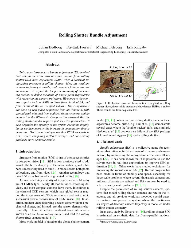
Figure 2. Flow-chart of the sequential SfM pipeline. Yellow boxes

were added/modified by [12]. In this paper, we skip the point recti-

fication step, and instead make rolling-shutter versions of the blue

boxes. In [2, 16], only the PnP box was modified, and special

requirements on the initialisation were required.

and with a linearised screw motion model. Ego-motion un-

der known structure and rolling shutter cameras is studied

in [3]. A related study considers structure and motion on a

stereo rig where one of the cameras has a rolling shutter [4].

Ait-Aider et al. [2] solved the perspective-n-point (PnP)

[7] problem for rolling-shutter cameras where the camera

pose, and linear camera motion is estimated across one

frame only. Another PnP solution is the PTAM port to

iPhone 3G by Klein et al. [16]. As both of these solutions

use 2D-3D correspondences, they require an initially known

3D structure. In the PTAM case the initial 3D structure is

found by requiring that the start of the sequence images a

planar scene. As the initial 3D structure is assumed to be

correct, the solution can easily deteriorate over time.

Another recent line of work is to first rectify the frames,

and then apply the classical global shutter SfM pipeline

[12]. While this has been demonstrated to work in several

cases, the accuracy of the reconstruction is critically depen-

dent on the initial rectification, and any model errors in the

rectification will also propagate to the final solution.

Figure 2 is an overview of the SfM pipeline. First an ini-

tial structure and motion estimate is found using techniques

described in section 4. This is first bundle-adjusted, and

then new views are added in sequential fashion as shown

in the cycle at the bottom of the flow-chart. The contribu-

tions of this paper consist in making rolling-shutter aware

versions of the blue boxes, in particular we present the first

rolling shutter bundle adjustment method.

2. Bundle Adjustment

With Bundle Adjustment we refer to the process of re-

fining the complete set of camera parameters and 3D point

positions such that the error between the observed image

points and the projection of the 3D points is minimised

(aka. the reprojection error). The most common approach

to estimate these parameters is to pose it as a non-linear least

squares problem and solve it with the Levenberg-Marquardt

algorithm [17].

The distance metric between the reprojected point and

the observed point can either be the L2 norm, or differen-

tiable functions thereof, e.g. based on the Cauchy error dis-

tribution [6]. In this paper we follow the example of [19, 13]

and use the L2 norm error, but this can easily be modified

to use another norm if needed.

2.1. Levenberg­Marquardt Algorithm

The Levenberg-Marquardt algorithm is an iterative

method for minimising the quadratic norm of a vector val-

ued residual function r(x)

minx

1/2 ||r(x)||2 . (1)

Each iteration, xk+1 = xk + ∆x, solves a linear problem,

based on the Taylor expansion of r in xk [21]. The update

∆x is determined from the (damped) normal equations

(JTJ + λ diag(JTJ))∆x = −JTr(xk) , (2)

where λ > 0 is a damping parameter, and J = J(xk) is the

Jacobian J = ∂(r1, r2, ...)∂(x1, x2, ...) evaluated at point xk. The term

JTJ is an approximation of the Hessian of r(x). In order

to make the system better conditioned, we also scale our

system with a Jacobi preconditioner, as described in [1, 13].

2.2. Solving the normal equations

The linear system (2) grows large even for moderate

problems with a few hundred cameras. We use calibrated

cameras, which means 6 parameters for each camera pose,

and use 3 parameters for each 3D point. E.g. 200 cameras

and 10K 3D points gives a 31K×31K matrix, which is not

feasible to solve on most PCs, mainly due to memory usage.

Fortunately the 3D points and the cameras can be seen

as independent from each other, leading to sparse Jacobian

and approximate Hessian matrices. This independence is

weaker in the case of a rolling shutter system as we will see

later. An efficient handling of the sparsity is the key to solve

(2) in an efficient way and this is what distinguishes a BA

solver from a generic numerical solver.

The sparsity is typically exploited by applying the Schur

complement trick [29], which in a sense is a normal block

Gaussian elimination. The parameter vector consists of

camera parameters, c, and 3D model points, m, according

to xT = [cT mT]. The Jacobian is split accordingly into

J = [Jc Jm] = [∂(r1, r2, ...)∂(c1, c2, ...)

∂(r1, r2, ...)∂(m1, m2, ...) ], resulting in the

approximate Hessian:[

JTc Jc JT

c Jm

JTmJc JT

mJm

]

+ λ diag

[

JTc Jc 00 JT

mJm

]

=

[

U W

WT V

]

.

(3)

The normal equations (2) now read[

U W

WT V

] [

∆c

∆m

]

= −

[

JTc

JTm

]

r . (4)

The camera parameter update can now be computed sepa-

rately by elimination(

U−WV−1WT)

∆c =(

WV−1JTm − JT

c

)

r . (5)

The method of choice for solving the linear system (5) is

a Cholesky factorization due to the symmetry of the coeffi-

cient matrix (which is the Schur complement). How to do

this efficiently will be described in section 3.3.

Once we have the camera update, the update for the 3D

points is obtained as:

∆m = −V−1(JTmr + WT∆c) . (6)

Note that V is 3× 3 block diagonal, and this step is thus

very inexpensive. There is also a second sparsity structure

in the Schur complement (due to points not being visible

in all cameras). This becomes relevant when dealing with

large problems as noted in [1, 6].

3. Rolling Shutter Bundle Adjustment

We present a Bundle Adjustment solver for rolling shut-

ter cameras. We have chosen to look at video sequences

because this case is more tightly coupled than the image

collection case. In single frame rolling shutter models, we

get six [16], or more [2] extra camera parameters per frame.

In our approach, we interpolate between camera poses for

the first row of each frame, and instead get a total of six

extra parameters for the entire sequence.

3.1. Camera Model

In a rolling shutter camera, image rows are captured at

different time instances in sequential order. In the general

case this leads to different cameras poses for each row. Try-

ing to solve for all of these would lead to a heavily under-

determined system due to too few measurements. This

problem can be handled by only estimating a subset of the

poses, and representing the remaining ones using interpola-

tion. Many interpolation schemes can be used here but the

general rule is that if we increase the complexity of the in-

terpolation, we also increase the camera dependencies and

thus reduce the sparsity of the system Jacobian.

The interpolation chosen here follows the one proposed

in [8], using SLERP interpolation for the rotation [27] and

linear interpolation for the translation. We place key rota-

tions Rj and translations tj at the first row of each frame j.

The rolling shutter camera model for row y in frame j reads

Cj(y) = RTj,j+1(y)[ I | − tj,j+1(y)] (7)

where Rj,j+1(y) is the SLERP interpolated rotation be-

tween Rj and Rj+1, and similarly tj,j+1(y) is the inter-

polated translation. The method works for any number of

key rotations and translations per frame but we have chosen

to use just one per frame. In practise, a six parameter key

pose vector cj is used to represent a key pose {Rj , tj}.

� �� �� �� �� �� �� �� � �� � �� � �

�

�

��

��

��

��

��

��

��

��

��

��

�� �� �� �� �� �� �� �� � �� � �� � �

�

�

��

��

��

��

��

��

��

��

��

��

�

�� �

�� �

a) Jacobian Global Shutter b) Jacobian Rolling Shutter

�� �� �� �� ��

�

��

��

��

��

��

��

��

��

��

�� �� �� �� �� ��

��

��

��

��

��

��

�

���

c) Hessian Global Shutter d) Hessian Rolling Shutter

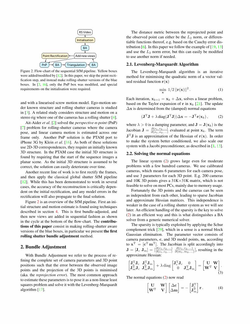
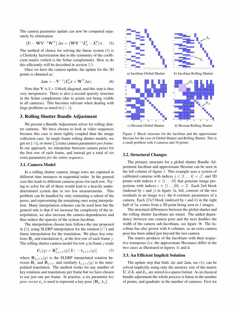
Figure 3. Block structure for the Jacobian and the approximate

Hessian for the case of Global Shutter and Rolling Shutter. This is

a small problem with 4 cameras and 10 points.

3.2. Structural Changes

The primary structure for a global shutter Bundle Ad-

justment Jacobian and approximate Hessian can be seen in

the left column of figure 3. This example uses a system of

calibrated cameras with indices j ∈ [1 . . . 4] = J , and 3D

points with indices k ∈ [1 . . . 10] that generate image pro-

jections with indices i ∈ [1 . . . 26] = I. Each 2x6 block

(indexed by i and j) in figure 3a, left, consists of the two

residuals in an image w.r.t. the 6 extrinsic parameters of a

camera. Each 2Ix3 block (indexed by i and k) in the right

half of 3a, comes from a 3D point being seen in I images.

The structural differences between the global shutter and

the rolling shutter Jacobians are minor. The added depen-

dency between one camera pose and the next doubles the

width of the camera sub-Jacobians, see figure 3b. The Ja-

cobian has also grown with 6 columns, as an extra camera

pose has been added just beyond the last camera.

The matrix products of the Jacobians with their respec-

tive transposes (i.e. the approximate Hessians) differ in the

two cases as illustrated in figures 3c and d.

3.3. An Efficient Implicit Solution

The update step that finds ∆c and ∆m, see (4), can be

solved implicitly using only the memory size of the matrix

U, if Jc and Jm are stored in a sparse format. As in classical

bundle adjustment the whole process is linear in the number

of points, and quadratic in the number of cameras. First we

solve for the camera update (5):

• Let Ik denote the index set of the image plane residuals

of 3D point mk (cf. figure 3b), and let Jk denote the

index set of the corresponding cameras Cj , j ∈ Jk.

Let Ji,j be the 2x12 sub-Jacobian that relates Cj and

the residual i = i(j, k) for the 3D point mk, as illus-

trated in figure 3b. The Jacobian Jc is formed by the

union of all Ji,j , for i ∈ I, j ∈ J .

• Compute U sequentially: First initialise U = 0, then,

for each 3D point mk do :

– For all cameras Cj , j ∈ Jk, U is updated ac-

cording to Uj,j ← Uj,j + JTi,jJi,j , where i =

i(j, k) and Uj,j is the 12x12 sub-matrix of U

corresponding to camera Cj , see figure 3d.

• To apply the regularization, we can now simply multi-

ply each diagonal element of U with 1 + λ.

• Compute b = −JTc r sequentially. First set b = 0,

then, for each 3D point mk do

– For all cameras Cj , j ∈ Jk and their corre-

sponding residuals ri, i = i(j, k), do bj ←bj − JT

i,jri, where bj is a 12x1 sub-matrix of

b, corresponding to Cj .

• Compute S = U − WV−1WT and b ← b +WV−1JT

mr. Initialize S = U. For each 3D point

mk do :

– Let Ji,k be the 2x3 sub-Jacobian for 3D point in-

dex k and image point index i ∈ Ik. The Jaco-

bian Jm is formed by the union of all Ji,k, for

i ∈ I, and j ∈ J .

– Construct the 3x3 matrix Vk,k =∑

i∈Ik

JTi,kJi,k.

– For all combinations of cameras (Cj1 ,Cj2),where j1, j2 ∈ Jk (accordingly i1 = i(j1, k)and i2 = i(j2, k)), update sub-matrices of S as

Sj1,j2 ← Sj1,j2−JTi1,j1

Ji1,kV−1k,kJ

Ti2,kJi2,j2 and

bj1 ← bj1 + JTi1,j1

Ji1,kV−1k,kJ

Ti2,kri2 .

• Finally, the update step for the cameras is completed

by solving the symmetric linear system S∆c = b.

The points update (6) is computationally of low com-

plexity and is implemented in the following way:

• For each 3D point mk do :

– Compute: ai = ri + Ji,j∆cj

for all i = i(j, k) ∈ Ik, (and thus j ∈ Jk).

– Compute the 3D point update as:

∆mk = −V−1k,k

∑

i∈Ik

JTi,kai , where

Further efficiency can be gained by using symmetry to

avoid repeating some computations twice. For instance, a

more efficient (but less readable) implementation can be

found by reordering the cameras, and using BLAS32 [13].

2BLAS3 is a library of matrix-matrix operations.

3.4. Jacobian Calculations

Each sub-Jacobian Ji,j contains the derivatives of ri

w.r.t. the camera key pose vectors cj and cj+1. It is

straight-forward to find the analytic expressions for the sub-

Jacobians Ji,j , and Ji,k using basic differential calculus on

r, but some details of the derivation are worth mentioning:

• We use unit quaternions q =(

cos θ2 , sin θ

2 n)

to com-

pute rotations, but parameterise the rotations using just

the last three elements of q.

• Each step of the processing chain is derived separately,

and steps are concatenated using the chain rule.

• In the rolling shutter case, however, each individual

residual has its own camera pose. This pose is a func-

tion of both the two nearest key poses, and of the ob-

served image point.

4. Structure from Motion

The proposed bundle adjustment method is an essential

part of the structure from motion (SfM) estimation pipeline

shown in figure 2. In this section we provide details on how

the other components of SfM are implemented in both the

global shutter and the rolling shutter cases.

4.1. Point correspondences

All components in the SfM pipeline use inter-frame cor-

respondences as measurements. These are found by first de-

tecting interest points in each frame, using the FAST detec-

tor [26], and then tracking these with the KLT-tracker [20].

New points detected near existing trajectories are discarded

in order to have the number of points fairly constant.

A first outlier rejection is done using cross-checking [5].

First points are tracked forward in time, and then the track-

ing is reversed. Only points that return to their original posi-

tions (within a threshold) are kept. This effectively removes

most outliers from the tracker, without having to resort to

global-shutter constraints such as homographies or funda-

mental/essential matrices. This is important, as these con-

straints are not satisfied under rolling-shutter geometry.

4.2. Global Shutter Structure from Motion

Here we describe the version of global shutter structure

from motion, which we compare with rolling shutter SfM in

the experiments. The description follows figure 2.

First, we build an initial geometry from three views with

a sufficient relative baseline, using the five point method

[23]. The essential matrices (and relative poses) between

three views are robustly estimated in a RANSAC loop, and

the 3D points are triangulated using the optimal method

from [14]. The intermediate views are then added, and ev-

erything is bundled.

New views are successively added using the standard,

sequential approach shown in figure 2. Here four views

are added at a time (this can be considered restrictive, as

we are restricted to video input). First a PnP is applied,

which minimises the L2 error between the reprojected 3D

model points, and the tracked points in the new frame that

survived cross-checking (see section 4.1). This direct ap-

proach works well, as we can trust the 3D model points to

be accurate. This is also exploited in PTAM [16].

Before new point tracks are added, a second level of out-

lier rejection is applied, using the scale-normalised standard

deviation of multiple triangulations

σX =1

||tw − µX||

√

1M−1

∑Mm=1(Xm − µ

X)2 . (8)

The points Xm are triangulations between the first camera

in a track, and all subsequent cameras where it is present,

and µX

is their mean. tw is our frame of reference, cho-

sen as the camera with the middle index in this sequence.

Tracks where σX is above a threshold, are discarded.

Bundle adjustment (BA), as described in section 2 is ap-

plied, after the initial geometry has been estimated, as well

as after all PnP and Triangulation steps. Running BA after

PnP is especially important, as the outlier rejection step (8)

relies on accurate poses.

4.3. Rolling Shutter Structure from Motion

Just like in the global shutter case, the rolling shutter

aware SfM requires an initial estimate of structure and mo-

tion. For this we make use of the method suggested in [12],

where the tracked points are first rectified using a 3D rota-

tion model. This pre-rectification of points allows us to use

global shutter geometric constraints, and consequently we

then use the same initialisation as in the global shutter case,

see section 4.2.

The original distorted points are however saved and sub-

sequently used in the rolling shutter bundle adjustment, as

described in section 3. The rolling shutter SfM follows the

same scheme as the global shutter SfM (described in 4.2),

but instead of using global shutter PnP, triangulation and

bundle adjustment we use rolling shutter versions of these

methods, as indicated in figure 2.

4.4. Rolling Shutter PnP and Triangulation

Ait-Aider et al. [2] solved the rolling shutter PnP prob-

lem by estimating the camera pose and linear camera mo-

tion during one frame. We instead propose to jointly esti-

mate all the new poses. This allows us to exploit the cou-

pling between poses, and thus constrain the problem better.

The minimisation is done over the L2 reprojection error be-

tween 3D points and tracked image points as with the global

shutter PnP. Again, we use the RS camera model (7), with

linear interpolation between camera positions, and SLERP

interpolated rotations. This multi-frame PnP can be posed

as the following optimisation problem:

mincN ,..,cN+L

1

2

N+L−1∑

j=N

∑

k∈Vj

dist(pj,k,Cj(y)Xk)2 . (9)

Here N is index for the first of the new poses, L is the num-

ber of new views, and Vj is the index set of visible points

in camera j, thus Xk, k ∈ Vj is a 3D point, which is visible

in camera j. Further, pj,k is the observation of 3D point kin camera j and Cj(y) = C(cj , cj+1, y) is an interpolated

camera defined as in (7). Finally, dist(·, ·) is the Euclidean

distance in image the plane.

We use the Levenberg-Marquardt algorithm, initialized

with the previous camera, to solve (9). Note that an extra

pose is estimated, cN+L. This pose does not have the same

support as the rest of the parameters, and we currently dis-

card it after estimation.

The rolling shutter aware triangulation method is similar

to the classical optimal triangulation [14]. The only differ-

ence is that the two camera matrices are now a function of

the current image row, see (7).

5. Experiments

In this section we describe our experimental setup for

comparison of bundle adjustment methods on rolling shutter

cameras. The evaluation is done by comparing the obtained

camera trajectories to a reference trajectory.

5.1. Experiment Setup

All experiments use video from an iPhone 4 camera

recorded at 1280 × 720 resolution, at 30 fps. Our evalu-

ation is based on accurate reference trajectories, obtained

using a second camera that has a global shutter, a Canon

S95 with 1280 × 720 resolution, at 24 fps. This prosumer

compact camera produces good image quality due to a rela-

tively large image sensor (1/1.7”). This combined with the

wide angle lens allows very accurate camera trajectory es-

timation. The reprojection error is around 0.2 pixel which

is around a third of the error for the rolling shutter SfM on

the iPhone data. For the iPhone 4 readout time, we use the

value of 32.37 msec, as listed in [25].

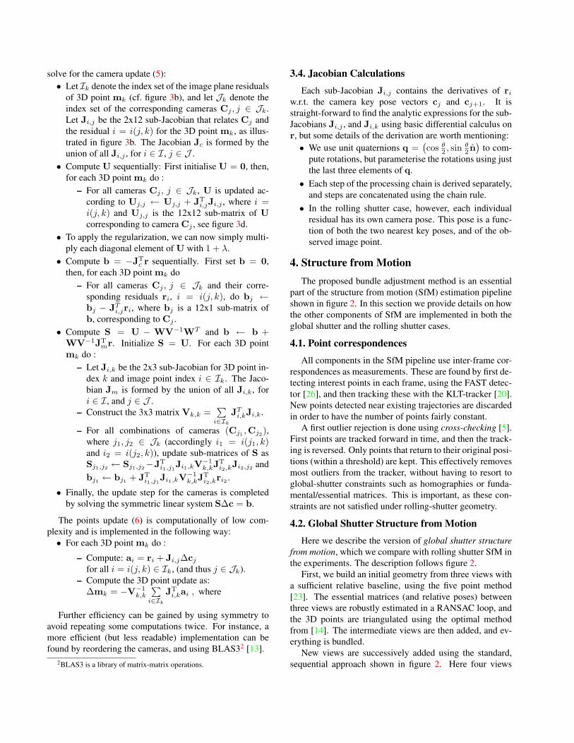
The two cameras are rigidly mounted on a rig, with over-

lapping fields of view, and optical centers as close as pos-

sible, see figure 4. Both cameras are calibrated for intrin-

sic camera parameters, radial, and tangential distorsions, al-

lowing us to use calibrated epipolar geometry throughout.

For frame-accurate synchronization, we start and end

each recording with a snap of fingers, which is visible in

both cameras. The maximal error in this synchronization is

a function of the lower of the two frame rates. Here we get

1/24 sec as maximal error, which is small compared to the

length of our sequences (typically around 4 seconds).

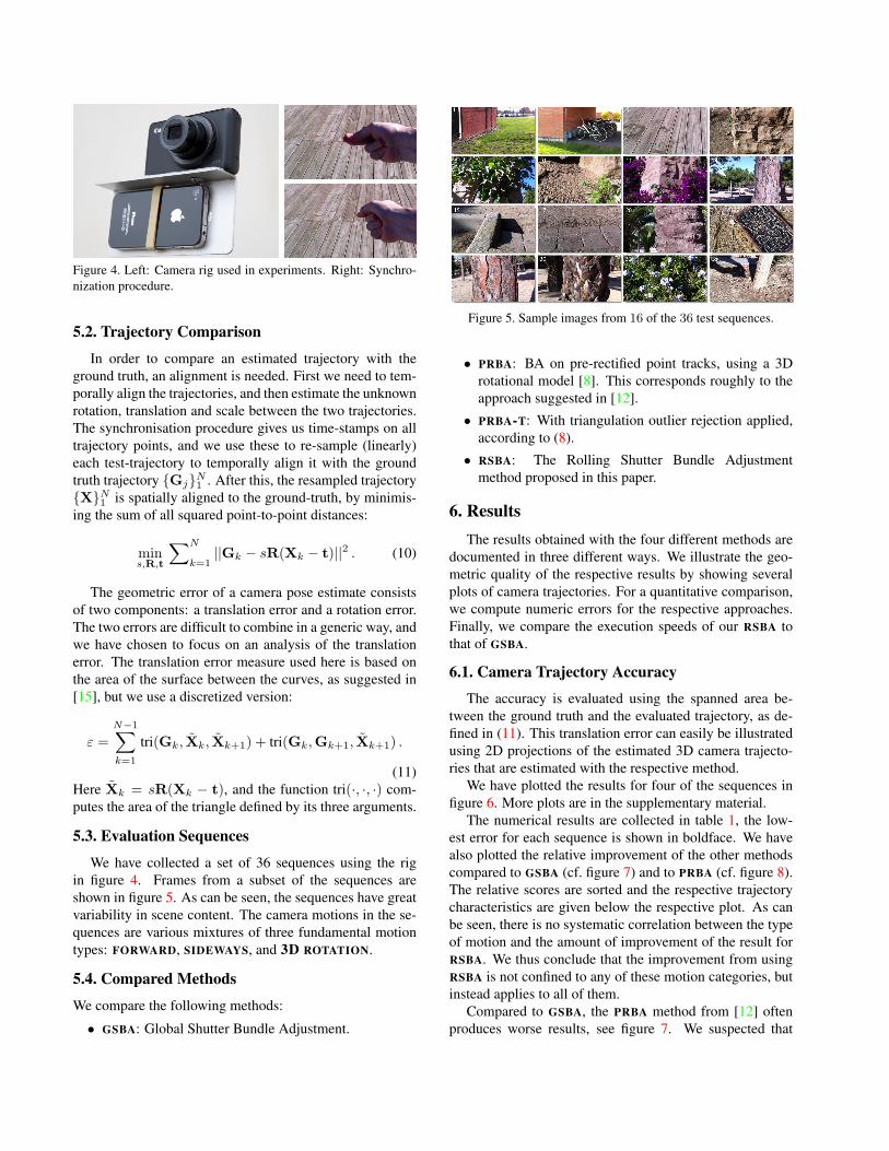
Figure 4. Left: Camera rig used in experiments. Right: Synchro-

nization procedure.

5.2. Trajectory Comparison

In order to compare an estimated trajectory with the

ground truth, an alignment is needed. First we need to tem-

porally align the trajectories, and then estimate the unknown

rotation, translation and scale between the two trajectories.

The synchronisation procedure gives us time-stamps on all

trajectory points, and we use these to re-sample (linearly)

each test-trajectory to temporally align it with the ground

truth trajectory {Gj}N1 . After this, the resampled trajectory

{X}N1 is spatially aligned to the ground-truth, by minimis-

ing the sum of all squared point-to-point distances:

mins,R,t

∑N

k=1||Gk − sR(Xk − t)||2 . (10)

The geometric error of a camera pose estimate consists

of two components: a translation error and a rotation error.

The two errors are difficult to combine in a generic way, and

we have chosen to focus on an analysis of the translation

error. The translation error measure used here is based on

the area of the surface between the curves, as suggested in

[15], but we use a discretized version:

ε =

N−1∑

k=1

tri(Gk, Xk, Xk+1) + tri(Gk,Gk+1, Xk+1) .

(11)

Here Xk = sR(Xk − t), and the function tri(·, ·, ·) com-

putes the area of the triangle defined by its three arguments.

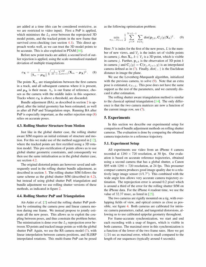
5.3. Evaluation Sequences

We have collected a set of 36 sequences using the rig

in figure 4. Frames from a subset of the sequences are

shown in figure 5. As can be seen, the sequences have great

variability in scene content. The camera motions in the se-

quences are various mixtures of three fundamental motion

types: FORWARD, SIDEWAYS, and 3D ROTATION.

5.4. Compared Methods

We compare the following methods:

• GSBA: Global Shutter Bundle Adjustment.

Figure 5. Sample images from 16 of the 36 test sequences.

• PRBA: BA on pre-rectified point tracks, using a 3D

rotational model [8]. This corresponds roughly to the

approach suggested in [12].

• PRBA-T: With triangulation outlier rejection applied,

according to (8).

• RSBA: The Rolling Shutter Bundle Adjustment

method proposed in this paper.

6. Results

The results obtained with the four different methods are

documented in three different ways. We illustrate the geo-

metric quality of the respective results by showing several

plots of camera trajectories. For a quantitative comparison,

we compute numeric errors for the respective approaches.

Finally, we compare the execution speeds of our RSBA to

that of GSBA.

6.1. Camera Trajectory Accuracy

The accuracy is evaluated using the spanned area be-

tween the ground truth and the evaluated trajectory, as de-

fined in (11). This translation error can easily be illustrated

using 2D projections of the estimated 3D camera trajecto-

ries that are estimated with the respective method.

We have plotted the results for four of the sequences in

figure 6. More plots are in the supplementary material.

The numerical results are collected in table 1, the low-

est error for each sequence is shown in boldface. We have

also plotted the relative improvement of the other methods

compared to GSBA (cf. figure 7) and to PRBA (cf. figure 8).

The relative scores are sorted and the respective trajectory

characteristics are given below the respective plot. As can

be seen, there is no systematic correlation between the type

of motion and the amount of improvement of the result for

RSBA. We thus conclude that the improvement from using

RSBA is not confined to any of these motion categories, but

instead applies to all of them.

Compared to GSBA, the PRBA method from [12] often

produces worse results, see figure 7. We suspected that

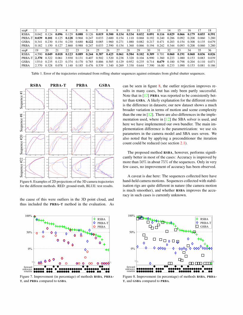
seq# 1 2 3 4 5 6 7 8 9 10 11 12 13 14 15 16 17 18

RSBA 0.042 0.124 0.096 0.129 0.088 0.126 0.019 0.500 0.154 0.534 0.032 0.091 0.116 0.029 0.066 0.179 0.055 0.591

PRBA-T 0.039 0.101 0.125 0.128 0.968 0.247 0.033 2.600 0.154 1.110 0.068 0.192 0.240 0.286 0.092 0.208 0.060 3.280

GSBA 0.341 0.230 0.154 0.230 0.680 0.122 0.085 1.960 0.271 1.080 0.082 0.217 0.471 0.203 0.154 0.308 0.135 0.679

PRBA 0.182 1.150 0.127 2.860 0.988 0.247 0.033 2.590 0.154 1.360 0.066 0.194 0.242 0.344 0.093 0.208 0.060 3.280

seq# 19 20 21 22 23 24 25 26 27 28 29 30 31 32 33 34 35 36

RSBA 4.590 0.049 0.018 0.123 0.089 0.244 0.387 0.425 0.061 0.584 0.102 0.309 0.701 0.060 0.191 0.068 0.036 0.026

PRBA-T 2.370 0.322 0.061 3.930 0.131 0.407 0.502 1.520 0.238 3.320 0.104 6.990 1.360 0.233 1.080 0.153 0.083 0.039

GSBA 135.0 0.235 0.123 0.374 0.170 0.785 0.886 0.585 0.129 0.952 0.235 0.714 0.679 0.180 0.798 0.204 0.110 0.071

PRBA 2.370 0.328 0.078 1.140 0.185 0.476 0.539 1.340 0.269 3.330 0.644 7.390 16.00 0.233 1.090 0.153 0.081 0.186

Table 1. Error of the trajectories estimated from rolling shutter sequences against estimates from global shutter sequences.

RSBA PRBA-T PRBA GSBA

Seq

uen

ce#

1

−6 −4 −2

20

30

40

50

60

70

−6 −4 −2

20

30

40

50

60

70

−6 −4 −2

20

30

40

50

60

70

−6 −4 −2

20

30

40

50

60

70

Seq

uen

ce#

8

0 10 20

0

10

20

30

40

50

60

0 10 20

0

10

20

30

40

50

60

0 10 20

0

10

20

30

40

50

60

0 10 20

0

10

20

30

40

50

60

Seq

uen

ce#

20

−10 −5 0

−2.5

−2

−1.5

−1

−0.5

0

0.5

−10 −5 0

−2.5

−2

−1.5

−1

−0.5

0

0.5

−10 −5 0

−2.5

−2

−1.5

−1

−0.5

0

0.5

−10 −5 0

−2.5

−2

−1.5

−1

−0.5

0

0.5

Seq

uen

ce#

22

−4 −2 0

0

5

10

15

20

25

30

−4 −2 0

0

5

10

15

20

25

30

−4 −2 0

0

5

10

15

20

25

30

−4 −2 0

0

5

10

15

20

25

30

Figure 6. Examples of 2D projections of the 3D camera trajectories

for the different methods. RED: ground-truth, BLUE: test results.

the cause of this were outliers in the 3D point cloud, and

thus included the PRBA-T method in the evaluation. As

��

���

����

�������� �����������

����

������

����

Figure 7. Improvement (in percentage) of methods RSBA, PRBA-

T, and PRBA compared to GSBA.

can be seen in figure 8, the outlier rejection improves re-

sults in many cases, but has only been partly successful.

Note that in [12] PRBA was reported to be consistently bet-

ter than GSBA. A likely explanation for the different results

is the difference in datasets; our new dataset shows a much

broader variation in terms of motion and scene complexity

than the one in [12]. There are also differences in the imple-

mentation used, where in [12] the SBA solver is used, and

here we have implemented our own bundler. The main im-

plementation difference is the parametrization: we use six

parameters in the camera model and SBA uses seven. We

also noted that by applying a preconditioner the iteration

count could be reduced (see section 2.1).

The proposed method RSBA, however, performs signifi-

cantly better in most of the cases: Accuracy is improved by

more than 50% in about 75% of the sequences. Only in very

few cases, no improvement of accuracy has been observed.

A caveat is due here: The sequences collected here have

hand-held camera motions. Sequences collected with stabil-

isation rigs are quite different in nature (the camera motion

is much smoother), and whether RSBA improves the accu-

racy in such cases is currently unknown.

��

���

����

�������� �����������

����

������

����

Figure 8. Improvement (in percentage) of methods RSBA, PRBA-

T, and GSBA compared to PRBA.

6.2. Computational Speed

Our GSBA run on a sequence with 221 cameras com-

puted 13 777 structure points in 5 iterations. This took on

average 4.91 sec on a W3520 Intel PC. Our RSBA run on

the same sequence computed 14 320 structure points in 4iterations, and 8.37 sec, on average. On a smaller system

with 74 cameras, RSBA took 2.36 sec for 5 602 points,

while GSBA took 1.49 sec for 5 577 points. We have also

made preliminary comparisons with SBA [19]. On many

sequences our GSBA solver has similar complexity, but on

difficult sequences (e.g. with rolling shutter), our use of a

preconditioner leads to faster convergence.

7. Conclusions

In this paper, we have presented the RSBA, to the best

of our knowledge the first bundle adjustment system that

explicitly models rolling shutter geometry. Compared to

global shutter BA, the increase in computation time is mod-

erate. Using real image sequences captured with an iPhone

4, we have demonstrated that our proposed method consis-

tently improves the accuracy of SfM across a wide variety

of camera motions. This is a first attempt at rolling shut-

ter bundle adjustment, and there are many things that can

be improved. In the future we plan to investigate other tra-

jectory representations, and other cost functions that are not

based on the L2 norm.

Acknowledgements This work has been supported by ELLIIT,

the Strategic Area for ICT research, funded by the Swedish

Government, and from VPS, funded by the Swedish Foundation

for Strategic Research. The CENIIT organisation at LiTH, the

Swedish Research Council through a grant for the project Embod-

ied Visual Object Recognition, and by Linkoping University.

References

[1] S. Agarwal, N. Snavely, S. M. Seitz, and R. Szeliski. Bundle

adjustment in the large. In ECCV’10. 1, 2, 3

[2] O. Ait-Aider, N. Andreff, J. M. Lavest, and P. Martinet. Si-

multaneous object pose and velocity computation using a

single view from a rolling shutter camera. In ECCV’06, May

2006. 2, 3, 5

[3] O. Ait-Aider, A. Bartoli, and N. Andreff. Kinematics from

lines in a single rolling shutter image. In CVPR’07, Min-

neapolis, USA, June 2007. 2

[4] O. Ait-Aider and F. Berry. Structure and kinematics triangu-

lation with a rolling shutter stereo rig. In ICCV, 2009. 2

[5] S. Baker, D. Scharstein, J. P. Lewis, S. Roth, M. J. Black,

and R. Szeliski. A database and evaluation methodology for

optical flow. In IEEE ICCV, Rio de Janeiro, Brazil, 2007. 4

[6] C. Engels, H. Stewenius, and D. Nister. Bundle adjustment

rules. In Photogrammetric Computer Vision, 2006. 1, 2, 3

[7] M. A. Fischler and R. C. Bolles. Random sample consen-

sus: A paradigm for model fitting with applications to im-

age analysis and automated cartography. Commun. ACM,

24:381–395, June 1981. 2

[8] P.-E. Forssen and E. Ringaby. Rectifying rolling shutter

video from hand-held devices. In CVPR’10. 3, 6

[9] J.-M. Frahm, P. Georgel, D. Gallup, T. Johnson, R. Ragu-

ram, C. Wu, Y.-H. Jen, E. Dunn, B. Clipp, S. Lazebnik,

and M. Pollefeys. Building rome on a cloudless day. In

ECCV’10, 2010. 1

[10] C. Geyer, M. Meingast, and S. Sastry. Geometric models of

rolling-shutter cameras. In 6th OmniVis WS, 2005. 1

[11] R. I. Hartley and A. Zisserman. Multiple View Geometry in

Computer Vision. Cambridge University Press, 2004. 1

[12] J. Hedborg, E. Ringaby, P.-E. Forssen, and M. Felsberg.

Structure and motion estimation from rolling shutter video.

In IWMV workshop at ICCV’11, 2011. 1, 2, 5, 6, 7

[13] Y. Jeong, D. Nister, D. Steedly, R. Szeliski, and I.-S. Kweon.

Pushing the envelope of modern methods for bundle adjust-

ment. In CVPR’10, June 2010. 1, 2, 4

[14] K. Kanatani, Y. Sugaya, and H. Niitsuma. Triangulation

from two views revisited: Hartley-sturm vs. optimal correc-

tion. In BMVC, pages 173–182, 2008. 4, 5

[15] K. Kishimoto. On a distance between two curves. In First

Int. Symp. for Science on Form, pages 121–128, 1986. 6

[16] G. Klein and D. Murray. Parallel tracking and mapping on a

camera phone. In ISMAR’09, October 2009. 1, 2, 3, 5

[17] K. Levenberg. A method for the solution of certain non-

linear problems in least squares. Quarterly Journal of Ap-

plied Mathmatics, II(2):164–168, 1944. 2

[18] F. Liu, M. Gleicher, J. Wang, H. Jin, and A. Agarwala. Sub-

space video stabilization. ACM ToG, 30(1), 2011. 1

[19] M. A. Lourakis and A. Argyros. SBA: A Software Package

for Generic Sparse Bundle Adjustment. ACM Trans. Math.

Software, 36(1):1–30, 2009. 1, 2, 8

[20] B. Lucas and T. Kanade. An iterative image registration tech-

nique with an application to stereo vision. In IJCAI’81, pages

674–679, 1981. 4

[21] K. Madsen, H. B. Nielsen, and O. Tingleff. Methods for

non-linear least squares problems, 2nd ed. Technical report,

Technical University of Denmark, April 2004. 2

[22] D. Martinec and T. Pajdla. Robust rotation and translation

estimation in multiview reconstruction. In CVPR’07. 1

[23] D. Nister. An efficient solution to the five-point relative pose

problem. IEEE TPAMI, 6(26):756–770, June 2004. 4

[24] M. Pollefeys, L. van Gool, M. Vergauwen, F. Verbiest,

K. Cornelis, J. Tops, and R. Koch. Visual modeling with

a hand-held camera. IJCV, 59(3):207–232, 2004. 1

[25] E. Ringaby and P.-E. Forssen. Efficient video rectification

and stabilisation for cell-phones. IJCV, Online June 2011. 5

[26] E. Rosten and T. Drummond. Machine learning for high-

speed corner detection. In ECCV’06, May 2006. 4

[27] K. Shoemake. Animating rotation with quaternion curves. In

Int. Conf. on CGIT, pages 245–254, 1985. 3

[28] G. Thalin. Camera rolling shutter amounts. http://www.

guthspot.se/video/deshaker.htm. 1

[29] B. Triggs, P. Mclauchlan, R. Hartley, and A. Fitzgibbon.

Bundle adjustment – a modern synthesis. In Vision Algo-

rithms: Theory and Practice, pages 298–375, 2000. 1, 2