FINAL REPORT
RL-34 RING LASER GYRO
LABORATORY EVALUATION
FOR THE
DEEP SPACE NETWORK
ANTENNA APPLICATION
JPL CONTRACT NO. 959072
28 NOVEMBER 1991
This report was prepared for the Jet Propulsion Laboratory,California Institute of Technology, sponsored by the
National Aeronautics and Space Administration.
Allied-Signal Aerospace Company _IsiliedgnalBendixGuidanceSystemsOivision
https://ntrs.nasa.gov/search.jsp?R=19920022884 2018-09-09T12:17:12+00:00Z

Table of Contents
I. Introduction
Definition of coordinates
II. Test Plans
III. Facility & Metrology Description
IV. RLG Array Description, and test configurations
V. Data acquisition and processing description
VI. Processed test data summary records
Initialization
Blind Acquisition Testing
Target Tracking Tests
VII. Parametric error model
VIII. Error allocation and overall system performance
IX. Recommended alternatives to improve performance
X Summary
Appendix A:
Appendix B:
Appendix C:
Appendix D:
Appendix E:
Appendix F:
Copy of letter sent to Noble Nerheim withinitial raw data records
Explanation of Navigation Equations
Tracking Data
Gyro Data over Temperature and Thermal
Model
Differential Equation Gyro Model
Description of Raw Data Records
7
8
15
22
23
32
45
59
60
62
63
List of FigurgsFigure 1
Figure 2
Figure 3
Figure 4
Figure 5
Figure 6
Figure 7
Figure 8
Figure 9
Figure 10
Figure 11
Figure 12
Figure 13
Figure 14
Figure 15
Figure 16
Figure 17
Figure 18
Figure 19
Figure 20
Figure 21
Figure 22
Figure 23
Figure 24
Figure 25
RL-34 High Accuracy RLG
RL-34 ISA Assembly
Definition of System's Roll, Pitch, and Heading
System Readout in Mils and Degs
Three Axis Dividing Head Test Site
Air Bearing Test Site
Theodolite Setup
Theodolite Setup with porto prism
Sigma Plot with Graphical Curve Fit
Sigma Plot with Computer Curve FitAzimuth Error Due to Boresite Errors
Elevation Error Due to Boresite Errors
Blind Target Acquisition Test Results at 0.5 dps
Blind Target Acquisition Test Results at 0.2 dps
System Temperature Warm Up
Tracking Test (typical)
Tracking Test (best)
Overlay of Azimuth Tracking Errors for 1st 6 tests
Azimuth Tracking Errors post Recalibration
Azimuth Tracking Errors at 60 deg Elevation
RMS Pointing Error vs Time for Runs 1-6
RMS Pointing Error vs Time for Runs 7-12
RMS Pointing Error vs Time for Runs 7-8
RMS Pointing Error vs Time for Runs 1-12
X32 Reduced Quantization Allan Variance Plot
2
3
5
6
9
10
12
13
18
19
37
37
39
40
44
47
48
5O
51
53
55
56
57
58
61
ii

List of Table_Table I
Table II
Table IIITable IV
Table V
Table VI
Table VII
Table VIII
Table IX
Table X
Table XI
Table XII
Table XIII
Table XIV
Table XV
Example of Calculations for a Sigma Plot 17
Calibration Data at four positions 23
List of Azimuth at Completion of Alignment 24
Summary of Gyro Compass Accuracy at 8 Positions 25
Summary of Additional Gyro Compass Positions 26Azimuth Error Corrected for Bias Errors 28
Summary of Repeated Alignment Tests 29
Initialization Error Based on Gyro Noise Model 30Azimuth Error vs Rotation Rate 33
Typical Compound Angle Acquisition Test 36
Summary of Blind Target Acquisition 41
Temperature Warm Up 43
Z Gyro Bias Changes during Acquisition software
Changes 45
Calibration data before second set of trackingTests 46
Summary of Tracking Tests 49
°°°
111
I. Introduction
The Bendix designed RL-34 high accuracy ring laser gyro is the
basis of the testing done under this gyro evaluation contract (see
Figure 1). Three of these gyros were incorporated into an Inertial
Sensor Assembly(ISA) with three Sundstrand QA 2000
accelerometers. This ISA was installed into one of our Advanced
Land Navigation Systems which was then tested for pointing
accuracy (see Figure 2). The overall system pointing results agree
very well with the measured individual gyro performance, such that
pointing accuracy of a few millidegrees is feasible.
Pointing Performance vs. Objectives
Initialization
The initialization goal was to demonstrate the angular rate
error of an individual RLG to be less than 0.0002 deg/hr, rms, in the
determination of the Earth's spin vector. This translates to an
initialization pointing error of 0.001 degrees (3.7 arc-seconds) at the
BGSD latitude of 40.86 degrees. The final initialization pointing
results were 0.00086 degrees (3.1 arc-seconds), one sigma, thus
meeting the goal. These results encompassed 9 positions in the level
plane (azimuth), spanning the entire 360 degree range.
Blind Target Acquisition
The objective for the target acquisition mode was 0.0001
degrees (0.36 arc-seconds) individual RLG pointing error, after a 20
degree rotation at 0.1 degrees per second. Final tracking results
were limited by the digital quantization of the gyro output to 0.77
arc-seconds. An existing BGSD system electronics modification will
bring this value down to 0.18 arc-seconds, as explained in the
recommendations section later.
Target Tracking
The angular position error objective for target tracking was
0.001 degrees, rms, with a zero input rate for a period of I0 hours.
The best recorded test was 0.00136 degrees (4.9 arc-seconds) rms,for 10 hours. This was one of two tests that we believe were
representative of performance capabilities with proper calibration.
Together, they had a mean of 0.0022 degrees, rms.
The overall average tracking performance was 0.0038 degrees
(13.8 arc-seconds, all 12 tests). It should be noted that most of this
error occurs in azimuth, with average elevation error being less than
0.001 degrees. This difference is due to the strapdown system

2

Figure 2 RL-34 ISA Assembly

implementation, which is further explained in the body of the report,and in Appendix B.
Definition of System Roll, Pitch, and Heading
The standard nomenclature of a navigation system is defined in
terms of roll, pitch and heading. Figure 3 shows roll, pitch and
heading with respect to a North, East, and Up coordinate system.
Pitch is defined as the angle between the X system axis and the local
level plane. Heading is defined as the angle between North and the
projection of the X system axis onto the local level plane. Roll is the
angle of rotation around the X system axis. For the JPL/DSN
application, the two degrees of freedom for the antenna are azimuth
and elevation. They are related to the navigation system's heading
and pitch outputs, respectively. Throughout this report, heading and
azimuth will both be used, with azimuth being preferred. The same
is true for pitch and elevation, with elevation preferred. The
navigation system outputs all the angles in "mils" with 6400 mils in
360 degs. Figure 4 shows this convention applied to azimuth. North
corresponds to 0/6400 mils and East is 1600 mils. Most of the
analyzed data presented in this report has been converted to arc-sec
where 0.001 deg equal 3.6 arc-sec.
4

Q.
°_
X
X
0
Ih..
0
Z
%
"4'--#
ill
°,p-q
C.,
0
E
°m-d
o
o

North
0 mils
5600 mils800 mils
West
4800 milsEast
1600 mils
4000 mils2400 mils
South
3200 mils
The relationship between the system azimuth readout in Mils and Degrees.
Figure 4 System Readout in Mils and Degs
6

II. Test Plans
According to the statement of work, the test plan was
separated into three different areas: initialization, acquisition, and
tracking. We also realized the need for a more accurate gyro bias
calibration procedure and developed one accordingly. Please note
that the pointing accuracy objectives are such that gyro biases be
known to 0.0001 deg/hr. Our existing automated production
calibration techniques were designed to calibrate to 0.001 deg/hr,
which is required for high accuracy RLG based navigators.
Calibration Tests
To fine calibrate the gyro biases, a four position gyrocompass
test was performed (North, South, East, West). Each position required
6-8 hours of testing to average the random noise errors down to the
gyro bias stability limit (see appendix A on gyro data). The new
gyro biases were then changed and stored in the system for use in
future tests.
Initialization Tests
Once calibrated, the system gyrocompassed to determine its
attitude (see appendix B for system implementation). Since the
longest gyrocompass time allowed (production software limitation)
was 15 minutes, multiple gyro compasses were performed for 4-8 hr
test times. The qualification of the gyrocompass accuracy was
accomplished by testing 8 azimuth positions at 45 deg intervals.
Acquisition Tests
Once the system was initialized, the acquisition capability was
tested by rotating the system azimuth and elevation to acquire a
target. The rate table was used to rotate at various rates. The
elevation was changed with the Ultradex. The length of each test
was limited by the 100 second data update rate for the high rotation
rate tests or by the longer time of the low rotation rate test. Each
test was performed multiple times to generate performance and teststatistics.
Tracking Tests
All the tracking tests involved a 10 hour static navigation test.
Eight were performed at 0 deg elevation and 4 were performed at 60
deg elevation.
7

III, Test Facility and Metrology Descrintion
Bendix Facility
The geodetic latitude of Bendix's Teterboro complex is 40.86056
degrees. Within the facility, there are four outdoor geodetic survey
monuments to identify our geophysical location so we can cross
check each monument for accuracy. The monuments are calibrated
every 10 years by using a telescope-theodolite referring to the
"North Star" -- Polaris. The most recent calibration was done in
October, 1991. The overall accuracy to true north is within 2 arc-sec.
Using this as a primary north reference, "North" is transferred and
aligned to an indoor monument for all of our test measurements The
indoor "North" reference is located in our temperature controlled
system test area. The room temperature is controlled around 70 +/-5
deg F all year long.
For the purposes of this evaluation, two test sites were utilized.
The primary site was a Contraves rate table model 51C, with an air-
bearing table. On top of this table was mounted an Ultradex table.
Due to the time limitations of this contract, early results were
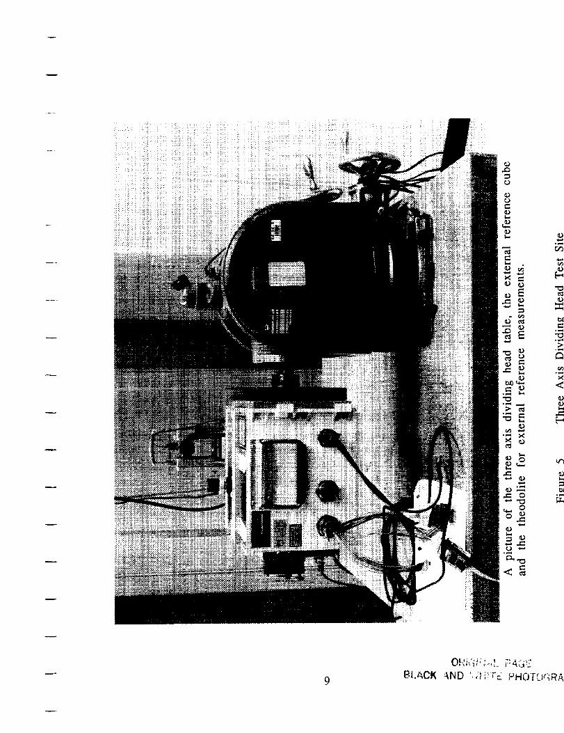
obtained on a three axis dividing head which was quickly set up
while the primary site was being prepared and calibrated. These
two sites are shown in Figure 5 and 6.
Detailed descriptions of Test Equipment
Theodolites
There are two different models (model T-1600 and model T-
2000) of theodolites used in our system alignment. Both theodolites
were manufactured by Wild Heerbrugg of Switzerland. The
resolution of these instruments are one arc-sec and one-tenth arc-sec
for models T-1600 and T-2000, respectively. The high precision
model T-2000 theodolite was used in the air-bearing table
calibration only, all the other theodolite measurements were done by
with model T-1600. A precision polished cube was mounted on the
ISA as the reference for all external reference measurements. The
cube is calibrated to one arc-sec for each polished surface.
Due to the limited amount of light reflected from the cube, a
small modification was made to improve the theodolite reading and
we believe this modification had no effect on theodolite accuracy.
We added a fiber optic light source to increase the intensity of the
light sent out from the theodolite to the cube, thus increasing the
reflected signal.
The theodolite measurement was made in both stationary and
dynamic testing of the navigation system. In the stationary mode
8
E
1-q
e_
_ECF_ _.a
o_..I
_"C:TJ0
P.,I./:_CK_ND '.,*_ilrE PHOTL_r_RA

WARNINGTEST IN
PROGRESS
i: _ :_i_:_i_i:i!i!̧ii
A front view of the air-bearing table and its control console.
The table is installed on an isolation pad to isolate anybuilding vibrations.
tFigure 6 Air Bearing Test Site
' ?HL; I_." ,I..-,_-

with the system at rest, there were sharp line images in the
theodolite in both the vertical and horizontal. In the dynamic mode
when the system was in operation, the horizontal line was foggy and
oscillated around the stationary line. The blurred line was due to"dither" reaction motion of the ISA. The theodolite horizontal icon
corresponded to the system local level and vertical icon
corresponded to the system heading- azimuth angle.
Table alignment
The test table "North" was based on our indoor north monument
by using two theodolites to transfer north in three steps to the table.
Two T-1600 model theodolites were used to complete the transfer
alignment operation. The first theodolite was aligned to indoor north,
then transferred the alignment to the second theodolite and finally
transferred to the ISA external reference-cube in a third step by
moving the first theodolite (see Figure 7 for conceptual drawing).
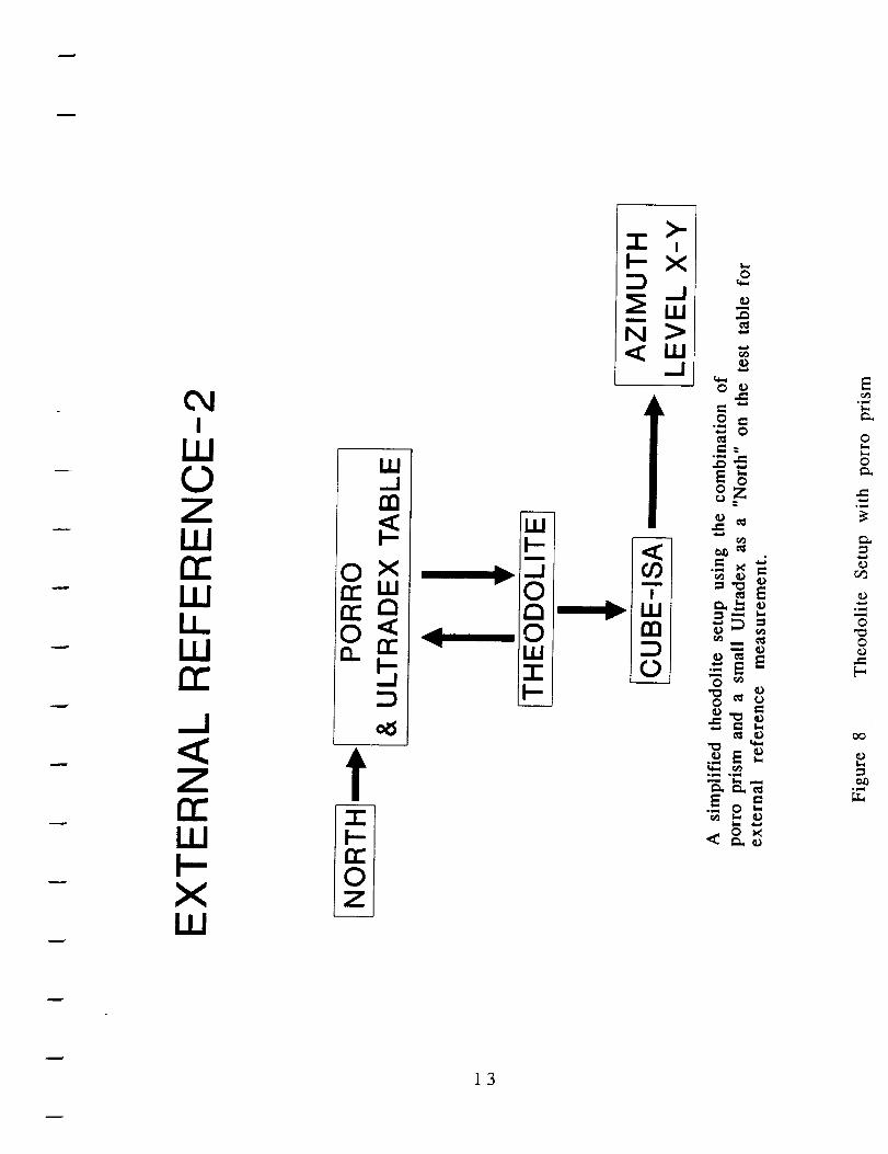
This is a time consuming and difficult operation, and we eliminated
error and saved time by using a combination of the precision
Ultradex table and a porro prism to establish "North" on the test
table top ( see Figure 8 for conceptual drawing).
Three Axis Dividing Head Table
The initial system testing was conducted on a three axis dividing
head table ( see Figure 5). This setup allowed us to adjust the system
azimuth, elevation and roll. The table resolutions in azimuth and
elevation are 5 arc-seconds and adjustment in roll is limited to the
"worm" gear resolution. At each test position, the exact position was
confirmed by using theodolites in all angles. Using this technique, we
were able to complete our first system calibration run before moving
to the newly installed high precision air-bearing rate table.
Air-bearing Table
A high precision air-bearing rate table model 51C manufactured
by Contraves was installed in our laboratory for these tests (see
Figure 6). The table was designed for testing high accuracy mechani-
cal and laser inertial systems. The aerostatic table axis bearing
exhibits very low axis friction and minimizes axis wobble for effec-
tive evaluation of gyro performance. The servo driven table axis
(azimuth) provides precise control of table position which is
displayed at the control console with a resolution of .0001 deg (0.36
arc-sec). The table payload is rated at 800 Ibs in the vertical axis.
The table was installed on an isolation pad to isolate the test stand
from the rest of the building. A 12 inch Ultradex table was mounted
on top of the table for system elevation adjustment. The Ultradex
11

0Z
>-"I- iF- X
.J
N > 0
0
0°_m
0
00
°
II
o 0
ZrrUJ
XW
I--Irrl
]2
Iii0ZUJn,-WU_Illn,-
<Z
Ill
W_Inn
OC
t7-
n-OZ
Ill
m
"_ 0I"70W7"
7- lF- X
..J__,,,N >< W
.J
m
I
Wml ,
w I
0
0 ¢)
0
eZ
_E
°_ °_
EoE,_
O _
E
0
0
o_
C_
r_
©
0
0
b.
13

table model R-13722-3 was manufactured by Absolute Accuracy
Gage Inc. with horizontal recommended load limit of 300 lbs. The
Ultradex table accuracy is better than 0.25 arc-sec with 0.25 degree
incremental resolution.
Table Calibration
A high precision theodolite model-T-2000 and an autocollimator
were used to calibrate the air-bearing azimuth table and Ultradex
elevation table. The spindle axis of the air-bearing azimuth table was
adjusted within 2 arc-sec for 8 different table positions(0, 45, 90,
135, 180, 225, 270, 315). These 8 positions were used for system
calibration operation. The air-bearing table azimuth resolution of
0.0001 deg (0.36 arc-sec) was confirmed by using the combination of
the high precision theodolite and the autocollimator.
The Ultradex table used for elevation movement was aligned to
the local level and the 1/4 arc-sec table resolution was confirmed by
using the high precision theodolite.
Test environment
All tests were conducted in an air-conditioned, temperature
controlled standard laboratory environment. No special attentions
were made to control room temperature better than +/- 2 deg F nor
were there any attempts to control room humidity.
14

IV. RLG Array Descriotion. and Test Configurations
Inertial Sensor Assembly Description
The Inertial Sensor Assembly(ISA) includes three RLG's and
three Sundstrand QA 2000 accelerometers (see Figure 2). For this
testing, the three gyros that were installed into the ISA were
X gyro SN: B2003
Y gyro SN: B4500
Z gyro SN: Z2002
It also includes the High Voltage Power Supply and the current
regulator assemblies needed to start and run the plasma discharges
for the three RLG's. Additional low-voltage support electronics exist
in the system cards that are interfaced to the ISA through two 50-
pin connectors. The RLG's are mounted orthogonally and the three
accelerometers are similarly mounted so their respective axes are
collinear with the gyros. The accelerometer triad is mounted close to
the center of gravity of the ISA to minimize lever-arm effects.
The ISA also has magnetic shielding(50:l) to reduce any
magnetic effects from sensor outputs to values below instrument
stability levels. Typical gyro sensitivity when mounted in the ISA is
0.0002 dph/gauss. The areas where testing is done show field
fluctuations less than 1 gauss for the tests that were conducted for
this gyro evaluation.
The ISA assembly is suspended by eight vibration isolators
that are matched in transfer characteristics to keep the center of
suspension co-incident with the center of gravity and thus minimize
dynamic motion. The isolators are arranged in a symmetric fashion
to aid in balancing the entire assembly. The eight mounting points of
the ISA are arranged such that four are through the top of the
system chassis, and four are through the bottom of the systemchassis.
Ring Laser Gyro Noise Sources
There are three basic noise sources for the RL-34 gyro in this
application: quantization noise, random walk noise and gyro bias
instability noise. Each error appears differently as a function of
testing time and system output (rate or angle). At short test times
for angle measurements the error is dominated by the gyro
quantization, while the gyro random walk error increases as a square
root function of time and the bias instability contribution grows
linearly as a function of time. The overall Noise Equivalent Angle
(NEA) and Noise Equivalent Rate (NER) equations are given as :
15

NEA = +
and
( RWC_/3600 T)2 2
+ (BI*T)
NER = + + (BI)2
where Q is the gyro quantization error in arc-sec, RWC is the gyrorandom walk in deg/root-hr, BI is gyro in-run bias instability indeg/hr, and T is the data sampling time in seconds.
Sigma Plot Generation
One useful method to estimate the quantization, RWC and bias
instability errors for an RLG is to plot the standard deviation of the
gyro output vs integration time. Table 1 shows the first 60 points of
data for B4500 from data file 06-30-91.g (see appendix A for details
on datafile). The first column shows run time in seconds for the 100
seconds/sample data. The second column shows the gyro pulses per
100 second sample. The scale factor (SF) for the RL-34 with X4 logic
is 0.3838 arc-sec/pulse. This SF was used to scale the gyro
pulses/100 sec to deg/hr (column 3). This data represents the gyro
output integrated for 100 seconds. At the bottom of column 3 is
shown the integration time of 100 seconds with a standard deviation
for the 60 points of .0072 deg/hr. Column 4 shows the data
integrated for 200 seconds with a standard deviation for the 30
points of 0.0042. Similarly, the data was integrated into 300 and
400 second samples. The maximum integration time was limited at
400 because longer integration times gave less than 15 samples (an
arbitrary limit for a statistically valid sample size).
A plot on a log-log scale of standard deviation vs integration
time allows graphical analysis of the various noise terms described
above. It can be seen that from the NER equation that on a log-log
plot the quantization noise has a slope of -1, the RWC noise has a
slope of -1/2, and Bias instability has a slope of 0. Figure 9 shows a
graphical estimation of the three errors by drawing the appropriate
slope lines through the data. In order to reduce time and increase
accuracy, a computer program was developed which fits the NER
equation to the data. It still plots out the data and draws the
appropriately sloped lines for visual confirmation of the fit to the
data. Figure 10 show the computer generated lines and the
16

Table IExample of Calculations for a Sigma Plot
Data file: 06-30-91. 9 Gyro SN: B4500 Scale Factor: 0.3838 arc-sec/pulse
Run Time
(see)Gym OmputSN: B4500
Pulses/lO0 see)100 2572
200 2571
30[ 2570
400 2568
500 2569
60( 2564
700 2574
800 2564
900 2569
1000 2569
1100 2568
1200 2568
1300 2569
1400 2567
1500 2571
1600 2568
1700 2568
1800 2566
1900 2569
2000 2572
2100 2567
2200 2567
2300 2568
2400 2570
2500 2569
2600 2566
2700 2570
2800 2568
2900 2568
3000 2571
3100 2569
3200 2565
3300 2569
3400 2568
3500 2570
3600 2570
3700 2568
3800 2567
3900 2569
4000 2568
4100 2570
4200 2567
4300 2567
4400 2571
4500 25684600 2570
4700 2569
480C 2568
490C 256_
5000 2566
5100 25711
5201 2568
5300 2570
540C 2567
55001 2567
5600 2570
5700 25685800 2569
5900 2567
6000 2570
Scaled to
Deg/hr
(deg/hr}9.871;
9_8675
9.8637
9.8560
9,8598
9.8406
9.8790
9.8406
9.8598
9.8598
9.8560
9.8560
9.8598
9.8521
9.8675
9.8560
9.8560
9.8483
9.8598
9.8713
9.8521
9.8521
9.85609.8637
9.8598
9.8483
9.8637
9.8560
9.8560
9.8675
9.8598
9.8445
9.8598
9.8560
9.8637
9.8637
9.8560
9.8521
9.8598
9.85609.8637
9.8521
9.8521
9.8675
9.8560
9.8637
9.8598
9.8560
9.8598
9.8483
9.8675
9.8560
9.8637
9.8521
9.8521
9.8637
9.85609.8598
9.6521
9.8637
Summed 1o
200 se_sample
(deg/hr)
9.8694
9.8598
9.8502
9.8598
9.8598
9.8560
9.8560
9.8617
9.8521
9.8656
9.8521
9.8598
9.8541
9,8598
9.8617
9.8521
9.8579
9.8637
9.8541
9.8579
9.8579
9.8598
9.8598
9.8579
9.8541
9.8617
9.8579
9.8579
9.8579
9.8579
Summed to
300 sec/sample
(deg/hr }
9.8675
9.8521
9.8598
9.8573
9.8598
9.8534
9.8611
9.8573
9.8573
9.8598
9.8547
9.8611
9.8560
9.8573
9.8585
9.8598
9.8585
9.8573
9.8573
Summed to
400 sec/sample
(de(j/hr)
9.8646
9.8550
9.8579
9.8589
9.8589
9.8560
9.8569
9.8569
9.8608
9.8560
9.8589
9.8589
9.8579
9.8579
9.8585 9.8579
Number of,Samples 601 30 20 15
300
0.0032
200
0.0042
100
0.0072Integration Time (see)
Standard Deviation (deg/hr)
400
0.0023
17

I000÷@,I00
I
I _I I I I
6j
[" Jtl/" 6ap] ssauwopueJ oJAO jo 6oT
¢JQ;
E
QJe--I
rlE
i/i
o
oio
01I
Ir,,
o
0
O,
O_I
0
I
LO
0
/d.J
IJ.
I--
o
00ftJ
_5rr
18

('Jq/'Sap) ssaumopueJ oJ_5 _o 6OT
/
/.
ooo÷Q;
o oo o0 0÷
oo0
I
0oo÷QJo0o
u
Q;E-J"t
E
w_
o
o
O_I
ID,.0
0
oiI0tr}ILO0
6J.JP_
b.
,0{
r'_
or}00O0m
_5rr_>-
19

calculated values. Notice that they agree except for the bias
instability value. The computer value is more accurate than the
graphical analysis because the test was not long enough to
graphically determine the bias instability yet the computer can stillestimate the information.
Individual Gyro Information
An RL-34 gyro is generally biased at less than 0.04 degrees per
hour. This is a fixed bias magnitude which does not imply bias
stability, one of the features of RLG technology. Typical RL-34 gyros
have bias stabilities of less than 0.0005 dph, which is more than
sufficient for the their navigational system requirements, but needs
to be better for the DSN pointing application. In-run stabilities of
RL-34 gyros at constant temperature have been as good as 0.00015
dph.
During the gyro evaluation, there was a unique opportunity for
GSD to evaluate the RL-34 gyroscope for the DSN application. We
utilized three RL-34 gyros set aside for our high-accuracy navigation
systems demonstrator. These three units are representative of GSD's
high accuracy RLG development. While all have been tested and
accepted for our navigations system requirements, GSD felt they
came close to the requirements for the DSN application.
Gyro S/N B4500 was built under last year's IR& D program and
has demonstrated 0.00046 dprh random walk, with bias
repeatability of less than 0.0004 dph, one sigma. The bias
repeatability is the residual error left after thermal modeling over
the temperature range of -55 to + 70 degrees Celsius. A significant
portion of this error resides below -10 Celsius, and as such significant
performance improvement is possible for a DSN application. Also
note that turn-on to turn-on bias repeatability at room temperature
has been shown to be within the RL-34's in-run bias stability and is
less than thermal residual bias repeatability.
S/N B4500 is part of constant improvement of RLG technology,
and it has capability for in-run bias stability of less than 0.0002 dph.
This unit is part of our newest series of RL-34 gyros designed under
IR&D funding, which have been better performers than previous RL-
34 gyros built at GSD. They have lower environmental sensitivities,
improved bias performance, and are more producible than previous
RL-34 gyros.
Gyro S/N B2003 was built in 1989, and was evaluated at the
Army MICOM laboratories, as part of our entry into RLG based land
navigation systems and north finding modules. At that time, this
unit demonstrated 0.0005 deg/hr bias repeatability over
temperature, and 0.001 deg/rt-hr random walk coefficient. At GSD
20

this unit has tested to bias repeatabilities better than 0.0007 dph,and RWC of better than 0.00055 dprh. In addition, this unit hasshown in-run bias stability of 0.0002 dph.
Gyro S/N Z2002 was built in 1988 under our IR& D program,and has tested at better than 0.001 dph bias repeatability overtemnperature, while having a random walk of 0.00059 dprh.
These three gyros are representative of our high accuracy RLGprogram at GSD, and all are tested, proven performers which GSDutilized during the gyro evaluation program for DSN applications.They were installed into the ISA as listed below:
X gyro SN: B2003Y gyro SN: B4500Z gyro SN: Z2002
Appendix A includes plots of individual gyro data for each ofthe three gyros. Each of the sigma plots has been marked graphicallyto estimate the random walk coefficient and the in-run bias stabilityfor each gyro. This data was previously provided to JPL underseparate cover on July 10, 1991, including the actual data records ona floppy disk.
21

V. Data acquisition _lnd orocessing descrivtion
The standard input/output port of the navigation system used
for these tests is an RS-232 serial port. The data acquisition
computer used this RS-232 serial port to inte_ogate various system
variables every 100 seconds during the course of a test. These
system-variables include compensated and uncompensated gyro and
accelerometer outputs as well as attitude and navigation variables
like roll, pitch, heading, latitude and longitude. The data acquisition
computer stored all 60 system variables while providing the
capability to plot up to 6 variables real time. The stored datafilenames contain the date of the test and the number of tests started
that day. For example 092091b.dat is the second test started on9/20/91.
All of the detailed data analysis and plots were generated on
an additional computer using a custom software package. Most of
the summary data was tabulated and analyzed using either Lotus
123 or Microsoft Excel. A detailed description of the analysis will be
included in the next section as the processed test data summaries are
presented.
22

VI. Processed test data summary records
Initialization
The gyro bias requirements for the JPL application require the
gyro biases be calibrated to <0.0001 dph. This specification was
based on the need to track a target for 10 hours to within 0.001
degrees-rather than the requirement for intialization of <0.0002 dph.
The long term bias stability (months years) will maintain this
accuracy only with periodic re-calibration. A calibration procedure
was designed that will allow the gyro biases to be periodically
calibrated in a manner consistent with the DSN application. This
procedure entails mounting the system on an indexing table or
equivalent and testing at 4 different positions. From these four
positions, the gyro and accelerometer biases can be determined. To
evaluate if this procedure was plausible, we used it to calibrate the
gyro biases. It is estimated that this 24 hr calibration procedure (6
hrs at 4 positions) will have to be performed monthly to maintain
the bias requirements for the JPL application.
To calibrate the gyro biases, the table was set to 4 positions: 0,
180, 90 and 270 deg. When the rate table is set to 0 deg, the X axis
of the system is North. At position 90 deg, the X axis is East. At
each position, multiple 15 minute alignments were performed for
over 4 hrs. The heading value at the end of each alignment was
recorded. The table below summarizes the four calibration positions.
Table II
Calibration Data at Four Positions
Data File Table Table
Azimuth Azimuth
Degrees Mils
System Number
Output Standard of
Mean Deviation AlignsMils Mils
090691 b.dat 180 3200
09099 la.dat 360 6400
090991 b.dat 90 1600
091091a.dat 270 4800
3200.74215 0.05792 176
6398.79999 0.06929 26
1600.74174 0.14317 46
4898.81603 0.11603 18
To clarify this data, the calibration test performed at the 360
degree position will be examined in detail. This test was performed
for over 6.5 hrs with 26 fifteen minute aligns being performed. The
table below shows the heading for all 26 aligns. These aligns have amean of 6398.800 mils with a standard deviation of 0.0693 mils, or
23

TABLE III
List of Azimuth at Completion of AlignmentDatafile 090991 a.dat
1 6398.715 14 6398.8632 6398.838 15 6398.8313 6398.793 16 6398.8634 6398.876 17 6398.8795 - 6398.729 18 6398.7736 6398.927 19 6398.7057 6398.855 20 6398.8418 6398.732 21 6398.7059 6398.843 22 6398.902
1 0 6398.775 23 6398.6711 1 6398.790 24 6398.8211 2 6398.723 25 6398.83313 6398.747 26 6398.764
Standard Dev. 0.0693 milsMEAN 6398.800 mils
0.0039 degrees. Recall that 6400 mils = 1 revolution. This datafile
(090991a.dat) will be included with the raw data records.
The old bias values for the X, Y, Z gyro were -0.00388, -
0.002112, and 0.00449 deg/hr, respectively. From these four
calibrations runs, the bias corrections for the X and Y gyros were
calculated to be +0.01075 and -0.010845, respectively. The new bias
values of +0.00687 and -0.01296 (x and y, respectively) were
entered and stored into the system to be used in all future tests. The
Z gyro bias was not adjusted for these initialization tests since Z gyro
bias errors do not affect gyro compass accuracy in these positions.
The additional advantage of this calibration procedure is its
ability to determine the boresite error. The boresite error for this
mounting configuration is -0.225 mils. This means that as the table
is set to different azimuth positions, there will be a consistent -0.225
mils difference in the system azimuth output.
With the boresite known and the gyros biased, a test was
performed to evaluate the overall gyro compass accuracy at 8
different table azimuth positions. Table IV show a summary of these
tests. The last column is the azimuth system error representing the
difference between the actual value and the expected value. The
mean and standard deviation for the 8 azimuth errors are
calculated.
24

Data File
Table IV
Summary of Gyro Compass Accuracy at 8 Positions
Table Table System System No ofAzimuth Azimuth Azimuth Azimuth(degs) (mils) Mean (mils) 1 sigma
(mils)- Aligns
091091d.dat 36018090
091191f.dat 270315135
091291c.dat 45225
6400.0000 6399.755063200.0000 3199.791021600.0000 1599.741644800.0000 4799.791065600.0000 5599.81172400.0000 2399.76465
800.0000 799.757194000.0000 3999.83993
0.046380 046080 150980 151180 082540 160840 156220.11582
STDMEAN
AzimuthError(arc-sec)*
11 4.01 1 -3.225 6.7
23 -3.31 7 -7.416 2.124 3.623 -13.1
6.7-1.3
* Azimuth Error = (Table Azimuth - System Azimuth Mean + Boresite) *360/6400*3600
Boresite (mils) -0.22504
Some additional initialization tests were performed at other
table azimuth positions and are summarized on table V. The overall
performance was obtained by analyzing these 14 table positions and
the 8 table positions shown on table 3. These 22 table positions hada mean of -0.82 arc-sec with a standard deviation of 6.1 arc-sec.
25

Table VSummary of Additional Gyro Compass Positions
Data File Table Table System SystemAzimuth Azimuth Azimuth Azimuth(degs) (m i l s) Mean (mils) 1 sigma
(mils_-
No of
Aligns
AzimuthError
(arc-sec)*
091391f.dat
092391 b.dat
360 6400.0000 6399.75715 0.04001180 3200.0000 3199.79099 0.03832
200.0500 3556.4444 3556.23502 0.0726200.1000 3557.3333 3557.13241 0.08962200.1500 3558.2222 3558.02457 0.08043200.2000 3559.1111 3558.90043 0.0772200.2500 3560.0000 3559.82402 0.07599200.3000 3560.8889 3560.71208 0.06746
360 6400.0000 6399.75317 0.04720.1308 2.3253 2.08827 0.051940.1336 2.3751 2.11725 0.050270.1364 2.4249 2.17122 0.046790.1392 2.4747 2.20722 0.057840.1420 2.5244 2.29645 0.05182
STDMEAN
22 3.623 -3.222 -3.222 -4.922 -5.522 -2.922 -9.922 -9.7
8 4.41 1 2.411 6.611 5.812 8.612 0.6
6.0-0.5
For All 22 table azimuthpositions
STD 6.1MEAN -0.8
* Azimuth Error = (Table Azimuth - System Azimuth Mean + Boresite) *360/6400*3600
Boresite (mils) -0.22504
26

The ability to calibrate the gyros in the system to < 0.0002 dph
bias with the above calibration procedure did not prove completely
effective the first time. The data in table IV shows the gyrocompass
accuracy at 8 positions after initially calibrating the gyro biases.
Note that the first four positions are a repeat of those used duringthe calibration. If these tests were considered to be a second
calibration, the X and Y gyro biases should still be adjusted by
-0.00028 and 0.0002 dph, respectively. These small bias errors
remained due to the approximate equations used to calculate the
gyro biases from the calibration data. Because of earlier experiments
with the system software, the biases values required considerable
changes (.01 dph) after the first calibration. Once the system is
calibrated, the monthly changes will be much smaller in magnitude
and the approximate equations will be acceptable to bias the gyros to
0.0001 dph.
Due to the limited test time available on this program, the
biases were not changed and testing continued. This data was later
post processed to correct for the bias errors. Table VI shows the
azimuth error (from table IV & V), the correction based on the bias
errors, and the corrected azimuth error. This reduced the
initialization error by a factor of 2 (to 3.1 arc-sec, one sigma)
showing that the system performance slightly exceeded the expected
limit (see error analysis section).
Even though bias errors were included, they remained constant
during the initialization portion of the tests. Table VII shows a
summary of tests repeated at table position 360 and 180 degs (based
on the corrected azimuth error from table VI). At the 360 deg
position, the azimuth error had a standard deviation of 0.4 arc-sec
over a 13 day period. Even though this standard deviation is slightly
lower than expected (see error analysis section), it indicates an
extremely stable gyro bias.
27

X Bias ErrorY Bias Error
Datafile
Table VI
Azimuth Error Corrected
-0.000280.0002
Table Azimuth
(degs)
for Bias Errors
Azimuth Error* Azimuth Corrected AzimuthCorrection
(arc-sec) for bias Error** Error***(arc-sec) (arc-sec)
091091d.dat 360.00 4.00 3.63 0.37180.00 -3.20 -3.63 0.4390.00 6.70 5.08 1.62
091191f.dat 270.00 -3.30 -5.08 1.78315.00 -7.40 -1.03 -6.37135.00 2.10 1.03 1.07
091291c.dat 45.00 3.60 6.16 -2.56225.00 -1 3.1 0 -6.16 -6.94
091391f.dat
092391 b.dat
360.00180.00200.05200.10200.15200.20200.25200.30360.000.13080.13360.13640.13920.1420
3.60-3 20-3 20-4 96-5 50-2 90-9 90-9 704 402.406.605.808.600.60
3.63 -0.03-3.63 0.43-5.15 1.95-5.15 0.19-5.16 -0.34-5.16 2.26-5.16 -4.74-5.17 -4.533.63 0.773.64 -1.243.64 2.963.64 2.163.64 4.963.64 -3.04
STD 6.08 3.09MEAN -0.82 -0.40
* From table IV & V
**Azimuth Correction =Table_pos -ATAN((11.37"S IN(Table_Pos)+ybias)/(11.37*COS(Table_Pos)+Xbias))
*** Corrected Azimuth Error = Azimuth error - Azimuth Correction
28

Table VII
Summary of Repeated Alignment Tests
Datafile Corrected azimuth error *Table Azimuth Position
(arc-sec)360 180
091091d.dat 0.37 0.43091391f.dat -0.03 0.43092391 b.dat 0.77
Standard Dev. 0.40
* From table Vl
Error Analysis of Initialization tests
The initialization is a gyrocompass operation where the two
level gyros (Gyro X and Gyro Y) are used to measure the horizontal
component of Earth's rate. The Azimuth angle is equal to the
arctan(GyroY/GyroX). Depending on length of time spent gyro
compassing, the accuracy will improve and can be predicted from the
NER for each gyro. A propagation of error analysis can predict the
uncertainty in azimuth based on the NER of the X and Y Gyro. This
was done in Table VIII.
Since there was a substantial difference between the RWC of
the X and Y gyros, the uncertainty in azimuth should vary depending
on which gyro is primarily used to gyrocompass. Table VIII shows
the predicted uncertainty in azimuth as of function of azimuth.
There is fair agreement with actual system azimuth uncertainties.
Note that table azimuth positions 360 and 180 show a lower noise
than the 90 and 270 azimuth positions. This is because at the
360/180 positions, the gyrocompass is dominated by the Y gyro. At
the 90/270 positions, the gyro compass is dominated by the X gyro.
Since the Y gyro has lower noise in 15 minute samples then the X
gyro, the gyrocompass noise is lower at the 360/180 positions
compared to the 90/270 positions. Future tests were initialized near
360 table azimuth to take advantage of the reduced noise in this
orientation.
29

Table VIII
Initialization Error Based on Gyro Noise Model
Gyro XQuantization Noise (arc-sec)*** 1.2
RWC (dprh)*** 0.0008Bias Instability (dph)*** 0.0002
Gyro Y1.2
0.00030.0002
NER for 15 minute alignment time 0.001 70 0.00083
Table AzimuthUncertainty in Azimuth
Predicted* Actual**
(Mils) (Mils)
36O18090
27031513545
225
Mils0.0740.0740 1520 1520 1200 1200 1200 120
0.0460.0460.1510.1510.0830.1610.1560.116
Horizontal Earth's Rate (dph) at BGSD Latitude = 11.37 deg/hr*Predicted = ((SigmaX*SIN(table))^2+(SigmaY*COS(table))^2)^0.5
*180/PI()*3600/ERH/3600/360*6400** From Table IV*** Based on sigma plot analysis with system in current configuration
The above analysis also predicts what the ultimate
gyrocompass accuracy will be for longer gyrocompass times. The
gyro noise for time periods longer than 4-6 hrs is dominated by the
bias stability of the gyro. If a 0.0002 dph bias stability and 0.0003
dprh RWC gyro is used to gyrocompass for 6 hrs, the expected gyro
and azimuth noise are 0.00023 dph and 4.2 arc-sec, respectively.
Taking another look at the data on table VI shows there is fair
agreement to the actual data. The "Azimuth Error" shows a 6.1 arc-
sec noise (sigma) and the "Corrected Azimuth Error" shows a 3.1 arc-
sec noise. Both of these numbers are close to the expected azimuth
noise with the "Corrected Azimuth Error" even slightly better than
expected.
3O

System turn on and off repeatability test
The system was locked at table position 3200 mils (south) and
tested for on-off repeatability. The system was turned off for 24 hrs
in between each turn on as required in the statement of work.
During the turn on periods, gyro compass data was recorded for 8 hrs
and the mean value calculated. The results were :
1st turn on and system heading : 3200.830 mils
system off for 24 hrs
2nd turn on and system heading : 3200.852 mils
system off for 24 hrs
3rd turn on and system heading : 3200.845 mils
This data shows that the system has excellent repeatability
with a 2.3 arc-sec 1 sigma.
Initialization Testing Conclusion
The statement of work's objective for initialization translates to
an accuracy of 3.7 arc-sec (0.0002 deg/hr bias error at BGSD
latitude). When the data is post processed to remove the remaining
small bias errors, the initialization results yield 3.1 arc-sec, 1 sigma.
This indicates that the two gyros whose input axes lie in the level
plane clearly have bias stabilities < 0.0002 deg/hr. It further
indicates the potential of the BGSD RL-34 RLG-based pointing system
to initialize to within the 0.001 degree angular objective.
31

Blind Acauisition T_tin_,
The first series of acquisition tests were 20 degree azimuth
rotations at 0 degree elevation. In this test series, the experiments
were conducted by rotating the air-bearing azimuth table from
either east-to-west or west-to-east for exact 20 degree angles at
various rotation rates of 0.5 deg/sec, 0.2 deg/sec, 0.07 deg/sec, and
0.05 deg/sec rates as required by the statement of work.
The test data was recorded in the form of system heading,
pitch and roll information. The objective was to compare the system
heading raw data before and after 20 degrees air-table rotation. The
azimuth error was defined as any heading deviation from 20 degreesrotation as shown below:
Azimuth error= Abs.Value{headingl-heading2}-20 degrees
where heading 1 is the system heading reading before the 20
degrees rotation and heading 2 is the system heading reading after
20 degrees rotation.
The system information is updated every 100 seconds with our
current data acquisition design and no attempt was made to change
the system readout software for instant update after rotation.
A summary of these test results is given in Table IX, showing
one sigma azimuth error as a function of azimuth rotation rate. The
one sigma of these measurements clearly demonstrated that the
system error is a function of rotation rate. This is consistent with the
theoretical noise equivalent angle (NEA) model as predicted in the
NEA equation (see the ring laser gyro noise section).
In addition to the theoretical NEA error, there was an air-
bearing oscillation problem at the end of table rotation when the
table was rotated at low rotation rates. By hand locking the table at
the end of rotation, the table oscillation problem was eliminated and
the one sigma of the measurement was improved from 3.02 arc-sec
to 2.29 arc-sec which represented an improvement of 25%.
32

Table IX
rotation rate :
10.5 deg/sec
system pointing
error (arc-sec)
MEAN
SIGMA
E-W
W-E
-0.75
0.41
0.21
-0.75
O. 79
0.23
0.81
0.61
E-W
W-E
0.81
-0.37
-0.17
-1.93
-1.73
-1.15
-1.35
-0.37
-0.55
-0.57
-0.35
-0.57
-0.37
-0.34
0.78
rotation rate
0.2 deg/sec
system pointing
error (arc-sec)
1.99
0.99
0.79
0.99
0.79
1.39
0.01
1.19
-0.75
-0.17
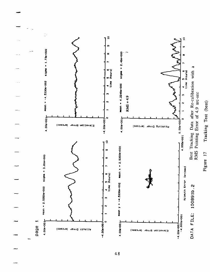
-1.55
-2.33
-1.55
-2,15
-2.13
0.01
-0.75
-0.19
1.34
E-W
W-E
rotation rate :
0.07 decj/sec
system pointing
error (arc-sec)
1.19
3.35
3,93
-2.71
-4.27
1.8
2.57
-1.91
-3.29
0.41
3.35
5.31
0.81
3.02
E-W
W-E
hand locked the table
at end of rotation
rotation rate:
0.05 deg/sec
system pointing
error (arc-sec)
1.79
4.51
3.09
0.01
-1.93
0.03
0.03
0.99
2.17
1.39
-3.89
-2.91
-4.53
-0.77
1.57
-1.33
-1 .15
2.53
-1.73
-0.95
-0.05
2.29
Table IX : Summary of target acquisition test results for 20
deg azimuth rotation at 0 deg elevation. The data is given as systempointing errors resulting from 20 deg azimuth rotation. In both rotation
directions, east-to-west(E-W)and west-to-east(W-E), there is no significantdifference in the pointing errors. The near "zero" mean value of these
measurements shows that the system input vertical axis is well aligned withthe rotation axis of air-bearing table.
In all these tests, the near "zero" mean value suggests that the
system vertical axis is well aligned with rotation axis of air-bearing
table and the test data also indicates that there is no significant
difference between east-to-west and west-to-east rotation directions.
Further analysis of the test results by removing the known table
error showed the true system error is only 0.55 arc-sec, for the
rotation rate of 0.5 deg/sec. This compares favorably with the
statement of work objective of 0.36 arc-sec.
33

0 2 - 42 0 2 "t- 42- (Ymeasured- system
2
az-table
0 az-table = 0.36 arc-sec.
I3 measured = 0.78 arc-sec
0 = 0. 55 arc-secsystem
Compound Angle Acquisition Tests
To demonstrate the system repeatability in the blind target
acquisition mode, we decided to conduct the tests at the worst case
scenario by rotating the system 20 degrees in air-bearing table to
simulate the azimuth rotation and +/- 60 degrees in Ultradex table to
simulate the elevation rotation for northern and southern
hemispheres. One of great strengths of a ring laser gyro is the
inherent precision scale factor with no apparent upper rotation rate
limitations. And the gyro often shows the scale factor is better than 1
ppm from near zero rotation rate to 2 revolutions/sec.
The blind target acquisition requirement for this Deep Space
Network (DSN) gyro evaluation is 0.36 arc-sec accuracy over 20
degrees rotation which corresponds to a gyro scale factor linearity of
5 ppm. This is a "relative easy target" to meet in a ring laser gyro
based navigation system except where there is a short time duration.
The gyro angular resolution(Least Significant Bit or LSB) limits the
angular accuracy that can be achieved in short time intervals(see
previous discussion of noise equivalent angle). The RL-34 gyro
based system used in our tests has an LSB resolution of 0.38 arc-
sec/pulse, meaning a one pulse error is the entire budget for this testseries.
Fortunately the LSB of the gyro is only limited by how we
sample the gyro analog output. For the purposes of present
production navigators, the existing 0.38 arc-sec sampling works
acceptably. However, we recognized that space and ground based
pointing applications require Bendix to improve our current RL-34
resolution. We developed circuitry in early 1991 that modifies the
RL-34 resolution from 0.38 arc-sec/pulse to 0.05 arc-sec/pulse
which will be able to meet the DSN pointing requirements (see
Recommended Alternatives to Improve Performance Section)
All the test results were recorded as a system outputs of heading,
pitch and roll. The system data is updated every 100 sec and data is
compared between the system reading before moving and after
moving for both heading and pitch. The repeatability of the test is
presented as an azimuth error and pitch error. The definition of
these errors are given as the following:
34

Azimuth error= AbsValue{headingl-heading2} - 20 deg - mean value
Elevation error= AbsValue{pitchi-pitch2}- 60 deg - mean value
where headingl is the system heading reading before the rotation
operatio_ and the heading2 is the system heading reading after the
rotation operation, and the same is true for the system pitch reading.
Table X showed a typical compound angle acquisition test
results. The data recorded as system's heading, roll and pitch in the
unit of mils. The compound angle was made by rotating air-bearing
table 20 degs and Ultradex table +60 degs. In Table X, the delta
heading is the absolute value of heading difference before and after
rotations minus 20 deg azimuth rotation, and the azimuth error is by
removing the mean value generated in the delta heading. Similar
mathematical operation is also applied to the pitch data to generate
the elevation error, then, the overall system pointing error is plotted
in both azimuth and elevation errors as shown in Figure 13 and
Figure 14.
The mean value represents a constant misalignment/boresite
artifact that was removed in the post processing. When the rate
table and Ultradex were installed, they were leveled and aligned to
true North as previously described. When the navigation system was
mounted onto the rate table/Ultradex, no fine adjustments were
provided to mechanically align the system input axis to the rotation
axis of table/Ultradex, thereby creating a fixed mean value in angle
which would need to be removed later.
During the initialization and initial acquisition tests (with only
azimuth rotations), the data was corrected for the azimuth boresite.
This was straightforward since the azimuth boresite error was a
constant value with no cross coupling terms. This was expected since
the rate table was leveled to within several arc-sec. As the table was
rotated, the rotation was truly about system azimuth (remember the
system azimuth is defined as the angle from North in a level plane).
35

TESTPOINTS
TABLE X
DELTA AZIMUTH DELTA ELEVATIONHEADING HEADING ERROR ROLL PITCH PITCH ERROR
MILS ARC-SEC ARC-SEC MILS MILS ARC-SEC ARC-SEC
1 5866.432 6222.593 5866.434 6222.615 5866.44
6 6222.627 5866.448 6222.6210 5866.45
11 6222.6212 5866.45
MEAN
SIGMA
123.22122.43125,40124,01125.20124.61124.80123.62124.41124.61
124.230.87
-1.01-1.801.17
-0.22
0.970.380.57-0.61
0.180.38
-0.88-0.43-0.87-0.42-0.87-0.42-0.87-0.42-0.87
-0.42-0.87
-O.O81066.62
-0.081066.63
-0.08
1066.63-0.08
1066.63-0.08
1066.63-0.08
7.517.308.887.89
7.407.166.927.40
8.998.64
7.81
0.72
-0.30-0.511.070.08
-0.41-0.65-0.89-0.40
1.180.64
TABLE X: Typical compound angle acquisition test results.The data was recorded as system's heading, roll and pitch in the unit of mils asa result of repeating compound rotation of 20 deg azimuth and +60 degelevation. For the first test point, the system box is located at air-bearing table350 deg and Ultradex table 0 deg. The second test point is for system box locatedat air-bearing table 330 deg and Ultradex table +60 deg. The third test pointwas repeated at the same location as the first test point, and so on for the rest
of test points.
During the initialization and initial acquisition tests (with only
azimuth rotations), the data was corrected for the azimuth boresite.
This was straightforward since the azimuth boresite error was a
constant value with no cross coupling terms. This was expected since
the rate table was leveled to within several arc-sec. As the table was
rotated, the rotation was truly about system azimuth (remember the
system azimuth is defined as the angle from North in a level plane).
The more complicated problem to be post-processed was the
effect that boresite errors have on azimuth, elevation, and roll with
an Ultradex elevation(i.e, target acquisition). Since the rotation axis
of the Ultradex is not coincident with the pitch axis of the system, as
the Ultradex was rotated, a component of that rotation was coupled
into the system azimuth and roll. Figures 11 & 12 show the system
azimuth and elevation errors versus Ultradex elevation. These errors
were caused by the inability to mechanically align the system to the
36

I.
UJ
=PE_N
E¢D
>,
Error Between
Azimuth
5O
0
-50
-100B
Ig
-150'
-90
System Azimuth and Table
during Ultradex Elevation Changes
[][]rnmBil[][] W
• i [] mm Bin
[][]
[] Elrn
nl
[] BB
-4_ 0 45 90
Uitradex Elevation (deg)
Figure 11 Azimuth Error Due to Boresite Errors
I.
ul
C A
o o
w
E
System10
Error BetweenElevation and Ultradex Elevation
8 ....................................................
6 ................................. _._ .............
4 : .......... . ram Brn
2 =- ............. : [] reBEl•[]
[][]
0 =- ............... [] ............
-2 Big [] .................................: _ .......[][] ra
-4 ....... " =
ram
-6' " ................................
-8 "- mr_ .......................................
-10' • . . .
-90 -45 0 45 9O
Ultradex Elevation (deg)
Figure 12 Elevation Error Due to Boresite Errors
37
-"'7"
air-bearing table/Ultradex. When the system was rotated to a rate
table azimuth and Ultradex elevation, the system reads out a certain
attitude. When the system was re-initialized at this position, the
system still read out the same attitude. The system's ability to locate
attitude was very repeatable throughout the testing.
To use this system for the final DSN pointing application, the
above results indicate that an alignment between the antenna and
the system must be performed. There are two options which will
solve this problem. Mechanical adjustments can be provided to allow
alignment of the system to the antenna or a transformation matrix
can be developed that will transform the system coordinate system
to the antenna coordinate system. Both options require additional
investigation to determine which is best suited for the DSN pointing
application. Since the target acquisition data showed that the system
has excellent repeatability, then with proper adjustments either in
mechanical alignment or transformation matrix operation the final
result will have no impact to the DSN application.
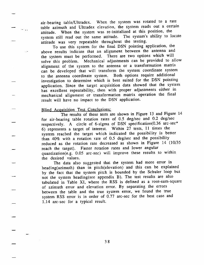
Blind Acquisition Test Conclusions:
The results of these tests are shown in Figure 13 and Figure 14
for air-bearing table rotation rates of 0.5 deg/sec and 0.2 deg/sec
respectively. A circle of 6-sigma of DSN specification(0.36 arc-sec*
6) represents a target of interest. Within 27 tests, 11 times the
system reached the target which indicated the possibility is better
than 40% with a rotation rate of 0.5 deg/sec and the possibility
reduced as the rotation rate decreased as shown in Figure 14 (10/35
reach the target). Faster rotation rates and lower angular
quantization(e.g. 0.05 arc-sec) will improve these results to withinthe desired values.
The data also suggested that the system had more error in
heading(azimuth) than in pitch(elevation) and this can be explained
by the fact that the system pitch is bounded by the Schuler loop but
not the system heading(see appendix B). The test results are also
tabulated in Table XI, where the RSS is defined as a root-sum-square
of azimuth error and elevation error. By separating the errors
between the table and the true system error, we found the true
system RSS error is in order of 0.77 arc-sec for the best case and
1.14 arc-sec for a typical result.
38

'11'
4'
m
8t,_
m., _.
• i' 5.....:.----!_----'-'---......."............_o_
LL!
!
.'t
I I I I I I_
CO C_ "1-- 0 _ 04 _'0! i i
(O:JS-OI:IVNI) 1101::1199NOIIVA37:I
_ °i _
8.. _'_
_ _N._
. __&e
_ ___._
£
-!
o_
e-0
.<
°_,,q
39

•........ • ._ ..........i
4'
.,,_-
-CO
A
o-OJ lil
!
=o
-o==ILl
-'T TI--
.CO!
_'_d"I
I I I I ICO 0,,I _ 0 "_ 0,,I O0
I ! I
(O=l$-Ol:lV NI) I:101:1t:!:1NOIJ_VA37=I
(.9LUI:1
O(D-t-
Z_o
>LU,_111
L9
II.Jii
L9JJ-i
?5>U.3J3
I
c_<D
°_,,_c_
©
O
c_
c_
O
c_
O
cg
c_
E-
O
¢3<
E-
LT.
m
4O
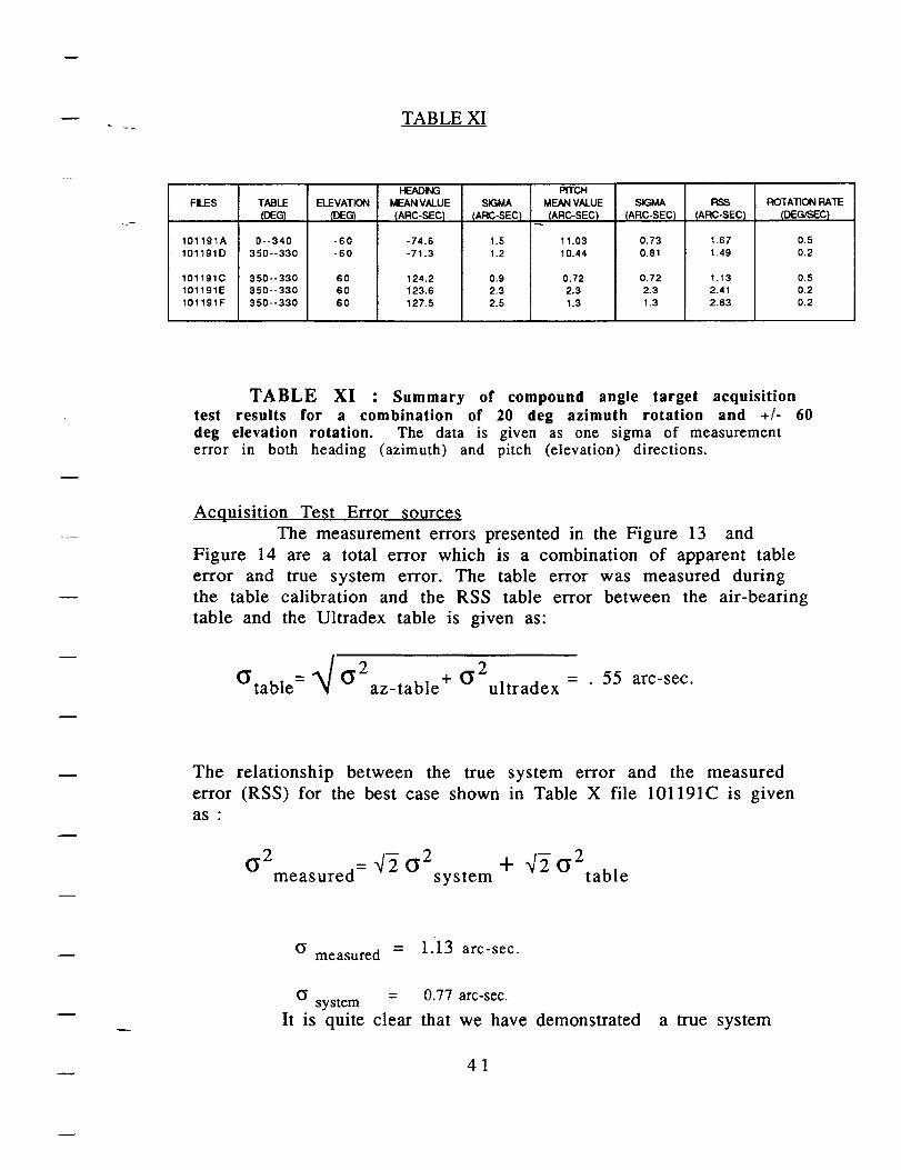
TABLE XI
FILES
101191A
101191D
101191C
101191E
101191F
TABLE
(DEG)
0--340
350--330
350--330
350--330
350--330
ELEVATION
(DEG)
-60
-60
60
60
6O
HEADING
MEANVALUE
(ARC-SEC}
-74.6
-71.3
124,2123.6
127,5
SIGMA
(ARC-SEC)
1.5
1.2
0.9
2.3
2.5
RTCH
MEAN VALUE
(ARC-SEC}
11.03
10.44
0.72
2.3
1.3
SIGMA
(ARC-SEC}
0.73
0.81
0.72
2.3
1.3
RSS
{ARC-SEC)
1.67
1.49
1.13
2.41
2.83
ROTATION RATE
(D_C_VSEC)
0.5
0.2
0.5
0.2
0.2
TABLE XI : Summary of compound angle target acquisition
test results for a combination of 20 deg azimuth rotation and +/- 60deg elevation rotation. The data is given as one sigma of measurementerror in both heading (azimuth) and pitch (elevation) directions.
Acquisition Test Error sources
The measurement errors presented in the Figure 13 and
Figure 14 are a total error which is a combination of apparent table
error and true system error. The table error was measured during
the table calibration and the RSS table error between the air-bearing
table and the Ultradex table is given as:
0 2 (3.2Otable = az-table + ultradex = " 55 arc-sec.
The relationship between the true system error and the measured
error (RSS) for the best case shown in Table X file 101191C is given
as "
0 .2 - _/2 0 2 q- "42 0 2measured- system table
O measured = 1.13 arc-see.
0 = 0.77 arc-see.system
It is quite clear that we have demonstrated
41
a true system
error of 0.77 arc-sec RSS for combination of azimuth and elevationerrors. However, for a typical blind target acquisition measurementthe true system error is on the order of 1.14 arc-sec RSS. Again, it isimportant to note that faster rotation rates and decreased gyroquantization will reduce this error to within the objective of 0.36arc-seconds.
From our previous sigma analysis-;,the values of quantizationerror, random walk and in-run bias stability were 1.2 arc-sec, 0.0003deg/rt-hr, 0.0002 deg/hr, respectively, and the calculated NEA forour gyro is on the order of 0.52 arc-sec which is in fair agreementwith our best case result of 0.77 arc-sec.
By breaking down the error components in the NEA equation, itis quite easy to realize that the gyro quantization error is thedominant error source in our blind target acquisition operation. Byimproving the gyro quantization error to 0.05 arc-sec, we can make agreat impact in this measurement. A quick calculation shows that theimproved NEA shall be on the order of 0.18 arc-sec which is betterthan the stated objective.
The NEA equation also explains why the one sigma of themeasurement is larger at low rotation rates. At low rotation, itrequires more time to complete the 20 degree rotation so that thegyro random walk error term starts to contribute as a square root oftime and eventually dominates the error term. It is therefore helpfulto move the antenna as fast as possible, so that the system resolutionis limited by quantization error and this error is fairly independentof rotation rate.
Inertial Sensor Assembly Orientation Stability
Since the system is mounted on 8 elastomeric isolators, there is
some concern about the mechanical alignment of isolators in the high
elevation orientation. To initially test the mechanical stability of the
isolators, we elevated the system to 40 degrees and used a theodolite
to measure any possible angular changes. The test results showed no
significant change in angle in this setup which implied that the
system mechanical stability is better than one arc-sec. However, in
cold start up conditions, when the system is gradually warming up,
we observed system changes in pitch and small offsets in heading.
The measured results are given in Table XII, and the system
temperature warm up profile is shown in Figure 15. The sagging
stops when the system reaches thermal equilibrium and since most
of our tests are conducted in thermal equilibrium and level, this
finding had no effect on our measured results. This mechanical
instability is only present during a cold start up, therefore it will
have no impact on the DSN application.
42
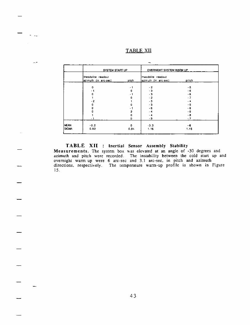
TABLE XII
SYSTEM START UP OVERNIGHT SYSTEM WARM UP
theodolite readout
azimuth (in arc-sec) pitch
0 -1
-1 0
0 -1
1 0
-2 1
0 0
0 -1
0 2
1 0
-1 0
theodolite readout
azimuth (in arc-sec 1
-2
-3
-3
-2
-3
-3
-6
-4
-4
-3
pitch
-5
-6
-6
-7
-4
-5
-6
-6
-8
-7
MEAN -0.2 0 -3.3 -6
SIGMA 0.92 0.94 1.16 1.15
TABLE XII : Inertial Sensor Assembly Stability
Measurements. The system box was elevated at an angle of -30 degrees and
azimuth and pitch were recorded. The instability between the cold start up andovernight warm up were 6 arc-sec and 3.1 arc-sec, in pitch and azimuth
directions, respectively. The temperature warm-up profile is shown in Figure15.
43

O0
(0 "6_0u!)3WfllVW3d_31 _31ShS
O
-,r-n-
O-r
-00Zm
v
w
0_D
J
0
0o_
o
©
E
E
E
E
©
6_
E
44

Target Trackinfl Tests
Once the target is acquired, the goal is to track within 0.001
degrees (3.6 arc-sec), rms, for 10 hours. To evaluate the system's
ability to track a target, the system was held stationary on the rate
table. Any change in system attitude output was an error since the
actual attitude of the system was not changing (other than small
changes due to the isolator temperature sensitivities described
earlier). The system maintained this constant attitude by
transforming the inertial inputs from the gyros and accelerometers
to a fixed Earth coordinate system. This essentially removes Earth's
rate from the gyro inputs and gravity from the accelerometers.
Calibration
Previously during the initialization testing, the X and Y gyro
biases were determined with the calibration procedure. At the time,
the Z gyro bias was not changed because it did not affect the
initialization testing. The Z gyro bias errors only affect the azimuth
output during the 10 hr tracking tests. Upon starting the tracking
tests, an acquisition software error was found that limited the length
of the tracking test that could successfully be performed. While
debugging this problem, these short tracking tests were analyzed and
a Z gyro bias error was observed. The bias was changed 4 times over
this 2 day period and the table below shows these changes.
Table XIII
Z gyro bias changes made during
acquisition software corrections
(deg/hr)
Old Bias Correction New Bias
0.00449 0.00450 0.00899
0.00899 0.00200 0.01099
0.01099 0.00200 0.01299
0.01299 -0.00150 0.01149
At this point, a weekend test was set up to execute multiple 10 hr
tracking tests. These tests comprise the first 6 tracking tests
(datafile: 092091a.dat and 092591b.dat). These tests all showed a Z
gyro bias error of about 0.0009 deg/hr. It was realized that a
complete re-calibration should be performed before any additional
tracking tests were run. At this point various other experiments
were performed, including the acquisition tests.
45

On 10/4/91, a Friday, a calibration test was performed overthe weekend in preparation for some additional tracking tests. Theactual test was about 24 hours long, 6 hrs at the four positions (0, 90,180, 270). The data is shown in below.
Data File
Table XIV
Table TableAzimuth Azimuth
Degrees Mils
System Number
Output Standard of
Mean Deviation Aligns
Mils Mils
100491e.dat 180 3200
360 6400
90 1600
270 4800
3199.86725 0.03291 17
6399.70531 0.04676 16
1599.59889 0.18183 17
4799.99072 0.12124 16
From this data, the X and Y bias corrections were changed for the
first time since the initialization testing. Also, the Z gyro bias was
calculated by knowing that the RSS of all three gyros must equal
Earth's rate. The changes are -.00219, -.00090, and -0.00124 deg/hr
resulting in a final bias of 0.00468, 0.01385 and 0.01273 deg/hr for
gyros X, Y and Z, respectively. A tracking test was performed and a
small (0.00036 deg/hr) bias error was still present for the Z gyro.
This was corrected by changing the Z gyro bias to 0.01309 deg/hr.
The last six tracking tests all had the same bias values.
Tracking Test Results
A total of 12 tracking tests were performed to evaluate the system's
performance. After the first 6 tests, the system was re-calibrated as
described above. Figure 16 shows a typical test and figure 17 is the
best of the 12 tests (after re-calibration). These plots show the
azimuth, elevation and pointing errors versus time and azimuth error
versus elevation error. The pointing error was calculated by takingthe RSS of the azimuth error and elevation error. The overall
performance of each test was determined by taking the RMS of the
pointing error. The plots of the other 10 tests are included in
Appendix C.
Table XV summarizes the results for all 12 tracking tests. The
first 8 tests were performed at 0 deg azimuth and 0 deg elevation.
The ninth test performed incorporated all three phases of testing for
the DSN application. An initialization was done (340 deg azimuth and
0 deg elevation) and was followed by a blind target acquisition
46

w
Q301tOC1
OOO÷QOI
|
g0E
m
O4-I
P1
|
t-
|
[oas:Je) JoJJ:i uo;:ieAa[3
I I I_ I I I I
0q=0
0t
P_
(.
0
lI
¢q
00@000
!
|
|.=m
=" II
I
I I I I
O
o. o@w (3as:Je) JOJJ_ _Ut _U_Od I
0 • " 00 0
miv)
¢D
I
x
CQmZ
0I
I
C10
I
!
00@
00
I I I I I I I I
(=as_Je) JO,JJ3 u0_e^a[3
o
o
00O
0
!
i
C3I...
0
._=_
O
o_=_
c_
c3
U¢.
(=o(=
g ","
5 m
01O
/d...1
b_
F--
o
[..,
°_,,q
4?
OOO÷411q.4_)
,4I
E
ID
OOO@4pOfa_m
l
COG;E
I
O
QJ ÷c_fO oOL
OOO4.ID
l
qEOI
OOIOO
_rI
I
C
I
o.4-AIOO
_r
I I, , i
, I I I
(:as:Je) JOJJ3 uoT_e^a(]
! I I _d I I I
(:O$_Je) JOJJ_ u_nw_zy
O
O_
CD
I..
O
6E
O
?IuOO
I
O
P_
f.
O
1of
O
?IOO
I
OOO@OOILl
I
x
_PE
OOIQO
It)
qrI
i
C_pi/i
00÷0'"1_r
0 II
I l 1 l I I I l 1 I'_I
(3_s=J_) JOJJ:l _uT_UTOd00 0
0
004-
I I I I i I I I I
04,
1 (:;liOJi) JOJJ21 UOt _e^;)[300
0
I
o
_r!
0
m
r_
I.
_r_
llJ
t-
o
°_ °_._
C_
Cu_0_l_
AUIinul..
C.
L
b ru
OO
._/I-..4
LI.
48

(20 deg. rotation & 60 deg. elevation change), which was followed by
a 10 hr tracking test. The last 3 tests were initialized at 60 deg
elevation followed by a 10 hour tracking test.
Table XV
Tracking Error RMS Values (arcsec)All value in arc-sec
Datafile RMS of RMS of RMS of Test DescriptionAzimuth Elevation Pointing
Error Error Error
(arc-sec) (arc-sec) (arc-sec)
092091a.dat 13.0 2.9 13.2
092591b.dat
100891b.dat
100991b.dat
101091a.dat
AverageMinimum
Maximum
17.6
20.1
12.4
18.7
13.6
10.8
4.611.2
17.2
10.4
12.9
13.5
4.6
20.1
4.4
1.7
4.0
3.6
2.1
2.7
1.7
3.8
3.0
3.7
3.9
3.1
1.7
4.4
17.8
19.9
12.818.8
13.6
11.2
4.9
11.8
17.4
11.0
13.5
13.84.9
19.9
Aligned and tracked at 0 deg heading/0 deg elevationm
R
ii
w
n
Recalibrated
Aligned and tracked at 0 deg heading/0 deg elevationI
Aligned at 340 deg heading, 0 deg elevation, trackedat 0 deg heading, 60 deg elevation
Aligned and tracked at 0 deg heading, 60 deg elevation
Aligned and tracked at 0 deg heading, 60 deg elevation
Aligned and tracked at 0 deg heading, 60 deg elevation
The first 6 tracking tests displayed characteristics of the
consistent azimuth gyro (Z gyro) bias error. Figure 18 shows an
overlay of the azimuth errors for the first 6 tests. Note that for the
first 6 hrs all the azimuth errors increased, indicating an uncorrected
gyro bias (about 0.0009 deg/hr). After this time other errors start to
appear (coupled variables) and the error analysis is not
straightforward. Computer analysis and modeling could be
performed to model the cause of these longer time period errors.
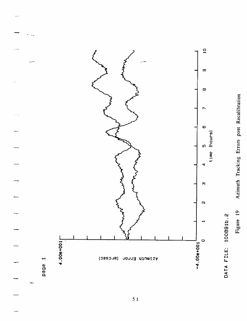
As described earlier, the system was recalibrated before thelast 6 tests. The next two tests showed that the calibration was
successful and the dominant Z gyro bias error was removed. Figure
19 shows an overlay of azimuth errors for these two tests. Note that
there is no initial increase in the azimuth error as previously evident
in Figure 18 These two tests showed lower RMS values compared to
the previous 6 tests that had a Z gyro bias error. The first 6 tests
had a mean RMS pointing error of 16 arc-sec while the latter two
tests had a mean RMS pointing error of 8 arc-sec. Though this is
49

rocL
OO÷
OO
_t
o
O1
(Z)
t_
143
L
o
@3E
4.$
m
I I I I o
Oo÷
O(oasDJe) JOJJ3 q_nw_zv o
I
to
O0d
O
0_O
_J
b.
<[H-
rn
_5
_5
_Jw
O
O
Ld
o0
(J
EN
O
©
oo
@J
5O
Ct)
O.
I
00+U00
I I I _11 I
(_)Bg3JE) JOJJ 3 q%nuJt ZV
o
oi
rn
t',,
o
E.e,4
fel
0
00+W
00
_rI
nJ
n
E)C)C)
..JI-4
I.L
I---
r-_
o
.c)
_s
o
o
o,.._
°_-qN
¢)
° _...q
51

based on only two tracking runs (20 hours of data), this 8 arc-sec
RMS value is a better representation of the system's overall
capability.
The last 4 tracking tests were all performed at 60 deg
elevation. At a non-zero elevation, a combination of two gyro
outputs ( X and Z) principally determine the azimuth reading. The 4
tests did not show any indications of-gyro bias errors (the azimuth
error did not drift consistently), but they did have accelerometer
errors (large Schuler oscillations on the azimuth error). Figure 20
shows the azimuth errors for these 4 tests. Note the larger Schuler
oscillations caused by accelerometer errors. The RMS error for these
tests has a mean of 13.5 arc-sec. As will be discussed in the future
recommendation section, pseudo-g computations should reduce the
Schuler oscillations and the data should approach the expected 8 arc-
sec value.
All of the previous tracking discussions were concerned with
the azimuth error. The elevation error is consistently lower due to
the stable Schuler oscillations that bound the error (see appendix B).
The elevation RMS pointing error currently meets the goal of 3.6 arc-
sec/10 hrs. Table XV also shows the distribution of pointing errors
between azimuth and elevations.
Error Analysis for Tracking
Given gyros that have 0.0003 deg/rt-hr RWC, and 0.0002
deg/hr bias stability, a noise limited prediction calculation can be
made for the system. The NER and NEA for a 10 hour test will be
0.00022 dph and 7.9 arc-sec 1 sigma, respectively. The data
obtained during the 2 tracking tests after calibration confirmed this
with a mean RMS value of 8 arc-sec.
RMS Error vs Time
JPL personnel requested the test result be analyzed to show
the RMS pointing error as a function of time. To do this, the n runs of
m points each were applied to the following equation:
RMS vs Timei = where i = 1...m
52

53

The 12 tracking tests were separated into four groups:
1) Figure 21 has runs 1-6 (datafile 092091a.dat
092591b.dat), which are the tests prior to final, fine bias
adjustments, showing the lesser performance of 0.006
degrees at 10 hours.
2) Figure 22 has runs 7-12 (data-file 100891b.dat), which are
all tests after final, fine bias adjustments, including
multiple motions. Note that the error for the first 4 hours
was less than 0.002 degrees, and that this includes
run #9 which had the entire worst case angular
acquisition motion. With smaller accelerometer errors,
the Schuler oscillations would decrease, resulting in this
graph being near 0.003 degrees pointing error at 10hours.
3) Figure 23 has runs 7-8 (datafile 100991b.dat -
101091a.dat), which are the two identical tracking tests
after final, fine bias adjustments, indicating a 0.002
degree performance past 5 hours, and 0.00425 degrees
error at 10 hours. With smaller accelerometer errors, the
Schuler oscillations would decrease, changing this graph
to nearly 0.003 degrees pointing error at 10 hours.
4)Figure 24 has runs 1 -12 (all tracking tests), showing overall
test results at about 0.006 degrees.
54

J
I
/
J
/
IL
J
J
0
T"
IL
/
55

sA .zozj_ _u!_o d SN_
5_
k

00I
0,1
II
E
°1"4
00I
010
B
t-toIME
I00I
00
I I I I
I
I
r'l
01O300
00÷
8-L sunni o0
(_op) om!i st, _o,,_ _u!m!Od sl_l "0
I--
, t""l
57

0OI
O3UO
I
E
t'nooim
_D
UP0d
'mr
II
Ceu
E
ICU00I
o300
I ! I I I I I !
ZI-L sunni
(_op) om!i s^ .to_?I _u.nu!od SIAI_I
0
01
rn
tD
tnL
o
Ln £
E.e,4
4=,1
0"1
00-I,,QJ00
0
tU
0
01
I
r'.,.
oI
I
I--,
0
E
c_
>
0
l--i
c_
..=q
O
r._
c'q
c_..=._
58

VII. Parametric Error Model
The only parametric error model that is used to compensate
the gyro's output is a thermal model of gyro bias. The coefficients
for this model are first measured at the sensor level in gyro test. A
temperature test is done from -55 to +70 deg C. with a temperature
soak every 20 deg C. At each soak level, the gyro bias and random
walk ar_: calculated. A 4th order curve fit to temperature is then
performed. The data sheets generated during this test are included
in Appendix D
Once the gyros are installed into a system, the entire system is
calibrated with a completely automated calibration test over
temperature. The system is mounted on a 2 axis temperature
controlled rate table. A multi-position test is performed which
determines the gyro scale factor and bias, accelerometer scale factor
and bias, and gyro and accelerometer misalignments. All (except
gyro scale factor) are fitted to a second order equation of
temperature. The gyro scale factor is less then 1 ppmuncompensated and does not need to be modeled.
Additionally we have included in Appendix E the differential
equation based gyro model used in our systems modeling of RLGbehavior.
59

VIII, Error allocation and overall system
performance
The Ring Laser Gyro has only a few well understood error
sources that have been briefly mentioned in this report, specifically
quantization noise, angle random walk, and bias instability. At this
point we would like to expand somewhat on bias instability and
quantization as they specifically relate to the RL-34 gyro and this
application.
The bias instability can be thought of as small motions of the
gyro's optical axis due to residual effects of pathlength control. The
pathlength controllers impart some out-of plane motion of the optical
axis, and these small, slowly changing motions will fluctuate in a
non-deterministic manner with time resembling an AC signal
component. The degree that they repeat from turn-on to turn-on
was previously a limiting factor that severely degraded bias
repeatability(DC component) of the RLG. The RL-34 gyro has state-
of-the-art pathlength controllers that have reduced the repeatability
from turn-on to turn-on to less than the small in-run fluctuations(AC
component) of the bias. In the DSN application, this has very little
impact on performance as the system and gyros can remain powered
on at all times with no adverse lifetime impact.
The quantization of the gyros in this system is 0.38 arc-
sec/pulse. The Allan Variance of the output signals indicate an
effective quantization of about 1.2 arc-sec, indicating a lack of single
pulse processing in gyro output. This aspect of the quantization is
referred to as spillover pulses, which are due to the dither zero-
crossing strobe being slightly imperfect. Several improvements are
currently pending, and we are in the process of patent applications
so we cannot completely describe how to solve this. The data in
Figure 25 does however show one pulse resolution down to 0.05 arc-
sec, indicating that we have solved the problem.
Quantization & spillover; base motion
In Appendix B we have included for informative purposes, a
complete and thorough explanation of a strapdown navigator
systems implementation, including the evolution of the Schuler
oscillations on the navigation outputs.
60

,el
01
C].
00o÷
0
I
I
I1 II
(-jq/'6ep) ssauw0pueJ oJ_6 ;0 6OT
10o0
00o
Od
0°e'4
IO10
Ip_0
_J
tJ.
I--
0
>
<
o
t_
61

IX. Recommended
performance
alternatives to imarove
The azimuth stability was limited in this contract in part due to
RLG S/N Z2002, which had slightly higher random walk coefficient
and drift stability than the other level axis gyro. Incorporation of
this gyr0 into a position other than azimuth may improve overall
azimuth performance by approximately 30%. We also recommend
potentially replacing the least accurate gyro with one of our newer
4500 series gyros, which will require new calibration, but should
improve that axis random walk performance by 50%.
We recommend incorporation of the BGSD 32:1 quantization
reduction circuitry on all gyro axes to reduce the noise equivalent
angle during the initialization test sequencing. This is equally
important in biasing the gyros as the time to roughly calibrate the
bias is quantization limited. Fine calibration of the gyro bias is still
random walk coefficient limited. Acquisition performance of the RL-
34 based pointing system is greatly enhanced with a lower
quantization value, due to the short times involved in the acquisition
phase. An RL-34 has a nominal scale factor of 1.535 arc-sec/pulse.
When the 32:1 logic is used, this is reduced to 0.05 arc-sec/pulse.
Figure 19 shows initial 32:1 logic data during a proof of concept
evaluation. The Allan variance quantization value for this data is
0.06 arc-sec/pulse, indicating that true single pulse limited noise hasbeen attained.
We recommend moving to incorporate position damping into
our Kalman filter to project known position and velocity states onto
attitude to improve azimuth accuracy during tracking. This is
applicable to the DSN application(tracking) because the position of
the antenna is fixed in Earth coordinates(i.e, it cannot be moving on
the surface at 2 ft/sec).
As an alternative to using the accelerometers to keep track of
local level during elevation operations, a pseudo-g calculation could
be modeled and implemented which would rely solely on the gyro
rotational outputs, thus reducing the Schuler oscillation amplitudes
during tracking operation.
We also recommend investigating increased dither (lowers the
RWC) of the gyros in the system, which has the risk of potentially
causing increased coning motion.
62
X, Summary
Summary
The overall results of this laboratory evaluation are quite
encouraging. The gyro data is in good agreement with the system's
overall pointing performance, which is quite close to the technical
objectives for the DSN application.
The system can be calibrated to the levels required for
millidegree levels of pointing performance, and initialization
performance is within the required 0.001 degree objective.
The blind target acquisition performance is within a factor of
two of the 0.0001 degree objective, limited only by a combination of
the slow rate (0.5 deg/sec) and the existing production quantization
logic(0.38 arc-sec/pulse). Logic circuitry exists to better this
performance such that it will better the objective by 50%.
Representative data with this circuitry has been provided for
illustration.
Target tracking performance is about twice the one millidegree
objective, with several factors contributing. The first factor is the
bias stability of the gyros, which is exceptional, but will limit
performance to the 0.001 to 0.002 degree range for long tracking
periods. The second contributing factor is the accelerometer
contributions when the system is elevated. These degrade
performance into the 0.003 to 0.004 degree range, which could be
improved upon with some additional changes.
Finally, we have provided a set of recommendations to improve
performance closer to the technical objectives. These
recommendations include gyro, electronics, and system
configurational changes that form the basis for additional work to
achieve the desired performance.
In conclusion, we believe that the RL-34 based advanced
navigation system has demonstrated performance consistent with
expectations and technical objectives, and it has the potential for
even further enhancement for the DSN application.
63

Appendix ACopy of letter sent to Noble Nerheim with the raw data records
In this appendix a copy of the July 10 th, 1991 letter to Noble
Nerheim is enclosed. It contains a description of the ring laser gyro data
provided at that time along with plots of the data.
The data is provided in 5 different plot formats for each ring laser
gyro. The first four formats are contained on one page, with the fifth
format on the following page. These are standard plots generated by our
gyro test software used in BGSD's RLG production testing.
In the first graph(top left) are plotted the 100 second gyro count
sums with the gyro input axis approximately perpendicular to local level
(9.841 deg/hr Earth's input rate component). A mean value of the data
and standard deviation are provided at the top of each graph.
The second graph (top right) shows the count sums multiplied by the
1.535 arc-sec/count gyro scale factor, and divided by 100 seconds to
obtain scaled count sum units of deg/hr. The mean at the top of this
graph shows the gyro mean output with the 9.841 deg/hr input. The
standard deviation includes all gyro noise terms and also represents the
first point on the sigma plot shown in the fifth graph.
The third graph (lower left) shows the scaled count sums filtered by
an 18 point (half hour) triangular filter, with the 9.841 deg/hr input
previously subtracted. The mean at the top of this graph shows the mean
gyro bias for this test, but please note that gyro input axis misalignment
does not get removed until final system calibration. The standard
deviation for this graph is a rough approximation to the gyro bias
instability.
The fourth plot (lower right) is just the data in the third plot
subtracted from the data in the second plot. Here it only confirms that the
mean gyro bias subtracted brought the data to near zero mean.
The fifth plot is a standard sigma plot of the data set for the RLG
under test. Graphical analyses were done to estimate the RWC and Bias
Instability for the gyro test.The last set of data is of the three axes of the ISA tested with S/N
Z2002's input axis vertical. This data set was obtained with
0.38 arc-sec/count test electronics.
A-1
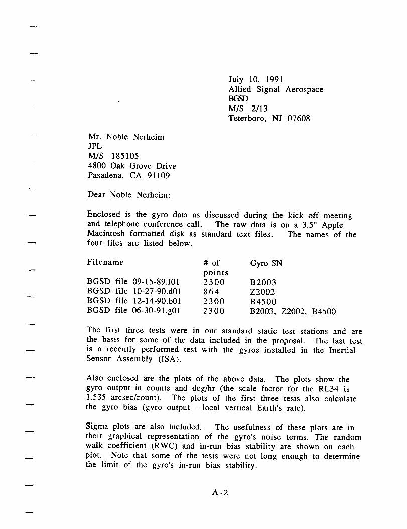
Mr. Noble NerheimJPLM/S 1851054800 Oak Grove DrivePasadena, CA 91109
Dear Noble Nerheim:
July 10, 1991Allied Signal Aerospace
M/S 2/13Teterboro, NJ 07608
Enclosed is the gyro data as discussed during the kick off meetingand telephone conference call. The raw data is on a 3.5" AppleMacintosh formatted disk as standard text files. The names of thefour files are listed below.
Filename
BGSD file 09-15-89.f01BGSD file 10-27-90.d01BGSD file 12-14-90.b01BGSD file 06-30-91.g01
# of Gyro SNpoints2300 B200386 4 Z20022300 B45002300 B2003, Z2002, B4500
The first three tests were in our standard static test stations and arethe basis for some of the data included in the proposal. The last testis a recently performed test with the gyros installed in the InertialSensor Assembly (ISA).
Also enclosed are the plots of the above data. The plots show thegyro output in counts and deg/hr (the scale factor for the RL34 is1.535 arcsec/count). The plots of the first three tests also calculatethe gyro bias (gyro output - local vertical Earth's rate).
Sigma plots are also included. The usefulness of these plots are intheir graphical representation of the gyro's noise terms. The randomwalk coefficient (RWC) and in-run bias stability are shown on eachplot. Note that some of the tests were not long enough to determinethe limit of the gyro's in-run bias stability.
A-2

We look forward to you review of this data and welcome any
comments or questions that you may have.
Sincerely,
Mark Grasso
_ / JZ- ,¢"
/..-fy, -_L_-.-_( _l_eviewed by:J J. Ficalora
CC"
Enclosed:
W. Mitchell
E. Luxford
E. Mazurkiewicz
12 data plotsone 3.5" diskette
A-3
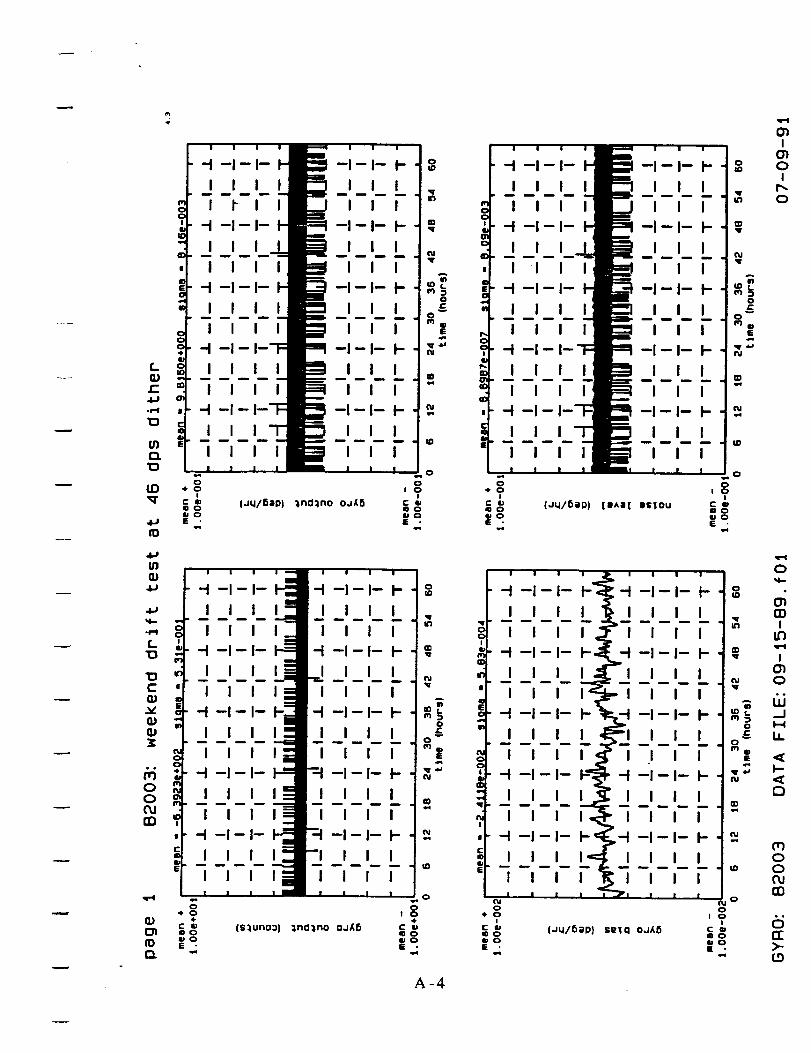
L
.I-I
-I-I
L
C
v
00(1JEl
ID01
O.
o
!C mQomoE
I I I
-I -I- I-
I I I
I I I
I I
-I-I-
I I I
I I I
A-4

L
.C
.I'I
13
O,1:3
1.0
0']Q.I
f...
"13CILl
O.l
3C
OO
0O
0,ICh
O,
(3
II
II
OO+
r_
|
x
C
E
OOO
GO
I
II
Cco
E
I IOOO÷
Oo
c_
_3
ir
V
I I
|
('aq/'6ap) ssauw0puea OJ_6 JO 60T
c_I
A-5
ooo
oo
m
000+QJ
0 00 00 04-
_I 000
I
uQJ
IDE0el
QJ
EI0In
0
0
mIO_0
Ir,.o
o
coi
_n
i
o
6J-J
h
I--
0
moo
rn
6rr)-

i"wl-
-r*'l
I/InI::)
OIn
19
16.
.el
L
CW
WW:I
OOI'UN
111OlrDn
I I I I
I I
I--I I
-I-I- I-
I I I
I I I
I I
-I-I- I-
I I I
I I I
I I
-I-I- I-
I I I
I I I
I I I
I,JU/611Pl
I I I I
I I I I
I I I I
-I- I-
I I I I
° I I I I
I I I I
-I-I-
I I I I
I I I I
I I I I
I I I I
I I I I
I I I I
c o (s_uno=)_o_oE
I I I I |
I I I I **
I I I
-I --I--I--I- ©
I I I I
I I I I
I I I I
A-6
I I
i I
I I
-I-I
I I
I I
I I
-i-!
I I
I I
I I
--!-I
, I I
I I
I I
÷ 0I
C luIDOeJol •
I I
I
I I
I-i-
I I
I I
I
I-I-
I I
I I
I
I-I-
I I
I I
I I
I I
I
I
--I"
I I
I I
I I
-I-I
I I
I
-I-I
I
I
I I
I I I I
I I I I
I I I I
--I-I-I- I-
I I I I
' I I I I
I I I I
-I -I-I- I-
I I I I
I I I I
I I I I
-I -I-I- I-
I I I I
I I I I
I I I I
0# 0
I
aDO_O
E
I I I
I I I
I I I
-4 -I-I-
I I I
I I I
I I I
-I- I-
I I I
I I I
I I I
--I-I- I-
I I I
I I I
I I I
OlOI
0
O
O0"II
0JIO,ir=l
.J
U.
I-
0
c_
fUN
rr>.

[.OJr-4-;.r-i
n
OLr)
tO
.0"l
[.13
13CQJ
Q;OJ
6JOOCUN
OJ
10O.
000-I-
I;),e-i
CUfrl
dI
x
E
000÷
0
mI
II
c
E
IOOO÷Q;OO
(3_3
to
%
I/
V
.,,,,.a
!/
//
/!
/
//
!
//
I I ! / I I !
::=1-,--
I
('Jq/'6ap) ssauwopueJ oJA6 jo 6o[
r
cfh
t6I
7/
A-7
m
w
m
OOO-l-
i QJO OO OO O-I-
Qj OOO
_rl
OOO4-Q;OOO
U3
uQ;
E°r-1
.It
Q;
r_E110
0
0
O_I
o_0
Ir_0
O13
O
Ih.CUIO
/d.J
h
I--
IZ)
_UOOC_JN
_5rr>-

L.Q.I
4-I
"0
1:1
00
4-J
-I'll
L"0
'I:)COJ
QJ
00
m
0.I
loQ.
I I I I I I I
-I --I--I-- I- '-I--I--I--I I I I I I
I I I I I I I
I I I I I I I
-I --I -- I-- --I -- I--
I I I I I I
I I I I I I I
-i --I--I-- I- -I --I--I--
I I I I I I I
I I I I I I I
A-8
I I I I I I I I
-I -I-I- -I-I- !-
I I I I I I
I I I I I I I I
-I --I--I-- I- -! --I--I- I-
I I I I I I I I
I I I I I I I I
?
O1
I
¢I
e_
I
|
÷ OI
mo
E
I I I • | I I
-I I- _
III_K_II
I I I ___l
III II
III_III
_-I--
I I
I I I | I I I J
0
(J_/Sap) seIq OJ_5
o
l
O
O
m
ID
Ot O
IC ImoeoE -
O_I0"I0I
0
0.O
0
I
ICU
6.i_II--4
LI.
l--_CO
00irl
n->-o
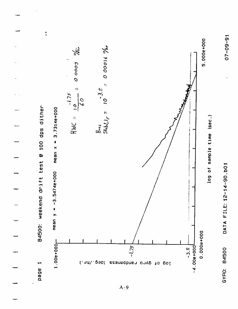
_hC)
0
_b
-$-I
L_D
C
OJ
0L_
m
I!
L oo
.C o
,,.4 _,J
if) r.
O mO_ X
C
,_ Effl
_ Ooo4-
Ig)
dI
|
Cm
E
I IOOo4-
oo
L
_5
(5
II
!
|t
I I I ! I
I
('Jql'6ep] sseuw0puej 0J_6 j0 60[
A-g
ooo+
If°OO
zI
m
m
i
00o
! ÷o o
I:_ o o_o o
! _ OOO
!
"2.u
m
E
(:1Emin
0
C_0
_r_
IO_0I
r'-0
o
o
I
i
h
,<I--
CI
00
_'.
_D

L
C
I
U313.
-r
3:QJc
r-4J._1
O3
3:13.XZ
0Lr)
03
00_JN
000Jm
O_
o.
0_D
t_
A
0
0
P3 •
E
qlr4J(v
!
00
E •
A-IO
IT)I
if)oI
0
0o_
fflI
ofrlI
ID0
..J
It.
I-
0
r_oocum
rr>-

.l.=ll
f-
i-
I
I
(n
I
Z
0IN
00
N
00
rn
QJO_tO
k_t__b
_b
ii
o "700,4- I|
cn 2:_e. C2_
d
l
X
¢-
E
OOO+
t_
MI
|
t.-
wE
I IOOO4-wOo
L
_3
6
I!
v
I I
I
('uq/'6ap] sseuwopueu ouA6 _o 6OT
A-11
OOO÷
O OO OO O÷
OoO
I
OOO.I-
OOO
u
E
a=l
Em
0
0
01I
CO0I
0
001
01I
0rr_I
_D0
_Jk-i
0
t_OOCUrn
_5IT3,-tD

0
oO
00c_JN
0o
CO
(I)C_I0r'_
A-12
I
0I
0
0
(3")I
0rrlI
o
_JI--I
i,
I--
r-I
oo
r,,J
rr>-

or'l
(3
c (3Q;
QJQ;
I It
I
o
C ÷ k../
¢- w
°r,I _
_ d
I--4X
Z cQ. m
Z E
6Oif),q.m
ai00CUN
00OJm
O_tOO.
oo0÷
o
I
ii
e.t0
E
I Iooo÷
oo
C_
0
I
IA ,-,_
I I I I I
('Jq/'6ap) ssaum0puej OJA5 Jo 6o[
A-13
I
/l
J
m
o
I°o+w
o oo oo o÷
ooo
I
ooo÷Q;ooo
Le}
LIWIn
E.0"I
Q;
nE
In
tw_
o
o
01I_D0I
0
0
,e,-i
01I
011')I
IJD0
_II,,,4
i,
0
CU00CUN
6lI>-t9

(_"0
"I0
C
v
111
I
(I)n
"1-
c
£:
0r]
"1-13.ZZ
oIN
0o
n;oo
N
oocurn
C_m
O.
A-14
01I
oI
0
0
I
o
I.tDc)
-J
U.
F-
121
0ou3
rn
rr>-
t9

.!'1
f-El
C
I
or)n>I
Q)E
i-
-e=l
olH
InZZ
m-i
0tl')
0O
00CUN
oo
O.
OOO÷
r-.
I
x
E
E
000+
0"_0
_4!
|
I-
E
IOOO+
OO
cr_
0
C_
II
I
t!
',,J
I I I
&.
ooO
II I
V
>,.
,.n ..8
(" JLI/" lap]
,
//
//
//
/
/
//
/
!oo0
A-15
u
In
E
r_E
0
0
O_I
IDO
II',-O
o
IO
IIDO
_1_-4u.
{3
oo
El
,5IT>-tO

Appendix B
Explanation of Navigation Equations
Inertial navigation systems determine change in position from an initial
reference location through double integration of acceleration measured
along three orthogonal axes. The most commonly employed method ofmeasuring acceleration is through electro-mechanical accelerometers. These
devices are configured to electrically measure the amount of force required
to restrain a proof-mass along their input axes. The electrical signal isthen converted to a digital format for computer processing of the doubleintegration to determine position.
Of course, one of the basic requirements is knowledge of the accelerometerinput axes at all times while the system is in motion so that the direction
of the change in position is determined correctly . Gyroscopes are employedin these systems for that purpose, maintaining an inertial reference for
the accelerometers following an initial alignment. Two different mechani-
zations presently are employed in practice, which are gimballed and strap-down systems. The gimballed systems locate the accelerometers on the inner
gimbal of sets of either three or four gimbals, with that inner gimbalstabilized by the gyroscopes and stabilization servos. The inner gimbal
orientation is typically maintained such that one accelerometer input axisis located along each of three navigation axes (for example, North, Eastand Vertical).
With strapdown systems, the accelerometers are nominally located alongthree orthogonal vehicle axis (i.e., roll, pitch and yaw or roll, elevationand bearing) and the gyroscopes measure the orientation of the
accelerometers (vehicle) relative to the navigation frame. The gyromeasurements are employed in this case to continuously update a coordinatetransformation matrix which takes the accelerometer measurements from the
vehicle frame to the navigation frame. It is noted that in this strapdown
case, it is necessary that the gyroscopes employed possess high bandwidthand accurate scale factor so that the accelerometer (vehicle) orientation
relative to the navigation frame is instantaneously and accurately known.The basic navigation equations in the two mechanizations are therefore asfollows:
0= X^w
B-I

m
As indicated in these equations, the gravitational field, as measured by
the accelerometer proof-masses must be compensated so as not to impact thedetermination of position.
It is also noted that the orientation of the N, E, V navigation frame,referred to as a "local level" frame of reference is dependent on the
position of the system at any given time. Maintaining this local levelframe in the navigation mode is discussed in a later paragraph.
In addition to the navigation problem, there is also the problem ofinitializing the system (determining the initial orientation of the
accelerometers). In fact, the system is capable of a self containedinitialization (initial alignment mode) if the vehicle on which it is
located remains stationary on the surface of the Earth for a few minutes.In this mode, the accelerometers are used to determine the system orien-
tation with respect to vertical through the knowledge that gravity will be
the only acceleration measured within a stationary vehicle. Similarly, thegyroscopes are used to determine the system orientation relative to East.
Since no rotation exists around that axis to be measured by the gyros thisnull condition is determined computationally (gyrocompassing). Withdefinition of the East and Vertical axes, the North axis is determined as
the third orthogonal axis in the set. It is noted that any random vibra-tion motion of the vehicle during this initialization averages to "zero"and therefore does not affect the alignment process.
To this point, the discussion has referred to a navigation frame of North,
East and Vertical. This frame of reference is, of course, rotatingrelative to the inertial frame of reference established by the gyroscopes.There is the Earth's rotation rate, and if the vehicle is moving relativeto the Earth, there is an additional rotation rate referred to as the
transport rate or navigation frame rate.
Inertial system implementations must account for these rotations. A comon
implementation is to either rotate the gimbals physically or rotate thestrapdown coordinate transformation matrix computationally at these same
magnitudes. These rotations maintain the "system" level and pointing Northand this mechanization is referred to as a North slaved, local levelimplementation.
In fact, employing this local level type of system implementation bounds
the inertial reference errors due to accelerometer biases and/or gyrodrifts due to a characteristic referred to as Schuler tuning. It is notedthat in general the limits or bound on errors applies only to the inertial
reference and cannot be extended to velocity and navigation positionerrors. In general, these errors may grow with time or time squared due
to gyro drift (particularly azimuth gyro drift) for periods up to six hoursfor velocity and twelve hours for position. It is also noted that
B-2
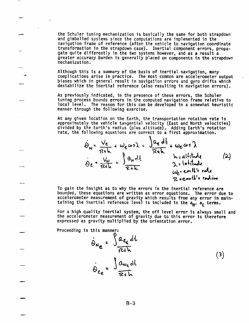
the Schuler tuning mechanization is basically the samefor both strapdownand gimballed systems since the computations are implementedin thenavigation frame of reference (after the vehicle to navigation coordinatetransformation in the strapdown case). Inertial componenterrors, propa-gate quite differently in the two systemshowever, and as a result agreater accuracy burden is generally placed on componentsin the strapdownmechanization.
Although this is a summary of the basis of inertial navigation, many
complications arise in practice. The most common are accelerometer outputbiases which in general result in navigation errors and gyro drifts which
destabilize the inertial reference (also resulting in navigation errors).
As previously indicated, in the presence of these errors, the Schuler
tuning process bounds errors in the computed navigation frame relative tolocal level. The reason for this can be developed in a somewhat heuristic
manner through the following exercise.
At any given location on the Earth, the transportation rotation rate isapproximately the vehicle tangential velocity (East and North velocities)divided by the Earth's radius (plus altitude). Adding Earth's rotation
rate, the following equations are correct to a first approximation.
V. : Ie_E
To gain the insight as to why the errors in the inertial reference arebounded, these equations are written as error equations. The error due to
accelerometer measurement of gravity which results from any error in main-
taining the inertial reference level is included in the aN, aE terms.
For a high quality inertial system, the off level error is always small andthe accelerometer measurement of gravity due to thls error is therefore
expressed as gravity multiplied by the orientation error.
Proceeding in this manner=
• 1,==
B-3

4
It has been assumed that the error in computing Earth's rate is negligible.
This is a reasonable assumption particularly early in a navigation runbefore latitude errors become significant.
{4)
The negative sign in equation (4) is a result of the fact that tilt errors
result in acceleration errors opposite in algebraic sign to the rotationrate computed by equation (2). In other words, the system in inherentlystable.
Therefore
kj.- I o.¢at
Differentiating and rearranging
,!
ONe ._ :o
_c¢ "1"¢'_+k Oe¢ :°
In fact, these equations are the equations of motion of a simple harmonicoscillator or undamped pendulum, expressed in polar coordinates, where the
length of the pendulum is equal to the Earth's radius R plus the altitude Hat the system location.
The frequency of this oscillator is:
This frequency is referred to as the Schuler frequency and the mechani-
zation is referred to as Schuler tuned. Inserting nominal values for R, Gand H in this equation, the period of oscillation computes to approximately84.4 minutes In duration.
B-4

n
d
It is also convenient to present these error equations using La Placetransforms.
They are then written:
'1,. 1,,
Examining these equations leads to a representation by two single axis
block diagrams of undamped oscillators as shown in Figure I. A completeblock diagram error representation is significantly more complicated thanFigure I (due to coupling errors that develop such as latitude error), but
these diagrams allow predicting certain errors with reasonable accuracy.For example, propagation of accelerometer bias and/or gyro drift errors for
periods up to one Schuler period are predicted with reasonable accuracy.
The results for step function errors in accelerometer bias and/or gyrodrift are shown graphically as follows. It is noted by inspection that the
tilt errors, which are the errors in computation of the inertial reference,are always bounded in this stable oscillator. It is also noted, however,
that since the oscillator is undamped, the errors remain indefinitely oncethe oscillator is disturbed.
V..,4Z'rr_Y" Sot,,,,-¢..¢. _'lve,r (_W_t'_._
o.TR (.L..-o. 1_ ,_w.A..
z.-ot,-
B-5

L__ _ _,_
./ :_) --- + 2
B-6

Development of the navigation equations is closely related to equations (I)and (2) and Figure I. In fact, the equations for latitude and longituderate are as follows:
R%-c ;L= b)
Where R is the local corrected value of Earth's radius.
The AN and AE accelerometer measurement terms are measurements in an
inertial frame of reference and therefore must be corrected for Corioliseffects to determine acceleration relative to the Earth.
In other words
Assuming a spherical Earth as a first order approximation
%-g"-
These equations operating in conjunction with the "leveling" rotations andNorth slaving rotation define a North slaved, local level inertialnavigation system.
B-7

and (2) and Figure I.rate are as follows:
Developmentof the navigation equations is closely related to equations (I)In fact, the equations for latitude and longitude
WhereR is the local corrected value of Earth's radius.
The AN and AE accelerometer measurementterms are measurementsin an
inertial frame of reference and therefore must be corrected for Corioliseffects to determine acceleration relative to the Earth.
In other words
Assuminga spherical Earth as a first order approximation
Theseequations operating in conjunction with the "leveling" rotations andNorth slaving rotation define a North slaved, local level inertialnavigation system.
B-8

w
Due to problems with navigation over a pole (convergence of longitude)
these equations are modified to develop what is referred to as a unipolar,
wander azimuth configuration. A "pole flag" is employed which changes signautomatically at the equator to prevent divergence in the navigationequations at the single pole in the mechanization. One development of thismechanization is as follows:
Modify the North slaving rotation rate as follows:
to
The plus or minus sign is selected at the equator depending on hemisphere.
In the Northern hemisphere
In the Southern hemisphere
A second definition is that longitude rate is equal to minus the wanderazimuth rate.
-- = d (!
In the Northern hemisphere
It is seen that a difference will develop in the "location" of acceler-
ometer measurement reference axes (X-Y axes) relative to the Earth's N/Eaxes.
Figure 2 illustrates this situation
B-9

kl
'_--F_
B-IO

q
Velocity and acceleration in the X-Y coordinate frame is therefore
'vy-=,-_.V_ -s,_ •VG,"
"'v,(- -5 _. V,j - _s _, V_£Differenti ating
Combining the last two equations
Substitution of equation (11) in (17) and simplifying with
Define rotation rates
(15)
_ Vw
B-11

Et: _ _,_'k: _,=v
Substituting of (19) into (18)
_J,,-A,-[}_,,,=,_,,,]v_,b-_,,,-I',1,v,,
Which are the basic unipolar navigation equations.
In order to navigate in this mechanization, a set of direction cosines (anddirection cosine rates) are developed using the terms in equation (20).
The initial value of the direction cosines are determined during the gyro-
compassing alignment and updated during vehicle motion through solution ofthe direction cosine rate equations. Latitude and longitude aredetermined from the latest values of three direction cosines.
Proceed as follows:
By definition
B-12
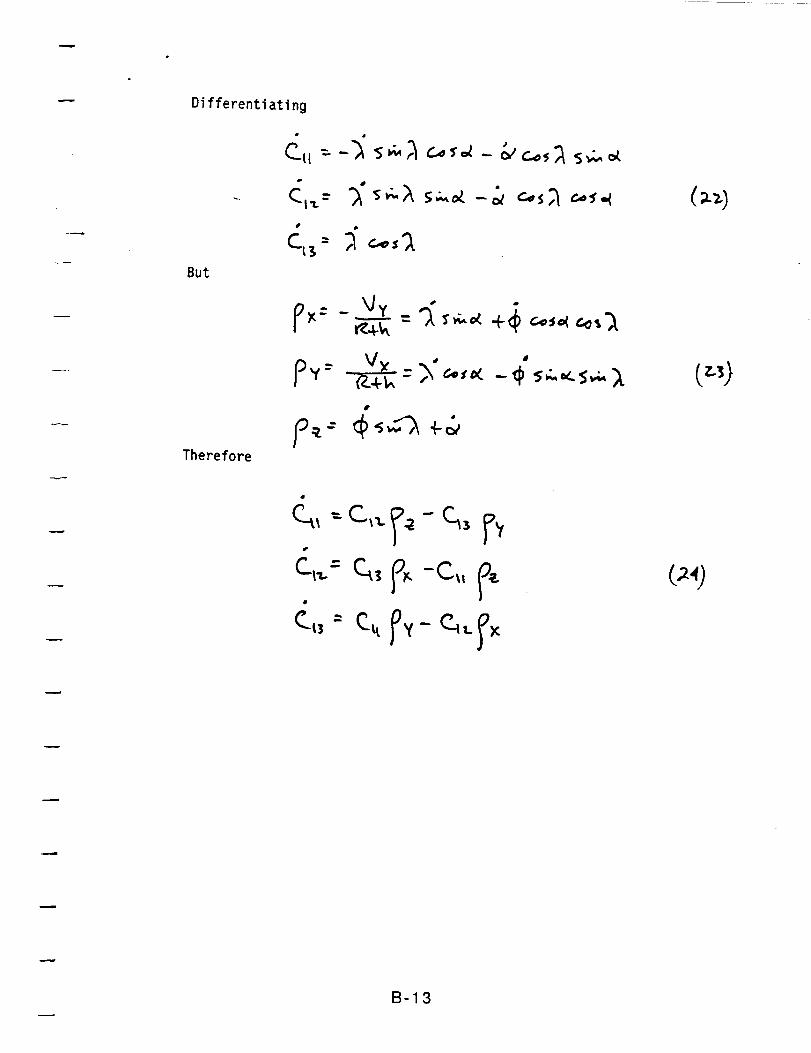
Differentiating
But
C_ -D
Therefore
B-13

These are the necessary relationships for updating the direction cosinesduring vehicle motion in order to compute values of latitude and ]ongitude.
These are computed as follows:
_c_):-_-"c,_,:_co)-_C{)-_oWhich is easily solved for longitude_ u
In addition
Which is solved for latitude
A block diagram of this unipolar mechanization is shown in Figure 3.
B-14

II | |
B-15

-- Appendix C
|
L.
eq
t-.
t..t..
sm
cm
ra_
_m
Im
Qm
L
UnCOD.
000÷
I0
t_d
I
I0E
.,-4
g_
0I
tO
I
I0
E
I
00÷
OO
000÷
O_
I
EOI4.,
In
0÷
tO
I
C
E
I
0O÷
0O
Tracking Data
i I
(0as3Jel JOJJ 3 uo_e^a[_
i I
O_
00 o° m+o
f_ tO I_
I
tO_ tO_
o¢ ca
_u " II
I I I I 0 I I I I 0O
I I I
0 O0 0+ @• 0J0 00 Q
I
0
O_
CO
L
0
E
0rl
I
00
00
I
0@
tO
I
x
C
E
0i
tO
p.)
I
E
I
00÷
0O
(3as'_Je} jojj 3 fiu_.:lu_0 d
I I I I I I I I
{3asoJe} JOdJ 3 UO!_e^@[ 3(3aS_Je) JOdJ3 u_nw[zv
oo,4-
oo
o
o+
0OO
T,0
o.
00
I
"0
(R
LoL(.LU
5
C-1
O1I
0I
010
0"10
__1I---I
I1
I--
r'l

oo ® o°,o o
II A II
m
i l l I I I I I i I I I I '
O O O÷ ÷ +
® (3asoJe) JOJJ3 u0t_,eAa[3 e = (3es3Je) JOJJ3 6ut:_ut0d" 0 0O O O
el I
=.
==
=
ee_
=o_
L
O
O÷
OIm m
(__n
|
x
L3O E
m£
W _
0m r_
m
I
C
E
o
_0
00@
00
!
I
00÷
0C
,tI
I I I I i I I I
(3as3Je} jojj 3 u0!_eAa[3
C-2
° ?
m
o=
n3
¢u
o000÷
00
00.+
u
InuL
L0f_
_ ru
5 _
_ 0"10CU
0
r, N* _J
q
o _--
= 121!

I I I I I I I I I
0,M
00÷_J00
_rI
0÷
0O0 ¢U
_Jp.
m
X
m c
LE
0
E 0I
m tO
|
CID
E
I
0÷
00
I I I I I I I I I
(3@soue) JOJJ3 UO!_I2Aa'[:I
C-3
,¢-I
_D
p,,
t'q
Od
OOOO.4-¢gOO
O
OO÷
OOO
"0
uL
L0L
0rUO10
r, /J
o LL_0
F-
I

o,,m,-i
o oo2 = o
A II
"" m (_ 010
° _m," "; II
" ' ' I , , I .,.,o " ' '
o °o °o
Q..
xI
g
° " ti,o ',,.,I _, "
_ _, ,
g g
I I ,,.,0 I I I | | | I I I I _ I,--I"-' _ o _ _§ u_
0 0 0 0
0_ (0as::)Je} JOJJ_l q:ln=tzv _' e (0asoJe] JOJJ_l UOt'_eA@[3 _E_ 0 " 0 0 F-
rO o o o or_ _ _ _" _' n
I !
C-4

|
&.
_0
@
L@LL
=i
ol
@
c_
_wemml
_W
oll
L
0Jtmr0a
O
|
_A
m
i I I I i I | _0
0 0+ +
w {3as3Je) JoJJ3 uot_eAa[3O " OQ O
I
OOO÷
CO
|
E
(3@s3Je)
L
O
WE
C-5
I
0÷
00
(_as:)Je) JOjj 3 RuT :lUTod
I a I I I I I I
{_as_Je) JoJJ3 uot3e^a[3
_nI
I',-0
I,ir-I
'I-"1
19
O'l0
0"10
_1I---I
i,
I--

oI
0
L
L ®L E
(3as3Je) JOJJ_l uo .t _,e^a[3
.¢eu
_0
oU
r=
|
(n
oo=
_D
|
I I
P3
0JC_R)CL
00÷
00
4
(3aSOJe)
0
0
O_
L
0
E
| ,,.,O
OO÷
OO
!
C-6
OOO÷
O
,4|
x
C
WE
0I
0
|
r-
E
0÷
COL_
|
C
E
0÷
O0
I
00+
00
(0as3Je)
i I
(oasoue)
I I I I I
JOJJ3 uo_ _,eAa [ 3
O I
0I
LOOJ010
._1I--I
I--
rh
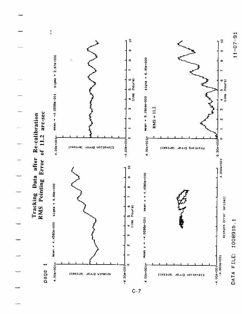
emil
o÷0J
omm (2)
=• 01
s
OOO÷,11O
G)m
l
CID
E
O
8
|
'm Iln _
"_'_. i l J , e l , , _o
÷
('_aS;),J_) dOJJ::l u0_leAaI:l• o
o
_rI
I
o
(1.) +¢g01 o
ro or-_
I I I I
(3;)S3JR) JOJJ_l u_.rlWT ZV
r_
L
0
E
m
OO÷
OO
I
0-7
OO
O4-
O
|
x
Ca3
E
0I
0301_D0
I
|
C
E
I
00@
00
II
JOJJ3 GuT_uTOd
, i ! I I I
JOJ,J3 uot _,e^a[3
0
O_
OO
(_
0
m£
r_
0000
e,00
O
+
OO
(.O(_LUJ
5
O
;7OO
I
O1I
p_OI
r-1
01
0o
._1
LL
I--
0

=
em
_. Q0
elml
_a
_k
I_
_r_
=im_0_
= =ommm im
==
E_
EL
00,04-
r'-
|
E
m
00I
0
IZl
I
B
¢-I0
E
l I i i i I I I
0÷
m (3aG3JR} JOJJ3 uo_'_e^aI3o
8
|
m
|
I I I I I I I
O+
w {_as3Je) JOJJ_ q_nwtzVoo
o
0_
r_
L30
1=
,,,.. O
OO÷
OO
I
O
L3O
I11E
m
I..,O
OO÷al
OQ
I
C-8
0O,0.,I-
QD
|
E
000÷
_r_Unj C_
II|
I I
O÷
OO
OOO÷
OLr)
kq
rd|
r-
E
OOI
Ot_
i
|
Q3E
I I
O4-Q3OO
I I I I
(:}@S_Je) JOJJ3 6uT_uIOd
i
i o I I
ooo
oo
I I I a I I I I
( 3_'IS 3JI2) JO J J=l UO! '_I2Aa [ _
m
_r
oo-i.
(3(3
o
_r
m01uLI0
(.0(_
g cu
s
_ O0Oo
_ .J_ t-.-4
o I--.
o <IZ" 1:3I
01I
p.0I


emme |
l
r,.
_..=
°-,,
(D
rOCl
000+&lIDO_
I
IDE01
000÷
0m
fu
|
r-
E
I
04-
00
I I I
(0as_Je)
I i i I !
JOJJ_ uo_e^at3
0÷
00
0
a3
P.
L
0
II1E
Orl
,,,_0
00÷m_00
I
0
m
LD0
E
C-I0
0
O_
I I I I I I I I
(:)_s:)Je} u0JJ:l u0_e^,_[:l
L
0
E
It_o
I,e-.l
cu
.0
0'10'100
,',i_1
14_
I--
0

C-11


Gyro
Appendix D
Data over Temperature and Thermal Model
STATIC TEMPERATURE DATA
Gyro: Z2002Data file: 06-07-90.b01
chamber temp. output random walk gyro T. T. dev.(deg.C) (deg/hr) (deg/rt-h0 (deg.C) (deg.C)
....................................................
25 9.8246 0.0003 26.24 0.2045 9.8235 0.0011 44.59 0.1970 9.8233 0.0008 66.88 0.1945 9.8255 0.0006 42.12 0.3125 9.8238 0.0007 27.08 0.135 9.8239 0.0005 8.21 0.20
-15 9.8230 0.0008 -10.30 0.30-35 9.8238 0.0004 -26.70 1.61-55 9.8230 0.0011 -47.87 0.41-35 9.8240 0.0008 -29.73 0.41
delta T dT dev.
(deg.C) (deg.C)
-0.18 0.01-0.11 0.01-0.06 0.01-0.66 0.02-0.09 0.00
-0.16 0.01-0.23 0.01-0.24 0.01-0.33 0.01-0.32 0.01
summarypeak to peak variation of 25 degree points = 0.0008 (deglhr)average random walk = 0.0007 (deg/rt-h0
thermal model
output = bias + local vertical earth rate + k0*dt +kl*T + k2*T"2 + k3*T"3 + k4*T"4
where T = gyro temperature - 25
bias = 2.3160e-001 (deg/hr),k0 = -5.000e-003 (deg/hr/deg.C)kl = 4.278e-003 (deg/hr/deg.C)k2 = 2.713e-005 (deg/hr/deg.C"2)k3 = 7.51 le-008 (deg/hr/deg.C"3)k4 = 7.643e-011 (deg/hr/deg.C"4)
bias repeatability = 0.0005 (deg/hr 1 sigma)
D-1

(/)
OJ
-r"l
.r-I
.oro
ii]
oJc1OJC_
U)fO
-f"l
.C)
fO1::)
LF)
00CUN
a;
Q
II
x
°
ii
!
I!
I!
!I I I
[Jq/6ap] lndln0
u
E
m
m
m
m
c_
m
= '3",
0.Q
0O_I
r,.oI
LC)0
._II-4
h
l--
C_
0o
N
OZ
I
0I

>,
.r-I
r-4
.r=i
roIDO.
L
.t-i
>,I0I:)
IfJ
00C_JN
01fO(:I
I I I
I I I
I I I
7-i--I-
I I I
I I I
I I I
-I- I-
I I
I I
I I
-I-I-
I I
I I
I I
I
I
I
_ _ r
I
I
I
-I- - I-
I I
I I
I I
--I--I--I-
I I I
I I I
I I I
I I
I I
I I
- -I-I-
I
I
I
7-I--
I I
I I
I I
-I -I- I-
I I I
I I I
I I I
I
I
I
I-
I
I
I
I"
I
I
I
I-
I
I
I
I
I
I
rI
I
I
r-
I
I
I
I
I
I
OI O
CmO
E •
inL
E
I I I I
I I I
I I I
7 -I- I-
I I I
I I I I
I I I I
7 -I- I-
I I I I
I I I I
I I I I
-I -I- I-
I I I
I I I I
I I I I
I
I
I I
7--I
I
I
I
-- --j
I
I
I
I
I
I
I
I I
-I- I-
I I
I I
I I
-I-I-
I
I I
I I
(_q/Sap) [e^et astou
I I
I I
I,
I
I
I
I I
I I
I I
-I-I-
I I
I I I
--jm
I
I
I
-I - I-
I I
I I
I I
I
I
I
I-
I
I
I
r-
I
I
I
I-
I
I
I
L
01IDO0I
0.0
001I
0ILO0
_J
I---
121
CU00CUN
n->-
D-3
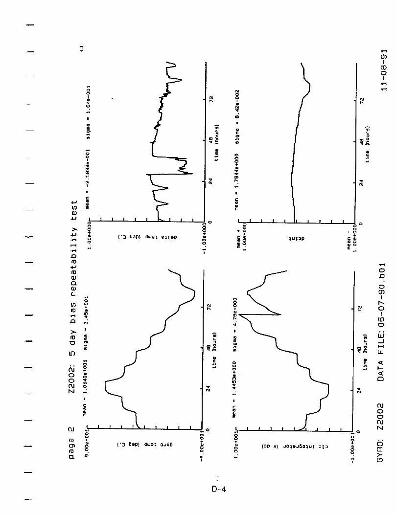
0I
a;_rID
|
E
m
r,0I
|
I I I I I I
.IJ-r"I
.e-I
.0
(3.)r'_
(..
+
I,rl• r-I '_r
n f,1I
m
i.n
o ®00 '_njN ..,
I
C
QE
I
0
{'3 6ap) _w_l e_laD
I I II_ I I I I
['0 6_p} 0wa_ oJ_6
I0004-tl00
P_
e3
¢.
tlE.eq
_rt_
o
elL
co o
E
.hi
,.,o
o0+
00
I
0oI
t'U
|
OE
M
000+
_r
_rO_
,eq
|
E
!
00
+ 0+
C_0_0E •
I I I
t
I I I I l I
+oGI
00+
OO
(%1r_
mL
E
4J
(u
000
I C)+
C
0E •
L
00+¢uC)C)
IE
O_I
O30I
'el
,e"l
0
0O)Ih.0I
0
..J
LI.
I--
121
00OJ
r_
D-4

D-5

STATIC TEMPERATURE DATA
Gyro: B2003Data file: 09-29-89.a01
chamber temp. output random walk gyro T. T. dev.(deg.C) (deg/hr) (deg/rt-hr) (deg.C) (deg.C)
25 9.7887 0.0005 26.04 0.0945 9.7872 0.0006 44.45 0.2170 9.7849 0.0005 67.80 0.2145 9.7877 0.0005 45.37 0.2325 9.7896 0.0005 26.82 0.175 9.7897 0.0006 7.94 0.15
-15 9.7923 0.0006 -10.74 0.07- -35 9.7933 0.0008 -28.83 0.41
-55 9.7960 0.0006 -47.15 0.38-35 9.7939 0.0008 -30.44 0.37-15 9.7924 0.0005 -11.67 0.30
5 9.7906 0.0006 7.22 0.2625 9.7899 0.0006 25.88 0.28
delta T dT dev.
(deg.C) (deg.C)
0.00 0.00
0.00 0.00-0.00 0.000.00 0.000.00 0.00
0.00 0.000.00 0.000.01 0.01
-0.00 0.000.00 0.000.00 0.00
0.01 0.000.01 0.00
summarypeak to peak variation of 25 degree points = 0.0012 (deg/hr)average random walk = 0.0006 (deg/rt-hr)
thermal model
output = bias + local vertical earth rate + k0*dt +kl *T + k2*T"2 + k3*T*3 + k4*T"4
where T = gyro temperature - 25
bias =-1.3823e-001 (deg/hr),k0 = 0.000e+000 (deg/hr/deg.C)
1_ = -8.686e-O04 (deg/hr/deg.C)-2.561e-006 (deg/hr/deg.C"2)k3 -4.281e-010 (deg/hr/deg.CA3)k4 6.516e-012 (deg/hr/deg.C"4)
bias repeatability = 0.0004 (deg/hr 1 sigma)
D-6
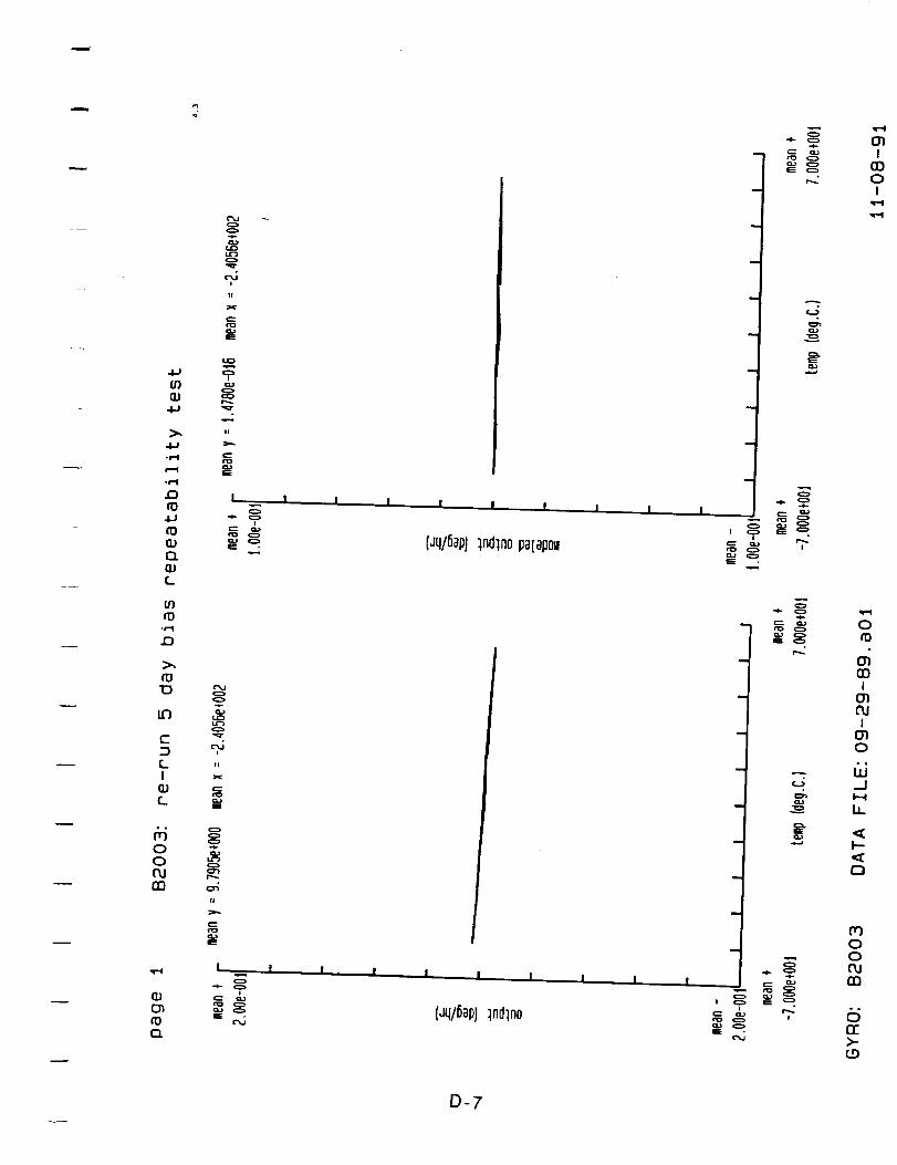
O')
4J
>,,4J
.el
.0
4J
QJO.
(..
0ofO
.j-g
.0
01=)
c
I
oo
m
r0ci
o
II
ii
r,-
E
o
tl
o
II
(Jq/fiap}:lndln0pa[ap0=
[Jq/6ap)lndln0
m
o.)
-- ._
- _
o
m
m
o
m _
m
, ,_ _.N _
ed
O1I
110oI
o
I@1
I0"1o
_J
,_cI--
0
00cug]
n->-
D-7

4J
4J
.1-1
r_
_J
ELOJC.
L_
-PI
17
110"13
Ln
C
{..I
OJC_
• °
00{Xlm
01fO{:I
|
I
I
7 -I- - !-"
I I I
I I I
glL
0
I I I I
I I I I
_ 7 -I-r--t--
I I I I
I I I I
-1 --I--I-- L
I
MQ
4.
C
117
!
I
I
M
O+ O
÷
(s:luno_)go• OE -
I I I I
I I I !
-I --I--I-- r
I I I I
I I I I
-i _1_1_ i_
I I I
I I I
I I I
I I I
I I I
I I I
- -I-I- r
I I I
I I I
_nd_no oJX6
0I 0
+
IDO
E
ID01
01L
0
O
D-8
I I I
I i I
-I -i-I-
I I I
I I I
-I -I- I-
I I
I
I
I
I
I
_j _
I I
I I
I
I
"I
I
I
J
I
I
I
I
I
I
7
I
I
I I I
_1 I I I
-i-I- I-
I I I
I I I
-I-I- I-
i
I
I
I
'1 I
{JqlSaP) [aAaT asTou
I I I I I
I I I I I
-I - "I -I - I-
I I I I I
I I I I I
I I I
I I I
I I I
I I .II I
I I I
--I- !- T -I
I I I I
I I I
I I
I I
I I
I I
I I
I
I I
OiI
OI
0110
_0I01CU
I010
_1I.--'4
LI.
I--
121
00Odm
IT">-

00
I
M
I
E
m
D-9

.IJ
(1;
.lJ-Ill
r'--I
,r=1
Z];13
n3oJCloJ
cofo-r'1
Z]
110"D
Ln
C
LI
L
00C'UO3
0
Ill ,¢" m
0'1 mofO cuoE *
Q.
(dwvw}
I " I I
_uadJn3 le_o_
00CUm
_5rr)-CO
D-IO

STATIC TEMPERATURE DATA
Gyro: B4500Data file: 03-30-90.a01
chamber temp. output random walk gyro T. T. dev. delta T dT dev.(deg.C) (deg/hr-) (deg/rt-hr) (deg.C) (deg.C) (deg.C)(deg.C)
25 9.8165 0.0004 26.39 0.04 -0.48 0.0045 9.8169 0.0005 43.90 0.22 -0.48 0.0070 9.8188 0.0005 66.64 0.16 -0.54 0.0045 9.8165 0.0005 44.72 0.45 -0.46 0.0025 9.8154 0.0005 26.39 0.33 -0.44 0.005 9.8133 0.0004 8.00 0.19 -0.44 0.00
-15 9.8118 0.0007 -10.71 0.20 -0.46 0.00-35 9.8110 0.0006 -29.20 0.29 -0.50 0.01-55 9.8110 0.0004 -48.14 0.40 -0.48 0.01-35 9.8110 0.0005 -30.08 0.31 -0.50 0.02-15 9.8118 0.0005 -11.40 0.32 -0.51 0.00
5 9.8138 0.0005 7.27 0.27 -0.53 0.01
summarypeak to peak variation of 25 degree points = 0.0011 (deg/hr)average random walk = 0.13005 (deg/rt-h0
thermal model
output = bias + local vertical earth rate + k0*dt +kl*T + k2*TA2 + k.3*T"3 + k4*T*4
where T = gyro temperature - 25
bias = 2.0200e-001 (deg/hr),k0 = -5.000e-003 (deg/hr/deg.C)
kl = 4.249e-003 (deg/hr/deg.C)k2 3.024e-005 (deg/hr/deg.C 2)k3 = 9.561e-008 (deg/hr/deg.C^3)k4 = 1.113e-010 (deg/hr/deg.C^4)
bias repeatability = 0.0003 (deg/hr 1 sigma)
D-11

4-1
In0J
4.1
>,
4-;
.r-g
.O
(1)CL
£.
43
OLn_Trn
03C_COC_
I!
==¢
t,--
E
o,3m
ii
i!
[Jq/Oap} lndln0 pa[apc_
q
l
m
m
m
m
ro
!
===
II
i
m
_=_ , _ =_
cnI
130OI
0
00")
I
0p')I
(.r)0
_JI,--4
Lu
0
00i._
m
(5rr
D-12

4.1
Q,I4.1
4_.e'l
r-=l
.OcO
Q.
(,
I0
.O
0Lr)
m
oJ
r0O.
;;/;;I I I I
I I I__1 I !-I--I I-I-
I I_ I II I I: I I I
I
I
I
7
I
I
-I - I-
I I
I I
I I
I I I
I I
I I I
-I - I-
I I I
I I
I I I
I I I
7 -I- I-
I I I
I I I
-I -I - I-
I
I I I
I I I
I I I
I I I
I I I
7 -a-l-
I I I
I I I
D-13
I I
I I
7-I-
I I
I I
-I-I-
I I
I
I-
I
I
I-
I
I
I I
I I
I
I I'.
I-
I
I
I I
I
-I - I-
I I
I I
-I - I-
I I
I I
I I I
I I
I
I
I
I
I I I
I I I I
7-1-1- I'- T
I I I I I
I I I I I
-I-1-1-1-4-
I I I I
I I I I
I I I I I
I I I I
I I I I
I I I I
-I-i I- T 7-1-I I I I I I
I I I I I I
I I
I
I
I
I
I
I-
01I
0I
0
001
I
0t,,r1
I
mo
._1I--t
I---
IZ)
0
m
rr

4J03
4J
4J
.(D
4-J
ClQJ
L
CO.f-I
.IS)
0U__T
QJC_
Q
QQi
0
_r
I
10Eot
IN0oim
° 4t_
ID
0÷ 0
IE=DO_0E •
|,-i
,i=
L
@"
-- I I I I
(dwpw) _,uaJjn:) e:l[al:)
00I¢gn.I
I
E
m
t
(D
mL"10r"
=..=
mr
m o
oI 0
IC#DO_0E
m
0
£
==
Og
=r
o=
I
4J
_r¢u
0I 0
IC
0
O1I
CO0I
0tO
0
I0
I
0
_J
b.
0
00
m
IT
LD
D-14

Appendix E
Differential E.quation Gyro Model
The following differential equation describes a model for RLG angleerror:
e= EGB + EGBw +EGBsF + EGBI + QN + EGN
where:
EGB is the error in fixed gyro bias.
as a random, initial bias.
It is modelled
EGBw is the gyro bias warm-up error, and is
modelled as an exponentially decaying uncertainty
in gyro bias. The uncertainty is reduced with timeuntil a lower limit is reached after which it is
modelled as a fixed random bias.
e.g.
if E(EGBw) 2 >_ (_2 limit
then model: =-dt
EGBw
'17
else model: ' ' _" O
dt
E-1

EGBsF is an error in gyro rate produced by an error
in gyro scale factor.
eGBsr: = ESF *
a(sF)I_ -0
dt
where:
is the sensed gyro rate, and
E SF is the error in gyro scale factor. This error is
modelled as an initial random scale factor error.
The next three terms are the major sources of noise
that exist in the RL-34 gyro and are related to those
variances typically used in gyro testing to
compute/model the noise equivalent rate(NER).
EGBI is the random bias error. This error source is
used to model gyro bias instability. This is
modelled as a first order Markov process:
d(EGBI) £GBI- - _ + nbm
d t '_brn
where nbm = w(t)* "_/2*(_'bm 2
"_bm
for long term stability, a random ramp model isused:
d(EGBI)-0_
dt
d(0_)-O ; _ = Random Ramp
dt
E-2

QN is the quantization noise due to gyro output
angle quantization. It is modelled as an integral of
gyro quantization(producing gyro angle error) by a
white noise process with variance bounded(uniform
distribution).
EGN is the gyro random walk in angle, which has a
white rate noise distribution in power spectral
density.
E-3

Appendix F
Description of Raw Data Records
Four data files are included on a 3.5" Macintosh formatted disk
as standard test files. The names of the four files are listed below:
Filename
BGSD file 090991a.dat
BGSD file 100991b.dat
BGSD file 101191f.dat
BGSD file 700Hz
Description
Example of an initialization test
Example of two tracking tests
Example of an acquisition test
Example of 700 Hz data
The first two files contain gyro X, Y and Z outputs in 'deg/hr',
accelerometer outputs in 'Gs', system attitude (heading, roll, and
pitch) in 'mils', and alignment/navigation time in 'seconds'. The last
file only contains the system attitude and alignment/navigation time.
The alignment/navigation time is a system variable that is used to
either show the time left in alignment mode or the time in navigation
mode. The 700 Hz data file only contains X,Y and Z gyro counts.
For example, Figure F-I shows the first 30 points of BGSD file
090991a.dat. During this test, multiple 15 minute alignments were
performed. The alignment/navigation time starts at 900 (15 minutes
= 900 sec) and counts down to zero, then counts up until commanded
into align mode again (300 seconds later). Note, the data acquisition
was performed asynchronous to the alignment/navigation time. The
heading data recorded in table III (pg 24) of the report is the last
data point while still in align mode. For example, the first value and
second points in table III corresponds to data point 10 and 22.
respectively.
Figure F-II shows the first 30 points of file BGSD file
100991b.dat. This datafile contains two tracking tests. Data points
3-11 show the alignment data. Data point 13 shows the acquisition
data (20 azimuth and 60 deg elevation). Data points 14 though 388
show the 10 hrs of tracking data. After the 10 hrs of tracking was
complete, the system was re-initialized and a second tracking test
was performed. Data points 389 to 397 represent the second
alignment and points 398 775 represent the second tracking test.
BGSD file 101191F. DAT contains the raw data records of a
compound angle acquisition test (azimuth table rotation rate at 0.2
deg/sec from 350 deg azimuth and 0 deg elevation to 330 deg
F-1
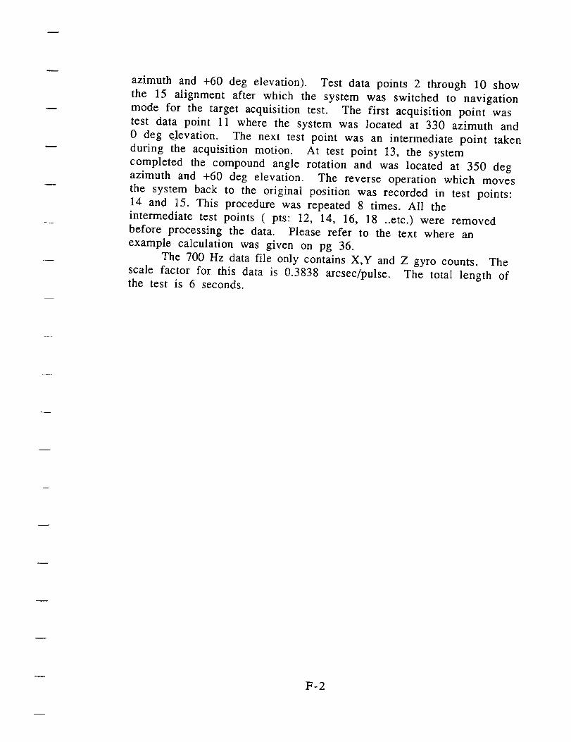
azimuth and +60 deg elevation). Test data points 2 through 10 showthe 15 alignment after which the system was switched to navigationmode for the target acquisition test. The first acquisition point wastest data point 11 where the system was located at 330 azimuth and0 deg elevation. The next test point was an intermediate point takenduring the acquisition motion. At test point 13, the systemcompleted the compound angle rotation and was located at 350 degazimuth and +60 deg elevation. The reverse operation which movesthe system back to the original position was recorded in test points:14 and 15. This procedure was repeated 8 times. All theintermediate test points ( pts: 12, 14, 16, 18 ..etc.) were removedbefore processing the data. Please refer to the text where anexample calculation was given on pg 36.
The 700 Hz data file only contains X,¥ and Z gyro counts. Thescale factor for this data is 0.3838 arcsec/pulse. The total length ofthe test is 6 seconds.
F-2

x_LU
Qo_jQ
C_
r_n
J_

Ux
--- LU
.0
00
Q
03
GO
Recommended


![Vertical Openings Inspection System [VOIS] Development and ...€¦ · • Active gyro stabilisation system and platform decoupled slip ring assembly • Laser scanning using OEM](https://img.pdfslide.us/doc/110x75/5f170845b5aad850ac4f5674/vertical-openings-inspection-system-vois-development-and-a-active-gyro-stabilisation.jpg)