Review of Marketing ScienceWorking Papers
Volume , Issue Working Paper
The Market for Television Advertising:
Model and Evidence
Robert Kieschnick B. D. McCulloughUniversity of Texas at Dallas Drexel University
Steven S. WildmanMichigan State University
Review of Marketing Science Working Papers is produced by The Berkeley Electronic Press(bepress). http://www.bepress.com/roms
Copyright c©2002 by the authors.
The author retains all rights to this working paper.
The market for television advertising: model and evidence*†
Steven S. Wildman Department of Telecommunication
Quello Center for Telecommunication Management and Law Michigan State University
409 Communication Arts & Sciences Building East Lansing, MI 48824-1212
B.D. McCullough
Department of Decision Sciences Academic Building, Room 230
Drexel University Philadelphia, PA 19104
Robert Kieschnick School of Management
University of Texas at Dallas P.O. Box 830688, JO5.1
Richardson, Texas 75083-0688 [email protected]
* The authors wish to thank G. Biglaiser, J. Herman, J. Prisbrey, F.W. McElroy, A. Prasad, R. Ramanathan, M. Riordan, J. Rogers, H. D. Vinod, and D. Webbink for helpful comments on prior drafts. Further comments are welcomed as this is a work-in-progress.
† The order of the authors� names was randomly assigned.
1Kieschnick et al.: The Market for Television Advertising
Produced by The Berkeley Electronic Press, 2011

Abstract
We provide a model of television advertising based on an explicit characterization of an advertisement�s contribution to an advertiser�s profits that suggests that each program faces a downward sloping demand for its ad time. Hence Fournier and Martin�s (1983) �law of one price� does not hold in our model. We study these contrasting arguments about television advertising by examining the pricing of broadcast network advertising. In conducting this empirical examination we encounter and solve a severe multicollinearity problem. We conclude that the evidence supports the advertising model presented in this paper and demonstrates segmentation between cable and broadcast viewers in the national television advertising market. key words: broadcast, cable, market segmentation, multicollinearity
2 Review of Marketing Science Working Papers Vol. 1 [2002], No. 2, Working Paper #5
http://www.bepress.com/roms/vol1/iss2/paper5
1. Introduction
Advertising plays a critical role in the funding of media in the United States, even
of new media such as the Internet. Despite this role, economists have devoted little
attention to the pricing of advertising. For example, economic models of competition
among broadcasters and networks that rely, at least in part, on advertising revenues have
traditionally employed fairly simple characterizations of advertisers� demand for
advertising time. Most common has been the assumption, dating back at least to Steiner
(1952), that advertisers are willing to pay a constant amount per viewer delivered, i.e.,
that suppliers of advertising confront an infinitely elastic demand curve. The common
justification for this assumption is that a variety of media compete vigorously to supply
advertisers with access to potential customers, and this competition sets the competitive
price for access to viewers that broadcasters take as a given in their competition with
each other (Chaudhri, 1998). This is what is called the �law of one price� in Fournier and
Martin�s (1983) study of television advertising.
Alternatively, and more rarely, a downward sloping inverse demand function with
the amount of ad time (or space for print media) may be postulated. But this is more
common for models of media monopolists (see, e.g., Blair and Romano, 1993.) For the
analysis presented in this paper, we begin by explicitly modeling the demand for ad time
on television programs as a function of a TV commercial�s contribution to advertiser
profits. We show that, for a model of competition in the sale of TV ad time based on this
foundation, there is no market-determined price for ad time that sellers must take as
exogenously given. Rather, each program sees the demand for its commercial time as
downward sloping, regardless of its competitive circumstances. So the �law of one
price� does not hold in this market. Furthermore, different viewers in a program�s
audience may be sold at different implicit prices.
To present our arguments and the evidence on them, we organize this paper as
follows. Section 2 presents our model. Section 3 presents a test of one of the model�s
implications. Section 4 concludes the paper.
3Kieschnick et al.: The Market for Television Advertising
Produced by The Berkeley Electronic Press, 2011

2. The model
2.1 The basic model
We consider two types of programs: programs distributed by over-the-air or
broadcast services and programs that are distributed on a subscription basis by non-
broadcast services, e.g., cable operators and direct broadcast satellite services (DBS), like
DirecTV and the Dish Network. We will refer to the two types of programs as broadcast
programs and �cable� programs. For our purposes, the critical distinction between the
two types of programs is that cable programs are received and viewed only by subscribers
to cable and satellite services, while broadcast programs are received and viewed by
cable and satellite subscribers (as retransmitted signals) and by viewers who rely solely
on rooftop and set top antennas for receipt of the over-the-air signals broadcast by
television stations.
To simplify the analysis and notation, we assume a single representative
advertiser, which plays a role similar to the representative consumer employed in many
monopolistic competition models.1 The advertiser sells a single product, produces a TV
commercial to promote it, and purchases ad time on broadcast and cable programs to air
the commercial. We assume: that only consumers who know about the advertiser�s
product will buy it; that the probability of knowing of the product�s existence in the
absence of advertising is less than unity; that exposure to an ad for a product makes a
consumer aware of the product only if the consumer notices the ad within a program that
carries it; and that the full effect of the ad on a consumer�s purchase probability is
realized the first time the consumer notices it.2 In particular, we allow for the possibility
that a viewer may watch a program but fail to notice the advertiser�s ad during a
commercial break. The advertiser can increase the probability viewers will notice its ad in
a program by increasing the number of times the ad is aired during the program.
Viewers watch television for a period (say, a week), which we will call the
viewing period, during which they have the opportunity to watch each of the programs
1 Spence (1976) and Dixit and Stiglitz (1977) are prominent examples. 2 We can relax our exposure assumption to allow a consumer�s purchase probability to be a concave function of the number of ad exposures, as typically in the marketing literature, e.g., Lilien, Kotler, and Moorthy (1992). However, such a relaxation complicates our analysis without changing its basic conclusion regarding the nature of the ad time demand function faced by program owners.
4 Review of Marketing Science Working Papers Vol. 1 [2002], No. 2, Working Paper #5
http://www.bepress.com/roms/vol1/iss2/paper5

offered by the broadcast and cable services once. The advertiser may purchase
commercial time on any or all of these programs. At the end of the viewing period is a
shopping day during which a viewer either may or may not purchase the advertiser�s
product. We assume that noticing the advertiser�s commercial makes the same
contribution to the purchase probability for all viewers.
The model makes use of the following terms:
m ≡ the number of cable programs. Subscripts h, i, and j will be employed to
identify individual cable programs.
n ≡ the number of broadcast programs. Individual broadcast programs will be
identified with the subscripts d, e, f, and g.
ak ≡ the number of units of advertising time that the advertiser purchases from
program k, where k may be either a cable program or a broadcast program,
and a unit of ad time is the time required to play the advertiser�s
commercial once.
r(ak) ≡ the probability that a consumer watching program k will see and
remember the ad for the advertiser�s product on program k. We assume
r’> 0, r”< 0, and r(0) = 0.
pik ≡ the probability that a subscription viewer who watches cable program i
will also watch program k, where k may be either a broadcast program or a
cable program.
pgk ≡ the probability that a subscription viewer who watches broadcast program
g will also watch program k.
tgk ≡ the probability that a broadcast-only viewer who watches broadcast
program g will also watch program k. (Obviously, tgk=0 if k is a cable
program.)
5Kieschnick et al.: The Market for Television Advertising
Produced by The Berkeley Electronic Press, 2011
Vg ≡ the number of broadcast-only viewers in the audience for broadcast
program g.
Wg ≡ the number of subscription viewers in the audience for broadcast program
g.
Wi ≡ the number of viewers in the audience for cable program i.
Because the full contribution of an ad to a consumer�s likelihood of purchase is
accomplished with a single noticed exposure, the value of ads on any given program is
the contribution they make to the likelihood that a consumer will notice the ad at least
once during the viewing period on any of the programs on which the ad airs. Thus,
critical to our analysis are: Si, the probability that a viewer of cable program i will
remember only an ad on program i; Bf , the probability that a broadcast-only viewer of
broadcast program f will remember only an ad on program f; and Sf, the probability that a
cable viewer in the audience for broadcast program f will remember only an ad for the
product seen on program f. Given the above definitions:
Si = (1− pigr(ag))g=1
n∏probability viewer does notnotice ad on anyof the nbroadcast programs
1 2 4 4 4 3 4 4 4 • 1− pij r(aj )( )j ≠i∏
probability viewer doesnotnotice ad on any of the otherm −1 cable programs
1 2 4 4 4 3 4 4 4 r ai( )
probabilityviewer noticesad on programi
1 2 4 3 4 ,
Bf = (1− tfg r(ag ))r(afg ≠ f∏ ),
and
Sf = (1− pfgg ≠ f∏ r(ag)) • (1− pfjr(aj ))j =1
m∏ r(af ).
Because it provides a simpler starting point while providing a useful comparative
benchmark, we begin by examining the nature of competition among broadcast programs
selling ad time in a hypothetical television market in which all programs are delivered by
television stations over the air. This, of course, is a description of the market for
television ad time before cable emerged as a major supplier of television audiences to
advertisers in the 1980s. In modeling the competition in ad time, we take as givens the
6 Review of Marketing Science Working Papers Vol. 1 [2002], No. 2, Working Paper #5
http://www.bepress.com/roms/vol1/iss2/paper5
probabilities for each show that its viewers will also watch each of the other shows. This
is not meant to imply that factors such as production and marketing budgets that may
influence viewers� choices among programs are not strategic variables�only that
decisions on such variables precede the delivery of programs to viewers. That is, we
assume that competition in the sale of ad time is competition in the sale of the audiences
actually generated.3
Consider first the advertiser�s decision regarding how much ad time to purchase
on broadcast program f, taking for the moment the amounts of time purchased on other
programs as givens. (We show later that the equilibrium amount of time an advertiser
purchases on one program is not influenced by the amount of time purchased on other
programs.) For a representative viewer in f’s audience, the advertiser must consider two
consequences of a small increase in the number of units of ad time purchased from f.
First, the purchase of additional ad time on f increases the probability that the viewer will
notice the commercial at least once during the program, which increases the likelihood
that the advertiser�s ad campaign in aggregate will have made this viewer aware of its
product. At the same time, however, the increased likelihood that the viewer will notice
the commercial on program f reduces the contributions that the advertiser�s ads on other
programs make to the likelihood that the viewer will become aware of its product. The
net of these two effects on the likelihood that the viewer will notice the ad at least once
on one of the television programs he or she watches, multiplied by the effect of noticing
an ad on the likelihood of purchase times the advertiser�s profit margin on its product, is
the value of the marginal unit of ad time on program f to the advertiser.
These considerations are reflected in the formal statement of the advertiser�s first
order condition given by equation (1), where γf is the per unit price for ad time charged
by program f ; w and c, respectively, are the price and marginal cost of the good sold by
the advertiser (both taken as constants); q is the number of units of the good purchased by
3 Note that we also assume that differences in viewers� likelihoods of viewing different networks are not influenced by the amount of advertising time carried on the programs. This is a standard assumption in media economics literature; but if television ads are considered a bad by viewers, then the probability that a representative viewer chooses to watch any specific program should vary inversely with the amount of ad time sold by the program. See Wildman and Owen (1985), Wildman and Cameron (1989), Owen and Wildman (1992, chapter 4), and Wildman (1998), for analyses that consider this issue more explicitly.
7Kieschnick et al.: The Market for Television Advertising
Produced by The Berkeley Electronic Press, 2011
a consumer who decides to buy; and ∆ is the contribution that noticing the ad makes to a
consumer�s purchase probability.
(w − c)q∆ Vf
∂Bf
∂af+ Vg
∂Bg
∂afg≠ f∑
− γ f = 0. (1)
Expanding the expression in square brackets in (1), we have:
(w − c)q∆ ′ r (af ) Vfg≠ f∏ (1− t fgr(ag )) − Vg (1− tge (r(ae ))r(ag ) tgf
e≠ f ,g∏
g≠ f∑
−γ f = 0. (1´)
The first term within the square brackets is the probability that a viewer in the
audience for program f will not notice the commercial on any other program during the
viewing period. Multiplied by r´(af ), it gives the marginal effect of an increase in af on
the probability that this viewer will not notice the commercial on any other program and
will notice it on program f. The quantity r´(af) times the second term in the square
brackets gives the sum of the effects of a marginal increase in af on the probabilities that
the ad will be noticed on each of the other programs alone. Designate the first term in
square brackets in (1´) by Af and the second by Bf. The difference Af -Bf must be positive
if program f finds it profitable to sell ad time.
We assume competition among programs to be Cournot in ad time, so the owner
of program f takes the amount of ad time sold by other programs as givens in setting af to
maximize Rf, its revenue from ad time sales, where Rf = af γf. Program f �s first order
condition is:
af
∂γ f
∂af
+ γ f = 0. (2)
Solving (1) and (2) simultaneously, we get (3), which implicitly determines af∗ ,
the profit maximizing value of af for program f.
af∗ = −
(w − c)q∆ ′ r (af∗ ) Af − Bf[ ]
(w − c)q ∆ ′ ′ r (af∗ ) Af − Bf[ ] = −
′ r (af∗ )
′ ′ r (af∗ )
. (3)
8 Review of Marketing Science Working Papers Vol. 1 [2002], No. 2, Working Paper #5
http://www.bepress.com/roms/vol1/iss2/paper5
Equation 3 tells us that the profit-maximizing amount of ad time in a program is a
function of r alone, and is not influenced by the amount of ad time sold by other
programs. The intuition for this result is that the advertiser values only those viewers of
program f who will not see and notice its commercial on other programs. The parameter
af∗ is chosen to maximize the per viewer payment by the advertiser for access to these
viewers and is independent of their number. Note also that (3) means that if the ad recall
function, r, is the same for all programs�that is, the program doesn�t influence the
probability that an ad is noticed by a viewer, then the amount of ad time will be the same
on all programs. This seems consistent with what is observed for network prime time
television programs.
A fairly standard assumption in policy analyses of competition in TV advertising
markets has been that competition forces all sellers of TV commercial time to adhere to a
common, market-set price per viewer per ad unit in selling ad time to advertisers, once
allowances are made for differences in the demographic characteristics of the audiences
for different programs. That this �law of one price� would apply to advertising markets
was a critical assumption in Fournier and Martin�s (1983) influential econometric study
of the effect of concentration on the pricing of ad time in local television markets. As
support for this assumption, they provided evidence that a common algorithm seemed to
explain the per viewer ad time prices observed for a small sample of television stations
they examined. With the model developed to this point, we can show that broadcast
programs are not constrained by competition to charge a common per viewer price for ad
time. Further, while it is certainly possible that profit maximizing per-viewer prices may
differ substantially across programs, under plausible assumptions, it should also not be
surprising to find that they are quite similar.
Equations (1) and (1´) describe the inverse demand function for program f �s
commercial time. Taking the total derivative of (1´) with respect to af, we get:
dγ f
daf
= (w − c)q∆ ′ ′ r (af ) Af − Bf[ ] < 0.
Dividing this expression by Vf gives the marginal effect of an increase in af on the per
viewer price of ad time on f, which must also be negative. So both the per unit price and
9Kieschnick et al.: The Market for Television Advertising
Produced by The Berkeley Electronic Press, 2011

the per viewer price of ad time decline in the amount of ad time sold, regardless of the
competitive circumstances in which program f sells its time. This makes sense because
the program can collect only on exposures to viewers who do not see the advertiser�s ad
on other programs, and the marginal contribution of such exposures to the probability of
purchase declines with the amount of ad time sold. There is no �one price� at which a
program must sell access to its viewers.4
To more closely examine the factors that influence the relative per viewer prices
charged by different programs, we compare the equilibrium per viewer prices for two
programs, f and d. For r*≡r(a*), define zf and zd to be the equilibrium per viewer prices
for ad time on broadcast programs f and d.
zf = Φ (1− tfg r*)g≠ f∏ −
Vg
Vf(1− tge r*)r*tgf
e≠g, f∏
g≠ f∑
(4)
and
zd = Φ (1− tdgr∗ ) −Vg
Vd(1− tger
∗ )r∗ tgde ≠ d ,g∏
g ≠d∑
g≠ d∏
, (5)
where Φ ≡ ′ r (a*)(w − c)q∆.
A close comparison of these two expressions reveals that the sale of ad time on
program d affects the per viewer price of time sold on program f (and vice versa) only if
tdf >0 (which implies tfd >0). That is, if the same viewers do not show up in the audiences
for two programs, then ad time prices for the two programs will be set independently of
each other. Hence, the standard assumption that exposures to demographically similar
viewers may be treated as units of a homogeneous commodity for which there is a single
market clearing price at which all must be sold is seen to be incorrect. This conclusion
necessarily follows directly from the fact that each viewer represents a separate and
independent source of potential profit to an advertiser. It should also be clear that, even if
tdf >0, there is still no a priori reason zf should be equal to zd, because of the possibility
that tfg ≠ tdg and tgf ≠ tgd.
4 Allowing for ads on other media does not change this conclusion. A program owner will still price its ad time to maximize the advertiser�s payments for its incremental contribution to the probability that its message will be noticed. The only difference is that ads on other media now influence this calculation.
10 Review of Marketing Science Working Papers Vol. 1 [2002], No. 2, Working Paper #5
http://www.bepress.com/roms/vol1/iss2/paper5

On the other hand, if a viewer�s presence in the audience for one program is not
predictive of his or her likelihood of watching any other program, then tfg=tdg=teg, and so
on, and the first term in square brackets would have the same value in equations (4) and
(5). In a simplified version of the extended model developed below, in which a common
viewing probability is assumed for all broadcast programs, we show that the influence on
per viewer price of the analogue of the second term in square brackets in (4) and (5) will
be trivial compared to the influence of the first term as long as n is sufficiently large (an n
of 20 is more than sufficient) and the product of r* and the viewing probability is
substantially less than one. As the major broadcast networks� programs average only
about 10 percent of the potential audience in prime time, the viewing probability itself
should satisfy this criterion. Thus it is plausible that observed per viewer prices will be
approximately the same for all broadcast programs. Finding such a relationship should
not be interpreted, however, as evidence that competition forces all sellers to offer access
to their viewers at a common price�only that when faced with similar demands for their
ad time, they set similar prices.
2.2 The extended model
The analysis to this point has assumed likelihoods of watching different programs
that are common to all viewers. However, if viewers differ in their likelihoods of
watching different programs, and if these differences are understood by advertisers, then
we should expect that, embedded in the per unit time prices charged by programs, there
are per viewer prices that vary among viewers according to their viewing habits.
Because the option to receive programming signals via cable changes viewing patterns
relative to what they would be if only broadcast programs were available, one might
therefore expect the broadcast networks to charge advertisers different prices for access
to the subscription and broadcast-only viewers in their audiences. This possibility was
suggested by Wildman (1998). Here we explore this possibility by extending the model
presented above to include subscription viewers. We assume that program suppliers are
able to set per-viewer prices for ad time that vary according to viewer characteristics,
including whether they do or do not subscribe to cable. We then determine the price
program owners would charge for access to subscription viewers and compare it to the
11Kieschnick et al.: The Market for Television Advertising
Produced by The Berkeley Electronic Press, 2011
broadcast-only price derived above. That prices advertisers pay for ad time might reflect
different weights applied to viewers with different demographic characteristics is
generally accepted, and indeed is the justification for collection of this data by audience
measurement services. For this analysis we hold demographic characteristics constant
across viewers, but allow for the possibility that per viewer prices may be influenced by
differential access to cable programs.
Imagine for the moment that the owner of broadcast program g can sell different
amounts of ad time for access to the subscription and broadcast-only portions of his or
her audience. Let λg be the price per unit of ad time charged for access to g�s cable
audience, and let � a g be the amount of ad time purchased by the advertiser. Then equation
(6) would be our advertiser�s first order condition for purchasing ad time for g�s cable
audience.
Φ Wg
∂Sg
∂ � a g+ W f
∂Sf
∂� a g+
∂Sj
∂� a gj∑
f ≠ g∑
− λg = 0 (6)
The first order condition for the sale of ad time for program g�s cable audience
would be:
0~~ =+
∂∂
gg
gg a
a λλ
(7)
Solving (6) and (7) simultaneously for the profit maximizing value of � a g, not
surprisingly we get
� a g* = −
′ r (ag* )
′ ′ r (ag* )
= a*
So a* maximizes the revenue from ad time sales to both cable viewers and broadcast-
only viewers. This means that a broadcast program with both cable and broadcast-only
viewers in its audience is able to maximize the ad revenues associated with each of the
subsets of its audience by selling a* units of ad time.
12 Review of Marketing Science Working Papers Vol. 1 [2002], No. 2, Working Paper #5
http://www.bepress.com/roms/vol1/iss2/paper5
Using a* in equation (6) and dividing by Wg gives ςg, the equilibrium per-viewer
price for ad time paid by the advertiser for access to the cable viewers in g�s audience.
ξg = Φ (1− pgf r* )
f ≠ g∏ (1− pgjr
*)j
∏ −W j
Wgj∑ (1− pjir
*) (1− pjf r* )r* p jg
f ≠ g∏
i ≠ j∏
−W f
Wg(1− pfjr
* ) (1− pfer* )r* pfg
e≠ f ,g∏
j∏
f ≠ g∑
. (8)
We simplify equation (8) by assuming that for a representative subscriber there is
a common probability α of watching any given broadcast program, and a common
probability ß of watching any given cable program. In this case, Wj /Wg = ß/α, all j and g,
and Wf /Wg=1, for all f and g. Given these assumptions,
ζ h = Φ (1−αr∗ ) n−1(1− β r∗ )m[ − mßα (1− β r∗ )m−1((1−αr∗ )αr∗ )n −1 − (n −1)(1− β r∗ )m((1− αr∗ )r∗ α )n −2] (9)
For the representative viewer, total viewing time during the viewing period will
beα n + β m . In the United States, the dramatic growth in the number of per-household
viewing hours devoted to cable programming has occurred largely at the expense of time
spent watching broadcast programs, rather than through an increase in total viewing
hours. If we assume that audience gains for cable programs are reflected in a
numerically equivalent reduction in the aggregate audience for broadcast programs, then,
for α the initial base value of α when β = 0,
dαdβ
= −mn
and
α(β) =α −mn
β .
If a cable viewer who watches only broadcast programs has the same viewing
likelihoods for broadcast programs as a broadcast-only viewer, zh and ςg must have the
same value. Taking this situation as a benchmark, we used equation (9) to examine the
effect of increasing the likelihoods that cable viewers will watch cable programs on the
13Kieschnick et al.: The Market for Television Advertising
Produced by The Berkeley Electronic Press, 2011
relative values of zh and ςg by examining the effect of increasing ß on ςg for different
values of the parameters n, m, r* and α for Φ set at the arbitrary value of $10.
Tables 1 and 2 present results for two of these exercises. The last four lines in
each table present, respectively, the values of the three terms inside the square brackets in
(9) multiplied by $10, and the price per cable viewer, which is $10 times the first term
minus the second and the third terms. Dashes indicate values so small that the program
used for the calculations rounded them to zero. In both tables, the price per subscription
viewer rises above the price charged for a broadcast-only viewer as cable programs�
audiences grow from very low initial levels and stays above the broadcast-only price
even as cable program viewing probabilities approach those for broadcast programs.
The same basic pattern was revealed in most, though not all, of our numerical
applications of equation (9). In particular, the cable price per viewer may fall
continuously from the broadcast-only level for very small values of n and/or r*.
If we assume six half-hour programs during prime time for a viewing period of
five week days, then Table 1 would reflect the prime-time options available to the
subscribers of a cable system or satellite service carrying five broadcast networks and 15
ad-supported cable networks. The viewer depicted would watch an average of 15
programs per week, or an hour and a half of prime time programs during a typical
evening. Table 2 might reflect ad pricing for viewers who watch one hour of prime time
programs per night and select from a much smaller set of 20 broadcast and 50 cable
programs�either because their pay service offers them fewer options or because they
have restricted the set of programs from which they choose to some subset of the
programs available by excluding, perhaps based on prior experience or word of mouth,
programs they believe are unlikely to provide them with a satisfactory viewing
experience.
We can say a bit more about the generality of the pricing pattern reflected in
Tables 1 and 2 by noting that the first term in square brackets in (9) almost solely drives
the relationship between cable viewing shares and per viewer prices due to the effects of
(α r*)n-1 and (α r*)n-2 in the second and third terms. The derivative of the first term with
respect to β is
14 Review of Marketing Science Working Papers Vol. 1 [2002], No. 2, Working Paper #5
http://www.bepress.com/roms/vol1/iss2/paper5
Ψ nr∗ (α − β) −1+ r∗β[ ],
where, Ψ = mr∗ (1−αr∗ )n−2(1− βr∗ )m −1.
This expression may be positive or negative, but there must be some threshold
value of β , � β < α( � β ), beyond which this expression is always negative, so that
increasing cable program viewing likelihoods beyond this point causes the per-viewer
price for cable viewers to fall. For β=0, this expression is positive as long as nα > 1/ r*,
and the likelihood that growth in audiences for cable programs will increase the per
viewer price charged advertisers for access to subscribers relative to the price for non-
subscribers in broadcast program audiences increases in n,α and r*. The quantity nα is
the number of programs watched by a representative viewer during a typical viewing
period. Thus, for r*=1 and a program length of half an hour, the price per cable viewer in
a broadcast program�s audience would rise above the price per broadcast-only viewer as
audiences for cable programs began to grow from zero as long as the typical cable viewer
spent more than an hour per week watching prime time programs. For r*=0.05, the cable
per viewer ad price would rise as cable program audiences grew from zero if the typical
cable viewer watched more than 10 hours of prime time television each week, and it
would fall otherwise.
3. Test of the model
A key implication of our model is that the television advertising market is likely
segmented according to the mode by which consumers view television programs.
Consequently the prices that advertisers pay for television advertising will depend upon
the mix of viewers according to their mode of viewing (i.e., broadcast-only versus
�cable�). This implication is in sharp contract to the �law of one price� implication of
assuming that advertisers are willing to pay a constant amount per viewer delivered,
regardless of the mode by which they are delivered. Thus we can test our model by
discerning whether advertisers pay different implicit prices of delivered viewers
according to their mode of viewing.
15Kieschnick et al.: The Market for Television Advertising
Produced by The Berkeley Electronic Press, 2011
3.1 The Data
Beginning with their November, 1996 National Audience Demographics report,
Nielsen Media Research began breaking out broadcast-only television households. Using
these data, we focus on network television programs broadcast during the period 28
October-24 November 1996. We focus on broadcast network television programs, rather
than local programs, for several reasons. The main reason is that these programs reach
enough broadcast-only television households that one might expect to discern a
broadcast-only price effect.
Of all the broadcast network television programs monitored by Nielsen, we focus
upon regularly-scheduled prime time network television shows of the largest networks
(ABC, CBS, FOX, and NBC). This means that we exclude specials such as "When
Animals Attack'', and programs such as "Monday Night Football" and "Tuesday Night
Movie" for which there might be a significant amount of advertiser uncertainty about
what audiences are to be delivered by the programming. We exclude non-prime time
network programs because of the variability of clearance of network programs outside of
prime time.
For the period 28 October-24 November 1996, there are 108 such shows.
From Nielsen (1996a), for each show, we obtain the total number of viewers (in
thousands) aged 18-49 (TOT) and the number of viewers (in thousands) aged 18-49
whose reception is broadcast-only (BO). Subtracting the latter from the former gives the
number of non-broadcast or �cable� viewers (C). From Nielsen (1996b), we obtained the
cost (in thousands of dollars) per thirty second commercial (COST) for each show. This
figure represents Nielsen's estimate, based upon data supplied by the networks, of the
average price paid for a thirty second commercial during the network program.5
3.2 The statistical model
We assume that advertisers buying network advertising time are buying access to
the audiences delivered by network programming. Thus the demand for a 30 second
commercial aired during a network program depends upon the audience delivered. On
16 Review of Marketing Science Working Papers Vol. 1 [2002], No. 2, Working Paper #5
http://www.bepress.com/roms/vol1/iss2/paper5
the supply side, we assume broadcast networks determine the audiences they will supply
and compete on price. This is consistent with several points. First, networks determine
their program offerings in advance of the sale of advertising time. Further, the
advertising time supplied by networks is fixed and perishable. Finally, there is little
variation in the amount of advertising time offered by networks during an hour of
network programming, across quarters and networks.6
The above points imply that our data on a cross-section of broadcast network
programs allows us to estimate the implicit prices of different delivered audiences. Let
the total audience delivered be decomposed into n mutually exclusive and exhaustive
groups, 1, , nX XK . Thus, following Moulton (1991), we express the cost of a 30 second
commercial aired during a broadcast network program as:
1 1 n nCOST p X p X= + +L (10)
where ip represents the implicit price of a viewer in group i.7 Given that we can
reasonably assume that the iX are exogenous for each program in our sample, we can
estimate the ip . For our purposes, we divide the total observed audience of a network
program (TOT) into two components according to whether the viewing household
receives broadcast signals only (BO) or not (C). If the law of one price is applies to
network audiences, then the implicit prices of these components should be the same (i.e.,
advertisers should not value viewers differently simply because of the medium by which
viewers obtain network programming).8
5 Using Nielsen's estimate of the average price means that we can ignore the influence of features specific to particular network advertising contracts and focus on the features common to all such contracts for network programs, i.e. the characteristics of the audiences delivered.6 See table on page 19 of Broadcasting & Cable, (March 21, 1997) for data on the amount of network advertising time across time and networks. 7 We test and validate the reasonableness of this linear specification in the next section.8 Unless one argues that the kind of people who watch a broadcast network program on cable are radically different from the kind of people who watch the same broadcast network program over-the-air, then our design effectively controls for differences in audience demographic composition.
17Kieschnick et al.: The Market for Television Advertising
Produced by The Berkeley Electronic Press, 2011
3.3 The relationship between the cost of a network ad and its audience size We begin with an examination of the relationship between the cost of
a 30 second ad during a network program and the total audience size delivered by the
associated program. We do so for two reasons. First, it allows us to estimate the value
advertisers put on an additional broadcast network program viewer irrespective of their
other characteristics. Second, it allows us to examine possible nonlinearities in this
relationship.
Figure 1 indicates that some of the observations clearly are influential, and may in
fact be outliers. Subsequent examination of univariate plots of COST and TOT indicates
that the four rightmost observations might be outliers. A block test for discordancy in a
linear model based on recursive residuals (Hawkins, 1980, §7.2) rejects the null
hypothesis of no outliers. To see the implications of removing these four observations,
we display the lines of best fit for all 102 observations, and for the first 98 observations.
In what follows we use the first 98 observations.9
Figure 1 also suggests that the relationship between COST and TOT might
be linear. To test this hypothesis, we regress a third-order polynomial in total audience
delivered on the cost of the associated network advertising time. This can be viewed as a
test of the linearity of this relationship. The results of this estimation are as follows:
2 30 1 2 3
6 2 11 3
2
52.028 0.036 1.9 6.9( 1.16) (2.02) ( 0.86) (0.81)
0.77
COST TOT TOT TOTTOT E TOT E TOT
R
β β εβ β− −
= + + + +− + − −− −
=
(11)
where t-statistics are reported within parentheses. These results strongly suggest that
COST is linear in TOT as the second and third order terms are insignificant. An F-test of
this hypothesis confirms this inference: F(2,94)=0.408 with marginal significance level
(m.s.l)=0.666. Additionally, fitting local quadratic functions by the method of loess
(Cleveland, 1993) also indicates linearity. Thus, these data strongly suggest that COST is
linear in TOT.
Given this evidence, we estimate the relationship between COST and TOT as:
9 Our qualitative results are the same for both 98 and 102 observations.
18 Review of Marketing Science Working Papers Vol. 1 [2002], No. 2, Working Paper #5
http://www.bepress.com/roms/vol1/iss2/paper5

0 1
2
12.5 0.0205( 1.6) (17.90)0.769
COST TOTTOT
R
β β ε= + +− +−
=
(12)
with t-statistics in parentheses. Using the Eicker-White procedure for testing for
heteroscedasticity, we regress the squared residuals from (12) on a third-order
polynominal in TOT. The heteroscedasticity test statistic is 5.2 with m.s.l. 0.16; thus
homoscedasticity is not rejected. The Jarque-Bera test statistic for normality is 1.580
with m.s.l. 0.454, so the null hypothesis of normality is not rejected. Thus we conclude
that COST is linear in TOT and that advertisers paid just over two cents per viewer during
our sample period.
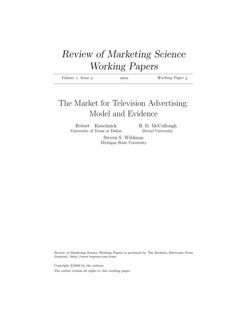
3.4 Parametric Estimates of the Relationship
Turning to an examination of the evidence on whether the national television
advertising market is segmented, we note that equation (10) above suggests that COST
should be linear in BO and C where BO represents the number of broadcast-only viewers
and C the number of �cable�viewers. Our evidence that COST is linear in TOT is
consistent with this presumption, since TOT=BO+C. An examination
of Figure 2 further supports this inference as COST appears linear in BO, given C, and
COST appears to be linearly related to BO and C.10
To test this hypothesis, we regress COST on BO, BO2, C, BO×C and C2, and
compare its results to a regression of COST on BO and C. The resulting Wald test
statistic equals1.958 and thus fails to reject the joint hypothesis that 2BOβ , BO Cβ × and
2Cβ equal zero. Trivariate coplots (Cleveland, 1993) also indicate that COST is linear in
both BO conditional on C and C conditional on BO. Consequently, we reject the
hypothesis that COST is nonlinear in BO and C.
If the �law of one price� holds, then the price of an additional broadcast-only
10 We omit lines of best fit in Figure 2 because it is inappropriate to impute all of COST to either BO or C.
19Kieschnick et al.: The Market for Television Advertising
Produced by The Berkeley Electronic Press, 2011
viewer should be equal to the price of an additional cable viewer. To test this proposition,
we estimate the following regression:
0
2
0.33 0.0049 0.0242( 0.03) (0.50) (9.26)0.7755
BO CCOST BO CBO C
R
β β β ε= + + +− + +−
=
(13)
with t-statistics reported in parentheses. These results are inconsistent with the law of one
price: the point estimates imply two and one-half cents per cable viewer, and one-half of
one cent per broadcast viewer. However, the insignificance of BOβ implies that
advertisers are not paying for broadcast-only viewers. Since the proportion of broadcast-
only viewers ranges from 0.15 to 0.40, we find this difficult to accept. The high R2 and
insignificant t-statistics suggest collinearity as a reason for this aberrant result. The
standard diagnostics (Judge, et al, 1988, §21.3.1) indicate the presence of
multicollinearity. The simple correlation between BO and C is 0.85, which is high, and is
greater than the R2 from Eq. 13. Rescaling the independent variables to have unit length,
but not recentering, yields a largest-to-smallest eigenvalue ratio whose square root is
11,938. These results suggest that further analysis of multicollinearity is warranted.
3.5 Diagnosing Multicollinearity
Multicollinearity does not mean that all coefficients will be estimated with great
imprecision. In fact, it is possible to determine which coefficients will be estimated
precisely and which coefficients will be estimated imprecisely due to the
multicollinearity. However, further analysis is necessary to accomplish this.
The possible effect of this multicollinearity can be assessed in the usual fashion
using Silvey's (1969) method (see also Judge, et al, 1985, §22.3) and Belsley's (1991)
guide to implementing the method. For this analysis the variables are rescaled to have
unit length but are not recentered (Belsley, 1991, §3.3).
First note that the variance of an individual coefficient can be written as,
2 2
1var( )
K
k kj jj
b pσ λ=
= ∑ , (14)
20 Review of Marketing Science Working Papers Vol. 1 [2002], No. 2, Working Paper #5
http://www.bepress.com/roms/vol1/iss2/paper5
where 2σ is the error variance and jkp is the k-th element of the normalized eigenvector
associated with the j-th eigenvalue, jλ . The proportion of var( )kb associated with any
single characteristic root is
2
2
1
kj jkj K
kj jj
p
p
λφ
λ=
=∑
(15)
and the condition indices of X are given by maxj jη λ λ= so that jλ necessarily assumes its
minimum of 1.0 for some j.
Table 3 gives the variance-decomposition proportions, where the leftmost column
gives the condition index and each of the three rightmost columns sums to unity. The
condition indices are extremely large, since a condition index in excess of 30 is
considered evidence of multicollinearity. Examining the condition indices, we see
immediately that the third eigenvalue is troublesome, and the second eigenvalue might
be. The presence of two or more large kjφ in a row indicates that multicollinearity
associated with that row's characteristic root adversely affects the precision of the
estimated coefficients. Here, kjφ > 0.50 is taken to be large (Belsley, et al, 1980). Hence,
we conclude that the third eigenvalue alone is the source of the multicollinearity.
The multicollinearity induced by the third eigenvalue does not necessarily affect
all the coefficients, since from Eq. 14 we see that the k-th coefficient is unaffected by the
j-the root as long as kjp is small. Table 4 gives the matrix of normalized eigenvectors.
Examining the third row, we see that 3,3p is small, so we can expect a good estimate of
Cβ . From the second row, 2,3p is not small, so we can expect that the estimate of
BOβ will be substantially affected by the multicollinearity, and will be "nearly
inestimable''. Vinod and Ullah (1981, §5.3.2) explain how near inestimability arising
from multicollinearity can lead to "wrong'' signs or insignificance, casting further doubt
on the validity of (13). Based on a priori knowledge of the broadcast industry and
the eigenvalue analysis, we believe that accurate parameter estimates will show that Cβ is
"close'' to two and one half cents and that BOβ is not "close'' to one half of one cent.
21Kieschnick et al.: The Market for Television Advertising
Produced by The Berkeley Electronic Press, 2011

3.6 'Solving' the multicollinearity problem
Any particular multicollinearity problem can be characterized either as a sample
problem or a population problem. In the former case, the best solution is to increase the
sample size. In the present case, television programs with a larger broadcast-only
audience tend also to have a larger cable audience, so the problem can be characterized as
a population problem. The textbook remedies (drop a variable, principal component
regression, etc.) are all unsatisfactory. To estimate the change in cost attributable to a
marginal change in the number of broadcast-only viewers, BOβ , ideally we should like to
regress that part of cost not attributable to non-broadcast viewers, (C - Cβ C), on the
number of broadcast only viewers, BO; i.e., regress (C - Cβ C) on BO. Unfortunately,
this method for estimating BOβ assumes that we already know Cβ . Similarly, if we
already knew BOβ , then we could regress (C - BOβ BO) on C to estimate the change in
cost due to a marginal increase in the number of cable viewers, Cβ . Obviously, we
cannot directly pursue either of these strategies because we do not have a priori
knowledge of either Cβ or BOβ . However, we can pursue equivalent strategies that will
lead to good estimates of Cβ and BOβ that are not contaminated by multicollinearity.
To obtain accurate estimates of BOβ and Cβ , we shall reduce the dimension of
the parameter space (Judge, et al, 1984, §22.4.2), and then reparametrize the model
(Spanos, 1986, §20.5 gives the theory; Hendry, 1996, p. 276 gives an example).
Moreover, the transformed model provides for direct estimation of the parameters of
interest, so there is no need to "reinterpret'' our estimates in term of the original
parameters.
For each program the marginal cost of an "average'' viewer must be the weighted
sum of the costs of broadcast and cable viewers. We take this to be the linear weighted
sum:
T BO BO C Cβ γ β γ β ε= + + (16)
where BOγ is the proportion of the audience which is broadcast-only and Cγ is the
proportion of the audience which is cable. Since this holds true for individual
22 Review of Marketing Science Working Papers Vol. 1 [2002], No. 2, Working Paper #5
http://www.bepress.com/roms/vol1/iss2/paper5
observations, it must hold true for the means, which we shall denote with an overbar.
Define the two series ( )BO BO BO Cγ = + and ( )C C BO Cγ = + which have means BOγ =
0.2991 and NBγ =0.7009, respectively, and a common standard error of the sample mean,
0.0046.
Solving (16) for BOβ , using BOγ , Cγ and �Tβ for BOγ , Cγ , and Tβ , substituting
into (13), and rearranging yields the following reparametrized regression
3
2
13.1 0.0230( 4.7) (9.52)0.4858
T CC
BO BO
COST BO c C
R
β γβ εγ γ
− = + − +
−−
=
(17)
which has one less dimension than the multicollinear regression (13). Note that this
estimate of Cβ =0.0230 is "close'' to two and one-half cents.
Repeating the procedure, this time focusing on BOβ yields �BOβ = 0.0145 with a t-
stat of 2.604. Note that this estimate of Cβ = 0.0145 is not "close'' to one-half of one
cent, but is instead almost one and one-half cents. The reparameterization (17) might
appear ungainly, though it has a simple intuition. Some algebra (see the Appendix) shows
that the regression (17) is equivalent to:
3BO CCOST BO c Cβ β ε− = + + (18)
The left hand side of this equation is simply COST less that portion attributable to
broadcast viewers.11 Thus the reparameterization (17) is equivalent to a regression on the
portion of COST attributable to cable viewers on the number of cable viewers. A similar
interpretation holds for the reparameterization effected by focusing on BOβ .
Of interest is whether the fit based on the reparameterized results is significantly
different than the initial least squares result. Regressing COST on the artificial variable
W= 0.0145 BO + 0.0230 C yields:
11 Because there is a constant term on the right hand side and only the slope is of interest, it is immaterial whether we specify the COST attributable to broadcast viewers at α+βBOBO or just βBOBO.
23Kieschnick et al.: The Market for Television Advertising
Produced by The Berkeley Electronic Press, 2011
4
2
7.6 0.9595( 1.0) (18.10)0.7734
WCOST c WW
R
β ε= + +−−
=
(19)
whose R2 compares favorably with the results of Equation 4. A test for loss of fit
(Greene, 1997, §7.4), treating (19) as the restricted regression, yields F(1,95)=0.87 with
m.s.l. = 0.352. Thus the fits of Equations 13 and 19 are in substantial agreement.
We see, then, that an advertiser will pay about 2.3 cents for an additional cable
viewer, and just under 1.5 cents for an additional broadcast viewer,
i.e., an additional cable viewer is 59% ( = 100(0.0230/0.0145 - 1)%) more valuable to the
network than an additional broadcast viewer. The difference in prices paid is consistent
with our model of the market for television advertising, and strongly rejects the �law of
one price� for television advertising.
4. Summary and Conclusions
While advertising plays a critical role in the funding of media, including Internet,
in the United States, economists have devoted little attention to the pricing of advertising.
This paper presents a model of a competitive market for television advertising time for
which it is shown that per viewer prices may vary among programs, and, for broadcast
programs, that different implicit per-viewer prices may be charged for those members of
their audiences that do and do not subscribe to cable or satellite services. These
predictions stand in stark contrast to the nearly standard assumption, going back to
Steiner (1952) that a common per viewer price must apply to all ad units sold in these
same markets.
Our econometric study of broadcast network advertising prices for 108 prime time
programs suggests that networks are effectively charging substantially different per
viewer prices for the cable viewers (non-broadcast only viewers) in their audiences than
for their broadcast-only viewers. This evidence supports the model proposed in this
paper and rejects the standard assumption that prices in advertising markets are subject to
the �law of one price� regardless of mode of delivery. Interestingly, our results are
24 Review of Marketing Science Working Papers Vol. 1 [2002], No. 2, Working Paper #5
http://www.bepress.com/roms/vol1/iss2/paper5
consistent with Liebowitz�s (1982) evidence that cable segmented the television
advertising market in Canada.
As a parting comment, we note that technologies marrying the Internet and
television are making it possible for advertisers to better track the viewers of programs
they advertise on. The recent controversy over Tivo�s use of its Internet connection to
upload data on its subscribers� viewing habits is one example of what is now possible and
will become more prevalent in the future. This feature of an Internet TV service can be
incorporated in the model developed above by eliminating the likelihoods associated with
viewers� choices. Instead the expressions for the value of advertising time will have only
the r component of the expressions for the probability of the advertiser�s commercial
being noticed on a particular program, and only programs actually watched (rather than
the larger set of potentially watched programs) will be retained in these expressions.
With interactive commercials, advertisers would also have firmer knowledge of whether
their commercials were noticed as well, which would modify r. Consequently we expect
the considerations put forth in this paper to be applicable to future video advertising as
technology changes the delivery of video programming.
25Kieschnick et al.: The Market for Television Advertising
Produced by The Berkeley Electronic Press, 2011
References Belsley, D. A. (1991), "A Guide to Using the Collinearity Diagnostics,'' Computer Science in Economics and Management, 4, 33-50 Belsley, D. A. (1991), Conditioning Diagnostics: Collinearity and Weak Data in Regression, New York: Wiley Belsley, D. A., E. Kuh and R. E. Welsh (1980), Regression Diagnostics: Identifying Influential Data and Sources of Collinearity, New York: Wiley Blair, R. D. and Romano, R. E. (1993), �Pricing Decisions of a Newspaper Monopolist,� Southern Economics Journal, 59(4), 721-732. Chaudhri, V. (1998), �Pricing and Efficiency of a Circulation Industry: The Case of Newspapers,� Information, Economics and Policy, 10(1), 59-76. Dixit, A. K. and Stiglitz, J. E. (1977), �Monopolistic Competition and Optimum Product Diversity,� American Economic Review, 67, 297-308. Cleveland, W. S. (1993), Visualizing Data, Summit, NJ: Hobart Press Federal Communications Commission, 1980, The Market for Television Advertising, Network Inquiry Special Staff Report. Fournier, G., and D. Martin (1983), "Does Government-Restricted Entry Produce Market Power?: New Evidence from the Market for Television Advertising,'' Bell Journal of Economics, 14, 44-56 Goettler, R., and R. Shachar (1996), "Estimating Show Characteristics and Spatial Competition in the Network Television Industry'', Yale Working Paper Series H, \# 5. Hawkins, D. M. (1980), Identification of Outliers, New York: Chapman and Hall Judge, G. C., R. C. Hill, W. E. Griffiths, H. Lütkepohl, and T. C. Lee (1985), The Theory and Practice of Econometrics, New York: Wiley Judge, G. C., R. C. Hill, W. E. Griffiths, H. Lütkepohl, and T. C. Lee (1988), Introduction to the Theory and Practice of Econometrics, New York: Wiley Liebowitz, S.J., 1982, �The impacts of cable retransmission on television broadcasters,� Canadian Journal of Economics 3, 503-524
26 Review of Marketing Science Working Papers Vol. 1 [2002], No. 2, Working Paper #5
http://www.bepress.com/roms/vol1/iss2/paper5
Lilien, G., P. Kotler, and K. Moorthy (1992), Marketing Models, Englewood Cliffs: Prentice-Hall, Inc. Moulton, B. R. (1991), "A Bayesian approach to regression selection and estimation, with application to a price index for radio services,'' Journal of Econometrics, 49, 169-193. Nielsen Media Research (1996a), National Audience Demographics Volume 2: November 1996. Nielsen Media Research (1996b), Households and Cost Per Thousand: November 1996. Owen, B., J. Beebe, and W. Manning (1974), Television Economics, Lexington, MA: D.C. Heath & Co. Owen, B. and S. Wildman (1992), Video Economics, Cambridge, MA: Harvard University Press. Silvey, S. D. (1969), "Multicollinearity and Imprecise Estimation,'' Journal of the Royal Statistical Society, Series B, 35, 67-75. Spence, A. M. (1976), �Product Selection, Fixed Costs, and Monopolist Competition,� Review of Economic Studies, 43, 217-235. Steiner, P.O. (1952), �Program Patterns and Preferences, and the Workability of Competition in Radio Broadcasting,� Quarterly Journal of Economics 66, 194-223. Vinod, H. D. and A. Ullah (1981), Recent Advances in Regression Methods, New York: Marcel Dekker. Wildman, S. and D. Cameron (1989), "Competition, Regulation, and Sources of Market Power in the Radio Industry,'' Working Paper. Wildman, S. and Owen, B. (1985), �Program Competition, Diversity and Multichannel Bundling in the New Video Industry,� in E. Noam, ed., Video Media Competition: Regulation, Economics, and Technology, New York: Columbia University Press. Wildman, S. (1998), "Toward a Better Integration of Media Economics and Media Competition Policy,'' in A Communications Corunucopia: Markle Foundation Essays on Information Policy, edited by Roger G. Noll and Monroe E. Price, Washington, D. C.: Brooking Institution Press.
27Kieschnick et al.: The Market for Television Advertising
Produced by The Berkeley Electronic Press, 2011
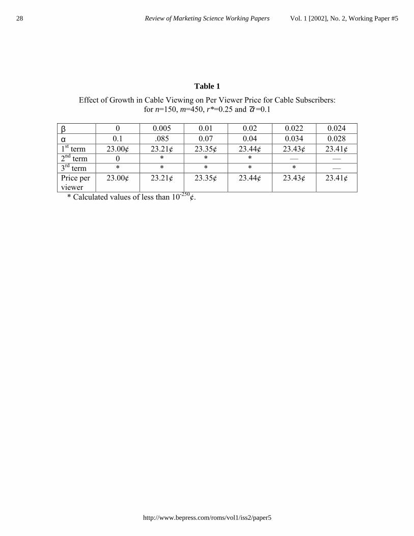
Table 1
Effect of Growth in Cable Viewing on Per Viewer Price for Cable Subscribers: for n=150, m=450, r*=0.25 and α =0.1
β 0 0.005 0.01 0.02 0.022 0.024 α 0.1 .085 0.07 0.04 0.034 0.028 1st term 23.00¢ 23.21¢ 23.35¢ 23.44¢ 23.43¢ 23.41¢ 2nd term 0 * * * � � 3rd term * * * * * � Price per viewer
23.00¢ 23.21¢ 23.35¢ 23.44¢ 23.43¢ 23.41¢
* Calculated values of less than 10-250¢.
28 Review of Marketing Science Working Papers Vol. 1 [2002], No. 2, Working Paper #5
http://www.bepress.com/roms/vol1/iss2/paper5

Table 2
Effect of Growth in Cable Viewing on Per Viewer Price for Cable Subscribers: for n=20, m=50, r*=0.25 and α =0.5
β 0 0.05 0.08 0.10 0.12 0.14 α 0.5 0.375 0.3 0.25 0.20 0.15 1st term 14.41¢ 16.61¢ 17.33¢ 17.55¢ 17.53¢ 17.30¢ 2nd term 0 ** ** ** ** ** 3rd term ** ** ** ** ** ** Price per viewer
14.41¢ 16.61¢ 17.33¢ 17.55¢ 17.53¢ 17.30¢
** Calculated values of less than 10-10¢.
29Kieschnick et al.: The Market for Television Advertising
Produced by The Berkeley Electronic Press, 2011
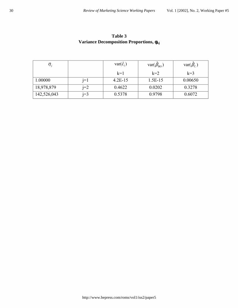
Table 3
Variance Decomposition Proportions, φφφφkj
jη 1�var( )c �var( )BOβ �var( )Cβ
k=1 k=2 k=3 1.00000 j=1 4.2E-15 1.5E-15 0.00650 18,978,879 j=2 0.4622 0.0202 0.3278 142,526,043 j=3 0.5378 0.9798 0.6072
30 Review of Marketing Science Working Papers Vol. 1 [2002], No. 2, Working Paper #5
http://www.bepress.com/roms/vol1/iss2/paper5
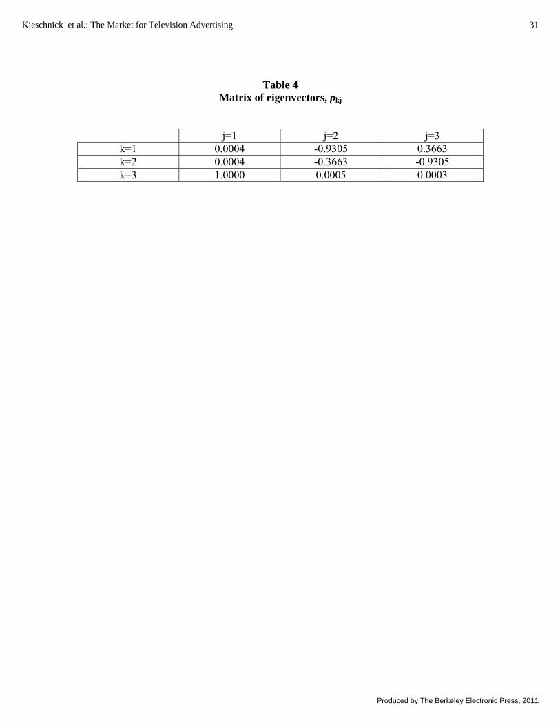
Table 4
Matrix of eigenvectors, pkj
j=1 j=2 j=3 k=1 0.0004 -0.9305 0.3663 k=2 0.0004 -0.3663 -0.9305 k=3 1.0000 0.0005 0.0003
31Kieschnick et al.: The Market for Television Advertising
Produced by The Berkeley Electronic Press, 2011
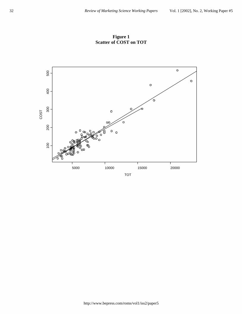
Figure 1
Scatter of COST on TOT
TOT
CO
ST
5000 10000 15000 20000
100
200
300
400
500
32 Review of Marketing Science Working Papers Vol. 1 [2002], No. 2, Working Paper #5
http://www.bepress.com/roms/vol1/iss2/paper5

Figure 2
Scatter of COST on BO(x) and C(+)
Number of Viewers (000)
CO
ST
2000 4000 6000 8000 10000 12000
5010
015
020
025
030
0
33Kieschnick et al.: The Market for Television Advertising
Produced by The Berkeley Electronic Press, 2011

Appendix
Ideally, letting C=COST, we would like to estimate 3BO CC BO c Cβ β ε− = + +
We show that the above is algebraically equivalent to (18), which we repeat immediately below:
3CT
CBO BO
C BO c C BOγβ β εγ γ
− = + − +
(18a)
What can be made of the slope term?
C CC C C
BO BO
C BO C BOγ γβ β βγ γ
− = −
Look now at the second term on the RHS. Solving (17) for Cβ and inserting,
C T BO BO CC
BO C BO
T BO BO
BO
TBO
BO
BO BO
BO
BO BO
γ β γ β γβγ γ γ
β γ βγ
β βγ
−− = − −= −
= − +
So we can rewrite (18) as: 3CT
C BOBO BO
C BO c C BO BOγβ β β εγ γ
− = + − + + .
Adding T
BO
BOβγ
to each side yields: 3 C BOC c C BOβ β ε= + + + .
Subtracting BO BOβ from each side yields: 3BO CC BO c Cβ β ε− = + +
Q.E.D.
34 Review of Marketing Science Working Papers Vol. 1 [2002], No. 2, Working Paper #5
http://www.bepress.com/roms/vol1/iss2/paper5
Recommended